M.M. Ahmed and S.S. Ahmed Mining and Metallurgical ... of Engineering Sciences, Assiut University, Vol. 36, No. 1, pp. 147- 166, January 2008 147 A COMPARISON STUDY TO DETERMINE THE

Journal of Engineering Sciences, Assiut University, Vol. 36, No. 1, pp. 147- 166, January 2008

147

A COMPARISON STUDY TO DETERMINE THE MEAN OF PARTICLE SIZE DISTRIBUTION FOR TRUTHFUL

CHARACTERIZATION OF ENVIRONMENTAL DATA (PART 1)

M.M. Ahmed and S.S. Ahmed Mining and Metallurgical Engineering Department, Faculty of

Engineering, Assiut University, Assiut 71516, Egypt

Email: [email protected]

(Recieved December 3, 2007 Accepted January 8, 2008)

One of the most important steps in environmental studies is to get an

accurate distribution of the pollutants in terms of its quantity and

qualities. Some environmental studies are acquiring a good

classification of the particle size including the average mean of the

particle. Many researchers use the median size (x50) or until the size

passing 80% cumulative undersize (x80) as a measure for evaluation of

the particle size distribution resulted from different mineral processing

operations such as crushing, grinding, classification, sedimentation,

and/or solid-liquid separation or even during the study of the pollutant

settlement. These measures are not so accurate to differentiate between

different particle size distributions (PSDs) because many PSDs data sets

may have the same values of x50 or x80 if these data sets are represented

between the particle size, x and the cumulative undersize distribution, F

(x). This paper is a trial to introduce a new methodology to determine the

mean of a particle size distribution (MPSD) accurately using Gates-

Gaudin-Schuhmann and Rosin-Rammler models. The value of this

measure takes into consideration all particle sizes and their

corresponding distributions. The results showed that the different PSD,

which have the same values of median (x50) have different values of this

measure, especially with Rosin-Rammler model. In this paper, the

expressions of different types of means of a particle size distribution

(arithmetic, quadratic, cubic, geometric, and harmonic) were derived

mathematically using the two mentioned models. It is recommended to

select RR model to be applied in estimation of the different means of a

particle size distribution because it fits the available data better than the

GGS model, as well as, it determines the correct values and exerts the

actual differences between the different means of different particle size

distribution data sets. This work will be continuing by demonstrating a

case study using real environmental data in Part (2).

KEY WORDS: Frequency or density function, distribution function,

particle size, mean, Gates-Gaudin-Schuhmann model, Rosin-Rammler

model

M.M. Ahmed and S.S. Ahmed 148

NOMENCLATURE

c the particle size corresponding to 63.2% cumulative distribution undersize

f (x) particle size distribution frequency function either by number,

length, surface, or mass, whichever may be of interest

fL (x) particle size distribution by length

fM (x) particle size distribution by mass

fN (x) particle size distribution by number

fS (x) particle size distribution by surface

GGS Gates-Gaudin-Schuhmann

k the maximum size of particles which corresponding to 100%

cumulative distribution undersize

k1, k2, k3 shape factors

m a characteristic constant of the material under analysis and gives

a measure of steepness of cumulative curve

m (x) a certain function of particle size x

)x( m-

the area under the distribution curve with respect to F (x) axis

MPSD mean of particle size distribution

n a characteristic constant of the material under analysis and gives

a measure of steepness of cumulative distribution curve

PSD particle size distribution

R2 coefficient of correlation

RR Rosin-Rammler

x particle size

x50 the median or the size which corresponds to 50% cumulative undersize

x80 the size which corresponds to 80% cumulative undersize

)x(-

mean diameter

a

-

)x( arithmetic (length) mean

c

-

)x( cubic (volume) mean

g

-

)x( geometric mean

h

-

)x( harmonic (surface volume) mean

q

-

)x( quadratic (surface) mean

y = F (x) cumulative undersize distribution function

INTRODUCTION

Primary properties of particles such as the particle size distribution, shape, density, and

surface properties govern the secondary properties such as the settling velocities of

particles, the permeability of a bed, or the specific resistance of a filter cake.

Knowledge of these properties is a vital in the design and operation of mineral

processing equipment [1].

A Comparison Study to Determine the Mean of Particle……. 149

Particle size is probably the most important single physical characteristic of

solids. It influences the combustion efficiency of pulverized coal, the settling time of

cements, the flow characteristics of granular materials, the compacting and sintering

behavior of metallurgical powders, pharmaceutical products, and the masking power of

paint pigment [2]. These examples illustrate the intimate involvement of particle size in

energy generation, industrial processes, resource utilization, and many other

phenomena [3].

Crushing and grinding operations are employed to fracture mineral aggregates,

and thus to increase liberation. The choice of fineness of grinding is an important

decision as the ore must be sufficiently finely ground to liberate the valuable minerals.

The accurate determination of grain liberation during reduction has a significant impact

on the advancing of physical or chemical mineral processing operations. Deriving a

measure that can be used to estimate quantitatively the fineness of grinding becomes of

great practical utility [4].

The maximum utilization of particle size distribution data can be obtained if

the data was represented by a mathematical expression. The mathematical function

allows ready graphical representation and offers maximum opportunities for

interpretation, extrapolation, and comparison of different PSDs [5]. Furthermore, more

useful information can be revealed if the parameters of the function can be related to

the properties of the particulate system or process that produces it. This would allow of

product control, tighter product specifications and quality assurance [1].

Several parameter mathematical models and expressions have been developed

to obtain the distribution and density functions from experimental PSD curves. These

functions range from the well-established normal and log-normal distributions to the

RR and GGS models [1,3,5]. The RR distribution function has long been used to

describe the PSD of powders of various types and sizes. This function is particularly

suited to represent powders made by grinding, milling, and crushing operations [3].

Numerous three and four parameter models have also been proposed for greater

accuracy in describing particle size distributions. But they have limit applications due

to their greater mathematical complexity [1].

AIM OF THE WORK

Many researchers [5-9] have used the median (x50) or x80 to compare and evaluate

different particle size distributions. But, these measures may be not so accurate and

enough to differentiate between different distributions because different particle size

distributions may have the same values of x50 or x80. The aim of this research is to

compare the mean of a particle size distribution (MPSD) estimated from Gates-

Gaudin-Schuhmann and Rosin-Rammler models for different particle size distribution

data sets. The value of this index is a valuable and more reliable to be used to

differentiate between different PSDs which have the same values of x50. Also, it was

derived expressions which can be used to determine mathematically the values of

different types of means of a distribution (arithmetic, quadratic, cubic, geometric, and

harmonic) using the two mentioned models. This paper may be the first one developed

to derive the mean of a particle size distribution from Gates-Gaudin-Schuhmann and

Rosin-Rammler models.


TYPES OF PARTICLE SIZE ANALYSIS

An irregular particle can be measured by a number of different sizes which depend on

the dimension and/or property studied. There are basically three groups of sizes,

namely, equivalent sphere diameter, equivalent circle diameter, and statistical diameter

[10]. The first type of sizes is defined as the diameter of a sphere which would have the

same property as the particle itself (the same volume, the same projected area, the same

settling velocity, etc.). The second type of sizes is defined as the diameter of a circle

that would have the same property as the projected outline of the particle. The

statistical diameter is obtained when a linear dimension parallel to a fixed direction is

measured [1,5].

Many methods have been developed to determine the size distribution of

particulate system [11-12]. A number of methods aimed at determining PSDs (i.e.,

sieving, cycloning, microscopy, etc.) have been described [13]. Using different

characterization techniques for the PSD analysis of a material, one may obtain quite

radically different information and different measures of size [14-15]. Hence, any

analysis technique used will depend on the ultimate goal of the characterization [3].

In methods of solid-liquid separation at which the motion of a particle relative

to the fluid is the governing mechanism, it is of course most relevant to use a method

which measures the free-falling diameter or, more often, the Stokes’ diameter [5,10]. In

liquid filtration on the other hand, the surface volume diameter is more relevant to the

mechanism of separation because the resistance to flow through packed beds depends

on the specific surfaces of the particles that make up the bed [1].

TYPES OF PARTICLE SIZE DISTRIBUTIONS (PSDS)

Four different types of a particle size distribution may be defined, as follows:

1. Particle size distribution by number, fN (x).

2. Particle size distribution by length, fL (x).

3. Particle size distribution by surface, fS (x).

4. Particle size distribution by mass, fM (x).

Although that the above distributions are related together, the conversion from

one distribution to another is possible only when the shape factor is constant, i.e.

particle shape is independent on particle size. The following relationships show the

basis of such conversion [1]:

(x)N

x f k (x) L

f1

(1)

(x)N

f x k (x) S

f2

2 (2)

(x)N

f x k (x) M

f3

3 (3)

The constants k1, k2, and k3 contain the shape factor which depends often on

particle size distribution. This assures that the accurate conversion from one type of

particle size distribution to another is not possible without a full quantitative

knowledge of the shape factor’s dependence on particle size. These constants can easily

be found if the shape of particles does not vary with size.


From the definition of frequency distribution, the area under the frequency

curve against particle size should be equal to one. This can be revealed by the

following equation [16-17]:

01

0

. dx f (x)

(4)

where: f (x) = particle size distribution frequency function either by number, length,

surface, or mass, whichever may be of interest

Different methods give different particle size distributions and the selection of

the method is made on the basis of particle size and the type of distribution required. In

most applications, particle size distribution by mass is of interest. There are, however,

cases such as liquid clarification where the turbidity of the overflow is of importance

and particle size distribution by surface or even by number are more relevant [1].

Representation of the Particle Size Distribution Data

Particle size distribution data are given either in an analytical form (as a function) or as

a set of data in a table or a diagram. The distributions are represented as frequencies, f

(x) or cumulative frequencies, F (x) which mutually corresponds because the frequency

curve can be obtained by differentiation of the cumulative curve as follows [16,18]:

dx

dF (x) f (x) (5)

or vice versa, the cumulative curve, F (x) can be obtained by integration of the

frequency curve, f (x), i.e.:

f (x) dx F (x) (6)

where: F (x) = cumulative undersize distribution function.

The area under the frequency curve is, by definition, equal to 1.0 as given in

equation (4), so that F (x) goes from 0 to 1.0 or 100%. The cumulative percentages are

given as either oversize or undersize, which mutually correspond, because the sum of

oversize and undersize fractions are equal to one at any given particle size [1,16].

The Measures of a Particle Size Distribution

There are great number of different average or mean sizes which may be defined for a

given particle size distribution. The purpose of such measures is to represent a

population of particles by a single figure. There are three important measures for a

given particle size distribution. These are the mode, the median, and the mean

[9,16,19].

a. The mode

The mode is defined as the most commonly occurring size or the size corresponding to

the peak on the size distribution frequency curve. This measure is not a valid for

comparisons of different distributions because some distributions may have more than

one peak and are commonly referred to as multi-modal distributions [1,16].


b. The median

The median or the 50% size (x50) is the size at which half of the particles are larger and

the other half are smaller. The median is most easily determined from the cumulative

undersize or oversize curves, i.e. it is the size which corresponds to 50%. This

measure may be not also so accurate and valuable measure to differentiate between

different particle size distributions (PSDs) data because different particle size

distribution data sets may have the same values of median [1,5,20].

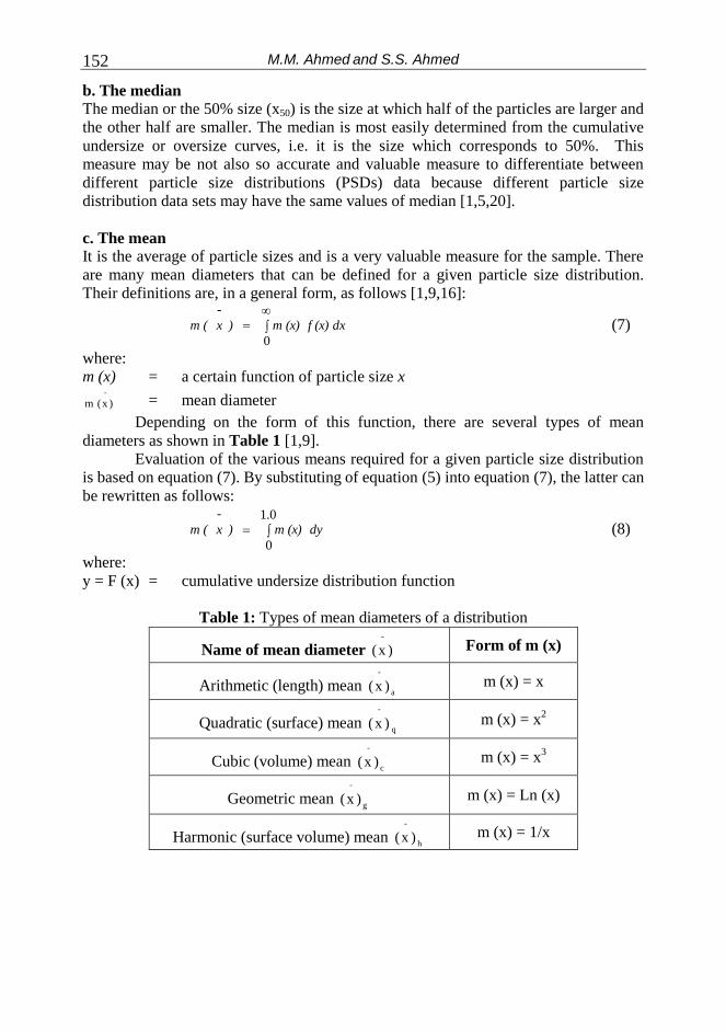
c. The mean

It is the average of particle sizes and is a very valuable measure for the sample. There

are many mean diameters that can be defined for a given particle size distribution.

Their definitions are, in a general form, as follows [1,9,16]:

f (x) dxm (x) )

-

xm (

0

(7)

where:

m (x) = a certain function of particle size x

)x( m-

= mean diameter

Depending on the form of this function, there are several types of mean

diameters as shown in Table 1 [1,9].

Evaluation of the various means required for a given particle size distribution

is based on equation (7). By substituting of equation (5) into equation (7), the latter can

be rewritten as follows:

dy.

m (x) )

-

xm ( 01

0

(8)

where:

y = F (x) = cumulative undersize distribution function

Table 1: Types of mean diameters of a distribution

Name of mean diameter )x(-

Form of m (x)

Arithmetic (length) mean a

-

)x( m (x) = x

Quadratic (surface) mean q

-

)x( m (x) = x

2

Cubic (volume) mean c

-

)x( m (x) = x

3

Geometric mean g

-

)x( m (x) = Ln (x)

Harmonic (surface volume) mean h

-

)x( m (x) = 1/x


m (x)

F (

x)

Fig. 1: Evaluation of a mean )x( -

of a particle size distribution from the cumulative

undersize distribution function (F (x))

If either frequency function, f (x), or cumulative undersize distribution

function, F (x) is available as analytical functions, the desired mean is evaluated by

integration of equations (7) or (8), respectively. If, however, no analytical function is

fitted and the particle size distribution is in the form of a graph or a table, evaluation of

mean diameters can be best done graphically. If the cumulative undersize function, F

(x) was plotted against m (x) for the corresponding type of size required, the mean size,

)x( m-

is then represented by the area under the curve with respect to F (x) axis as

illustrated in Figure 1 [1]. The mean size is evaluated from this area using the

corresponding equation for m (x) as shown in Table 1.

Determination of the Mean of Particle Size Distribution (MPSD) Using Gates-Gaudin-Schuhmann Distribution Model:

Referring to the availability of many progressive computer softwares, it is more

convenient to fit the experimental particle size distribution data with an analytical

function and to use this function mathematically in further treatment. It can be decided

that it is easier to evaluate the mean size from analytical functions more than from

experimental data. The Gates-Gaudin-Schuhmann distribution function is a widely

used function which is usually applied to evaluate the particle size distribution data

resulted from comminution processes [3,5,18,21-25]. It is a two parameter distribution

function which can be expressed by the following function: n

k

x F (x) y

(9)

where:


x = particle size

k = the maximum size of particles which corresponding to 100%

cumulative distribution undersize

Area = )x( m-


n = a characteristic constant of the material under analysis and

gives a measure of steepness of cumulative distribution curve

Equation (9) may be rewritten as follows:

n k yx

1

(10)

The frequency distribution function can be obtained by differentiation of equation (9)

as follows:

1n- x

nk

n

dx

dF (x)

dx

dy f(x) (11)

Equation (9) can be reduced to the following formula:

- n Ln (k) n Ln (x) Ln (y) (12)

Equation (12) gives a straight line if Ln (y) is plotted against Ln (x) where n is

the slope of the best fitting line of the data and - n Ln (k) is the intercept part of the Ln

(y) axis. Both the constants n and k can be obtained easily using the least squares

method through computer software.

The various mean sizes available in Table 1 may be easily determined from

Gates-Gaudin-Schuhmann distribution function as explained below. For example, if it

is required to obtain the arithmetic mean size, this may be evaluated by integration of

equations (7) or (8) after replacing m (x) by x. In this case, the equations may be

rewritten as follows:

f (x) dxx ) a)

-

xm ((

0

(13)

or:

dy.

x ) a)

-

xm (( 01

0

(14)

From integration rules, it is better and easier to use equation (14). Replace the

value of x in equation (10) by y and then substitute in equation (14), this change the

latter one into the following form:

dy.

ny k) a)

-

xm (( 01

0

1

(15)

By integration of the previous equation and substitution the values of

integration limits of y by (0, 1.0), the final expression of arithmetic mean may be

determined as follows:

1 n

n k ) a)

-

x m (( a)

-

x(

(16)

To determine the values of other mean sizes, the value of m (x) in equation (8)

is substituted by x2 (quadratic mean), x

3 (cubic mean), Ln (x) (geometric mean), and 1/x

(harmonic mean). Hence, by applying the same previous procedure, the final

expressions of different mean sizes may be obtained as follows:

2 n

n k )

q)

-

xm (( q)

-

x(

(17)


3

3

3

n

n k )

c)

-

xm (( c)

-

x(

(18)

n

n Ln (k) -

e

)g

)

-

xm ((

e g)

-

x(

1

(19)

n

) k(n -

)h

)

-

xm ((

h

)

-

x(11

(20)

Although the mean particle size of the distribution (MPSD) is more convenient

and valuable than the other measures, because it takes into consideration the complete

distribution of the sizes and their corresponding percentages, this measure has some

drawbacks with Gates-Gaudin-Schuhmann distribution model. Firstly, it is possible to

obtain the same value of this measure with different distributions. This may be

occurred if the distributions have corresponding values of the model constants, n and k.

Also, this measure may have a negative value of the harmonic mean if the value of the

steepness of cumulative distribution curve of the data, n is lesser than the unity.

Determination of the Mean of Particle Size Distribution (MPSD) Using Rosin-Rammler Distribution Model:

The Rosin-Rammler distribution function is a commonly used model which is usually

applied to evaluate the particle size distribution data. The Rosin-Rammler function is

particularly suited for representing particles generated by grinding, milling and

crushing operations. This model has long been used by many researchers [2,3,5,22,26]

to describe the particle size distribution of powders of various types and sizes. It is a

two parameter distribution model and can be expressed by the following general

equation:

m

c

x- - F (x) y exp1 (21)

where:


x = particle size

c = the particle size corresponding to 63.2% cumulative distribution

undersize

m = a characteristic constant of the material under analysis and gives a

measure of steepness of cumulative curve

Equation (21) may be rewritten as follows:

/m)( y)] Ln ( c [x

11 (22)

The frequency distribution function can be obtained by differentiation of

equation (21) as follows:


m

m -

mc

x- x

c

m

dx

dF (x)

dx

dy f(x) exp

1 (23)

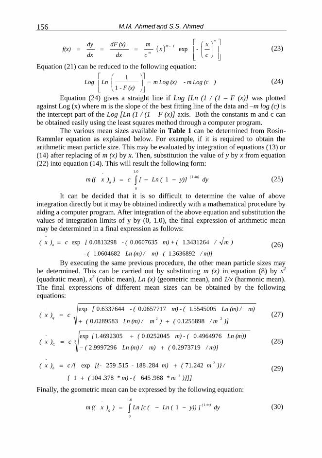
Equation (21) can be reduced to the following equation:

)- m Log (cm Log (x) - F (x)

Ln Log

1

1 (24)

Equation (24) gives a straight line if Log [Ln (1 / (1 – F (x)] was plotted

against Log (x) where m is the slope of the best fitting line of the data and –m log (c) is

the intercept part of the Log [Ln (1 / (1 – F (x)] axis. Both the constants m and c can

be obtained easily using the least squares method through a computer program.

The various mean sizes available in Table 1 can be determined from Rosin-

Rammler equation as explained below. For example, if it is required to obtain the

arithmetic mean particle size. This may be evaluated by integration of equations (13) or

(14) after replacing of m (x) by x. Then, substitution the value of y by x from equation

(22) into equation (14). This will result the following form:

dy y)] Ln ([ c ) )x m ((

.

/m)(

a

-

01

0

11 (25)

It can be decided that it is so difficult to determine the value of above

integration directly but it may be obtained indirectly with a mathematical procedure by

aiding a computer program. After integration of the above equation and substitution the

values of integration limits of y by (0, 1.0), the final expression of arithmetic mean

may be determined in a final expression as follows:

/ m)].m) - ( Ln (m) / . - (

)m / . m) + (. - (. [ c )x (a

-

3636892106046821

343126410607635008132980exp (26)

By executing the same previous procedure, the other mean particle sizes may

be determined. This can be carried out by substituting m (x) in equation (8) by x2

(quadratic mean), x3 (cubic mean), Ln (x) (geometric mean), and 1/x (harmonic mean).

The final expressions of different mean sizes can be obtained by the following

equations:

)] / m. () m Ln (m) / . (

m) Ln (m) / . m) - (. - (. [ c )x (

q

-

221255898002895830

554500510657717063376440exp

(27)

3

2973719099972962

496497600252045046923051exp

/ m)]. (m) Ln (m) / .(

Ln (m)). m) - (. ( .[ c )x (

C

-

(28)

)}]] * m. * m) - (. ( {

)} / m. ( m) . - . [{- c /[ )x (h

-

2

2

9886453781041

24271284188515259exp

(29)

Finally, the geometric mean can be expressed by the following equation:

dy] y)) Ln (Ln [c ( ) )x m ((/m)(

.

g

-1

01

0

1 (30)


It is found that it is not possible to solve this equation mathematically

and hence, the value of above integration can not be determined. Hence, it can

be decided that the geometric mean value of a particle size distribution using

Rosin-Rammler model can not be derived mathematically.

RESULTS AND DISCUSSION

Illustrated Example on the Estimation of MPSD from GGS and RR Models:

Four data sets of different particle size distribution are available in the present study.

The values of the weight percentages of different particle size fractions, together with

the cumulative weight pass percentages are listed in Table 2. The cumulative weight

pass percentages, i.e. cumulative undersize distribution function, F (x) versus particle

size, x are shown also in Figure 2.

From Table 2 and Figure 2, it can be revealed that the different data sets have

different distributions of particle sizes. Furthermore, it was found that the different data

sets have the same values of median (x50 = 305µm).

The procedure of calculation of MPSD from GGS and RR models

The procedure of calculation of different means of a particle size distribution from

Gates-Gaudin-Schuhmann and Rosin-Rammler models can be summarized in the

following simple steps:

1. Calculation of the cumulative distribution undersize of different particle sizes,

F(x) of the different data sets as shown in Table 2 and Figure 2.

2. For GGS model, Ln [F(x)] is plotted versus Ln (x) and the least squares

regression analysis through computer software is used to fit the best straight

line to the data points and hence, the values of GGS parameters (n & k) are

estimated. The correlation coefficient may be used as the parameter for

goodness of fit.

3. The values of these parameters are introduced into the formulas 16 through 20

to estimate the values of arithmetic, quadratic, cubic, geometric, and

harmonic means of the different data sets.

4. In the case of RR model, Log [Ln [1/(1-F(x))]] is plotted against Log [x] and

hence the model parameters (m & c) can be determined using the least squares

regression method through a computer software.

5. The obtained values of RR parameters of the studied data sets are introduced

into the expressions 26 through 29 to compute the values of arithmetic,

quadratic, cubic, and harmonic means.


Table 2: Particle size distributions of the different data sets

size fraction,

µm

Data set 1 Data set 2 Data set 3 Data set 4

wt., % c.w.p.% wt., % c.w.p.% wt., % c.w.p.% wt., % c.w.p.%

(+500) 27.64 100 21.68 100 16.25 100 12.79 100

(-500+400) 10.16 72.36 12.63 78.32 14.60 83.75 15.61 87.21

(-400+315) 10.79 62.20 13.88 65.69 16.95 69.15 19.11 71.60

(-315+250) 9.65 51.41 12.20 51.80 14.68 52.20 16.41 52.49

(-250+200) 8.19 41.76 9.87 39.60 11.28 37.52 12.12 36.08

(-200+160) 6.95 33.57 7.85 29.73 8.36 26.24 8.53 23.96

(-160+125) 6.28 26.62 6.55 21.88 6.42 17.88 6.16 15.44

(-125+100) 4.53 20.33 4.34 15.32 3.89 11.46 3.49 9.28

(-100+080) 3.60 15.80 3.17 10.99 2.61 7.58 2.20 5.79

(-080+063) 3.00 12.20 2.42 7.82 1.82 4.97 1.45 3.58

(-063) 9.20 9.20 5.41 5.41 3.15 3.15 2.13 2.13

Sum 100 100 100 100

0

10

20

30

40

50

60

70

80

90

50 100 150 200 250 300 350 400 450 500 550

P article size, µm

Cu

mu

lati

ve

we

igh

t p

ass,

%

data 1data 2data 3data 4

Fig. 2: Particle size distribution of the different data sets


-4

-3

-2

-1

0

1

3 4 5 6 7

L n (x)

Ln

[F

(x)]

data 1

fitting data 1

data 2

fitting data 2

data 3

fitting data 3

data 4

fitting data 4

Fig. 3: Fitting of the studied data sets to Gates-Gaudin-Schuhmann model

-2.0

-1.5

-1.0

-0.5

0.0

0.5

1.50 1.75 2.00 2.25 2.50 2.75 3.00

L og (x)

Lo

g [

Ln

[1

/(1

-F(x

))]]

data 1

fitting data 1

data 2

fitting data 2

data 3

fitting data 3

data 4

fitting data 4

Fig. 4: Fitting of the studied data sets to Rosin-Rammler model

Figures 3 and 4 illustrate the fitting of the studied data sets to GGS and RR

models, respectively. A Summary of the particle size distribution parameters obtained

from GGS and RR models, as well as, the corresponding correlation coefficients of the

best-fit straight lines of the studied data sets are tabulated in Table 3. From the

observations in Figures 3 and 4 and the corresponding correlation coefficient, one can

decide that the two models provides a good representation for all the available data sets

although the RR model provides a better fit to the data than GGS does.


Table 3: Summary of the particle size distribution parameters obtained from Gates-

Gaudin-Schuhmann and Rosin-Rammler models, as well as, the corresponding

correlation coefficients of the best-fit straight lines of the studied data sets

Gates-Gaudin-Schuhmann model Rosin-Rammler model

n k, µm R2

m c, µm R2

Data set 1 1.00981 624.34 0.99453 1.25212 408.31 0.99991

Data set 2 1.31632 536.42 0.99283 1.59697 384.60 0.99988

Data set 3 1.62478 489.27 0.99119 1.94242 368.65 0.99996

Data set 4 1.84511 467.60 0.99004 2.19697 360.78 0.99994

The median size (x50) of the different particle size distribution data sets were

determined from graphical representation of data, GGS, and RR models. The obtained

results are listed in Table 4 and represented in Figure 5, where it can be revealed that

the values of median size are nearly the same for the different studied data sets when

these values are determined from graphical representation of data shown in Figure 2

and also from RR model. Furthermore, there is a clear difference between the values of

this measure when they are determined from GGS model compared with RR model for

the different data sets. This means that the RR model is more reliable to fit the

available data sets than GGS model does.

3 0 0

3 0 5

3 1 0

3 1 5

3 2 0

3 2 5

da ta 1 da ta 2 da ta 3 da ta 4

Th

e m

ed

ian

siz

e (

x5

0),

µm

g ra phica l representa tio n

G G S mo de l

R R mo de l

Fig. 5: Comparison of the values of median size (x50) obtained from graphical

representation of data, Gates-Gaudin-Schuhmann, and Rosin-Rammler models


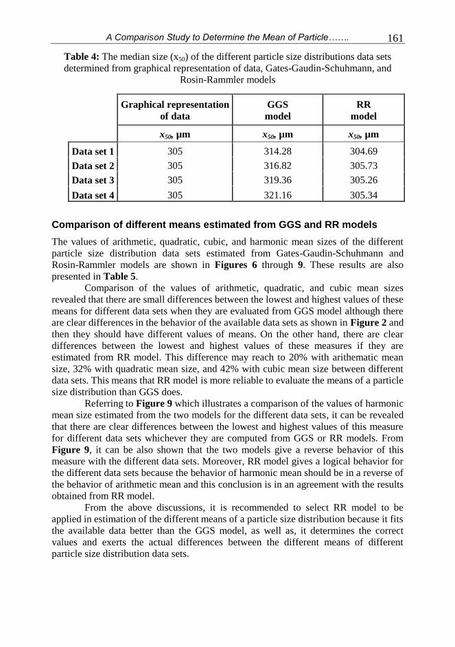
Table 4: The median size (x50) of the different particle size distributions data sets

determined from graphical representation of data, Gates-Gaudin-Schuhmann, and

Rosin-Rammler models

Graphical representation

of data

GGS

model

RR

model

x50, µm x50, µm x50, µm

Data set 1 305 314.28 304.69

Data set 2 305 316.82 305.73

Data set 3 305 319.36 305.26

Data set 4 305 321.16 305.34

Comparison of different means estimated from GGS and RR models

The values of arithmetic, quadratic, cubic, and harmonic mean sizes of the different

particle size distribution data sets estimated from Gates-Gaudin-Schuhmann and

Rosin-Rammler models are shown in Figures 6 through 9. These results are also

presented in Table 5.

Comparison of the values of arithmetic, quadratic, and cubic mean sizes

revealed that there are small differences between the lowest and highest values of these

means for different data sets when they are evaluated from GGS model although there

are clear differences in the behavior of the available data sets as shown in Figure 2 and

then they should have different values of means. On the other hand, there are clear

differences between the lowest and highest values of these measures if they are

estimated from RR model. This difference may reach to 20% with arithematic mean

size, 32% with quadratic mean size, and 42% with cubic mean size between different

data sets. This means that RR model is more reliable to evaluate the means of a particle

size distribution than GGS does.

Referring to Figure 9 which illustrates a comparison of the values of harmonic

mean size estimated from the two models for the different data sets, it can be revealed

that there are clear differences between the lowest and highest values of this measure

for different data sets whichever they are computed from GGS or RR models. From

Figure 9, it can be also shown that the two models give a reverse behavior of this

measure with the different data sets. Moreover, RR model gives a logical behavior for

the different data sets because the behavior of harmonic mean should be in a reverse of

the behavior of arithmetic mean and this conclusion is in an agreement with the results

obtained from RR model.

From the above discussions, it is recommended to select RR model to be

applied in estimation of the different means of a particle size distribution because it fits

the available data better than the GGS model, as well as, it determines the correct

values and exerts the actual differences between the different means of different

particle size distribution data sets.


2 5 0

3 0 0

3 5 0

4 0 0


Ar

ith

me

tic

me

an

siz

e,

µm

G G S mo de l

R R mo de l

Fig. 6: Comparison of the values of arithmetic mean size estimated from Gates-

Gaudin-Schuhmann and Rosin-Rammler models for the different data sets

2 5 0

3 0 0

3 5 0

4 0 0

4 5 0

5 0 0


Qu

ad

ra

tic

me

an

siz

e,

µm G G S mo de l

R R mo de l

Fig. 7: Comparison of the values of quadratic mean size estimated from Gates-Gaudin-

Schuhmann and Rosin-Rammler models for the different data sets

2 5 0

3 0 0

3 5 0

4 0 0

4 5 0

5 0 0

5 5 0

6 0 0


Cu

bic

me

an

siz

e,

µm

G G S mo de l

R R mo de l

Fig. 8: Comparison of the values of cubic mean size estimated from Gates-Gaudin-



0

5 0

1 0 0

1 5 0

2 0 0

2 5 0

3 0 0

3 5 0

4 0 0


Ha

rm

on

ic m

ea

n s

ize

, µ

m

G G S mo de l

R R mo de l

Fig. 9: Comparison of the values of harmonic mean size estimated from Gates-Gaudin-


Table 5: The values of arithmetic, quadratic, cubic, and harmonic means of the

different particle size distribution data sets estimated from Gates-Gaudin-Schuhmann

and Rosin-Rammler models

Arithmetic

mean

size, µm

Quadratic mean

size, µm

Cubic mean

size, µm

Harmonic

mean

size, µm

GGS RR GGS RR GGS RR GGS RR

Data set 1 313.69 379.19 361.63 487.99 394.27 586.80 6.06 358.95

Data set 2 304.84 341.92 337.96 409.94 361.07 467.25 128.91 268.90

Data set 3 302.87 321.28 327.57 371.06 345.24 409.64 188.14 194.06

Data set 4 303.25 311.57 323.91 354.18 338.93 384.94 214.17 149.36

CONCLUSIONS

The following conclusions may be drawn from this research:

1. The different means (arithmetic, quadratic, cubic, geometric, and harmonic) of a

particle size distribution can be easily estimated using Gates-Gaudin-Schuhmann

and Rosin-Rammler models.

2. The two models provide a very good representation for all the available data sets

although the RR model provides a better fit to the data than GGS does.

3. There are small differences between the values of different means for different data

sets when they are evaluated from GGS model.

4. There are clear differences between the lowest and highest values of arithmetic,

quadratic, and cubic means of different data sets if they are estimated from RR

model. This difference may reach to 20% with arithematic mean size, 32% with

quadratic mean size, and 42% with cubic mean size.


5. There are clear differences between the lowest and highest values of harmonic

mean for different data sets whichever they are computed from GGS or RR

models. The two models give a reverse behavior of this measure with the different

data sets.

6. It is recommended to select RR model to be applied in estimation of the different

means of a particle size distribution because it fits the available data better than the

GGS model, as well as, it determines the correct values and exerts the actual

differences between the different means of different particle size distribution data

sets.

REFERENCES

1. Svarovsky, L., Characterization of particles suspended in liquids, In: Solid-

Liquid Separation, Butterworth-Heinemann, Oxford, England, 4th ed., Ch. 2, pp.

30-65, (2000).

2. Djamarani, K.M. and Clark, I.M., Characterization of particle size based on fine

and coarse fractions, Powder Technology, Vol. 93, pp. 101-108, (1997).

3. Garcia, A.M., Cuerda-Correa, E.M. and Diaz-Diez, M.A., Application of the

Rosin-Rammler and Gates-Gaudin-Schuhmann models to the particle size

distribution analysis of agglomerated coke, Materials Characterization, Vol. 52,

pp. 159-164, (2004).

4. Hsih, C.S., Wen, S.B. and Kuan, C.C., An exposure model for valuable

components in comminuted particles, Int. J. Mineral Process., Vol. 43, pp. 145-

165, (1995).

5. Wills, B.A., Particle size analysis, In: Mineral Processing Technology, Pergamon

Press, Oxford, England, 5th ed., Ch. 4, pp. 181-225, (1992).

6. Teipel, U., Leisinger, K. and Mikonsaari, I., Comminution of crystalline material

by ultrasonics, Int. J. Mineral Process., Vol. 74S, pp. S183-190, (2004).

7. Wen, S.B., Hsih, C.S. and Kuan, C.C., The application of a mineral exposure

model in a gold leaching operation, Int. J. Mineral Process., Vol. 46, pp. 215-230,

(1996).

8. Fuerstenau, D.W., Kapur, P.C., Schoenert, K. and Marktscheffel, M., Comparison

of energy consumption in the breakage of single particles in a rigidly mounted roll

mill with ball mill grinding, Int. J. Mineral Process., Vol. 28, pp. 109-125, (1990).

9. Kapur, P.C. and Fuerstenau, D.W., Energy-size reduction laws revisited, Int. J.

Mineral Process., Vol. 20, pp. 45-57, (1987).

10. Shook, C.A. and Roco, M.C., Basic concepts for single-phase fluids and

particles, In: Slurry Flow (Principles and Practice), Butterworth-Heinemann,

Boston, U.S.A., Ch. 1, pp. 1-25, (1991).

11. Fang, Z., Patterson, B.R. and Turner, M.E., Modeling particle size distribution by

the Weibull distribution function, Materials Characterization, Vol. 31, pp. 177-

182, (1993).

12. Xiang, Y. Zhang, J. and Liu, C., Verification for particle size distribution of

ultrafine powders by the SAXS method, Materials Characterization, Vol. 44, pp.

435-439, (2000).


13. Dierickx, D., Basu, B., Vleugels, J. and Van der Biest, O., Statistical extreme

value modeling of particle size distributions: experimental grain size distribution

type estimation and parameterization of sintered zirconia, Materials

Characterization, Vol. 45, pp. 61-70, (2000).

14. Ramakrishnan, K.N., Investigation of the effect of powder particle size

distribution on the powder microstructure and mechanical properties of

consolidated material made from a rapidly solidified Al, Fe, Ce alloy powder: part

I. Powder microstructure, Materials Characterization, Vol. 33, pp. 119-128,

(1994).

15. Ramakrishnan, K.N., Investigation of the effect of powder particle size

distribution on the powder microstructure and mechanical properties of

consolidated material made from a rapidly solidified Al, Fe, Ce alloy powder: part

II. Mechanical properties, Materials Characterization, Vol. 33, pp. 129-134,

(1994).

16. Rao, S.S., Stochastic programming, In: Engineering Optimization (Theory and

Practice), New Age International (P) Limited, New Delhi, India, 3rd ed., Ch. 11,

pp. 715-767, (2004).

17. Kheifets, A.S. and Lin, I.J., Energetic approach to kinetics of batch ball milling,

Int. J. Mineral Process., Vol. 54, pp. 81-97, (1998).

18. Wu, S.Z., Chau, K.T. and Yu, T.X., Crushing and fragmentation of brittle spheres

under double impact test, Powder Technology, Vol. 143-144, pp. 41-55, (2004).

19. Mu, Y., Lyddiatt, A. and Pacek, A.W., Manufacture by water/oil emulsification of

porous agarose beads: effect of processing conditions on mean particle size, size

distribution and mechanical properties, Chemical Eng. and Process, Vol. 44, pp.

1157-1166, (2005).

20. Lech, M., Polednia, E. and Werszler, A., Measurement of solid mean particle size

using tomography, Powder Technology, Vol. 111, pp. 186-191, (2000).

21. Ouchiyama, N., Rough, S.L. and Bridgwater, J., A population balance approach to

describing bulk attrition, Chemical Eng. Science, Vol. 60, pp. 1429-1440, (2005).

22. Gbor, P.K. and Jia, C.Q., Critical evaluation of coupling particle size distribution

with the shrinking core model, Chemical Eng. Science, Vol. 59, pp. 1979-1987,

(2004).

23. Choi, W.S., Chung, H.Y., Yoon, B.R. and Kim, S.S., Applications of grinding

kinetics analysis to fine grinding characteristics of some inorganic materials using

composite grinding media by planetary ball mill, Powder Technology, Vol. 115,

pp. 209-214, (2001).

24. Hosten, C. and San, O., Reassessment of correlations for the dewatering

characteristics of filter cakes, Minerals Engineering, Vol. 15, pp. 347-353, (2002).

25. Stamboliadis, E.Th., A contribution to the relationship of energy and particle size

in the comminution of brittle particulate materials, Minerals Engineering, Vol. 15,

pp. 707-713, (2002).

26. Cheong, Y.S., Reynolds, G.K., Salman, A.D. and Hounslow, M.J., Modeling

fragment size distribution using two-parameter Weibull equation, Int. J. Mineral

Process., Vol. 74S, pp. S227-S237, (2004).


دراسة مقارنة لتحديد متوسط حجم الحبيبات بغرض عمل توصيف حقيقي للبيانات بيئةالمتعلقة بال

البيئية هي الحصول على توزيع كمي ونوعي دقيق للملوثات حيث أن هذه تأحد أهم المراحل في الدراسا الدراسات تتطلب حساب حجم الحبيبات بدقة عالية.

وهاااو حجاام المنطاال المناااارر لنساابة ماارور تراكمياااة (x50)هناااا الكثياار ماان البااااحثين يسااتطدمون الوساايط كمقاييس لتقييم توزيع الحجم 05لمنطل المنارر لنسبة مرور تراكمية %وهو حجم ا (x80)أو حتى %05

للحبيبااات والتااي تنااتل ماان اللمليااات المطتليااة مثاال عمليااة التكساايرا الطحاانا التصااني ا الترساايبا فصاال المواد الصلبة عن السائلةا أو حتى اللمليات الناتجة عن تقييم أو دراسة شكل وتوزيع الملوث.

ييس ليسااات دقيقاااة بدرجاااة كافياااة حتاااى يمكااان التيرياااق باااين التوزيلاااات المطتلياااة لحجااام غيااار أن هاااذه المقاااا أو كليهما. x80أو x50الحبيبات ألن كثير من التوزيلات ربما يكون لها نيس القيمة من

بصاورة دقيقاة (MPSD)هذا البحث يلتبر محاولة للمل منهجية جديدة لتحديد الحجم المتوسط للحبيباات . القاااايم المحسااااوبة لهااااذه Rosin-Rammlerو Gates-Gaudin-Schuhmannجي بإسااااتطدام نمااااوذ

المقاييس تأطذ في اإلعتبار ليس فقط األحجام اليردية للحبيبات ولكن أيضا النسب الوزنية المناررة لهم. (x50)وقد أرهرت نتائل هذا البحث أن التوزيلات المطتلية ألحجام الحبيبات والتي لها نيس قيمة الوسيط

وطصوصاااا عناااد مساااتطدام ملادلاااة (MPSD)تلطاااى قااايم مطتلياااة للمقيااااس المساااتطدم فاااي هاااذا البحاااث Rosin-Rammler.

فاي هااذا البحاث تاام أيضاا الحصااول علاى تلبياارات رياضاية بساايطة والتاي ماان طجلهاا أمكاان حسااب الحجاام قي وذلاااا عنااااد المتوساااط للحبيباااات ساااوات كاااان المتوساااط الرياضاااايا التكليبااايا الهندسااايا أو حتاااى التاااواف

مستطدام أي من النموذجين المشار مليهم سابقا.عناد حسااب الحجام Rosin-Rammlerووفقا للنتائل التي توصل مليهاا البحاث نوصاى باساتطدام نماوذ

-Gates-Gaudinالمتوسااط للحبيبااات حيااث أن هااذا النمااوذ يوفااق البيانااات بصااورة أفضاال ماان نمااوذ

Schuhmann طجلا حساااب القايم الصااحيحة وتليااين اليروقاات اليلليااة بااين وفاي نيااس الوقات يمكاان ماان المتوسطات المطتلية للبيانات.

ويلااد هااذا البحاااث الجاازت األول ماان دراساااة سااو تتبااع بلمااال دراسااة حالااة حقيقياااة لبيانااات فلليااة مرتبطاااة بالبيئة.

Documents

M.M. Ahmed and S.S. Ahmed Mining and Metallurgical ... of Engineering Sciences, Assiut University, Vol. 36, No. 1, pp. 147- 166, January 2008 147 A COMPARISON STUDY TO DETERMINE THE