Mixture Ratio and Thrust Control of a Liquid-Propellant ... · PDF fileMixture Ratio and Thrust Control of a Liquid-Propellant ... 1.1.1 Controlled Engines and Reusable Rockets

Mixture Ratio and Thrust Control of a Liquid-PropellantRocket Engine

Henrique Coxinho Tomé Raposo

Thesis to obtain the Master of Science Degree in

Aerospace Engineering

Supervisor: Eng. Elisa Cliquet Moreno

Dr. António Manuel dos Santos Pascoal

Examination Committee

Chairperson: Dr. João Manuel Lage de Miranda Lemos

Supervisor: Dr. António Manuel dos Santos Pascoal

Member of the Committee: Dr. Luís Manuel Braga da Costa Campos

November 2016

ii

Resumo

Atualmente a maioria dos motores de foguetoes europeus funcionam em anel aberto. Para obter

uma determinada forca propulsiva e racio de consumo de combustıveis e necessario ajustar a seccao das

valvulas que controlam o caudal dos combustıveis antes de cada voo. Na pratica, este procedimento

limita o desempenho porque existem um conjunto de perturbacoes externas que atuam sobre o motor

ao longo do voo, o que se traduz na deriva do ponto de equilıbrio. A dispersao e a imprevisibilidade

associada a esta deriva tem um impacto negativo sobre a quantidade de combustıveis embarcados para

assegurar o sucesso da missao. O presente trabalho implementa um controlador em anel fechado para

o motor VINCI, tendo por objetivo assegurar a manutencao de um ponto de equilıbrio otimo nominal

assim como a transicao para um regime a 70% da forca propulsiva nominal. Primeiramente, obtem-se um

modelo linear reduzido a cinco estados do ciclo termodinamico expander, combinando uma abordagem

analıtica de linearizacao e um metodo de identificacao de mınimos quadrados. Dois controladores PID

sao ajustados com base nos pares input-output que minimizam os efeitos de acoplagem. Modificacoes

tais como feed-forward, anti-windup e tratamento das medidas dos sensores sao realizadas de forma a

respeitar as especificacoes. Simulacoes efetuadas no modelo nao-linear indicam que um unico controlador

e suficientemente robusto para realizar a transicao entre regimes. Este trabalho confirma a aplicabilidade

de um controlador PID modificado a um motor naturalmente estavel e estabelece a base para o estudo

da dinamica dominante de outros ciclos termodinamicos.

Palavras-chave: VINCI, Ciclo termodinamico expander, Controlo de forca propulsiva, Con-

trolo de racio de mistura, PID

iii

iv

Abstract

Presently, most European launchers’ engines work in open-loop. Not only does this oblige the valves

which regulate the mass flow-rates to be calibrated before flight in order to obtain a desired thrust and

mixture ratio, but it also limits performance. Varying operating conditions translate into a drifting

equilibrium point. The associated dispersion forces us to carry extra propellants to ensure mission

success. The present work implements a closed-loop controller on the VINCI engine, which aims to

maintain an optimal nominal equilibrium point despite external perturbations, and also to transition to

a 70% thrust regime. To meet these objectives, a reduced linear model of the expander thermodynamic

cycle of the engine is obtained through a combination of an analytic linearization approach and a least-

squares identification method. A sensitivity study confirms that 5 states suffice to describe the dominant

dynamics. Two PID controllers are tuned based on the input-output pairings that minimize coupling

within the 2 × 2 MIMO system. Modifications such as feed-forward, anti-windup and measurements

filtering are made in order to match the control specifications. Simulations on the non-linear model

indicate a single controller to be both capable of maintaining an operating point and of transitioning

to the low-thrust regime, all while attenuating perturbations. Robustness to parameter uncertainty is

assessed and preliminary results indicate actuator saturation before the controller displays any signs of

instability. This work confirms the applicability of a modified PID controller to a naturally stable engine

and lays the foundation to the study of other thermodynamic cycles.

Keywords: VINCI, Expander thermodynamic cycle, Thrust control, Mixture-ratio control, PID

v

vi

Contents

Resumo . . . . . . . . . . . . . . . . . . . . . . . . . . . . . . . . . . . . . . . . . . . . . . . . . iii

Abstract . . . . . . . . . . . . . . . . . . . . . . . . . . . . . . . . . . . . . . . . . . . . . . . . . v

List of Tables . . . . . . . . . . . . . . . . . . . . . . . . . . . . . . . . . . . . . . . . . . . . . . xi

List of Figures . . . . . . . . . . . . . . . . . . . . . . . . . . . . . . . . . . . . . . . . . . . . . xiii

Nomenclature . . . . . . . . . . . . . . . . . . . . . . . . . . . . . . . . . . . . . . . . . . . . . . xv

Glossary . . . . . . . . . . . . . . . . . . . . . . . . . . . . . . . . . . . . . . . . . . . . . . . . . xix

1 Introduction 1

1.1 Historical Background . . . . . . . . . . . . . . . . . . . . . . . . . . . . . . . . . . . . . . 1

1.1.1 Controlled Engines and Reusable Rockets . . . . . . . . . . . . . . . . . . . . . . . 2

1.2 Motivation . . . . . . . . . . . . . . . . . . . . . . . . . . . . . . . . . . . . . . . . . . . . 3

1.3 Objectives . . . . . . . . . . . . . . . . . . . . . . . . . . . . . . . . . . . . . . . . . . . . . 5

1.4 Previous Work . . . . . . . . . . . . . . . . . . . . . . . . . . . . . . . . . . . . . . . . . . 5

1.5 Thesis Outline . . . . . . . . . . . . . . . . . . . . . . . . . . . . . . . . . . . . . . . . . . 7

2 Liquid-propellant Engines 9

2.1 Propulsion Fundamentals . . . . . . . . . . . . . . . . . . . . . . . . . . . . . . . . . . . . 9

2.2 Engine Work Principle and Classification . . . . . . . . . . . . . . . . . . . . . . . . . . . 12

2.2.1 Liquid Propellants . . . . . . . . . . . . . . . . . . . . . . . . . . . . . . . . . . . . 14

2.3 Summary . . . . . . . . . . . . . . . . . . . . . . . . . . . . . . . . . . . . . . . . . . . . . 14

3 Elements of Control Theory 17

3.1 State-space Model Linearization . . . . . . . . . . . . . . . . . . . . . . . . . . . . . . . . . 17

3.2 Model Identification . . . . . . . . . . . . . . . . . . . . . . . . . . . . . . . . . . . . . . . 18

3.2.1 Least-squares Method . . . . . . . . . . . . . . . . . . . . . . . . . . . . . . . . . . 19

3.3 Reduction Methods . . . . . . . . . . . . . . . . . . . . . . . . . . . . . . . . . . . . . . . . 20

3.3.1 Matched DC Gain Method . . . . . . . . . . . . . . . . . . . . . . . . . . . . . . . 20

3.4 Controllability and Observability . . . . . . . . . . . . . . . . . . . . . . . . . . . . . . . . 21

3.4.1 Controllability and Observability Matrices . . . . . . . . . . . . . . . . . . . . . . . 21

3.5 Singular Values and Modulus Margin . . . . . . . . . . . . . . . . . . . . . . . . . . . . . . 22

3.6 Robustness Analysis . . . . . . . . . . . . . . . . . . . . . . . . . . . . . . . . . . . . . . . 24

3.7 Summary . . . . . . . . . . . . . . . . . . . . . . . . . . . . . . . . . . . . . . . . . . . . . 25

vii

4 VINCI Engine 27

4.1 Introduction . . . . . . . . . . . . . . . . . . . . . . . . . . . . . . . . . . . . . . . . . . . . 27

4.2 Thermodynamic Cycle . . . . . . . . . . . . . . . . . . . . . . . . . . . . . . . . . . . . . . 28

4.3 Mixture Ratio and Thrust Control Valves . . . . . . . . . . . . . . . . . . . . . . . . . . . 29

4.4 VINCI Governing Equations Linearization . . . . . . . . . . . . . . . . . . . . . . . . . . . 31

4.4.1 State-space Model Assembly . . . . . . . . . . . . . . . . . . . . . . . . . . . . . . 32

4.5 Summary . . . . . . . . . . . . . . . . . . . . . . . . . . . . . . . . . . . . . . . . . . . . . 33

5 Model Implementation 35

5.1 Analytical Model . . . . . . . . . . . . . . . . . . . . . . . . . . . . . . . . . . . . . . . . . 35

5.1.1 Complete Model . . . . . . . . . . . . . . . . . . . . . . . . . . . . . . . . . . . . . 36

5.1.2 Reduced Model . . . . . . . . . . . . . . . . . . . . . . . . . . . . . . . . . . . . . . 37

5.2 Identified Model . . . . . . . . . . . . . . . . . . . . . . . . . . . . . . . . . . . . . . . . . 38

5.2.1 Complete Model . . . . . . . . . . . . . . . . . . . . . . . . . . . . . . . . . . . . . 39

5.2.2 Reduced Model . . . . . . . . . . . . . . . . . . . . . . . . . . . . . . . . . . . . . . 40

5.2.3 Controllability and Observability . . . . . . . . . . . . . . . . . . . . . . . . . . . . 43

5.3 Model Comparison . . . . . . . . . . . . . . . . . . . . . . . . . . . . . . . . . . . . . . . . 44

5.4 Model Analysis . . . . . . . . . . . . . . . . . . . . . . . . . . . . . . . . . . . . . . . . . . 46

5.4.1 Turbo-pump Moment of Inertia . . . . . . . . . . . . . . . . . . . . . . . . . . . . . 46

5.4.2 Regenerative Circuit . . . . . . . . . . . . . . . . . . . . . . . . . . . . . . . . . . . 47

5.4.3 Hydrogen Injection Cavity . . . . . . . . . . . . . . . . . . . . . . . . . . . . . . . . 49

5.4.4 Mode Analysis Summary . . . . . . . . . . . . . . . . . . . . . . . . . . . . . . . . 50

5.5 Summary . . . . . . . . . . . . . . . . . . . . . . . . . . . . . . . . . . . . . . . . . . . . . 50

6 Control Specifications 51

6.1 Transient and Steady-State Time-Response . . . . . . . . . . . . . . . . . . . . . . . . . . 51

6.2 Stability margins . . . . . . . . . . . . . . . . . . . . . . . . . . . . . . . . . . . . . . . . . 52

6.3 Discretization Frequency . . . . . . . . . . . . . . . . . . . . . . . . . . . . . . . . . . . . . 52

6.4 Sensor’s Characteristics . . . . . . . . . . . . . . . . . . . . . . . . . . . . . . . . . . . . . 52

6.5 Parameter Uncertainty . . . . . . . . . . . . . . . . . . . . . . . . . . . . . . . . . . . . . . 53

6.6 Domain Variation of the Input Perturbations . . . . . . . . . . . . . . . . . . . . . . . . . 53

6.7 Mechanical and Thermal Bounds . . . . . . . . . . . . . . . . . . . . . . . . . . . . . . . . 53

6.8 Failure Events . . . . . . . . . . . . . . . . . . . . . . . . . . . . . . . . . . . . . . . . . . . 54

6.9 Summary . . . . . . . . . . . . . . . . . . . . . . . . . . . . . . . . . . . . . . . . . . . . . 54

7 Control Law Design and Implementation 55

7.1 PID Controller . . . . . . . . . . . . . . . . . . . . . . . . . . . . . . . . . . . . . . . . . . 55

7.2 PID Controller Design with the Reduced Linear Model . . . . . . . . . . . . . . . . . . . . 58

7.3 Effect of the Valve’s Dynamic Model . . . . . . . . . . . . . . . . . . . . . . . . . . . . . . 59

7.4 Performance Evaluation on the Complete Linear Model and Measurement Noise Effect . . 60

viii

7.4.1 Simulink Diagram . . . . . . . . . . . . . . . . . . . . . . . . . . . . . . . . . . . . 62

7.4.2 Closed-loop Poles . . . . . . . . . . . . . . . . . . . . . . . . . . . . . . . . . . . . . 62

7.4.3 Modulus Margin . . . . . . . . . . . . . . . . . . . . . . . . . . . . . . . . . . . . . 63

7.4.4 Frequency Response . . . . . . . . . . . . . . . . . . . . . . . . . . . . . . . . . . . 64

7.5 Summary . . . . . . . . . . . . . . . . . . . . . . . . . . . . . . . . . . . . . . . . . . . . . 65

8 Results 67

8.1 Flight Simulation on the CARINS Non-linear Model . . . . . . . . . . . . . . . . . . . . . 67

8.1.1 Energy Consumption . . . . . . . . . . . . . . . . . . . . . . . . . . . . . . . . . . . 68

8.2 Robustness to Parameter Uncertainty . . . . . . . . . . . . . . . . . . . . . . . . . . . . . 71

8.2.1 Complete Linear Model . . . . . . . . . . . . . . . . . . . . . . . . . . . . . . . . . 71

8.2.2 Non-Linear Model . . . . . . . . . . . . . . . . . . . . . . . . . . . . . . . . . . . . 75

8.2.3 Failure cases . . . . . . . . . . . . . . . . . . . . . . . . . . . . . . . . . . . . . . . 77

8.3 Summary . . . . . . . . . . . . . . . . . . . . . . . . . . . . . . . . . . . . . . . . . . . . . 78

9 Conclusion and Future Work 79

9.1 Conclusion . . . . . . . . . . . . . . . . . . . . . . . . . . . . . . . . . . . . . . . . . . . . 79

9.2 Future Work . . . . . . . . . . . . . . . . . . . . . . . . . . . . . . . . . . . . . . . . . . . 80

Bibliography 81

A Engine State Admissible Bounds 83

ix

x

List of Tables

4.1 Vinci engine nominal equilibrium point. . . . . . . . . . . . . . . . . . . . . . . . . . . . . 28

4.2 Characteristics of the ISFM valves (brushless motor) - confidential data. . . . . . . . . . . 30

4.3 Number of states, inputs and outputs of the analytic linear model. . . . . . . . . . . . . . 33

5.1 Input-output equilibrium values at 130kN. . . . . . . . . . . . . . . . . . . . . . . . . . . . 35

5.2 Poles of the reduced analytical linear model. . . . . . . . . . . . . . . . . . . . . . . . . . . 37

5.3 Poles of the reduced identified linear model. . . . . . . . . . . . . . . . . . . . . . . . . . . 40

5.4 Zeros of the reduced identified linear model. . . . . . . . . . . . . . . . . . . . . . . . . . . 40

5.5 2% range settling times of the non-linear model. . . . . . . . . . . . . . . . . . . . . . . . 41

5.6 Controllability and observability matrix ranks of the identified models. . . . . . . . . . . . 43

5.7 Settling times for varying turbo-pump moment of inertia. . . . . . . . . . . . . . . . . . . 47

5.8 Poles of the reduced identified linear model after a decrease of 50% of the heat capacity of

the interface wall between the regenerative circuit and the combustion chamber. . . . . . 48

5.9 Zeros of the reduced identified linear model after a decrease of 50% of the heat capacity of

the interface wall between the regenerative circuit and the combustion chamber. . . . . . 48

5.10 Poles of the reduced identified linear model after an increase of 50% of the heat capacity

of the interface wall between the regenerative circuit and the combustion chamber. . . . . 49

5.11 Zeros of the reduced identified linear model after an increase of 50% of the heat capacity

of the interface wall between the regenerative circuit and the combustion chamber. . . . . 49

7.1 Gain and phase margins for each transfer function of the closed-loop. . . . . . . . . . . . . 64

8.1 Studied uncertain parameters. . . . . . . . . . . . . . . . . . . . . . . . . . . . . . . . . . . 72

8.2 Robustness limits to failure events. . . . . . . . . . . . . . . . . . . . . . . . . . . . . . . . 77

xi

xii

List of Figures

1.1 Fuel consumption during flight. . . . . . . . . . . . . . . . . . . . . . . . . . . . . . . . . . 4

1.2 Block diagram of the controlled system . . . . . . . . . . . . . . . . . . . . . . . . . . . . . 4

2.1 General engine design and its main subsystems (image courtesy of Snecma). . . . . . . . . 13

4.1 VINCI’s synoptic (image extracted from [24]) . . . . . . . . . . . . . . . . . . . . . . . . . 29

4.2 VBPH Simulink block diagram . . . . . . . . . . . . . . . . . . . . . . . . . . . . . . . . . 30

5.1 Linear and non-linear models time-response comparison to a VBPH section step of 20% of

the nominal value at t = 0. . . . . . . . . . . . . . . . . . . . . . . . . . . . . . . . . . . . 36

5.2 Linear and non-linear models time-response comparison to a VBPO section step of 10% of

the nominal value at t = 0.25. . . . . . . . . . . . . . . . . . . . . . . . . . . . . . . . . . . 36

5.3 Full and reduced linear models time-response comparison to a VBPH section step of 20%

of the nominal value at t = 0. . . . . . . . . . . . . . . . . . . . . . . . . . . . . . . . . . . 38

5.4 Full and reduced linear models time-response comparison to a VBPO section step of 10%

of the nominal value at t = 0. . . . . . . . . . . . . . . . . . . . . . . . . . . . . . . . . . . 38

5.5 Full identified linear model and non-linear model time-response comparison to a VBPH

section step of 1% of the nominal value at t = 0 and a VBPO section step of 1% of the

nominal value at t = 0.25 . . . . . . . . . . . . . . . . . . . . . . . . . . . . . . . . . . . . . 39

5.6 Reduced identified linear model and non-linear model time-response comparison to a VBPH











nominal value at t = 0.25 around the 130kN equilibrium point. . . . . . . . . . . . . . . . 43

5.10 Bode plots of the five models for a VBPH input. . . . . . . . . . . . . . . . . . . . . . . . 45

xiii

5.11 Bode plots of the five models for a VBPO input. . . . . . . . . . . . . . . . . . . . . . . . 45

5.12 VBPH (t = 0) and VBPO (t = 0.5) step time-responses for turbo-pump systems with

different moments of inertia. . . . . . . . . . . . . . . . . . . . . . . . . . . . . . . . . . . . 46

5.13 VBPH and VBPO step time-responses for interface walls with different heat capacities. . 48

5.14 VBPH and VBPO step time-responses for hydrogen injection cavities with different volumes. 49

6.1 Block diagram of the sensors. . . . . . . . . . . . . . . . . . . . . . . . . . . . . . . . . . . 53

7.1 PID block diagram. . . . . . . . . . . . . . . . . . . . . . . . . . . . . . . . . . . . . . . . . 56

7.2 Bode plots of the scaled open-loop transfer functions. . . . . . . . . . . . . . . . . . . . . . 57

7.3 Time response to a step of mixture ratio (MR = −1 at t = 1/6). . . . . . . . . . . . . . . 58

7.4 Time response to a step of mixture ratio (MR = −1 at t = 1/6). . . . . . . . . . . . . . . 59

7.5 Output time response to a step of mixture ratio (MR = −1 at t = 0.2) on the complete

linear model. . . . . . . . . . . . . . . . . . . . . . . . . . . . . . . . . . . . . . . . . . . . 60

7.6 Input time response to a step of mixture ratio (MR = −1 at t = 0.2) on the complete

linear model. . . . . . . . . . . . . . . . . . . . . . . . . . . . . . . . . . . . . . . . . . . . 61

7.7 Scaled bode plot of the diagonal transfer functions of the closed loop system. . . . . . . . 61

7.8 Input time response to a step of mixture ratio of MR = −1 at t = 1/6 on the complete

linear model with measurement noise. . . . . . . . . . . . . . . . . . . . . . . . . . . . . . 61

7.9 Closed-loop block diagram. . . . . . . . . . . . . . . . . . . . . . . . . . . . . . . . . . . . 62

7.10 Pole-zero maps of the closed-loop system. . . . . . . . . . . . . . . . . . . . . . . . . . . . 63

7.11 Maximum and minimum singular values of I +GK. . . . . . . . . . . . . . . . . . . . . . 63

7.12 Maximum and minimum singular values of the closed-loop transfer functions. . . . . . . . 65

8.1 Output references during flight simulation. . . . . . . . . . . . . . . . . . . . . . . . . . . . 68

8.2 Non-linear system flight simulation results. . . . . . . . . . . . . . . . . . . . . . . . . . . 69

8.3 Valve consumption comparison when adding a deadzone to the error signals. . . . . . . . 70

8.4 Non-linear system flight simulation results with a dead-band associated to the setpoint error. 70

8.5 Output references during flight simulation. . . . . . . . . . . . . . . . . . . . . . . . . . . . 71

8.6 Relative frequency histograms of the performance parameters. . . . . . . . . . . . . . . . . 73

8.7 Relative frequency histograms of the performance parameters. . . . . . . . . . . . . . . . . 74

8.8 PID with anti-windup block diagram. . . . . . . . . . . . . . . . . . . . . . . . . . . . . . 75

8.9 Non-linear system flight simulation results for the worst-cases. . . . . . . . . . . . . . . . . 76

8.10 Non-linear system flight simulation results with failure event. . . . . . . . . . . . . . . . . 78

A.1 Nominal non-linear system flight simulation results. . . . . . . . . . . . . . . . . . . . . . 83

A.2 Non-linear system flight simulation results for the worst-cases among the uncertainty set. 84

xiv

Nomenclature

Propulsion: Roman symbols

Cd Flow coefficient.

Cw Wall specific heat capacity.

F Thrust.

g0 Acceleration of gravity at sea level.

Is Specific impulse.

J Moment of inertia.

kp Pressure loss coefficient.

L Length.

m Mass flow rate.

MR Mixture ratio.

p Static pressure.

Pchem Available chemical power.

Pkin Available kinetic power.

Pthermal Available thermal power.

QR Available energy per unit mass of chemical propellant.

R Ideal gas constant.

S Open section.

T Temperature.

V Volume.

v Gas ejection velocity relative to the vehicle.

Propulsion: Greek symbols

η Efficiency.

Φ Heat flux.

κ Real gas specific heat ratio.

ρ Density.

Control systems: Roman symbols

A,B,C,D Linear state-space representation matrices.

Ai, Ao Input and output signal amplitude.

fi i-th state function of a state-space representation.

xv

G(s) Plant model transfer matrix.

gi i-th output function of a state-space representation.

I Identity matrix.

j Imaginary unit.

K(s) Controller transfer matrix.

L(s) Open-loop transfer matrix.

L[t0,t1](u(t)) Reachability map.

m Number of inputs of a state-space model.

n Number of states of a state-space model.

p Number of outputs of a state-space model.

r Modulus margin.

R(s) Relative gain array.

S(s) Output sensitivity transfer matrix.

t Time.

U Matrix of output singular vectors.

ui i-th input of a state-space representation.

uk Input vector at instant k.

V Matrix of input singular vectors.

xi i-th state of a state-space representation.

xk State vector at instant k.

xr, xnr Subset of states to be truncated and to be kept, respectively.

yi i-th output of a state-space representation.

yk Output vector at instant k.

Control systems: Greek symbols

αi(t) Scalar time functions of the series expansion of the exponential function.

∆ Variational quantity with respect to an equilibrium point (vector operator).

δ Variational quantity with respect to an equilibrium point (scalar operator).

ω Angular frequency.

σ Maximum singular value.

Σ Singular value matrix from the singular value decomposition.

σ Singular value.

¯σ Minimum singular value.

θ Geometric open angle of a valve.

Superscripts

−1 Matrix inverse.

x Steady-state value.

x Time derivative.

H Hermitian transpose or conjugate transpose.

x Scaled vector.

xvi

T Transpose.

Subscripts

0 Steady-state quantity.

atm Atmospheric.

chmb Combustion chamber.

comb Combustion process.

exp Gas expansion and ejection process.

e Inlet.

fuel Fuel.

g Geometric.

hyd Hydraulic.

H Hydrogen.

injH Hydrogen injector.

nozzle At the exit of the nozzle of the engine.

oxi Oxidizer.

O Oxygen.

P Pump.

scl Scaling matrix.

s Outlet.

T Turbine.

t Nozzle throat.

xvii

xviii

Glossary

CARINS Unsteady Network Calculator (Calculateur de

Reseaux Instationnaires).

CNES Centre National d’Etudes Spatiales.

DF Describing Function.

LH2 Liquid Hydrogen.

LMDE Lunar Module Descent Engine.

LOX Liquid Oxygen.

LPRE Liquid-Propellant Rocket Engine.

MIMO Multiple Input Multiple Output.

MR Mixture Ratio.

PAM Propellant Active Management System.

PCC Combustion Chamber Pressure.

PEP Pump Inlet Pressure.

PID Proportional Integral Derivative.

SISO Single Input Single Output.

SSME Space Shuttle Main Engine.

SVD Singular Value Decomposition.

TEP Pump Inlet Temperature.

TPH Hydrogen Turbo-pump.

TPO Oxygen Turbo-pump.

TVC Thrust-vector Control System.

VBPH Hydrogen By-pass Valve.

VBPO Oxygen By-pass Valve.

xix

xx

Chapter 1

Introduction

1.1 Historical Background

To this day it is still unclear when the first true rockets appeared. Throughout more than 2000

years various cultures have experimented with propulsive devices, often by accident. One of the earliest

reported true rockets was developed in China in the 13th century. While using gunpowder-filled tubes to

create fireworks they realized that when the tubes failed to explode the escaping gases produced a driving

force [1]. Soon they were using gunpowder-filled bamboo tubes attached to arrows that they would then

launch with bows for war purposes. This was called the fire arrow.

With the advances made in science, namely the understanding of physical motion wrapped within

three simple yet powerful scientific laws formulated by Sir Isaac Newton in the late 17th century, rock-

etry became a science itself. Much like in the early Chinese civilization, most of the investigation and

experimentation was driven by warfare objectives. It was not until 1898 that a Russian school teacher,

Konstantin Tsiolkovsky, proposed the use of rockets as a means of transportation, particularly for space

exploration [1]. He was also the first one to establish the fundamental rocket flight equation and to

suggest the use of liquid propellants to achieve higher exhaust velocities and thus higher overall velocity

and range [2].

On the other side of the Pacific ocean, Robert H. Goddard, an American scientist, conducted practical

experiments in rocketry, particularly with liquid-propellant engines. He was the first one to achieve a

successful flight with said engines despite a variety of additional difficulties when compared to a solid-

propellant rocket [1].

Other important scientists whose names are tied to the origins of rocketry and space travel include

Hermann Julius Oberth and Esnault-Pelterie [3]. Their ground-breaking work was often undertaken

without knowledge of each others developments (nor of Goddard’s or Tsiolkovsky’s for that matter) which

led to a series of claims of having discovered the same concepts independently [4]. Lastly, no historical

background on rocketry would be complete without mentioning Wernher Von Braun, a German engineer

who, among various other things, headed the development of the V-2 and Saturn V rockets [5].

From the beginning of the 20th century onwards, rocket science would experience its fastest ever

1

growing period, fuelled by the second world war but mostly by the cold war and the space race. Within

merely 31 years of Goddard’s first successful experiment with liquid-propellant rockets, the Soviet Union

would launch the first artificial satellite into space. An astounding breakthrough that would spice up the

space race and that would be followed by a number of unimaginable feats. Animals, people and machines

would soon be frequently sent in low Earth orbits. A man would walk on the moon.

Nowadays satellite launchers are extremely heavy and complex systems. They are often multi-staged,

combine liquid and solid-propellant engines and carry embedded systems that perform guidance and

navigation. Among their main non-military applications are satellite launches for a wide range of purposes

- telecommunications, Earth observation, positioning systems, scientific experiments, etc. - and spacecraft

launch for interplanetary exploration. A rocket’s main function is thus to deliver a system, be it a satellite

or a spacecraft, to its orbit by imposing the right velocity vector and it is so far the only known way to

do so. Consequently, it is of foremost importance for any country that wishes to have unfettered access

to space.

1.1.1 Controlled Engines and Reusable Rockets

Mixture ratio (MR) is defined as the ratio between the mass flow rate of the oxidizer and that of the

fuel of a liquid propellant rocket engine (LPRE). Controlling both the thrust and mixture ratio of an

LPRE can be critical to conclude a mission successfully. Throttling, which is commonly used to describe

the use of valves to control propellant mass flow rates and therefore overall thrust magnitude, is the most

commonly used technique [6]. Whether it is to boost the overall performance and efficiency of the launch

system or to execute a landing, control over the magnitude of the thrust vector and over the fuels’ mass

flow rates is vital. For the former, ”shallow throttling”, which includes control in the 25-100% range of

nominal thrust, is adequate. For the latter, ”deep throttling”, a term which describes the application of

this technique to the remaining 25% of thrust, may be required [7].

Throughout the last 60 years there are a number of examples of engines in which these techniques

were used. Some of the most iconic ones as well as ongoing projects will be mentioned in the following

sections.

Lunar Module Descent Engine (LMDE)

The LMDE, which was used in the lunar landings of Apollo 11, 12, 14, 15, 16 and 17, was a pressure-

fed engine that used the earth-storable hypergolic bi-propellants nitrogen tetroxide and Aerozine. Among

its key objectives were precise control over thrust and mixing ratio to maintain both nominal performance

parameters and combustion stability and the ability to perform several space-vacuum restarts. It was the

first engine to demonstrate the feasibility of a 10:1 throttle ratio application [7].

Space Shuttle Main Engine (SSME)

The Space Shuttle was the first reusable spacecraft ever built. It used a vertical launch horizontal

landing configuration in which both the orbiter payload spacecraft and the solid boosters were retrieved

and reused. The SSME used liquid oxygen (LOX) and liquid hydrogen (LH2) as an oxidizer and fuel

2

combination for its liquid propellant engine. Among its key objectives were ”reusability, high performance,

accurate thrust and mixture ratio control, and very high reliability” [8]. The engine was capable of

operating between 65-109% of its nominal thrust [7].

Merlin Family

SpaceX’s Falcon 9 Full Thrust, a two-stage partially reusable launching system, uses Merlin engines

both in the first and the second stage of the rocket. This engine uses LOX and rocket-grade kerosene

as propellants. According to the October 2015 revision of the Falcon 9 User’s Guide [9], the first stage

Merlin engines have a 70-100% throttling range whereas the second stage vacuum engine goes as low as

38.5%. Recently, SpaceX successfully landed for the first time the first stage of their Falcon 9 Full Thrust

rocket in an unmanned sea platform.

RL-10 Engine

Yet another example of a highly throttleable and reliable engine is the RL-10 which has been used

for more than five decades and that is currently equipping the Atlas V and Delta IV launching systems.

Developed by Pratt & Whitney, this engine has been used with different combinations of propellants,

including Fluorine/Hydrogen, Flox/Methane, LOX/Propane and LOX/LH2. It has successfully demon-

strated throttling beyond a 10:1 throttle ratio [7].

These constitute only four examples of a larger group of engines that have successfully implemented

this technique. The interested reader is directed to Blue Origin’s New Shepard rocket and the Russian

RD engine series.

1.2 Motivation

Nowadays in Europe most launcher’s engines work in open-loop. As a consequence, during ground

tests one needs to calibrate a number of valves which control the mass flow rates of the propellants

in order to obtain a desired thrust and mixing ratio. They then remain with the same open-section

throughout the flight duration. While it is true that some engines have a binary position system for the

control valves which allows for some in-flight adjustment, current technology does not allow for precise

control over the operating point during flight.

All through the ascent, there is both an increase in temperature of the stocked fuel and non-negligible

variations of the inlet pressure with the acceleration of the launcher. At the same time, there are other

internal and external conditions that vary due to changes in altitude, thermal effects on the materials

and overall ageing. Taken all this into account, an open-loop engine actually has a varying operating

point despite the fact that the valves aren’t adjusted. Consequently, there are a number of reasons why

we take an interest in controlling both the mixing ratio and the thrust (or, equivalently, the pressure in

the combustion chamber) which fall under two categories.

From a performance’s point of view, the use of a closed loop would not only allow us to suppress

certain ground tests which would no longer be necessary for adjusting purposes, but also to maintain a

3

steady optimal operating point throughout the whole flight. Moreover, this would allow us to make more

accurate predictions of the flight by reducing biases and dispersions, specifically of the total mass flow

and of the mixing ratio, which in turn may potentially decrease the amount of extra fuel to be carried.

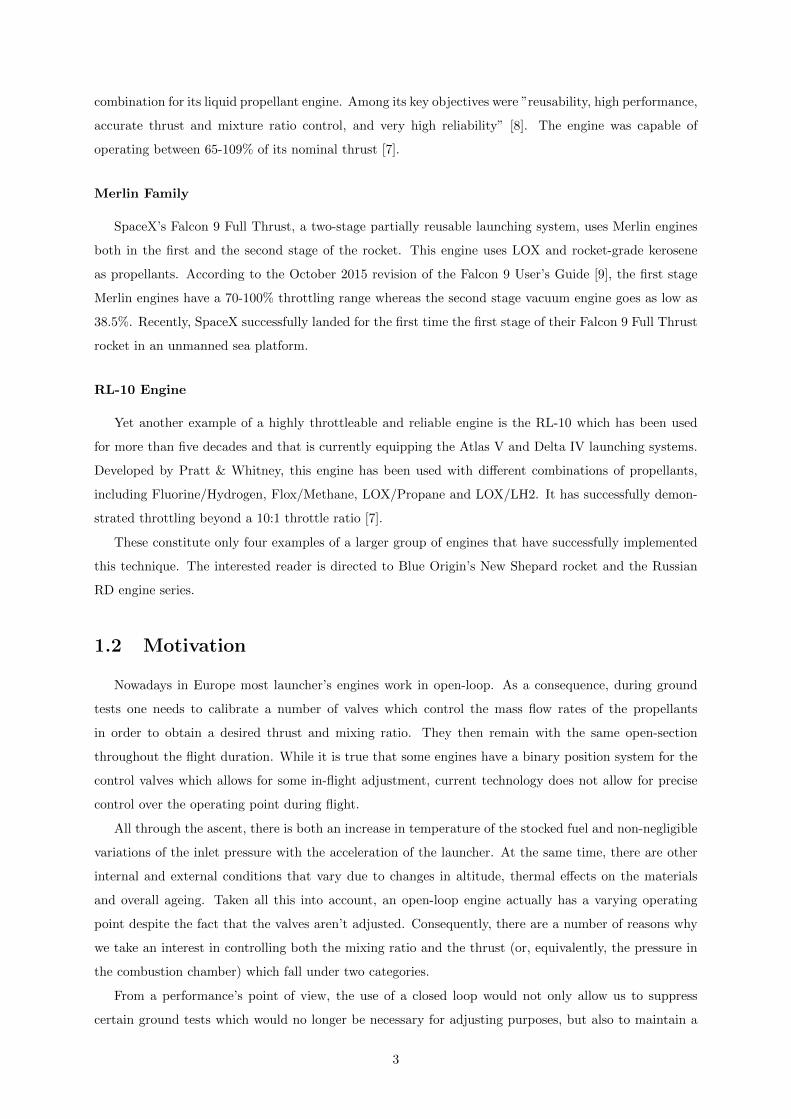
This relates to the fact that in order to guarantee launch success with a certain degree of probability, one

generally needs to compensate for the fact that either fuel, the oxidant or the reducer, may be the first

to run out as shown in figure 1.1. Evidently, the amount of extra fuel that is carried to ensure mission

success is directly linked with how precisely we can predict the consumption rate of both. Thus the great

interest in controlling the mixing ratio and the thrust in closed-loop.

Figure 1.1: Fuel consumption during flight.

Secondly, from a reusable launching system point of view, controlling these two quantities would

not only allow us to limit the mechanical and thermal stresses, which would be pivotal to preserve the

structure for subsequent launches, but also to take into account changing structural characteristics due

to ageing. In other words, the control system should be robust enough to parameter uncertainties to a

certain extent. Finally, softly landing the first stage of a launcher would undoubtedly require control over

a wide range of thrust capabilities.

These are the most important reasons why we seek to control the mixing ratio and the thrust of a

launcher’s engine. And while it is true that open-loop approaches can guarantee a certain level of thrust

and mixture ratio within a given tolerance with a limited number of firings of the actuators, a higher

degree of precision and thus of performance can be achieved in closed-loop.

Though the importance of making this technological jump is clear, current European rocket engines

have valves which are operated with pneumatic actuators, too inefficient to allow us to install a closed-

loop control of the engine. These run on Helium and are predictably costly to implement a real-time

control of the position of the valves. As a consequence, the electrification of these actuators is now under

study mainly to suppress or limit Helium consumption but also to allow for a closed-loop control of the

engine.

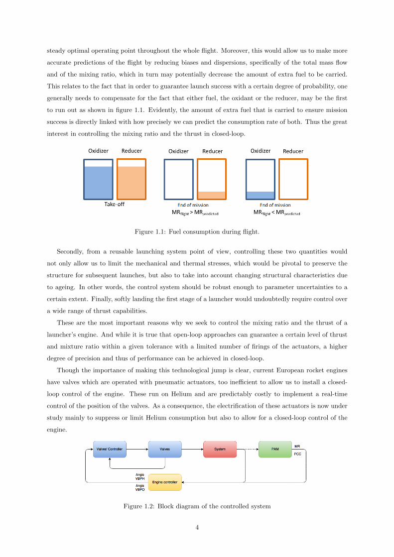
Figure 1.2: Block diagram of the controlled system

4

Figure 1.2 synthesizes the context of this thesis. In red there is the controlled system, namely the

engine and the fuel tanks. In blue, the valves, which they themselves have a feedback control loop in

order to precisely control their position. The inner-loop whose controller is in yellow is our main focus.

We receive a reference in both chamber pressure (PCC) and mixture ratio and the controller computes

a reference in angular position for both of the controlled valves. Finally, in green, the propellant active

management system (PAM) which will produce the reference of chamber pressure and mixing ratio with

the objective of balancing the consumption of both fuels so as to end the ascent with both fully consumed.

This system does not necessarily work in closed-loop, as highlighted in the diagram by the dotted line.

An open-loop approach, with an a priori knowledge of the relation between the valves’ position and the

mixing ratio, is also possible. This means that the PAM system doesn’t necessarily require the control

of the engine. Measuring the level of the fuels in the reservoirs and knowing before-hand, for each open-

section of the valves, the resulting mixing-ratio (although not with a high degree of precision), it can still

manage fuel consumption. Early studies indicate, however, that a closed-loop would allow for greater

optimization of the launcher’s performances.

1.3 Objectives

This thesis addresses several challenges concerning the control in closed-loop of thrust and mixture

ratio of a liquid-propellant rocket engine:

1. Modelling: obtaining a low order physical linear model of the engine constitutes one of the critical

aspects of this thesis; an analytic explicit form of a state-space model will be sought out.

2. Model analysis:

(a) Model validation over the operating domain;

(b) Determining the engine’s components responsible for the dominant modes;

(c) Analysing the effects of parameter uncertainties on the poles and zeros of the system;

(d) List the engine design parameters constraining the implementation of a control law;

3. Control law implementation: implementing and validating a robust control law capable of

maintaining with precision a desired equilibrium point and of transitioning towards a low-thrust

equilibrium point while respecting the established requirements;

Above all, the main goal is to establish a methodology easily applicable to different engines. As a

starting point, we use the European VINCI engine as a study-case.

1.4 Previous Work

LPRE’s with a varying thrust profile have been studied since the 1930’s. Prior to this period these

engines worked essentially at constant thrust. However, in the second half of this decade, German

5

researchers incorporated for the first time a manual throttling system in an LPRE that partially powered

a German Heinkel He 112 fighter aircraft. After this pioneer work, research was mainly focused on

”applicability to missile defense, weapons systems, and then space vehicles” [6].

However efficient the throttling technique is, there are other physical parameters that can be controlled

in order to obtain varying thrust. Several of these concepts were developed in the 1960’s and are described

in [7]. Varying the propellant flow rates is nonetheless the simplest way of controlling both mixture ratio

and thrust and it is the focus of this thesis.

This concept was demonstrated both in the LMDE and, later on, in the SSME. A renewed interest

in this technique arose recently with the prospect of enhancing performances of current launchers but

also with the objective of developing partially reusable launching systems. While recovering the first

stage of a satellite launcher may not be cost efficient, it allows companies to store multiple launchers and

readily respond to an eventual peak in demand which would otherwise be impossible to satisfy. There

are however limited references in the open literature on modelling and controller design for LPRE’s.

Simplified linear models around an equilibrium point are presented in [10] and [11]. These are not

very accurate mathematical models of the subsystems of an LPRE but their linear, time-invariant nature

is essential to apply known linear controller design techniques. In [12] the authors describe a model

identification technique for the SSME. Pseudorandom binary sequences are used as driving signals to

excite all modes of the system and a recursive maximum likelihood method algorithm is applied in order

to determine the transfer function coefficients for a linear model around an equilibrium point. Given that

the order of the system is unknown, parameters are estimated for models of increasing order until the

total estimation error converges to a minimum. In [13], the least squares technique is used to determine

a state-space formulation of the linearized system for the same engine.

The control of the mixture ratio and thrust of an LPRE is composed of two control loops, one for

each of the outputs. These control loops may be coupled or decoupled [14], and the control strategies

may rely on a linear or non-linear approaches.

In [15] the authors discuss the implementation of an integral and proportional-integral control strategy

for the Japanese LE-X cryogenic booster engine. In [11] a proportional-derivative-integral (PID) controller

is tested against a fuzzy logic controller in an academic simplified model of an LPRE constituted of 1st

order ordinary differential equations. Both are found to have acceptable performances although the PID

displays better performance.

In [14], a complete methodology based on ordinary describing function (DF) techniques for control

of an LPRE is presented. It discusses model identification around an operating point of interest which

should be previously characterized by the range of expected amplitudes and frequencies of excitation

signals. Moreover it highlights that DF techniques are able to handle discontinuities or multivalued

nonlinear terms whereas straight linearization fails in these cases. In [16] the same authors couple the

DF approach with factorization theory for controller design.

A non-linear state-space model linearization approach is described in [17]. After obtaining an 18 states

small signals model of the rocket engine, the Hankel model order reduction technique is applied to obtain

a 13 states reduced model. In this case, the authors seek to minimize damage to key subsystems of the

6

engine such as the turbines. Therefore, an H∞ approach is used to obtain a controller that minimizes

the energy between the perturbations and the regulated outputs as well as the oscillations during the

transient response. Moreover, a Life-Extending outer control loop is added which incorporates a non-

linear damage predicting model and a controller that minimizes the damage by employing a non-linear

programming technique known as Sequential Quadratic Programming. In [18] the same authors build on

this concept and present a more detailed account of this methodology.

1.5 Thesis Outline

Chapter 2 introduces the necessary propulsion fundamentals to understand the work principle of a

liquid-propellant rocket engine. Subsequently the main engine subsystems are introduced and briefly

described.

Chapter 3 briefly describes some elements of control theory that are required in the implementation

and analysis of the engine models as well as in the control of the VINCI engine. We start by formalizing

the linearization of a generic state-space model. The least-squares method for model identification is

then introduced, followed by a brief description of the matched DC gain reduction method. We proceed

to define the concepts of controllability and observability and wrap up the chapter addressing the use

of singular values to describe the behaviour of multiple-input multiple-output (MIMO) systems in the

frequency domain as well as a brief account of some considerations regarding robustness analysis.

Chapter 4 provides an overview of the VINCI engine characteristics, namely of its thermodynamic

cycle and of the available mechanisms to control the mixture ratio and the chamber pressure. It then

proceeds to present the analytic linear model of that same engine and its corresponding state-space

formulation.

Chapter 5 starts by addressing the implementation and analysis of the complete and reduced analytic

linear models. We then proceed to explain the need to obtain an identified linear model, both complete

and reduced, and validate the least-squares method as a model identification algorithm. A comparison is

drawn between the four analytic models and the reduced identified linear model is retained for controller

design. We finish the chapter by studying the effect of several design parameters over the dynamics of the

system. Conclusions are drawn regarding the dominant modes and the components that govern them.

Chapter 6 defines the control specifications to be met by the closed-loop system.

Chapter 7 describes the approach to design, implement and validate a modified PID controller. We

then characterize the obtained closed-loop in terms of closed-loop poles, modulus margin and frequency

response.

Chapter 8 concludes the present work by presenting the results of a simplified flight simulation on

the complete non-linear model of the VINCI engine as well as a robustness study against parametric

uncertainties and failure events.

7

8

Chapter 2

Liquid-propellant Engines

In this chapter the process through which one produces thrust is explained and some of the funda-

mental equations of rocketry are presented. The major subsystems of a liquid-propellant rocket engine

are briefly described and their importance to the overall engine architecture is outlined.

The propulsion fundamentals are explained extensively in [2] and [19], over which this chapter is

largely based on. Engine design and its major subsystems are described in detail in [19].

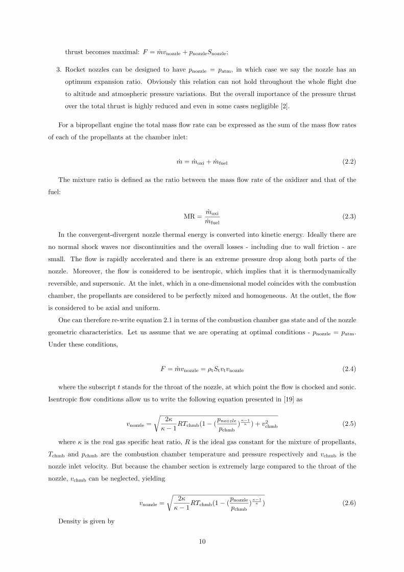
2.1 Propulsion Fundamentals

The principal function of a chemical rocket propulsion system is to generate a propulsive force - thrust

- by converting chemical energy stored in the propellants into kinetic energy of the gaseous combustion

products with maximum efficiency. The first step of this conversion occurs in the combustion chamber

where the chemical energy is converted into thermal energy with an associated efficiency - ηcomb. The

resulting high temperature, high pressure gases tend to expand and be ejected at high speeds through

the nozzle - thermal energy is converted into kinetic energy with an efficiency coefficient ηexp . According

to the third law of motion, the momentum conservation imparts a force in the rocket which is formalized

in equation 2.1.

F = mvnozzle + (pnozzle − patm)Snozzle (2.1)

where m is the total mass flow exiting the nozzle, vnozzle is the matter ejection velocity relative to

the vehicle, pnozzle is the pressure of the gases at the exit of the nozzle, patm is the atmospheric pressure

and Snozzle is the section of the nozzle outlet. The first term is the momentum thrust whereas the second

term is commonly called the pressure thrust. The latter arises from the exerted force by the surrounding

fluid in which the rocket is immersed. There are three important considerations to make at this point:

1. Since the atmospheric pressure is a decreasing function of altitude, thrust will increase during the

ascent. Typical values point to a 10-30% overall thrust change due to altitude variations [2];

2. In vacuum, or at sufficiently high altitudes, atmospheric pressure is considered to be negligible and

9

thrust becomes maximal: F = mvnozzle + pnozzleSnozzle;

3. Rocket nozzles can be designed to have pnozzle = patm, in which case we say the nozzle has an

optimum expansion ratio. Obviously this relation can not hold throughout the whole flight due

to altitude and atmospheric pressure variations. But the overall importance of the pressure thrust

over the total thrust is highly reduced and even in some cases negligible [2].

For a bipropellant engine the total mass flow rate can be expressed as the sum of the mass flow rates

of each of the propellants at the chamber inlet:

m = moxi + mfuel (2.2)

The mixture ratio is defined as the ratio between the mass flow rate of the oxidizer and that of the

fuel:

MR =moxi

mfuel(2.3)

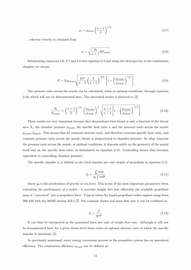
In the convergent-divergent nozzle thermal energy is converted into kinetic energy. Ideally there are

no normal shock waves nor discontinuities and the overall losses - including due to wall friction - are

small. The flow is rapidly accelerated and there is an extreme pressure drop along both parts of the

nozzle. Moreover, the flow is considered to be isentropic, which implies that it is thermodynamically

reversible, and supersonic. At the inlet, which in a one-dimensional model coincides with the combustion

chamber, the propellants are considered to be perfectly mixed and homogeneous. At the outlet, the flow

is considered to be axial and uniform.

One can therefore re-write equation 2.1 in terms of the combustion chamber gas state and of the nozzle

geometric characteristics. Let us assume that we are operating at optimal conditions - pnozzle = patm.

Under these conditions,

F = mvnozzle = ρtStvtvnozzle (2.4)

where the subscript t stands for the throat of the nozzle, at which point the flow is chocked and sonic.

Isentropic flow conditions allow us to write the following equation presented in [19] as

vnozzle =

√2κ

κ− 1RTchmb(1− (

pnozzlepchmb

)κ−1κ ) + v2

chmb (2.5)

where κ is the real gas specific heat ratio, R is the ideal gas constant for the mixture of propellants,

Tchmb and pchmb are the combustion chamber temperature and pressure respectively and vchmb is the

nozzle inlet velocity. But because the chamber section is extremely large compared to the throat of the

nozzle, vchmb can be neglected, yielding

vnozzle =

√2κ

κ− 1RTchmb(1− (

pnozzle

pchmb)κ−1κ ) (2.6)

Density is given by

10

ρt = ρchmb

(κ+ 1

2

) 11−κ

(2.7)

, whereas velocity is obtained from

vt =

√2κ

κ+ 1RTchmb (2.8)

Substituting equations 2.6, 2.7 and 2.8 into equation 2.4 and using the ideal gas law in the combustion

chamber we obtain:

F = Stpchmb

√√√√ 2κ2

κ− 1

(2

κ+ 1

) κ+1κ−1

[1−

(pnozzle

pchmb

)κ−1κ

](2.9)

The pressure ratio across the nozzle can be calculated, when at optimal conditions, through equation

2.10, which will not be demonstrated here. The interested reader is directed to [2].

StSnozzle

=

(κ+ 1

2

) 1κ−1

(pnozzle

pchmb

) 1κ

√√√√κ+ 1

κ− 1

[1−

(pnozzle

pchmb

)κ−1κ

](2.10)

These results are very important because they demonstrate that thrust is only a function of the throat

area St, the chamber pressure pchmb, the specific heat ratio κ and the pressure ratio across the nozzle

pnozzle/pchmb. This means that for constant mixture ratio, and therefore constant specific heat ratio, and

constant pressure ratio across the nozzle, thrust is proportional to chamber pressure. In what concerns

the pressure ratio across the nozzle, at optimal conditions, it depends solely on the geometry of the nozzle

itself and on the specific heat ratio, as formulated on equation 2.10. Controlling thrust thus becomes

equivalent to controlling chamber pressure.

The specific impulse Is is defined as the total impulse per unit weight of propellant in equation 2.11.

Is =

∫ t0Fdt

g0

∫mdt

(2.11)

where g0 is the acceleration of gravity at sea level. This is one of the most important parameters when

evaluating the performance of a rocket - it provides insight into how efficiently the available propellant

mass is ”converted” into a propulsive force. Typical values for liquid-propellant rocket engines range from

300-450 with the SSME having 453.5 [7]. For constant thrust and mass flow rate it can be redefined as

Is =F

g0m(2.12)

It can thus be interpreted as the generated force per unit of weight flow rate. Although it will not

be demonstrated here, for a given thrust level there exists an optimal mixture ratio at which the specific

impulse is maximum [2].

As previously mentioned, every energy conversion process in the propulsive system has an associated

efficiency. The combustion efficiency ηcomb can be defined as:

11

ηcomb =Pthermal

Pchem=Pthermal

mQR(2.13)

where Pthermal is the available thermal power, Pchem is the available chemical power and QR is the

energy available per unit mass of chemical propellant. This efficiency is generally high, approximately

94-99% [2].

The conversion from thermal to kinetic energy also has an associated efficiency defined as:

ηexp =Pkin

Pthermal=

12mv

2nozzle

ηcombPchem(2.14)

where Pkin is the available kinetic power. This efficiency is generally under 40%.

2.2 Engine Work Principle and Classification

As mentioned in the previous section, the purpose of an LPRE is to convert chemical energy into

kinetic energy, or equivalently into propulsive power, with maximum efficiency. Six major subsystems

take part in this conversion process and form the engine as a whole. Their description below is based on

[19]. The first four subsystems are represented in figure 2.1.

1. Thrust-chamber assembly;

2. Propellant feed system;

3. Turbine-drive system;

4. Propellant control system;

5. Electric and pneumatic controller systems;

6. Thrust-vector control system (TVC);

Thrust-chamber Assembly

The thrust-chamber assembly is probably the most critical subsystem in terms of performance. The

combustion chamber receives at its inlet high pressure propellants provided by the propellant feed system.

Within it, mixture, ignition and basically the whole combustion process takes place. The combustion

products are then expelled at high temperatures and speeds through a convergent-divergent nozzle.

While the combustion chamber is responsible for converting chemical energy into thermal energy, the

nozzle is equally important in converting the enthalpy of the combustion gases into kinetic energy. In

nominal conditions, the gases are accelerated to sonic speeds at the throat of the nozzle, the minimal

section point, and then further accelerated by the divergent section to supersonic speeds. However, for a

particular design, there is only one value of ambient pressure for which an ideal expansion occurs. That

is to say that for chocked flow at the throat of the nozzle, where Mach number equals 1, if the ambient

pressure does not match the exit pressure for those particular flow conditions, a pressure recovery must

12

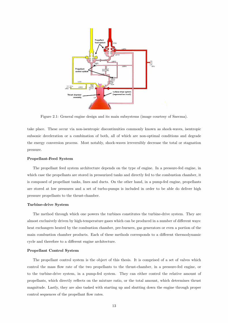
Figure 2.1: General engine design and its main subsystems (image courtesy of Snecma).

take place. These occur via non-isentropic discontinuities commonly known as shock-waves, isentropic

subsonic deceleration or a combination of both, all of which are non-optimal conditions and degrade

the energy conversion process. Most notably, shock-waves irreversibly decrease the total or stagnation

pressure.

Propellant-Feed System

The propellant feed system architecture depends on the type of engine. In a pressure-fed engine, in

which case the propellants are stored in pressurized tanks and directly fed to the combustion chamber, it

is composed of propellant tanks, lines and ducts. On the other hand, in a pump-fed engine, propellants

are stored at low pressures and a set of turbo-pumps is included in order to be able do deliver high

pressure propellants to the thrust-chamber.

Turbine-drive System

The method through which one powers the turbines constitutes the turbine-drive system. They are

almost exclusively driven by high-temperature gases which can be produced in a number of different ways:

heat exchangers heated by the combustion chamber, pre-burners, gas generators or even a portion of the

main combustion chamber products. Each of these methods corresponds to a different thermodynamic

cycle and therefore to a different engine architecture.

Propellant Control System

The propellant control system is the object of this thesis. It is comprised of a set of valves which

control the mass flow rate of the two propellants to the thrust-chamber, in a pressure-fed engine, or

to the turbine-drive system, in a pump-fed system. They can either control the relative amount of

propellants, which directly reflects on the mixture ratio, or the total amount, which determines thrust

magnitude. Lastly, they are also tasked with starting up and shutting down the engine through proper

control sequences of the propellant flow rates.

13

As explained in section 1.2, vehicle performance, namely safe engine operation and minimum propel-

lant outage, is maximized when working at a specific thrust level and mixture ratio. At a steady state

regime, these two parameters can either be controlled in open or closed-loop depending on the desired

accuracy.

Electric and Pneumatic Controller Systems

The above-mentioned valves are either electrically or pneumatically controlled. Pneumatic controllers

use Helium, also used for tank pressurization, to power the actuators. This solution is reliable and cost-

effective for sporadic stepwise valve adjustment in an open-loop look-up table control approach. However,

if one is interested in a closed loop active continuous control throughout the whole flight duration, electric

controller systems are more cost effective.

TVC

The thrust-vector control system tilts the engine in order to provide directional control. It is used in

the guidance control system.

2.2.1 Liquid Propellants

The propellant is the source of energy of the engine. Its choice is of major importance in the design

for it affects overall performance, total cost and structure architecture. Some other aspects to take into

account when selecting the propellant include price, supply, storage conditions, pollution, health, and

safety.

According to the type and number of used liquid propellants, there are multiple classifications. Firstly,

an engine may run on a single propellant - mono-propellant - which is often a mixture of an oxidizer and

a fuel. These engines are simpler, particularly the propellant feed system and the turbine drive system,

but also under-perform when compared to a bi-propellant engine. These employ an oxidizer and a fuel

which are stored separately, for instance oxygen and hydrogen. If their mixture ignites spontaneously

then the combination is called hypergolic. Otherwise the thrust-chamber must possess an ignition system

to set off the combustion. This thesis focuses solely on bi-propellant engines such as the VINCI engine.

Moreover if a propellant can be stored at ambient temperature and pressure it is called earth-storable.

These are simpler to handle for obvious reasons. In contrast, cryogenic propellants are liquefied gases

which have very low boiling points and therefore require special storage conditions. The most common

example is LOX and LH2.

14

2.3 Summary

In this chapter important expressions to calculate thrust were presented. Mixture-ratio, our second

quantity of interest, was defined. The equivalence between thrust and chamber pressure at constant

mixture ratio and at optimal conditions was demonstrated. The work principle of a liquid-propellant

rocket engine, along with a brief description of its major subsystems, was then presented. A classification

system in function of the liquid propellants’ characteristics and of the propellant-feed system was also

discussed.

15

16

Chapter 3

Elements of Control Theory

In this chapter several elements of control theory are addressed.They are particularly useful to un-

derstand the determination and analysis of a low order physical linear model of the VINCI engine. We

start by formalizing the linearization theory of non-linear state-space models about an equilibrium point.

Afterwards we introduce the least-squares method for linear state-space models identification [20]. We

then proceed to formalize the matched DC gain method for model reduction, one of the known few which

allows us to keep a model with physical meaning. The controllability and observability concepts and

matrices are then introduced [21]. A definition of the singular value decomposition, its properties and

how it can be used to determine the modulus margin and therefore characterize stability and robustness

of MIMO systems is presented [21]. Lastly a brief account of model uncertainty sources is provided [21].

3.1 State-space Model Linearization

A system is said to be in state variable form if its dynamic model is described by n first order

differential equations and p algebraic equations of the form

x1 = f1(x1, ..., xn, u1, ..., um)

x2 = f2(x1, ..., xn, u1, ..., um)...

xn = fn(x1, ..., xn, u1, ..., um)

y1 = g1(x1, ..., xn, u1, ..., um)...

yp = gp(x1, ..., xn, u1, ..., um)

(3.1)

, where x = [x1, ..., xn]T is the state vector, u = [u1, ..., um] the control input and [y1, ..., yp] the control

output. Functions f = [f1, ..., fn]T and g = [g1, ..., gp]T are generally non-linear, as is the case of the

VINCI engine. However, in order to be able to apply known linear control techniques, one can generally

describe the behaviour of a non-linear system in the vicinity of a system configuration called equilibrium

point with a linear model given by

17

x = Ax+Bu

y = Cx+Du(3.2)

Matrix A has dimensions n× n, B is n×m, C is p× n and D is p×m.

Definition 3.1.1. Equilibrium point Let us consider a system in the state-space form 3.1 and a constant

input u. Then if f(x, u) = 0, x is said to be an equilibrium point of the system.

The state-space form can be approximated by a first-order Taylor expansion around any equilibrium

point, yielding the linear model

∆x = A∆x+B∆u

∆y = C∆x+D∆u(3.3)

, where ∆x denotes x− x, ∆u denotes u− u and ∆y denotes y− y. Matrices A,B,C,D are expressed

as:

A =

[∂f

∂x

]x,u

=

∂f1∂x1

(x, u) . . . ∂f1∂xn

(x, u)...

. . ....

∂fn∂x1

(x, u) . . . ∂fn∂xn

(x, u)

B =

[∂f

∂u

]x,u

=

∂f1∂u1

(x, u) . . . ∂f1∂un

(x, u)...

. . ....

∂fn∂u1

(x, u) . . . ∂fn∂un

(x, u)

C =

[∂g

∂x

]x,u

D =

[∂g

∂u

]x,u

It is worth mentioning that, for a particular application, the linearization is only valid in a sufficiently

small domain around the equilibrium point, the extent of which may be difficult to estimate. A possible

approach would be to determine the second-order term of the Taylor expansion which, for high-order

systems, may become impractical.

3.2 Model Identification

System identification methods are a class of techniques which allow us to build mathematical models

of dynamic systems using measured data. These techniques may either rely on known dynamic laws of

the system or solely on input-output behaviour without any knowledge of the dynamic states or of the

governing equations of the system. Their application can also either be in the time-domain or in the

frequency-domain.

18

In this section we will introduce and formalize the least-squares method for model identification. This

method, alongside the analytic approach, will take part in our quest for a low-order physical linear model

of the VINCI engine.

3.2.1 Least-squares Method

Often in the world of physics we expect to find linear relationships between variables. Seldom, however,

are these relations perfectly linear due to experimental errors and, frequently, to approximately linear

phenomenons. Nonetheless, in order to simplify our models, we look to establish ”the best” linear fit

to the observed data. The least-squares method defines and quantifies what the best fit is and offers a

solution to this common problem [22].

Let us consider the example of a discrete state-space linear model:

xk+1 = Axk +Buk

yk = Cxk +Duk(3.4)

This model can be rearranged in the following form:

[xTk+1 yTk

]=[xTk uTk

] AT CT

BT DT

If written for k = 1, ...N , then we obtain

Y = ΘM ⇔

xT2 yT1...

...

xTN+1 yTN

=

xT1 uT1...

...

xTN uTN

AT CT

BT DT

, which for N greater than the number of states of the system becomes an overdetermined system.

The least-squares approach consists of finding the solution which minimizes the error function

E =‖ ΘM − Y ‖2 (3.5)

Calculating the gradient of this function and imposing ∂E∂M = 0 to obtain the minima

M = (ΘTΘ)−1ΘTY (3.6)

,which corresponds to the pseudo-inverse of matrix Θ multiplied by Y .

This method is often inadequate for model identification because it requires knowing both the order

and the states of the system. Contrarily, when this is known, it has the advantage of yielding a model

with the desired state-space base.

It is worth noting that, in the case of a linear state-space model, the least-squares solution error

asymptotically decreases with the sampling frequency. In order to completely capture the system’s

dynamics this frequency must respect Shannon’s theorem which states that the sampling frequency must

be at least twice as large as the natural frequency of the fastest mode.

19

3.3 Reduction Methods

With today’s need to model ever-increasingly complex physical phenomena in order to properly simu-

late a system’s behaviour, mathematical models have grown to be highly detailed. However, we often do

not need to model every single detail to capture the essentials of a system’s dynamics. This is particularly

true in linear control theory. More often than not, highly complex phenomena can be described by a

handful of dominant modes which are sufficient for control law design [23]. In fact, most of the available

techniques today require low-order models to be applicable in practice.

The process of obtaining a low-order model from a high-order complete model is commonly called

model order reduction. The following section focuses on a technique which uses physical insight to remove

model states while preserving input-output behaviour, particularly at low frequencies.

3.3.1 Matched DC Gain Method

Let us consider the classical linear time-invariant state-space model formulation:

x = Ax+Bu

y = Cx+Du(3.7)

The state-vector x can be decomposed as x = [xnr, xr]T , where xnr constitutes the set of states to be

kept and xr the set of states to be eliminated. The state-space model thus becomes:

˙ xnr

xr

=

A11 A12

A21 A22

xnr

xr

+

B1

B2

u

y =

C11 C12

C21 C22

xnr

xr

+

D1

D2

u(3.8)

Assuming the dynamics of xr to be infinitely fast, then xr ≈ 0 and the model can be rewritten as:

xnr = (A11 −A12A−122 A21)xnr + (B1 −A12A

−122 B2)u

y =

(C11 − C12A−122 A21)

(C21 − C22A−122 A21)

xnr +

(D1 − C12A−122 B2)

(D2 − C22A−122 B2)

u (3.9)

The matched DC-gain method preserves the static gain of the original model. Therefore, it conserves

the model’s behaviour at low frequencies. When compared to other more sophisticated methods, it has

the advantage of conserving the state-space base, in other words, the reduced model can be interpreted

physically if the full model has an explicit physical-related state-vector. This is of first importance to

our objectives because it will allow us to determine which elements and physical parameters within the

engine play a significant role in the system’s dominant dynamics. One of its main disadvantages concerns

the choice of the set of states to be eliminated. That analysis has to be made on a model to model basis

and often relies on physical insight of the dynamics of the system.

20

3.4 Controllability and Observability

Controllability is associated with the question of whether an input exists such that our system can

reach any given final state x1 departing from a generic initial state x0 in a bounded time interval.

Observability, on the other hand, determines whether one can deduce the system’s full state vector x

from the system’s measurements y and inputs u, also over a bounded time interval.

Definition 3.4.1. Controllability Let us consider a system in a state-space form x = Ax + Bu, x(t =

0) = x0. The state x0 is said to be controllable if for any given final state x1 there exists an input u[0,t1]

and time t1 > 0 such that the system’s state is steered to x(t1) = x1. If every x0 state is controllable,

the (A,B) pair is said to be completely controllable.

Definition 3.4.2. Observability Let us consider a system in a state-space form x = Ax + Bu, y = Cx,

x(t = 0) = x0. The initial state x0 is said to be observable if there exists a time t1 > 0 such that we are

able to determine x0 solely through the measurements y[0,t1] and the inputs u[0,t1] . If every x0 state is

observable, the (A,C) pair is said to be completely observable.

While controllability and observability can be quantified, for the purposes of this thesis we will solely

focus on a binary criteria for these two properties.

3.4.1 Controllability and Observability Matrices

Let us consider the linear time-invariant system in equation 3.10 and its solution in equation 3.11.

x(t) = Ax(t) +Bu(t) (3.10)

x(t) = eA(t−t0)x(t0) +

∫ t

t0

eA(t−τ)Bu(τ)dτ (3.11)

The reachable state vectors in the time interval [t0, t1] depend exclusively of the reachability map,

defined as:

L[t0,t1](u(t)) =

∫ t1

t0

eA(t1−τ)Bu(τ)dτ (3.12)

The pair (A,B) is thus said to be controllable if and only if the map is surjective (onto), in other

words if we can find u(t) such that x(t1) = x1. The Cayley-Hamilton theorem, by providing us with a

relationship between the n-th and higher powers of A and the (n-1)-th and lower powers of A, enables us

to write:

e−Aτ =

n−1∑i=0

αi(τ)Ai (3.13)

where αi are scalar time functions and n is the order of the system. By substitution onto equation

3.11 and simplification we obtain:

21

e−At1x1 − e−At0x0 =∑n−1i=0 (AiB)

∫ t1t0αi(τ)u(τ)dτ

=[B,AB,A2B, . . . , An−1B

]

∫ t1t0α0(τ)u(τ)dτ

...∫ t1t0αn−1(τ)u(τ)dτ

(3.14)

thus demonstrating that we can indeed find u(t) such that the equation is verified if and only if[B,AB,A2B, . . . , An−1B

]is invertible or, equivalently, if the controllability matrix has full row rank.

Let us consider an input-free system for the sake of conciseness whilst studying observability. In the

general case, the reasoning remains identical although the system’s input is then required in order to

determine the initial state of the system.

y(t0) = Cx(t0)

˙y(t0) = Cx(t0) = CAx(t0)...

yn−1(t0) = Cxn−1(t0) = CAn−1x(t0)

which can be rearranged in matrix form:

y(t0)

y(t0)...

yn−1(t0)

=

C

CA...

CAn−1

x(t0) (3.15)

Thus it can be concluded that the initial state of the system may be determined from its measurements

(and inputs should we consider the system’s input) in a finite time interval if and only if the observability

matrix[C;CA; . . . ;CAn−1

]is invertible or, equivalently, if it has full row rank. Moreover, adding higher-

derivatives does not increase the observability because the Cayley-Hamilton theorem guarantees that

higher than (n−1) powers of A can always be expressed in function of the first (n−1) powers. Therefore

these extra equations would be linearly dependent on the previously written ones.

3.5 Singular Values and Modulus Margin

The frequency response analysis is a very powerful tool to characterize the stability, performance

and robustness of a system. Several techniques and rules have been well established for the analysis of

single-input single-output (SISO) systems, namely the definition of gain and phase margins which can,

for example, be deduced from the Bode plot of the transfer function. These two concepts account for

the robustness of the system to uncertainty, perturbations or unmodeled dynamics. While the transfer

function frequency response can be directly generalized to MIMO systems by considering all different

transfer functions from each input to each output, the gain and phase margin concepts can not.

Let us consider the gain at a given frequency:

22

||y(ω)||2||u(ω)||2

=||G(jω)u(ω)||2||u(ω)||2

=

√y2

11 + y212 + ...√

u211 + u2

12 + ...(3.16)

Because the input and output are now vectors, we are obliged to introduce a norm. Moreover, the

gain, which in SISO systems depends solely on frequency, is now also a function of the direction of the

input but still independent of its magnitude. The introduction of the singular value decomposition (SVD),

rigorously defined below, allows us to extract useful information about the gain of the system despite the

introduction of the direction dependency.

Definition 3.5.1. Unitary matrix A complex matrix U is said to be unitary if and only if UH = U−1.

All of its eigenvalues and singular values have an absolute value equal to 1.

Consider an m× n transfer matrix G(jω) at a given frequency and its singular value decomposition:

G = UΣV H (3.17)

where Σ is an m × n matrix with k = min(m,n) real, non-negative singular values, σi, arranged in

descending order along its main diagonal; U is an m ×m unitary matrix of output singular vectors, ui,

forming an orthonormal bases for the output space; V is an n×n unitary matrix of input singular vectors,

vi, forming an orthonormal bases for the input space.

The input and output directions, ui and vi, are related through the singular values. Since V is unitary

then V HV = I and we can thus write:

Gvi = σiui (3.18)

which means that if we consider an input in the direction vi, we obtain an output in the direction ui

and, given that both vectors have a unitary norm, σi directly represents the gain of the system in this

particular direction. Most notably, it can be shown that for a given frequency, the maximum gain for

any input direction corresponds to the maximum singular value:

maxu6=0

||Gu||2||u||2

= σ(G(jω)) (3.19)

Inversely, the smallest gain for any input direction is equal to the minimum singular value:

minu6=0

||Gu||2||u||2

=¯σ(G(jω)) (3.20)

The modulus margin, the only one that can be generalized to MIMO systems, is defined as the smallest

distance from the open-loop frequency-domain response L(jω) = G(jω)K(jω) to the critical point and

can be measured by the radius r of the circle centered on the critical point and tangent to the L(jω)

response:

r = minω|1 +G(jω)K(jω)| (3.21)

23

which for MIMO systems can be reformulated as:

r = minω ¯σ(I +G(jω)K(jω)) (3.22)

Let us consider the inverse of a non-singular square matrix A:

A−1 = V Σ−1UH (3.23)

We immediately obtain the SVD of A−1 with the singular values arranged in ascending order. One

can therefore conclude that:

σ(A−1) =1

¯σ(A)

(3.24)

Thus enabling us to rewrite equation 3.22

r = minω

1σ(I+G(jω)K(jω))−1

1r = max

ωσ(I +G(jω)K(jω))−1 = ||S(s)||∞

(3.25)

,S(s) being the output sensitivity transfer function and || · ||∞ the H-infinity norm, defined, for stable

systems, to be the maximum gain among all frequencies and input directions - and therefore the maximum

of the maximum singular value for MIMO systems.

It is important to highlight that the determination of the modulus margin, as well as the use of other

analysis tools, requires the correct scaling of the system so as to have output errors with comparable

magnitudes. A proper way to do so involves dividing each variable by its maximum expected or allowed

value, which makes them less than one in magnitude.

u = Usclu =

umax

1 . . . 0...

. . ....

0 . . . umaxl

u1

...

ul

(3.26)

where u is the scaled variable, Uscl is a diagonal scaling matrix, u is the original vector and l its length.

When scaling the inputs and outputs of a state-space representation one obtains:

x = Ax+BUsclu

y = Y −1scl Cx+ Y −1

0 DUsclu(3.27)

3.6 Robustness Analysis

Control laws are often based on a single dynamic model of the system, e.g the nominal plant model. In

reality, it is inevitable, however, that there is a mismatch between the theoretical model upon which our

control law was based and the actual system. Consequently, it is a fundamental step of controller design

to ensure that stability and performance are insensitive to these uncertainties. Hereafter we present an

extensive list of uncertainty sources:

24

1. Non-linearities are often not taken into account in the control design method and may therefore have

an important impact on stability and performance of the closed-loop system; Common examples

include saturations, backlash and time delays.

2. Unmodelled dynamics, particularly at high frequencies due to numerical limitations of the identifi-

cation methods, or even caused by simplification of the dynamic equations modelling the system.

3. Uncertainty over parameters describing the system, whether because they evolve during operation,

because a precise measurement is impractical or simply because the fabrication of two components

of the same kind never yields the same exact result.

4. Changing operating conditions, particularly when the controller design process is based on the

linearization of the system around an equilibrium point.

5. Failure events during operation may cause drastic and sudden parameter variation.

The key idea is to guarantee that despite the whole set of uncertainties, even in the worst-case scenario,

stability and performance of the closed-loop are still guaranteed. Several approaches to resolve this

problem are available, featuring in particular the µ analysis developed in the H∞ framework. Nonetheless,

due to the number of uncertain parameters and the complexity of our system, this strategy was found

to be inadequate. Moreover, because the system is naturally stable, this complex and heavy method is

expected to add little value to the analysis.

We will thus focus on the multi-model approach in order to handle parametric uncertainties which

are the greatest source of uncertainty of the VINCI engine model. A finite set of perturbed linear models

- the uncertainty set - will be generated according to criteria to be defined in chapter 8. Stability and

performance will be evaluated over this set. The main disadvantage of this approach is that it gives us

no indication on how to generate the uncertainty set nor does it guarantee us to cover the worst-case.

On the other hand, it facilitates handling a high number of independent parameter uncertainties.

3.7 Summary

In this chapter important methods and concepts to the remainder of this thesis were introduced.

Firstly, a state-space model linearization technique was introduced. The least-squares method was for-

malized as an identification method to obtain a discrete state-space model of a system. A reduction

method which preserves the state-space base and the low frequency behaviour of the system was pre-

sented. The concepts of controllability and observability were introduced. Then the SVD was formalized

and its practical application for determining the modulus margin was presented. Lastly we focused on

sources of model uncertainty and we gave a very brief overview of possible methods to analyse a system’s

robustness.

25

26

Chapter 4

VINCI Engine

In this chapter an in-depth explanation of the thermodynamic cycle of the VINCI engine will be

provided, followed by an overview of the available actuators to perform the closed-loop control and

culminating with the presentation and linearisation of the governing equations of the engine. Lastly the

equations are assembled to form a linear state-space model about an equilibrium point.

4.1 Introduction

The VINCI engine is expected to power the upper stage of the Ariane 6 launcher. Developed by

Snecma, it is a liquid-bipropellant pump-fed engine which uses LOX as an oxidizer and LH2 as a fuel,

both of which are cryogenic propellants. Its characteristics at nominal level are presented in table 4.1

[24].

The VINCI engine constitutes the first numerical application of the methodology to be developed

in this thesis. As described in section 1.3, among our objectives are the development of a linear model

enabling us to study the dominant dynamic modes of the system as well as the implementation of a

closed-loop controller of thrust and mixture ratio.

The most detailed in-house model of this engine was built using CARINS (unsteady network cal-

culator), a code developed by CNES (Centre National d’Etudes Spatiales)for rocket engine transient

modelling. Much like Simulink, this software allows us to describe a system with an assemble of blocks

or subsystems, each of which represents a component of the actual engine - for instance a turbine, a

pump or a cavity. There are, however, some specific rules to be applied when using CARINS. The system

must be causal and the governing equations must be explicit. This often induces the use of intermediate

parameters or fictional elements which do not arise from physical modelling but rather as a craftiness to

overcome the software’s limitations. Nonetheless, these will be discarded for our model is not constrained

by such limitations and will be purely a description of the physical laws that govern the elements of the

engine.

27

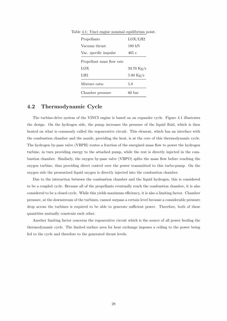
Table 4.1: Vinci engine nominal equilibrium point.

Propellants LOX/LH2

Vacuum thrust 180 kN

Vac. specific impulse 465 s

Propellant mass flow rate

LOX

LH2

33.70 Kg/s

5.80 Kg/s

Mixture ratio 5.8

Chamber pressure 60 bar

4.2 Thermodynamic Cycle

The turbine-drive system of the VINCI engine is based on an expander cycle. Figure 4.1 illustrates

the design. On the hydrogen side, the pump increases the pressure of the liquid fluid, which is then

heated on what is commonly called the regenerative circuit. This element, which has an interface with

the combustion chamber and the nozzle, providing the heat, is at the core of this thermodynamic cycle.

The hydrogen by-pass valve (VBPH) routes a fraction of the energized mass flow to power the hydrogen

turbine, in turn providing energy to the attached pump, while the rest is directly injected in the com-

bustion chamber. Similarly, the oxygen by-pass valve (VBPO) splits the mass flow before reaching the

oxygen turbine, thus providing direct control over the power transmitted to this turbo-pump. On the

oxygen side the pressurized liquid oxygen is directly injected into the combustion chamber.

Due to the interaction between the combustion chamber and the liquid hydrogen, this is considered

to be a coupled cycle. Because all of the propellants eventually reach the combustion chamber, it is also

considered to be a closed cycle. While this yields maximum efficiency, it is also a limiting factor. Chamber

pressure, at the downstream of the turbines, cannot surpass a certain level because a considerable pressure

drop across the turbines is required to be able to generate sufficient power. Therefore, both of these

quantities mutually constrain each other.

Another limiting factor concerns the regenerative circuit which is the source of all power feeding the

thermodynamic cycle. The limited surface area for heat exchange imposes a ceiling to the power being

fed to the cycle and therefore to the generated thrust levels.

28

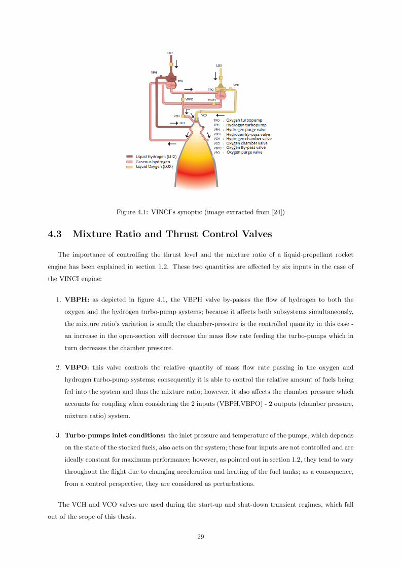
Figure 4.1: VINCI’s synoptic (image extracted from [24])

4.3 Mixture Ratio and Thrust Control Valves

The importance of controlling the thrust level and the mixture ratio of a liquid-propellant rocket

engine has been explained in section 1.2. These two quantities are affected by six inputs in the case of

the VINCI engine:

1. VBPH: as depicted in figure 4.1, the VBPH valve by-passes the flow of hydrogen to both the

oxygen and the hydrogen turbo-pump systems; because it affects both subsystems simultaneously,

the mixture ratio’s variation is small; the chamber-pressure is the controlled quantity in this case -

an increase in the open-section will decrease the mass flow rate feeding the turbo-pumps which in

turn decreases the chamber pressure.

2. VBPO: this valve controls the relative quantity of mass flow rate passing in the oxygen and

hydrogen turbo-pump systems; consequently it is able to control the relative amount of fuels being

fed into the system and thus the mixture ratio; however, it also affects the chamber pressure which

accounts for coupling when considering the 2 inputs (VBPH,VBPO) - 2 outputs (chamber pressure,

mixture ratio) system.

3. Turbo-pumps inlet conditions: the inlet pressure and temperature of the pumps, which depends

on the state of the stocked fuels, also acts on the system; these four inputs are not controlled and are

ideally constant for maximum performance; however, as pointed out in section 1.2, they tend to vary

throughout the flight due to changing acceleration and heating of the fuel tanks; as a consequence,

from a control perspective, they are considered as perturbations.

The VCH and VCO valves are used during the start-up and shut-down transient regimes, which fall

out of the scope of this thesis.

29

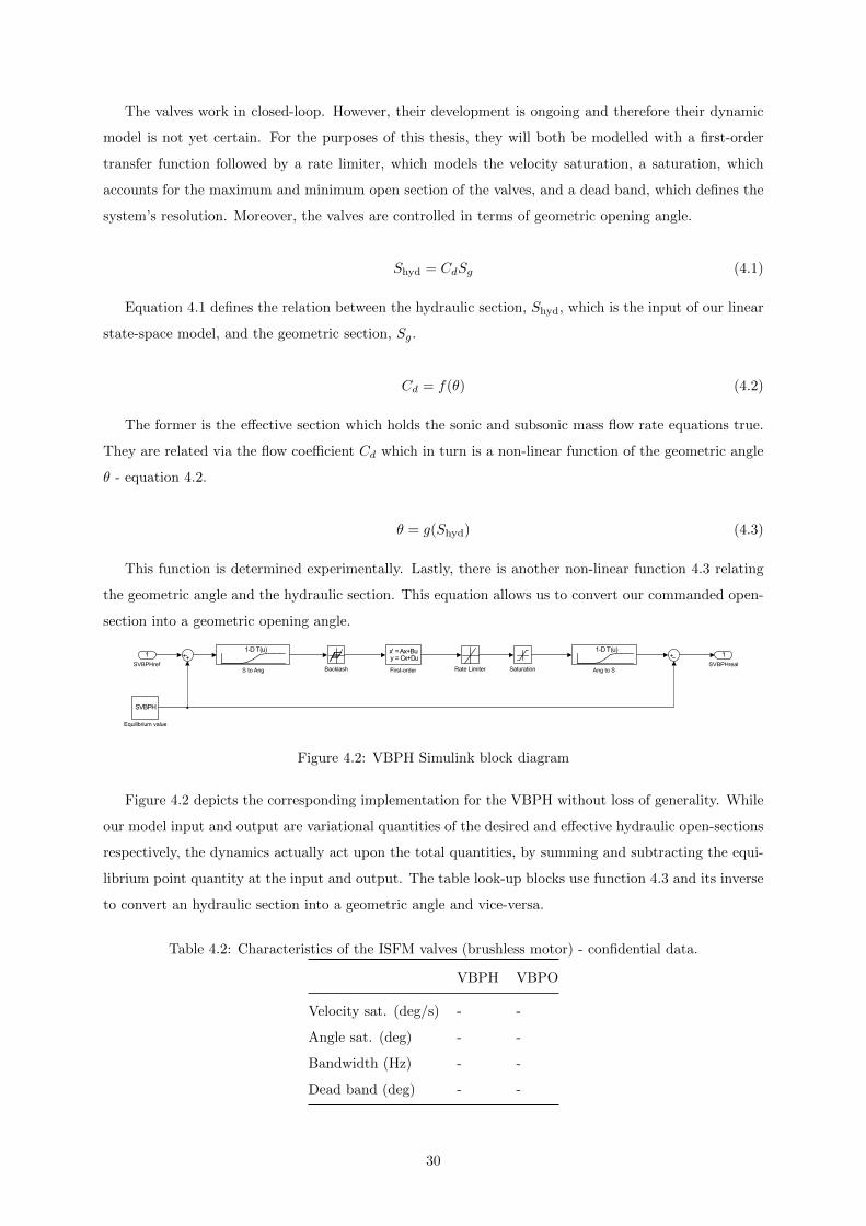
The valves work in closed-loop. However, their development is ongoing and therefore their dynamic

model is not yet certain. For the purposes of this thesis, they will both be modelled with a first-order

transfer function followed by a rate limiter, which models the velocity saturation, a saturation, which

accounts for the maximum and minimum open section of the valves, and a dead band, which defines the

system’s resolution. Moreover, the valves are controlled in terms of geometric opening angle.

Shyd = CdSg (4.1)

Equation 4.1 defines the relation between the hydraulic section, Shyd, which is the input of our linear

state-space model, and the geometric section, Sg.

Cd = f(θ) (4.2)

The former is the effective section which holds the sonic and subsonic mass flow rate equations true.

They are related via the flow coefficient Cd which in turn is a non-linear function of the geometric angle

θ - equation 4.2.

θ = g(Shyd) (4.3)

This function is determined experimentally. Lastly, there is another non-linear function 4.3 relating

the geometric angle and the hydraulic section. This equation allows us to convert our commanded open-

section into a geometric opening angle.

1

SVBPHreal

1

SVBPHref

1-D T(u)

S to Ang

1-D T(u)

Ang to SRate Limiter

SVBPH

Equilibrium value

x' = Ax+Bu y = Cx+Du

First-order SaturationBacklash

Figure 4.2: VBPH Simulink block diagram

Figure 4.2 depicts the corresponding implementation for the VBPH without loss of generality. While

our model input and output are variational quantities of the desired and effective hydraulic open-sections

respectively, the dynamics actually act upon the total quantities, by summing and subtracting the equi-

librium point quantity at the input and output. The table look-up blocks use function 4.3 and its inverse

to convert an hydraulic section into a geometric angle and vice-versa.

Table 4.2: Characteristics of the ISFM valves (brushless motor) - confidential data.

VBPH VBPO

Velocity sat. (deg/s) - -

Angle sat. (deg) - -

Bandwidth (Hz) - -

Dead band (deg) - -

30

4.4 VINCI Governing Equations Linearization

A priori, it is known that we will have a 2× 2 MIMO system, with the chamber pressure and mixture

ratio as controlled outputs and the two valves’ sections as controlled inputs. As noted in section 4.2 the

VINCI engine has an expander thermodynamic cycle and is therefore coupled, which not only increases

the difficulty but also allows us to tackle a more general problem.

One of the objectives of this thesis is to obtain an analytic linear model of the VINCI engine around

the nominal equilibrium point. Our approach thus consists of linearizing the governing equations for each

of the elements that compose the engine around a generic operating point - for instance the pump, the

turbine and the combustion chamber. Because we don’t have access to an explicit non-linear state-space

formulation, it is not possible to simply calculate the gradients at the equilibrium point. Nor is it possible,

for that matter, to perform a numerical linearization of the non-linear model in CARINS. Recoding the

model equations in another tool was also out of scope due to the complexity of the full model, namely of

the combustion phenomena.

Several sub-systems participate in the modelling of the engine. Among them turbines, pumps, liquid

cavities, ideal gas cavities, liquid orifices, ideal gas orifices, adiabatic pipes, a regenerative circuit and a

combustion chamber (approximately 60 elements). Their governing equations, along with the necessary

hypothesis, assumptions and nomenclature, are confidential and will therefore not be presented here. An

exception is made for the adiabatic pipes so as to illustrate the developed work (model extracted from

CNES internal documentation).

The ideal gas law is used instead of the real gas tables. Density is supposed constant in liquid state.

The assembly of the linearized equations in order to obtain a classical linear state-space formulation

is discussed in the next section.

Adiabatic Pipes

Pipes transport the state of the flow and calculate solely the mass-flow rate at the exit of a cavity or

a cavity-like element. This model stands both for liquid and gas flows. Here is a list of hypothesis that

were made:

1. The diameter of the pipe is significantly smaller than its length;

2. The pipe has a constant cross section;

3. The flow is incompressible, adiabatic and isothermal;

Under these assumptions, the non-linear model which describes this element in CARINS is given by

equations 4.4.

dmdt = S

L (pe − ps − kp+12ρeS2 )m2

Ts = Te

ρs = ρe

(4.4)

where

31

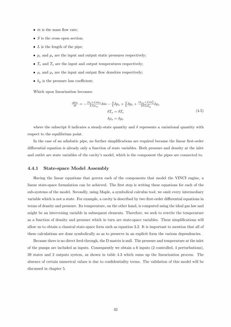
• m is the mass flow rate;

• S is the cross open section;

• L is the length of the pipe;

• pe and ps are the input and output static pressures respectively;

• Te and Ts are the input and output temperatures respectively;

• ρe and ρs are the input and output flow densities respectively;

• kp is the pressure loss coefficient;

Which upon linearization becomes:

dδmdt = − (kp+1)m0

LSρe0δm− S

Lδps + SLδpe +

(kp0+1)m20

2SLρ2e0δρe

δTs = δTe

δρs = δρe

(4.5)

where the subscript 0 indicates a steady-state quantity and δ represents a variational quantity with

respect to the equilibrium point.

In the case of an adiabatic pipe, no further simplifications are required because the linear first-order

differential equation is already only a function of state variables. Both pressure and density at the inlet

and outlet are state variables of the cavity’s model, which is the component the pipes are connected to.

4.4.1 State-space Model Assembly

Having the linear equations that govern each of the components that model the VINCI engine, a

linear state-space formulation can be achieved. The first step is writing these equations for each of the

sub-systems of the model. Secondly, using Maple, a symbolical calculus tool, we omit every intermediary

variable which is not a state. For example, a cavity is described by two first-order differential equations in

terms of density and pressure. Its temperature, on the other hand, is computed using the ideal gas law and

might be an intervening variable in subsequent elements. Therefore, we seek to rewrite the temperature

as a function of density and pressure which in turn are state-space variables. These simplifications will

allow us to obtain a classical state-space form such as equation 3.2. It is important to mention that all of

these calculations are done symbolically so as to preserve in an explicit form the various dependencies.

Because there is no direct feed-through, the D matrix is null. The pressure and temperature at the inlet

of the pumps are included as inputs. Consequently we obtain a 6 inputs (2 controlled, 4 perturbations),

39 states and 2 outputs system, as shown in table 4.3 which sums up the linearization process. The

absence of certain numerical values is due to confidentiality terms. The validation of this model will be

discussed in chapter 5.

32

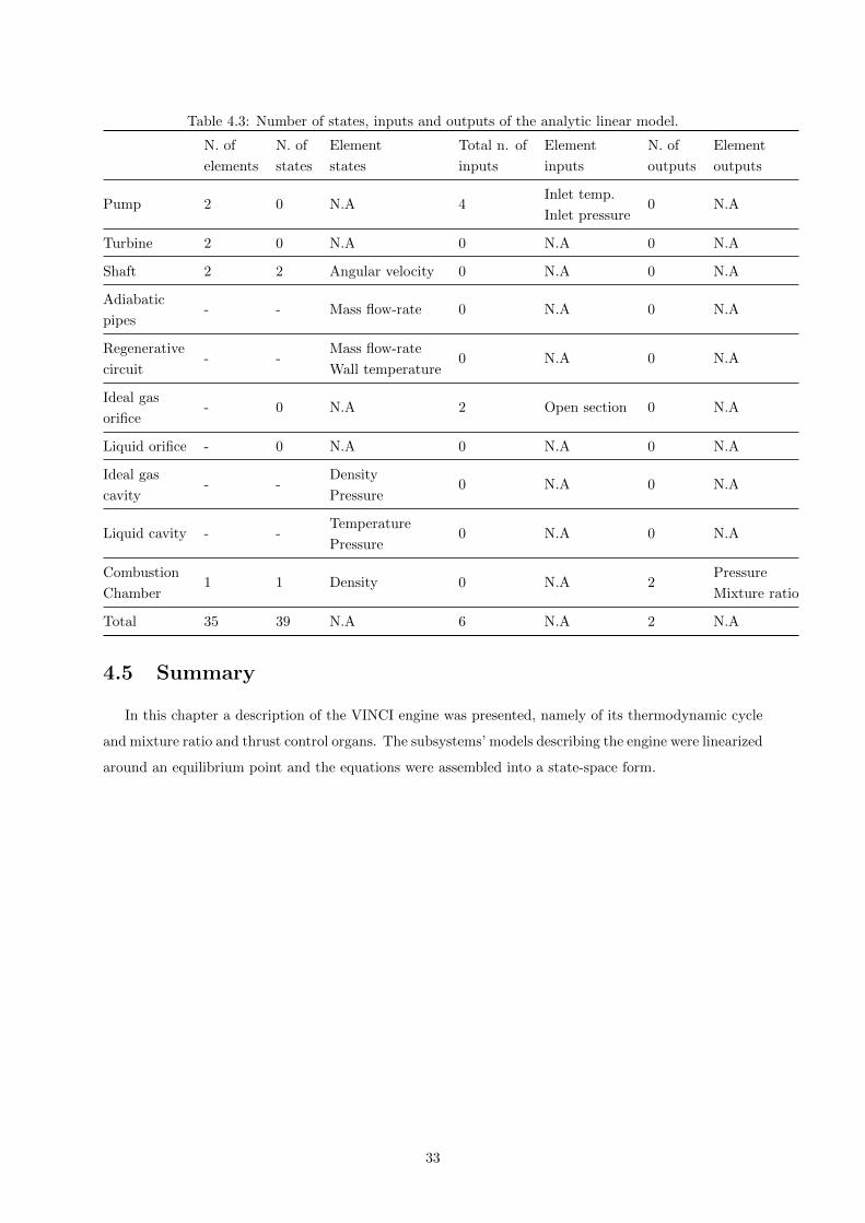
Table 4.3: Number of states, inputs and outputs of the analytic linear model.

N. of

elements

N. of

states

Element

states

Total n. of

inputs

Element

inputs

N. of

outputs

Element

outputs

Pump 2 0 N.A 4Inlet temp.

Inlet pressure0 N.A

Turbine 2 0 N.A 0 N.A 0 N.A

Shaft 2 2 Angular velocity 0 N.A 0 N.A

Adiabatic

pipes- - Mass flow-rate 0 N.A 0 N.A

Regenerative

circuit- -

Mass flow-rate

Wall temperature0 N.A 0 N.A

Ideal gas

orifice- 0 N.A 2 Open section 0 N.A

Liquid orifice - 0 N.A 0 N.A 0 N.A

Ideal gas

cavity- -

Density

Pressure0 N.A 0 N.A

Liquid cavity - -Temperature

Pressure0 N.A 0 N.A

Combustion

Chamber1 1 Density 0 N.A 2

Pressure

Mixture ratio

Total 35 39 N.A 6 N.A 2 N.A

4.5 Summary

In this chapter a description of the VINCI engine was presented, namely of its thermodynamic cycle

and mixture ratio and thrust control organs. The subsystems’ models describing the engine were linearized

around an equilibrium point and the equations were assembled into a state-space form.

33

34

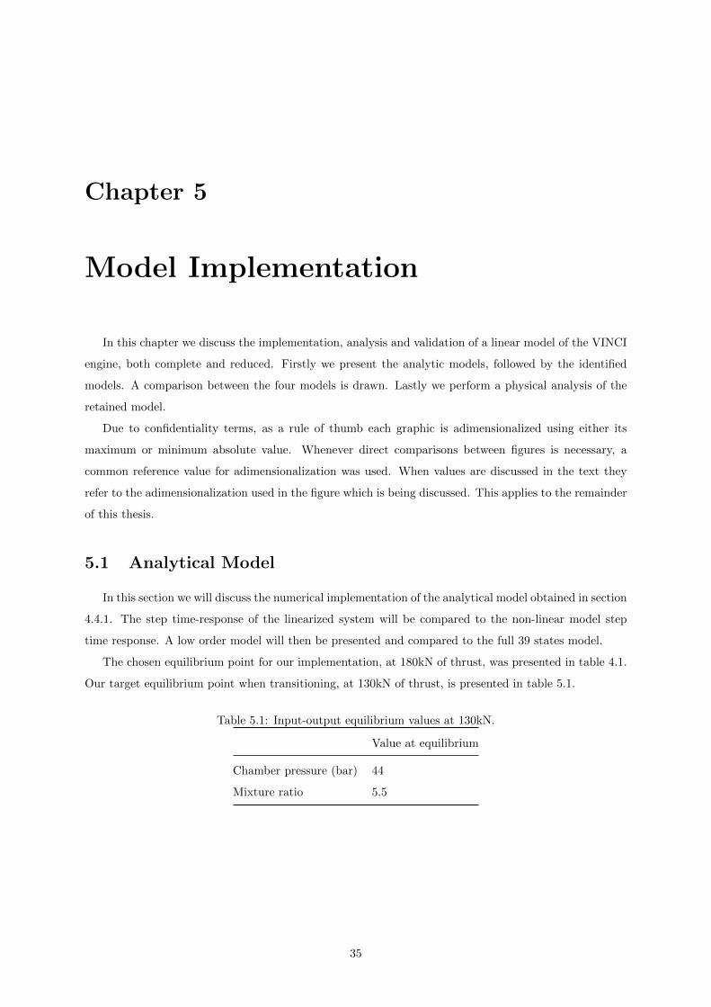
Chapter 5

Model Implementation

In this chapter we discuss the implementation, analysis and validation of a linear model of the VINCI

engine, both complete and reduced. Firstly we present the analytic models, followed by the identified

models. A comparison between the four models is drawn. Lastly we perform a physical analysis of the

retained model.

Due to confidentiality terms, as a rule of thumb each graphic is adimensionalized using either its

maximum or minimum absolute value. Whenever direct comparisons between figures is necessary, a

common reference value for adimensionalization was used. When values are discussed in the text they

refer to the adimensionalization used in the figure which is being discussed. This applies to the remainder

of this thesis.

5.1 Analytical Model

In this section we will discuss the numerical implementation of the analytical model obtained in section

4.4.1. The step time-response of the linearized system will be compared to the non-linear model step

time response. A low order model will then be presented and compared to the full 39 states model.

The chosen equilibrium point for our implementation, at 180kN of thrust, was presented in table 4.1.

Our target equilibrium point when transitioning, at 130kN of thrust, is presented in table 5.1.

Table 5.1: Input-output equilibrium values at 130kN.

Value at equilibrium

Chamber pressure (bar) 44

Mixture ratio 5.5

35

5.1.1 Complete Model

The numerical implementation of the full 39 states model was performed in MATLAB. Hereafter we

compare the time responses of the linear and non-linear systems, the quantities being variational with

respect to the 180kN regime.

The time-response to a VBPH section step in figure 5.1 presents a transient profile which fits that

of the non-linear model. However, both settling time and damping are inadequate. Moreover, the static

gain does not match our reference model.

Time0 0.1 0.2 0.3 0.4 0.5 0.6 0.7 0.8 0.9 1

Cha

mbe

r pr

essu

re

-1

-0.8

-0.6

-0.4

-0.2

0

Non-linear modelFull linear model

(a) Chamber pressure

Time0 0.1 0.2 0.3 0.4 0.5 0.6 0.7 0.8 0.9 1

Mix

ture

rat

io

-1

-0.8

-0.6

-0.4

-0.2

0

Non-linear modelFull linear model

(b) Mixture ratio

Figure 5.1: Linear and non-linear models time-response comparison to a VBPH section step of 20% ofthe nominal value at t = 0.

The time-response to a VBPO section step in figure 5.2, in agreement with what was seen for the

VBPH, has a transient response which generally fits that of the non-linear model. Both the chamber

pressure and the mixing ratio transfer functions present a static gain difference when compared to our

reference as well as a slight difference of response time. Moreover, the chamber pressure presents a

different damping than expected and an undesired non-minimum phase zero.

Time0.3 0.4 0.5 0.6 0.7 0.8 0.9 1

Cha

mbe

r pr

essu

re

-1

-0.8

-0.6

-0.4

-0.2

0 Non-linear modelFull linear model


Time0.3 0.4 0.5 0.6 0.7 0.8 0.9

Mix

ture

rat

io

-1

-0.8

-0.6

-0.4

-0.2

0Non-linear modelFull linear model

(b) Mixture ratio

Figure 5.2: Linear and non-linear models time-response comparison to a VBPO section step of 10% ofthe nominal value at t = 0.25.

36

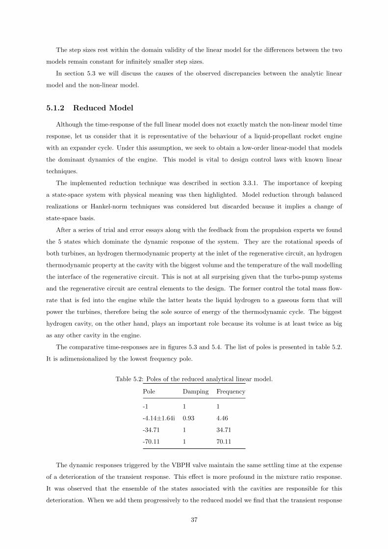
The step sizes rest within the domain validity of the linear model for the differences between the two

models remain constant for infinitely smaller step sizes.

In section 5.3 we will discuss the causes of the observed discrepancies between the analytic linear

model and the non-linear model.

5.1.2 Reduced Model

Although the time-response of the full linear model does not exactly match the non-linear model time

response, let us consider that it is representative of the behaviour of a liquid-propellant rocket engine

with an expander cycle. Under this assumption, we seek to obtain a low-order linear-model that models

the dominant dynamics of the engine. This model is vital to design control laws with known linear

techniques.

The implemented reduction technique was described in section 3.3.1. The importance of keeping

a state-space system with physical meaning was then highlighted. Model reduction through balanced

realizations or Hankel-norm techniques was considered but discarded because it implies a change of

state-space basis.

After a series of trial and error essays along with the feedback from the propulsion experts we found

the 5 states which dominate the dynamic response of the system. They are the rotational speeds of

both turbines, an hydrogen thermodynamic property at the inlet of the regenerative circuit, an hydrogen

thermodynamic property at the cavity with the biggest volume and the temperature of the wall modelling

the interface of the regenerative circuit. This is not at all surprising given that the turbo-pump systems

and the regenerative circuit are central elements to the design. The former control the total mass flow-

rate that is fed into the engine while the latter heats the liquid hydrogen to a gaseous form that will

power the turbines, therefore being the sole source of energy of the thermodynamic cycle. The biggest

hydrogen cavity, on the other hand, plays an important role because its volume is at least twice as big

as any other cavity in the engine.

The comparative time-responses are in figures 5.3 and 5.4. The list of poles is presented in table 5.2.

It is adimensionalized by the lowest frequency pole.

Table 5.2: Poles of the reduced analytical linear model.

Pole Damping Frequency

-1 1 1

-4.14±1.64i 0.93 4.46

-34.71 1 34.71

-70.11 1 70.11

The dynamic responses triggered by the VBPH valve maintain the same settling time at the expense

of a deterioration of the transient response. This effect is more profound in the mixture ratio response.

It was observed that the ensemble of the states associated with the cavities are responsible for this

deterioration. When we add them progressively to the reduced model we find that the transient response

37

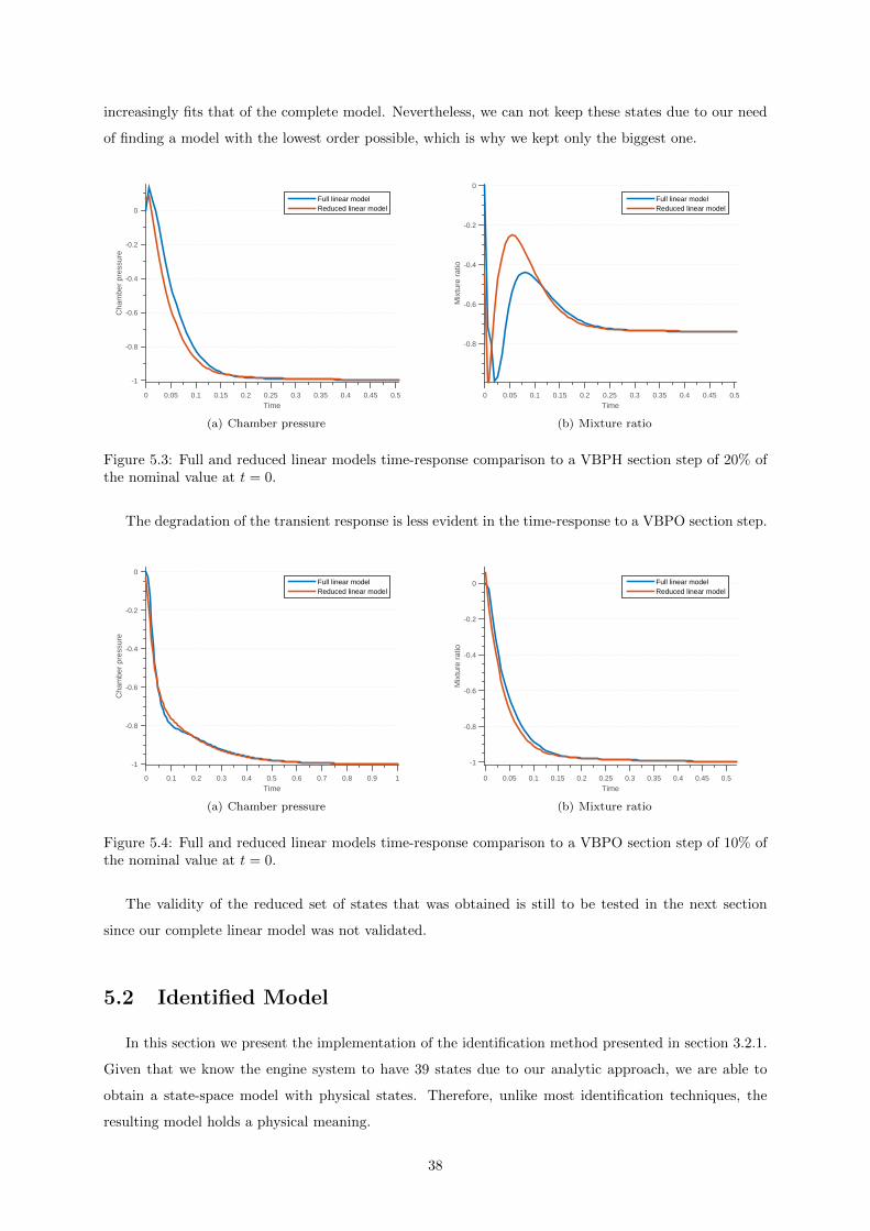
increasingly fits that of the complete model. Nevertheless, we can not keep these states due to our need

of finding a model with the lowest order possible, which is why we kept only the biggest one.

Time0 0.05 0.1 0.15 0.2 0.25 0.3 0.35 0.4 0.45 0.5

Cha

mbe

r pr

essu

re

-1

-0.8

-0.6

-0.4

-0.2

0

Full linear modelReduced linear model


Time0 0.05 0.1 0.15 0.2 0.25 0.3 0.35 0.4 0.45 0.5

Mix

ture

rat

io

-0.8

-0.6

-0.4

-0.2

0

Full linear modelReduced linear model

(b) Mixture ratio

Figure 5.3: Full and reduced linear models time-response comparison to a VBPH section step of 20% ofthe nominal value at t = 0.

The degradation of the transient response is less evident in the time-response to a VBPO section step.

Time0 0.1 0.2 0.3 0.4 0.5 0.6 0.7 0.8 0.9 1

Cha

mbe

r pr

essu

re

-1

-0.8

-0.6

-0.4

-0.2

0Full linear modelReduced linear model


Time0 0.05 0.1 0.15 0.2 0.25 0.3 0.35 0.4 0.45 0.5

Mix

ture

rat

io

-1

-0.8

-0.6

-0.4

-0.2

0 Full linear modelReduced linear model

(b) Mixture ratio

Figure 5.4: Full and reduced linear models time-response comparison to a VBPO section step of 10% ofthe nominal value at t = 0.

The validity of the reduced set of states that was obtained is still to be tested in the next section

since our complete linear model was not validated.

5.2 Identified Model

In this section we present the implementation of the identification method presented in section 3.2.1.

Given that we know the engine system to have 39 states due to our analytic approach, we are able to

obtain a state-space model with physical states. Therefore, unlike most identification techniques, the

resulting model holds a physical meaning.

38

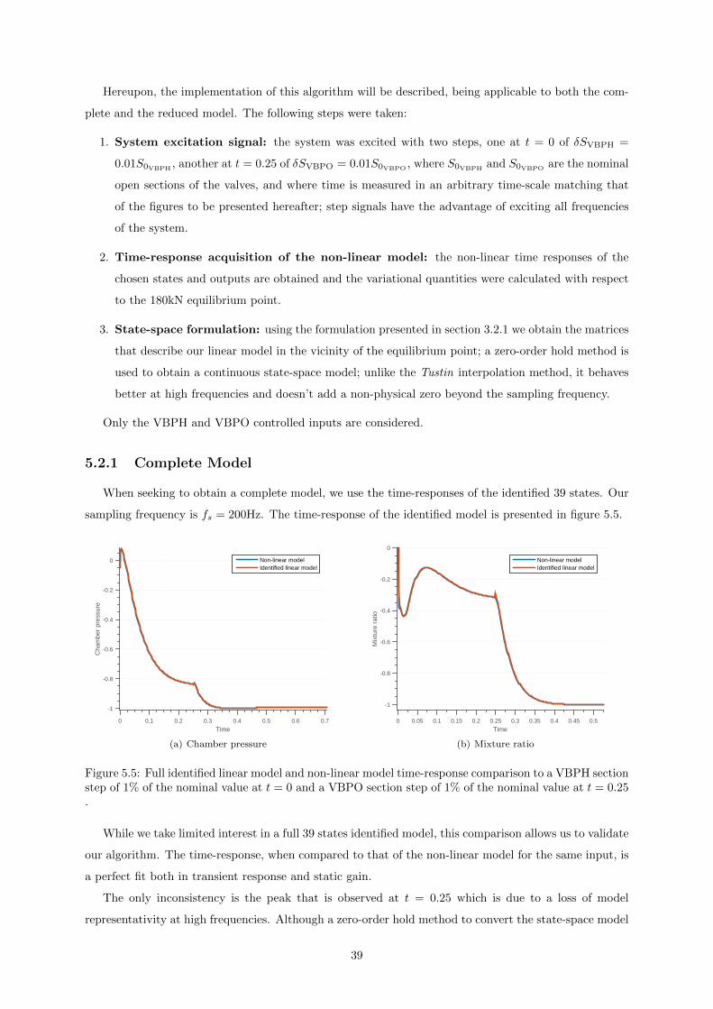
Hereupon, the implementation of this algorithm will be described, being applicable to both the com-

plete and the reduced model. The following steps were taken:

1. System excitation signal: the system was excited with two steps, one at t = 0 of δSVBPH =

0.01S0VBPH , another at t = 0.25 of δSVBPO = 0.01S0VBPO , where S0VBPH and S0VBPO are the nominal

open sections of the valves, and where time is measured in an arbitrary time-scale matching that

of the figures to be presented hereafter; step signals have the advantage of exciting all frequencies

of the system.

2. Time-response acquisition of the non-linear model: the non-linear time responses of the

chosen states and outputs are obtained and the variational quantities were calculated with respect

to the 180kN equilibrium point.

3. State-space formulation: using the formulation presented in section 3.2.1 we obtain the matrices

that describe our linear model in the vicinity of the equilibrium point; a zero-order hold method is

used to obtain a continuous state-space model; unlike the Tustin interpolation method, it behaves

better at high frequencies and doesn’t add a non-physical zero beyond the sampling frequency.

Only the VBPH and VBPO controlled inputs are considered.

5.2.1 Complete Model

When seeking to obtain a complete model, we use the time-responses of the identified 39 states. Our

sampling frequency is fs = 200Hz. The time-response of the identified model is presented in figure 5.5.

Time0 0.1 0.2 0.3 0.4 0.5 0.6 0.7

Cha

mbe

r pr

essu

re

-1

-0.8

-0.6

-0.4

-0.2

0 Non-linear modelIdentified linear model


Time0 0.05 0.1 0.15 0.2 0.25 0.3 0.35 0.4 0.45 0.5

Mix

ture

rat

io

-1

-0.8

-0.6

-0.4

-0.2

0

Non-linear modelIdentified linear model

(b) Mixture ratio

Figure 5.5: Full identified linear model and non-linear model time-response comparison to a VBPH sectionstep of 1% of the nominal value at t = 0 and a VBPO section step of 1% of the nominal value at t = 0.25.

While we take limited interest in a full 39 states identified model, this comparison allows us to validate

our algorithm. The time-response, when compared to that of the non-linear model for the same input, is

a perfect fit both in transient response and static gain.

The only inconsistency is the peak that is observed at t = 0.25 which is due to a loss of model

representativity at high frequencies. Although a zero-order hold method to convert the state-space model

39

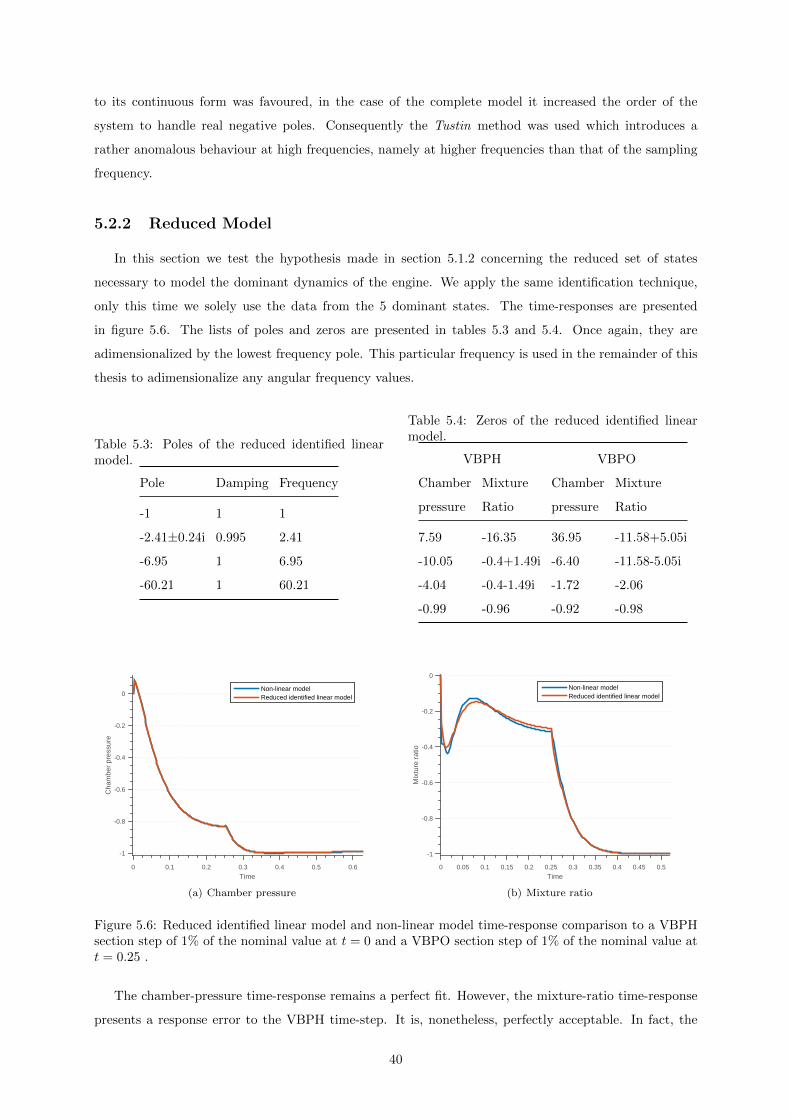
to its continuous form was favoured, in the case of the complete model it increased the order of the

system to handle real negative poles. Consequently the Tustin method was used which introduces a

rather anomalous behaviour at high frequencies, namely at higher frequencies than that of the sampling

frequency.

5.2.2 Reduced Model

In this section we test the hypothesis made in section 5.1.2 concerning the reduced set of states

necessary to model the dominant dynamics of the engine. We apply the same identification technique,

only this time we solely use the data from the 5 dominant states. The time-responses are presented

in figure 5.6. The lists of poles and zeros are presented in tables 5.3 and 5.4. Once again, they are

adimensionalized by the lowest frequency pole. This particular frequency is used in the remainder of this

thesis to adimensionalize any angular frequency values.

Table 5.3: Poles of the reduced identified linearmodel.


-1 1 1

-2.41±0.24i 0.995 2.41

-6.95 1 6.95

-60.21 1 60.21

Table 5.4: Zeros of the reduced identified linearmodel.

VBPH VBPO

Chamber

pressure

Mixture

Ratio

Chamber

pressure

Mixture

Ratio

7.59 -16.35 36.95 -11.58+5.05i

-10.05 -0.4+1.49i -6.40 -11.58-5.05i

-4.04 -0.4-1.49i -1.72 -2.06

-0.99 -0.96 -0.92 -0.98

Time0 0.1 0.2 0.3 0.4 0.5 0.6

Cha

mbe

r pr

essu

re

-1

-0.8

-0.6

-0.4

-0.2

0Non-linear modelReduced identified linear model


Time0 0.05 0.1 0.15 0.2 0.25 0.3 0.35 0.4 0.45 0.5

Mix

ture

rat

io

-1

-0.8

-0.6

-0.4

-0.2

0

Non-linear modelReduced identified linear model

(b) Mixture ratio

Figure 5.6: Reduced identified linear model and non-linear model time-response comparison to a VBPHsection step of 1% of the nominal value at t = 0 and a VBPO section step of 1% of the nominal value att = 0.25 .

The chamber-pressure time-response remains a perfect fit. However, the mixture-ratio time-response

presents a response error to the VBPH time-step. It is, nonetheless, perfectly acceptable. In fact, the

40

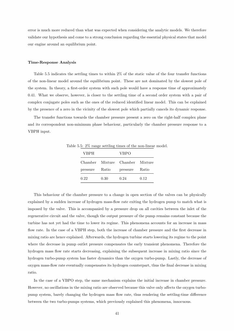
error is much more reduced than what was expected when considering the analytic models. We therefore

validate our hypothesis and come to a strong conclusion regarding the essential physical states that model

our engine around an equilibrium point.

Time-Response Analysis

Table 5.5 indicates the settling times to within 2% of the static value of the four transfer functions

of the non-linear model around the equilibrium point. These are not dominated by the slowest pole of

the system. In theory, a first-order system with such pole would have a response time of approximately

0.41. What we observe, however, is closer to the settling time of a second order system with a pair of

complex conjugate poles such as the ones of the reduced identified linear model. This can be explained

by the presence of a zero in the vicinity of the slowest pole which partially cancels its dynamic response.

The transfer functions towards the chamber pressure present a zero on the right-half complex plane

and its correspondent non-minimum phase behaviour, particularly the chamber pressure response to a

VBPH input.

Table 5.5: 2% range settling times of the non-linear model.

VBPH VBPO

Chamber

pressure

Mixture

Ratio

Chamber

pressure

Mixture

Ratio

0.22 0.30 0.24 0.12

This behaviour of the chamber pressure to a change in open section of the valves can be physically

explained by a sudden increase of hydrogen mass-flow rate exiting the hydrogen pump to match what is

imposed by the valve. This is accompanied by a pressure drop on all cavities between the inlet of the

regenerative circuit and the valve, though the output pressure of the pump remains constant because the

turbine has not yet had the time to lower its regime. This phenomena accounts for an increase in mass

flow rate. In the case of a VBPH step, both the increase of chamber pressure and the first decrease in

mixing ratio are hence explained. Afterwards, the hydrogen turbine starts lowering its regime to the point

where the decrease in pump outlet pressure compensates the early transient phenomena. Therefore the

hydrogen mass flow rate starts decreasing, explaining the subsequent increase in mixing ratio since the

hydrogen turbo-pump system has faster dynamics than the oxygen turbo-pump. Lastly, the decrease of

oxygen mass-flow rate eventually compensates its hydrogen counterpart, thus the final decrease in mixing

ratio.

In the case of a VBPO step, the same mechanism explains the initial increase in chamber pressure.

However, no oscillations in the mixing ratio are observed because this valve only affects the oxygen turbo-

pump system, barely changing the hydrogen mass flow rate, thus rendering the settling-time difference

between the two turbo-pumps systems, which previously explained this phenomena, innocuous.

41

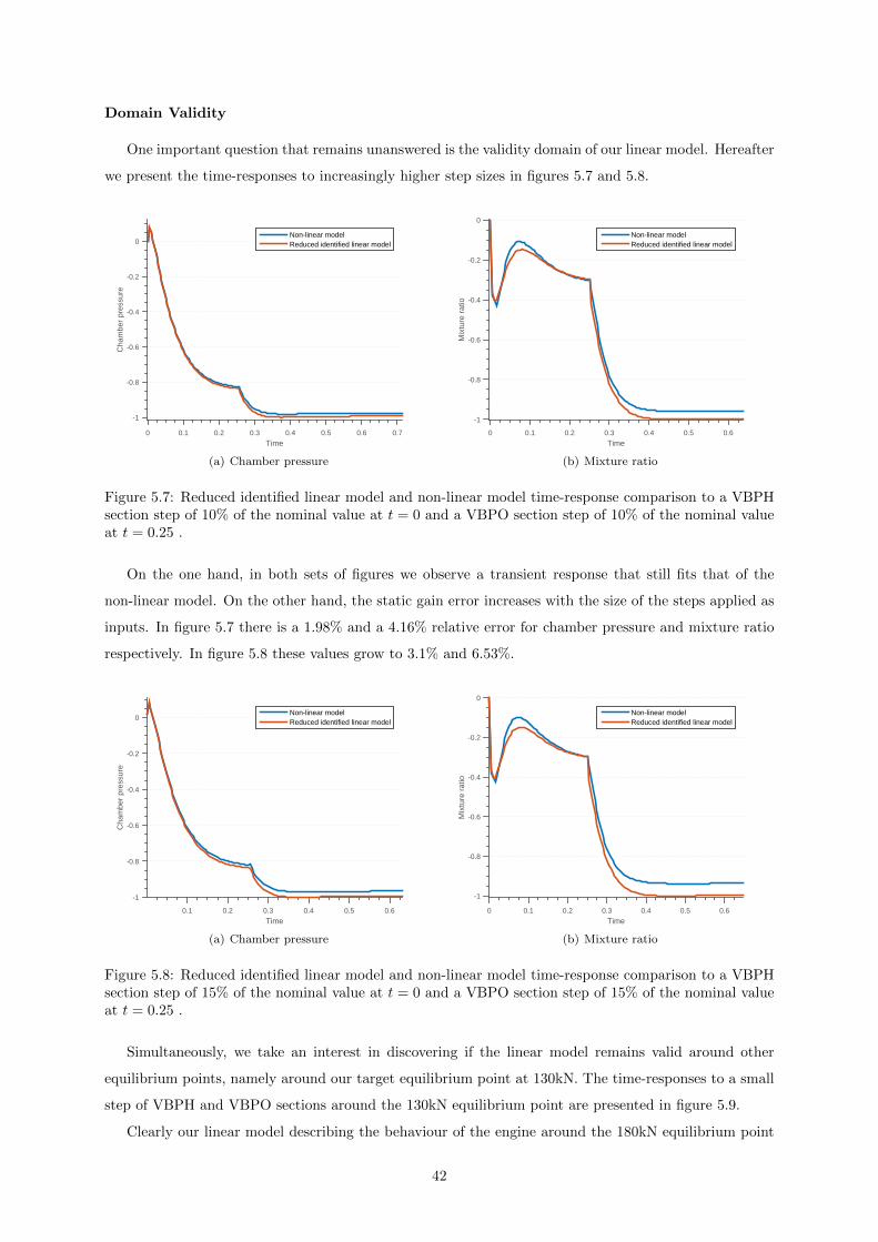
Domain Validity

One important question that remains unanswered is the validity domain of our linear model. Hereafter

we present the time-responses to increasingly higher step sizes in figures 5.7 and 5.8.

Time0 0.1 0.2 0.3 0.4 0.5 0.6 0.7

Cha

mbe

r pr

essu

re

-1

-0.8

-0.6

-0.4

-0.2



Time0 0.1 0.2 0.3 0.4 0.5 0.6

Mix

ture

rat

io

-1

-0.8

-0.6

-0.4

-0.2

0


(b) Mixture ratio

Figure 5.7: Reduced identified linear model and non-linear model time-response comparison to a VBPHsection step of 10% of the nominal value at t = 0 and a VBPO section step of 10% of the nominal valueat t = 0.25 .

On the one hand, in both sets of figures we observe a transient response that still fits that of the

non-linear model. On the other hand, the static gain error increases with the size of the steps applied as

inputs. In figure 5.7 there is a 1.98% and a 4.16% relative error for chamber pressure and mixture ratio

respectively. In figure 5.8 these values grow to 3.1% and 6.53%.

Time0.1 0.2 0.3 0.4 0.5 0.6

Cha

mbe

r pr

essu

re

-1

-0.8

-0.6

-0.4

-0.2



Time0 0.1 0.2 0.3 0.4 0.5 0.6

Mix

ture

rat

io

-1

-0.8

-0.6

-0.4

-0.2

0


(b) Mixture ratio

Figure 5.8: Reduced identified linear model and non-linear model time-response comparison to a VBPHsection step of 15% of the nominal value at t = 0 and a VBPO section step of 15% of the nominal valueat t = 0.25 .

Simultaneously, we take an interest in discovering if the linear model remains valid around other

equilibrium points, namely around our target equilibrium point at 130kN. The time-responses to a small

step of VBPH and VBPO sections around the 130kN equilibrium point are presented in figure 5.9.

Clearly our linear model describing the behaviour of the engine around the 180kN equilibrium point

42

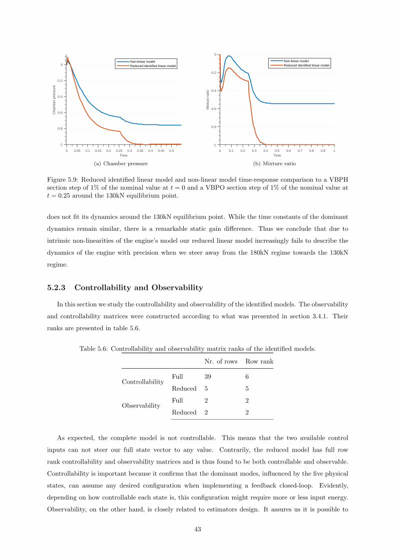
Time0 0.05 0.1 0.15 0.2 0.25 0.3 0.35 0.4 0.45 0.5

Cha

mbe

r pr

essu

re

-1

-0.8

-0.6

-0.4

-0.2



Time0 0.1 0.2 0.3 0.4 0.5 0.6 0.7 0.8 0.9 1

Mix

ture

rat

io

-1

-0.8

-0.6

-0.4

-0.2

0


(b) Mixture ratio

Figure 5.9: Reduced identified linear model and non-linear model time-response comparison to a VBPHsection step of 1% of the nominal value at t = 0 and a VBPO section step of 1% of the nominal value att = 0.25 around the 130kN equilibrium point.

does not fit its dynamics around the 130kN equilibrium point. While the time constants of the dominant

dynamics remain similar, there is a remarkable static gain difference. Thus we conclude that due to

intrinsic non-linearities of the engine’s model our reduced linear model increasingly fails to describe the

dynamics of the engine with precision when we steer away from the 180kN regime towards the 130kN

regime.

5.2.3 Controllability and Observability

In this section we study the controllability and observability of the identified models. The observability

and controllability matrices were constructed according to what was presented in section 3.4.1. Their

ranks are presented in table 5.6.

Table 5.6: Controllability and observability matrix ranks of the identified models.

Nr. of rows Row rank

ControllabilityFull 39 6

Reduced 5 5

ObservabilityFull 2 2

Reduced 2 2

As expected, the complete model is not controllable. This means that the two available control

inputs can not steer our full state vector to any value. Contrarily, the reduced model has full row

rank controllability and observability matrices and is thus found to be both controllable and observable.

Controllability is important because it confirms that the dominant modes, influenced by the five physical

states, can assume any desired configuration when implementing a feedback closed-loop. Evidently,

depending on how controllable each state is, this configuration might require more or less input energy.

Observability, on the other hand, is closely related to estimators design. It assures us it is possible to

43

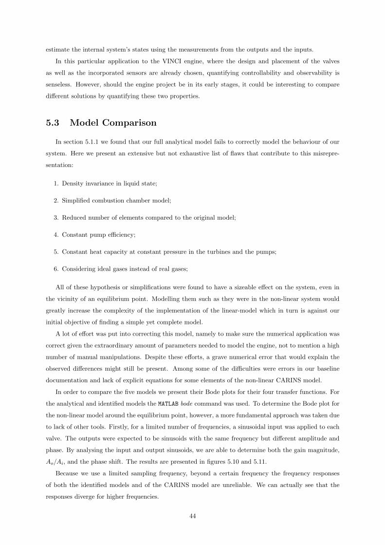
estimate the internal system’s states using the measurements from the outputs and the inputs.

In this particular application to the VINCI engine, where the design and placement of the valves

as well as the incorporated sensors are already chosen, quantifying controllability and observability is

senseless. However, should the engine project be in its early stages, it could be interesting to compare

different solutions by quantifying these two properties.

5.3 Model Comparison

In section 5.1.1 we found that our full analytical model fails to correctly model the behaviour of our

system. Here we present an extensive but not exhaustive list of flaws that contribute to this misrepre-

sentation:

1. Density invariance in liquid state;

2. Simplified combustion chamber model;

3. Reduced number of elements compared to the original model;

4. Constant pump efficiency;

5. Constant heat capacity at constant pressure in the turbines and the pumps;

6. Considering ideal gases instead of real gases;

All of these hypothesis or simplifications were found to have a sizeable effect on the system, even in

the vicinity of an equilibrium point. Modelling them such as they were in the non-linear system would

greatly increase the complexity of the implementation of the linear-model which in turn is against our

initial objective of finding a simple yet complete model.

A lot of effort was put into correcting this model, namely to make sure the numerical application was

correct given the extraordinary amount of parameters needed to model the engine, not to mention a high

number of manual manipulations. Despite these efforts, a grave numerical error that would explain the

observed differences might still be present. Among some of the difficulties were errors in our baseline

documentation and lack of explicit equations for some elements of the non-linear CARINS model.

In order to compare the five models we present their Bode plots for their four transfer functions. For

the analytical and identified models the MATLAB bode command was used. To determine the Bode plot for

the non-linear model around the equilibrium point, however, a more fundamental approach was taken due

to lack of other tools. Firstly, for a limited number of frequencies, a sinusoidal input was applied to each

valve. The outputs were expected to be sinusoids with the same frequency but different amplitude and

phase. By analysing the input and output sinusoids, we are able to determine both the gain magnitude,

Ao/Ai, and the phase shift. The results are presented in figures 5.10 and 5.11.

Because we use a limited sampling frequency, beyond a certain frequency the frequency responses

of both the identified models and of the CARINS model are unreliable. We can actually see that the

responses diverge for higher frequencies.

44

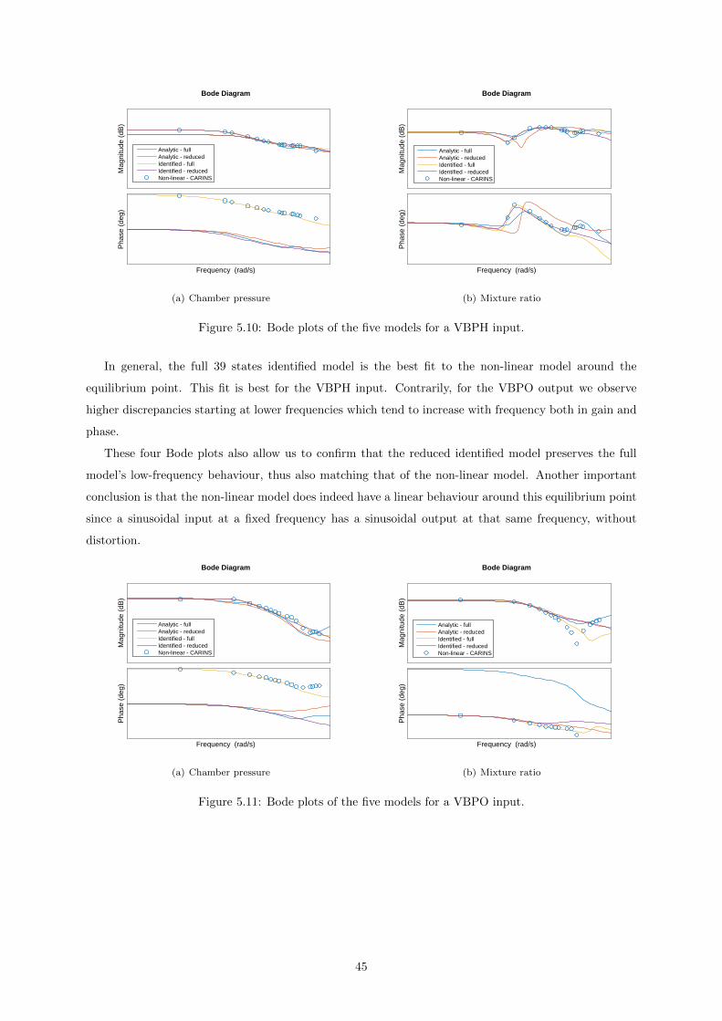
Mag

nitu

de (

dB)

Pha

se (

deg)

Analytic - fullAnalytic - reducedIdentified - fullIdentified - reducedNon-linear - CARINS

Bode Diagram

Frequency (rad/s)


Mag

nitu

de (

dB)

Pha

se (

deg)


Bode Diagram

Frequency (rad/s)

(b) Mixture ratio

Figure 5.10: Bode plots of the five models for a VBPH input.

In general, the full 39 states identified model is the best fit to the non-linear model around the

equilibrium point. This fit is best for the VBPH input. Contrarily, for the VBPO output we observe

higher discrepancies starting at lower frequencies which tend to increase with frequency both in gain and

phase.

These four Bode plots also allow us to confirm that the reduced identified model preserves the full

model’s low-frequency behaviour, thus also matching that of the non-linear model. Another important

conclusion is that the non-linear model does indeed have a linear behaviour around this equilibrium point

since a sinusoidal input at a fixed frequency has a sinusoidal output at that same frequency, without

distortion.

Mag

nitu

de (

dB)

Pha

se (

deg)


Bode Diagram

Frequency (rad/s)


Mag

nitu

de (

dB)

Pha

se (

deg)


Bode Diagram

Frequency (rad/s)

(b) Mixture ratio

Figure 5.11: Bode plots of the five models for a VBPO input.

45

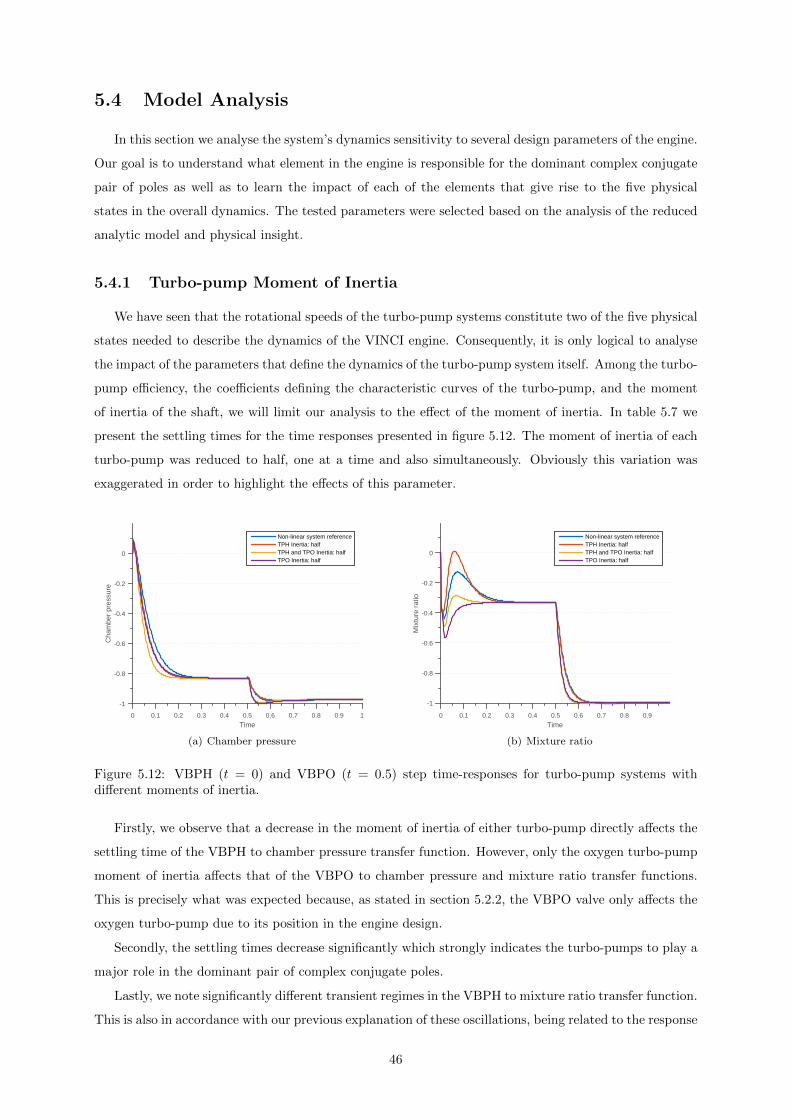
5.4 Model Analysis

In this section we analyse the system’s dynamics sensitivity to several design parameters of the engine.

Our goal is to understand what element in the engine is responsible for the dominant complex conjugate

pair of poles as well as to learn the impact of each of the elements that give rise to the five physical

states in the overall dynamics. The tested parameters were selected based on the analysis of the reduced

analytic model and physical insight.

5.4.1 Turbo-pump Moment of Inertia

We have seen that the rotational speeds of the turbo-pump systems constitute two of the five physical

states needed to describe the dynamics of the VINCI engine. Consequently, it is only logical to analyse

the impact of the parameters that define the dynamics of the turbo-pump system itself. Among the turbo-

pump efficiency, the coefficients defining the characteristic curves of the turbo-pump, and the moment

of inertia of the shaft, we will limit our analysis to the effect of the moment of inertia. In table 5.7 we

present the settling times for the time responses presented in figure 5.12. The moment of inertia of each

turbo-pump was reduced to half, one at a time and also simultaneously. Obviously this variation was

exaggerated in order to highlight the effects of this parameter.

Time0 0.1 0.2 0.3 0.4 0.5 0.6 0.7 0.8 0.9 1

Cha

mbe

r pr

essu

re

-1

-0.8

-0.6

-0.4

-0.2

0

Non-linear system referenceTPH Inertia: halfTPH and TPO Inertia: halfTPO Inertia: half


Time0 0.1 0.2 0.3 0.4 0.5 0.6 0.7 0.8 0.9

Mix

ture

rat

io

-1

-0.8

-0.6

-0.4

-0.2

0

Non-linear system referenceTPH Inertia: halfTPH and TPO Inertia: halfTPO Inertia: half

(b) Mixture ratio

Figure 5.12: VBPH (t = 0) and VBPO (t = 0.5) step time-responses for turbo-pump systems withdifferent moments of inertia.

Firstly, we observe that a decrease in the moment of inertia of either turbo-pump directly affects the

settling time of the VBPH to chamber pressure transfer function. However, only the oxygen turbo-pump

moment of inertia affects that of the VBPO to chamber pressure and mixture ratio transfer functions.

This is precisely what was expected because, as stated in section 5.2.2, the VBPO valve only affects the

oxygen turbo-pump due to its position in the engine design.

Secondly, the settling times decrease significantly which strongly indicates the turbo-pumps to play a

major role in the dominant pair of complex conjugate poles.

Lastly, we note significantly different transient regimes in the VBPH to mixture ratio transfer function.

This is also in accordance with our previous explanation of these oscillations, being related to the response

46

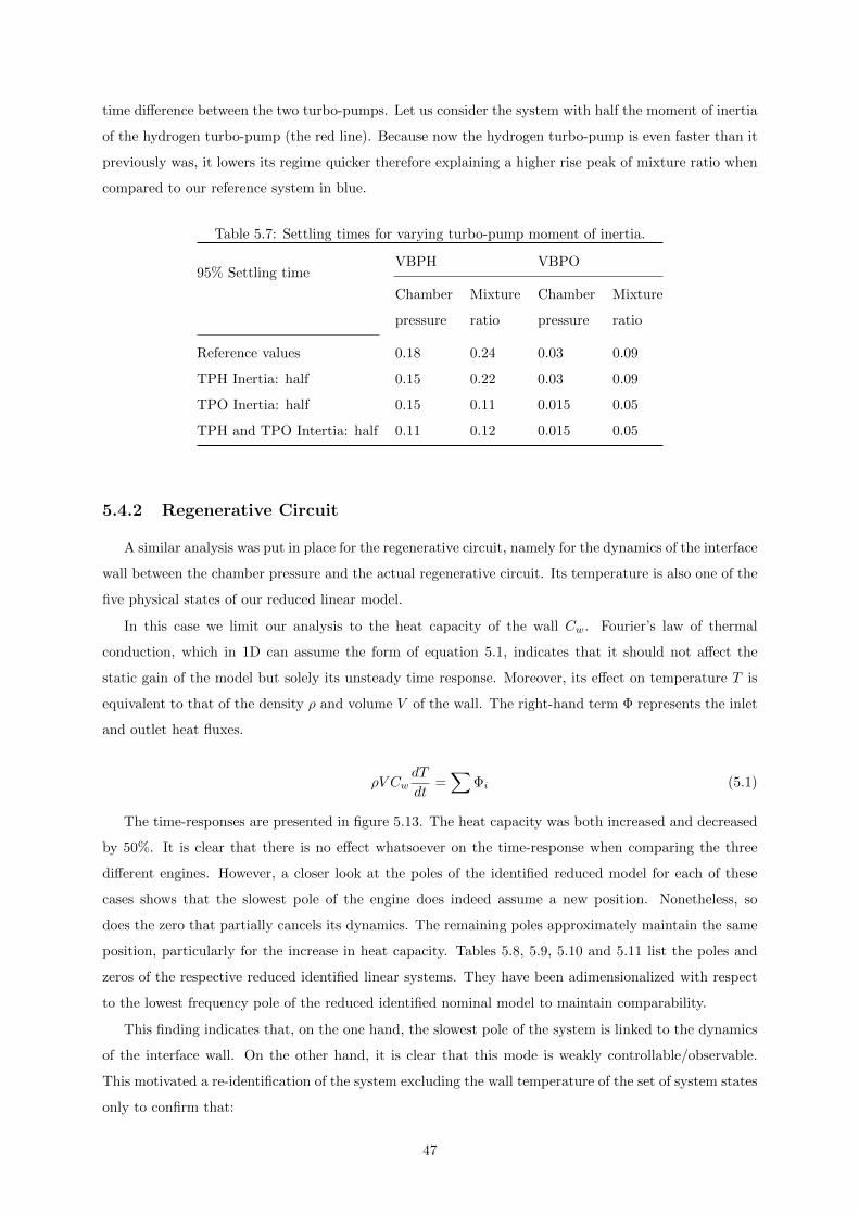
time difference between the two turbo-pumps. Let us consider the system with half the moment of inertia

of the hydrogen turbo-pump (the red line). Because now the hydrogen turbo-pump is even faster than it

previously was, it lowers its regime quicker therefore explaining a higher rise peak of mixture ratio when

compared to our reference system in blue.

Table 5.7: Settling times for varying turbo-pump moment of inertia.

95% Settling timeVBPH VBPO

Chamber

pressure

Mixture

ratio

Chamber

pressure

Mixture

ratio

Reference values 0.18 0.24 0.03 0.09

TPH Inertia: half 0.15 0.22 0.03 0.09

TPO Inertia: half 0.15 0.11 0.015 0.05

TPH and TPO Intertia: half 0.11 0.12 0.015 0.05

5.4.2 Regenerative Circuit

A similar analysis was put in place for the regenerative circuit, namely for the dynamics of the interface

wall between the chamber pressure and the actual regenerative circuit. Its temperature is also one of the

five physical states of our reduced linear model.

In this case we limit our analysis to the heat capacity of the wall Cw. Fourier’s law of thermal

conduction, which in 1D can assume the form of equation 5.1, indicates that it should not affect the

static gain of the model but solely its unsteady time response. Moreover, its effect on temperature T is

equivalent to that of the density ρ and volume V of the wall. The right-hand term Φ represents the inlet

and outlet heat fluxes.

ρV CwdT

dt=∑

Φi (5.1)

The time-responses are presented in figure 5.13. The heat capacity was both increased and decreased

by 50%. It is clear that there is no effect whatsoever on the time-response when comparing the three

different engines. However, a closer look at the poles of the identified reduced model for each of these

cases shows that the slowest pole of the engine does indeed assume a new position. Nonetheless, so

does the zero that partially cancels its dynamics. The remaining poles approximately maintain the same

position, particularly for the increase in heat capacity. Tables 5.8, 5.9, 5.10 and 5.11 list the poles and

zeros of the respective reduced identified linear systems. They have been adimensionalized with respect

to the lowest frequency pole of the reduced identified nominal model to maintain comparability.

This finding indicates that, on the one hand, the slowest pole of the system is linked to the dynamics

of the interface wall. On the other hand, it is clear that this mode is weakly controllable/observable.

This motivated a re-identification of the system excluding the wall temperature of the set of system states

only to confirm that:

47

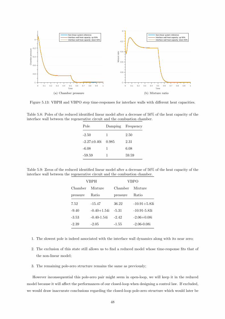
Time0 0.1 0.2 0.3 0.4 0.5 0.6 0.7 0.8 0.9 1

Cha

mbe

r pr

essu

re

-1

-0.8

-0.6

-0.4

-0.2

0

Non-linear system referenceInterface wall heat capacity: up 50%Interface wall heat capacity: down 50%


Time0 0.1 0.2 0.3 0.4 0.5 0.6 0.7 0.8 0.9 1

Mix

ture

rat

io

-1

-0.8

-0.6

-0.4

-0.2

0

Non-linear system referenceInterface wall heat capacity: up 50%Interface wall heat capacity: down 50%

(b) Mixture ratio

Figure 5.13: VBPH and VBPO step time-responses for interface walls with different heat capacities.

Table 5.8: Poles of the reduced identified linear model after a decrease of 50% of the heat capacity of theinterface wall between the regenerative circuit and the combustion chamber.


-2.50 1 2.50

-2.27±0.40i 0.985 2.31

-6.08 1 6.08

-59.59 1 59.59

Table 5.9: Zeros of the reduced identified linear model after a decrease of 50% of the heat capacity of theinterface wall between the regenerative circuit and the combustion chamber.

VBPH VBPO

Chamber

pressure

Mixture

Ratio

Chamber

pressure

Mixture

Ratio

7.52 -15.47 36.22 -10.91+5.83i

-9.40 -0.40+1.54i -5.31 -10.91-5.83i

-3.53 -0.40-1.54i -2.42 -2.06+0.08i

-2.39 -2.05 -1.55 -2.06-0.08i

1. The slowest pole is indeed associated with the interface wall dynamics along with its near zero;

2. The exclusion of this state still allows us to find a reduced model whose time-response fits that of

the non-linear model;

3. The remaining pole-zero structure remains the same as previously;

However inconsequential this pole-zero pair might seem in open-loop, we will keep it in the reduced

model because it will affect the performances of our closed-loop when designing a control law. If excluded,

we would draw inaccurate conclusions regarding the closed-loop pole-zero structure which would later be

48

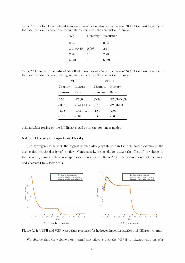
Table 5.10: Poles of the reduced identified linear model after an increase of 50% of the heat capacity ofthe interface wall between the regenerative circuit and the combustion chamber.


-0.64 1 0.64

-2.41±0.29i 0.993 2.41

-7.28 1 7.28

-60.21 1 60.21

Table 5.11: Zeros of the reduced identified linear model after an increase of 50% of the heat capacity ofthe interface wall between the regenerative circuit and the combustion chamber.

VBPH VBPO

Chamber

pressure

Mixture

Ratio

Chamber

pressure

Mixture

Ratio

7.50 -17.60 35.44 -12.03+5.33i

-10.30 -0.41+1.52i -6.73 -12.03-5.33i

-4.08 -0.41-1.52i -1.66 -2.06

-0.63 -0.63 -0.60 -0.63

evident when testing on the full linear model or on the non-linear model.

5.4.3 Hydrogen Injection Cavity

The hydrogen cavity with the biggest volume also plays its role in the dominant dynamics of the

engine through the density of the flow. Consequently, we sought to analyse the effect of its volume on

the overall dynamics. The time-responses are presented in figure 5.14. The volume was both increased

and decreased by a factor of 3.

Time0 0.1 0.2 0.3 0.4 0.5 0.6 0.7 0.8 0.9 1

Cha

mbe

r pr

essu

re

-1

-0.8

-0.6

-0.4

-0.2

0

Non-linear system referenceHydrogen injection cavity volume: x3Hydrogen injection cavity volume: /3


Time0 0.1 0.2 0.3 0.4 0.5 0.6 0.7 0.8 0.9 1

Mix

ture

rat

io

-1

-0.8

-0.6

-0.4

-0.2

0

Non-linear system referenceHydrogen injection cavity volume: x3Hydrogen injection cavity volume: /3

(b) Mixture ratio

Figure 5.14: VBPH and VBPO step time-responses for hydrogen injection cavities with different volumes.

We observe that the volume’s only significant effect is over the VBPH to mixture ratio transfer

49

function, namely its transient time-response. Let us consider the volume increase by a factor of 3 for

example (red line). This increase causes a delay of the hydrogen mass-flow rate arriving at the chamber

thus explaining a smaller rise peak of mixture ratio when compared to our reference model.

5.4.4 Mode Analysis Summary

The effects of the volume of the liquid cavity at the inlet of the regenerative circuit, whose thermo-

dynamic state is our fifth and last physical state, were not evaluated in the previous subsections. It was

observed, by re-identification with exclusion of this state, that it is associated with the fastest mode of

our reduced model and that its main effect on the time-response is an enhanced modelling of the non-

minimum phase behaviour of the chamber pressure. This is coherent with the explanation provided in

section 5.2.2 for this behaviour. Even though this mode is at a considerably higher frequency than the

dominant one, it was decided to preserve it in the reduced model. On the one hand because it improves,

even if only slightly, our model’s time response representativity and on the other hand because it does

not interfere with the controller design process.

The main conclusions of this section are the following:

1. The turbo-pump systems are associated with the dominant complex conjugate pair of poles;

2. The moment of inertia of the turbo-pumps significantly affects the settling-time of the four transfer

functions;

3. The temperature of the interface wall of the regenerative circuit is associated with the slowest

pole, yet it is weakly controllable/observable, and therefore has no significant effect over the time-

response;

4. The volume of the biggest cavity plays a major role in the transient time-response of the VBPH to

mixture ratio transfer function by lagging the time-response of the hydrogen mass flow rate arriving

at the inlet of the combustion chamber;

5.5 Summary

In this chapter we discussed the implementation of analytic and identified linear models of the VINCI

engine, both complete and reduced. A sufficient set of states to describe the dominant dynamics of

the engine was deduced. The reduced identified model, being the most adequate for control law design

purposes, was analysed. A comparison in the frequency domain between the four obtained models was

drawn only to confirm the validity of both the complete and the reduced identified linear models. Lastly a

sensitivity analysis was performed in order to understand the physics behind the unsteady time-response

of the engine.

50

Chapter 6

Control Specifications

In order to have a well-posed control problem we need to define the specifications to be met by our

control law. It is worth noting that since the engine is still in development, several numeric values are

unavailable. However, we have nonetheless, to the best of our ability, fixated conservative values to

those parameters. Because they are subjected to confidentiality, we will abstain from presenting them

in this chapter, and will therefore only list the type of specifications that were set. In chapters 7 and

8 adimensionalized values are presented when necessary to discuss control law implementation and the

results.

Hereafter we discuss parameter uncertainty, domain variation of the input perturbations, failure

events, mechanical/thermal limitations of the components, transient and steady-state time-response,

stability margins, discretization frequency and sensor’s characteristics.

6.1 Transient and Steady-State Time-Response

The transient and steady-state time-response of the closed loop system will have to respect criteria

of the following type:

1. Maximum overshoot of chamber pressure and mixture ratio;

2. Maximum 95% settling-time for step-like corrections of chamber pressure and mixture ratio;

3. Equilibrium point transition 95% settling time (180kN to 130kN);

4. Maximum perturbation rejection time;

5. Minimum required chamber pressure and mixture ratio precision;

The equilibrium point transition time is constrained by a maximum acceptable rate of chamber pres-

sure provided by the engine manufacturer. The required precision, on the other hand, concerns the

bounds around a desired reference value at which point we no longer require the system to seek to reduce

the error between the reference and the output. It allows us to limit the functioning of the actuators -

through a dead-zone for example - thus reducing the energy consumption. Both the settling-time and

51

the required precision address the needs of the PAM system such as they were presented to us at this

point of the development.

6.2 Stability margins

The minimum required modulus margin is 0.5, a typical value found in the literature, namely in

[21]. This will limit the maximum amplification of the reference value to the setpoint error to 2. In

other words, the H-infinity norm of the sensitivity function such as it is defined in section 3.5 can not

be higher than 2 - ||S||∞ < 2. We seek to respect this specification for all possible engine models within

the uncertainty set during the robustness analysis. Because this analysis does not take into account all

sources of uncertainty, it is important to guarantee a safety margin capable of accommodating possible

stability deteriorations due to discretization and non-linearities, among others.

6.3 Discretization Frequency

At this stage of the project the controller is set to work at a fairly high frequency, for which no

discretization effects are expected given the bandwidth of the system. However, since this value is yet to

be fixed, we will seek to determine the minimum frequency for which we do not need to take into account

the discretization effects.

6.4 Sensor’s Characteristics

The VINCI engine possesses several sensors, among which there are 8 of particular interest:

1. Chamber pressure;

2. Rotational speed of the hydrogen turbine;

3. Rotational speed of the oxygen turbine;

4. VBPH opening angle;

5. VBPO opening angle;

6. Oxygen pump outlet pressure;

7. Hydrogen pump outlet pressure;

8. Temperature of the regenerative circuit.

Notably, there is nor a direct measurement of the mixture ratio neither of the hydrogen and oxygen

mass flow rates. These sensors are available during ground tests but at this point there are no plans to

embed them in the launcher during flight. Therefore these quantities need to be estimated. Within the

scope of this thesis we will focus on the modelling of the chamber pressure sensor and will also attribute

equivalent characteristics to a pseudo mixture ratio sensor.

52

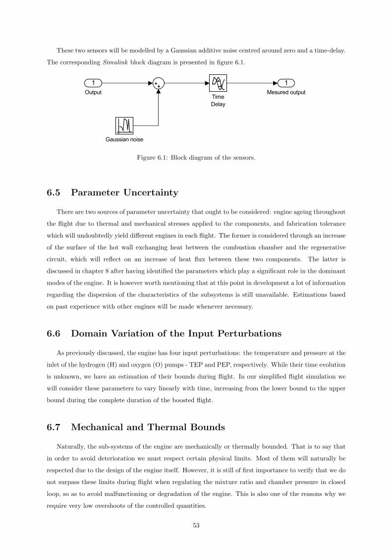
These two sensors will be modelled by a Gaussian additive noise centred around zero and a time-delay.

The corresponding Simulink block diagram is presented in figure 6.1.

1

Mesured output

1

Output

Gaussian noise

Time

Delay

Figure 6.1: Block diagram of the sensors.

6.5 Parameter Uncertainty

There are two sources of parameter uncertainty that ought to be considered: engine ageing throughout

the flight due to thermal and mechanical stresses applied to the components, and fabrication tolerance

which will undoubtedly yield different engines in each flight. The former is considered through an increase

of the surface of the hot wall exchanging heat between the combustion chamber and the regenerative

circuit, which will reflect on an increase of heat flux between these two components. The latter is

discussed in chapter 8 after having identified the parameters which play a significant role in the dominant

modes of the engine. It is however worth mentioning that at this point in development a lot of information

regarding the dispersion of the characteristics of the subsystems is still unavailable. Estimations based

on past experience with other engines will be made whenever necessary.

6.6 Domain Variation of the Input Perturbations

As previously discussed, the engine has four input perturbations: the temperature and pressure at the

inlet of the hydrogen (H) and oxygen (O) pumps - TEP and PEP, respectively. While their time evolution

is unknown, we have an estimation of their bounds during flight. In our simplified flight simulation we

will consider these parameters to vary linearly with time, increasing from the lower bound to the upper

bound during the complete duration of the boosted flight.

6.7 Mechanical and Thermal Bounds

Naturally, the sub-systems of the engine are mechanically or thermally bounded. That is to say that

in order to avoid deterioration we must respect certain physical limits. Most of them will naturally be

respected due to the design of the engine itself. However, it is still of first importance to verify that we do

not surpass these limits during flight when regulating the mixture ratio and chamber pressure in closed

loop, so as to avoid malfunctioning or degradation of the engine. This is also one of the reasons why we

require very low overshoots of the controlled quantities.

53

Hereafter we list the parameters for which there exists a lower and upper bounds to be respected:

1. Oxygen and hydrogen turbines rotational speeds;

2. Chamber pressure and mixture ratio;

3. Oxygen and hydrogen turbines inlet temperature;

4. Oxygen and hydrogen pumps outlet pressure;

Lastly, we present the list of parameters for which there is only an upper bound to be respected:

1. Oxygen and hydrogen turbines inlet pressure;

2. Oxygen turbine outlet pressure;

3. Turbo-pump torque;

4. Oxygen and hydrogen injectors inlet pressure and pressure drop;

5. Regenerative circuit inlet pressure;

6.8 Failure Events

In extraordinary situations, one might need to handle significant failure events. Hereafter the short

list that will be considered:

1. Increase in the pressure loss coefficient of the hydrogen injector;

2. Increase in the pressure loss coefficient of the oxygen injector;

3. Decrease in the efficiency of the oxygen pump;

4. Decrease in the efficiency of the oxygen turbine;

5. Decrease in the efficiency of the hydrogen pump;

6. Decrease in the efficiency of the hydrogen turbine;

There are no established specifications for the robustness of the control law regarding these failure

events. They will therefore not be taken into account when designing the control law but will rather be

simulated a posteriori and an upper or lower allowable bound will be determined for each case.

6.9 Summary

In this chapter the control problem was defined by listing the specifications to be met. The objectives

of the controller are thus defined.

54

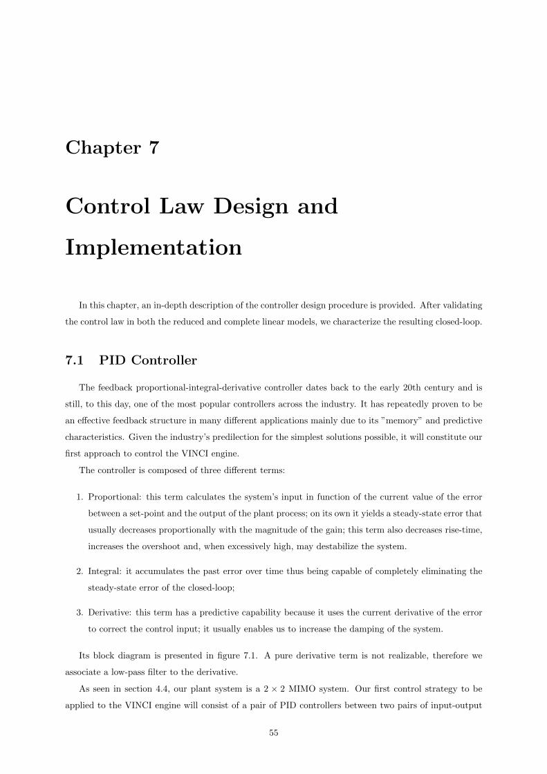
Chapter 7

Control Law Design and

Implementation

In this chapter, an in-depth description of the controller design procedure is provided. After validating

the control law in both the reduced and complete linear models, we characterize the resulting closed-loop.

7.1 PID Controller

The feedback proportional-integral-derivative controller dates back to the early 20th century and is

still, to this day, one of the most popular controllers across the industry. It has repeatedly proven to be

an effective feedback structure in many different applications mainly due to its ”memory” and predictive

characteristics. Given the industry’s predilection for the simplest solutions possible, it will constitute our

first approach to control the VINCI engine.

The controller is composed of three different terms:

1. Proportional: this term calculates the system’s input in function of the current value of the error

between a set-point and the output of the plant process; on its own it yields a steady-state error that

usually decreases proportionally with the magnitude of the gain; this term also decreases rise-time,

increases the overshoot and, when excessively high, may destabilize the system.

2. Integral: it accumulates the past error over time thus being capable of completely eliminating the

steady-state error of the closed-loop;

3. Derivative: this term has a predictive capability because it uses the current derivative of the error

to correct the control input; it usually enables us to increase the damping of the system.

Its block diagram is presented in figure 7.1. A pure derivative term is not realizable, therefore we

associate a low-pass filter to the derivative.

As seen in section 4.4, our plant system is a 2 × 2 MIMO system. Our first control strategy to be

applied to the VINCI engine will consist of a pair of PID controllers between two pairs of input-output

55

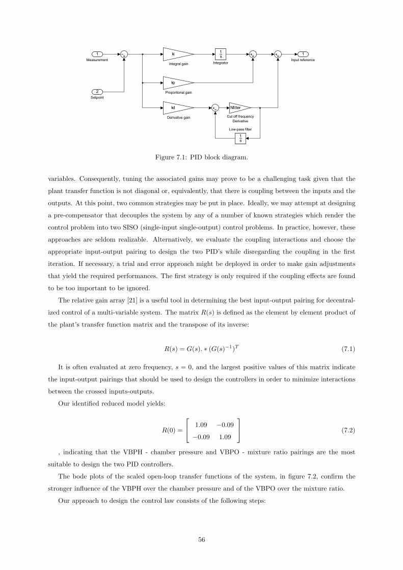
1

Input reference

1

Measurement

2

Setpoint

ki

Integral gain

1s

Integrator

kp

Proportional gain

kd

Derivative gain

Nfilter

Cut off frequency

Derivative

1s

Low-pass filter

Figure 7.1: PID block diagram.

variables. Consequently, tuning the associated gains may prove to be a challenging task given that the

plant transfer function is not diagonal or, equivalently, that there is coupling between the inputs and the

outputs. At this point, two common strategies may be put in place. Ideally, we may attempt at designing

a pre-compensator that decouples the system by any of a number of known strategies which render the

control problem into two SISO (single-input single-output) control problems. In practice, however, these

approaches are seldom realizable. Alternatively, we evaluate the coupling interactions and choose the

appropriate input-output pairing to design the two PID’s while disregarding the coupling in the first

iteration. If necessary, a trial and error approach might be deployed in order to make gain adjustments

that yield the required performances. The first strategy is only required if the coupling effects are found

to be too important to be ignored.

The relative gain array [21] is a useful tool in determining the best input-output pairing for decentral-

ized control of a multi-variable system. The matrix R(s) is defined as the element by element product of

the plant’s transfer function matrix and the transpose of its inverse:

R(s) = G(s). ∗ (G(s)−1)T (7.1)

It is often evaluated at zero frequency, s = 0, and the largest positive values of this matrix indicate

the input-output pairings that should be used to design the controllers in order to minimize interactions

between the crossed inputs-outputs.

Our identified reduced model yields:

R(0) =

1.09 −0.09

−0.09 1.09

(7.2)

, indicating that the VBPH - chamber pressure and VBPO - mixture ratio pairings are the most

suitable to design the two PID controllers.

The bode plots of the scaled open-loop transfer functions of the system, in figure 7.2, confirm the

stronger influence of the VBPH over the chamber pressure and of the VBPO over the mixture ratio.

Our approach to design the control law consists of the following steps:

56

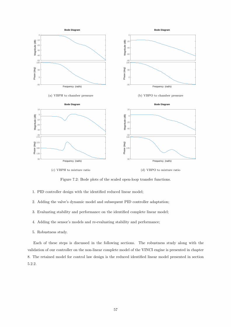
Mag

nitu

de (

dB)

-50

-40

-30

-20

-10

0P

hase

(de

g)

-90

0

90

180

Bode Diagram

Frequency (rad/s)

(a) VBPH to chamber pressure

Mag

nitu

de (

dB)

-80

-60

-40

-20

0

Pha

se (

deg)

-90

0

90

180

Bode Diagram

Frequency (rad/s)

(b) VBPO to chamber pressure

Mag

nitu

de (

dB)

-40

-30

-20

-10

0

10

Pha

se (

deg)

90

135

180

225

270

Bode Diagram

Frequency (rad/s)

(c) VBPH to mixture ratio

Mag

nitu

de (

dB)

-60

-40

-20

0

20

Pha

se (

deg)

90

135

180

Bode Diagram

Frequency (rad/s)

(d) VBPO to mixture ratio

Figure 7.2: Bode plots of the scaled open-loop transfer functions.

1. PID controller design with the identified reduced linear model;

2. Adding the valve’s dynamic model and subsequent PID controller adaptation;

3. Evaluating stability and performance on the identified complete linear model;

4. Adding the sensor’s models and re-evaluating stability and performance;

5. Robustness study.

Each of these steps is discussed in the following sections. The robustness study along with the

validation of our controller on the non-linear complete model of the VINCI engine is presented in chapter

8. The retained model for control law design is the reduced identified linear model presented in section

5.2.2.

57

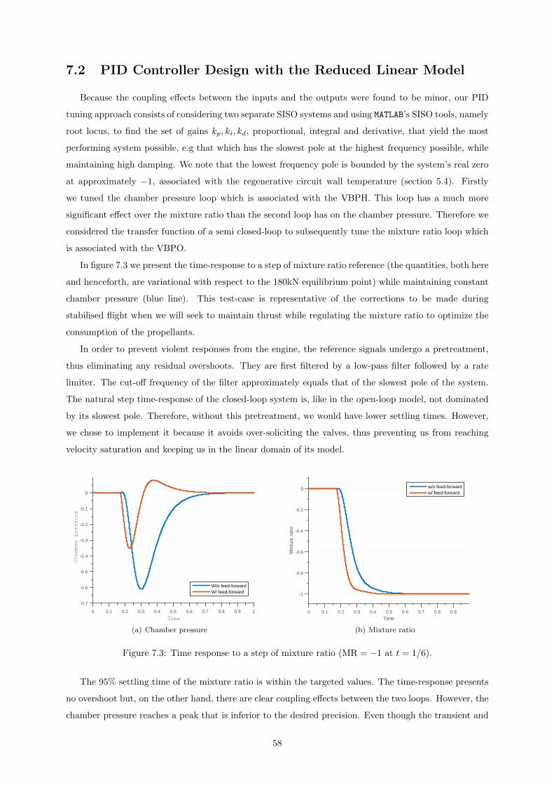
7.2 PID Controller Design with the Reduced Linear Model

Because the coupling effects between the inputs and the outputs were found to be minor, our PID

tuning approach consists of considering two separate SISO systems and using MATLAB’s SISO tools, namely

root locus, to find the set of gains kp, ki, kd, proportional, integral and derivative, that yield the most

performing system possible, e.g that which has the slowest pole at the highest frequency possible, while

maintaining high damping. We note that the lowest frequency pole is bounded by the system’s real zero

at approximately −1, associated with the regenerative circuit wall temperature (section 5.4). Firstly

we tuned the chamber pressure loop which is associated with the VBPH. This loop has a much more

significant effect over the mixture ratio than the second loop has on the chamber pressure. Therefore we

considered the transfer function of a semi closed-loop to subsequently tune the mixture ratio loop which

is associated with the VBPO.

In figure 7.3 we present the time-response to a step of mixture ratio reference (the quantities, both here

and henceforth, are variational with respect to the 180kN equilibrium point) while maintaining constant

chamber pressure (blue line). This test-case is representative of the corrections to be made during

stabilised flight when we will seek to maintain thrust while regulating the mixture ratio to optimize the

consumption of the propellants.

In order to prevent violent responses from the engine, the reference signals undergo a pretreatment,

thus eliminating any residual overshoots. They are first filtered by a low-pass filter followed by a rate

limiter. The cut-off frequency of the filter approximately equals that of the slowest pole of the system.

The natural step time-response of the closed-loop system is, like in the open-loop model, not dominated

by its slowest pole. Therefore, without this pretreatment, we would have lower settling times. However,

we chose to implement it because it avoids over-soliciting the valves, thus preventing us from reaching

velocity saturation and keeping us in the linear domain of its model.

Time

0 0.1 0.2 0.3 0.4 0.5 0.6 0.7 0.8 0.9 1

Chamber pressure

-0.7

-0.6

-0.5

-0.4

-0.3

-0.2

-0.1

0

W/o feed-forwardW/ feed-forward


Time0 0.1 0.2 0.3 0.4 0.5 0.6 0.7 0.8 0.9

Mix

ture

rat

io

-1

-0.8

-0.6

-0.4

-0.2

0 w/o feed-forwardw/ feed-forward

(b) Mixture ratio

Figure 7.3: Time response to a step of mixture ratio (MR = −1 at t = 1/6).

The 95% settling time of the mixture ratio is within the targeted values. The time-response presents

no overshoot but, on the other hand, there are clear coupling effects between the two loops. However, the

chamber pressure reaches a peak that is inferior to the desired precision. Even though the transient and

58

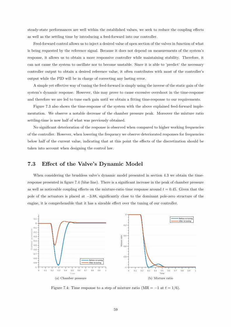
steady-state performances are well within the established values, we seek to reduce the coupling effects

as well as the settling time by introducing a feed-forward into our controller.

Feed-forward control allows us to inject a desired value of open section of the valves in function of what

is being requested by the reference signal. Because it does not depend on measurements of the system’s

response, it allows us to obtain a more responsive controller while maintaining stability. Therefore, it

can not cause the system to oscillate nor to become unstable. Since it is able to ’predict’ the necessary

controller output to obtain a desired reference value, it often contributes with most of the controller’s

output while the PID will be in charge of correcting any lasting error.

A simple yet effective way of tuning the feed-forward is simply using the inverse of the static gain of the

system’s dynamic response. However, this may prove to cause excessive overshoot in the time-response

and therefore we are led to tune each gain until we obtain a fitting time-response to our requirements.

Figure 7.3 also shows the time-response of the system with the above explained feed-forward imple-

mentation. We observe a notable decrease of the chamber pressure peak. Moreover the mixture ratio

settling-time is now half of what was previously obtained.

No significant deterioration of the response is observed when compared to higher working frequencies

of the controller. However, when lowering the frequency we observe deteriorated responses for frequencies

below half of the current value, indicating that at this point the effects of the discretization should be

taken into account when designing the control law.

7.3 Effect of the Valve’s Dynamic Model

When considering the brushless valve’s dynamic model presented in section 4.3 we obtain the time-

response presented in figure 7.4 (blue line). There is a significant increase in the peak of chamber pressure

as well as noticeable coupling effects on the mixture-ratio time response around t = 0.45. Given that the

pole of the actuators is placed at −3.88, significantly close to the dominant pole-zero structure of the

engine, it is comprehensible that it has a sizeable effect over the tuning of our controller.

Time

0 0.1 0.2 0.3 0.4 0.5 0.6 0.7 0.8 0.9 1

Chamber pressure

-1

-0.9

-0.8

-0.7

-0.6

-0.5

-0.4

-0.3

-0.2

-0.1

0

0.1

Before re-tuningAfter re-tuning


Time0 0.1 0.2 0.3 0.4 0.5 0.6 0.7 0.8 0.9 1

Mix

ture

rat

io

-1

-0.8

-0.6

-0.4

-0.2

0

Before re-tuningAfter re-tuning

(b) Mixture ratio

Figure 7.4: Time response to a step of mixture ratio (MR = −1 at t = 1/6).

59

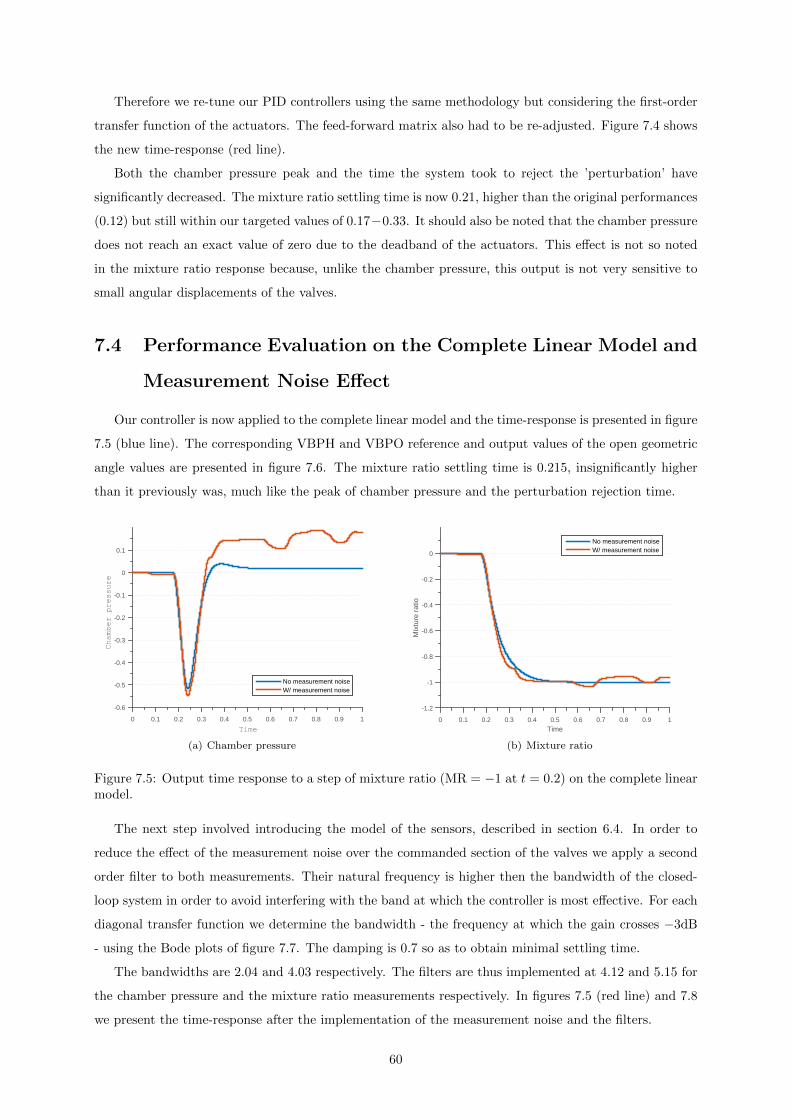
Therefore we re-tune our PID controllers using the same methodology but considering the first-order

transfer function of the actuators. The feed-forward matrix also had to be re-adjusted. Figure 7.4 shows

the new time-response (red line).

Both the chamber pressure peak and the time the system took to reject the ’perturbation’ have

significantly decreased. The mixture ratio settling time is now 0.21, higher than the original performances

(0.12) but still within our targeted values of 0.17−0.33. It should also be noted that the chamber pressure

does not reach an exact value of zero due to the deadband of the actuators. This effect is not so noted

in the mixture ratio response because, unlike the chamber pressure, this output is not very sensitive to

small angular displacements of the valves.

7.4 Performance Evaluation on the Complete Linear Model and

Measurement Noise Effect

Our controller is now applied to the complete linear model and the time-response is presented in figure

7.5 (blue line). The corresponding VBPH and VBPO reference and output values of the open geometric

angle values are presented in figure 7.6. The mixture ratio settling time is 0.215, insignificantly higher

than it previously was, much like the peak of chamber pressure and the perturbation rejection time.

Time

0 0.1 0.2 0.3 0.4 0.5 0.6 0.7 0.8 0.9 1

Chamber pressure

-0.6

-0.5

-0.4

-0.3

-0.2

-0.1

0

0.1

No measurement noiseW/ measurement noise


Time0 0.1 0.2 0.3 0.4 0.5 0.6 0.7 0.8 0.9 1

Mix

ture

rat

io

-1.2

-1

-0.8

-0.6

-0.4

-0.2

0

No measurement noiseW/ measurement noise

(b) Mixture ratio

Figure 7.5: Output time response to a step of mixture ratio (MR = −1 at t = 0.2) on the complete linearmodel.

The next step involved introducing the model of the sensors, described in section 6.4. In order to

reduce the effect of the measurement noise over the commanded section of the valves we apply a second

order filter to both measurements. Their natural frequency is higher then the bandwidth of the closed-

loop system in order to avoid interfering with the band at which the controller is most effective. For each

diagonal transfer function we determine the bandwidth - the frequency at which the gain crosses −3dB

- using the Bode plots of figure 7.7. The damping is 0.7 so as to obtain minimal settling time.

The bandwidths are 2.04 and 4.03 respectively. The filters are thus implemented at 4.12 and 5.15 for

the chamber pressure and the mixture ratio measurements respectively. In figures 7.5 (red line) and 7.8

we present the time-response after the implementation of the measurement noise and the filters.

60

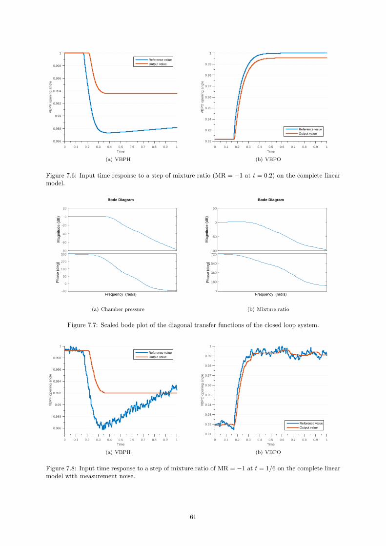
Time0 0.1 0.2 0.3 0.4 0.5 0.6 0.7 0.8 0.9 1

VB

PH

ope

ning

ang

le

0.986

0.988

0.99

0.992

0.994

0.996

0.998

1

Reference valueOutput value

(a) VBPH

Time0 0.1 0.2 0.3 0.4 0.5 0.6 0.7 0.8 0.9 1

VB

PO

ope

ning

ang

le

0.92

0.93

0.94

0.95

0.96

0.97

0.98

0.99

1


(b) VBPO

Figure 7.6: Input time response to a step of mixture ratio (MR = −1 at t = 0.2) on the complete linearmodel.

Mag

nitu

de (

dB)

-80

-60

-40

-20

0

20

Pha

se (

deg)

-90

0

90

180

270

360

Bode Diagram

Frequency (rad/s)


Mag

nitu

de (

dB)

-100

-50

0

50P

hase

(de

g)

0

180

360

540

720

Bode Diagram

Frequency (rad/s)

(b) Mixture ratio

Figure 7.7: Scaled bode plot of the diagonal transfer functions of the closed loop system.

Time0 0.1 0.2 0.3 0.4 0.5 0.6 0.7 0.8 0.9 1

VB

PH

ope

ning

ang

le

0.986

0.988

0.99

0.992

0.994

0.996

0.998

1


(a) VBPH

Time0 0.1 0.2 0.3 0.4 0.5 0.6 0.7 0.8 0.9 1

VB

PO

ope

ning

ang

le

0.91

0.92

0.93

0.94

0.95

0.96

0.97

0.98

0.99

1


(b) VBPO

Figure 7.8: Input time response to a step of mixture ratio of MR = −1 at t = 1/6 on the complete linearmodel with measurement noise.

61

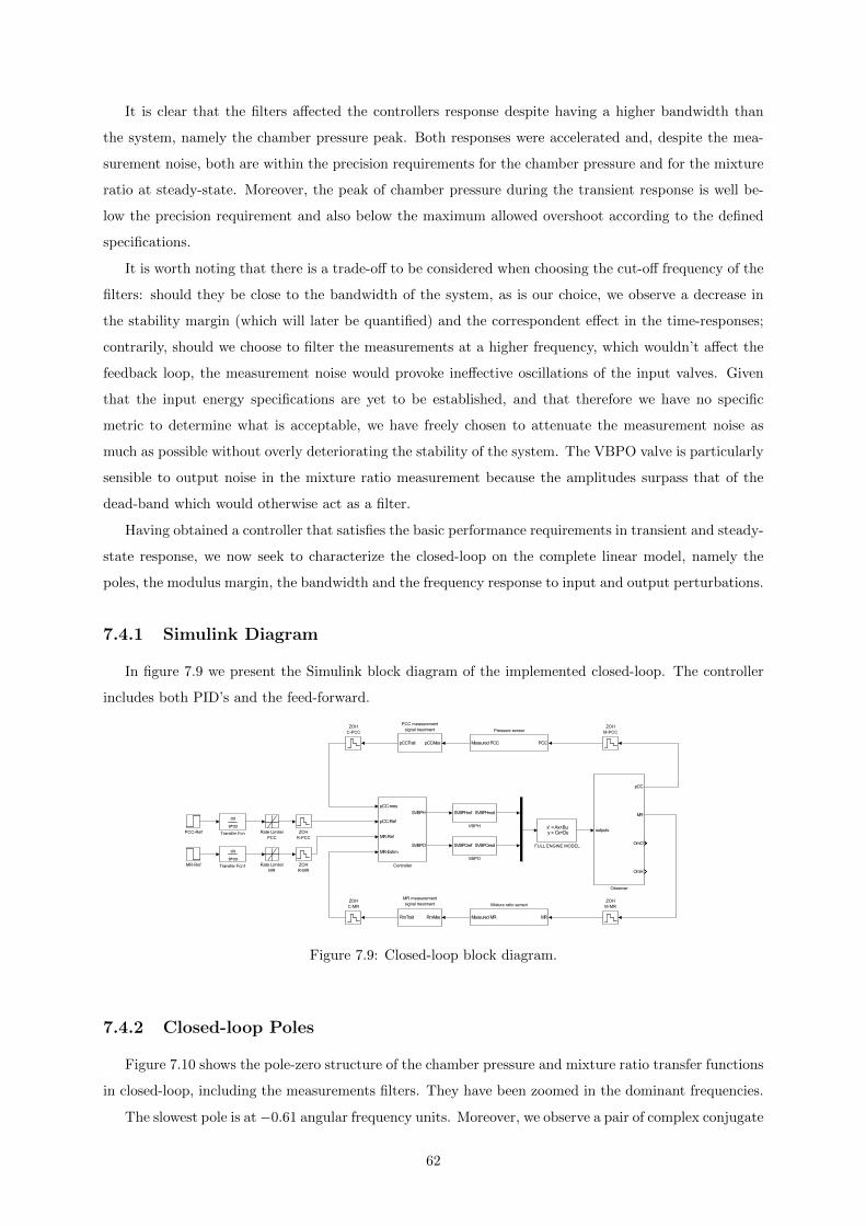
It is clear that the filters affected the controllers response despite having a higher bandwidth than

the system, namely the chamber pressure peak. Both responses were accelerated and, despite the mea-

surement noise, both are within the precision requirements for the chamber pressure and for the mixture

ratio at steady-state. Moreover, the peak of chamber pressure during the transient response is well be-

low the precision requirement and also below the maximum allowed overshoot according to the defined

specifications.

It is worth noting that there is a trade-off to be considered when choosing the cut-off frequency of the

filters: should they be close to the bandwidth of the system, as is our choice, we observe a decrease in

the stability margin (which will later be quantified) and the correspondent effect in the time-responses;

contrarily, should we choose to filter the measurements at a higher frequency, which wouldn’t affect the

feedback loop, the measurement noise would provoke ineffective oscillations of the input valves. Given

that the input energy specifications are yet to be established, and that therefore we have no specific

metric to determine what is acceptable, we have freely chosen to attenuate the measurement noise as

much as possible without overly deteriorating the stability of the system. The VBPO valve is particularly

sensible to output noise in the mixture ratio measurement because the amplitudes surpass that of the

dead-band which would otherwise act as a filter.

Having obtained a controller that satisfies the basic performance requirements in transient and steady-

state response, we now seek to characterize the closed-loop on the complete linear model, namely the

poles, the modulus margin, the bandwidth and the frequency response to input and output perturbations.

7.4.1 Simulink Diagram

In figure 7.9 we present the Simulink block diagram of the implemented closed-loop. The controller

includes both PID’s and the feed-forward.

x' = Ax+Bu y = Cx+Du

FULL ENGINE MODEL

SVBPHref SVBPHreal

VBPH

SVBPOref SVBPOreal

VBPO

PCC-Ref

MR-Ref

pCC-mes

pCC-Ref

MR-Ref

MR-Estim

SVBPH

SVBPO

Controller

outputs

pCC

MR

OmO

OmH

Observer

pCCMespCCTrait

PCC measurement

signal treatment

PCCMeasured PCC

Pressure sensor

RmMesRmTrait

MR measurement

signal treatment

MRMeasured MR

Mixture ratio sensor

Rate Limiter

PCC

Rate Limiter

MR

co

s+co

Transfer Fcn

co

s+co

Transfer Fcn1 ZOH

R-MR

ZOH

R-PCC

ZOH

C-PCC

ZOH

C-MR

ZOH

M-PCC

ZOH

M-MR

Figure 7.9: Closed-loop block diagram.

7.4.2 Closed-loop Poles

Figure 7.10 shows the pole-zero structure of the chamber pressure and mixture ratio transfer functions

in closed-loop, including the measurements filters. They have been zoomed in the dominant frequencies.

The slowest pole is at−0.61 angular frequency units. Moreover, we observe a pair of complex conjugate

62

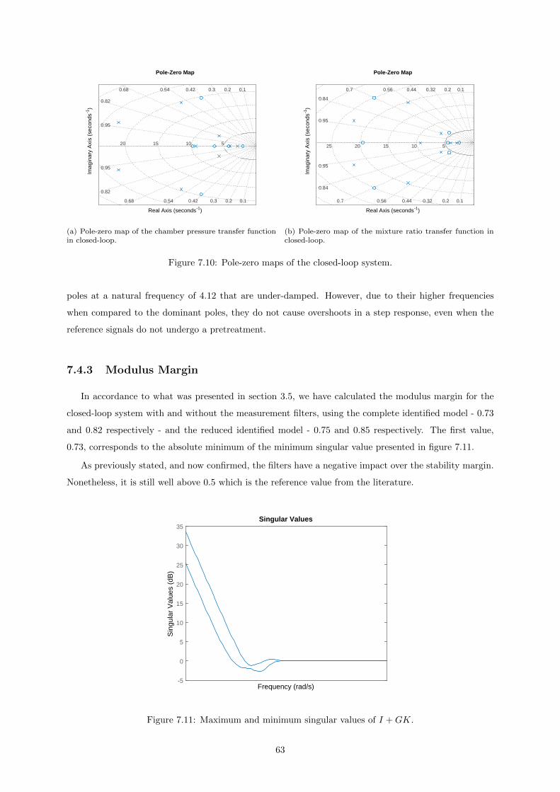
0.1

0.1

0.2

0.2

5

0.3

0.3

0.42

0.42

10

0.54

0.54

15

0.68

0.68

20

0.82

0.95

0.82

0.95

Pole-Zero Map

Real Axis (seconds-1)

Imag

inar

y A

xis

(sec

onds

-1)

(a) Pole-zero map of the chamber pressure transfer functionin closed-loop.

0.1

0.1

0.2

0.2

5

0.32

0.32

10

0.44

0.44

0.56

15

0.56

20

0.7

0.7

25

0.84

0.95

0.84

0.95

Pole-Zero Map

Real Axis (seconds-1)

Imag

inar

y A

xis

(sec

onds

-1)

(b) Pole-zero map of the mixture ratio transfer function inclosed-loop.

Figure 7.10: Pole-zero maps of the closed-loop system.

poles at a natural frequency of 4.12 that are under-damped. However, due to their higher frequencies

when compared to the dominant poles, they do not cause overshoots in a step response, even when the

reference signals do not undergo a pretreatment.

7.4.3 Modulus Margin

In accordance to what was presented in section 3.5, we have calculated the modulus margin for the

closed-loop system with and without the measurement filters, using the complete identified model - 0.73

and 0.82 respectively - and the reduced identified model - 0.75 and 0.85 respectively. The first value,

0.73, corresponds to the absolute minimum of the minimum singular value presented in figure 7.11.

As previously stated, and now confirmed, the filters have a negative impact over the stability margin.

Nonetheless, it is still well above 0.5 which is the reference value from the literature.

-5

0

5

10

15

20

25

30

35Singular Values

Frequency (rad/s)

Sin

gula

r V

alue

s (d

B)

Figure 7.11: Maximum and minimum singular values of I +GK.

63

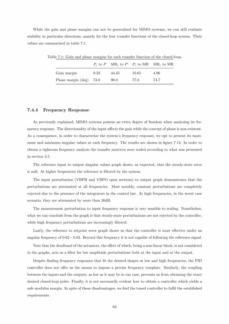
While the gain and phase margins can not be generalized for MIMO systems, we can still evaluate

stability in particular directions, namely for the four transfer functions of the closed-loop system. Their

values are summarized in table 7.1.

Table 7.1: Gain and phase margins for each transfer function of the closed-loop.

Pc to P MRc to P Pc to MR MRc to MR

Gain margin 9.33 44.45 10.65 4.96

Phase margin (deg) 73.0 90.0 77.0 74.7

7.4.4 Frequency Response

As previously explained, MIMO systems possess an extra degree of freedom when analysing its fre-

quency response. The directionality of the input affects the gain while the concept of phase is non-existent.

As a consequence, in order to characterize the system’s frequency response, we opt to present its maxi-

mum and minimum singular values at each frequency. The results are shown in figure 7.12. In order to

obtain a righteous frequency analysis the transfer matrices were scaled according to what was presented

in section 3.5.

The reference input to output singular values graph shows, as expected, that the steady-state error

is null. At higher frequencies the reference is filtered by the system.

The input perturbation (VBPH and VBPO open sections) to output graph demonstrates that the

perturbations are attenuated at all frequencies. Most notably, constant perturbations are completely

rejected due to the presence of the integrators in the control law. At high frequencies, in the worst case

scenario, they are attenuated by more than 20dB.

The measurement perturbation to input frequency response is very sensible to scaling. Nonetheless,

what we can conclude from the graph is that steady-state perturbations are not rejected by the controller,

while high frequency perturbations are increasingly filtered.

Lastly, the reference to setpoint error graph shows us that the controller is most effective under an

angular frequency of 0.62−0.82. Beyond this frequency it is not capable of following the reference signal.

Note that the deadband of the actuators, the effect of which, being a non-linear block, is not considered

in the graphs, acts as a filter for low amplitude perturbations both at the input and at the output.

Despite finding frequency responses that fit the desired shapes at low and high frequencies, the PID

controller does not offer us the means to impose a precise frequency template. Similarly, the coupling

between the inputs and the outputs, as low as it may be in our case, prevents us from obtaining the exact

desired closed-loop poles. Finally, it is not necessarily evident how to obtain a controller which yields a

safe modulus margin. In spite of these disadvantages, we find the tuned controller to fulfil the established

requirements.

64

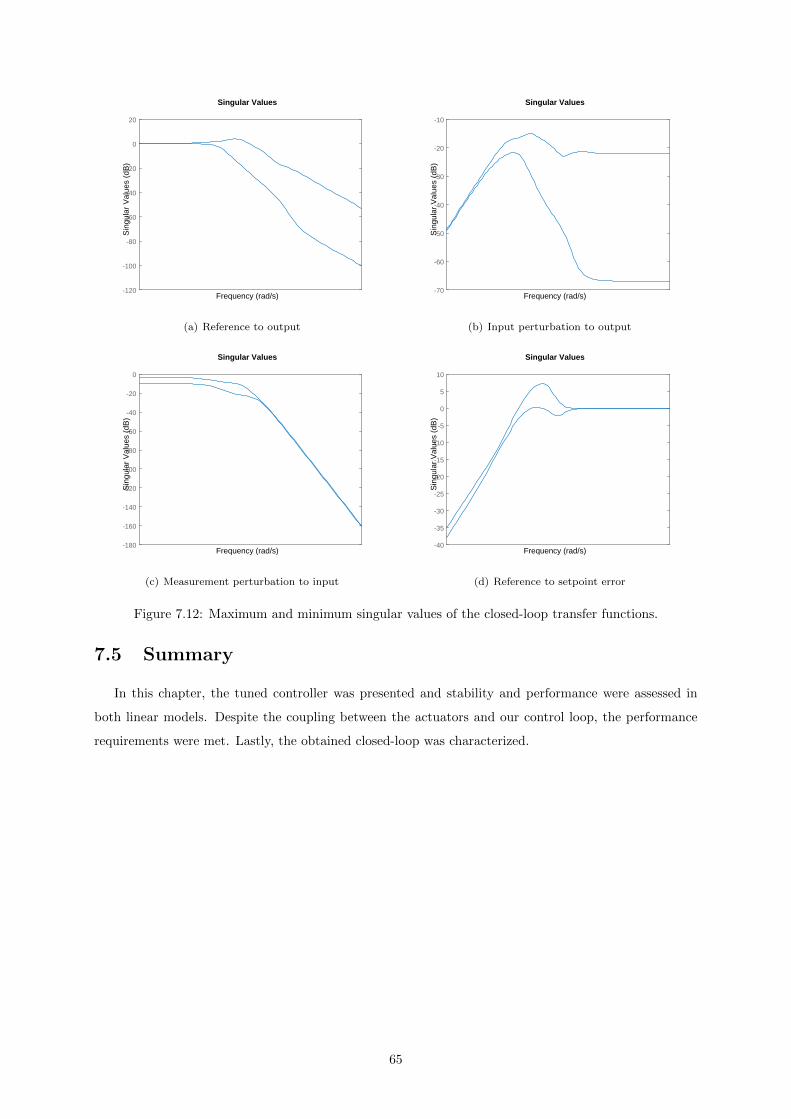
-120

-100

-80

-60

-40

-20

0

20

Singular Values

Frequency (rad/s)

Sin

gula

r V

alue

s (d

B)

(a) Reference to output

-70

-60

-50

-40

-30

-20

-10

Singular Values

Frequency (rad/s)

Sin

gula

r V

alue

s (d

B)

(b) Input perturbation to output

-180

-160

-140

-120

-100

-80

-60

-40

-20

0

Singular Values

Frequency (rad/s)

Sin

gula

r V

alue

s (d

B)

(c) Measurement perturbation to input

-40

-35

-30

-25

-20

-15

-10

-5

0

5

10

Singular Values

Frequency (rad/s)

Sin

gula

r V

alue

s (d

B)

(d) Reference to setpoint error

Figure 7.12: Maximum and minimum singular values of the closed-loop transfer functions.

7.5 Summary

In this chapter, the tuned controller was presented and stability and performance were assessed in

both linear models. Despite the coupling between the actuators and our control loop, the performance

requirements were met. Lastly, the obtained closed-loop was characterized.

65

66

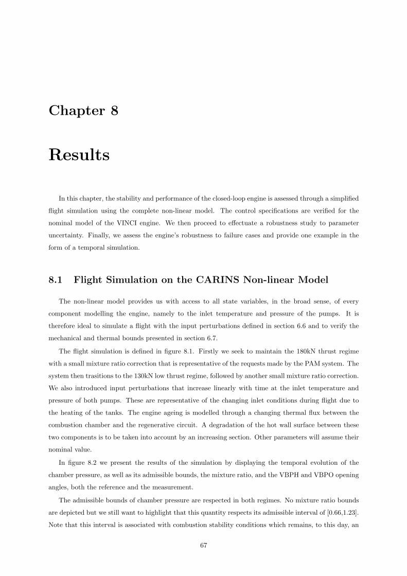
Chapter 8

Results

In this chapter, the stability and performance of the closed-loop engine is assessed through a simplified

flight simulation using the complete non-linear model. The control specifications are verified for the

nominal model of the VINCI engine. We then proceed to effectuate a robustness study to parameter

uncertainty. Finally, we assess the engine’s robustness to failure cases and provide one example in the

form of a temporal simulation.

8.1 Flight Simulation on the CARINS Non-linear Model

The non-linear model provides us with access to all state variables, in the broad sense, of every

component modelling the engine, namely to the inlet temperature and pressure of the pumps. It is

therefore ideal to simulate a flight with the input perturbations defined in section 6.6 and to verify the

mechanical and thermal bounds presented in section 6.7.

The flight simulation is defined in figure 8.1. Firstly we seek to maintain the 180kN thrust regime

with a small mixture ratio correction that is representative of the requests made by the PAM system. The

system then trasitions to the 130kN low thrust regime, followed by another small mixture ratio correction.

We also introduced input perturbations that increase linearly with time at the inlet temperature and

pressure of both pumps. These are representative of the changing inlet conditions during flight due to

the heating of the tanks. The engine ageing is modelled through a changing thermal flux between the

combustion chamber and the regenerative circuit. A degradation of the hot wall surface between these

two components is to be taken into account by an increasing section. Other parameters will assume their

nominal value.

In figure 8.2 we present the results of the simulation by displaying the temporal evolution of the

chamber pressure, as well as its admissible bounds, the mixture ratio, and the VBPH and VBPO opening

angles, both the reference and the measurement.

The admissible bounds of chamber pressure are respected in both regimes. No mixture ratio bounds

are depicted but we still want to highlight that this quantity respects its admissible interval of [0.66,1.23].

Note that this interval is associated with combustion stability conditions which remains, to this day, an

67

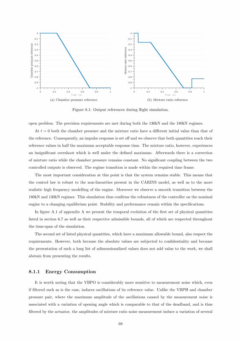
Time (s)0 0.2 0.4 0.6 0.8 1

Cha

mbe

r pr

essu

re r

efer

ence

-1

-0.9

-0.8

-0.7

-0.6

-0.5

-0.4

-0.3

-0.2

-0.1

0

(a) Chamber pressure reference

Time (s)0 0.2 0.4 0.6 0.8 1

Mix

ture

rat

io r

efer

ence

-1

-0.9

-0.8

-0.7

-0.6

-0.5

-0.4

-0.3

-0.2

-0.1

0

(b) Mixture ratio reference

Figure 8.1: Output references during flight simulation.

open problem. The precision requirements are met during both the 130kN and the 180kN regimes.

At t = 0 both the chamber pressure and the mixture ratio have a different initial value than that of

the reference. Consequently, an impulse response is set off and we observe that both quantities reach their

reference values in half the maximum acceptable response time. The mixture ratio, however, experiences

an insignificant overshoot which is well under the defined maximum. Afterwards there is a correction

of mixture ratio while the chamber pressure remains constant. No significant coupling between the two

controlled outputs is observed. The regime transition is made within the required time frame.

The most important consideration at this point is that the system remains stable. This means that

the control law is robust to the non-linearities present in the CARINS model, as well as to the more

realistic high frequency modelling of the engine. Moreover we observe a smooth transition between the

180kN and 130kN regimes. This simulation thus confirms the robustness of the controller on the nominal

engine to a changing equilibrium point. Stability and performance remain within the specifications.

In figure A.1 of appendix A we present the temporal evolution of the first set of physical quantities

listed in section 6.7 as well as their respective admissible bounds, all of which are respected throughout

the time-span of the simulation.

The second set of listed physical quantities, which have a maximum allowable bound, also respect the

requirements. However, both because the absolute values are subjected to confidentiality and because

the presentation of such a long list of adimensionalized values does not add value to the work, we shall

abstain from presenting the results.

8.1.1 Energy Consumption

It is worth noting that the VBPO is considerably more sensitive to measurement noise which, even

if filtered such as is the case, induces oscillations of its reference value. Unlike the VBPH and chamber

pressure pair, where the maximum amplitude of the oscillations caused by the measurement noise is

associated with a variation of opening angle which is comparable to that of the deadband, and is thus

filtered by the actuator, the amplitudes of mixture ratio noise measurement induce a variation of several

68

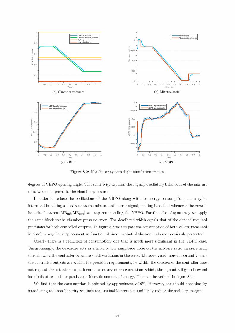
Time0 0.1 0.2 0.3 0.4 0.5 0.6 0.7 0.8 0.9 1

Cha

mbe

r pr

essu

re

0.6

0.7

0.8

0.9

1

Chamber pressureChamber pressure referenceHigh regime boundsLow regime bounds


Time (s)

0 0.1 0.2 0.3 0.4 0.5 0.6 0.7 0.8 0.9 1

Mixture ratio

0.9

0.925

0.95

0.975

1

Mixture ratioMixture ratio reference

(b) Mixture ratio

Time0 0.1 0.2 0.3 0.4 0.5 0.6 0.7 0.8 0.9 1

VB

PH

ope

ning

ang

le

0.75

0.8

0.85

0.9

0.95

1

VBPH angle referenceVBPH opening angle

(c) VBPH

Time0 0.1 0.2 0.3 0.4 0.5 0.6 0.7 0.8 0.9 1

VB

PO

ope

ning

ang

le

0.875

0.9

0.925

0.95

0.975

1

VBPO angle referenceVBPO opening angle

(d) VBPO

Figure 8.2: Non-linear system flight simulation results.

degrees of VBPO opening angle. This sensitivity explains the slightly oscillatory behaviour of the mixture

ratio when compared to the chamber pressure.

In order to reduce the oscillations of the VBPO along with its energy consumption, one may be

interested in adding a deadzone to the mixture ratio error signal, making it so that whenever the error is

bounded between [MRinf,MRsup] we stop commanding the VBPO. For the sake of symmetry we apply

the same block to the chamber pressure error. The deadband width equals that of the defined required

precisions for both controlled outputs. In figure 8.3 we compare the consumption of both valves, measured

in absolute angular displacement in function of time, to that of the nominal case previously presented.

Clearly there is a reduction of consumption, one that is much more significant in the VBPO case.

Unsurprisingly, the deadzone acts as a filter to low amplitude noise on the mixture ratio measurement,

thus allowing the controller to ignore small variations in the error. Moreover, and more importantly, once

the controlled outputs are within the precision requirements, i.e within the deadzone, the controller does

not request the actuators to perform unnecessary micro-corrections which, throughout a flight of several

hundreds of seconds, expend a considerable amount of energy. This can be verified in figure 8.4.

We find that the consumption is reduced by approximately 16%. However, one should note that by

introducing this non-linearity we limit the attainable precision and likely reduce the stability margins.

69

Time0 0.1 0.2 0.3 0.4 0.5 0.6 0.7 0.8 0.9 1

VB

PH

ope

ning

ang

le

0

0.1

0.2

0.3

0.4

0.5

0.6

0.7

0.8

0.9

1

W/o deadzoneW/ Deadzone

(a) VBPH

Time0 0.2 0.4 0.6 0.8 1

VB

PO

ope

ning

ang

le

0

0.1

0.2

0.3

0.4

0.5

0.6

0.7

0.8

0.9

1

W/o deadzoneW/ Deadzone

(b) VBPO

Figure 8.3: Valve consumption comparison when adding a deadzone to the error signals.

Time0 0.1 0.2 0.3 0.4 0.5 0.6 0.7 0.8 0.9 1

Cha

mbe

r pr

essu

re

0.6

0.7

0.8

0.9

1



Time0 0.1 0.2 0.3 0.4 0.5 0.6 0.7 0.8 0.9 1

Mix

ture

rat

io

0.9

0.91

0.92

0.93

0.94

0.95

0.96

0.97

0.98

0.99

1


(b) Mixture ratio

Time0 0.1 0.2 0.3 0.4 0.5 0.6 0.7 0.8 0.9 1

VB

PH

ope

ning

ang

le

0.75

0.8

0.85

0.9

0.95

1


(c) VBPH

Time0 0.1 0.2 0.3 0.4 0.5 0.6 0.7 0.8 0.9 1

VB

PO

ope

ning

ang

le

0.875

0.9

0.925

0.95

0.975

1


(d) VBPO

Figure 8.4: Non-linear system flight simulation results with a dead-band associated to the setpoint error.

70

8.2 Robustness to Parameter Uncertainty

In section 3.6 we mentioned the importance of ensuring that the tuned control law is robust to model

uncertainty, including parametric uncertainty and neglected or unmodelled dynamics. The former is

undoubtedly relevant to our analysis mainly due to component ageing throughout the flight, manufac-

turing tolerances or physical characteristics of the subsystems which are not known with a high degree

of precision. The latter may include non-linearities that evidently are not represented in the linearized

model, unmodelled high frequencies due to the limited scope of the identification method and changing

operating conditions such as when we will transition from the 180kN to the 130kN equilibrium point.

Our validation of the control law will be made in two steps. On the complete linear model we

will simulate flight conditions over a finite set of engine models with varying parameters and operating

conditions. Both stability and performance, which will be quantified hereafter, are to be evaluated over

the uncertainty set.

On the non-linear CARINS model, we have already ensured robustness to the equilibrium point transi-

tion, and guaranteed the stability and performance of the controller in the presence of non-linearities and

more realistic high frequency modelling for the nominal model. The ensemble of the control specifications

listed in section 6 has also been verified for that same model. Hence, in this section we will simulate on

the non-linear model a limited number of the worst cases in terms of stability and performance found

during the linear analysis. Lastly, an upper or lower allowable bound for the failure cases listed in section

6.8 will be determined.

8.2.1 Complete Linear Model

Firstly we define the flight simulation. Figure 8.5 shows the output references of chamber pressure

and mixture ratio with respect to the 180kN equilibrium point. The simulation spans over 1 time unit.

During the initial 0.44 time units we maintain constant chamber pressure but we make a small correction

of mixture ratio at t = 0.27 which is representative of the requests the PAM system will be making during

flight. At t = 0.44 we initiate the equilibrium point transition which lasts precisely 0.11 time units.

Time0 0.2 0.4 0.6 0.8 1

Cha

mbe

r pr

essu

re r

efer

ence

-1

-0.8

-0.6

-0.4

-0.2

0

(a) Chamber pressure reference

Time0 0.2 0.4 0.6 0.8 1

Mix

ture

rat

io r

efer

ence

-1

-0.8

-0.6

-0.4

-0.2

0

(b) Mixture ratio reference

Figure 8.5: Output references during flight simulation.

71

During the simulation we introduce an additive input perturbation which grows linearly over the

simulation time. The final value is 20% of the nominal VBPH and VBPO sections respectively. This

is representative of the slow evolving input perturbations the engine will be subjected to during flight,

namely of inlet temperature and pressure of the pumps.

Stability and performance will be evaluated through several indicators listed below:

1. Modulus margin;

2. Chamber pressure overshoot during the equilibrium point transition;

3. Mixture ratio overshoot during the equilibrium point transition;

4. Maximum difference between the chamber pressure and the chamber pressure reference during the

180kN and 130kN stabilized regimes;

5. Maximum difference between the mixture ratio and the mixture ratio reference during the 180kN

stabilized regime, before and after the step correction, and the 130kN stabilized regime;

6. Chamber pressure and mixture ratio 95% settling time for the equilibrium point transition;

7. Mixture ratio 95% settling time for the correction at t=0.27.

The uncertainty set is required to cover the worst-case scenario which is the engine model for which

our controller renders the closed-loop the closest to instability when compared to the other possible plant

models. Given the extraordinary amount of parameters defining the VINCI engine, we first delved into

identifying, among the uncertain parameters, those for which the system’s dynamics, e.g. the pole-zero

structure and the static gain, are most sensitive to.

The engine ageing is modelled through a changing thermal flux between the combustion chamber and

the regenerative circuit. A degradation of the hot wall surface between these two components is to be

taken into account by a changing interface section Sch.

Other parametric uncertainties with notable effects over the engine’s dynamics include the moments

of inertia of the turbo-pumps (J), the characteristic curves of the hydrogen pump and turbine and the

efficiency of the hydrogen pump (ηH). The hydrogen turbine efficiency is taken into account in its

characteristic curves. The pumps have two characteristic curves describing the pressure output and the

torque. The turbines, on the other hand, also have two characteristic curves but they describe the mass

flow rate and the torque. The uncertainty over the characteristic curves will be modelled through scaling

multiplicative factors EPH, CPH, ETH and CTH respectively. Table 8.1 summarizes the considered

uncertainties. No values can be presented due to confidentiality.

Table 8.1: Studied uncertain parameters.

Parameters JO JH EPH CPH ETH CTH Sch ηH

The uncertainty set includes all of the possible combinations of the bounds of the domains. Its main

disadvantage is that it does not strictly assure us to capture the worst possible configuration for these

72

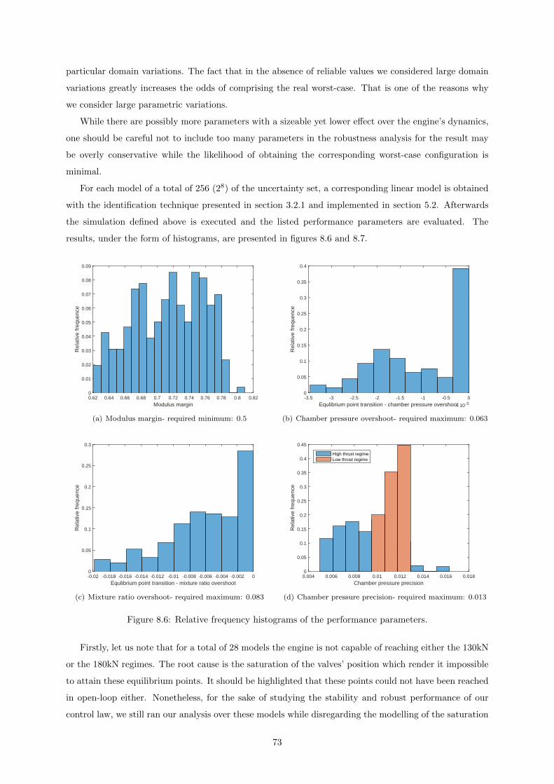
particular domain variations. The fact that in the absence of reliable values we considered large domain

variations greatly increases the odds of comprising the real worst-case. That is one of the reasons why

we consider large parametric variations.

While there are possibly more parameters with a sizeable yet lower effect over the engine’s dynamics,

one should be careful not to include too many parameters in the robustness analysis for the result may

be overly conservative while the likelihood of obtaining the corresponding worst-case configuration is

minimal.

For each model of a total of 256 (28) of the uncertainty set, a corresponding linear model is obtained

with the identification technique presented in section 3.2.1 and implemented in section 5.2. Afterwards

the simulation defined above is executed and the listed performance parameters are evaluated. The

results, under the form of histograms, are presented in figures 8.6 and 8.7.

Modulus margin0.62 0.64 0.66 0.68 0.7 0.72 0.74 0.76 0.78 0.8 0.82

Rel

ativ

e fr

eque

nce

0

0.01

0.02

0.03

0.04

0.05

0.06

0.07

0.08

0.09

(a) Modulus margin- required minimum: 0.5

Equlibrium point transition - chamber pressure overshoot×10-3-3.5 -3 -2.5 -2 -1.5 -1 -0.5 0

Rel

ativ

e fr

eque

nce

0

0.05

0.1

0.15

0.2

0.25

0.3

0.35

0.4

(b) Chamber pressure overshoot- required maximum: 0.063

Equlibrium point transition - mixture ratio overshoot-0.02 -0.018 -0.016 -0.014 -0.012 -0.01 -0.008 -0.006 -0.004 -0.002 0

Rel

ativ

e fr

eque

nce

0

0.05

0.1

0.15

0.2

0.25

0.3

(c) Mixture ratio overshoot- required maximum: 0.083

Chamber pressure precision0.004 0.006 0.008 0.01 0.012 0.014 0.016 0.018

Rel

ativ

e fr

eque

nce

0

0.05

0.1

0.15

0.2

0.25

0.3

0.35

0.4

0.45

High thrust regimeLow thrust regime

(d) Chamber pressure precision- required maximum: 0.013

Figure 8.6: Relative frequency histograms of the performance parameters.

Firstly, let us note that for a total of 28 models the engine is not capable of reaching either the 130kN

or the 180kN regimes. The root cause is the saturation of the valves’ position which render it impossible

to attain these equilibrium points. It should be highlighted that these points could not have been reached

in open-loop either. Nonetheless, for the sake of studying the stability and robust performance of our

control law, we still ran our analysis over these models while disregarding the modelling of the saturation

73

Mixture ratio precision0.006 0.008 0.01 0.012 0.014 0.016 0.018 0.02

Rel

ativ

e fr

eque

nce

0

0.05

0.1

0.15

0.2

0.25

0.3

High thrust regimeLow thrust regime

(a) Mixture ratio precision- required maximum: 0.033

Equilibrium point transition - chamber pressure settling time0.1095 0.11 0.1105 0.111 0.1115 0.112 0.1125 0.113

Rel

ativ

e fr

eque

nce

0

0.05

0.1

0.15

0.2

0.25

(b) Chamber pressure settling time- reference value: 0.1096

Equilibrium point transition - mixture ratio settling time0.104 0.105 0.106 0.107 0.108 0.109 0.11 0.111 0.112

Rel

ativ

e fr

eque

nce

0

0.05

0.1

0.15

0.2

0.25

0.3

(c) Mixture ratio settling time- reference value: 0.1096

Mixture ratio correction settling time0.01 0.012 0.014 0.016 0.018 0.02 0.022 0.024 0.026 0.028

Rel

ativ

e fr

eque

nce

0

0.1

0.2

0.3

0.4

0.5

0.6

0.7

(d) Mixture ratio correction settling time- required maxi-mum: 0.028

Figure 8.7: Relative frequency histograms of the performance parameters.

of the valves. Our conclusions about the control law are valid even though in reality the engine can

not handle these extreme cases. Both because the project is still in an early phase and because we use

very conservative data about the uncertainties, we will refrain from trying to quantify the probability

of having said cases. Moreover we point out that the modelling of the valves is not final, namely the

relationship between the open angle and the open section. Further information about the modelling of

the VINCI engine may be made available in the near future as well.

The modulus margin is consistently higher than 0.5 which is our reference value from the literature.

Chamber pressure and mixture ratio overshoots are well below the maximum acceptable values. Regarding

the precision, there are only a handful of cases in which the chamber pressure limit is significantly

surpassed. Let us note however that these are singular events, the duration of which is meaningless

throughout the course of the boosted flight. These are therefore acceptable. The mixture ratio, on the

other hand, is kept at all times below the target value. Lastly, the settling times, either for regime

transition or for a correction of mixture ratio, are well within the requirements. While 0.1096 was our

target time for transition, that is also the time the reference values take to reach the 130kN equilibrium

point. Consequently the settling times of both outputs are often higher than this value, to a maximum

74

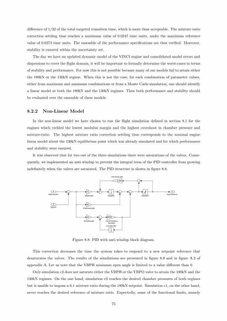
difference of 1/32 of the total targeted transition time, which is more than acceptable. The mixture ratio

correction settling time reaches a maximum value of 0.0247 time units, under the maximum reference

value of 0.0274 time units. The ensemble of the performance specifications are thus verified. Moreover,

stability is ensured within the uncertainty set.

The day we have an updated dynamic model of the VINCI engine and consolidated model errors and

dispersions to cover the flight domain, it will be important to formally determine the worst-cases in terms

of stability and performance. For now this is not possible because many of our models fail to attain either

the 180kN or the 130kN regime. When this is not the case, for each combination of parameter values,

either from maximum and minimum combinations or from a Monte Carlo simulation, one should identify

a linear model at both the 180kN and the 130kN regimes. Then both performance and stability should

be evaluated over the ensemble of these models.

8.2.2 Non-Linear Model

In the non-linear model we have chosen to run the flight simulation defined in section 8.1 for the

engines which yielded the lowest modulus margin and the highest overshoot in chamber pressure and

mixture-ratio. The highest mixture ratio correction settling time corresponds to the nominal engine

linear model about the 130kN equilibrium point which was already simulated and for which performance

and stability were ensured.

It was observed that for two out of the three simulations there were saturations of the valves. Conse-

quently, we implemented an anti-windup to prevent the integral term of the PID controller from growing

indefinitely when the valves are saturated. The PID structure is shown in figure 8.8.

1

Measurement

1

Input reference

1s

Integrator

2

Setpoint

ki

Integral gain

kp

Proportional gain

kd

Derivative gain

Saturation

Nfilter

Cut-off frequency

Derivative

1s

Low-pass filter

k_awu

Anti-windup gain

Figure 8.8: PID with anti-windup block diagram.

This correction decreases the time the system takes to respond to a new setpoint reference that

desaturates the valves. The results of the simulations are presented in figure 8.9 and in figure A.2 of

appendix A. Let us note that the VBPH minimum open angle is limited to a value different than 0.

Only simulation c3 does not saturate either the VBPH or the VBPO valve to attain the 180kN and the

130kN regimes. On the one hand, simulation c2 reaches the desired chamber pressures of both regimes

but is unable to impose a 6.1 mixture ratio during the 180kN setpoint. Simulation c1, on the other hand,

never reaches the desired reference of mixture ratio. Expectedly, some of the functional limits, namely

75

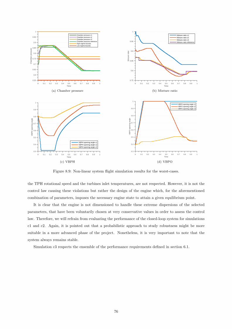
Time0 0.1 0.2 0.3 0.4 0.5 0.6 0.7 0.8 0.9 1

Cha

mbe

r pr

essu

re

0.55

0.6

0.65

0.7

0.75

0.8

0.85

0.9

0.95

1

Chamber pressure c1Chamber pressure c2Chamber pressure c3Chamber pressure referenceHigh regime boundsLow regime bounds


Time0 0.1 0.2 0.3 0.4 0.5 0.6 0.7 0.8 0.9 1

Mix

ture

rat

io

0.75

0.8

0.85

0.9

0.95

1

Mixture ratio c1Mixture ratio c2Mixture ratio c3Mixture ratio reference

(b) Mixture ratio

Time0 0.1 0.2 0.3 0.4 0.5 0.6 0.7 0.8 0.9 1

VB

PH

ope

ning

ang

le

0.3

0.4

0.5

0.6

0.7

0.8

0.9

1

VBPH opening angle c1VBPH opening angle c2VBPH opening angle c3

(c) VBPH

Time0 0.1 0.2 0.3 0.4 0.5 0.6 0.7 0.8 0.9 1

VB

PO

ope

ning

ang

le

0.3

0.4

0.5

0.6

0.7

0.8

0.9

1

VBPO opening angle c1VBPO opening angle c2VBPO opening angle c3

(d) VBPO

Figure 8.9: Non-linear system flight simulation results for the worst-cases.

the TPH rotational speed and the turbines inlet temperatures, are not respected. However, it is not the

control law causing these violations but rather the design of the engine which, for the aforementioned

combination of parameters, imposes the necessary engine state to attain a given equilibrium point.

It is clear that the engine is not dimensioned to handle these extreme dispersions of the selected

parameters, that have been voluntarily chosen at very conservative values in order to assess the control

law. Therefore, we will refrain from evaluating the performance of the closed-loop system for simulations

c1 and c2. Again, it is pointed out that a probabilistic approach to study robustness might be more

suitable in a more advanced phase of the project. Nonetheless, it is very important to note that the

system always remains stable.

Simulation c3 respects the ensemble of the performance requirements defined in section 6.1.

76

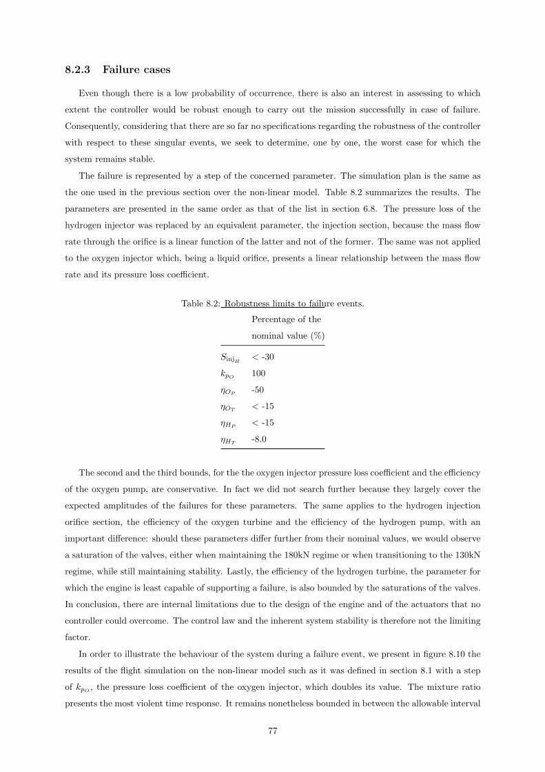
8.2.3 Failure cases

Even though there is a low probability of occurrence, there is also an interest in assessing to which

extent the controller would be robust enough to carry out the mission successfully in case of failure.

Consequently, considering that there are so far no specifications regarding the robustness of the controller

with respect to these singular events, we seek to determine, one by one, the worst case for which the

system remains stable.

The failure is represented by a step of the concerned parameter. The simulation plan is the same as

the one used in the previous section over the non-linear model. Table 8.2 summarizes the results. The

parameters are presented in the same order as that of the list in section 6.8. The pressure loss of the

hydrogen injector was replaced by an equivalent parameter, the injection section, because the mass flow

rate through the orifice is a linear function of the latter and not of the former. The same was not applied

to the oxygen injector which, being a liquid orifice, presents a linear relationship between the mass flow

rate and its pressure loss coefficient.

Table 8.2: Robustness limits to failure events.

Percentage of the

nominal value (%)

SinjH < -30

kpO 100

ηOP -50

ηOT < -15

ηHP < -15

ηHT -8.0

The second and the third bounds, for the the oxygen injector pressure loss coefficient and the efficiency

of the oxygen pump, are conservative. In fact we did not search further because they largely cover the

expected amplitudes of the failures for these parameters. The same applies to the hydrogen injection

orifice section, the efficiency of the oxygen turbine and the efficiency of the hydrogen pump, with an

important difference: should these parameters differ further from their nominal values, we would observe

a saturation of the valves, either when maintaining the 180kN regime or when transitioning to the 130kN

regime, while still maintaining stability. Lastly, the efficiency of the hydrogen turbine, the parameter for

which the engine is least capable of supporting a failure, is also bounded by the saturations of the valves.

In conclusion, there are internal limitations due to the design of the engine and of the actuators that no

controller could overcome. The control law and the inherent system stability is therefore not the limiting

factor.

In order to illustrate the behaviour of the system during a failure event, we present in figure 8.10 the

results of the flight simulation on the non-linear model such as it was defined in section 8.1 with a step

of kpO , the pressure loss coefficient of the oxygen injector, which doubles its value. The mixture ratio

presents the most violent time response. It remains nonetheless bounded in between the allowable interval

77

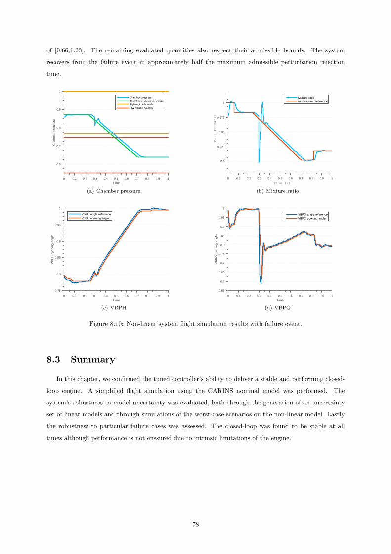
of [0.66,1.23]. The remaining evaluated quantities also respect their admissible bounds. The system

recovers from the failure event in approximately half the maximum admissible perturbation rejection

time.

Time0 0.1 0.2 0.3 0.4 0.5 0.6 0.7 0.8 0.9 1

Cha

mbe

r pr

essu

re

0.6

0.7

0.8

0.9

1



Time (s)

0 0.1 0.2 0.3 0.4 0.5 0.6 0.7 0.8 0.9 1

Mixture ratio

0.9

0.925

0.95

0.975

1


(b) Mixture ratio

Time0 0.1 0.2 0.3 0.4 0.5 0.6 0.7 0.8 0.9 1

VB

PH

ope

ning

ang

le

0.75

0.8

0.85

0.9

0.95

1


(c) VBPH

Time0 0.1 0.2 0.3 0.4 0.5 0.6 0.7 0.8 0.9 1

VB

PO

ope

ning

ang

le

0.55

0.6

0.65

0.7

0.75

0.8

0.85

0.9

0.95

1


(d) VBPO

Figure 8.10: Non-linear system flight simulation results with failure event.

8.3 Summary

In this chapter, we confirmed the tuned controller’s ability to deliver a stable and performing closed-

loop engine. A simplified flight simulation using the CARINS nominal model was performed. The

system’s robustness to model uncertainty was evaluated, both through the generation of an uncertainty

set of linear models and through simulations of the worst-case scenarios on the non-linear model. Lastly

the robustness to particular failure cases was assessed. The closed-loop was found to be stable at all

times although performance is not enssured due to intrinsic limitations of the engine.

78

Chapter 9

Conclusion and Future Work

9.1 Conclusion

The main focus of this thesis was to define, analyse and solve a control problem, one in which the

controlled quantities are the thrust and mixture ratio of a liquid bi-propellant rocket engine. Motivated

mainly by the necessity of improving the performances of current European launchers, a methodology

to, firstly, model and analyse the dynamics of a rocket engine, and secondly, to design and validate an

appropriate control law, was established. Our numerical application was the VINCI rocket engine which

is meant to equip the second stage of Ariane 6.

Firstly an analytic linear model in the state-space form was sought out. A comparison between

this model, issued from the linearization of the governing equations of the engine, and the non-linear

model, previously developed in-house, was drawn. The results not being satisfactory, the least-squares

identification method was used in order to obtain a physical, both complete and reduced, linear model of

the engine. Notably, both the complete and the reduced state vectors were deduced based on the analytic

analysis. After validating the identified models, a sensitivity analysis over a limited number of design

parameters was effectuated. It was concluded that the regenerative circuit is mostly responsible for the

slowest mode, although it is not observable/controllable, and that the turbo-pumps are closely related to

the dominant modes which determine the settling times of the step-response.

Secondly a double-PID controller was designed using SISO design techniques. The effects of both the

valves and the sensors were evaluated and mitigated by readjusting the controller and implementing a

feed-forward. After validating the solution on the reduced and complete linear models, the closed-loop

was characterized, namely by calculating the modulus margin, the closed-loop poles and the frequency

response. On the non-linear CARINS model, we validated the controller by ensuring stability and perfor-

mance in presence of non-linearities, of a changing operating point and of an overall more realistic model.

The ensemble of the control specifications were verified on the nominal model.

Lastly, the robustness of the controller was tested against parametric uncertainties. A large number

of perturbed linear models was generated and the performances during a flight simulation were presented

in a statistical fashion. A similar flight simulation was run on the nominal non-linear model, for which

79

stability, performance and the functional bounds of the engine components were verified against what

was defined as the target values at the beginning of the project. The system’s tolerance to singular failure

events was also determined.

The main achievement of this thesis, and its first listed objective, was obtaining a low order physical

linear model of the engine, specifically one that can be used to design control laws. As a consequence, the

components and the uncertainties which play a major role in the dynamics of the engine were identified.

Moreover, it was demonstrated that a modified PID controller is sufficient to control the engine. While

a more rigorous robustness analysis is needed as soon as more information about the engine is made

available, it was still observed that the engine controller is robust to very conservative uncertainties and

that the engine will sooner saturate due to its own design than the control law will render the system

unstable.

9.2 Future Work

There are several aspects of the developed work that warrant further investigation. Firstly, the

analytic approach to obtain a linear-model, which for several reasons failed to provide a fitting time-

response, should be employed in a different engine in order to better comprehend the reasons for its

misrepresentation. Moreover, the engine sensitivity analysis, which was effectuated solely for four different

parameters, could be extended to other parameters of interest.

As soon as more detailed information about the valves’ dynamic model, the sensors, the parametric

uncertainties and the functional limits of the components is made available, a more rigorous robustness

analysis ought to be held. Specifically, we could opt to run a Monte Carlo simulation over the non-linear

model or to use the µ analysis framework if we are successful in obtaining a fitting analytic model. In

function of the results, new approaches to design the controller may be put in place, for instance the

structured H-infinity coupled with a PID control structure. In order to fully validate the control law it is

also mandatory to design a mixture-ratio estimator and evaluate its impact on the overall performance

and stability of the closed-loop system.

Lastly, the application of the same methodology to other engines should be considered. While the

VINCI engine was found to be a rather simple control problem, with relaxed constraints, it may not

be the case when studying other thermodynamic cycles, namely the gas-generator cycle of the Vulcain

rocket engine.

80

Bibliography

[1] D. A. Shearer and G. L. Vogt. Rockets - an educator’s guide with ac-

tivities in science, mathematics, and technology, 2003. Retrieved from:

http://quest.arc.nasa.gov/space/teachers/rockets/58269main Rockets.Guide.pdf.

[2] G. P. Sutton and O. Biblarz. Rocket Propulsion Elements, chapter 2-4. John Wiley and Sons, 2001.

[3] J. H. Wyld. Fundamental equations of rocket motion: Part i - flight in airless space. Astronautics,

Vol. 6(No. 35):pp. 13–16, 1936.

[4] E. Y. Choueiri. A critical history of electric propulsion: The first 50 years (1906-1956). Journal of

Propulsion and Power 20.2, pages pp. 193–203, 2004.

[5] B. Ward. Space: The Life of Wernher von Braun. Naval Institute Press, 2013.

[6] M. J. Casiano, J. R. Hulka, and V. Yang. Liquid-propellant rocket engine throttling: A comprehen-

sive review. Journal of Propulsion and Power, 2010.

[7] E. M. Betts and R. A. Frederick. A historical systems study of liquid rocket engine throttling ca-

pabilities. 46th AIAA/ASME/SAE/ASEE Joint Propulsion Conference & Exhibit, Joint Propulsion

Conferences, 2010.

[8] S.L Harris. Block ii: The new space shuttle main engine. 32nd Joint Propulsion Conference and

Exhibit, Joint Propulsion Conferences, 1996.

[9] SpaceX. Falcon 9 Launch Vehicle - PAYLOAD USER’S GUIDE, rev 2 edition, October 2015.

[10] A. Santana, F.I. Barbosa, M. Niwa, and L.C.S. Goes. Modeling and robust analysis of a liquid rocket

engine. American Institute of Aeronautics and Astronautics, 2000.

[11] A. Allahverdizadeh and B. Dadashzadeh. A fuzzy logic controller for thrust level control of liquid

propellant engines. Scientific Cooperations International Workshops on Electrical and Computer

Engineering Subfields, 2014.

[12] A. Duyar and T. Guo. Space shuttle main engine model identification. IEEE Control Systems

Magazine, 1990.

[13] A. Duyar, V. Eldem, W. C. Merril, and T. Guo. Space shuttle main engine model identification.

Journal of Dynamic Systems, Measurement, and Control, 1989.

81

[14] A. Nassirharand and H. Karimi. Controller synthesis methodology for multivariable nonlinear sys-

tems with application to aerospace. Journal of Dynamic Systems, Measurement, and Control, 2004.

[15] H. Sunakawa, A. Kurosu, K. Okita, W. Sakai, S. Maeda, and A. Ogawara. Automatic thrust and

mixture ratio control of the LE-X. 44th AIAA/ASME/SAE/ASEE Joint Propulsion Conference and

Exhibit, 2008.

[16] A. Nassirharand and H. Karimi. Mixture ratio control of liquid propellant engines. Aircraf Engi-

neering and Aerospace Technology: An International Journal, 2005.

[17] A. Ray, M.S. Holmes, and C.F. Lorenzo. Nonlinear control of a reusable rocket engine for life

extension. American Control Conference, 1998.

[18] A. Ray M.S. Holmes and C.F. Lorenzo. Life extending controller design for reusable rocket engines.

The Aeronautical Journal, 2001.

[19] D. K. Huzel and D. H. Huang. Modern Engineering for Design of Liquid-Propellant Rocket Engines,

chapter 1,2,5,6. American Institute of Aeronautics and Astronautics, 1992.

[20] C. L. Lawson and R. J. Hanson. Solving Least squares problems. Society for Industrial and Applied

Mathematics, 1987.

[21] S. Skogestad and I. Postlethwaite. Multivariable Feedback Control: Analysis and Design, chapter

2-4,7,Appendix A. John Wiley and Sons, 2005.

[22] S. J. Miller. The method of least squares. Mathematics Department Brown University, pages 1–7,

2006.

[23] K. Willcox and J. Peraire. Balanced model reduction via the proper orthogonal decomposition.

AIAA journal 40.11: 2323-2330, 2002.

[24] Snecma. Propulsion spatiale - vinci, 2011. Retrieved from: http://www.safran-aircraft-

engines.com/fr/file/download/fiche vinci 2011 hd.pdf.

82

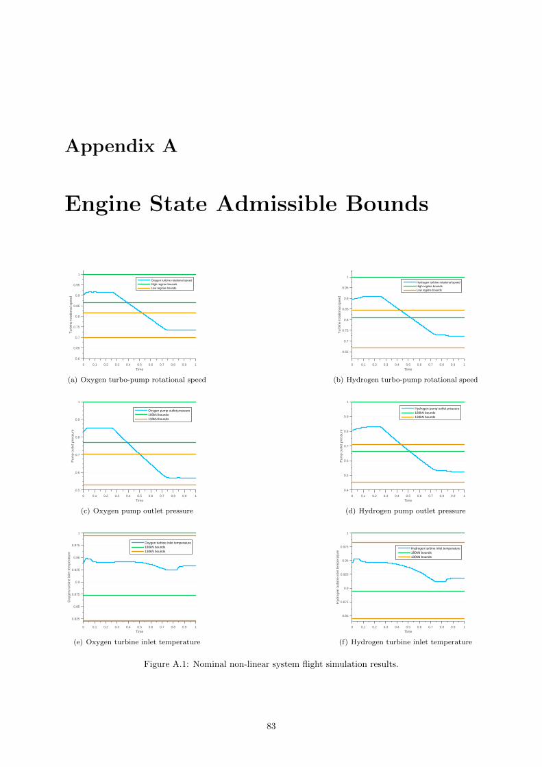
Appendix A

Engine State Admissible Bounds

Time0 0.1 0.2 0.3 0.4 0.5 0.6 0.7 0.8 0.9 1

Tur

bine

rot

atio

nal s

peed

0.6

0.65

0.7

0.75

0.8

0.85

0.9

0.95

1

Oxygen turbine rotational speedHigh regime boundsLow regime bounds

(a) Oxygen turbo-pump rotational speed

Time0 0.1 0.2 0.3 0.4 0.5 0.6 0.7 0.8 0.9 1

Tur

bine

rot

atio

nal s

peed

0.65

0.7

0.75

0.8

0.85

0.9

0.95

1

Hydrogen turbine rotational speedHigh regime boundsLow regime bounds

(b) Hydrogen turbo-pump rotational speed

Time0 0.1 0.2 0.3 0.4 0.5 0.6 0.7 0.8 0.9 1

Pum

p ou

tlet p

ress

ure

0.5

0.6

0.7

0.8

0.9

1

Oxygen pump outlet pressure180kN bounds130kN bounds

(c) Oxygen pump outlet pressure

Time0 0.1 0.2 0.3 0.4 0.5 0.6 0.7 0.8 0.9 1

Pum

p ou

tlet p

ress

ure

0.4

0.5

0.6

0.7

0.8

0.9

1

Hydrogen pump outlet pressure180kN bounds130kN bounds

(d) Hydrogen pump outlet pressure

Time0 0.1 0.2 0.3 0.4 0.5 0.6 0.7 0.8 0.9 1

Oxy

gen

turb

ine

inle

t tem

pera

ture

0.825

0.85

0.875

0.9

0.925

0.95

0.975

1

Oxygen turbine inlet temperature180kN bounds130kN bounds

(e) Oxygen turbine inlet temperature

Time0 0.1 0.2 0.3 0.4 0.5 0.6 0.7 0.8 0.9 1

Hyd

roge

n tu

rbin

e in

let t

empe

ratu

re

0.85

0.875

0.9

0.925

0.95

0.975

1

Hydrogen turbine inlet temperature180kN bounds130kN bounds

(f) Hydrogen turbine inlet temperature

Figure A.1: Nominal non-linear system flight simulation results.

83

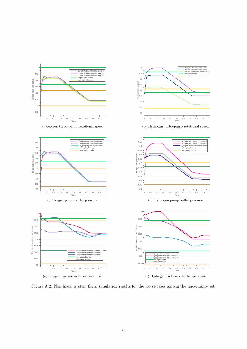
Time0 0.1 0.2 0.3 0.4 0.5 0.6 0.7 0.8 0.9 1

Tur

bine

rot

atio

nal s

peed

0.65

0.7

0.75

0.8

0.85

0.9

0.95

1

Oxygen turbine rotational speed c1Oxygen turbine rotational speed c2Oxygen turbine rotational speed c3High regime boundsLow regime bounds

(a) Oxygen turbo-pump rotational speed

Time0 0.1 0.2 0.3 0.4 0.5 0.6 0.7 0.8 0.9

Tur

bine

rot

atio

nal s

peed

0.6

0.65

0.7

0.75

0.8

0.85

0.9

0.95

1 Hydrogen turbine rotational speed c1Hydrogen turbine rotational speed c2Hydrogen turbine rotational speed c3High regime boundsLow regime bounds

(b) Hydrogen turbo-pump rotational speed

Time0 0.1 0.2 0.3 0.4 0.5 0.6 0.7 0.8 0.9 1

Pum

p ou

tlet p

ress

ure

0.5

0.55

0.6

0.65

0.7

0.75

0.8

0.85

0.9

0.95

1

Oxygen pump outlet pressure c1Oxygen pump outlet pressure c2Oxygen pump outlet pressure c3High regime boundsLow regime bounds

(c) Oxygen pump outlet pressure

Time0 0.1 0.2 0.3 0.4 0.5 0.6 0.7 0.8 0.9 1

Pum

p ou

tlet p

ress

ure

0.4

0.45

0.5

0.55

0.6

0.65

0.7

0.75

0.8

0.85

0.9

0.95

1

Hydrogen pump outlet pressure c1Hydrogen pump outlet pressure c2Hydrogen pump outlet pressure c3High regime boundsLow regime bounds

(d) Hydrogen pump outlet pressure

Time0 0.1 0.2 0.3 0.4 0.5 0.6 0.7 0.8 0.9 1

Oxy

gen

turb

ine

inle

t tem

pera

ture

0.8

0.825

0.85

0.875

0.9

0.925

0.95

0.975

1

Oxygen turbine inlet temperature c1Oxygen turbine inlet temperature c2Oxygen turbine inlet temperature c3High regime boundsLow regime bounds

(e) Oxygen turbine inlet temperature

Time0 0.1 0.2 0.3 0.4 0.5 0.6 0.7 0.8 0.9 1

Hyd

roge

n tu

rbin

e in

let t

empe

ratu

re

0.825

0.85

0.875

0.9

0.925

0.95

0.975

1

Hydrogen turbine inlet temperature c1Hydrogen turbine inlet temperature c2Hydrogen turbine inlet temperature c3High regime boundsLow regime bounds

(f) Hydrogen turbine inlet temperature

Figure A.2: Non-linear system flight simulation results for the worst-cases among the uncertainty set.

84

Documents

Mixture Ratio and Thrust Control of a Liquid-Propellant ... · PDF fileMixture Ratio and Thrust Control of a Liquid-Propellant ... 1.1.1 Controlled Engines and Reusable Rockets