Mixture Models and EM - Penn State College of …rtc12/CSE586Spring2010/papers/prmlMixturesEM.pdf · Mixture Models and EM ... Gaussian mixture models are widely used in data mining,

9Mixture Models

and EM

If we define a joint distribution over observed and latent variables, the correspond-ing distribution of the observed variables alone is obtained by marginalization. Thisallows relatively complex marginal distributions over observed variables to be ex-pressed in terms of more tractable joint distributions over the expanded space ofobserved and latent variables. The introduction of latent variables thereby allowscomplicated distributions to be formed from simpler components. In this chapter,we shall see that mixture distributions, such as the Gaussian mixture discussed inSection 2.3.9, can be interpreted in terms of discrete latent variables. Continuouslatent variables will form the subject of Chapter 12.

As well as providing a framework for building more complex probability dis-tributions, mixture models can also be used to cluster data. We therefore begin ourdiscussion of mixture distributions by considering the problem of finding clustersin a set of data points, which we approach first using a nonprobabilistic techniquecalled the K-means algorithm (Lloyd, 1982). Then we introduce the latent variableSection 9.1

423

424 9. MIXTURE MODELS AND EM

view of mixture distributions in which the discrete latent variables can be interpretedas defining assignments of data points to specific components of the mixture. A gen-Section 9.2eral technique for finding maximum likelihood estimators in latent variable modelsis the expectation-maximization (EM) algorithm. We first of all use the Gaussianmixture distribution to motivate the EM algorithm in a fairly informal way, and thenwe give a more careful treatment based on the latent variable viewpoint. We shallSection 9.3see that the K-means algorithm corresponds to a particular nonprobabilistic limit ofEM applied to mixtures of Gaussians. Finally, we discuss EM in some generality.Section 9.4

Gaussian mixture models are widely used in data mining, pattern recognition,machine learning, and statistical analysis. In many applications, their parameters aredetermined by maximum likelihood, typically using the EM algorithm. However, aswe shall see there are some significant limitations to the maximum likelihood ap-proach, and in Chapter 10 we shall show that an elegant Bayesian treatment can begiven using the framework of variational inference. This requires little additionalcomputation compared with EM, and it resolves the principal difficulties of maxi-mum likelihood while also allowing the number of components in the mixture to beinferred automatically from the data.

9.1. K-means Clustering

We begin by considering the problem of identifying groups, or clusters, of data pointsin a multidimensional space. Suppose we have a data set {x1, . . . ,xN} consistingof N observations of a random D-dimensional Euclidean variable x. Our goal is topartition the data set into some number K of clusters, where we shall suppose forthe moment that the value of K is given. Intuitively, we might think of a cluster ascomprising a group of data points whose inter-point distances are small comparedwith the distances to points outside of the cluster. We can formalize this notion byfirst introducing a set of D-dimensional vectors µk, where k = 1, . . . , K, in whichµk is a prototype associated with the kth cluster. As we shall see shortly, we canthink of the µk as representing the centres of the clusters. Our goal is then to findan assignment of data points to clusters, as well as a set of vectors {µk}, such thatthe sum of the squares of the distances of each data point to its closest vector µk, isa minimum.

It is convenient at this point to define some notation to describe the assignmentof data points to clusters. For each data point xn, we introduce a corresponding setof binary indicator variables rnk ∈ {0, 1}, where k = 1, . . . , K describing which ofthe K clusters the data point xn is assigned to, so that if data point xn is assigned tocluster k then rnk = 1, and rnj = 0 for j = k. This is known as the 1-of-K codingscheme. We can then define an objective function, sometimes called a distortionmeasure, given by

J =N∑

n=1

K∑k=1

rnk‖xn − µk‖2 (9.1)

which represents the sum of the squares of the distances of each data point to its

9.1. K-means Clustering 425

assigned vector µk. Our goal is to find values for the {rnk} and the {µk} so as tominimize J . We can do this through an iterative procedure in which each iterationinvolves two successive steps corresponding to successive optimizations with respectto the rnk and the µk. First we choose some initial values for the µk. Then in the firstphase we minimize J with respect to the rnk, keeping the µk fixed. In the secondphase we minimize J with respect to the µk, keeping rnk fixed. This two-stageoptimization is then repeated until convergence. We shall see that these two stagesof updating rnk and updating µk correspond respectively to the E (expectation) andM (maximization) steps of the EM algorithm, and to emphasize this we shall use theSection 9.4terms E step and M step in the context of the K-means algorithm.

Consider first the determination of the rnk. Because J in (9.1) is a linear func-tion of rnk, this optimization can be performed easily to give a closed form solution.The terms involving different n are independent and so we can optimize for eachn separately by choosing rnk to be 1 for whichever value of k gives the minimumvalue of ‖xn − µk‖2. In other words, we simply assign the nth data point to theclosest cluster centre. More formally, this can be expressed as

rnk ={

1 if k = arg minj ‖xn − µj‖2

0 otherwise.(9.2)

Now consider the optimization of the µk with the rnk held fixed. The objectivefunction J is a quadratic function of µk, and it can be minimized by setting itsderivative with respect to µk to zero giving

2N∑

n=1

rnk(xn − µk) = 0 (9.3)

which we can easily solve for µk to give

µk =∑

n rnkxn∑n rnk

. (9.4)

The denominator in this expression is equal to the number of points assigned tocluster k, and so this result has a simple interpretation, namely set µk equal to themean of all of the data points xn assigned to cluster k. For this reason, the procedureis known as the K-means algorithm.

The two phases of re-assigning data points to clusters and re-computing the clus-ter means are repeated in turn until there is no further change in the assignments (oruntil some maximum number of iterations is exceeded). Because each phase reducesthe value of the objective function J , convergence of the algorithm is assured. How-Exercise 9.1ever, it may converge to a local rather than global minimum of J . The convergenceproperties of the K-means algorithm were studied by MacQueen (1967).

The K-means algorithm is illustrated using the Old Faithful data set in Fig-Appendix Aure 9.1. For the purposes of this example, we have made a linear re-scaling of thedata, known as standardizing, such that each of the variables has zero mean andunit standard deviation. For this example, we have chosen K = 2, and so in this


(a)

−2 0 2

−2

0

2 (b)

−2 0 2

−2

0

2 (c)

−2 0 2

−2

0

2

(d)

−2 0 2

−2

0

2 (e)

−2 0 2

−2

0

2 (f)

−2 0 2

−2

0

2

(g)

−2 0 2

−2

0

2 (h)

−2 0 2

−2

0

2 (i)

−2 0 2

−2

0

2

Figure 9.1 Illustration of the K-means algorithm using the re-scaled Old Faithful data set. (a) Green pointsdenote the data set in a two-dimensional Euclidean space. The initial choices for centres µ1 and µ2 are shownby the red and blue crosses, respectively. (b) In the initial E step, each data point is assigned either to the redcluster or to the blue cluster, according to which cluster centre is nearer. This is equivalent to classifying thepoints according to which side of the perpendicular bisector of the two cluster centres, shown by the magentaline, they lie on. (c) In the subsequent M step, each cluster centre is re-computed to be the mean of the pointsassigned to the corresponding cluster. (d)–(i) show successive E and M steps through to final convergence ofthe algorithm.


Figure 9.2 Plot of the cost function J given by(9.1) after each E step (blue points)and M step (red points) of the K-means algorithm for the exampleshown in Figure 9.1. The algo-rithm has converged after the thirdM step, and the final EM cycle pro-duces no changes in either the as-signments or the prototype vectors.

J

1 2 3 40

500

1000

case, the assignment of each data point to the nearest cluster centre is equivalent to aclassification of the data points according to which side they lie of the perpendicularbisector of the two cluster centres. A plot of the cost function J given by (9.1) forthe Old Faithful example is shown in Figure 9.2.

Note that we have deliberately chosen poor initial values for the cluster centresso that the algorithm takes several steps before convergence. In practice, a betterinitialization procedure would be to choose the cluster centres µk to be equal to arandom subset of K data points. It is also worth noting that the K-means algorithmitself is often used to initialize the parameters in a Gaussian mixture model beforeapplying the EM algorithm.Section 9.2.2

A direct implementation of the K-means algorithm as discussed here can berelatively slow, because in each E step it is necessary to compute the Euclidean dis-tance between every prototype vector and every data point. Various schemes havebeen proposed for speeding up the K-means algorithm, some of which are based onprecomputing a data structure such as a tree such that nearby points are in the samesubtree (Ramasubramanian and Paliwal, 1990; Moore, 2000). Other approachesmake use of the triangle inequality for distances, thereby avoiding unnecessary dis-tance calculations (Hodgson, 1998; Elkan, 2003).

So far, we have considered a batch version of K-means in which the whole dataset is used together to update the prototype vectors. We can also derive an on-linestochastic algorithm (MacQueen, 1967) by applying the Robbins-Monro procedureSection 2.3.5to the problem of finding the roots of the regression function given by the derivativesof J in (9.1) with respect to µk. This leads to a sequential update in which, for eachExercise 9.2data point xn in turn, we update the nearest prototype µk using

µnewk = µold

k + ηn(xn − µoldk ) (9.5)

where ηn is the learning rate parameter, which is typically made to decrease mono-tonically as more data points are considered.

The K-means algorithm is based on the use of squared Euclidean distance as themeasure of dissimilarity between a data point and a prototype vector. Not only doesthis limit the type of data variables that can be considered (it would be inappropriatefor cases where some or all of the variables represent categorical labels for instance),


but it can also make the determination of the cluster means nonrobust to outliers. WeSection 2.3.7can generalize the K-means algorithm by introducing a more general dissimilaritymeasure V(x,x′) between two vectors x and x′ and then minimizing the followingdistortion measure

J =N∑

n=1

K∑k=1

rnkV(xn, µk) (9.6)

which gives the K-medoids algorithm. The E step again involves, for given clusterprototypes µk, assigning each data point to the cluster for which the dissimilarity tothe corresponding prototype is smallest. The computational cost of this is O(KN),as is the case for the standard K-means algorithm. For a general choice of dissimi-larity measure, the M step is potentially more complex than for K-means, and so itis common to restrict each cluster prototype to be equal to one of the data vectors as-signed to that cluster, as this allows the algorithm to be implemented for any choiceof dissimilarity measure V(·, ·) so long as it can be readily evaluated. Thus the Mstep involves, for each cluster k, a discrete search over the Nk points assigned to thatcluster, which requires O(N2

k) evaluations of V(·, ·).One notable feature of the K-means algorithm is that at each iteration, every

data point is assigned uniquely to one, and only one, of the clusters. Whereas somedata points will be much closer to a particular centre µk than to any other centre,there may be other data points that lie roughly midway between cluster centres. Inthe latter case, it is not clear that the hard assignment to the nearest cluster is themost appropriate. We shall see in the next section that by adopting a probabilisticapproach, we obtain ‘soft’ assignments of data points to clusters in a way that reflectsthe level of uncertainty over the most appropriate assignment. This probabilisticformulation brings with it numerous benefits.

9.1.1 Image segmentation and compressionAs an illustration of the application of the K-means algorithm, we consider

the related problems of image segmentation and image compression. The goal ofsegmentation is to partition an image into regions each of which has a reasonablyhomogeneous visual appearance or which corresponds to objects or parts of objects(Forsyth and Ponce, 2003). Each pixel in an image is a point in a 3-dimensional spacecomprising the intensities of the red, blue, and green channels, and our segmentationalgorithm simply treats each pixel in the image as a separate data point. Note thatstrictly this space is not Euclidean because the channel intensities are bounded bythe interval [0, 1]. Nevertheless, we can apply the K-means algorithm without diffi-culty. We illustrate the result of running K-means to convergence, for any particularvalue of K, by re-drawing the image replacing each pixel vector with the {R, G, B}intensity triplet given by the centre µk to which that pixel has been assigned. Resultsfor various values of K are shown in Figure 9.3. We see that for a given value of K,the algorithm is representing the image using a palette of only K colours. It shouldbe emphasized that this use of K-means is not a particularly sophisticated approachto image segmentation, not least because it takes no account of the spatial proximityof different pixels. The image segmentation problem is in general extremely difficult


K = 2 K = 3 K = 10 Original image

Figure 9.3 Two examples of the application of the K-means clustering algorithm to image segmentation show-ing the initial images together with their K-means segmentations obtained using various values of K. Thisalso illustrates of the use of vector quantization for data compression, in which smaller values of K give highercompression at the expense of poorer image quality.

and remains the subject of active research and is introduced here simply to illustratethe behaviour of the K-means algorithm.

We can also use the result of a clustering algorithm to perform data compres-sion. It is important to distinguish between lossless data compression, in whichthe goal is to be able to reconstruct the original data exactly from the compressedrepresentation, and lossy data compression, in which we accept some errors in thereconstruction in return for higher levels of compression than can be achieved in thelossless case. We can apply the K-means algorithm to the problem of lossy datacompression as follows. For each of the N data points, we store only the identityk of the cluster to which it is assigned. We also store the values of the K clus-ter centres µk, which typically requires significantly less data, provided we chooseK N . Each data point is then approximated by its nearest centre µk. New datapoints can similarly be compressed by first finding the nearest µk and then storingthe label k instead of the original data vector. This framework is often called vectorquantization, and the vectors µk are called code-book vectors.


The image segmentation problem discussed above also provides an illustrationof the use of clustering for data compression. Suppose the original image has Npixels comprising {R, G, B} values each of which is stored with 8 bits of precision.Then to transmit the whole image directly would cost 24N bits. Now suppose wefirst run K-means on the image data, and then instead of transmitting the originalpixel intensity vectors we transmit the identity of the nearest vector µk. Becausethere are K such vectors, this requires log2 K bits per pixel. We must also transmitthe K code book vectors µk, which requires 24K bits, and so the total number ofbits required to transmit the image is 24K + N log2 K (rounding up to the nearestinteger). The original image shown in Figure 9.3 has 240 × 180 = 43, 200 pixelsand so requires 24 × 43, 200 = 1, 036, 800 bits to transmit directly. By comparison,the compressed images require 43, 248 bits (K = 2), 86, 472 bits (K = 3), and173, 040 bits (K = 10), respectively, to transmit. These represent compression ratioscompared to the original image of 4.2%, 8.3%, and 16.7%, respectively. We see thatthere is a trade-off between degree of compression and image quality. Note that ouraim in this example is to illustrate the K-means algorithm. If we had been aiming toproduce a good image compressor, then it would be more fruitful to consider smallblocks of adjacent pixels, for instance 5×5, and thereby exploit the correlations thatexist in natural images between nearby pixels.

9.2. Mixtures of Gaussians

In Section 2.3.9 we motivated the Gaussian mixture model as a simple linear super-position of Gaussian components, aimed at providing a richer class of density mod-els than the single Gaussian. We now turn to a formulation of Gaussian mixtures interms of discrete latent variables. This will provide us with a deeper insight into thisimportant distribution, and will also serve to motivate the expectation-maximizationalgorithm.

Recall from (2.188) that the Gaussian mixture distribution can be written as alinear superposition of Gaussians in the form

p(x) =K∑

k=1

πkN (x|µk,Σk). (9.7)

Let us introduce a K-dimensional binary random variable z having a 1-of-K repre-sentation in which a particular element zk is equal to 1 and all other elements areequal to 0. The values of zk therefore satisfy zk ∈ {0, 1} and

∑k zk = 1, and we

see that there are K possible states for the vector z according to which element isnonzero. We shall define the joint distribution p(x, z) in terms of a marginal dis-tribution p(z) and a conditional distribution p(x|z), corresponding to the graphicalmodel in Figure 9.4. The marginal distribution over z is specified in terms of themixing coefficients πk, such that

p(zk = 1) = πk

9.2. Mixtures of Gaussians 431

Figure 9.4 Graphical representation of a mixture model, in whichthe joint distribution is expressed in the form p(x, z) =p(z)p(x|z).

x

z

where the parameters {πk} must satisfy

0 � πk � 1 (9.8)

together withK∑

k=1

πk = 1 (9.9)

in order to be valid probabilities. Because z uses a 1-of-K representation, we canalso write this distribution in the form

p(z) =K∏

k=1

πzk

k . (9.10)

Similarly, the conditional distribution of x given a particular value for z is a Gaussian

p(x|zk = 1) = N (x|µk,Σk)

which can also be written in the form

p(x|z) =K∏

k=1

N (x|µk,Σk)zk . (9.11)

The joint distribution is given by p(z)p(x|z), and the marginal distribution of x isthen obtained by summing the joint distribution over all possible states of z to giveExercise 9.3

p(x) =∑z

p(z)p(x|z) =K∑

k=1

πkN (x|µk,Σk) (9.12)

where we have made use of (9.10) and (9.11). Thus the marginal distribution of x isa Gaussian mixture of the form (9.7). If we have several observations x1, . . . ,xN ,then, because we have represented the marginal distribution in the form p(x) =∑

z p(x, z), it follows that for every observed data point xn there is a correspondinglatent variable zn.

We have therefore found an equivalent formulation of the Gaussian mixture in-volving an explicit latent variable. It might seem that we have not gained muchby doing so. However, we are now able to work with the joint distribution p(x, z)


instead of the marginal distribution p(x), and this will lead to significant simplifica-tions, most notably through the introduction of the expectation-maximization (EM)algorithm.

Another quantity that will play an important role is the conditional probabilityof z given x. We shall use γ(zk) to denote p(zk = 1|x), whose value can be foundusing Bayes’ theorem

γ(zk) ≡ p(zk = 1|x) =p(zk = 1)p(x|zk = 1)

K∑j=1

p(zj = 1)p(x|zj = 1)

=πkN (x|µk,Σk)

K∑j=1

πjN (x|µj ,Σj)

. (9.13)

We shall view πk as the prior probability of zk = 1, and the quantity γ(zk) as thecorresponding posterior probability once we have observed x. As we shall see later,γ(zk) can also be viewed as the responsibility that component k takes for ‘explain-ing’ the observation x.

We can use the technique of ancestral sampling to generate random samplesSection 8.1.2distributed according to the Gaussian mixture model. To do this, we first generate avalue for z, which we denote z, from the marginal distribution p(z) and then generatea value for x from the conditional distribution p(x|z). Techniques for sampling fromstandard distributions are discussed in Chapter 11. We can depict samples from thejoint distribution p(x, z) by plotting points at the corresponding values of x andthen colouring them according to the value of z, in other words according to whichGaussian component was responsible for generating them, as shown in Figure 9.5(a).Similarly samples from the marginal distribution p(x) are obtained by taking thesamples from the joint distribution and ignoring the values of z. These are illustratedin Figure 9.5(b) by plotting the x values without any coloured labels.

We can also use this synthetic data set to illustrate the ‘responsibilities’ by eval-uating, for every data point, the posterior probability for each component in themixture distribution from which this data set was generated. In particular, we canrepresent the value of the responsibilities γ(znk) associated with data point xn byplotting the corresponding point using proportions of red, blue, and green ink givenby γ(znk) for k = 1, 2, 3, respectively, as shown in Figure 9.5(c). So, for instance,a data point for which γ(zn1) = 1 will be coloured red, whereas one for whichγ(zn2) = γ(zn3) = 0.5 will be coloured with equal proportions of blue and greenink and so will appear cyan. This should be compared with Figure 9.5(a) in whichthe data points were labelled using the true identity of the component from whichthey were generated.

9.2.1 Maximum likelihoodSuppose we have a data set of observations {x1, . . . ,xN}, and we wish to model

this data using a mixture of Gaussians. We can represent this data set as an N × D


(a)

0 0.5 1

0

0.5

1 (b)

0 0.5 1

0

0.5

1 (c)

0 0.5 1

0

0.5

1

Figure 9.5 Example of 500 points drawn from the mixture of 3 Gaussians shown in Figure 2.23. (a) Samplesfrom the joint distribution p(z)p(x|z) in which the three states of z, corresponding to the three components of themixture, are depicted in red, green, and blue, and (b) the corresponding samples from the marginal distributionp(x), which is obtained by simply ignoring the values of z and just plotting the x values. The data set in (a) issaid to be complete, whereas that in (b) is incomplete. (c) The same samples in which the colours represent thevalue of the responsibilities γ(znk) associated with data point xn, obtained by plotting the corresponding pointusing proportions of red, blue, and green ink given by γ(znk) for k = 1, 2, 3, respectively

matrix X in which the nth row is given by xTn . Similarly, the corresponding latent

variables will be denoted by an N × K matrix Z with rows zTn . If we assume that

the data points are drawn independently from the distribution, then we can expressthe Gaussian mixture model for this i.i.d. data set using the graphical representationshown in Figure 9.6. From (9.7) the log of the likelihood function is given by

ln p(X|π, µ,Σ) =N∑

n=1

ln

{K∑

k=1

πkN (xn|µk,Σk)

}. (9.14)

Before discussing how to maximize this function, it is worth emphasizing thatthere is a significant problem associated with the maximum likelihood frameworkapplied to Gaussian mixture models, due to the presence of singularities. For sim-plicity, consider a Gaussian mixture whose components have covariance matricesgiven by Σk = σ2

kI, where I is the unit matrix, although the conclusions will holdfor general covariance matrices. Suppose that one of the components of the mixturemodel, let us say the jth component, has its mean µj exactly equal to one of the data

Figure 9.6 Graphical representation of a Gaussian mixture modelfor a set of N i.i.d. data points {xn}, with correspondinglatent points {zn}, where n = 1, . . . , N .

xn

zn

N

µ Σ

π


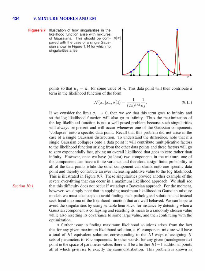
Figure 9.7 Illustration of how singularities in thelikelihood function arise with mixturesof Gaussians. This should be com-pared with the case of a single Gaus-sian shown in Figure 1.14 for which nosingularities arise.

x

p(x)

points so that µj = xn for some value of n. This data point will then contribute aterm in the likelihood function of the form

N (xn|xn, σ2j I) =

1(2π)1/2

1σj

. (9.15)

If we consider the limit σj → 0, then we see that this term goes to infinity andso the log likelihood function will also go to infinity. Thus the maximization ofthe log likelihood function is not a well posed problem because such singularitieswill always be present and will occur whenever one of the Gaussian components‘collapses’ onto a specific data point. Recall that this problem did not arise in thecase of a single Gaussian distribution. To understand the difference, note that if asingle Gaussian collapses onto a data point it will contribute multiplicative factorsto the likelihood function arising from the other data points and these factors will goto zero exponentially fast, giving an overall likelihood that goes to zero rather thaninfinity. However, once we have (at least) two components in the mixture, one ofthe components can have a finite variance and therefore assign finite probability toall of the data points while the other component can shrink onto one specific datapoint and thereby contribute an ever increasing additive value to the log likelihood.This is illustrated in Figure 9.7. These singularities provide another example of thesevere over-fitting that can occur in a maximum likelihood approach. We shall seethat this difficulty does not occur if we adopt a Bayesian approach. For the moment,Section 10.1however, we simply note that in applying maximum likelihood to Gaussian mixturemodels we must take steps to avoid finding such pathological solutions and insteadseek local maxima of the likelihood function that are well behaved. We can hope toavoid the singularities by using suitable heuristics, for instance by detecting when aGaussian component is collapsing and resetting its mean to a randomly chosen valuewhile also resetting its covariance to some large value, and then continuing with theoptimization.

A further issue in finding maximum likelihood solutions arises from the factthat for any given maximum likelihood solution, a K-component mixture will havea total of K! equivalent solutions corresponding to the K! ways of assigning Ksets of parameters to K components. In other words, for any given (nondegenerate)point in the space of parameter values there will be a further K!−1 additional pointsall of which give rise to exactly the same distribution. This problem is known as


identifiability (Casella and Berger, 2002) and is an important issue when we wish tointerpret the parameter values discovered by a model. Identifiability will also arisewhen we discuss models having continuous latent variables in Chapter 12. However,for the purposes of finding a good density model, it is irrelevant because any of theequivalent solutions is as good as any other.

Maximizing the log likelihood function (9.14) for a Gaussian mixture modelturns out to be a more complex problem than for the case of a single Gaussian. Thedifficulty arises from the presence of the summation over k that appears inside thelogarithm in (9.14), so that the logarithm function no longer acts directly on theGaussian. If we set the derivatives of the log likelihood to zero, we will no longerobtain a closed form solution, as we shall see shortly.

One approach is to apply gradient-based optimization techniques (Fletcher, 1987;Nocedal and Wright, 1999; Bishop and Nabney, 2008). Although gradient-basedtechniques are feasible, and indeed will play an important role when we discussmixture density networks in Chapter 5, we now consider an alternative approachknown as the EM algorithm which has broad applicability and which will lay thefoundations for a discussion of variational inference techniques in Chapter 10.

9.2.2 EM for Gaussian mixturesAn elegant and powerful method for finding maximum likelihood solutions for

models with latent variables is called the expectation-maximization algorithm, or EMalgorithm (Dempster et al., 1977; McLachlan and Krishnan, 1997). Later we shallgive a general treatment of EM, and we shall also show how EM can be generalizedto obtain the variational inference framework. Initially, we shall motivate the EMSection 10.1algorithm by giving a relatively informal treatment in the context of the Gaussianmixture model. We emphasize, however, that EM has broad applicability, and indeedit will be encountered in the context of a variety of different models in this book.

Let us begin by writing down the conditions that must be satisfied at a maximumof the likelihood function. Setting the derivatives of ln p(X|π, µ,Σ) in (9.14) withrespect to the means µk of the Gaussian components to zero, we obtain

0 = −N∑

n=1

πkN (xn|µk,Σk)∑j πjN (xn|µj ,Σj)︸︷︷︸

γ(znk)

Σk(xn − µk) (9.16)

where we have made use of the form (2.43) for the Gaussian distribution. Note thatthe posterior probabilities, or responsibilities, given by (9.13) appear naturally onthe right-hand side. Multiplying by Σ−1

k (which we assume to be nonsingular) andrearranging we obtain

µk =1

Nk

N∑n=1

γ(znk)xn (9.17)

where we have defined

Nk =N∑

n=1

γ(znk). (9.18)


We can interpret Nk as the effective number of points assigned to cluster k. Notecarefully the form of this solution. We see that the mean µk for the kth Gaussiancomponent is obtained by taking a weighted mean of all of the points in the data set,in which the weighting factor for data point xn is given by the posterior probabilityγ(znk) that component k was responsible for generating xn.

If we set the derivative of ln p(X|π, µ,Σ) with respect to Σk to zero, and followa similar line of reasoning, making use of the result for the maximum likelihoodsolution for the covariance matrix of a single Gaussian, we obtainSection 2.3.4

Σk =1

Nk

N∑n=1

γ(znk)(xn − µk)(xn − µk)T (9.19)

which has the same form as the corresponding result for a single Gaussian fitted tothe data set, but again with each data point weighted by the corresponding poste-rior probability and with the denominator given by the effective number of pointsassociated with the corresponding component.

Finally, we maximize ln p(X|π, µ,Σ) with respect to the mixing coefficientsπk. Here we must take account of the constraint (9.9), which requires the mixingcoefficients to sum to one. This can be achieved using a Lagrange multiplier andAppendix Emaximizing the following quantity

ln p(X|π, µ,Σ) + λ

(K∑

k=1

πk − 1

)(9.20)

which gives

0 =N∑

n=1

N (xn|µk,Σk)∑j πjN (xn|µj ,Σj)

+ λ (9.21)

where again we see the appearance of the responsibilities. If we now multiply bothsides by πk and sum over k making use of the constraint (9.9), we find λ = −N .Using this to eliminate λ and rearranging we obtain

πk =Nk

N(9.22)

so that the mixing coefficient for the kth component is given by the average respon-sibility which that component takes for explaining the data points.

It is worth emphasizing that the results (9.17), (9.19), and (9.22) do not con-stitute a closed-form solution for the parameters of the mixture model because theresponsibilities γ(znk) depend on those parameters in a complex way through (9.13).However, these results do suggest a simple iterative scheme for finding a solution tothe maximum likelihood problem, which as we shall see turns out to be an instanceof the EM algorithm for the particular case of the Gaussian mixture model. Wefirst choose some initial values for the means, covariances, and mixing coefficients.Then we alternate between the following two updates that we shall call the E step


(a)−2 0 2

−2

0

2

(b)−2 0 2

−2

0

2

(c)

L = 1

−2 0 2

−2

0

2

(d)

L = 2

−2 0 2

−2

0

2

(e)

L = 5

−2 0 2

−2

0

2

(f)

L = 20

−2 0 2

−2

0

2

Figure 9.8 Illustration of the EM algorithm using the Old Faithful set as used for the illustration of the K-meansalgorithm in Figure 9.1. See the text for details.

and the M step, for reasons that will become apparent shortly. In the expectationstep, or E step, we use the current values for the parameters to evaluate the posteriorprobabilities, or responsibilities, given by (9.13). We then use these probabilities inthe maximization step, or M step, to re-estimate the means, covariances, and mix-ing coefficients using the results (9.17), (9.19), and (9.22). Note that in so doingwe first evaluate the new means using (9.17) and then use these new values to findthe covariances using (9.19), in keeping with the corresponding result for a singleGaussian distribution. We shall show that each update to the parameters resultingfrom an E step followed by an M step is guaranteed to increase the log likelihoodfunction. In practice, the algorithm is deemed to have converged when the changeSection 9.4in the log likelihood function, or alternatively in the parameters, falls below somethreshold. We illustrate the EM algorithm for a mixture of two Gaussians applied tothe rescaled Old Faithful data set in Figure 9.8. Here a mixture of two Gaussiansis used, with centres initialized using the same values as for the K-means algorithmin Figure 9.1, and with precision matrices initialized to be proportional to the unitmatrix. Plot (a) shows the data points in green, together with the initial configura-tion of the mixture model in which the one standard-deviation contours for the two


Gaussian components are shown as blue and red circles. Plot (b) shows the resultof the initial E step, in which each data point is depicted using a proportion of blueink equal to the posterior probability of having been generated from the blue com-ponent, and a corresponding proportion of red ink given by the posterior probabilityof having been generated by the red component. Thus, points that have a significantprobability for belonging to either cluster appear purple. The situation after the firstM step is shown in plot (c), in which the mean of the blue Gaussian has moved tothe mean of the data set, weighted by the probabilities of each data point belongingto the blue cluster, in other words it has moved to the centre of mass of the blue ink.Similarly, the covariance of the blue Gaussian is set equal to the covariance of theblue ink. Analogous results hold for the red component. Plots (d), (e), and (f) showthe results after 2, 5, and 20 complete cycles of EM, respectively. In plot (f) thealgorithm is close to convergence.

Note that the EM algorithm takes many more iterations to reach (approximate)convergence compared with the K-means algorithm, and that each cycle requiressignificantly more computation. It is therefore common to run the K-means algo-rithm in order to find a suitable initialization for a Gaussian mixture model that issubsequently adapted using EM. The covariance matrices can conveniently be ini-tialized to the sample covariances of the clusters found by the K-means algorithm,and the mixing coefficients can be set to the fractions of data points assigned to therespective clusters. As with gradient-based approaches for maximizing the log like-lihood, techniques must be employed to avoid singularities of the likelihood functionin which a Gaussian component collapses onto a particular data point. It should beemphasized that there will generally be multiple local maxima of the log likelihoodfunction, and that EM is not guaranteed to find the largest of these maxima. Becausethe EM algorithm for Gaussian mixtures plays such an important role, we summarizeit below.

EM for Gaussian Mixtures

Given a Gaussian mixture model, the goal is to maximize the likelihood functionwith respect to the parameters (comprising the means and covariances of thecomponents and the mixing coefficients).

1. Initialize the means µk, covariances Σk and mixing coefficients πk, andevaluate the initial value of the log likelihood.

2. E step. Evaluate the responsibilities using the current parameter values

γ(znk) =πkN (xn|µk,Σk)

K∑j=1

πjN (xn|µj ,Σj)

. (9.23)

9.3. An Alternative View of EM 439

3. M step. Re-estimate the parameters using the current responsibilities

µnewk =

1Nk

N∑n=1

γ(znk)xn (9.24)

Σnewk =

1Nk

N∑n=1

γ(znk) (xn − µnewk ) (xn − µnew

k )T (9.25)

πnewk =

Nk

N(9.26)

where

Nk =N∑

n=1

γ(znk). (9.27)

4. Evaluate the log likelihood

ln p(X|µ,Σ, π) =N∑

n=1

ln

{K∑

k=1

πkN (xn|µk,Σk)

}(9.28)

and check for convergence of either the parameters or the log likelihood. Ifthe convergence criterion is not satisfied return to step 2.

9.3. An Alternative View of EM

In this section, we present a complementary view of the EM algorithm that recog-nizes the key role played by latent variables. We discuss this approach first of allin an abstract setting, and then for illustration we consider once again the case ofGaussian mixtures.

The goal of the EM algorithm is to find maximum likelihood solutions for mod-els having latent variables. We denote the set of all observed data by X, in which thenth row represents xT

n , and similarly we denote the set of all latent variables by Z,with a corresponding row zT

n . The set of all model parameters is denoted by θ, andso the log likelihood function is given by

ln p(X|θ) = ln

{∑Z

p(X,Z|θ)

}. (9.29)

Note that our discussion will apply equally well to continuous latent variables simplyby replacing the sum over Z with an integral.

A key observation is that the summation over the latent variables appears insidethe logarithm. Even if the joint distribution p(X,Z|θ) belongs to the exponential


family, the marginal distribution p(X|θ) typically does not as a result of this sum-mation. The presence of the sum prevents the logarithm from acting directly on thejoint distribution, resulting in complicated expressions for the maximum likelihoodsolution.

Now suppose that, for each observation in X, we were told the correspondingvalue of the latent variable Z. We shall call {X,Z} the complete data set, and weshall refer to the actual observed data X as incomplete, as illustrated in Figure 9.5.The likelihood function for the complete data set simply takes the form ln p(X,Z|θ),and we shall suppose that maximization of this complete-data log likelihood functionis straightforward.

In practice, however, we are not given the complete data set {X,Z}, but onlythe incomplete data X. Our state of knowledge of the values of the latent variablesin Z is given only by the posterior distribution p(Z|X, θ). Because we cannot usethe complete-data log likelihood, we consider instead its expected value under theposterior distribution of the latent variable, which corresponds (as we shall see) to theE step of the EM algorithm. In the subsequent M step, we maximize this expectation.If the current estimate for the parameters is denoted θold, then a pair of successiveE and M steps gives rise to a revised estimate θnew. The algorithm is initialized bychoosing some starting value for the parameters θ0. The use of the expectation mayseem somewhat arbitrary. However, we shall see the motivation for this choice whenwe give a deeper treatment of EM in Section 9.4.

In the E step, we use the current parameter values θold to find the posteriordistribution of the latent variables given by p(Z|X, θold). We then use this posteriordistribution to find the expectation of the complete-data log likelihood evaluated forsome general parameter value θ. This expectation, denoted Q(θ, θold), is given by

Q(θ, θold) =∑Z

p(Z|X, θold) ln p(X,Z|θ). (9.30)

In the M step, we determine the revised parameter estimate θnew by maximizing thisfunction

θnew = arg maxθ

Q(θ, θold). (9.31)

Note that in the definition of Q(θ, θold), the logarithm acts directly on the jointdistribution p(X,Z|θ), and so the corresponding M-step maximization will, by sup-position, be tractable.

The general EM algorithm is summarized below. It has the property, as we shallshow later, that each cycle of EM will increase the incomplete-data log likelihood(unless it is already at a local maximum).Section 9.4

The General EM Algorithm

Given a joint distribution p(X,Z|θ) over observed variables X and latent vari-ables Z, governed by parameters θ, the goal is to maximize the likelihood func-tion p(X|θ) with respect to θ.

1. Choose an initial setting for the parameters θold.


2. E step Evaluate p(Z|X, θold).

3. M step Evaluate θnew given by

θnew = arg maxθ

Q(θ, θold) (9.32)

whereQ(θ, θold) =

∑Z

p(Z|X, θold) ln p(X,Z|θ). (9.33)

4. Check for convergence of either the log likelihood or the parameter values.If the convergence criterion is not satisfied, then let

θold ← θnew (9.34)

and return to step 2.

The EM algorithm can also be used to find MAP (maximum posterior) solutionsfor models in which a prior p(θ) is defined over the parameters. In this case the EExercise 9.4step remains the same as in the maximum likelihood case, whereas in the M step thequantity to be maximized is given by Q(θ, θold) + ln p(θ). Suitable choices for theprior will remove the singularities of the kind illustrated in Figure 9.7.

Here we have considered the use of the EM algorithm to maximize a likelihoodfunction when there are discrete latent variables. However, it can also be appliedwhen the unobserved variables correspond to missing values in the data set. Thedistribution of the observed values is obtained by taking the joint distribution of allthe variables and then marginalizing over the missing ones. EM can then be usedto maximize the corresponding likelihood function. We shall show an example ofthe application of this technique in the context of principal component analysis inFigure 12.11. This will be a valid procedure if the data values are missing at random,meaning that the mechanism causing values to be missing does not depend on theunobserved values. In many situations this will not be the case, for instance if asensor fails to return a value whenever the quantity it is measuring exceeds somethreshold.

9.3.1 Gaussian mixtures revisitedWe now consider the application of this latent variable view of EM to the spe-

cific case of a Gaussian mixture model. Recall that our goal is to maximize the loglikelihood function (9.14), which is computed using the observed data set X, and wesaw that this was more difficult than for the case of a single Gaussian distributiondue to the presence of the summation over k that occurs inside the logarithm. Sup-pose then that in addition to the observed data set X, we were also given the valuesof the corresponding discrete variables Z. Recall that Figure 9.5(a) shows a ‘com-plete’ data set (i.e., one that includes labels showing which component generatedeach data point) while Figure 9.5(b) shows the corresponding ‘incomplete’ data set.The graphical model for the complete data is shown in Figure 9.9.


Figure 9.9 This shows the same graph as in Figure 9.6 except thatwe now suppose that the discrete variables zn are ob-served, as well as the data variables xn.

xn

zn

N

µ Σ

π

Now consider the problem of maximizing the likelihood for the complete dataset {X,Z}. From (9.10) and (9.11), this likelihood function takes the form

p(X,Z|µ,Σ, π) =N∏

n=1

K∏k=1

πznk

k N (xn|µk,Σk)znk (9.35)

where znk denotes the kth component of zn. Taking the logarithm, we obtain

ln p(X,Z|µ,Σ, π) =N∑

n=1

K∑k=1

znk {lnπk + lnN (xn|µk,Σk)} . (9.36)

Comparison with the log likelihood function (9.14) for the incomplete data showsthat the summation over k and the logarithm have been interchanged. The loga-rithm now acts directly on the Gaussian distribution, which itself is a member ofthe exponential family. Not surprisingly, this leads to a much simpler solution tothe maximum likelihood problem, as we now show. Consider first the maximizationwith respect to the means and covariances. Because zn is a K-dimensional vec-tor with all elements equal to 0 except for a single element having the value 1, thecomplete-data log likelihood function is simply a sum of K independent contribu-tions, one for each mixture component. Thus the maximization with respect to amean or a covariance is exactly as for a single Gaussian, except that it involves onlythe subset of data points that are ‘assigned’ to that component. For the maximizationwith respect to the mixing coefficients, we note that these are coupled for differentvalues of k by virtue of the summation constraint (9.9). Again, this can be enforcedusing a Lagrange multiplier as before, and leads to the result

πk =1N

N∑n=1

znk (9.37)

so that the mixing coefficients are equal to the fractions of data points assigned tothe corresponding components.

Thus we see that the complete-data log likelihood function can be maximizedtrivially in closed form. In practice, however, we do not have values for the latentvariables so, as discussed earlier, we consider the expectation, with respect to theposterior distribution of the latent variables, of the complete-data log likelihood.


Using (9.10) and (9.11) together with Bayes’ theorem, we see that this posteriordistribution takes the form

p(Z|X, µ,Σ, π) ∝N∏

n=1

K∏k=1

[πkN (xn|µk,Σk)]znk . (9.38)

and hence factorizes over n so that under the posterior distribution the {zn} areindependent. This is easily verified by inspection of the directed graph in Figure 9.6Exercise 9.5and making use of the d-separation criterion. The expected value of the indicatorSection 8.2variable znk under this posterior distribution is then given by

E[znk] =

∑znk

znk [πkN (xn|µk,Σk)]znk

∑znj

[πjN (xn|µj ,Σj)

]znj

=πkN (xn|µk,Σk)

K∑j=1

πjN (xn|µj ,Σj)

= γ(znk) (9.39)

which is just the responsibility of component k for data point xn. The expected valueof the complete-data log likelihood function is therefore given by

EZ[ln p(X,Z|µ,Σ, π)] =N∑

n=1

K∑k=1

γ(znk) {lnπk + lnN (xn|µk,Σk)} . (9.40)

We can now proceed as follows. First we choose some initial values for the param-eters µold, Σold and πold, and use these to evaluate the responsibilities (the E step).We then keep the responsibilities fixed and maximize (9.40) with respect to µk, Σk

and πk (the M step). This leads to closed form solutions for µnew, Σnew and πnew

given by (9.17), (9.19), and (9.22) as before. This is precisely the EM algorithm forExercise 9.8Gaussian mixtures as derived earlier. We shall gain more insight into the role of theexpected complete-data log likelihood function when we give a proof of convergenceof the EM algorithm in Section 9.4.

9.3.2 Relation to K-meansComparison of the K-means algorithm with the EM algorithm for Gaussian

mixtures shows that there is a close similarity. Whereas the K-means algorithmperforms a hard assignment of data points to clusters, in which each data point isassociated uniquely with one cluster, the EM algorithm makes a soft assignmentbased on the posterior probabilities. In fact, we can derive the K-means algorithmas a particular limit of EM for Gaussian mixtures as follows.

Consider a Gaussian mixture model in which the covariance matrices of themixture components are given by εI, where ε is a variance parameter that is shared


by all of the components, and I is the identity matrix, so that

p(x|µk,Σk) =1

(2πε)1/2exp

{− 1

2ε‖x − µk‖2

}. (9.41)

We now consider the EM algorithm for a mixture of K Gaussians of this form inwhich we treat ε as a fixed constant, instead of a parameter to be re-estimated. From(9.13) the posterior probabilities, or responsibilities, for a particular data point xn,are given by

γ(znk) =πk exp {−‖xn − µk‖2/2ε}∑j πj exp

{−‖xn − µj‖2/2ε} . (9.42)

If we consider the limit ε → 0, we see that in the denominator the term for which‖xn − µj‖2 is smallest will go to zero most slowly, and hence the responsibilitiesγ(znk) for the data point xn all go to zero except for term j, for which the responsi-bility γ(znj) will go to unity. Note that this holds independently of the values of theπk so long as none of the πk is zero. Thus, in this limit, we obtain a hard assignmentof data points to clusters, just as in the K-means algorithm, so that γ(znk) → rnk

where rnk is defined by (9.2). Each data point is thereby assigned to the clusterhaving the closest mean.

The EM re-estimation equation for the µk, given by (9.17), then reduces to theK-means result (9.4). Note that the re-estimation formula for the mixing coefficients(9.22) simply re-sets the value of πk to be equal to the fraction of data points assignedto cluster k, although these parameters no longer play an active role in the algorithm.

Finally, in the limit ε → 0 the expected complete-data log likelihood, given by(9.40), becomesExercise 9.11

EZ[ln p(X,Z|µ,Σ, π)] → −12

N∑n=1

K∑k=1

rnk‖xn − µk‖2 + const. (9.43)

Thus we see that in this limit, maximizing the expected complete-data log likelihoodis equivalent to minimizing the distortion measure J for the K-means algorithmgiven by (9.1).

Note that the K-means algorithm does not estimate the covariances of the clus-ters but only the cluster means. A hard-assignment version of the Gaussian mixturemodel with general covariance matrices, known as the elliptical K-means algorithm,has been considered by Sung and Poggio (1994).

9.3.3 Mixtures of Bernoulli distributionsSo far in this chapter, we have focussed on distributions over continuous vari-

ables described by mixtures of Gaussians. As a further example of mixture mod-elling, and to illustrate the EM algorithm in a different context, we now discuss mix-tures of discrete binary variables described by Bernoulli distributions. This modelis also known as latent class analysis (Lazarsfeld and Henry, 1968; McLachlan andPeel, 2000). As well as being of practical importance in its own right, our discus-sion of Bernoulli mixtures will also lay the foundation for a consideration of hiddenMarkov models over discrete variables.Section 13.2


Consider a set of D binary variables xi, where i = 1, . . . , D, each of which isgoverned by a Bernoulli distribution with parameter µi, so that

p(x|µ) =D∏

i=1

µxi

i (1 − µi)(1−xi) (9.44)

where x = (x1, . . . , xD)T and µ = (µ1, . . . , µD)T. We see that the individualvariables xi are independent, given µ. The mean and covariance of this distributionare easily seen to be

E[x] = µ (9.45)

cov[x] = diag{µi(1 − µi)}. (9.46)

Now let us consider a finite mixture of these distributions given by

p(x|µ, π) =K∑

k=1

πkp(x|µk) (9.47)

where µ = {µ1, . . . ,µK}, π = {π1, . . . , πK}, and

p(x|µk) =D∏

i=1

µxi

ki(1 − µki)(1−xi). (9.48)

The mean and covariance of this mixture distribution are given byExercise 9.12

E[x] =K∑

k=1

πkµk (9.49)

cov[x] =K∑

k=1

πk

{Σk + µkµT

k

}− E[x]E[x]T (9.50)

where Σk = diag {µki(1 − µki)}. Because the covariance matrix cov[x] is nolonger diagonal, the mixture distribution can capture correlations between the vari-ables, unlike a single Bernoulli distribution.

If we are given a data set X = {x1, . . . ,xN} then the log likelihood functionfor this model is given by

ln p(X|µ, π) =N∑

n=1

ln

{K∑

k=1

πkp(xn|µk)

}. (9.51)

Again we see the appearance of the summation inside the logarithm, so that themaximum likelihood solution no longer has closed form.

We now derive the EM algorithm for maximizing the likelihood function forthe mixture of Bernoulli distributions. To do this, we first introduce an explicit latent


variable z associated with each instance of x. As in the case of the Gaussian mixture,z = (z1, . . . , zK)T is a binary K-dimensional variable having a single componentequal to 1, with all other components equal to 0. We can then write the conditionaldistribution of x, given the latent variable, as

p(x|z, µ) =K∏

k=1

p(x|µk)zk (9.52)

while the prior distribution for the latent variables is the same as for the mixture ofGaussians model, so that

p(z|π) =K∏

k=1

πzk

k . (9.53)

If we form the product of p(x|z, µ) and p(z|π) and then marginalize over z, then werecover (9.47).Exercise 9.14

In order to derive the EM algorithm, we first write down the complete-data loglikelihood function, which is given by

ln p(X,Z|µ, π) =N∑

n=1

K∑k=1

znk

{ln πk

+D∑

i=1

[xni ln µki + (1 − xni) ln(1 − µki)]

}(9.54)

where X = {xn} and Z = {zn}. Next we take the expectation of the complete-datalog likelihood with respect to the posterior distribution of the latent variables to give

EZ[ln p(X,Z|µ, π)] =N∑

n=1

K∑k=1

γ(znk)

{ln πk

+D∑

i=1

[xni ln µki + (1 − xni) ln(1 − µki)]

}(9.55)

where γ(znk) = E[znk] is the posterior probability, or responsibility, of componentk given data point xn. In the E step, these responsibilities are evaluated using Bayes’theorem, which takes the form

γ(znk) = E[znk] =

∑znk

znk [πkp(xn|µk)]znk

∑znj

[πjp(xn|µj)

]znj

=πkp(xn|µk)

K∑j=1

πjp(xn|µj)

. (9.56)


If we consider the sum over n in (9.55), we see that the responsibilities enteronly through two terms, which can be written as

Nk =N∑

n=1

γ(znk) (9.57)

xk =1

Nk

N∑n=1

γ(znk)xn (9.58)

where Nk is the effective number of data points associated with component k. In theM step, we maximize the expected complete-data log likelihood with respect to theparameters µk and π. If we set the derivative of (9.55) with respect to µk equal tozero and rearrange the terms, we obtainExercise 9.15

µk = xk. (9.59)

We see that this sets the mean of component k equal to a weighted mean of thedata, with weighting coefficients given by the responsibilities that component k takesfor data points. For the maximization with respect to πk, we need to introduce aLagrange multiplier to enforce the constraint

∑k πk = 1. Following analogous

steps to those used for the mixture of Gaussians, we then obtainExercise 9.16

πk =Nk

N(9.60)

which represents the intuitively reasonable result that the mixing coefficient for com-ponent k is given by the effective fraction of points in the data set explained by thatcomponent.

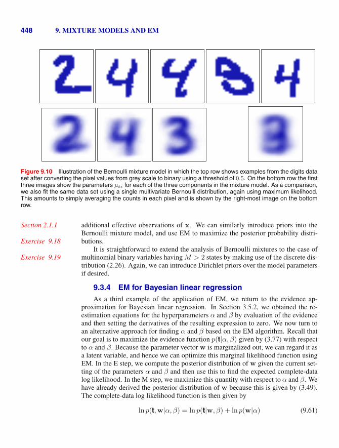
Note that in contrast to the mixture of Gaussians, there are no singularities inwhich the likelihood function goes to infinity. This can be seen by noting that thelikelihood function is bounded above because 0 � p(xn|µk) � 1. There existExercise 9.17singularities at which the likelihood function goes to zero, but these will not befound by EM provided it is not initialized to a pathological starting point, becausethe EM algorithm always increases the value of the likelihood function, until a localmaximum is found. We illustrate the Bernoulli mixture model in Figure 9.10 bySection 9.4using it to model handwritten digits. Here the digit images have been turned intobinary vectors by setting all elements whose values exceed 0.5 to 1 and setting theremaining elements to 0. We now fit a data set of N = 600 such digits, comprisingthe digits ‘2’, ‘3’, and ‘4’, with a mixture of K = 3 Bernoulli distributions byrunning 10 iterations of the EM algorithm. The mixing coefficients were initializedto πk = 1/K, and the parameters µkj were set to random values chosen uniformly inthe range (0.25, 0.75) and then normalized to satisfy the constraint that

∑j µkj = 1.

We see that a mixture of 3 Bernoulli distributions is able to find the three clusters inthe data set corresponding to the different digits.

The conjugate prior for the parameters of a Bernoulli distribution is given bythe beta distribution, and we have seen that a beta prior is equivalent to introducing


Figure 9.10 Illustration of the Bernoulli mixture model in which the top row shows examples from the digits dataset after converting the pixel values from grey scale to binary using a threshold of 0.5. On the bottom row the firstthree images show the parameters µki for each of the three components in the mixture model. As a comparison,we also fit the same data set using a single multivariate Bernoulli distribution, again using maximum likelihood.This amounts to simply averaging the counts in each pixel and is shown by the right-most image on the bottomrow.

additional effective observations of x. We can similarly introduce priors into theSection 2.1.1Bernoulli mixture model, and use EM to maximize the posterior probability distri-butions.Exercise 9.18

It is straightforward to extend the analysis of Bernoulli mixtures to the case ofmultinomial binary variables having M > 2 states by making use of the discrete dis-Exercise 9.19tribution (2.26). Again, we can introduce Dirichlet priors over the model parametersif desired.

9.3.4 EM for Bayesian linear regressionAs a third example of the application of EM, we return to the evidence ap-

proximation for Bayesian linear regression. In Section 3.5.2, we obtained the re-estimation equations for the hyperparameters α and β by evaluation of the evidenceand then setting the derivatives of the resulting expression to zero. We now turn toan alternative approach for finding α and β based on the EM algorithm. Recall thatour goal is to maximize the evidence function p(t|α, β) given by (3.77) with respectto α and β. Because the parameter vector w is marginalized out, we can regard it asa latent variable, and hence we can optimize this marginal likelihood function usingEM. In the E step, we compute the posterior distribution of w given the current set-ting of the parameters α and β and then use this to find the expected complete-datalog likelihood. In the M step, we maximize this quantity with respect to α and β. Wehave already derived the posterior distribution of w because this is given by (3.49).The complete-data log likelihood function is then given by

ln p(t,w|α, β) = ln p(t|w, β) + ln p(w|α) (9.61)


where the likelihood p(t|w, β) and the prior p(w|α) are given by (3.10) and (3.52),respectively, and y(x,w) is given by (3.3). Taking the expectation with respect tothe posterior distribution of w then gives

E [ln p(t,w|α, β)] =M

2ln( α

2π

)− α

2E[wTw

]+

N

2ln(

β

2π

)−β

2

N∑n=1

E[(tn − wTφn)2

]. (9.62)

Setting the derivatives with respect to α to zero, we obtain the M step re-estimationequationExercise 9.20

α =M

E [wTw]=

M

mTNmN + Tr(SN )

. (9.63)

An analogous result holds for β.Exercise 9.21Note that this re-estimation equation takes a slightly different form from the

corresponding result (3.92) derived by direct evaluation of the evidence function.However, they each involve computation and inversion (or eigen decomposition) ofan M ×M matrix and hence will have comparable computational cost per iteration.

These two approaches to determining α should of course converge to the sameresult (assuming they find the same local maximum of the evidence function). Thiscan be verified by first noting that the quantity γ is defined by

γ = M − α

M∑i=1

1λi + α

= M − αTr(SN ). (9.64)

At a stationary point of the evidence function, the re-estimation equation (3.92) willbe self-consistently satisfied, and hence we can substitute for γ to give

αmTNmN = γ = M − αTr(SN ) (9.65)

and solving for α we obtain (9.63), which is precisely the EM re-estimation equation.As a final example, we consider a closely related model, namely the relevance

vector machine for regression discussed in Section 7.2.1. There we used direct max-imization of the marginal likelihood to derive re-estimation equations for the hyper-parameters α and β. Here we consider an alternative approach in which we view theweight vector w as a latent variable and apply the EM algorithm. The E step involvesfinding the posterior distribution over the weights, and this is given by (7.81). In theM step we maximize the expected complete-data log likelihood, which is defined by

Ew [ln p(t|X,w, β)p(w|α)] (9.66)

where the expectation is taken with respect to the posterior distribution computedusing the ‘old’ parameter values. To compute the new parameter values we maximizewith respect to α and β to giveExercise 9.22


αnewi =

1m2

i + Σii(9.67)

(βnew)−1 =‖t − ΦmN‖2 + β−1

∑i γi

N(9.68)

These re-estimation equations are formally equivalent to those obtained by directmaxmization.Exercise 9.23

9.4. The EM Algorithm in General

The expectation maximization algorithm, or EM algorithm, is a general technique forfinding maximum likelihood solutions for probabilistic models having latent vari-ables (Dempster et al., 1977; McLachlan and Krishnan, 1997). Here we give a verygeneral treatment of the EM algorithm and in the process provide a proof that theEM algorithm derived heuristically in Sections 9.2 and 9.3 for Gaussian mixturesdoes indeed maximize the likelihood function (Csiszar and Tusnady, 1984; Hath-away, 1986; Neal and Hinton, 1999). Our discussion will also form the basis for thederivation of the variational inference framework.Section 10.1

Consider a probabilistic model in which we collectively denote all of the ob-served variables by X and all of the hidden variables by Z. The joint distributionp(X,Z|θ) is governed by a set of parameters denoted θ. Our goal is to maximizethe likelihood function that is given by

p(X|θ) =∑Z

p(X,Z|θ). (9.69)

Here we are assuming Z is discrete, although the discussion is identical if Z com-prises continuous variables or a combination of discrete and continuous variables,with summation replaced by integration as appropriate.

We shall suppose that direct optimization of p(X|θ) is difficult, but that opti-mization of the complete-data likelihood function p(X,Z|θ) is significantly easier.Next we introduce a distribution q(Z) defined over the latent variables, and we ob-serve that, for any choice of q(Z), the following decomposition holds

ln p(X|θ) = L(q, θ) + KL(q‖p) (9.70)

where we have defined

L(q, θ) =∑Z

q(Z) ln{

p(X,Z|θ)q(Z)

}(9.71)

KL(q‖p) = −∑Z

q(Z) ln{

p(Z|X, θ)q(Z)

}. (9.72)

Note that L(q, θ) is a functional (see Appendix D for a discussion of functionals)of the distribution q(Z), and a function of the parameters θ. It is worth studying

9.4. The EM Algorithm in General 451

Figure 9.11 Illustration of the decomposition givenby (9.70), which holds for any choiceof distribution q(Z). Because theKullback-Leibler divergence satisfiesKL(q‖p) � 0, we see that the quan-tity L(q, θ) is a lower bound on the loglikelihood function ln p(X|θ).

ln p(X|θ)L(q, θ)

KL(q||p)

carefully the forms of the expressions (9.71) and (9.72), and in particular noting thatthey differ in sign and also that L(q, θ) contains the joint distribution of X and Zwhile KL(q‖p) contains the conditional distribution of Z given X. To verify thedecomposition (9.70), we first make use of the product rule of probability to giveExercise 9.24

ln p(X,Z|θ) = ln p(Z|X, θ) + ln p(X|θ) (9.73)

which we then substitute into the expression for L(q, θ). This gives rise to two terms,one of which cancels KL(q‖p) while the other gives the required log likelihoodln p(X|θ) after noting that q(Z) is a normalized distribution that sums to 1.

From (9.72), we see that KL(q‖p) is the Kullback-Leibler divergence betweenq(Z) and the posterior distribution p(Z|X, θ). Recall that the Kullback-Leibler di-vergence satisfies KL(q‖p) � 0, with equality if, and only if, q(Z) = p(Z|X, θ). ItSection 1.6.1therefore follows from (9.70) that L(q, θ) � ln p(X|θ), in other words that L(q, θ)is a lower bound on ln p(X|θ). The decomposition (9.70) is illustrated in Fig-ure 9.11.

The EM algorithm is a two-stage iterative optimization technique for findingmaximum likelihood solutions. We can use the decomposition (9.70) to define theEM algorithm and to demonstrate that it does indeed maximize the log likelihood.Suppose that the current value of the parameter vector is θold. In the E step, thelower bound L(q, θold) is maximized with respect to q(Z) while holding θold fixed.The solution to this maximization problem is easily seen by noting that the valueof ln p(X|θold) does not depend on q(Z) and so the largest value of L(q, θold) willoccur when the Kullback-Leibler divergence vanishes, in other words when q(Z) isequal to the posterior distribution p(Z|X, θold). In this case, the lower bound willequal the log likelihood, as illustrated in Figure 9.12.

In the subsequent M step, the distribution q(Z) is held fixed and the lower boundL(q, θ) is maximized with respect to θ to give some new value θnew. This willcause the lower bound L to increase (unless it is already at a maximum), which willnecessarily cause the corresponding log likelihood function to increase. Because thedistribution q is determined using the old parameter values rather than the new valuesand is held fixed during the M step, it will not equal the new posterior distributionp(Z|X, θnew), and hence there will be a nonzero KL divergence. The increase in thelog likelihood function is therefore greater than the increase in the lower bound, as


Figure 9.12 Illustration of the E step ofthe EM algorithm. The qdistribution is set equal tothe posterior distribution forthe current parameter val-ues θold, causing the lowerbound to move up to thesame value as the log like-lihood function, with the KLdivergence vanishing. ln p(X|θold)L(q, θold)

KL(q||p) = 0

shown in Figure 9.13. If we substitute q(Z) = p(Z|X, θold) into (9.71), we see that,after the E step, the lower bound takes the form

L(q, θ) =∑Z

p(Z|X, θold) ln p(X,Z|θ) −∑Z

p(Z|X, θold) ln p(Z|X, θold)

= Q(θ, θold) + const (9.74)

where the constant is simply the negative entropy of the q distribution and is there-fore independent of θ. Thus in the M step, the quantity that is being maximized is theexpectation of the complete-data log likelihood, as we saw earlier in the case of mix-tures of Gaussians. Note that the variable θ over which we are optimizing appearsonly inside the logarithm. If the joint distribution p(Z,X|θ) comprises a member ofthe exponential family, or a product of such members, then we see that the logarithmwill cancel the exponential and lead to an M step that will be typically much simplerthan the maximization of the corresponding incomplete-data log likelihood functionp(X|θ).

The operation of the EM algorithm can also be viewed in the space of parame-ters, as illustrated schematically in Figure 9.14. Here the red curve depicts the (in-

Figure 9.13 Illustration of the M step of the EMalgorithm. The distribution q(Z)is held fixed and the lower boundL(q, θ) is maximized with respectto the parameter vector θ to givea revised value θnew. Because theKL divergence is nonnegative, thiscauses the log likelihood ln p(X|θ)to increase by at least as much asthe lower bound does.

ln p(X|θnew)L(q, θnew)

KL(q||p)

9.4. The EM Algorithm in General 453

Figure 9.14 The EM algorithm involves alter-nately computing a lower boundon the log likelihood for the cur-rent parameter values and thenmaximizing this bound to obtainthe new parameter values. Seethe text for a full discussion.

θold θnew

L (q, θ)

ln p(X|θ)

complete data) log likelihood function whose value we wish to maximize. We startwith some initial parameter value θold, and in the first E step we evaluate the poste-rior distribution over latent variables, which gives rise to a lower bound L(θ, θ(old))whose value equals the log likelihood at θ(old), as shown by the blue curve. Note thatthe bound makes a tangential contact with the log likelihood at θ(old), so that bothcurves have the same gradient. This bound is a convex function having a uniqueExercise 9.25maximum (for mixture components from the exponential family). In the M step, thebound is maximized giving the value θ(new), which gives a larger value of log likeli-hood than θ(old). The subsequent E step then constructs a bound that is tangential atθ(new) as shown by the green curve.

For the particular case of an independent, identically distributed data set, Xwill comprise N data points {xn} while Z will comprise N corresponding latentvariables {zn}, where n = 1, . . . , N . From the independence assumption, we havep(X,Z) =

∏n p(xn, zn) and, by marginalizing over the {zn} we have p(X) =∏

n p(xn). Using the sum and product rules, we see that the posterior probabilitythat is evaluated in the E step takes the form

p(Z|X, θ) =p(X,Z|θ)∑

Z

p(X,Z|θ)=

N∏n=1

p(xn, zn|θ)

∑Z

N∏n=1

p(xn, zn|θ)

=N∏

n=1

p(zn|xn, θ) (9.75)

and so the posterior distribution also factorizes with respect to n. In the case ofthe Gaussian mixture model this simply says that the responsibility that each of themixture components takes for a particular data point xn depends only on the valueof xn and on the parameters θ of the mixture components, not on the values of theother data points.

We have seen that both the E and the M steps of the EM algorithm are increas-ing the value of a well-defined bound on the log likelihood function and that the


complete EM cycle will change the model parameters in such a way as to causethe log likelihood to increase (unless it is already at a maximum, in which case theparameters remain unchanged).

We can also use the EM algorithm to maximize the posterior distribution p(θ|X)for models in which we have introduced a prior p(θ) over the parameters. To see this,we note that as a function of θ, we have p(θ|X) = p(θ,X)/p(X) and so

ln p(θ|X) = ln p(θ,X) − ln p(X). (9.76)

Making use of the decomposition (9.70), we have

ln p(θ|X) = L(q, θ) + KL(q‖p) + ln p(θ) − ln p(X)� L(q, θ) + ln p(θ) − ln p(X). (9.77)

where ln p(X) is a constant. We can again optimize the right-hand side alternatelywith respect to q and θ. The optimization with respect to q gives rise to the same E-step equations as for the standard EM algorithm, because q only appears in L(q, θ).The M-step equations are modified through the introduction of the prior term ln p(θ),which typically requires only a small modification to the standard maximum likeli-hood M-step equations.

The EM algorithm breaks down the potentially difficult problem of maximizingthe likelihood function into two stages, the E step and the M step, each of which willoften prove simpler to implement. Nevertheless, for complex models it may be thecase that either the E step or the M step, or indeed both, remain intractable. Thisleads to two possible extensions of the EM algorithm, as follows.

The generalized EM, or GEM, algorithm addresses the problem of an intractableM step. Instead of aiming to maximize L(q, θ) with respect to θ, it seeks insteadto change the parameters in such a way as to increase its value. Again, becauseL(q, θ) is a lower bound on the log likelihood function, each complete EM cycle ofthe GEM algorithm is guaranteed to increase the value of the log likelihood (unlessthe parameters already correspond to a local maximum). One way to exploit theGEM approach would be to use one of the nonlinear optimization strategies, suchas the conjugate gradients algorithm, during the M step. Another form of GEMalgorithm, known as the expectation conditional maximization, or ECM, algorithm,involves making several constrained optimizations within each M step (Meng andRubin, 1993). For instance, the parameters might be partitioned into groups, and theM step is broken down into multiple steps each of which involves optimizing one ofthe subset with the remainder held fixed.

We can similarly generalize the E step of the EM algorithm by performing apartial, rather than complete, optimization of L(q, θ) with respect to q(Z) (Neal andHinton, 1999). As we have seen, for any given value of θ there is a unique maximumof L(q, θ) with respect to q(Z) that corresponds to the posterior distribution qθ(Z) =p(Z|X, θ) and that for this choice of q(Z) the bound L(q, θ) is equal to the loglikelihood function ln p(X|θ). It follows that any algorithm that converges to theglobal maximum of L(q, θ) will find a value of θ that is also a global maximumof the log likelihood ln p(X|θ). Provided p(X,Z|θ) is a continuous function of θ

Exercises 455

then, by continuity, any local maximum of L(q, θ) will also be a local maximum ofln p(X|θ).

Consider the case of N independent data points x1, . . . ,xN with correspondinglatent variables z1, . . . , zN . The joint distribution p(X,Z|θ) factorizes over the datapoints, and this structure can be exploited in an incremental form of EM in whichat each EM cycle only one data point is processed at a time. In the E step, insteadof recomputing the responsibilities for all of the data points, we just re-evaluate theresponsibilities for one data point. It might appear that the subsequent M step wouldrequire computation involving the responsibilities for all of the data points. How-ever, if the mixture components are members of the exponential family, then theresponsibilities enter only through simple sufficient statistics, and these can be up-dated efficiently. Consider, for instance, the case of a Gaussian mixture, and supposewe perform an update for data point m in which the corresponding old and newvalues of the responsibilities are denoted γold(zmk) and γnew(zmk). In the M step,the required sufficient statistics can be updated incrementally. For instance, for themeans the sufficient statistics are defined by (9.17) and (9.18) from which we obtainExercise 9.26

µnewk = µold

k +(

γnew(zmk) − γold(zmk)Nnew

k

)(xm − µold

k

)(9.78)

together withNnew

k = Noldk + γnew(zmk) − γold(zmk). (9.79)

The corresponding results for the covariances and the mixing coefficients are analo-gous.

Thus both the E step and the M step take fixed time that is independent of thetotal number of data points. Because the parameters are revised after each data point,rather than waiting until after the whole data set is processed, this incremental ver-sion can converge faster than the batch version. Each E or M step in this incrementalalgorithm is increasing the value of L(q, θ) and, as we have shown above, if thealgorithm converges to a local (or global) maximum of L(q, θ), this will correspondto a local (or global) maximum of the log likelihood function ln p(X|θ).

Exercises9.1 (�) www Consider the K-means algorithm discussed in Section 9.1. Show that as

a consequence of there being a finite number of possible assignments for the set ofdiscrete indicator variables rnk, and that for each such assignment there is a uniqueoptimum for the {µk}, the K-means algorithm must converge after a finite numberof iterations.

9.2 (�) Apply the Robbins-Monro sequential estimation procedure described in Sec-tion 2.3.5 to the problem of finding the roots of the regression function given bythe derivatives of J in (9.1) with respect to µk. Show that this leads to a stochasticK-means algorithm in which, for each data point xn, the nearest prototype µk isupdated using (9.5).


9.3 (�) www Consider a Gaussian mixture model in which the marginal distributionp(z) for the latent variable is given by (9.10), and the conditional distribution p(x|z)for the observed variable is given by (9.11). Show that the marginal distributionp(x), obtained by summing p(z)p(x|z) over all possible values of z, is a Gaussianmixture of the form (9.7).

9.4 (�) Suppose we wish to use the EM algorithm to maximize the posterior distri-bution over parameters p(θ|X) for a model containing latent variables, where X isthe observed data set. Show that the E step remains the same as in the maximumlikelihood case, whereas in the M step the quantity to be maximized is given byQ(θ, θold) + ln p(θ) where Q(θ, θold) is defined by (9.30).

9.5 (�) Consider the directed graph for a Gaussian mixture model shown in Figure 9.6.By making use of the d-separation criterion discussed in Section 8.2, show that theposterior distribution of the latent variables factorizes with respect to the differentdata points so that

p(Z|X, µ,Σ, π) =N∏

n=1

p(zn|xn, µ,Σ, π). (9.80)

9.6 (� �) Consider a special case of a Gaussian mixture model in which the covari-ance matrices Σk of the components are all constrained to have a common valueΣ. Derive the EM equations for maximizing the likelihood function under such amodel.

9.7 (�) www Verify that maximization of the complete-data log likelihood (9.36) fora Gaussian mixture model leads to the result that the means and covariances of eachcomponent are fitted independently to the corresponding group of data points, andthe mixing coefficients are given by the fractions of points in each group.

9.8 (�) www Show that if we maximize (9.40) with respect to µk while keeping theresponsibilities γ(znk) fixed, we obtain the closed form solution given by (9.17).

9.9 (�) Show that if we maximize (9.40) with respect to Σk and πk while keeping theresponsibilities γ(znk) fixed, we obtain the closed form solutions given by (9.19)and (9.22).

9.10 (� �) Consider a density model given by a mixture distribution

p(x) =K∑

k=1

πkp(x|k) (9.81)

and suppose that we partition the vector x into two parts so that x = (xa,xb).Show that the conditional density p(xb|xa) is itself a mixture distribution and findexpressions for the mixing coefficients and for the component densities.

Exercises 457

9.11 (�) In Section 9.3.2, we obtained a relationship between K means and EM forGaussian mixtures by considering a mixture model in which all components havecovariance εI. Show that in the limit ε → 0, maximizing the expected complete-data log likelihood for this model, given by (9.40), is equivalent to minimizing thedistortion measure J for the K-means algorithm given by (9.1).

9.12 (�) www Consider a mixture distribution of the form

p(x) =K∑

k=1

πkp(x|k) (9.82)

where the elements of x could be discrete or continuous or a combination of these.Denote the mean and covariance of p(x|k) by µk and Σk, respectively. Show thatthe mean and covariance of the mixture distribution are given by (9.49) and (9.50).

9.13 (� �) Using the re-estimation equations for the EM algorithm, show that a mix-ture of Bernoulli distributions, with its parameters set to values corresponding to amaximum of the likelihood function, has the property that

E[x] =1N

N∑n=1

xn ≡ x. (9.83)

Hence show that if the parameters of this model are initialized such that all compo-nents have the same mean µk = µ for k = 1, . . . , K, then the EM algorithm willconverge after one iteration, for any choice of the initial mixing coefficients, and thatthis solution has the property µk = x. Note that this represents a degenerate case ofthe mixture model in which all of the components are identical, and in practice wetry to avoid such solutions by using an appropriate initialization.

9.14 (�) Consider the joint distribution of latent and observed variables for the Bernoullidistribution obtained by forming the product of p(x|z, µ) given by (9.52) and p(z|π)given by (9.53). Show that if we marginalize this joint distribution with respect to z,then we obtain (9.47).

9.15 (�) www Show that if we maximize the expected complete-data log likelihoodfunction (9.55) for a mixture of Bernoulli distributions with respect to µk, we obtainthe M step equation (9.59).

9.16 (�) Show that if we maximize the expected complete-data log likelihood function(9.55) for a mixture of Bernoulli distributions with respect to the mixing coefficientsπk, using a Lagrange multiplier to enforce the summation constraint, we obtain theM step equation (9.60).

9.17 (�) www Show that as a consequence of the constraint 0 � p(xn|µk) � 1 forthe discrete variable xn, the incomplete-data log likelihood function for a mixtureof Bernoulli distributions is bounded above, and hence that there are no singularitiesfor which the likelihood goes to infinity.


9.18 (� �) Consider a Bernoulli mixture model as discussed in Section 9.3.3, togetherwith a prior distribution p(µk|ak, bk) over each of the parameter vectors µk givenby the beta distribution (2.13), and a Dirichlet prior p(π|α) given by (2.38). Derivethe EM algorithm for maximizing the posterior probability p(µ, π|X).

9.19 (� �) Consider a D-dimensional variable x each of whose components i is itself amultinomial variable of degree M so that x is a binary vector with components xij

where i = 1, . . . , D and j = 1, . . . , M , subject to the constraint that∑

j xij = 1 forall i. Suppose that the distribution of these variables is described by a mixture of thediscrete multinomial distributions considered in Section 2.2 so that

p(x) =K∑

k=1

πkp(x|µk) (9.84)

where

p(x|µk) =D∏

i=1

M∏j=1

µxij

kij . (9.85)

The parameters µkij represent the probabilities p(xij = 1|µk) and must satisfy0 � µkij � 1 together with the constraint

∑j µkij = 1 for all values of k and i.

Given an observed data set {xn}, where n = 1, . . . , N , derive the E and M stepequations of the EM algorithm for optimizing the mixing coefficients πk and thecomponent parameters µkij of this distribution by maximum likelihood.

9.20 (�) www Show that maximization of the expected complete-data log likelihoodfunction (9.62) for the Bayesian linear regression model leads to the M step re-estimation result (9.63) for α.

9.21 (� �) Using the evidence framework of Section 3.5, derive the M-step re-estimationequations for the parameter β in the Bayesian linear regression model, analogous tothe result (9.63) for α.

9.22 (� �) By maximization of the expected complete-data log likelihood defined by(9.66), derive the M step equations (9.67) and (9.68) for re-estimating the hyperpa-rameters of the relevance vector machine for regression.

9.23 (� �) www In Section 7.2.1 we used direct maximization of the marginal like-lihood to derive the re-estimation equations (7.87) and (7.88) for finding values ofthe hyperparameters α and β for the regression RVM. Similarly, in Section 9.3.4we used the EM algorithm to maximize the same marginal likelihood, giving there-estimation equations (9.67) and (9.68). Show that these two sets of re-estimationequations are formally equivalent.

9.24 (�) Verify the relation (9.70) in which L(q, θ) and KL(q‖p) are defined by (9.71)and (9.72), respectively.

Exercises 459

9.25 (�) www Show that the lower bound L(q, θ) given by (9.71), with q(Z) =p(Z|X, θ(old)), has the same gradient with respect to θ as the log likelihood functionln p(X|θ) at the point θ = θ(old).

9.26 (�) www Consider the incremental form of the EM algorithm for a mixture ofGaussians, in which the responsibilities are recomputed only for a specific data pointxm. Starting from the M-step formulae (9.17) and (9.18), derive the results (9.78)and (9.79) for updating the component means.

9.27 (� �) Derive M-step formulae for updating the covariance matrices and mixingcoefficients in a Gaussian mixture model when the responsibilities are updated in-crementally, analogous to the result (9.78) for updating the means.

Documents

Mixture Models and EM - Penn State College of …rtc12/CSE586Spring2010/papers/prmlMixturesEM.pdf · Mixture Models and EM ... Gaussian mixture models are widely used in data mining,