Mixing Enhancement in 3D MHD Channel Flowby Boundary Electrical Potential Actuation

Lixiang Luo and Eugenio Schuster

Abstract— An electrically conductive fluid flowing inside achannel is prone to be affected by enormous magnetohydrody-namics (MHD) effects when the fluid interacts with an imposedmagnetic field. Such effects often leads to higher pressure dropand lower heat transfer rate due to laminarization. Activeboundary control, in either open loop or closed loop, can beused to enhance mixing and potentially increase heat transferrate. Open-loop controllers are in general more sensitive touncertainties of the system, which may result in a poorerperformance. A closed-loop controller is proposed based on thelinearized simplified magnetohydronamic (LSMHD) model. Mi-cro pressure sensors and electrodes are embedded into the wallsfor measurement and actuation. Using the boundary vorticityflux as the input, the proposed feedback controller regulatesthe boundary electric potential at the channel walls in orderto increase turbulence and mixing. By reversing the sign of afeedback controller designed to stabilize the LSMHD systems, adestabilizing controllers is achieved and used to excite multipleFourier modes in simulations. The simulation results providedby a 3D simplified magnetohydronamic (SMHD) simulator showthat the reversed controller successfully increases the turbulenceinside an otherwise strongly stable MHD flow.

I. INTRODUCTION

Magnetohydrodynamic (MHD) problems arise in manyapplications. One of them is cooling systems, where a liquidmetal is often used as a heat transfer media. Because oftheir high thermal conductivity and high boiling point, liquidmetals are highly favorable for applications with extremeconditions such as a fusion reactor cooling blanket. In thisapplication certain liquid metals may also serve as fuelbreeders as they react with the neutrons generated by thefusion reactions. In a fusion reactor a strong magnetic fieldis used to confine the plasma where the fusion reactiontakes place; and this magnetic field inevitably affects theelectrically conductive fluid in the cooling blanket. Whenthe electrically conductive fluid flows in the presence of atransverse magnetic field, it generates an electric field dueto charge separation and a subsequent electric current. Theinteraction between the induced current and the imposedmagnetic field generates a body force, called the Lorentzforce, which acts on the fluid itself. As the force acts inthe opposite direction of the flow, it is necessary to increasethe flow pressure gradient in order to maintain the averagevelocity of the flow and more power is needed to pump theliquid through the channel. In addition, the MHD effectstend to suppress perturbations and to laminarize the flow,

This work was supported by the NSF CAREER award program (ECCS–0645086).

Lixiang Luo and Eugenio Schuster are with the Department of Mechan-ical Engineering and Mechanics, Lehigh University, Bethlehem, PA 18015,USA (lixiang.luo@lehigh.edu, schuster@lehigh.edu)

reducing heat transfer rate as a consequence. A good reviewof the current status in this area can be found in [1].

Active control of fluid systems, implemented through mi-cro electro-mechanical (MEM) or electro-magnetic actuatorsand sensors, can be used to achieve optimally the desiredlevel of stability (when suppression of turbulence is desired)or instability (when enhancement of mixing is desired).The benefits of managing and controlling unsteady flowsin engineering applications can be significant. This areahas attracted much interest and has dramatically advancedin recent years [2], [3], [4], [5]. The boundary control ofMHD flows has been considered for decades [6], [7], [8],[9], [10]. Research subjects range from strongly coupledMHD problems, like liquid metal and melted salt flows, toweakly coupled MHD problems, like salt water flows. Earlyresearch mostly focused on passive and open loop control.This situation is partly due to the complexity of the coupledMHD equations.

Our prior work includes several feedback control schemesfor mixing enhancement in 2D MHD channel flows based onmechanical actuation at the boundary via blowing and suc-tion. Micro-jets, pressure sensors, and magnetic field sensorsembedded into the walls of the flow domain were consideredin [11] to find a feedback control law that is optimal withrespect to a cost functional related to a mixing measure. Theeffectiveness of the proposed controller for mixing and heattransfer enhancement has been illustrated in [12]. Anotherclosed-loop controller was proposed in [13] based on a fixed-structure control law optimally tuned by extremum seeking.The moving speed of the fixed-structure traveling-wave-likeboundary control was optimized in order to maximize a costfunction defined as the heat transfer rate at the channel outlet.The numerical simulations confirmed that both closed-loopcontrol schemes are effective in enhancing mixing and heattransfer by introducing 2D turbulence.

In this work we move to the problem of mixing enhance-ment in 3D MHD channel flows where only electromagneticactuation is employed. We follow a linearization approach todevelop a feedback controller based on the simplified MHD(SMHD) model. Spectral transformations are employed totransform the PDE system into a series of one-dimensionalODE systems. A feedback control law is designed to stabilizeone of the ODE systems. The sign of the resulting controlleris then reversed, which results into a linearly unstable feed-back loop. By imposing a saturation limit for the controller,we successfully bound the instability and maintain a highlevel of turbulence near the walls. Simulation results areprovided to illustrate the effectiveness of the controller.

Fig. 1. System geometry

This article is organized as follows. In Section II, we statethe system equations for incompressible SMHD flows, andderive the linearized version required for control synthesis.In Section III, the controller for the LSMHD system isdesigned, and the sign reversing procedure is discussed.In Section IV, simulation results are given in a typicalmagnetohydrodynamic physical setting. Section V closes thepaper stating the conclusion and the identified future work.

II. PROBLEM STATEMENT

We consider a 3D, incompressible, electrically conductingfluid flowing between two parallel plates (0<x<d = 2π ,0<z<π and 0<y<1) along the x-direction, as illustratedin Fig. 1, where an external magnetic field B0 is imposedperpendicularly to the plates, i.e., in the wall-normal ydirection. This flow was first investigated experimentallyand theoretically by Hartmann [14]. The mass flux Q isfixed. A uniform pressure gradient Px in the x-direction isrequired to balance the boundary drag force and the bodyforce due to the MHD effects. Space variables x, y, z, timet, velocity v and magnetic induction B are converted to theirdimensionless forms:

x =x∗

L, y =

y∗

L, z =

z∗

L,

B =B∗

B0, v =

v∗

U0, j =

j∗

U0B0, t =

t∗U0

L,

where L, U0 and B0 are dimensional reference length, veloc-ity and magnetic field. Variables denoted by the star notationare dimensional quantities.

The vector variables are defined as

v(x,y, t) = u(x,y, t)x+ v(x,y, t)y+w(x,y, t)z,B(x,y, t) = Bu(x,y, t)x+Bv(x,y, t)y+Bw(x,y, t)z,

where x, y and z are unit vectors in the x, y and z directions,respectively. The dimensionless governing equations for theMHD channel flow are given by

∂v∂ t

=1

Re∇2v−∇P− (v ·∇)v−N(j×B) ,

∂B∂ t

=1

Rem∇2B+∇× (v×B),

j = 1Rem

∇×B,

∇ ·v = 0, ∇ ·B = 0.

The characteristic numbers, including Reynolds number,magnetic Reynolds number, Stuart number and Hartmannnumber are defined as:

Re =U0L

ν, Rem = µσU0L, N =

σB20L

ρU0, Ha =

√NRe.

The Hartmann number is used to indicate the interactionlevel between the magnetic field and the velocity field. Thephysical properties of the fluid, including the mass densityρ , the dynamic viscosity ν , the electrical conductivity σ andthe magnetic permeability µ , are all assumed constant.

In this paper, we consider MHD flows at low magneticReynolds numbers (Rem�1), which are also called sim-plified MHD (SMHD) flows. In these flows the inducedmagnetic field is negligible in comparison with the imposedmagnetic field. The 3D SMHD channel flow is describedby slightly modified incompressible Navier-Stokes (N-S)equations and a Poisson’s equation for the electric potential:

∂v∂ t

+(v·∇)v=−∇p+1

Re∇2v+N [(−∇ϕ+v×B0)×B0] , (1)

∇2ϕ = ∇ · (v×B0) = B0 ·ω, (2)∇ ·v = 0, (3)

where ω = ∇ × v is the vorticity, B0 = y is the imposedmagnetic field (which is simply a unit vector due to the non-dimensionalization). A detailed derivation can be found in[15]. The boundary conditions are given by

v(x,±1, t) = 0, ϕ (x,−1, t) = ϕb, ϕ (x,1, t) = ϕp,

where ϕb and ϕp are determined by the controller.The N-S equation for channel flows can be written in terms

of the wall-normal velocity v and the wall-normal componentof the vorticity η . The other components of the velocity canbe recovered by (3) and the definition of the wall-normalvorticity (η = ∂zu− ∂xw). Following a procedure similar tothe derivation of the Orr-Sommerfeld and Squire equations,we can write the linearized SMHD equations as follows:

��∂∂ t

+U∂∂x

�∆−U �� ∂

∂x− 1

Re∆2 +N

∂ 2

∂y2

�v = 0,

�∂∂ t

+U∂∂x

− 1Re

∆+N�

η =−U � ∂v∂ z

+N�

∂ 2ϕ∂x2 +

∂ 2ϕ∂ z2

�,

∆ϕ = η .

where ∆ = ∇2 =�D2 − k2

0�

is the Laplacian operator and Dis the first derivative operator in the y direction.

By computing the Fourier transforms in the x and zdirections, the system above can be divided into a series ofindependent ODE systems, each representing the evolutionof a particular wave number pair {kx,kz} (see, for example,[16], for more details):

∆v =�

1Re

∆2 − ikxU∆+ ikxU ��+ND2�

v, (4)

η =�−ikzU ��v+

�1

Re∆− ikxU −N

�η +

�Nk2

0�

ϕ. (5)

Note that both v and η have been transformed into Fourierspace (whether the variables are either in physical spaceor Fourier space can be determined by the context). Inorder to write the system in a standard state-space form, theoperator D2 is discretized by the Chebyshev collocation. TheLaplacian operator can be inverted if appropriate boundaryconditions are given when constructing the D2 operatormatrix. This is done by using the Differentiation MatrixSuite developed by Weideman & Reddy [17]. The Poisson’sequation for the electric potential can also be inverted in asimilar manner.

The output of the system is selected as the boundaryvorticity flux, defined as.

σ = (σb,σp)T =

�∂η∂y

����y=−1

,∂η∂y

����y=1

�T

.

The physical viability and numerical convenience leads tothis selection. From a physical perspective, we know thatalthough the boundary vorticity flux can not be measureddirectly it can be determined by boundary pressure gradients,which can be measured [18]. From a numerical perspective,it is straightforward to calculate the vorticity flux by takingthe first derivative of the vorticity at the boundaries. Then,the equations can be further written as

v = Mvvv, (6)η = Mvη v+Mηη η +Mϕη ϕ, (7)ϕ = Mηϕ η +Mθϕ θ , (8)σ = Mησ η , (9)

where θ = (ϕb,ϕp)T is the system input and

Mvv = ∆−1�

1Re

∆2 − ikxU∆+ ikxU ��+ND2�,

Mvη =−ikzU �,

Mηη =1

Re∆− ikxU −N,

Mϕη = Nk20.

Mηϕ and Mθϕ are both results of the inversion of the ∆operator. Mησ is a part of the D operator that computes thefirst derivatives at the boundaries.

A standard state-space model G0 can be finally written as

ξ = Aξ +Bθ ,σ =Cξ ,

where ξ = (v,η)T and

A =

�Mvv 0Mvη Mηη +Mϕη Mηϕ

�, B =

�0

Mϕη Mθϕ

�,

C =�

0 Mησ�.

This LSMHD system model serves as the basis for thecontroller design.

III. CONTROLLER DESIGN

The LSMHD system is constructed by performing a dis-cretization in the y coordinate on a grid of 64 Chebyshevcollocation points in order to form a set of linear ODE’s. Theresulting system is then analyzed by modern control tech-niques. The system dynamics consists of two major parts:velocity v and vorticity η . The velocity equation (6) closelyresembles the Orr-Sommerfeld equation, while the vorticityequation (7) resembles the Squire equation. They differ onlyby two extra terms produced by the Lorentz force. Like theOrr-Sommerfeld/Squire system, the velocity equation has itsindependent dynamics and the vorticity equation is drivenby the velocity. The original Orr-Sommerfeld equation hasa critical Reynolds number (Re≈5772), where the equationturns linearly unstable [16], [19]. The extra Lorentz forceterms tends however to stabilize the system, as indicated bythe movement of eigenvalues towards the left-half complexplane when magnetic fields are imposed (Table I).

TABLE ISIX MOST SIGNIFICANT EIGENVALUES (Re = 6500, kx =1, kz =0)

Ha=0 Ha=0.8 Ha=2.5

0.0011±0.256i−0.0089±0.991i−0.0265±0.973i−0.0436±0.956i−0.0436±0.956i−0.0440±0.956i

−0.0026±0.255i−0.0087±0.981i−0.0258±0.964i−0.0423±0.947i−0.0423±0.947i−0.0428±0.947i

−0.0075±0.912i−0.0209±0.899i−0.0289±0.249i−0.0333±0.886i−0.0338±0.887i−0.0344±0.886i

The objective of our controller is indeed to destabilizethe system so that it becomes linearly unstable when animposed magnetic field is present. First, we perform an H∞

normalized coprime factor controller synthesis to generatea stabilizing controller. The H∞ synthesis is done upon analready stable system (Re = 6500, kx=1, kz=0, Ha=2.5).The result of the H∞ synthesis has the same order as theoriginal system G0. To simplify the implementation of thecontroller in the numerical simulator, model reduction iscarried out to represent the controller as a second-ordersystem. Next, the sign of the resulting controller is reversedin order to destabilize the closed-loop system with positivefeedback. The reversed controller K takes a standard state-space form

x = AKx+BKσ ,

θ =CKx+DKσ .

Finally, a saturation limit is imposed on the actuator to ensurethe system remains bounded.

TABLE IIMOST SIGNIFICANT EIGENVALUES (Re = 6500, kx =1, kz =0)

Ha=0.8 Ha=2.5

Open loop −0.0026±0.255i −0.0075±0.912i

Closed loop 0.0149±0.116i 0.2953±0.083i

��

�

�

���������

� ��

� ����� �

��������

Fig. 2. Feedback loop overview

A simple closed-loop architecture based on this controller,as illustrated in Fig. 2, can be linearly unstable. This canbe seen from Table II where both stable systems in Table Ibecome linearly unstable under the effect of the controller K.Although the controller is designed to excite the kx=1, kz=0mode, it is also effective in exciting higher order modes,which is necessary to achieve the desired turbulence level.Therefore, in the simulation results presented in the followingsection all the Fourier modes are excited using the samecontroller K and the same saturation limit.

IV. SIMULATION RESULTS

The numerical simulations are carried out by a modifiedNavier-Stokes solver, originally written by T. Bewley [20].The equations are discretized using FFT in the x and zdirections and finite differences in the y direction, whichis also called the pseudospectral method. Time integra-tion is done using a fractional step method along with ahybrid Runge-Kutta/Crank-Nicolson scheme. Linear termsare treated implicitly by the Crank-Nicolson method andnonlinear terms are treated explicitly by the Runge-Kuttamethod. The divergence-free condition is fulfilled by thefractional step method. The controller is implemented asa second order time-evolving system using fully implicittime integration. All the simulations are carried out for thesame flow domain: 0<x<d = 2π , 0<z<π and 0<y<1.The same mesh is used in all the simulations presented inthis section (same number of grid points in all directions:NX=NY=NY=64).

A. MHD flows with no control

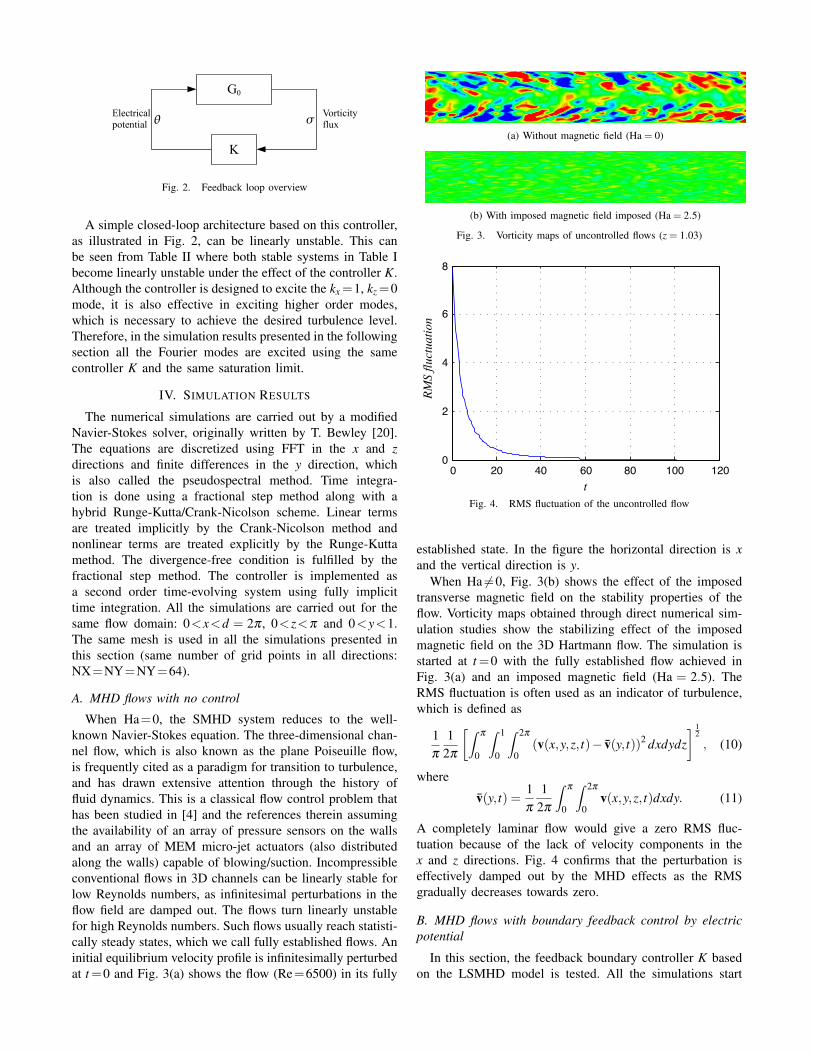
When Ha=0, the SMHD system reduces to the well-known Navier-Stokes equation. The three-dimensional chan-nel flow, which is also known as the plane Poiseuille flow,is frequently cited as a paradigm for transition to turbulence,and has drawn extensive attention through the history offluid dynamics. This is a classical flow control problem thathas been studied in [4] and the references therein assumingthe availability of an array of pressure sensors on the wallsand an array of MEM micro-jet actuators (also distributedalong the walls) capable of blowing/suction. Incompressibleconventional flows in 3D channels can be linearly stable forlow Reynolds numbers, as infinitesimal perturbations in theflow field are damped out. The flows turn linearly unstablefor high Reynolds numbers. Such flows usually reach statisti-cally steady states, which we call fully established flows. Aninitial equilibrium velocity profile is infinitesimally perturbedat t=0 and Fig. 3(a) shows the flow (Re=6500) in its fully

(a) Without magnetic field (Ha = 0)

(b) With imposed magnetic field imposed (Ha = 2.5)

Fig. 3. Vorticity maps of uncontrolled flows (z = 1.03)

0 20 40 60 80 100 1200

2

4

6

8

t

RMS

fluct

uatio

n

Fig. 4. RMS fluctuation of the uncontrolled flow

established state. In the figure the horizontal direction is xand the vertical direction is y.

When Ha �=0, Fig. 3(b) shows the effect of the imposedtransverse magnetic field on the stability properties of theflow. Vorticity maps obtained through direct numerical sim-ulation studies show the stabilizing effect of the imposedmagnetic field on the 3D Hartmann flow. The simulation isstarted at t=0 with the fully established flow achieved inFig. 3(a) and an imposed magnetic field (Ha = 2.5). TheRMS fluctuation is often used as an indicator of turbulence,which is defined as

1π

12π

�� π

0

� 1

0

� 2π

0(v(x,y,z, t)− v(y, t))2 dxdydz

� 12, (10)

where

v(y, t) = 1π

12π

� π

0

� 2π

0v(x,y,z, t)dxdy. (11)

A completely laminar flow would give a zero RMS fluc-tuation because of the lack of velocity components in thex and z directions. Fig. 4 confirms that the perturbation iseffectively damped out by the MHD effects as the RMSgradually decreases towards zero.

B. MHD flows with boundary feedback control by electricpotential

In this section, the feedback boundary controller K basedon the LSMHD model is tested. All the simulations start

(a) t = 0.016

(b) t = 0.3

Fig. 5. Vorticity development (y = 0.0837)

with equilibrium solutions achieved after an external mag-netic field is imposed. Simulations are conducted for theseparameters:

Re = 6500, Q = 1.5, Ha = 2.5,

and the saturation limit on the output of K is set to 0.05.The flow remains linearly stable indefinitely if no boundarycontrol is present. The boundary control is expected to drivethe flow to states with higher RMS fluctuation levels, thusenhancing mixing.

Fig. 5 shows two snapshots of vorticity maps η at afixed y plane at different time instances of the simulation.In the figures the horizontal direction is x and the verticaldirection is z. We can clearly see that the vorticity issignificantly enhanced and complex flow structures occurdue to the boundary control. At a very early stage of thesimulation, the effect of the controller can already be seenin Fig. 5(a) as the small perturbation is introduced by therapidly growing electric potential actuators. The controllersoon reaches saturation on all of the excited modes.

The growth of the vortices, however, does not stop after thecontroller is saturated. This can be seen in the developmentof Reynolds stresses in Fig. 6, which shows the averaged(over the x and z coordinates) profile of one of the Reynoldsstresses, Ruw, in the lower half channel at three different timeinstances. The maximum Reynolds stress occurs very close tothe boundary, which indicates that the penetration of the flowstructures is somehow limited to the boundary regions. Thisis, however, expected because the main effect of the con-troller is on the wall-normal vorticity η = ∂xu−∂xw, whichdoes not involve the wall-normal velocity v. The relation of(6) and (7) determines that the wall-normal velocity is notdirectly controllable in the LSMHD model. The controllerhas to rely on the nonlinear interaction of the wall-normalvorticity to generate wall-normal velocity. The lack of directcontrol over wall-normal velocity limits the penetration of the

−0.2 0 0

0.1

0.2

0.3

0.4

0.5

Ruw

y

−0.2 0 Ruw

−0.2 0 Ruw

Fig. 6. Ruw profiles (t=0.08, 0.24, 2)

0 0.5 1 1.5 2−0.4

−0.3

−0.2

−0.1

0

0.1

t

Reyn

old

Stre

ssRuvRuwRwv

Fig. 7. Reynolds stress development (y = 0.0122)

vortices. Fig. 7 shows all three Reynolds stresses averagedover the x and z coordinates at the y=0.0122 plane, wherethe peak of Reynolds stress occurs. The domination by theRuw component confirms that the controller is efficient incontrolling the wall-normal vorticity, and has very limitedcontribution to the wall-normal velocity.

The wall-normal velocity and vorticity contour maps ofa statistically steady state at a certain z plane is given byFig. 8. In the maps the horizontal direction is x and thevertical direction is y. We can see that the controller ishighly effective in the generation of intense wall-normalvorticity near the boundaries, while the wall-normal velocityis relatively small because of the lack of direct actuation. Itis evident that a means to enhance the transportation alongthe wall-normal direction is necessary.

The actuation of the controller is visualized by the po-tential contour on a y plane very close to the boundary,as the electric potential is almost identical to the one onthe boundary. As Fig. 9 shows, the controller has a veryrich frequency content, due to the excitation of all Fouriermodes. The RMS fluctuation development (Fig. 10) clearly

0.04

0.04

-0.04

-0.04

0.3

0.3

(a) v - velocity

20

1

-1

-20

1

-1

(b) η - vorticity

Fig. 8. Wall-normal velocity and vorticity (t = 2, z = 1.03)

Fig. 9. Electric potential contour on an x-z plane (t = 0.3, y = 0.00837)

shows that the overall turbulence level of an initially stableMHD flow is increased by the feedback control to a level4.6 times higher than that corresponding to an uncontrolledfully developed pure hydrodynamic flow (characterized bythe initial RMS fluctuation value in Fig. 4).

V. CONCLUSION

We propose a boundary controller based on electric po-tential actuation for mixing enhancement in a 3D MHDchannel flow. The controller is based on a linearized SMHDmodel which is discretized by spectral methods. Simultane-ous excitation of all the modes is crucial for the successof the controller. A simple second-order feedback controlis proved to be able to destabilize the vorticity field. Asimple saturation limit is imposed on the actuator to boundthe growth driven by the destabilizing controller. In thisway the system can remain turbulent and bounded. The3D SMHD simulation study confirms the effectiveness ofthe controller by showing increases in the RMS fluctuationand Reynolds stress levels of the otherwise linearly stableflow, thus increasing mixing effects inside the channel. Thesimulation also reveals that the wall-normal penetration ofthe generated turbulence is limited.

Future work includes further study of the destabilizingmechanism of the controller with the ultimate goal of en-hancing wall-normal penetration. The simultaneous controlof wall-normal vorticity using electric potential actuation andof wall-normal velocity using mechanical actuation (blowingand suction) appears as promising.

0 0.5 1 1.5 20

10

20

30

40

50

t

RMS

fluct

uatio

n

Fig. 10. RMS fluctuation of controlled flow

REFERENCES

[1] U. Müller and L. Bühler, Magnetofluiddynamics in Channels andContainers. Springer, 2001.

[2] M. D. Gunzburger, Flow Control, ser. The IMA Volumes in Mathemat-ics and its Applications. New York: Springer-Verlag, 1995, vol. 68.

[3] S. S. Sritharan, Ed., Optimal Control of Viscous Flow. SIAM,Philadelphia, 1998.

[4] O. M. Aamo and M. Krstic, Flow Control by Feedback. Springer,2002.

[5] M. R. Jovanovic, “Turbulence suppression in channel flows by smallamplitude transverse wall oscillations,” Physics of Fluids, vol. 20,no. 1, p. 014101, 2008.

[6] A. B. Tsinober, Viscous Drag Reduction in Boundary Layers, ser.Progress in Astronautics and Aeronautics. Washington, DC: AIAA,1990, no. 123, ch. MHD flow drag reduction, pp. 327–349.

[7] H. Choi, P. Moin, and J. Kim, “Active turbulence control for dragreduction in wall-bounded flows,” J.Fluid Mech., vol. 262, p. 75, 1994.

[8] C. Henoch and J. Stace, “Experimental investigation of a salt waterturbulent boundary layer modified by an applied streamwise magneto-hydrodynamic body force,” Physics of Fluids, vol. 7, no. 6, pp. 1371–1383, June 1995.

[9] T. Berger, J. Kim, C. Lee, and J. Lim, “Turbulent boundary layercontrol utilizing the Lorentz force,” Physics of Fluids, vol. 12, p. 631,2000.

[10] E. Spong, J. Reizes, and E. Leonardi, “Efficiency improvements ofelectromagnetic flow control,” Heat and Fluid Flow, vol. 26, pp. 635–655, 2005.

[11] E. Schuster, L. Luo, and M. Krstic, “MHD channel flow control in2D: Mixing enhancement by boundary feedback,” Automatica, vol. 44,no. 10, pp. 2498–2507, 2008.

[12] L. Luo and E. Schuster, “Heat transfer enhancement in 2D mag-netohydrodynamic channel flow by boundary feedback control,” inProceedings of 45th IEEE Conference on Decision and Control, SanDiego, 2006, pp. 5317–5322.

[13] ——, “Boundary feedback control for heat exchange enhancementin 2D magnetohydrodynamic channel flow by extremum seeking,” inProceedings of the 48th IEEE Conference on Decision and Control,Shanghai, China, December 2009.

[14] J. Hartmann, Theory of the Laminar Flow of an Electrically Conduc-tive Liquid in a Homogeneous Magnetic Field, xv(6) ed. Det Kgl.Danske Vidensk-abernes Selskab Mathematisk-fysiske Meddelelser.

[15] G. Branover, Magnetohydrodynamic Flow in Ducts. Halsted Press,1979.

[16] P. J. Schmid and D. S. Henningson, Stability and Transition in ShearFlows. New York: Springer, 2001, vol. 142.

[17] J. A. C. Weideman and S. C. Reddy, “A MATLAB differentiationmatrix suite,” ACM Transactions on Mathematical Software, vol. 26,no. 4, pp. 465–519, December 2000.

[18] G. H. Cottet and P. D. Koumoutsakos, Vortex Methods: Theory andPractice. Cambridge university press, 2000.

[19] R. L. Panton, Incompressible flow, 2nd ed. New York: Wiley, 1996.[20] T. R. Bewley, Optimal and Robust Control and Estimation of Transi-

tion, Convection, and Turbulence. Stanford University thesis, 1999.