Mixed Models - Worcester Polytechnic Institute · Mixed Models Introduction The Mixed Models task provides facilities for ﬁtting a number of ba-sic mixed models. These models enable

Chapter 15Mixed Models

Chapter Table of Contents

Introduction . . . . . . . . . . . . . . . . . . . . . . . . . . 309

Split Plot Experiment . . . . . . . . . . . . . . . . . . . . . 311

Clustered Data . . . . . . . . . . . . . . . . . . . . . . . . . 320

References. . . . . . . . . . . . . . . . . . . . . . . . . . . . 326

308 � Chapter 15. Mixed Models

SAS OnlineDoc: Version 8

Chapter 15Mixed Models

Introduction

The Mixed Models task provides facilities for fitting a number of ba-sic mixed models. These models enable you to handle both fixed ef-fects and random effects in a linear model for a continuous response.Numerous experimental designs produce data for which mixed mod-els are appropriate, including split-plot experiments, multilocationtrials, and hierarchical designs.

Figure 15.1. Mixed Models Menu

A standard linear model is designed to handlefixed effects, in whichthe levels of the factor represent all possible levels for that factor orat least all levels about which inference is to be made. Factor effectsarerandom effectsif the levels of the factor in a study or experimentare randomly selected from a population of possible levels of thatfactor. The population of possible levels of a random effect has aprobability distribution with a mean and a variance. By modelingboth fixed and random effects, the mixed model provides you with


the flexibility of modeling not only means (as in the standard linearmodel) but variances and covariances as well.

The mixed model is written

y = X� + Z + �

wherey denotes the vector of observed values,X is the known fixedeffects design matrix, and� is the unknown fixed effects parametervector.Z represents the additional random component of the mixedmodel. Here,Z is the known random effects design matrix and is avector of unknown random-effects parameters.Z contains indicatorvariables constructed from the random effects, just asX containsvariables constructed for fixed effects. Finally,� is the unobservedvector of independent and identically distributed Gaussian randomerrors.

Assume that and� are Gaussian random variables that are uncorre-lated and have expectations 0 and variancesG andR, respectively.

E

�

�

�=

�0

0

�

Var

�

�

�=

�G 0

0 R

�

The variance ofy is thereforeV = ZGZ0 +R.

Note that this is a general specification of the mixed model. TheMixed Models task enables you to specify classification random ef-fects that are a special case of the general specification. You canspecify thatZ contains dummy variables,G contains variance com-ponents in a diagonal structure, andR = �2In, whereIn denotesthen� n identity matrix.

The Mixed Models task enables you to specify a mixed model thatincorporates fixed effects and random classification effects and in-cludes interactions and nested terms. You can select from six es-


Split Plot Experiment � 311

timation methods, including maximum likelihood, restricted max-imum likelihood (REML), and MIVQUE. You can also computeleast-squares means, produce Type 1, 2, and 3 tests for fixed ef-fects, and output predicted values and means to a SAS data set. Plotsinclude means plots for fixed effects, predicted plots, and residualplots.

The examples in this chapter demonstrate how you can use the MixedModels task in the Analyst Application to analyze linear models datathat contain fixed and random effects.

Split Plot ExperimentOne of the most common mixed models is the split-plot design. Thesplit-plot design involves two experimental factors, A and B. Levelsof A are randomly assigned to whole plots (main plots), and levels ofB are randomly assigned to split plots (subplots) within each wholeplot. The subplots are assumed to be nested within the whole plotsso that a whole plot consists of a cluster of subplots and a level ofA is applied to the entire cluster. The design provides more preciseinformation about B than about A, and it often arises when A can beapplied only to large experimental units.

The hypothetical data set analyzed in this example was created as abalanced split-plot design with the whole plots arranged in a random-ized complete-block design (Stroup 1989). The response variableYrepresents crop growth measurements. The variableA is a whole plotfactor that represents irrigation levels for large plots, and the subplotvariableB represents different crop varieties planted in each largeplot. The levels ofB are randomly assigned to split plots (subplots)within each whole plot. The data setSplit contains the whole plotfactorA, split plot factorB, responseY, and blocking factorBlock.Using the Mixed Models task, you can estimate variance componentsfor Block, A*Block, and the residual and automatically incorporatecorrect error terms into the tests for fixed effects.



Open the Split Data SetThese data are provided as theSplit data set in the Analyst SampleLibrary. To open theSplit data set, follow these steps:

1. SelectTools! Sample Data: : :

2. SelectSplit.

3. Click OK to create the sample data set in yourSasuser di-rectory.

4. SelectFile! Open By SAS Name: : :

5. SelectSasuser from the list ofLibraries .

6. SelectSplit from the list of members.

7. Click OK to bring theSplit data set into the data table.

Request the Mixed Models AnalysisTo specify the split plot analysis, follow these steps:

1. SelectStatistics! ANOVA ! Mixed Models : : :

2. SelectY as the dependent variable.

3. SelectA, B, andBlock as classification variables.

Figure 15.2. Mixed Models Dialog



Figure 15.2 displays the dialog withY specified as the dependentvariable andA, B, andBlock specified as classification effects in themixed model.

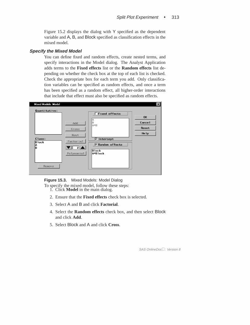
Specify the Mixed ModelYou can define fixed and random effects, create nested terms, andspecify interactions in the Model dialog. The Analyst Applicationadds terms to theFixed effects list or theRandom effectslist de-pending on whether the check box at the top of each list is checked.Check the appropriate box for each term you add. Only classifica-tion variables can be specified as random effects, and once a termhas been specified as a random effect, all higher-order interactionsthat include that effect must also be specified as random effects.

Figure 15.3. Mixed Models: Model DialogTo specify the mixed model, follow these steps:

1. Click Model in the main dialog.

2. Ensure that theFixed effectscheck box is selected.

3. SelectA andB and clickFactorial.

4. Select theRandom effectscheck box, and then selectBlockand clickAdd.

5. SelectBlock andA and clickCross.



These selections create a factorial structure that contains theA andB main effects and theA*B interaction as fixed effects, andBlockand A*Block as random effects. Since you specified the randomeffects, the columns of the model matrixZ now consist of indicatorvariables corresponding to the levels ofBlock andA*Block. TheGmatrix is diagonal and contains the variance components ofBlockand A*Block; the R matrix is also diagonal and contains residualvariance.

Produce Least-Squares MeansYou can request generalized least-squares means of fixed effects us-ing the Means dialog. The least-squares means are estimators of theclass or subclass marginal means that are expected for a balanceddesign. Each least-squares mean is computed asL�̂, whereL isthe coefficient matrix associated with the least-squares mean and�̂

is the estimate of the fixed-effects parameter vector. Least-squaresmeans can be computed for any fixed effect that is composed of onlyclassification variables.

For this analysis, interest lies in comparing response means acrosscombinations of the levels ofA and B. To request least-squaresmeans of theA*B interaction, follow these steps:

1. Click Means in the main dialog.

2. SelectA*B in the candidate list and clickLS Mean.



Figure 15.4. Mixed Models: Means Dialog

When you have completed your selections, clickOK in the maindialog to perform the analysis.

Review the ResultsThe results are presented in the project tree under theMixed Modelsfolder, as displayed in Figure 15.5. The two nodes represent themixed models results and the SAS programming statements (labeledCode) that generate the output.



Figure 15.5. Mixed Models: Project Tree

Double-click on theAnalysis node in the project tree to view thecontents in a separate window.



Figure 15.6. Mixed Models: Model Information

Figure 15.6 displays class level information, dimensions of modelmatrices, and the iteration history of the estimated model. The“Class Level Information” table lists the levels of all classificationvariables included in the model. The “Dimensions” table includesthe number of estimated covariance parameters as well as the num-ber of columns in theX andZ design matrices.

The Mixed Models task estimates the variance components forBlock, A*Block, and the residual by a method known as residual(restricted) maximum likelihood (REML). The REML estimates arethe values that maximize the likelihood of a set of linearly indepen-dent error contrasts, and they provide a correction for the downwardbias found in the usual maximum likelihood estimates.



The “Iteration History” table records the steps of the REML opti-mization process. The objective function of the process is�2 timesthe restricted likelihood. The Mixed Models task attempts to min-imize this objective function via the Newton-Raphson algorithm,which uses the first and second derivatives of the objective functionto iteratively find its minimum. For this example, only one iterationis required to obtain the estimates. The Evaluations column revealsthat the restricted likelihood is evaluated once for each iteration, andthe criterion of 0 indicates that the Newton-Raphson algorithm hasconverged.

Figure 15.7. Mixed Models: Covariance Estimates and Tests forFixed Effects

Figure 15.4 displays covariance parameter estimates, information onthe model fit, and Type 3 tests of fixed effects. The REML estimatesfor the variance components ofBlock, A*Block, and the residual are62.4, 15.4, and 9.4, respectively. The “Fit Statistics” table lists sev-



eral pieces of information about the fitted mixed model: the residuallog likelihood, Akaike’s and Schwarz’s criteria, and the�2 residuallog likelihood. Akaike’s and Schwarz’s criteria can be used to com-pare different models; models with larger values for these criteria arepreferred.

The tests of fixed effects are produced using Type 3 estimable func-tions. The test for theA*B interaction has ap-value of0:0566, indi-cating that there is moderate evidence of an interaction between cropvarieties and irrigation levels.

Figure 15.8. Mixed Models: Least Squares Means

Figure 15.8 displays the least-squares means for each combination ofirrigation levels (A) and crop varieties (B). At each irrigation level,the response is higher for the first crop variety compared to the sec-ond variety. The interaction between crop variety and irrigation lev-els is evident in that variety 1 has a higher mean response than vari-ety 2 at irrigation levels 1 and 2, but the two varieties have nearly thesame mean response at irrigation level 3.



Clustered Data

The example in this section contains information on a study inves-tigating the heights of individuals sampled from different families.The response variableHeight measures the height (in inches) of18 individuals that are classified according toFamily andGender.Since the data occurs in clusters (families), it is very likely that ob-servations from the same family are statistically correlated and notindependent. In this case, it is inappropriate to analyze the data usinga standard linear model.

A simple way to model the correlation is through the use of aFam-ily random effect. TheFamily effect is assumed to be normally dis-tributed with mean of zero and some unknown variance. DefiningFamily as a random effect sets up a common correlation among allobservations having the same level of family.

In addition, a female within a certain family may exhibit more cor-relation with other females in that same family than with the malesin that family, and likewise for males. DefiningFamily*Gender asa random effect models an additional correlation for all observationshaving the same value of bothFamily andGender.

Open the Heights Data SetThese data are provided as theHeights data set in the Analyst Sam-ple Library. To open theHeights data set, follow these steps:

1. SelectTools! Sample Data: : :

2. SelectHeights.

3. Click OK to create the sample data set in yourSasuser di-rectory.

4. SelectFile! Open By SAS Name: : :

5. SelectSasuser from the list ofLibraries .

6. SelectHeights from the list of members.

7. Click OK to bring theHeights data set into the data table.


Clustered Data � 321

Specify the Mixed Models AnalysisTo request a mixed models analysis, follow these steps:

1. SelectStatistics! ANOVA ! Mixed Models : : :

2. SelectHeight as the dependent variable.

3. SelectFamily andGender as classification variables.

4. Click Model to open theModel dialog.

5. Ensure that theFixed effectscheck box is selected.

6. SelectGender and clickAdd.

7. Select theRandom effectscheck box, and then selectFamilyand clickAdd.

8. SelectFamily andGender, and clickCross.

9. Click OK to return to the main dialog.

Based on your selections, the Mixed Models task constructs theX

matrix by creating indicator variables for theGender effect and in-cluding a column of 1s to model the global intercept. TheZ matrixcontains indicator variables for both theFamily effect and theFam-ily*Gender interaction.

Produce a Residual PlotThe Mixed Models task can produce means plots for fixed main ef-fects and interactions, plots of predicted values, and residual plotsthat include or do not include random effects. To produce a plot ofresiduals versus predicted values that includes random effects, fol-low these steps:

1. Click Plots to open thePlots dialog.

2. Click on theResidual tab, and selectPlot residuals vs pre-dicted in theResidual plots (including random effects)box.



Figure 15.9. Mixed Model: Plots Dialog

When you have completed your selections, clickOK in the maindialog to perform the analysis.

Review the ResultsThe results are presented in the project tree under theHeights datain theMixed Models folder, as displayed in Figure 15.10. The threenodes represent the mixed models results, the plot of residuals ver-sus predicted values, and the SAS programming statements (labeledCode) that generate the output.



Figure 15.10. Mixed Models: Project Tree

Double-click on theAnalysis node in the project tree to view thecontents in a separate window.



Figure 15.11. Mixed Models: Analysis Results

Figure 15.11 displays the mixed models analysis results for the clus-teredHeights data. The covariance parameter estimates forFamily,Family*Gender, and the residual variance are 2.4, 1.8, and 2.2, re-spectively. The “Test of Fixed Effects” table contains a significancetest for the single fixed effect,Gender. With a p-value of0:0712,the Type 3 test ofGender is not significant at the� = 0:05 levelof significance. Note that the denominator degrees of freedom forthe Type 3 test are computed using a general Satterthwaite approx-imation. A benefit of performing a random effects analysis usingbothFamily andFamily*Gender as random effects is that you canmake inferences about gender that apply to an entire population offamilies, not necessarily to the specific families in this study.



Figure 15.12. Mixed Models: Residuals Plot

Figure 15.12 displays a plot of the residuals versus predicted valuesthat includes random effects,y �X�̂ � Z ̂ versusX�̂ + Z ̂. Plotsare useful for checking model assumptions and identifying potentialoutlying and influential observations. Based on the plot in Figure15.12, the data seem to exhibit relatively constant variance acrosspredicted values, and there do not appear to be any outliers or influ-ential observations.



References

Littell, R. C., Milliken, G. A., Stroup, W. W., and Wolfinger, R. D.(1996),SAS System for Mixed Models,Cary, NC: SAS InstituteInc.

SAS Institute Inc. (1999),SAS/STAT User’s Guide, Version 7-1,Cary, NC: SAS Institute Inc.

Stroup, W. W. (1989), “Predictable Functions and Prediction Spacein the Mixed Model Procedure,” inApplications of Mixed Mod-els in Agriculture and Related Disciplines,Southern Coopera-tive Series Bulletin No. 343, Louisiana Agricultural ExperimentStation, Baton Rouge, 39–48.


The correct bibliographic citation for this manual is as follows: SAS Institute Inc.,The Analyst Application, First Edition, Cary, NC: SAS Institute Inc., 1999. 476 pp.

The Analyst Application, First EditionCopyright © 1999 SAS Institute Inc., Cary, NC, USA.ISBN 1–58025–446–2All rights reserved. Printed in the United States of America. No part of this publicationmay be reproduced, stored in a retrieval system, or transmitted, by any form or by anymeans, electronic, mechanical, photocopying, or otherwise, without the prior writtenpermission of the publisher, SAS Institute, Inc.U.S. Government Restricted Rights Notice. Use, duplication, or disclosure of thesoftware by the government is subject to restrictions as set forth in FAR 52.227–19Commercial Computer Software-Restricted Rights (June 1987).SAS Institute Inc., SAS Campus Drive, Cary, North Carolina 27513.1st printing, October 1999SAS® and all other SAS Institute Inc. product or service names are registered trademarksor trademarks of SAS Institute Inc. in the USA and other countries.® indicates USAregistration.IBM®, ACF/VTAM®, AIX®, APPN®, MVS/ESA®, OS/2®, OS/390®, VM/ESA®, and VTAM®

are registered trademarks or trademarks of International Business Machines Corporation.® indicates USA registration.Other brand and product names are registered trademarks or trademarks of theirrespective companies.The Institute is a private company devoted to the support and further development of itssoftware and related services.

Documents

Mixed Models - Worcester Polytechnic Institute · Mixed Models Introduction The Mixed Models task provides facilities for ﬁtting a number of ba-sic mixed models. These models enable