Mixed Logit Estimation of the Value of Travel Timeâ€ - DiVA Portal

1

98-08-26VOT2.RTF

Mixed Logit Estimation of the Value of Travel Time†

Staffan Algers

Pål Bergström

Matz Dahlberg‡

Johanna Lindqvist Dillén

Abstract

In this paper we use mixed logit specifications to allow parameters to vary in the populationwhen estimating the value of time for long-distance car travel. Our main conclusion is that theestimated value of time is very sensitive to how the model is specified: we find that it issignificantly lower when the coefficients are assumed to be normally distributed in thepopulation, as compared to the traditional case when they are treated as fixed. In our most richlyparameterised model, we find a median value of time of 57 SEK per hour, with the major part ofthe mass of the value of time distribution closely centred around the median value. Thecorresponding figure when the parameters are treated as fixed is 89 SEK per hour. Furthermore,our finding that the ratio of coefficients in a mixed logit specification differ significantly from theones in a traditional logit specification is contrary to the results obtained by Brownstone & Train(1996) and Train (1997). Whether the ratios will differ or not depends on the model and the datagenerating process at hand.

Keywords: Mixed Logit, Simulation Estimation, Value of Time

JEL Classification: C15, C25, R41

† We thank Per Johansson and seminar participants at the Royal Institute of Technology in Stockholm and at UppsalaUniversity for helpful comments. Financial support from KFB is gratefully acknowledged.‡ Corresponding author: Department of Economics, Uppsala University, PO Box 513, S-75120 Uppsala, Sweden.E-mail: [email protected]. Staffan Algers ([email protected] or [email protected]) and Johanna LindqvistDillén ([email protected]) are at the Royal Institute of Technology in Stockholm and Transek. Pål Bergström([email protected]) is at the Department of Economics, Uppsala University.

2

1. Introduction

When investigating consumers’ choices between different transportation alternatives the value of

time is a central concept. The value of time is calculated as a trade-off ratio between the in-

vehicle time coefficient and the cost coefficient. Usually one trade-off is used for a specific

segment. A common segmentation is trip purpose, especially private trips and business trips.

However, sometimes the segmentation is extended to account for income levels, trip length etc.

Such an approach was also used in the analysis of the Swedish Value of Time study 1994/95. It

may still be of interest to account for the distribution of the value of time, especially in

forecasting. One way to account for the distribution is to specify a model with regressors that

capture the influence of different socio-economic variables and then apply this on the actual

sample (or a more representative sample) all resulting in a sample specific distribution of the

value of time (see Lindqvist Dillén & Algers (1998)). Such a distribution gives us a picture of the

relative importance of the systematic variation in data.

However, the mentioned study, as well as most earlier ones that have estimated the value of

travel time, have adopted the multinomial logit model. Some disadvantages with the multinomial

logit approach is that one has to assume (i) that the coefficients are fixed in the population, (ii)

that the IIA-assumption holds (implying that the odds ratio between two alternatives does not

change by the inclusion (or exclusion) of any other alternative), and (iii) that repeated choices

made by a respondent are independent. In this study we will, using stated preference data, adopt

a mixed logit approach (also called random parameters logit or random coefficients logit) to allow

parameters to vary in the population when estimating the value of time for long-distance car

travel. By using a mixed logit approach, we do not have to assume that (i)-(iii) are fulfilled. Of

particular interest in this study is to estimate distribution parameters of the coefficients and to

investigate how the value of travel time is affected by allowing the parameters to vary in the

population.

Our main conclusion is that the estimated value of time is very sensitive to how the model is

specified: we find that it is significantly lower when the coefficients are assumed to be normally

distributed in the population, as compared to the traditional case when they are treated as fixed.

We also get significantly better model specifications (better fit to the data) when we allow the

parameters to vary in the population. The finding that the ratio of coefficients in a mixed logit

3

specification differ significantly from the ones in a traditional logit specification is contrary to the

results obtained by Brownstone & Train (1996) and Train (1997). Our conclusion is that whether

the ratios will differ or not depends on the model and the data generating process at hand.

Finally, when we allowed the parameters to vary log-normally in the population, we found that

the models did not converge unless we constrained the dispersion parameter of the log-normal

distribution. This pattern was also observed by Brownstone & Train (1996), and their solution

was to constrain the dispersion parameter to be 0.8326. We also tried that solution but found,

when we tested different restrictions on the dispersion parameter to investigate how the

estimated value of time was affected, that it was very sensitive to the imposed restriction.

The paper is organised as follows: section 2 discusses the theoretical model, section 3 discusses

the econometric method, section 4 describes the data, section 5 presents the results, and section 6

concludes.

2. Theoretical Framework

Linear random utility models are widely used when dealing with the value of time estimated on

revealed preference data. One reason for this is that the correlation between first and second

order terms (including higher order terms) can be quite high and make it impossible to estimate

separate coefficients. Linearity is though a strong assumption in estimation of the value of time

and may hence be inadequate. As we deal with stated preference data which, in contrast to

revealed preference data, is based upon a less correlated design, a non-linear functional form will

be developed and analysed. In our theoretical model, we will follow the standard set-up used in

the literature (see, e.g., Train & McFadden (1978) and Hultkrantz & Mortazavi (1998)).

Assume that the utility function for an individual i is defined by Ui (G, L, S), where G is private

consumption, L is leisure, and S is socio-economic status of the individual. We let the individual

maximise utility subject to money and time constraints:

max Ui (G, L, S)s.t.G + cij = E + wWL = T - W - tij

j ∈ M

G - consumption

4

S - socio-economic statuscj - travel cost for alternative jw - wage rate, givenW - number of hours workedE - exogenous income, givenL - leisuretj - in-vehicle time for alternative jT - total amount of time, given

In words, the first constraint implies that the expenditure on consumption, G, and travel cost, cj,

is equal to labour income, wW, and exogenous income, E. The next constraint state that time

spent on leisure, L, is equal to the total amount of time given, T, minus time working, W, and

time travelling, tj. There are M travel alternatives. The individual chooses the travel alternative,

and hence cj and tj, and the number of hours worked so as to maximise utility Ui (G, L, S) subject

to the identities.

Inserting the first order conditions from the maximisation problem as well as the optimal

working time, W* = f (cij, tij, w, E, T), into the direct utility function, Ui(G, L, S), yields the

following indirect utility function:

Vij(cij, tij )= Uij(E+ w f (cij, tij, w, E, T) - cij, T - f (cij, tij, w, E, T) - tij , S)

Let us approximate Vij with a second order Taylor expansion around the reference states c0, t0 and

s0x (which is a socio-economic vector including K characteristics, where ( )x K= 1,... , ) for travel

alternative j ≠ 0 and individual i:

Vij (cij, tij) = ( )c t0 0, + ( ) ( ) ( )c cVc

t tVt

s sVsi i jx x

x

N

x

− + − + −

=∑0 0 0

1

δδ

δδ

δδ +

12

( ) ( ) ( )

( )( ) ( )( ) ( )( )

( )( )

c cVc

t tVt

s sV

s

c c t tV

c tc c s s

Vc s

t t s sV

t s

s s s s

i i jx xx

N

x

i i i jx xx

N

xi jx x

x

N

x

jx x jz zz

N

x

− + − + − +

− − + − − + − − +

− −

=

= =

==

∑

∑ ∑

∑

02

2

2 02

2

2 02

1

2

2

0 0

2

0 01

2

0 01

2

0 011

2

δδ

δδ

δδ

δδδ

δδδ

δδδ

N

x z

Vs s∑

δδδ

2

x≠z

5

When a Taylor expansion to order n is assumed to be sufficiently accurate, then the rest term is

close to zero, why this term is left out. The last equation will form the basis for our empirical

investigation. Since factors that are constant over alternatives cancel out in the probability

expression, we can only identify socio-economic variables when these are interacted with the cost

and/or time variable. Before turning to the actual results we will next discuss the econometric

method to be used.

3. Econometric Method

In this paper we make use of panel data (repeated choices in a stated preference study) with the

decision-makers facing two alternatives in each choice situation.1 A main purpose with the paper

is to estimate distribution parameters for coefficients in a value of time study. To achieve this

goal we will adopt the mixed logit procedure described in Revelt & Train (1997) and Train

(1997).

The fixed coefficient assumption is the traditional one in value of time studies. If we have panel

data, the utility functions typically take the form

U xijt ijt ijt= +β ε'

where i n= 1,..., denotes individual i, j c= 1,..., denotes choice alternative j, t T= 1,...,

denotes time period (or choice situation) t, and εijt is the stochastic part of the utility function.

To give an example by means of a parsimonious value of time model, the deterministic part of

the utility function would take the form β β β' cosx t timeijt ijt ijt= +1 2 .

The common estimation methods in many earlier value of time studies with panel data (at least

with stated preference data) have been bivariate probit and/or bivariate logit. This means that the

likely correlation induced between the choices made by each individual has not been dealt with

appropriately.

1 “Panel data” can be thought of as either revealed preference data where we observe each individual during two ormore time periods or as stated preference data where each individual faces repeated choices.

6

The most common estimation method with multiple alternatives is the multinomial logit (MNL)

method as developed and described by McFadden (1973, 1978). A disadvantage with the MNL

model is that it relies on the IIA property, implying that the odds ratio between two alternatives

does not change by the inclusion (or exclusion) of any other alternative. The IIA property follows

from the assumption that the extreme value distributed residuals are independent over utilities.

An obvious (theoretical) way to handle the IIA property is to allow the unobserved part of the

utility function to be correlated over alternatives by means of a multinomial probit model or a

mixed logit model. This approach has, however, been less obvious in empirical applications since

multiple integrals then have to be evaluated. The improvements in computer speed and in our

understanding of the use of simulation techniques in estimation have however made other

approaches than the traditional one as viable alternatives.

In this paper we want to relax the assumption that the coefficients are the same for all

individuals. We will call the models within this approach mixed logit models.2 Estimating

distribution parameters for coefficients that vary randomly in the population requires more

demanding estimation techniques than in the traditional model with fixed coefficients. With

panel data, the utility functions take the form

U xijt i ijt ijt= +β ε'

where βi is unobserved for each i; otherwise with the same notation as above. This set-up allows

us, for example, to let the coefficient for the cost and/or time variable in a value of time study to

vary over individuals (following, e.g., a normal or a lognormal distribution).

For a general characterisation in a cross-sectional setting, let βi vary in the population with

density ( )f iβ θ , where θ are the true parameters of the distribution. Furthermore, assume that

εij are iid extreme value distributed. If we knew the value of βi , the conditional probability that

person i chooses alternative j is standard logit:

2 Several names have been used in the literature: random coefficient logit, random parameters logit, mixedmultinomial logit, error components logit, probit with a logit kernel, and mixed logit. These names label the sameunderlying model. We stick, as mentioned, with the name ‘mixed logit’.

7

( )Le

eij i

x

x

j

i ij

i ijβ

β

β=∑

'

' (1)

We do not, however, know the persons’ individual tastes. Therefore, we need to calculate the

unconditional probability, which is obtained by integrating (1) over all possible values of βi :

( ) ( ) ( ) ( )L L f de

ef dij ij i i i

x

x

j

i i

i ij

i ijθ β β θ β β θ β

β

β= =∫ ∑∫

'

' (2)

One study using two alternatives and cross-sectional data is conducted by Ben-Akiva, Bolduc &

Bradley (1993). They allow the value of time parameter to follow a lognormal distribution3, and

use a Gaussian quadrature to evaluate the integral.4 However, using quadratures becomes less

attractive the larger the dimension of the integrals we have to evaluate (see, e.g., Press et al.

(1992)). Since, in the model described in equations (1) and (2), the dimension of the integrals to

be evaluated increases with the number of coefficients that are allowed to vary in the population,

approaches using Gaussian quadrature to evaluate integrals must be considered being of limited

value. A more fruitful approach is then to use simulation methods. Brownstone & Train (1996)

and Brownstone, Bunch & Train (1997) have considered this, in a cross-sectional setting, through

a mixed logit specification. The model specification in these two papers is identical.

Brownstone & Train (1996) and Brownstone, Bunch & Train (1997) assume that

( )β η ηi ij i ij ij i ijx b x b x x' ' ' '= + = + , where b is the population mean and ηi is the stochastic

deviation which represents the individual’s tastes relative to the average tastes in the population.

This means that the utility function takes the form U b x xij ij i ij ij= + +' 'η ε , where ηi ijx' are error

components that induce heteroskedasticity and correlation over alternatives in the unobserved

portion of the utility. This means that an important implication of the mixed logit specification is

that we do not have to assume that the IIA property holds. Let ( )g iη θ denote the density for

η . Then different patterns of correlation, and hence different substitution patterns, can be

3 Ben-Akiva et al. rewrite their basic model to obtain a model in which one of the parameters is interpreted as a valueof time parameter. The other parameters in their model have degenerate distributions.4 More specifically, they use a Gauss-Hermite quadrature. Several different Gaussian quadratures exist (see, e.g.,Press et al. (1992)).

8

obtained through different specifications of ( )g ⋅ and xij . For some further results for the mixed

logit model, see below.

The version of the mixed logit model described here is not designed for panel data. Revelt &

Train (1997) and Train (1997) have, however, provided such an extension. Next we turn to these

models.

The basic set-up in Revelt & Train (1997) and Train (1997) is the same as the one outlined above.

The major difference is that a subscript t enters into equations (1) and (2) and into the utility

function, which now takes the form U b x xijt ijt i ijt ijt= + +' 'η ε . However, since we have panel

data, we need an expression for the probability to observe each sampled person’s sequence of

observed choices. Conditional on ηi , the probability of i’s observed sequence of choices is the

product of standard logits:

( ) ( )( )S Li i ij i t it

η η= ∏ ,

where ( )j i t, denotes the alternative that person i chooses in period t.

The unconditional probability for the sequence of choices is then:

( ) ( ) ( ) ( )( ) ( )S S f d L f di i i i i ij i t i i it

θ η η θ η η η θ η= = ∏∫∫ , (3)

Since the integral in (3) cannot be evaluated analytically, exact maximum likelihood estimation is

not possible. Instead the probability is approximated through simulation. Maximisation is then

conducted on the simulated log-likelihood function.5 The algorithm we use to obtain the

5 The mixed logit approach as described here has been used in some applications. Examples include Brownstone &Train (1996) (households’ choices among gas, methanol, electric, and CNG vehicles; stated preference data),Brownstone, Bunch & Train (1997) (households’ choices among gas, methanol, electric, and CNG vehicles; statedand revealed preference data), Revelt & Train (1997) (households’ choices of appliance efficiency level; statedpreference data), and Train (1997) (anglers’ choice of fishing site; revealed preference data). As far as we know, nostudy estimating value of travel time has so far employed a mixed logit specification in the general way describedhere.

9

simulated maximum likelihood results can somewhat heuristically be described as follows (for

further details see, e.g., Brownstone & Train (1996) and Revelt & Train (1997))6:

i) Set starting values for the distribution of the coefficient of interest, say β, i.e. in case of a

normally distributed coefficient, the mean and the variance, say b and η.

ii) Draw a random individually specific coefficient βi from this distribution for each person. This

coefficient is kept constant for the individual through all of his/her responses. The random

coefficients are, still assuming normally distributed coefficients, distributed as β∼NID(b , η)

iii) Use data and the obtained random coefficients to evaluate the likelihood function in a

standard fashion, i.e. treating the random coefficients as if they were fixed.

iv) Repeat steps ii) and iii) r times, thus obtaining r values for the likelihood function il .

v) Compute the average r

r

ii∑

=1

l, which is our simulated value for the likelihood.

vi) Change b and η and repeat steps ii) - v) until we have found a maximum. The values of b and

η are then our simulated maximum likelihood estimates.

Compared to the panel data model with degenerate distributions for the coefficients, the

specification in (3) has (at least) two advantages: it does not exhibit the restrictive IIA property

and it accounts explicitly for correlations in unobserved utility over time or over repeated choices

by each individual.

An alternative to the mixed logit model described above is the multinomial probit model, which

might allow for correlations over alternatives and time (or repeated choices). There are however 6 The estimation method proposed and used for mixed logit models in earlier studies is the maximum simulatedlikelihood (MSL). According to Stern (1997), the MSL is one of four existing simulation based estimation methods.The other three are the method of simulated moments (MSM), the method of simulated scores (MSS), and theMonte Carlo Markov Chain (MCMC) method (where one of the most known MCMC methods is Gibbs sampling).The most common methods are MSL and MSM, with some advantages for MSL (see Börsch-Supan & Hajivassiliou(1993) and Hajivassiliou, McFadden & Ruud (1996)). According to Stern, MSS is the least developed of the four, butit holds some significant promise. There are mixed evidence regarding the properties of Gibbs sampling methods(see Stern (1997)). It is left for future research to decide if any of the less developed methods is to be preferred over

10

some results in the literature indicating that the mixed logit model might be preferable in

situations where the aim is to estimate distribution coefficients for parameters in a model. These

and other results will be discussed in the rest of this section.

McFadden & Train (1996) establish, among other results, the following:7 (1) Under mild

regularity conditions, any discrete choice model derived from random utility maximisation has

choice probabilities that can be approximated as closely as one pleases by a mixed logit model,

(2) A mixed logit model with normally distributed coefficients can approximate a multinomial

probit model as closely as one pleases, and (3) Non-parametric estimation of a random utility

model for choice can be approached by successive approximations by mixed logit models with

finite mixing distributions; e.g., latent class models. From an economic point of view, result (1) is

interesting since we often want to put a utility maximising perspective on the problem at hand.

Furthermore, if we want to make welfare analysis (e.g., calculate willingness to pay), it is crucial

that the observed choice probabilities can be motivated as the outcome of a utility maximisation

problem. If not, welfare analysis cannot be conducted. Result (2) is useful since it implies that

mixed logit can be used wherever multinomial probit has been suggested and/or used. Additional

evidence on this point is given by Ben-Akiva & Bolduc (1996) (as reported by McFadden (1996))

and by Brownstone and Train (1996). Ben-Akiva & Bolduc (1996) find in Monte Carlo

experiments that the mixed logit model gives approximation to multinomial probit probabilities

that are comparable to the Geweke-Hajivassiliou-Keane simulator. Brownstone and Train (1996)

find in an application that the mixed logit model can approximate multinomial probit

probabilities more accurately than a direct Geweke-Hajivassiliou-Keane simulator, when both are

constrained to use the same amount of computer time.

Advantages with the mixed logit specification does then include:

i) The model does not exhibit the IIA property.

ii) The model accounts for potential correlation over repeated choices made by each individual.

iii) The model can be derived from utility maximising behaviour.

iv) The model can, as closely as one wishes, approximate multinomial probit models.

v) Unlike pure probits, mixed logits can represent situations where the coefficients follow other

distributions than the normal. Furthermore, as results in Revelt & Train (1996) and

the MSL method. For introductory and survey literature on simulation estimation, see Hajivassiliou & Ruud (1994),McFadden & Ruud (1994), Gouriéroux & Monfort (1996), and Stern (1997).7 These results are obtained from McFadden (1996).

11

Brownstone and Train (1996) show, when using the estimates for forecasting one may obtain

counter-intuitive and unrealistic results by imposing a normal distribution on some

coefficients. By their very nature, pure probits are sensitive to this problem. For further

discussion on this topic, see, e.g., Brownstone and Train (1996, p. 12f).

vi) If the dimension of the mixing distribution is less than the number of alternatives, the mixed

logit might have an advantage over the multinomial probit model simply because the

simulation is over fewer dimensions.

4. Data

The data used in this study is part of the 1994 Swedish Value of Time study. When this study was

initiated, it was decided to concentrate on regional and long distance trips, since they would be

the most important trip types in the evaluation work, and since some information already existed

for local trips. Information was collected for private as well as for business trips for six different

modes; car, air, long distance train, regional train, long distance bus and regional bus.

The study was based on stated preference data and was ambitiously prepared. The main study

was preceded by several pilot studies and international expertise was involved in the work.

The study was designed as a telephone survey, in which socio-economic information of the

respondent and her household, information related to business trips and responses to stated

preference experiments was collected.

The principle for the fieldwork was first to contact a person during a trip, in order to give the

stated preference experiment a realistic context, and then to make the interview by telephone on

the agreed day. However, for the car mode, which is the mode we focus on in this paper, this

meant that license plate numbers were noted at selected road sections, and then the car owners

were contacted and asked for the person who drove the car at the specific time and location.

The sample size (comprising private values for private and business trips) contained about 850

car interviews. The response rate for the car interviews was about 65 percent.

12

The stated preference experiment was designed so that the respondent was presented one base

alternative and a change from this alternative. This had the advantage that the design did not

contain dominant alternatives, which could make the respondents annoyed if included and could

cause estimation problems if excluded. A drawback might however be that it makes it easier for

the respondents to escape to a “no change” choice. To reduce this problem, the reported data on

actual time and cost was randomly multiplied by 0.9 or 1.1, so that the base alternative would not

appear to be exactly the same. The base alternative was also referred to as the “C” alternative,

which was to be compared to A, B, D, E etc.

To give information on the value of time losses as well as time savings, changes representing

gains and losses were presented equally often (four times each in each game). The first choices

were randomly gains or losses, to avoid bias depending on the initial question.

In this study we restrict the analysis to one of the segments that we dealt with in 1994/95, namely

private car trips over 50 kilometres. Furthermore, we only use those individuals who have eight

fulfilled choices, leaving us with a sample of 2024 observations.

5. Results

Brownstone & Train (1996) and Train (1997) find that ratios of their estimated coefficients in a

mixed logit specification are similar to those estimated in a traditional logit specification.

Brownstone & Train (1996) then conclude that “If indeed the ratios of coefficients are

adequately captured by a standard logit model, ... , then the extra difficulty of estimating a mixed

logit or a probit need not be incurred when the goal is simply estimation of willingness to pay,

without using the model for forecasting.”. Since our goal is “simply to estimate willingness to

pay”, we will start out by investigating if the ratios of coefficients (i.e. the value of time) are

unaffected by the model specification also in our case. In doing this, we estimate a parsimonious

model in which we only have cost (COST), in-vehicle time (TIME), and an alternative-specific

constant for the base alternative which we will refer to as an inertia coefficient (INERTIA) as

explanatory variables. Using the data described in the former section, we have estimated all eight

possible combinations of normal and fixed parameters for the three coefficients mentioned

above. The estimation was carried out on the entire sample as well as the sub-samples where

individuals were offered only a shorter in-vehicle time at a higher cost (the willingness to pay,

13

WTP, sample) and where they were offered only a longer in-vehicle time at a discount (the

willingness to accept, WTA, sample). The computed values of time for all of these models are

given in Table 18, whereas the corresponding log-likelihood values are given in Table 2. The

entire estimation output is included as Appendix A. In all estimations we used 1000 replications

(i.e., r = 1000) to calculate the simulated likelihood function.9

Table 1. Value of time (SEK/h).

Model WTA WTP Pooled CTI

1 117.04

(9.00)

102.19

(12.00)

92.41

(6.00)

FFF

2 137.94

(12.60)

93.33

(12.00)

85.25

(6.60)

FNF

3 112.53

(10.20)

87.67

(10.20)

91.81

(4.80)

FFN

4 76.26

(17.40)

28.27

(4.80)

51.32

(5.40)

NFF

5 95.35

(13.20)

60.44

(10.80)

59.73

(5.40)

NNF

6 83.01

(12.60)

51.35

(8.40)

47.87

(4.80)

NFN

7 132.90

(12.60)

97.20

(12.00)

82.58

(6.60)

FNN

8 99.00

(14.40)

56.58

(7.20)

55.98

(4.80)

NNN

Notes: The number of each model corresponds to those of

Appendix A. Values of time are given in SEK per hour. Values in

parentheses are standard errors. The column CTI (Cost Time

Inertia) indicates which of the coefficients that have been treated as

Fix or Normally distributed.

8 The estimated value of time (per minute) is obtained by dividing the estimated marginal utility of time with theestimated marginal utility of cost. For the parsimonious model given here, this is simply TIME/COST. In calculatingstandard errors for the estimated value of time, we have used the Delta method.9 All estimations have been conducted by a GAUSS program written by Kenneth Train, David Revelt, and PaulRuud. The program is available at http://elsa.Berkeley.EDU/~train/

14

The most striking result is that the value of time appears quite sensitive to the assumptions we

make on the coefficients. Adopting a standard logit model by assuming fixed coefficients (model

1) or, to put it differently, ignoring individual heterogeneity, appears to lead to systematically

higher values of time. Specifically, assuming a fixed cost coefficient yields a considerably higher

value of time. Looking at the log-likelihood values in Table 2, it also appears that the assumptions

of fixed coefficients are by no means “innocent” ones. Comparing with the least restricted model

(model 8), where all coefficients are assumed to be normally distributed, no restrictions are

accepted using a likelihood ratio test. Model 5 is the model that is closest to be accepted, but only

for the WTA and WTP sub-samples. For the pooled sample, none of the other models would be

accepted in favour of model 8. Returning to the values of time, a rather odd feature is that the

values for the pooled model do not appear to be averages of the two sub-samples. A natural

suspicion is that this is due to the fact that we have imposed the restriction that the Inertia

parameter should be equal for WTA and WTP observations in the pooled sample; a restriction

not supported by the estimation results for the sub-samples (see Appendix A)10. This could also

be an explanation as to why the restriction of a fixed inertia coefficient is rejected for the pooled

sample. In order to investigate this, we have also estimated the pooled sample with separate

WTA and WTP inertia-parameters. Estimating all 16 models that the additional coefficient would

give rise to if treated as above, is hardly meaningful. We have therefore estimated the least

(NNNN) and the most (FFFF) restricted models, as well as versions of model 5, which was the

one that gave rise to the most plausible alternative specification above. The results can be seen in

Table 3.

Table 2. Log-likelihood values.

WTA WTP Pooled CTI

1 -547.94 -633.54 -1191.99 FFF

2 -483.02 -522.52 -1077.16 FNF

3 -484.62 -527.51 -1169.04 FFN

4 -485.61 -560.03 -1091.14 NFF

5 -468.97 -499.96 -1031.83 NNF

6 -471.72 -515.25 -1032.24 NFN

7 -476.08 -515.95 -1024.82 FNN

8 -465.66 -494.02 - 971.52 NNN

10 This result is also in line with the findings in Lindqvist Dillén & Algers (1998).

15

Table 3. Separate inertia parameters.

Model

CTIWTPIWTA

Value of

Time

Log L

FFFF 107.66

(7.20)

-1186.57

NNFF 78.54

(10.20)

-1027.36

NNFN 68.86

(7.80)

-983.00

NNNF 74.65

(9.00)

-968.00

NNNN 77.62

(9.00)

-958.09

Relaxing the assumption that the inertia parameter is identical for the WTA and WTP sub-

samples, provides us with value of time estimates that seem more like an average of those

obtained from the two samples estimated separately. Estimating both inertia parameters as

normal does also cause the log likelihood to increase significantly as compared to the previous

model 8 for the pooled sample. Treating either or both of the inertia parameters as fixed does

however not appear to be a valid restriction, and the model with all four coefficients random and

normal would hence be our preferred specification in this simple setting.

The conclusion from this exercise is hence that the value of time estimates are sensitive to the

assumption that the parameters do not vary in the population. This result contradicts the results

in Brownstone & Train (1996) and Train (1997), implying that whether ratios of coefficients in

mixed logit specifications and standrad logit specifications differ from each other or not, depends

on the model and datagenerating process at hand and must hence be examined in each case.

Second order Taylor series expansion

In order to obtain a somewhat richer specification, we will now estimate an empirical model

motivated by the second order Taylor series expansion of the indirect utility function given in

section 2. This model will contain squares of the cost and time variables, as well as cost and time

16

interacted with some socio-economic variables. These are Age, which is a dummy variable taking

the value 1 if the respondent is aged 45 or older, Punct, a dummy indicating if the respondent

considers punctuality an important feature of the journey undertaken, Work, a dummy indicating

if the journey was a worktrip, Paid, a dummy indicating if the person is gainfully employed, and

finally, Hhinc, a variable indicating to which out of 14 household income classes the respondent

belongs. If a socio-economic variable has been interacted with the cost variable (time variable), it

will have a “C” (“T”) in front of it in Table 4.

Table 4. Estimating the model resulting from a second order Taylor series expansion withsocio-economic interaction terms

Model 1 Model 2 Model 3Variable Estimate Std. Error Estimate Std. Error Estimate Std. Errorcost (mean) -0.09623* 0.02380147 -0.10199* 0.01410378 -0.02889* 0.00629035cost (sd) 0.07570* 0.01329421 0.09445* 0.01897846time (mean) -0.15811* 0.02739691 -0.15119* 0.02352799 -0.06163* 0.00789074time (sd) 0.02368 0.01598253 0.02468 0.01319905Cage (mean) 0.01095 0.01991367 0.01097 0.00588838Cage (sd) 0.00127 0.00924779Cpunct (mean) -0.05861 0.03832919 -0.04917* 0.02066133Cpunct (sd) 0.02548 0.04440426Cwork (mean) -0.27368* 0.07036961 -0.32663* 0.08004169 -0.08956* 0.01942279Cwork (sd) 0.24141* 0.07015764 0.24534* 0.06540797Cpaid (mean) -0.03633 0.02169053 -0.01396* 0.00583043Cpaid (sd) 0.04017 0.02068383Chhinc (mean) 0.00534 0.00388423 0.00156 0.00096581Chhinc (sd) 0.00284 0.00277444Tage (mean) 0.06788* 0.02028730 0.06526* 0.01978550 0.03055* 0.00695130Tage (sd) 0.01391 0.01374937Tpunct (mean) -0.02148 0.03015937 -0.02269 0.01527083Tpunct (sd) 0.00397 0.03417271Twork (mean) -0.15190* 0.05090743 -0.15276* 0.04491958 -0.05356* 0.01543473Twork (sd) 0.12122* 0.06121859 0.09442* 0.04292405Tpaid (mean) -0.06698* 0.02601288 -0.05613* 0.02390065 -0.02442* 0.00646841Tpaid (sd) 0.09928* 0.01724521 0.08358* 0.01625255Thhinc (mean) -0.00954* 0.00368550 -0.00867* 0.00327612 -0.00292* 0.00118176Thhinc (sd) 0.00248 0.00509888dwta (mean) 0.39461 0.28919065 0.49318 0.28977811 0.20481 0.10756544dwta (sd) 1.95318* 0.30595142 1.93781* 0.32722020dwtp (mean) 1.67058* 0.32804356 1.62451* 0.33080340 0.80177* 0.11414634dwtp (sd) 2.58605* 0.34570052 2.50861* 0.36522659Log L -915.94 -925.38 -1099.63Notes:Model 1: All variables follow a normal distribution.Model 2: Model 1 with insignificant parameters restricted to zero.Model 3: All variables are treated as fixed (i.e., traditional logit estimation).* indicates significance at a 5% level

Estimating the model with both quadratic and interaction terms left the former ones insignificant

at all times, and therefore these terms have been omitted in the specification reported in Table

17

411. We have estimated three models; the two latter nested in the first. The first and most general

model includes all interaction terms and treats all coefficients as random and normally distributed

(Model 1). The second model restricts the insignificant parameters of the first to equal zero

(Model 2). That is, in Model 2 we treat the parameters as fixed whenever the standard deviation

parameter is insignificant, and as equal to zero when both the mean and the standard deviation

are insignificant.

Conducting a likelihood ratio test for the restrictions of Model 2 yields a test value of 18.88 with

12 degrees of freedom, implying that we cannot reject the null hypothesis that the coefficients are

jointly zero at a 5% significance level. Model 3 is the standard logit specification that treats all

coefficients as fixed. Performing a likelihood ratio test between models 1 and 3 emphatically

rejects the restrictions imposed. From these tests, Model 2 is the specification to be preferred.

We have also experimented with allowing the coefficients to follow a log-normal distribution.12

However, without restricting the dispersion parameter of the log-normal distribution (σk ), we

have failed to get the models to converge. This pattern was also observed by Brownstone &

Train (1996). Their solution was to mechanically constrain each σk to be 0.8326. We have also

tried that solution and, as a sensitivity analysis, we tested different restrictions on the dispersion

parameter to investigate how the estimated value of time was affected. It turned out that the

value of time was quite sensitive to the imposed restriction. An illustration of this is given in

Table 5 for the WTP-sample. In this example, COST and INERTIA are treated as fixed while

TIME is assumed to follow a log-normal distribution, and we have constrained σ to be (0.4, 0.5,

0.6, 0.7, 0.8, 0.86636) respectively in six different estimations. 0.86636 is the highest value σ can

take for the model to converge. As can be seen from the last column, the value of time is very

sensitive to the imposed restriction: it decreases from 188.41 SEK/hour to 141.88 SEK/hour

when σ is constrained to be 0.4 instead of 0.86636. When allowing COST or INERTIA or some

combination of the parameters to follow a log-normal distribution, the same pattern as in Table 5

occurred. Our conjecture is hence that the log-normal distribution is problematic in the present

context, and we will keep Model 2 in Table 4 as our preferred specification.

11 All estimates including quadratic terms are available upon request.12 The k-th coefficient with a log-normal distribution is specified as ( )exp µ σ υk k k+ , where υk is iid standardnormal and µk and σk are parameters to be estimated.

18

Table 5. Effects on the value of time of constraining the dispersion parameter (σ) in the log-normal distribution. TIME is assumed to be log-normally distributed, while COST and

INERTIA are assumed to be fixed (INERTIA-estimates not reported).TIME (σ) TIME (µ) TIME (mean) COST Value of time

0.86636 -1.56494 -0.30433 -0.09691 188.41

0.8 -1.5585 -0.28982 -0.09672 179.80

0.7 -1.55822 -0.26895 -0.09591 168.26

0.6 -1.58127 -0.24628 -0.09337 158.27

0.5 -1.65153 -0.21729 -0.08725 149.43

0.4 -1.82268 -0.17505 -0.07403 141.88

Looking a bit more closely at Model 2, it appears as if the coefficients have reasonable signs. If

the journey in question is a “work-trip”, utility is affected more negatively than else by both

increased cost and time, which seems plausible since if the journey is repeated on a daily basis,

the cost and time associated to it should reduce utility more than if the journey was just a one

time occasion. It is furthermore worth noting that the variance of Cwork is quite large, which

perhaps could be explained by the fact that several respondents may obtain tax allowances for

work-trips and hence have little or no extra dis-utility from the journey being a work-trip.

Age enters just through the time interaction term and it enters with a positive sign, indicating that

people aged 45 or more seem less sensitive to travel time than do younger respondents. Income,

which probably is correlated with the Paid-dummy, enters significantly and negatively interacted

with time, suggesting that people with higher income get relatively higher dis-utility from the time

spent on their journeys.

The main source of concern in the specification obtained is the rather large variance of the cost-

coefficient. Since our key variable of interest is the value of time, where the cost coefficient is

included in the denominator, there is a relatively large probability of obtaining realisations of this

coefficient equal to or close to zero. This poses a problem in that we are likely to obtain

unrealistic values of time as a direct consequence of the empirical model if the focus is to

estimate the distribution of the value of time. To alleviate this we have tried to let the cost-

coefficient follow a log-normal distribution, however encountering the convergence problems

mentioned earlier. The restriction of treating the cost coefficient as fixed is also emphatically

rejected by a likelihood ratio test.

19

The values of time implied by Model 2 in Table 4 have to be simulated using the data at hand

since these will involve the regressors and become individually specific, once we have allowed for

higher order terms. Due to the problem with potentially extreme observations, there are two

ways of attacking the problem. Either we treat the obtained averages of the estimated coefficients

as fix and evaluate the value of time distribution at these points (which would be in line with

earlier research, see e.g. Lindqvist Dillén & Algers (1998)), or we could use simulation techniques

and assign each individual random coefficients, where the coefficients are drawn from normal

distributions with distribution coefficients given by the estimation results. Even though the

averages of the two methods hardly would be comparable, the much less outlier-sensitive

medians would be a reasonable point of comparison. We will therefore make use of the median

value of time.

Figure 1. Value of time distribution (90% of the mass)Model 2 and value of time distribution calculated when the distribution of the parameters is taken

into account (calculated through simulation).

Notes to Figure 1:5% in each tail has been dropped.Median value of time for whole distribution: 56.98Median value of time for distribution presented in Fig. 1: 56.285th percentile value of time: -187.9195th percentile value of time: 417.16

20

Starting with the estimates obtained in Model 2 and calculating the value of time distribution

when the distribution of the parameters is taken into account, we obtain a median value of time

of 56.98 (see Figure 1). From Figure 1 we can also see that the major part of the mass is in a close

interval around the median value of time. If we still use Model 2, but follow earlier studies and

treat all coefficients as fixed in the calculation of the value of time (i.e., ignoring the estimated

standard deviations of the coefficients in Model 2), we get the distribution given in Figure 2. The

median value of time increases to 74.18. This result can be compared to the distributions

presented so far in the literature, where coefficients have been treated as fixed in both the

estimation and in the calculation of the distribution of the value of time. That is, using the

estimates obtained in Model 3, Figure 3 presents the traditional value of time distribution. In this

set-up, the median value of time has increased even more (to 89.25). This pattern of a decreasing

value of time when the parameters are allowed to vary in the population is in line with the pattern

we observed for the parsimonious model presented in tables 1 and 3.

Figure 2. Value of time distribution Model 2 and value of time distribution calculated with parameters treated as fixed.

Notes to Figure 2:Median value of time: 74.18

21

Figure 3. Value of time distribution Model 3: Parameters treated as fixed in the estimation.

Notes to Figure 3:Median value of time: 89.25

6. Conclusions

In this paper we have used mixed logit specifications to allow parameters to vary in the

population when estimating the value of time for long-distance car travel. Our main conclusion is

that the estimated value of time is very sensitive to how the model is specified: we find that it is

significantly lower when the coefficients are assumed to be normally distributed in the

population, as compared to the traditional case when they are treated as fixed. In our most richly

parameterised model, we find a median value of time of 57 SEK per hour, with the major part of

the mass of the value of time distribution closely centred around the median value. The

corresponding figure when the parameters are treated as fixed is 89 SEK per hour. Furthermore,

we get significantly better model specifications (better fit to the data) when we allow the

parameters to vary in the population.

Our result that the ratio of coefficients in a mixed logit specification differ significantly from the

ones in a traditional logit specification is contrary to the results obtained by Brownstone & Train

(1996) and Train (1997). A second conclusion from this study is hence that whether the ratios

will differ or not depends on the model and the data generating process at hand.

22

Finally, when we allowed the parameters to vary log-normally in the population, we found that

the models did not converge unless we constrained the dispersion parameter of the log-normal

distribution. This pattern was also observed by Brownstone & Train (1996), and their solution

was to mechanically constrain the dispersion parameter to be 0.8326. We also tried that solution

but found, when we tested different restrictions on the dispersion parameter to investigate how

the estimated value of time was affected, that the value of time was very sensitive to the imposed

restriction. An illustration was given in the paper in which it was shown that the value of time

decreased from 188.41 SEK/hour to 141.88 SEK/hour when the dispersion parameter was

constrained to be 0.4 instead of 0.86636 (where 0.86636 was the highest value the dispersion

parameter could take for the model under consideration to converge). A third conclusion from

this paper is then that in certain contexts it might be unwise to impose restrictions on parameters

in the log-normal distribution to get models to converge. Since ratios of coefficients might be

very sensitive to the imposed restrictions, a good idea would be to conduct a sensitivity analysis

for each unique model.

References

Ben-Akiva, M. and D. Bolduc (1996), “Multinomial Probit with a Logit Kernel and a General

Parametric Specification of the Covariance Structure”, Mimeo, MIT.

Ben-Akiva, M., D. Bolduc, and M. Bradley (1993), “Estimation of Travel Choice Models with

Randomly Distributed Values of Time”, Transportation Research Record, 1413, 88-97.

Brownstone, D. and K.E. Train (1996), “Forecasting New Product Penetration with Flexible

Substitution Patterns” , Journal of Econometrics, forthcoming.

Börsch-Supan, A. and V.A. Hajivassiliou (1993), “Smooth Unbiased Multivariate Probability

Simulators for Maximum Likelihood Estimation of Limited Dependent Variable Models”, Journal

of Econometrics, 58, 347-368.

23

Börsch-Supan, A. et al. (1992), “Health, Children, and Elderly Living Arrangements: A

Multiperiod-Multinomial Probit Model with Unobserved Heterogeneity and Autocorrelated

Errors”, in Topics in the Economics of Aging, D. Wise (Ed.), University of Chicago Press, 79-104.

Gouriéroux, C. and A. Monfort (1996), “Simulation-Based Econometric Methods”, CORE

Lectures, Oxford University Press.

Hajivassiliou, V.A. and P. Ruud (1994), "Classical Estimation Methods for LDV Models using

Simulation", in R.F. Engle and D.L. McFadden (eds.), Handbook of Econometrics, Vol. IV,

Amsterdam: North-Holland.

Hajivassiliou, V.A., D. McFadden and P. Ruud (1996), "Simulation of Multivariate Normal

Rectangle Probabilities and Their Derivatives: Theoretical and Computational Results", Journal of

Econometrics, 72, 85-134.

Hultkrantz, L. and R. Mortazavi (1998), “The Value of Travel Time Changes in a Random

Nonlinear Utility Model”, Mimeo, CTS.

Keane, M.P. (1994), “A computationally Practical Simulation Estimator for Panel Data”,

Econometrica, 62, 95-116.

Lindqvist Dillén, J. and S. Algers (1998), “Further Research on the National Swedish Value of

Time Study”, Mimeo, KTH and Transek.

McFadden, D.L. (1973), "Conditional Logit Analysis of Qualitative Choice Behavior," in P.

Zarembka (ed.), Frontiers in Econometrics, 105-142, Academic Press: New York.

McFadden, D.L. (1978), “Modeling the Choice of Residential Location”, in A. Karlqvist et al.

(eds.), Spatial Interaction Theory and Residential Location, 75-96,

Amsterdam, North-Holland.

McFadden, D. (1996), “Lectures on Simulation-Assisted Statistical Inference”, Lectures given at

the 1996 EC-squared Conference, Florence, Italy.

24

McFadden, D.L. and P. Ruud (1994), "Estimation by Simulation", Review of Economics and Statistics,

76, 591-608.

McFadden, D. & K.E. Train (1996), “Mixed MNL Models for Discrete Response”, Mimeo,

Berkeley.

Press, W.H., B.P. Flannery, S.A. Teukolsky, and W.T. Vetterling (1992), Numerical Recipes - The

Art of Scientific Computing, Cambridge University Press, Cambridge.

Revelt, D. and K.E. Train (1997), “Mixed Logit with Repeated Choices: Households’ Choices of

Appliance Efficiency Level”, Review of Economics and Statistics (forthcoming).

Stern, S. (1997), “Simulation-Based Estimation”, Journal of Economic Literature, XXXV, 2006-2039.

Train, K.E. (1997), “Recreation Demand Models with Taste Differences Over People”, Land

Economics (forthcoming).

Train, K. and D. McFadden (1978), “The Goods/Leisure Tradeoff and Disaggregate Work Trip

Mode Choice Models”, Transportation Research, 12, 349-353.

25

Appendix A

Complete estimation results for the models presented in tables 1 and 2.

A1. Pooled sample

Model 1. Standard logit results.Variable Coefficient Std. Error

COST -0.02857132 0.00239913

TIME -0.04400165 0.00266707

INERTIA 0.43500673 0.05038086

Log Likelihood -1191.992

Observations 2024

Value of time* 92.41

(6.00)

* SEK per hour (standard error)

Model 2. TIME normally distributed, COST and INERTIA fixed.Variable Coefficient Std. Error

COST -0.05501511 0.00452735

TIME (mean) -0.07816269 0.00702507

TIME (sd) 0.07029758 0.00725689

INERTIA 0.55742546 0.05987251


Observations 2024


(6.60)


Model 3. INERTIA normally distributed, COST and TIME fixed.Variable Coefficient Std. Error

COST -0.03217808 0.00270026

TIME -0.04923548 0.00304682

INERTIA (mean) 0.49393659 0.07320515

INERTIA (sd) -0.76662098 0.08989499


Observations 2024


(4.80)


26

Model 4. COST normally distributed, TIME and INERTIA fixed.Variable Coefficient Std. Error

COST (mean) -0.07576494 0.00927421

COST (sd) 0.09158090 0.01034064

TIME -0.06480919 0.00410452

INERTIA 0.58272064 0.06062562


Observations 2024


(5.40)


Model 5. COST and TIME normally distributed, INERTIA fixed.Variable Coefficient Std. Error

COST (mean) -0.11189049 0.01274776

COST (sd) 0.10842281 0.01377712

TIME (mean) -0.11139466 0.00987554

TIME (sd) 0.07641951 0.00887209

INERTIA 0.70958592 0.07111969


Observations 2024


(5.40)


Model 6. COST and INERTIA normally distributed, TIME fixed.Variable Coefficient Std. Error

COST(mean) -0.11384950 0.01428848

COST (sd) 0.13289484 0.01473858

TIME -0.09082613 0.00645161

INERTIA (mean) 0.84225080 0.12614201

INERTIA (sd) 1.44748837 0.14931759


Observations 2024


(4.80)


27

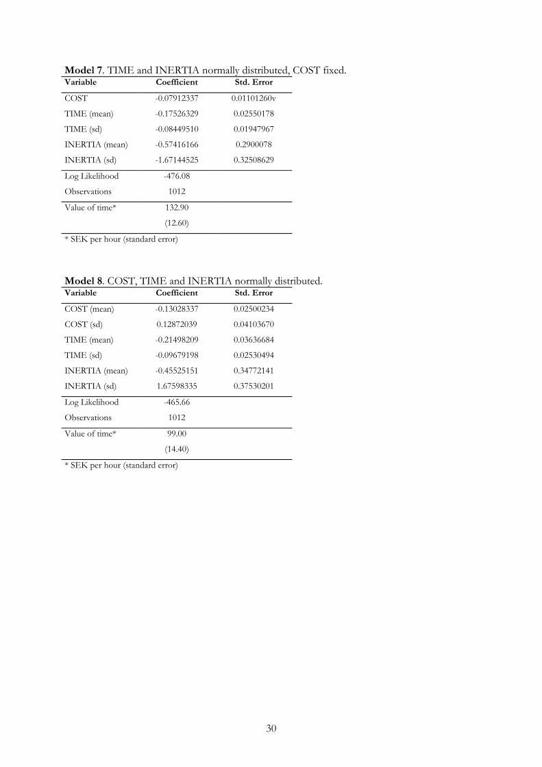
Model 7. TIME and INERTIA normally distributed, COST fixed.Variable Coefficient Std. Error

COST -0.07614540 0.00662259

TIME (mean) -0.10479940 0.01049346

TIME (sd) -0.09857771 0.00999531

INERTIA (mean) 0.78004300 0.12297355

INERTIA (sd) 1.37871864 0.14956621


Observations 2024


(6.60)


Model 8. COST, TIME and INERTIA normally distributed.Variable Coefficient Std. Error

COST (mean) -0.17028816 0.02017033

COST (sd) 0.14253766 0.01707413

TIME (mean) -0.15888294 0.01526542

TIME (sd) 0.10950636 0.01269758

INERTIA (mean) 1.04151591 0.15798329

INERTIA (sd) 1.65744534 0.18695852


Observations 2024


(4.80)


28

A2. WTA sample


COST 0.03480418 0.00366443

TIME 0.06788942 0.00664065

INERTIA 0.03412255 0.12017560


Observations 1012


(9.00)



COST -0.09194979 0.01130053

TIME (mean) -0.21139545 0.02551612

TIME (sd) 0.12718125 0.01687183

INERTIA -0.82132800 0.22385750


Observations 1012


(12.60)



COST -0.05940237 0.00706989

TIME -0.11140799 0.01325713

INERTIA (mean) 0.04103386 0.27101912

INERTIA (sd) -2.29804516 0.27096060


Observations 1012


(10.20)


29


COST (mean) -0.09549830 0.01997407

COST (sd) 0.18550966 0.02718516

TIME -0.12137828 0.01442329

INERTIA 0.10561015 0.21371861


Observations 1012


(17.40)



COST (mean) -0.15304232 0.02676092

COST (sd) 0.18783736 0.03456083

TIME (mean) -0.24320288 0.03658566

TIME (sd) 0.11899159 0.02110499

INERTIA -0.56016455 0.29253645


Observations 1012


(13.20)



COST(mean) -0.09945335 0.01773147

COST (sd) 0.11605056 0.02875754

TIME -0.13758721 0.01736925

INERTIA (mean) 0.04984306 0.30172327

INERTIA (sd) 1.99539453 0.31821491


Observations 1012


(12.60)


30


COST -0.07912337 0.01101260v

TIME (mean) -0.17526329 0.02550178

TIME (sd) -0.08449510 0.01947967

INERTIA (mean) -0.57416166 0.2900078

INERTIA (sd) -1.67144525 0.32508629


Observations 1012


(12.60)



COST (mean) -0.13028337 0.02500234

COST (sd) 0.12872039 0.04103670

TIME (mean) -0.21498209 0.03636684

TIME (sd) -0.09679198 0.02530494

INERTIA (mean) -0.45525151 0.34772141

INERTIA (sd) 1.67598335 0.37530201


Observations 1012


(14.40)


31

A3. WTP sample


COST -0.02535229 0.00352146

TIME -0.04321327 0.00434652

INERTIA 0.56325980 0.11412749


Observations 1012


(12.00)



COST -0.09093669 0.01161694

TIME (mean) -0.14144647 0.01889791

TIME (sd) 0.13860639 0.01722578

INERTIA 1.23266882 0.24313172

Log Likelihood 522.52

Observations 1012


(12.00)



COST -0.06228664 0.00834668

TIME -0.09101428 0.01124031

INERTIA (mean) 1.01065150 0.31731389

INERTIA (sd) 2.84295137 0.31791844


Observations 1012


(10.20)


32


COST (mean) -0.15630464 0.02709515

COST (sd) 0.23348705 0.03977823

TIME -0.07364639 0.00902424

INERTIA 0.04464013 0.21847392


Observations 1012


(4.80)



COST (mean) -0.23171849 0.04764769

COST (sd) 0.19913374 0.04815863

TIME (mean) -0.23342869 0.03543148

TIME (sd) 0.18235746 0.02806683

INERTIA 1.34670766 0.35487931


Observations 1012


(10.80)



COST(mean) -0.13691698 0.02558714

COST (sd) 0.12013089 0.02750179

TIME -0.11718334 0.01593822

INERTIA (mean) 0.83265093 0.39425414

INERTIA (sd) 3.19333965 0.44065746


Observations 1012


(8.40)


33


COST -0.08362443 0.01132617

TIME (mean) -0.13546708 0.01880990

TIME (sd) 0.09358154 0.01666308

INERTIA (mean) 1.36620509 0.31337889

INERTIA (sd) 2.02073803 0.36823448


Observations 1012


(12.00)



COST (mean) -0.23059026 0.04363866

COST (sd) 0.19880449 0.03979997

TIME (mean) -0.21746084 0.03456401

TIME (sd) 0.14470279 0.02781579

INERTIA (mean) 1.41794733 0.40488918

INERTIA (sd) 2.10718854 0.55146506


Observations 1012


(7.20)


Documents

Mixed Logit Estimation of the Value of Travel Timeâ€ - DiVA Portal