Embed Size (px)
Citation preview

Mixed-effects modelsSolutions to Exercises
May 1, 2018

Contents
1 Mixed-effects models 21.10 Exercises . . . . . . . . . . . . . . . . . . . . . . . . . . . . . . . . . . . . . . . . . . . . . . . . . . . . 21.10.1 PREF Canopy data . . . . . . . . . . . . . . . . . . . . . . . . . . . . . . . . . . . . . . . . . . 21.10.2 Mouse metabolism . . . . . . . . . . . . . . . . . . . . . . . . . . . . . . . . . . . . . . . . . 81.10.3 Litter decomposition data . . . . . . . . . . . . . . . . . . . . . . . . . . . . . . . . . . . . . 171.10.4 Repeated measures in leaf photosynthesis . . . . . . . . . . . . . . . . . . . . . . . . . . 231.10.5 EucFACE ground cover data . . . . . . . . . . . . . . . . . . . . . . . . . . . . . . . . . . . . 291.10.6 Logistic regression . . . . . . . . . . . . . . . . . . . . . . . . . . . . . . . . . . . . . . . . . . 34
1

Chapter 1
Mixed-effects models
1.10 Exercises
In these exercises, we use the following colour codes:∎ Easy: make sure you complete some of these before moving on. These exercises will followexamples in the text very closely.⧫ Intermediate: a bit harder. You will often have to combine functions to solve the exercise intwo steps.▲ Hard: difficult exercises! These exercises will require multiple steps, and significant departurefrom examples in the text.
We suggest you complete these exercises in an R markdown file. This will allow you to combine codechunks, graphical output, and written answers in a single, easy-to-read file.
1.10.1 PREF Canopy data
1. ∎ Fit and compare mixed-effects models testing the fixed effects of species and dfromtop onnarea (nitrogen concentration in grams per square metre). Evaluate whether the model fit isimproved when including a random slope for each individual. Evaluate the significance of thefixed effects and their interaction.library(lme4)library(visreg)library(car)
# read in datapref <- read.csv("prefdata.csv")
# Random intercept onlylmer1 <- lmer(narea ~ species + dfromtop + species:dfromtop + (1|ID), data=pref)
# Random intercept and slopelmer2 <- lmer(narea ~ species + dfromtop + species:dfromtop + (dfromtop|ID), data=pref)
# significance of random slope? Not significant
2

anova(lmer1, lmer2)
## Data: pref## Models:## lmer1: narea ~ species + dfromtop + species:dfromtop + (1 | ID)## lmer2: narea ~ species + dfromtop + species:dfromtop + (dfromtop | ID)## Df AIC BIC logLik deviance Chisq Chi Df Pr(>Chisq)## lmer1 6 321.72 342.82 -154.86 309.72## lmer2 8 325.36 353.49 -154.68 309.36 0.3652 2 0.8331
# significance of fixed effects?Anova(lmer1, test='F')
## Analysis of Deviance Table (Type II Wald F tests with Kenward-Roger df)#### Response: narea## F Df Df.res Pr(>F)## species 108.9832 1 33.061 5.336e-12 ***## dfromtop 57.6841 1 238.204 6.983e-13 ***## species:dfromtop 4.1127 1 241.119 0.04366 *## ---## Signif. codes: 0 '***' 0.001 '**' 0.01 '*' 0.05 '.' 0.1 ' ' 1
# visualise model predictionvisreg(lmer1, xvar='dfromtop', by='species', overlay=T)
3

0 5 10 15 20 25
1.0
1.5
2.0
2.5
3.0
3.5
4.0
4.5
dfromtop
f(df
rom
top)
Pinus monticola Pinus ponderosa
2. ∎ Generate diagnostic plots for the output of the previous analysis to evaluate whether assump-tions of normality and heteroscedasticity are violated. Does a sqrt- or log-transformation improvemodel fit? Repeat the analysis on the transformed data, using the most appropriate transforma-tion.# residuals versus fitted plotplot(lmer1)
4

fitted(.)
resi
d(.,
type
= "
pear
son"
)
−1.0
−0.5
0.0
0.5
1.0
1.5 2.0 2.5 3.0 3.5 4.0
# qqplotqqPlot(resid(lmer1))
5
−3 −2 −1 0 1 2 3
−1.
0−
0.5
0.0
0.5
1.0
norm quantiles
resi
d(lm
er1)
96
100
## [1] 96 100
# example with log-transformationlmer1.ln <- lmer(log(narea) ~ species + dfromtop + species:dfromtop + (1|ID), data=pref)
# residuals versus fitted plotplot(lmer1.ln)
6

fitted(.)
resi
d(.,
type
= "
pear
son"
)
−0.2
0.0
0.2
0.4
0.4 0.6 0.8 1.0 1.2 1.4
# qqplotqqPlot(resid(lmer1.ln))
7

−3 −2 −1 0 1 2 3
−0.
20.
00.
20.
4
norm quantiles
resi
d(lm
er1.
ln)
240
96
## [1] 240 96
1.10.2 Mouse metabolism
In this exercise you will practice with the mouse metabolism data (‘wildmousemetabolism.csv’).1. ∎ For the mouse_m5model, it was determined that wheel (whether or not the mice were using thewheel for exercise) was a significant predictor. What was the effect size? Use both summary and
visreg.mouse <- read.csv("wildmousemetabolism.csv")
# Make sure the individual label ('id') is a factor variablemouse$id <- as.factor(mouse$id)
# recode intercept for temperature
8

mouse$temp31 <- mouse$temp - 31
# fit modelmouse_m5 <- lmer(rmr ~ bm*temp31 + wheel + (temp31|id/run), data=mouse)
# model summarysummary(mouse_m5)
## Linear mixed model fit by REML ['lmerMod']## Formula: rmr ~ bm * temp31 + wheel + (temp31 | id/run)## Data: mouse#### REML criterion at convergence: -1992.5#### Scaled residuals:## Min 1Q Median 3Q Max## -3.3436 -0.4558 0.0601 0.5774 3.7363#### Random effects:## Groups Name Variance Std.Dev. Corr## run:id (Intercept) 2.015e-04 0.014195## temp31 3.216e-06 0.001793 -1.00## id (Intercept) 0.000e+00 0.000000## temp31 1.454e-06 0.001206 NaN## Residual 4.566e-03 0.067575## Number of obs: 834, groups: run:id, 48; id, 16#### Fixed effects:## Estimate Std. Error t value## (Intercept) 0.0032002 0.0296136 0.108## bm 0.0064455 0.0019549 3.297## temp31 0.0013840 0.0033899 0.408## wheelYes 0.0536174 0.0078597 6.822## bm:temp31 -0.0005032 0.0002252 -2.235#### Correlation of Fixed Effects:## (Intr) bm temp31 whelYs## bm -0.979## temp31 0.232 -0.242## wheelYes -0.140 0.001 0.078## bm:temp31 -0.241 0.246 -0.985 0.001## convergence code: 0## unable to evaluate scaled gradient## Model failed to converge: degenerate Hessian with 1 negative eigenvalues
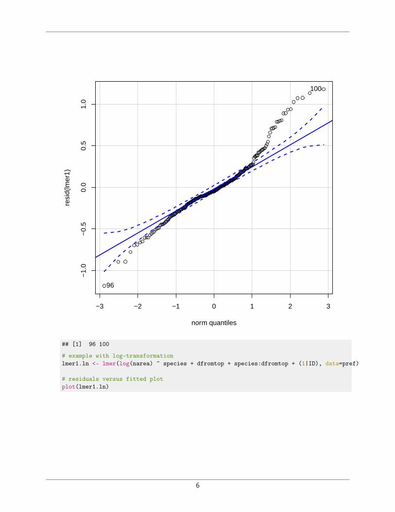
# visualise effect sizevisreg(mouse_m5, xvar='wheel')
## Conditions used in construction of plot## bm: 14.6## temp31: -11## id: 99## run: 2
9
0.0
0.1
0.2
0.3
0.4
wheel
f(w
heel
)
No Yes
2. ⧫ Inspect diagnostics for the best of the mouse models (use AIC on all models to choose the bestone), including QQ plot, and residuals versus fitted. Does a logarithmic transformation (eitherpredictor or response) improve the diagnostics?mouse_m5 <- lmer(rmr ~ bm*temp31 + wheel + (temp31|id/run), data=mouse)
plot(mouse_m5)
10

fitted(.)
resi
d(.,
type
= "
pear
son"
)
−0.2
−0.1
0.0
0.1
0.2
0.1 0.2 0.3
library(car)qqPlot(residuals(mouse_m5))
11

−3 −2 −1 0 1 2 3
−0.
2−
0.1
0.0
0.1
0.2
norm quantiles
resi
dual
s(m
ouse
_m5)
438
321
## 438 321## 429 318
3. ⧫ The mouse dataframe also contains a variable indicating the day on which the measurementstook place. Each mouse was exposed to each temperature once on each of six sequential days.Include day of measurement as another random effect, check whether the model fit is improved,and evaluate the significance of each of the fixed effects.mouse_m5 <- lmer(rmr ~ bm*temp31 + wheel + (temp31|id/run), data=mouse)mouse_m6 <- lmer(rmr ~ bm*temp31 + wheel + (temp31|id/day/run), data=mouse)anova(mouse_m5, mouse_m6)
## Data: mouse## Models:## mouse_m5: rmr ~ bm * temp31 + wheel + (temp31 | id/run)## mouse_m6: rmr ~ bm * temp31 + wheel + (temp31 | id/day/run)## Df AIC BIC logLik deviance Chisq Chi Df Pr(>Chisq)## mouse_m5 12 -2024.8 -1968.1 1024.4 -2048.8
12

## mouse_m6 15 -2221.1 -2150.2 1125.5 -2251.1 202.27 3 < 2.2e-16 ***## ---## Signif. codes: 0 '***' 0.001 '**' 0.01 '*' 0.05 '.' 0.1 ' ' 1
mouse_m7 <- lmer(rmr ~ bm*temp31 + wheel + (temp31|id/day), data=mouse)anova(mouse_m6, mouse_m7)
## Data: mouse## Models:## mouse_m7: rmr ~ bm * temp31 + wheel + (temp31 | id/day)## mouse_m6: rmr ~ bm * temp31 + wheel + (temp31 | id/day/run)## Df AIC BIC logLik deviance Chisq Chi Df Pr(>Chisq)## mouse_m7 12 -2146.6 -2089.9 1085.3 -2170.6## mouse_m6 15 -2221.1 -2150.2 1125.5 -2251.1 80.51 3 < 2.2e-16 ***## ---## Signif. codes: 0 '***' 0.001 '**' 0.01 '*' 0.05 '.' 0.1 ' ' 1
# residuals versus fitted plotplot(mouse_m6)
13

fitted(.)
resi
d(.,
type
= "
pear
son"
)
−0.1
0.0
0.1
0.1 0.2 0.3 0.4
# qqplotqqPlot(resid(mouse_m6))
14

−3 −2 −1 0 1 2 3
−0.
10−
0.05
0.00
0.05
0.10
0.15
norm quantiles
resi
d(m
ouse
_m6)
290530
## 290 530## 287 512
# fixed effects testAnova(mouse_m6, test='F')
## Analysis of Deviance Table (Type II Wald F tests with Kenward-Roger df)#### Response: rmr## F Df Df.res Pr(>F)## bm 18.9720 1 31.873 0.0001286 ***## temp31 77.6848 1 17.495 7.562e-08 ***## wheel 118.9145 1 102.668 < 2.2e-16 ***## bm:temp31 2.6467 1 51.324 0.1098908## ---## Signif. codes: 0 '***' 0.001 '**' 0.01 '*' 0.05 '.' 0.1 ' ' 1
15

4. ⧫ Take a subset of the mouse data where temperature (temp) is 31. Run a mixed-effects model ofresting metabolic rate with only sex (Male or Female) as predictor. Choose appropriate randomeffects. Does rmr vary with sex of the mouse?mouse31 <- subset(mouse, temp==31)
m31_1 <- lmer(rmr ~ sex + (1|run/id), data=mouse31)Anova(m31_1)
## Analysis of Deviance Table (Type II Wald chisquare tests)#### Response: rmr## Chisq Df Pr(>Chisq)## sex 9.7379 1 0.001805 **## ---## Signif. codes: 0 '***' 0.001 '**' 0.01 '*' 0.05 '.' 0.1 ' ' 1
5. ⧫ Now add body mass (bm) to the model with sex, as a main effect and interaction. Is sex stillsignificant? Use visreg to understand how bodymass, sex, and restingmetabolic rate are related.If it helps, also test whether body mass varies with sex.m31_2 <- lmer(rmr ~ bm*sex + (1|run/id), data=mouse31)Anova(m31_2)
## Analysis of Deviance Table (Type II Wald chisquare tests)#### Response: rmr## Chisq Df Pr(>Chisq)## bm 10.4487 1 0.001227 **## sex 0.9337 1 0.333891## bm:sex 0.0791 1 0.778544## ---## Signif. codes: 0 '***' 0.001 '**' 0.01 '*' 0.05 '.' 0.1 ' ' 1
visreg(m31_2, "bm", by="sex", overlay=TRUE)
16

10 12 14 16 18 20
0.05
0.10
0.15
0.20
0.25
bm
f(bm
)Female Male
1.10.3 Litter decomposition data
1. ∎ Generate some diagnostic plots for the litter_m1model described in Section ??.# Read datalitter <- read.csv("masslost.csv")
# Make sure the intended random effects (plot and block) are factorslitter$plot <- as.factor(litter$plot)litter$block <- as.factor(litter$block)
# Represent date as number of days since the start of the experimentlibrary(lubridate)
##
17

## Attaching package: ’lubridate’
## The following object is masked from ’package:base’:#### date
litter$date <- as.Date(mdy(litter$date))litter$date2 <- litter$date - as.Date("2006-05-23")
# fit modellitter_m1 <- lmer(masslost ~ date2 + herbicide * profile + (1|block/plot),
data = litter)
# residuals versus fitted plotplot(litter_m1)
fitted(.)
resi
d(.,
type
= "
pear
son"
)
−0.6
−0.4
−0.2
0.0
0.2
0.4
−0.2 0.0 0.2 0.4 0.6
18
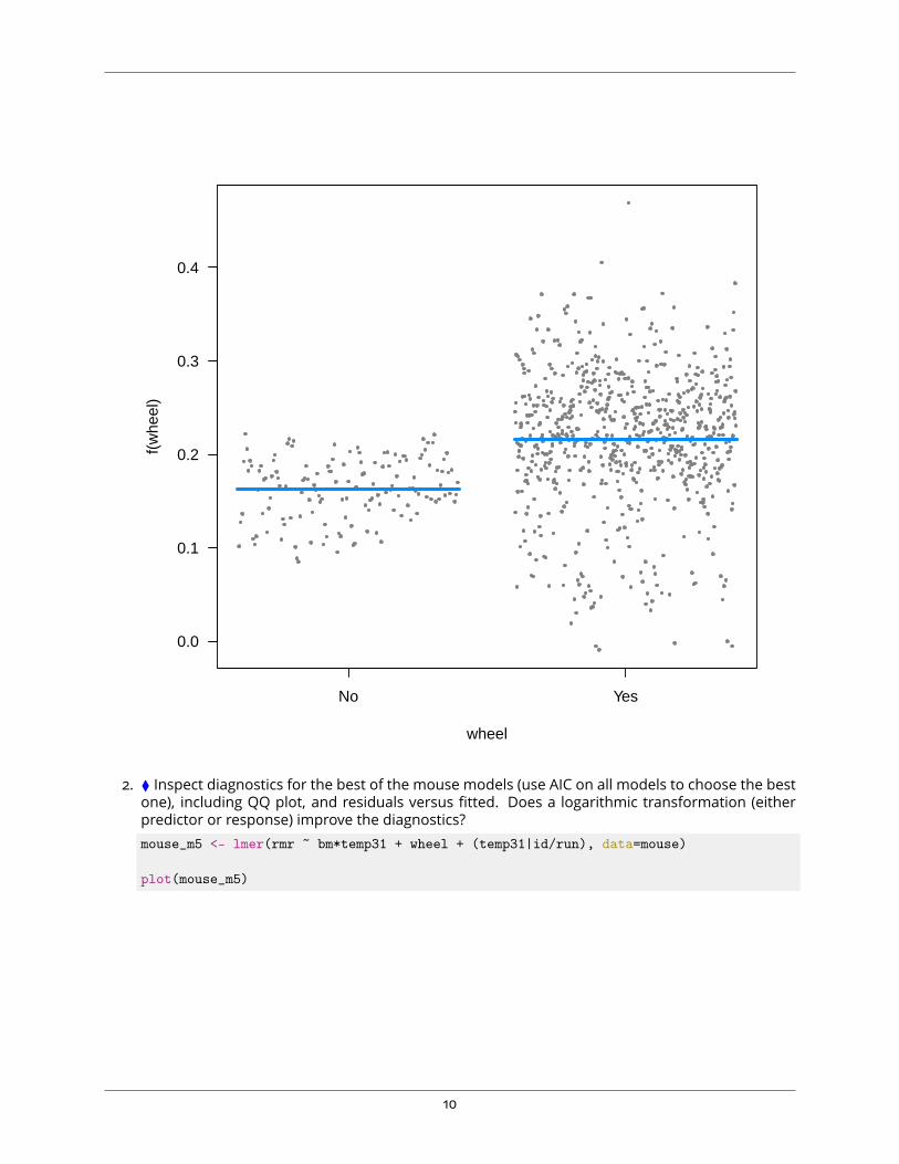
# qqplotqqPlot(resid(litter_m1))
−3 −2 −1 0 1 2 3
−0.
6−
0.4
−0.
20.
00.
20.
4
norm quantiles
resi
d(lit
ter_
m1)
171
165
## [1] 171 165
2. ⧫ The litter data contain a factor (variety) describing whether the litter is derived from a ge-netically modified (gm) or conventional (nongm) soy variety. Plot the data to observe the effect ofvariety. Use lmer to test the effect of variety, in addition to the other significant variables, onlitter decomposition.# Read data and get summarylitter <- read.csv('masslost.csv')
# Change random effects (plot and block) to factorslitter$plot <- as.factor(litter$plot)litter$block <- as.factor(litter$block)
19

# Represent date as number of days since the start of the experimentlibrary(lubridate)litter$date <- as.Date(mdy(litter$date))litter$date2 <- litter$date - as.Date('2006-05-23')
# look for treatment effectslibrary(lattice)bwplot(masslost ~ factor(date) | profile:herbicide:variety, data=litter, layout=c(2,4))
mas
slos
t
−0.5
0.0
0.5
1.0
2006−07−18 2006−08−29 2006−10−27
buried:conv:gm
2006−07−18 2006−08−29 2006−10−27
buried:conv:nongm
buried:gly:gm
−0.5
0.0
0.5
1.0buried:gly:nongm
−0.5
0.0
0.5
1.0surface:conv:gm surface:conv:nongm
surface:gly:gm
−0.5
0.0
0.5
1.0surface:gly:nongm
# there does not look to be much effect of 'variety' (look across two# columns - 'layout' argument controls this)
library(lme4)library(car)m1 <- lmer(masslost ~ date2 + herbicide * profile * variety + (1|block/plot), data = litter)
20

Anova(m1, test='F')
## Analysis of Deviance Table (Type II Wald F tests with Kenward-Roger df)#### Response: masslost## F Df Df.res Pr(>F)## date2 140.0675 1 231.436 < 2.2e-16 ***## herbicide 12.7977 1 3.005 0.0372580 *## profile 519.2389 1 231.498 < 2.2e-16 ***## variety 0.3392 1 231.424 0.5608858## herbicide:profile 11.7097 1 231.277 0.0007351 ***## herbicide:variety 0.4590 1 231.820 0.4987471## profile:variety 0.0758 1 231.795 0.7832914## herbicide:profile:variety 0.0051 1 231.304 0.9431549## ---## Signif. codes: 0 '***' 0.001 '**' 0.01 '*' 0.05 '.' 0.1 ' ' 1
# residuals versus fitted plotplot(m1)
21

fitted(.)
resi
d(.,
type
= "
pear
son"
)
−0.6
−0.4
−0.2
0.0
0.2
0.4
−0.2 0.0 0.2 0.4 0.6 0.8
# qqplotqqPlot(resid(m1))
22

−3 −2 −1 0 1 2 3
−0.
6−
0.4
−0.
20.
00.
20.
4
norm quantiles
resi
d(m
1)
171
165
## [1] 171 165
1.10.4 Repeated measures in leaf photosynthesis
For this exercise you will use the EucFACE leaf gas exchange dataset. First walk through Section ??before starting this exercise.1. Read the data, and add a new variable called WUE (water-use efficiency), calculated as Photo di-vided by Trmmol. This new variable represents the amount of CO2 taken up per unit water lost.
eucgas <- read.csv("eucface_gasexchange.csv")
eucgas$WUE <- with(eucgas, Photo / Trmmol)
2. ∎Make a barplot of WUE by Date and CO2 treatment, as shown in Section ??.
23

library(sciplot)bargraph.CI(Date, WUE, CO2, data=eucgas, legend=TRUE, ylab="WUE")
A B C D
WU
E
02
46
8 AmbEle
3. ∎ Fit a linear mixed-effects model with Treewithin Ring as the random effects structure, and Dateand CO2 as fixed effect. Fit a second model with additionally the interaction between Date andCO2; is the interaction significant (use both anova on the two models, and Anova on the modelwith the interaction).wue_m0 <- lmer(WUE ~ Date + CO2 + (1|Ring/Tree), data=eucgas)wue_m1 <- lmer(WUE ~ Date * CO2 + (1|Ring/Tree), data=eucgas)
# Likelihood ratio testanova(wue_m0, wue_m1)
## Data: eucgas## Models:## wue_m0: WUE ~ Date + CO2 + (1 | Ring/Tree)
24

## wue_m1: WUE ~ Date * CO2 + (1 | Ring/Tree)## Df AIC BIC logLik deviance Chisq Chi Df Pr(>Chisq)## wue_m0 8 288.64 307.99 -136.32 272.64## wue_m1 11 293.79 320.40 -135.89 271.79 0.8477 3 0.838
# Chi-square testAnova(wue_m1)
## Analysis of Deviance Table (Type II Wald chisquare tests)#### Response: WUE## Chisq Df Pr(>Chisq)## Date 23.0332 3 3.974e-05 ***## CO2 18.2081 1 1.980e-05 ***## Date:CO2 0.7605 3 0.8589## ---## Signif. codes: 0 '***' 0.001 '**' 0.01 '*' 0.05 '.' 0.1 ' ' 1
4. ⧫ Inspect the standard deviation of the random effects with VarCorr. Notice that the standarddeviation for the term Tree:Ring (trees within rings) is very small compared to the Ring randomeffect. A naive user might remove this random effect since it explains little variation. Why is thata bad idea?VarCorr(wue_m0)
## Groups Name Std.Dev.## Tree:Ring (Intercept) 0.00000## Ring (Intercept) 0.28164## Residual 1.26842
# The trees are the experimental units. If we remove it from the random effects structure, we assume# all measurements within rings are independent, and are thus committing pseudoreplication.
5. ▲ Look at the summary statement of the model for WUE that does not contain an interaction.Notice that Date D is significantly lower than the intercept (Date A). Refit the model without anintercept, and use glht to test whether Date D was lower than all of Date A, B and C. Hint: thisfollows closely the example shown at the end of Section ??.wue_m0_re <- lmer(WUE ~ Date + CO2 -1 + (1|Ring/Tree), data=eucgas)
library(multcomp)
## Loading required package: mvtnorm
## Loading required package: survival
## Loading required package: TH.data
## Loading required package: MASS
#### Attaching package: ’TH.data’
## The following object is masked from ’package:MASS’:#### geyser
#### Attaching package: ’multcomp’
## The following object is masked _by_ ’.GlobalEnv’:
25

#### litter
summary(glht(wue_m0_re, linfct=c("DateD - DateA = 0","DateD - DateB = 0","DateD - DateC = 0")))
#### Simultaneous Tests for General Linear Hypotheses#### Fit: lmer(formula = WUE ~ Date + CO2 - 1 + (1 | Ring/Tree), data = eucgas)#### Linear Hypotheses:## Estimate Std. Error z value Pr(>|z|)## DateD - DateA == 0 -0.9884 0.3955 -2.499 0.03435 *## DateD - DateB == 0 -1.3658 0.3955 -3.453 0.00164 **## DateD - DateC == 0 -1.7190 0.3703 -4.643 < 0.001 ***## ---## Signif. codes: 0 '***' 0.001 '**' 0.01 '*' 0.05 '.' 0.1 ' ' 1## (Adjusted p values reported -- single-step method)
6. ⧫ A colleague tells you that water-use efficiency may be lower on Date D because air temperaturewas higher, resulting in a lower air humidity. This is indicated by the variable VpdL in the dataset,which represents the ’vapour pressure deficit’ - higher values indicate drier air. Refit the modelfor WUE with the CO2*Date interaction, and now add VpdL as a fixed effect to the model (but nointeractions between VpdL and Date or CO2). Is VPD significant (use multiple methods to testthis)?wue_m2 <- lmer(WUE ~ VpdL + Date * CO2 + (1|Ring/Tree), data=eucgas)
Anova(wue_m2)
## Analysis of Deviance Table (Type II Wald chisquare tests)#### Response: WUE## Chisq Df Pr(>Chisq)## VpdL 36.5358 1 1.499e-09 ***## Date 36.2087 3 6.765e-08 ***## CO2 20.4753 1 6.040e-06 ***## Date:CO2 0.0718 3 0.995## ---## Signif. codes: 0 '***' 0.001 '**' 0.01 '*' 0.05 '.' 0.1 ' ' 1
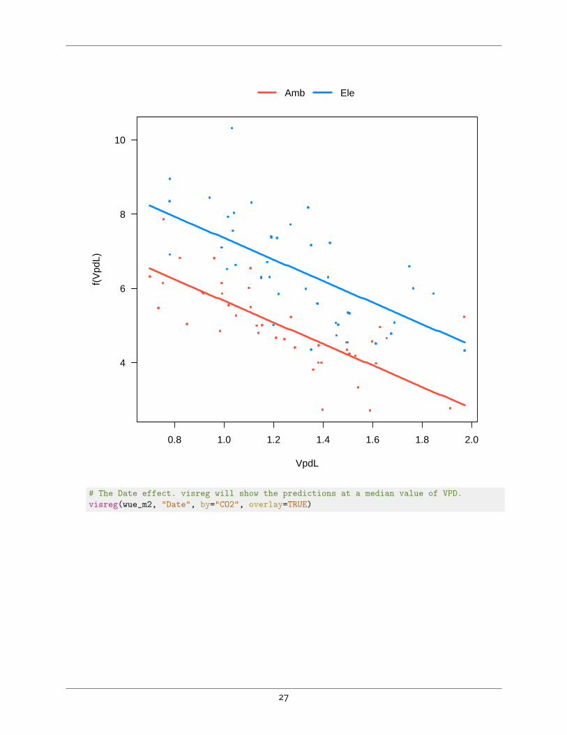
7. ▲ Use visreg to visualize a) the VpdL effect (make a visreg plot with VPD as the predictor, showingpredictions for both CO2 treatment), b) The Date effect. For this latter plot, use Date as the xvarargument to visreg, and CO2 as the by argument (with overlay=TRUE). For this last plot, visregwillshow the Date effect at a median value of VpdL, that is, the effect of VpdL has been removed first.Is Date D still different from the other Dates? Can you explain this in terms of the VpdL covariate?# VPD effect - visreg will take the first Date for the predictionsvisreg(wue_m2, "VpdL", by="CO2", overlay=TRUE)
26
0.8 1.0 1.2 1.4 1.6 1.8 2.0
4
6
8
10
VpdL
f(V
pdL)
Amb Ele
# The Date effect. visreg will show the predictions at a median value of VPD.visreg(wue_m2, "Date", by="CO2", overlay=TRUE)
27

4
5
6
7
8
9
10
Date
f(D
ate)
A B C D
Amb Ele
# The Dates are now very similar, and Date D is no longer lower. This means that VPD explained the lower# WUE on Date D, because in the above model its effect has been accounted for.# We can visually check this in the figure below. Note that Date D is lower, but also has higher VPD, and# all data for a CO2 treatment are mose or less on one line.with(eucgas, plot(VpdL, WUE, pch=c(19,3,6,1)[Date], col=c("blue","red")[CO2]))legend("topright", levels(eucgas$Date), pch=c(19,3,6,1))
28

0.8 1.0 1.2 1.4 1.6 1.8 2.0
45
67
89
10
VpdL
WU
E
ABCD
1.10.5 EucFACE ground cover data
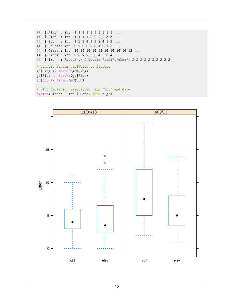
The file eucfaceGC.csv contains estimates of plant and litter cover within the rings of the EucFACEexperiment, evaluating forest ecosystem responses to elevated CO2, on two dates; the data descriptioncan be found in Section ?? (p. ??).1. ⧫ Convert the variables indicating the nested sampling design to factors, then use glmer in lme4to test for an interaction between Trt and Date on Litter cover. Litter cover represents counts(use the poisson family).
# read datagc <- read.csv('eucfaceGC.csv')str(gc)
## 'data.frame': 192 obs. of 8 variables:## $ Date : Factor w/ 2 levels "11/06/13","3/09/13": 1 1 1 1 1 1 1 1 1 1 ...
29
## $ Ring : int 1 1 1 1 1 1 1 1 1 1 ...## $ Plot : int 1 1 1 1 2 2 2 2 3 3 ...## $ Sub : int 1 2 3 4 1 2 3 4 1 2 ...## $ Forbes: int 0 2 0 0 2 5 4 0 1 3 ...## $ Grass : int 16 14 16 16 15 16 16 16 16 13 ...## $ Litter: int 5 6 2 2 3 3 4 3 0 4 ...## $ Trt : Factor w/ 2 levels "ctrl","elev": 2 2 2 2 2 2 2 2 2 2 ...
# convert random variables to factorsgc$Ring <- factor(gc$Ring)gc$Plot <- factor(gc$Plot)gc$Sub <- factor(gc$Sub)
# Plot variation associated with 'Trt' and datebwplot(Litter ~ Trt | Date, data = gc)
Litte
r
0
5
10
15
ctrl elev
11/06/13
ctrl elev
3/09/13
30

# Plot variation associated with plots and subplotsxyplot(Litter ~ Date | Ring, groups = Plot,
data = gc, pch = 16, jitter.x = TRUE)
Date
Litte
r
0
5
10
15
11/06/13 3/09/13
1 2
11/06/13 3/09/13
3
4
11/06/13 3/09/13
5
0
5
10
15
6
# fit model and test for effectsm2 <- glmer(Litter ~ Trt * Date + (1|Ring/Plot), data=gc, family=poisson)summary(m2)
## Generalized linear mixed model fit by maximum likelihood (Laplace## Approximation) [glmerMod]## Family: poisson ( log )## Formula: Litter ~ Trt * Date + (1 | Ring/Plot)## Data: gc#### AIC BIC logLik deviance df.resid## 923.2 942.8 -455.6 911.2 186##
31

## Scaled residuals:## Min 1Q Median 3Q Max## -2.22194 -0.66709 0.02852 0.54770 2.40787#### Random effects:## Groups Name Variance Std.Dev.## Plot:Ring (Intercept) 0.1023 0.3199## Ring (Intercept) 0.0867 0.2945## Number of obs: 192, groups: Plot:Ring, 24; Ring, 6#### Fixed effects:## Estimate Std. Error z value Pr(>|z|)## (Intercept) 1.45991 0.20529 7.111 1.15e-12 ***## Trtelev 0.01786 0.29009 0.062 0.950914## Date3/09/13 0.62952 0.08334 7.554 4.22e-14 ***## Trtelev:Date3/09/13 -0.42318 0.12015 -3.522 0.000428 ***## ---## Signif. codes: 0 '***' 0.001 '**' 0.01 '*' 0.05 '.' 0.1 ' ' 1#### Correlation of Fixed Effects:## (Intr) Trtelv D3/09/## Trtelev -0.707## Date3/09/13 -0.265 0.187## Tr:D3/09/13 0.184 -0.248 -0.694
library(car)Anova(m2)
## Analysis of Deviance Table (Type II Wald chisquare tests)#### Response: Litter## Chisq Df Pr(>Chisq)## Trt 0.7057 1 0.400889## Date 50.3421 1 1.291e-12 ***## Trt:Date 12.4057 1 0.000428 ***## ---## Signif. codes: 0 '***' 0.001 '**' 0.01 '*' 0.05 '.' 0.1 ' ' 1
2. Make model diagnostics plot for the model of Grasswith treatment and Date as fixed effects. Usethe DHARMa package as shown in Fig. ??. Now refit this model with the poisson family - which is awrong model specification because Grass count is clearly bounded by a maximum (16 quadrantsin each plot). Make the model diagnostic plot again, and note how it has changed.library(DHARMa)
# 'correct' modelm1 <- glmer(cbind(Grass, 16-Grass) ~ Trt * Date + (1|Ring/Plot),
data=gc, family=binomial)
# Does not look great, though.plotSimulatedResiduals(simulateResiduals(m1))
32

0.0 0.2 0.4 0.6 0.8 1.0
0.0
0.2
0.4
0.6
0.8
1.0
QQ plot residuals
Expected
Obs
erve
d
KS test: p= 0.04083Deviation significant
Residual vs. predicted lines should match
Predicted value
Sta
ndar
dize
d re
sidu
al
0.80 0.90 1.00
0.00
0.25
0.50
0.75
1.00
DHARMa scaled residual plots
# incorrect modelm1_bad <- glmer(Grass ~ Trt * Date + (1|Ring/Plot),
data=gc, family=poisson)
# Very bad!plotSimulatedResiduals(simulateResiduals(m1_bad))
33

0.0 0.2 0.4 0.6 0.8 1.0
0.0
0.2
0.4
0.6
0.8
QQ plot residuals
Expected
Obs
erve
d
KS test: p= 0Deviation significant
Residual vs. predicted lines should match
Predicted value
Sta
ndar
dize
d re
sidu
al
0.75 0.85 0.95
0.00
0.25
0.50
0.75
1.00
DHARMa scaled residual plots
1.10.6 Logistic regression
For this exercise, we will use the seed germination data (fire experiment). First walk through Section ??.1. For the seedfire dataset, the examples in the text use temp as a factor variable. Attempt to insteaduse it as an (untransformed) continuous variable in the model. Compare the model with temp asa factor and temp as a factor, in terms of AIC. Now plot diagnostic plots for both models (seeSection ??). Ignore the warning.
seedfire <- read.csv("germination_fire.csv")
# Make sure temperature treatment is a factorseedfire$temp <- as.factor(seedfire$temp)
# temp as factor
34

firefit1 <- glmer(cbind(germ, n-germ) ~ species + temp +(1|site), data=seedfire, family=binomial)
# temp as numeric predictorseedfire$temp_c <- as.numeric(as.character(seedfire$temp))
firefitc1 <- glmer(cbind(germ, n-germ) ~ species + temp_c +(1|site), data=seedfire, family=binomial)
library(DHARMa)plotSimulatedResiduals(simulateResiduals(firefit1))
0.0 0.2 0.4 0.6 0.8 1.0
0.0
0.2
0.4
0.6
0.8
1.0
QQ plot residuals
Expected
Obs
erve
d
KS test: p= 0Deviation significant
Residual vs. predicted lines should match
Predicted value
Sta
ndar
dize
d re
sidu
al
0.2 0.4 0.6 0.8 1.0
0.00
0.25
0.50
0.75
1.00
DHARMa scaled residual plots
plotSimulatedResiduals(simulateResiduals(firefitc1))
35

0.0 0.2 0.4 0.6 0.8 1.0
0.0
0.2
0.4
0.6
0.8
1.0
QQ plot residuals
Expected
Obs
erve
d
KS test: p= 0Deviation significant
Residual vs. predicted lines should match
Predicted value
Sta
ndar
dize
d re
sidu
al
0.4 0.6 0.8 1.0
0.00
0.25
0.50
0.75
1.00
DHARMa scaled residual plots
2. Try to understand why temp as a continuous variable does so badly, using visreg (set temp as thexvar, and also use scale="response"). Compare the fitted response to the data (i.e., also make aplot of germination success versus temperature, and compare to the visreg plot).visreg(firefitc1, "temp_c", scale="response")
36

10 15 20 25 30 35
0.3
0.4
0.5
0.6
0.7
0.8
0.9
temp_c
cbin
d(ge
rm, n
− g
erm
)
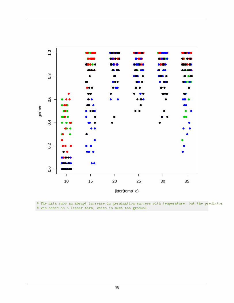
# Compare to:palette("default")with(seedfire, plot(jitter(temp_c), germ/n, col=species, pch=19))
37
10 15 20 25 30 35
0.0
0.2
0.4
0.6
0.8
1.0
jitter(temp_c)
germ
/n
# The data show an abrupt increase in germination success with temperature, but the predictor# was added as a linear term, which is much too gradual.
38