Embed Size (px)
Citation preview
;^ll ri^-!<'!
•\ —-. •'.iUV•r> ^ •
'v\ •* ^ i^j
ERIC CHANG'S COPY
VISCOUS FINGERING IN
HETEROGENEOUS POROUS MEDIA
Udo Gaetan Araktingi
June 1988
Miscible Flooding Research
DEBSffiEMENrOFBETHQLEnM:ENGINEEHIFS

VISCOUS FINGERIfIG IN
HETEROGENEOUS POROUS MEDIA
A DISSERTATION
SUBMITIED TO THE DEPARTMENT OF PETROLEUM ENGINEERING
AND THE COMMnTEE ON GRADUATE STUDIES
OF STANFORD UNIVERSITY
IN PARTIAL FULFILLMENT OF THE REQUIREMENTS
FOR THE DEGREE OF
DOCTOR OF PHILOSOPHY
By
Udo Gaetan Aiaktingi
June 1988

ACKNOWLEDGEMENTS
I wish to express my gratitude and s^redation to
Professor Franklin M. Orr, Jr. - wbo l^ped me formulate and solve this problem andshared witfi me his experience, knowledge and insight;
Professors Andre Joumel, William E. Brigham and Khalid Aziz - for tl^ir he^Mcommits and suggestions;
• Professor Henry J. Ramey - for accepting me into the doctoral program and believingthat I could handle the challenge;
• The Department of Energy - which made my graduate study at Stanford possiblethrough tfie grant of a research assistantship.
u

ABSTRACT
Performance of miscible flood enhanced oil recovery processes is often influenced by
tiie effects of viscous instability which cause fingers of the low viscosity injected fluid to
invade the fluid in place, but little is known about the effects of the reservoir hetero
geneities on the growth of fingers. In this research I describe a new approach to modeling
of viscous fingering based on random-walk techniques, and use the new model to examine
tiie growth of viscous fingers in heterogeneous porous media. The fluid is represented as a
discrete set of particles, each particle assuming a unit volume. The movement of the parti
cles through the porous medium is the result of two types of motion. One motion is along
the flow streamlines. The second is random motion, governed by scaled probability curves
related to flow length and the longitudinal and transverse dispersion coefficients.
The resulting algorithm was validated against one-dimensional analytic^ solutions for
miscible displacements with unit viscosity ratio to show that appropriate longitudinal and
transverse Peclet numbers are recovered and that effects of numerical dispersion are small.
Next, model calculations were compared with experimental results for miscible displace
ments in horizontal beadpacks (Blackwell et a/., 1959) and in vertical sections (Pozzi and
Blackwell, 1963) with mobility ratios ranging between 1.85 and 375 and viscous to gravity
numbers ratios from 89 to 200,000. Excellent agreement was obtained between the simula
tions and experiments without any adjustment of parameters to achieve a match. The
effects of mobility ratio and injection rate on unstable displacements in homogeneous sands
were examined, and the observation made by Koval (1963), that each concentration contour
moves at an approximately constant characteristic velocity, was confirmed.
Stochastically generated permeability fields were used to study the interaction between
viscous fingering and heterogeneities in the porous media. The heterogeneity index(GeIhar,
1986, Mishra, 1987), defined as tiie product of a dimensionless correlation length, Xd, and
the variance of the log-normal permeability distribution, was used to characterize each
penneability realization. The physical processes involved in these imstable displacements
m

were examined by analysis of velocities of averaged concentrations and growth of the mix
ing zone. For mildly heterogeneous penneability fields (low Xd), concentration contour
velocities remained approximately constant and the mixing zone grew lineaily with time.
However, for displacements in more heterogeneous penneability fields (o4 > 0.5), the
penneability distribution controlled finger growth. For heterogeneiQr indices smaller than
about 0.3, viscous forces dominated finger growth, and fingering patterns were similar to
those observed in homogeneous permeability fields. In such cases, viscous crossfiow
caused fast moving fingers to split at their tips and to coalesce with neighboring fingers at
their tails. Displacement performance was quite sensitive to the level of transverse disper
sive mbdng when the heterogeneity index was low. When the heterogeneity index was
larger than about 0.5, however, the pattern of fingers conformed to preferential flow paths
in the penneability distribution, and transverse mixing had minimal impact on displacement
perfonnance. Neither mechanism clearly dominated fingering behavior for the region of
heterogeneity indices between 0.3 and 0.5.
IV

TABLE OF CONTENTS
Eagg
ACKNOWLEDGEMENT iiABSTRACT iiiLIST OF HGURES viiLIST OF TABLES xv
1. INTRODUCnON 11.1 Literature Survey 2
2. MODEL FORMULATION 6
2.1 Model Description. 62.2 Model Algorithm 172.3 Inclusion of Gravity 182.4 Probabilistic Approach 23
3. VALIDATION 263.1 Random Walk Model 26
3.1.1 Analytical Solutions 263.1.2 Recovery of Input Dispersion Values 373.1.3 Comparison with Experimental Results .413.1.4 Model Perfonnance Characteristics 44
3.2 Random Walk Model with Gravity 473.3 Probabilistic Model 543.4 Summary 60
4. DISPLACEMENTS IN HOMOGENEOUS POROUS MEDIA 634.1 Late Time Behavior 634.2 Velocity Behavior 804.3 Mixing Zone 864.4 Linear Stability Theory .-88
5. DISPLACEMENTS IN HETEROGENEOUS POROUS MEDL\ 925.1 Representation of Heterogeneous Media 925.2 Heterogeneity Index Concept 945.3 Qualitative Validation 945.4 Flow Behavior. 99
5.5 Velocity Behavior 1415.6 Fmger Width 1415.7 Comparison of Simulation Results with Koval*s Theory 148
6. DISCUSSION 1596.1 Model Advantages u. 1606.2 Model Disadvantages.......i.... : 1616.3 Viscous Fingering and Permeability Heterogeneities 1616.4 Scaling 166
6.4.1 Field Scale Simulation 1686.4.2 Validity of C-D Equation for Heterogeneous Media 169
7. CONCLUSIONS RECOMMENDATIONS 1737.1 Conclusions 1737.2 Recommendations 174
NOMENCLATURE 176REFERENCES 178APPENDICES 182A. Finite Differencing of Diffusivity Equation 182B. Finite Differencing of Diffusivity Equation including Gravity 184C. Spectral Analysis 187D. Finger Width Measurement 189

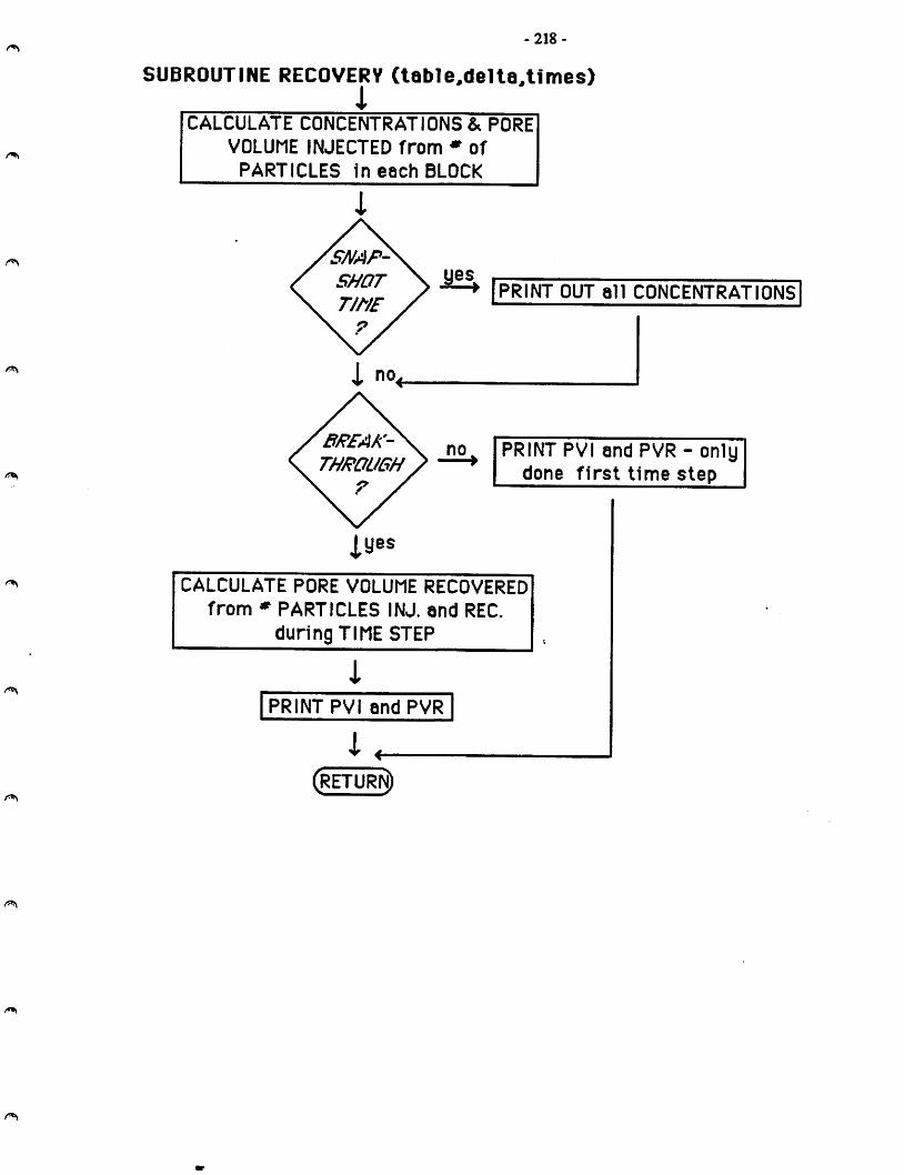
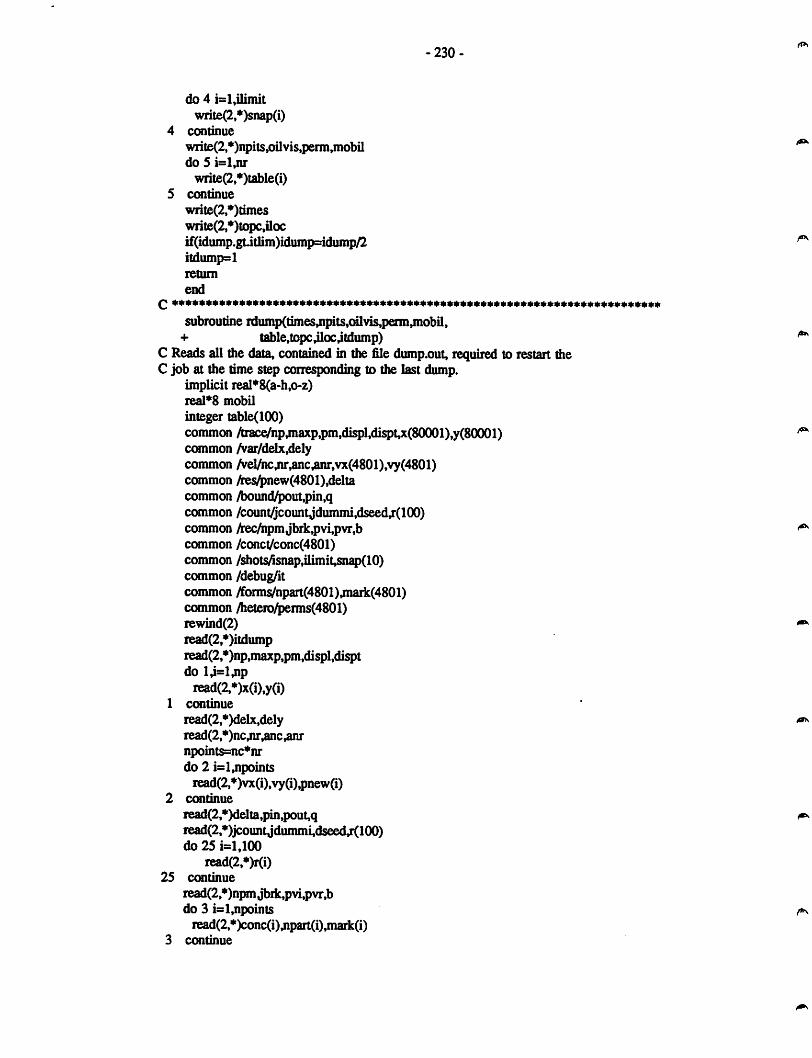
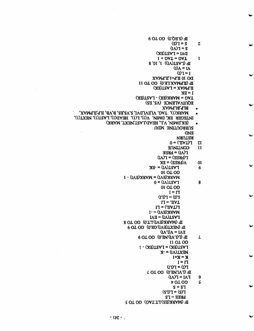
E. Peimeability Fields 191F. Derivation of Dispersion Coefficients from Experimental Data 212G. Flowcharts of Main Program and Subroutines 214H. Computer Code 223 ^
VI

LIST OF FIGURES
Page
2.1 Basic concepts for the random-walk model 7
2.2 Solution of Convection-Dispersion equation (Bear, 1972) 10
2.3A Longitudinal dispersion step in model when displacementis aligned with x-y coordinate system 12
2.3B Transverse dispersion step in model when displacementis aligned with x-y coordinate system 13
2.4A Longitudinal dispersion step in model for general case 14
2.4B Transverse dispersion step in model for general case 15
2.5 Vector algebra for dispersion step 16
2.6A First step in calculating x and y velocity vectors for particle 19
2.6B Second step in calculating x and y velocity vectors for particle 20
2.6C Final step in calculating x and y velocity vectors for partide 21
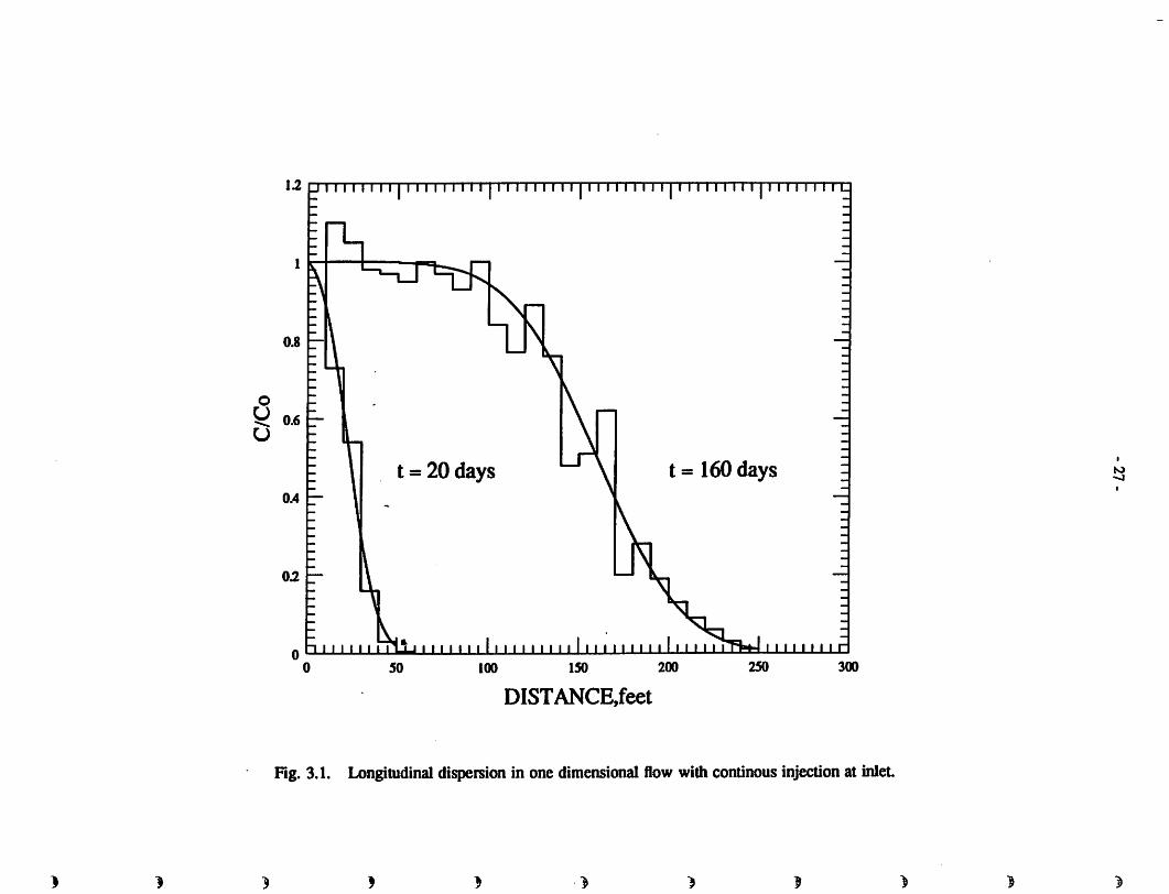
3.1 Longitudinal dispersion in one dimensional flow withcontinous injection at inlet 27
3.2A Longitudinal dispersion in uniform one-dimensionalflow with a slug of tracer injected at inlet (100 particles) 29
3.2B Longitudinal dispersion in uniform one-dimensionalflow with a slug of tracer injected at inlet (200 particles) 30
3.2C Longimdinal dispersion in unifonn one-dimensionalflow with a slug of tracer injected at inlet (300 panicles) 31
3.3A Dispersion of a slug injected in ^unifonn one-dimensional flow in the x direction 32
3.3B Longitudinal distribution on both sides of themean flow after 20 days 33
3.3C Transverse distribution on both sides of themean flow after 20 days 34
3.3D Longitudinal distribution on both sides of themean flow after 70 days 35
3.3E Transverse distribution on both sides of themean flow after 70 days 36
y PW
3.4A Plot of eif^ (1 - 2C ) versus —Vm
vii

•{pZThe dope of the resulting line is equal to 38
3.4B Longitudinal Pe number as a function of grid size' and seed number.N is the number of grid blocks in the longitudinal direction 39
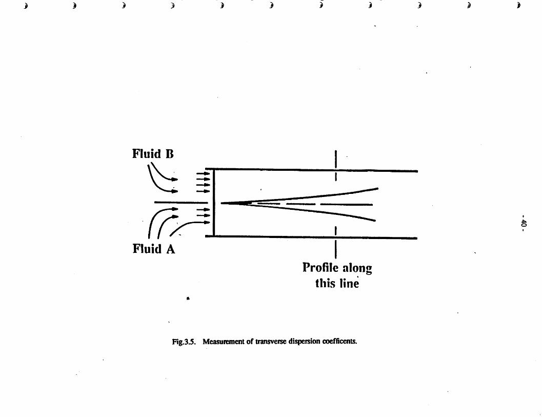
3.5 Measurement of transverse dispersion coefficents 40
3.6 Transverse Pe number as a function of grid size and seed number. N is thenumber of grids in the transverse direction 42
3.7 Comparison of random-walk model results with Blackwell's experimentalresults 43
3.8 Dependence of recovery for M=375 on grid size 45
3.9 Dependence of recoveries on choice of seed number. 46
3.10A Dependence of recovery on number of particles injected per grid block.Simulation result is shown as solid line 48
3.10B Effect of grid orientation on recovery for M=15 displacement .49
3.11 Comparison of random-walk model results (with gravity included) withBlackwell's experimental results. Simulation predictions are ^own assolid lines 53
3.12 Illustration of the different flow regimes (after Stalkup) 55
3.13 Cross-sectional displacements for the conditions indicated showing 0.05concentration contour line at different times 56
3.14 Calculated concentration contours (a) and streamlines (b) for viscosityratio of 375 at 0.15 pore volumes injected 58
3.15 Effects of variations of grid block size as a fimction of time step 59
3.16 LongimdinalPeclet number vs. time step as a fimction of gridblock size 59
3.17 Effects of variations of grid block size when transverse dispersion isincluded 61
4.1A Displacementfor M=10, V=40 fVD, showing 0.2 concentration contour liiKin homogeneous pemieability field. (A) corresponds to PVI=0.1, (B) toPVI=0.2, (C) to PVI=0.3 65
4.1B Displacement for M=10, V=40 ft/D, showing0.2 concentration contour line inhomogeneous pemieability field. (D) corresponds to PVI=0.4, (E) toPVI=0.5, (F) to PVI=0.6 66
4.2 Displacement for M=50, V=40 ft/D, showing 0.2 concentration contour line inhomogeneous permeability field. (A) corresponds to PVI=0.1, (B) toPVI=0.2. (C) to PVI=0.3 67
Vlll

4.3A Displacement for M=1(X), V=40 ft/D, showing 0.2 concentration contour linein homogeneous permeability field. (A) corresponds to PVI=0.05 (B) toPVI=0.1. (C) to PVI=0.15 68
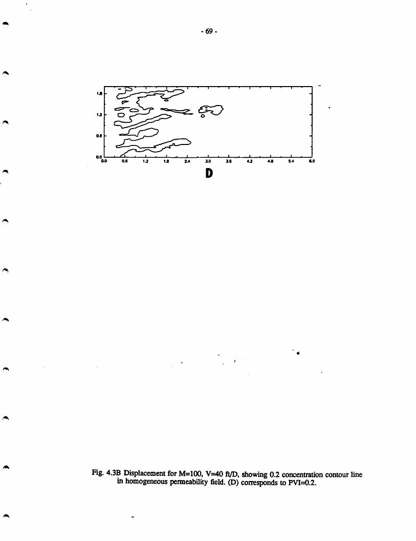
4.3B Displacement for M=100, V=40 ft/D, showing 0.2 concentration contour linein homogeneous permeability field. (D) corresponds to PVI=0.2 69
4.4A Displacement for M=10, V=10 fVD, showing 0.2 concentration contour line inhomogeneous permeability field. (A) conesponds to PVI=0.1, (B) toPVI=0.2. (C) to PVI=0.3 70
4.4B Displacement for Ms10, V=10 ft/D, showing 0.2 concentration contour line inhomogeneous permeability field. (A) corresponds to PVI=0.4, (B) toPVI=0.5, (C) to PVI=0.6 71
4.5A Displacement for M=50, V=10 ft/D, showing 0.2 concentration contour line inhomogeneous permeability field. (A) conesponds to Pyi=0.1, (B) toPVI=0.2, (C) to PVI=0.3 72
4.5B Displacement for M=50, V=10 ft/D, showing 0.2 concentration contour line inhomogeneous permeability field. (A) conesponds to PVI=0.4, (B) toPVI=0.5. (C) to PVI=0.6 73
4.6 Displacement for M=100, V=10 ft/D, showing 0.2 concentration contour linein homogeneous pemieability field. (A) corresponds to PVI=0.,05 (B) toPVI=0.1, (C) to PVI=0.15 74
4.7A Displacement for M=10, V=0.5 fl/D, showing 0.2 concentration contour linein homogeneous pemieability field. (A) corresponds to PVI=0.1, (B) toPVI=0.2. (C) to PVI=0.3 75
4.7B Displacement for M=10, V=0.5 ft/D, showing 0.2 concentration contour linein homogeneous permeability field. (D) corresponds to PVI=0.4, (E) toPVI=0.5 76
4.8A Displacement for M=50, V=0.5 ft/D, showing 0.2 concentration contour linein homogeneous permeability field. (A) conesponds to PVI=0.1 (B) toPVI=0.2, (C) to PVI=0.3 77
4.8B Displacement for M=550, V=0.5 iiJD, showing0.2 concentration contour linein homogeneous permeability field. (D) coriesponds to PVI=0.4 78
4.9 Displacement for M=100, V=0.5 ft/D, showing 0.2 concentration contour linein homogeneous permeability field. (A) corresponds to PVI=0.05 (B) toPVI=0.1. (C) to PVI=0.15 79
4.1OA Plot of averaged concentration position versus time. All existinglocations are shown 82
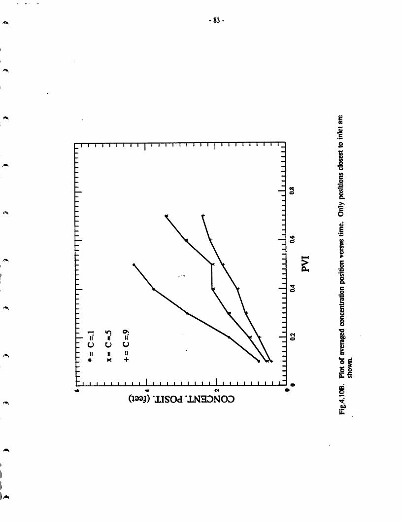
4.1OB Plot of averaged concentration positionversus time. Only positionsclosest to inlet are shown 83
4.IOC Plot of averaged concentration position versus time. Only positionsftmhest to inlet are shown 84
IX

4.10D Plot of averaged concentration position versus time. Arithmeticaverages of the positions are shown 85
4.11 Plot of mixing zone length versus time showingfluee different regions 87
5.1 Approximate representation of the pemieability field used in dieflow visualization experiments done by >^^thjack. 95
5.2 Displacement for M=l, V=40 fl/D, showing 0.2 concentration contour line inpenneability field shown in Rg. 5.1.
(A) corresponds to PVI=0.05, B) to PVI=0.1, (C) to PVI=0.2 96
5.3A Displacement for M==69, V=40 fl/D, showing 0.2 concentration contour line inpemieability field shown in Fig. 5.1.
(A) coire^nds to PVI=0.05 0 to PVI=0.1, (C) to PVI=0.2 97
5.3B Displacement for M=69, V=40 ft/D, showing 0.2 concentration contour linein permeability field shown in Hg. 5.1.
(A) corresponds to PVI=0.05 (B) to PVI=0.1, (Q to PVI=0.2 98
5.4A Displacement for M=20, V=40 ft/D, showing 0.2 concentration contour linepemieability field #1 shown in Appendix E.
(A) corresponds to PVI=0.1, (B) to PVI=0.2, (Q to PVI=0.3 100
5.4B Displacementfor M=20, V=40 ft/D, showing 0.2 concentration contour linein permeability field #1 shown in Appendix E.(D) corresponds to PVI=0.4, (E) to PVI=0.5, (F) to PVI=0.6 101
5.5A Displacement for M=20, Vs=40 fil/D, showing 0.2 concentration contour line inpemieability field #2 shown in Appendix E.(A) corresponds to PVI=0.05, (B) to PVI=0.1, (Q to PVI=0.2 102
5.5B Displacement for M=20, V=40 ft/D, showing 0.2 concentration contourline inpemieability field #2 shown in Appendix E.(D) corresponds to PVI=0.3, (E) to PVI=0.4, (F) to PVI=0.6 103
5.6A Displacement for M=20, V=40 ft/D, showing 6.2 concentration contour line inpemieability field #3 show^ in Appendix E.(A) corresponds to pyi=0.05,' TO to PVI=Q.l, (Q to PVI=0.2 104
5.6B Displacement for M=20, V=40 ft/D, showing 0.2 concentration contour line inpemieability field #3 shown in Appendix E.(D) corresponds to PVI=0.3, (E) to PVI=0.4, (F) to PVI=0.5 105
5.7A Displacement for M=20, V=40 ft/D, lowing 0.2 concentration contourline inpemieability field #4 shown in Appendix E.(A) coiresponds to PVI=0.05, (B) to PVI=0.1, (O to PVI=0.15 106
5.7B Displacement for M=20, V=40 ft/D, showing 0.2 concentration contourline inpenneability field #4 shown in AppendixE.(D) corresponds to PVI=0.2, (E) to PVI=0.25 107
5.8A Displacement for M=20, V=40 ft/D, showing 0.2 concentration contour line in

penneability field #5 shown in Appendix E.(A) corresponds to PVI=0.05, (B) to PVI=0.1, (O to PVI=0.15 108
5.8B Displacement for M=20, V=40 ft/D, showing 0.2 concentration contour line inpenneability field #5 shown in Appendix E.(D) corresponds to PVI=0.2, (E) to PVI=0.25, (F) to PVI=0.3 109
5.8C Displacement for M=20, V=40ft/D, showing 0.2 concentration contour linein penneability field #20 shown in Appendix E. (A) corresponds toPVI=0.05, (B) to PVI=0.1, (C) to PVI=0.2 110
5.8D Displacement for M=20, V=40ft/D, showing 0.2 concentration contour linein permeability field #20 shown in Appendix E. (D) corresponds toPVI=0.3. (E) to PVI=0.4;(F) to PVI=0.5 Ill
5.8E Displacement for M=20, V=40ft/D, showing 0.2 concentration contour linein permeability field #18 shown in Appendix E. (A) corresponds toPVI=0.05, (B) to PVI=0.1. (C) to PVI=0.2 112
5.8F Displacement for M=20, V=40ft/D, showing 0.2 concentration contour linein permeability field #18 shown in Appendix E. (D) corresponds toPVI=0.3, (E) to PVI=0.4, (F) to PVI=0.5 113
5.8G Displacement for M=20, V=40ft/D, showing 0.2 concentration contour linein permeability field #19 shown in Appendix E. (A) corresponds toPVI=0.05, (B) to PVI=0.1, (O to PVI=0.2 114
5.8H Displacement for M=20, V=40fiyD, showing 0.2 concentration contour linein permeability field #19 shown in Appendix E. (D) corresponds toPVI=0.3, (E) to PVI=0.4, (F) to PVI=:0.5 115
5.9A Displacement for M=:20, V=40 ft/D, showing 0.2 concentration contour line inpenneability field #6 shown in Appendix E.(A) conesponds to PVI=0.05, (B) to PVI=0.1, (Q to PVI=0.15 116
5.9B Displacement for M=20, V=40 ft/D, showing 0.2 concentration contour line inpenneability field #6 shown in Appendix E.(D) conesponds to PVI=0.2. (E) to PVI=0.25. (F) to PVI=0.3 117
' * -
S.lOA Displacement for M=20, V=40 ft/D, showing 0.2 concentration contour linein penneability field #7 shown in Appendix E.(A) conesponds to PVI=0.05, (B) to PVI=0.1, (C) to PVI=0.15 118
5.10B Displacement for M=20, V=40 ft/D, showing 0.2 concentration contoiu* linein penneability field #7 shown in Appendix E.(D) corresponds to PVI=0.2, (E) to PVI=0.25, (F) to PVI=0.3 119
5.11A Displacement for M=20, V=40 ft/D, showing 0.2 concentration contour linein penneability field #8 shown in Appendix E.(A) conesponds to PVI=0.025, (B) to PVI=0.05. (Q to PVI=0.1 120
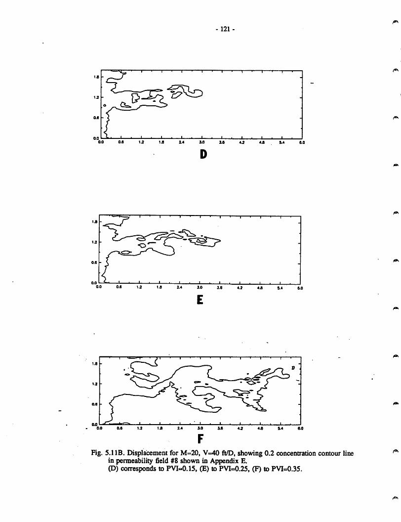
5.1 IB Displacement for M=20, V=40 ft/D, showing 0.2 concentration contour lineinpenneability field #8 ^owninAppendix E.G>) conesponds to PVI=0.95, (E) to PVI=0.15, (F) to PVI=0.35 121
XI
5.12A Displacement for M=20, V=40 fl/D, showing 0.2 concentration contour linein permeability field #9 shown in Appendix E.(A) corresponds to PVI=0.05, (B) to PVI=0.1, (C) to PVI=0.15 122
5.12B Displacementfor M=20, V=40 fl/D, showing 0.2 concentration contour linein permeability field #9 shown in Appendix E.(D) corresponds to PVI=0.175, (E) to PVI=0.2, (F) to PVI=0.25 123
5.13A Displacementfor M=20, V=40 fl/D, showing 02 concentration contour linein penneability field #10 shown in Appendix E.(A) corresponds to PVI=0.05, (B) to PVI=0.1, (Q to PVI=0.15 124
S.13B Displacementfor M=20, Vs40 fl/D, showing 0.2 concratration contour linein penneability field #10 shown in Appendix E.
(D) corresponds to PVI=0.2, (E) to PVI=0.25 125
5.14A Displacement for M=20, V=40 fl/D, showing 0.2 concentration contour linein penneability field #11 shown in Appendix E.(A) corresponds to PVI=0.05. (B) to PVI=0.1. (Q to PVI=0.15 126
5.14B Displacementfor M=20, V=40 fl/D, showing 0.2 concoitration contour linein penneability field #11 shown in Appendix E.(D) corresponds to PVI=0.175, (E) to PVI=0.2, (F) to PVI=0.25 127
5.15A Displacement for M=20, V=40 fl/D, showing0.2 concentration contour linein penneability field #12 shown in AppendixE.(A) corresponds to PVI=0.05, (B) to PVI=0.1, (C) to PVI=0.15 128
5.15B Displacement for M=20, V=40 fl/D, showing 0.2 concentration contourlinein penneability field #12 shown in Appendix E.(D) corresponds to PVI=0.175, (E) to PVI=0.2, (F) to PVI=0.25 129
5.16A Displacement for M=20, V=40 fl/D, showing 0.2 concentration contour linein penneability field #13 shown in Appendix E.(A) corresponds to PVI=0.05, (B) to PVI=0.1, (Q to PVI=0.95 130
5.16B Displacement for M=20, V=40 fl/D, showing 0.2 concentration contour linein penneability field #13 shown in Appendix E.(D) corresponds to PVI=ai5, (E) to PVI=0.175, (F) to PVI=0.2 131
5.17A Displacement for M=20, V=40 fl/D, showing 0.2 concentration contour linein penneability field #14 shown in Appendix E.(A) corresponds to PVI=0.05, (B) to PVI=0.1, (Q to PVI=0.125 132
5.17B Displacement for M=20, V=40 fl/D, showing 0.2 concentration contour linein permeability field #14 shown in Appendix E.(D) corresponds to PVI=0.15, (E) to PVI=0.175. (F) to PVI=0.2 133
5.18A Displacement for M=20, V=40 fl/D, showing 0.2 concentration contour linein permeability field #15 shown in Appendix E.(A) corresponds to PVI=0.025, (B) to PVI=0.05, (Q to PVI=0.075 134
5.18B Displacement for M=20, V=40 fl/D, showing 0.2 concentration contour linein penneability field #15 shown in Appendix E.
Xll

(D) corresponds to PVI=0.1, (E) to PVI=0.125 135
5.19A Displacement for M=20, V=40 ft/D, showing 0.2 concentration contour linein peraieability field #16 shown in Appendix E.(A) corresponds to PVI=0.05, (B) to PVI=0.1. (C) to PVI=0.125 136
5.19B Displacement for M=20, V=40 ft/D, showing 0.2 concentration contour linein permeability field #16 shown in Appendix E.(D) corresponds to PVI=0.15, (E) to PVI=0.2, (F) to PVI=0.25 137
5.20A Displacement for M=20, V=40 fl/D, showing 0.2 concentration contour linein permeability field #17 shown in Appendix E.(A) corresponds to PVI=0.025, (B) to PVI=0.05, (C) to PVI=0.075 138
5.20B Displacement for M=20, V=40 ft/D, showing 0.2 concentration contour linein permeability field #17 shown in Appendix E.(D) corresponds to PVI=0.1, (E) to PVI=0.125 139
5.21A Plot of averaged concentration position versus time. Allexisting locations are shown 142
5.2IB Plot of averaged concentration position versus time. Onlypositions closest to inlet are shown 143
5.2 IC Plot of averaged concentration position versus time. Onlypositions fiirthest to inlet are shown 144
5.21D Plot of averaged concentration position versus time. Arithmeticaverages of the positions are shown 145
5.22 Plot of mixing zone length versus time showingthree different regions 146
5.23A Finger width growth. Group1. Symbols correspond to the differentheterogeneity index 149
5.23B Finger width growth. Group2. Symbols correqwnd to the differentheterogeneity index 150
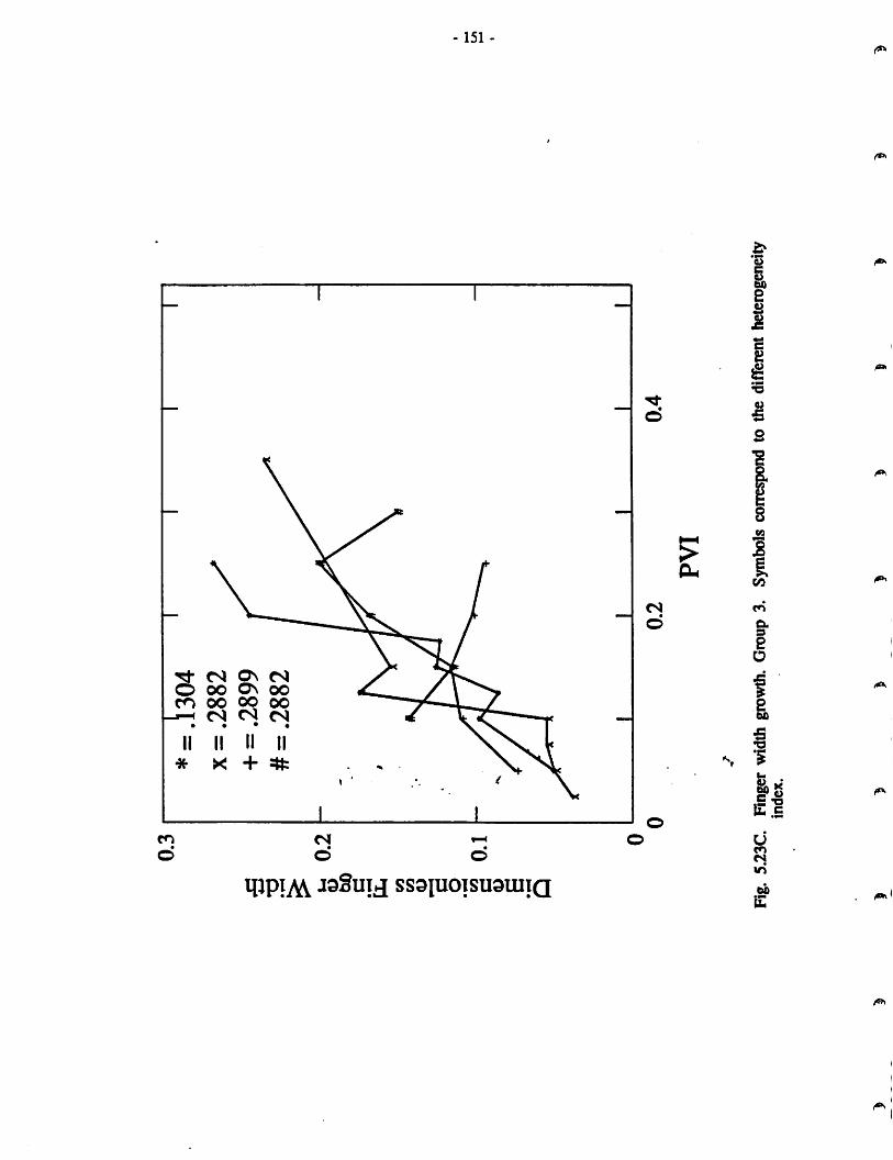
5.23C Fingerwidth growth. Group3. Symbols comespond to tiie differentheterogeneity index 151
5.23D Finger width growth. Group4. Symbols correspond to the differentheterogeneity index 152
5.23E Finger width growth. Group5. Symbols correspond to the differentheterogeneity index 153
5.23F Finger width growth. Group6. Symbols correspond to the differentheterogeiteity index 154
5.24A Comparison of Koval's prediction with random-walk model's results.Recoveries are for displacements with M=20, V=40 ft/D in pemieabilityfield #1 156
Xlll

5.24B Comparison of Koval*s prediction with random-walk model's results.Recoveries are for displacements with M=20, V=40 ft/D in permeabilityfield #11 157
5.24C Comparison of Koval's prediction with random-walk model's results.Recoveries are for displacements with M=20, V=40 ft/D in peimeabilityfield #16 158
6.1 Comparison of displacements run in same permeability field for M=1(dotted line) and M=20 (solid line) at 0.2 PVI. Contourlines represent concentration of 0.2 164
6.2 Variation of dispersivity with distance (adapted fromLallemand-Barres and Peaudecerf, 1978) 167
6.3 Typical particle distribution after 200 days. 5000 particles injected ^at inlet 170
XIV
0^

LIST OF TABLES
Page
Table 3.1 Run times for simulation of Blackwell's viscous fingering experiments 50
Table 3.2 Input data used to simulate Blackwell's experimental results 52
Table 4.1 Comparison of linear stability theory with simulation results 90
Table 5.1 Permeability field parameters 93
XV
-1 -
1. INTRODUCTION
Miscible displacement, such as CO2 flooding, is one of the most promising of
enhanced recovery methods. Because there are no axillary forces, which are usually
responsible for oil entrapment, a miscible displacement can be potentially one hundred per
cent efficient In practice, however, ^s high recovery potential is usually not realized due
to the problem of hydrodynamic instability which leads to macrosocopic fingering of the
displacing fluid, resulting in a non-uniform displacement This unfavorable behavior is
further magnified by the heterogeneity of the porous media. The physical processes describ
ing this interaction are not fully understood. Consequently, current conmiercial reservoir
simulators cannot accurately predict the performance of miscible displacements.
Most miscible displacement processes are controlled to some extent by the frontal
fingering phenometK>n caused by the usually highly unfavorable mobility ratio existing
between the in-place oil and the displacing solvent. It is also recognized that all oil reser
voirs are heterogeneous to some extent on some length scale. Therefore if process simula
tions are to be accurate, some description of unstable flow in heterogeneous porous media
must be included in the formulation of a reservoir simulator. Before this can be successfully
achieved, a better understanding of the length scales associated with the fingering
phenomenon and tl^ porous media heterogeneities will be required. These length scales
control the extent of the mass transfer between the unswept oil and the displacing fluid,♦ i -
because they determine which physical procc»s (viscous crossflow, capillary crossflow,
diffusion, dispersion, density driven crossflow) will dominate. In a typical slim tube dis
placement, viscous fingers initiated in the inlet region are rapidly limited by the tube walls.
As a result, the mixing length is usuaUy veiy short with respect to the displacement length.
Thus, in this case, mass veiy short with respea to the displacement length. Thus, in this
case, mass transfer is mainly due to di^rsion. On the other hand, in a homogeneous
coreflood, viscous instability will now have a much larger effect and mixing will occur over
a laiger relative length than in the slim tube displacement because of the increase in viscous

-2-
crossflow. These are just two examples of how length scales detrennine mass transfer
rates. Mixing, in turn, is important because it influences the phase behavior of the CO2-
hydiocarbon mixtures, which controls microscopic displacement efficiency. If, for example,
fingers that grow in field-scale flows are large and widely spaced, then compositional
effects of mixing between oil and CO2 will be confined to a small portion of the reservoir
at finger boundaries and hence will have minimal impaa on displacement performance. For
such cases, simulators need only represent the gross movements of fluids in the reservoir.
If, on the other hand, fingers are small and closely spaced, mixing will be important and
representations of the phase behavior of C02-hydrocaibon mixtures will have to be included
in the simulations. Thus, resolution of these questions of scale is needed for design of
improved reservoir simulation tools.
1.1 Literature Survey
Much of the theory of viscous instability has been based on the analysis of the onset
of instability (Perrine^ 1963, SchowaUer^ 1965, Heller^ 1966, Gardner and Ypma^ 1984,
Peters et a/., 1984, Lee et a/.,1984. Tan and Homsy, 1986) in an attempt to predict growth
rates and critical wavelengths. The essential steps involved in all of these studies may be
summarized as follows. First, an ui^rtuibed mathematical model is specified. Next, per
turbations are introduced into the dependent variables of tiie matiiematical model. The
resulting equations are subtracted fiom the unperturbed model to derive the hydrodynamics
equations for the perturbations. Then the perturbations are usually solved by decomposing
the initial perturbations into separate Fourier components. This ensures that the stability
analysis can proceed without concern about tfie exact nature of the initial perturbation
because according to the theory of Fourier transforms, the perturbations can be synthesized
from their Fourier components. Finally, the stability conclusions are drawn from the
behavior of the solutions. If the perturbations grow with time, flien the displacement is
judged to be unstable and subjectto fingering. If the perturbations diminish witfi time, flien
the displacement is judged to be stable and will be free of fingering. The resulting linear
stability theory can be used to detemiine the conditions for the onset of instability, but can
notbe used to predict thelong term behavior of the unstable displacement

-3-
An alternate approach, the use of conventional finite difference techniques
{Peaceman and Rachford, 1962, Giordano et ai, 1985, Christie and Bond, 1986, Christie,
1987) was first undertaken on a very fine grid to solve the convection-dispersion equation.
However the resulting poor resolution masked any potential viscous fingers. This type of
formulation required the use of a pemieability fluctuation to initiate the instabilities. Result
ing effluent curves were seen to be dependent on the initial permeability distribution used.
Consequently, wih the advent of faster computers and the development of more accurate
numerical techniques, fine grid simulation of the growth of viscous fingers has been used.
However, published experimental results have not been satisfactorily matched. At still
another level, empirical models (Koval, 1963, Dougherty, 1963, Todd and Longstqff, 1972,
Foyers, 1984, Foyers and Newly, 1987, Odeh, 1987) have been suggested to give a basis
for computation of miscible displacement performance. These models suffer from empiri
cism in which the principal parameters ^ve lil^e pr no <Unsct physical
significance. These parameters can be fitted to simple one-dimensional laboratory experi
ments, for example, but translation of the same parameter values to a three dimensional
reservoir is at best uncertain.
Recently a novel computational approach (Hatziavramidis, 1987, Tan and Homsy,
1987), based on the method of weighted residuals, has been proposed. This method is still
in the process of being validated through experimental data matching. Chebyshev polyno
mials and Fourier functions have both been used for the transform functions. The advan
tages of this method are improved accuracy and computational speed. Because the equa
tions are solved exactly at the collocation points, numerical error at those locations is elim
inated. Nonetheless, there still remains numerical error in the regions between those points.
The usage of fast Fourier Transform (FFT) techniques allows for much finer grids resulting
in better finger resolution while still remaining faster than finite difference schemes. Hiere
are also several drawbacks in this ^proach. First, periodic boundary conditions are
required in order to avoid any Gibbs phenomenon (characterized by wiggly effluent curves)
in the solutions. Such behavior was apparently exhibited in the one-dimensional results
obtained using Chebyshev polynomials. The method is also awkward for long time simula
tions because of the need to extend the flow domain. Since the use of FFT requires number

-4-
of grid points to be an integral power of two, the benefits from the use of the FFT method
would be lost resulting in a severe computational burden.
Another promising approach (Jryggvason and 1983, Meiburg andHomsy, 1987),
currently only being applied to immiscible displacements in Hele Shaw, cells is the vortex
method. The vorticity field is discretized with the corresponding velocity field being con
structed by using the Biot-Savait law. Since the flow is everywhere inotational except at the
interface between the two phases, only the vortex sheet at the interface needs to be discre
tized. This allows for a highly accurate numerical technique. However formiscible displace
ments, a distinct interface no longer exists and the mixing zone will need to be discretized.
Efforts to apply the vortex method to unstable miscible displacements are currently under
way.
Fmally, a probabilistic s^proach {King and Sher, 1985. DeGregoria, 1985,
King and Scher^ 1986) based upon random walk simulations of the solution of Laplace's
equation has been investigated. This method conveiges to diffusion-limited aggregation
(DLA) problem for infinite mobility ratio. This probabilistic approach uses a finite
difference solution of the material balance equations. Tracer particles carrying a concentra
tion equivalent to a grid block are added to the domain at a rate of one particle per time
step. To determine where this particle should go, a streamline and an injected fluid concen
tration are chosen randomly. The intersection of those two contours gives the location at
which a tracer particle is added. Li the case of several intersections, the one with the
highest flow velocity is chosea Fmgers are gererated in this manner because low viscosity
fluid replaces high viscosity fluid; streamlines become more closely spaced, increasing the
probability that a streamline in that neighboihood will be selected in subsequent time steps.
However, these models produce lower recoveries than observed in laboratory experiments
due to tte absence of any representation oftransverse dispersion (Orr and Sageev, 1986).
To investigate further the combined effects of instability and penneability variations, a
new model was formulated. This scheme uses a finite difference solution of the material
balance equations in conjunction with Darcy's law to determine the pressure field, given the
distribution ofpermeability and the current distribution offluid viscosities. Tracer particles

-5-
that cany a finite concentration of injected fluid are then moved with velocities based on the
pressure field. Effects of transverse and longitudinal dispersion are included by perturbing
the position of the particles after the convection step by amounts selected fiom a normal
distribution with a mean of zero and a variance based on the relevant dispersion coefficient.
We assume that local velocity variations at scales smaller than a grid block can be
represented adequately by dispersion. Once the locations of all the tracer particles are
detennined, local viscosities can be evaluated and the process repeated for the next time
step. This scheme has the advantage that it controls the effects of numerical dispersion, but
it the disadvantages that it requires that many particles be tracked. In the next section, this
computational scheme will be discussed in detail. Also it will be validated using analytical
results, and recoveries from displacement runs at different mobility ratios will be compared
to experimental results. Next, a brief description will be given of a method to generate
heterogeneous permeability fields. These penneability distributions will be used in the
random-walk model to study the interaction between tiie viscous fingers and the porous
media. Also in this type of model, it is assumed that local velocity variations at scales
smaller than a grid block can be represented adequately by dispersion. This assumption is
consistent with previous results (QeUiar and Axness, 1983) obtained from fine grid simula
tions of experimental scale displacements. However, it seems unlikely that this assumption
remains valid for large grid blocks. This question will be reconsidered in section 6.

-6-
2. MODEL FORMULATION
In this section, two models for simulation of the growth of viscous fingers are
described. First, the random-walk model is described in detail Alter stating the assump
tions used in the formulation, tiie concepts on which it is based are explained. Then, the
algorithm used in the computer code to implement these concepts is also stated in detail.
Next, another version of the random-walk model that includes gravity is described. Finally,
a model based on a probabilistic interpretation of the flow equations is also presented. It is
emphasized that this last model is not used in the simulations presented in later sections.
The reason for this will be given in the validation section.
2.1. Model Description
The assumptions made in developing this model were:
(1) First contaa miscible, incompressible fluids with equal densities.
(2) Quaiter power blending rule used to obtain viscosities of mixmres.
(3) Darcy*s law ^plies.
(4) Two dimensional flow.
(5) Harmonic weighting used to calculate the transmissibilities (gives same results as
upstream weighting but requires less cpu time because no arrays need to be called).
The random-walk technique is based on the concept that dispersion in porous media is
a random process (Prickett et al^ 1981). On a microscopic basis, dispersion may occur as
shown in Rg. 2.1. As indicated in Fig. 2.1C, dispersion can take place in two directions
even though the mean flow is in one direction £rom left to right. A particle, representing a
unit volume of the displacing fluid, moves through the porous medium with two types of
motion. One motion is ttie mean flow along streamlines, and the other is random motion,
governed by scaled probability curves related to flow length and the longitudinal and
transverse dispersion coefficients.

Porew fitdtum
• o'
flMnnov
TRANSVERSEDISPERSION
-7-
0 * * ' *•»• 0*4*
W'Qi
flMnnev
LONGITUDINALDISPERSION
B
C»nvtetfvtCiiRpontnt
Hg.2.1. Basic coDCcpts for tbe nndom-walk model.
Randomexponent
Normal
DistributionCurves forDispersion
/fh

-8-
The problem examined here is a first contaa miscible flood in which a displacing fluid
is injected into a porous medium initially saturated with a resident fluid that is miscible in
all proportions with the displacing fluid. The mathematical model for such a displacement
neglecting gravity effects and assuming incompressible fluids is
V. (D.VC) - V.C>C) =-^±G ai)at
(2.2)
V . 0 (2.3)
where is the local velocity, C, the local composition, D, the dispersion tensor, Q, the
injection rate per unit volume, k, the permeability, the viscosity and />, the pressure.
In fliis method, the convection dispersion equation (Eq. 2.1) is not solved. Instead,
the continuity equation (Eq. 2.3), in conjunction with Darcy's law (Eq. 2.2), is solved using
a point finite difference scheme shown in Appendix A. The boundaiy conditions used in
solving Eq. 2.3 are the following:
Constant flow rate at the inlet face.
Constant pressure at the outlet face.
Other boundaries are impermeable.
These conditions are stated explicitly in Appendix A. Vdocity components are obtained at
each grid point finom the pressure*solution. It ^ould be noted that the continuity equation
is a steady state equation while the problem at hand is time-dependent Thus, the continuity
equation needs to be solved as a succession of steady states at each time step after the con
centrations in each grid block have been updated. As a result it is an explicit calculation
requiring a time step selection criterion to maintain a stable solution. This criterion will be
discussed in more detail in the next section. The basis for the displacement calculations is
the assumption that ihe distribution of the concentration of displacing fluid in a porous
medium can be represented by the distribution of a finite number of discrete particles. Each
of these particles is moved by Darcy flow and is assigned a volume that represents a

-9-
fraction of the total volume of displacing fluid involved. In the limit, as the number of par
ticles gets extremely large, an exaa solution to the acmal simation is obtained. However, it
will be shown that relatively few particles are needed to arrive at a solution accurate enough
for the applications considered here.
There are two prime mechanisms that can change the displacing fluid concentration at
any location in the porous medium: dispersion and convection. The effects of mechanical
dispersion, as the displacing fluid spreads through the pore space of the porous medium are
described by the first term on the left side of Eq. 2.1. The effects of convection are
expressed in the second temi on the left side of Eq. 2.1.
To iUustrate the details of the random-walk technique as it relates to dispersion, con
sider the progress of a unit slug of tracer-mariced fluid, placed initially at jc = 0, in an
infinite column of porous medium with steady flow in the x direction. Eq. 2.1 describes the
concentration of the slug as it moves downstream. The solution (Bear, 1972) is
C(x,t) j^exp (x-vt?Adivt
(2.4)
where C(x,f) is the concentration at location x and time t, di is the longitodinal dispersivity
and Vis tiie average interstitial velocity. The shapes of the curves C(y,0 are shown in Fig.
2.2 where jc' = x-vt.
A random variable x is said to be normally distributed if its density fimction, n(x), is
given by .. V./'
n(x) = ^;^exp(27tO) '̂2
_Sx^2<^
(2.5)
where o is the standard deviation and is the mean of the distribution. Equating the fol
lowing terms of Eqs. 2.3 and 2.4 as
o = (2.6)
u = vt (2.7)

XV—✓
u
Jl
11II
IM
III
III
II
III
III
II
II
IM
III
I[t
MM
II
III
III
L
0.8
—
0.6
—
OA
—
t2>
tl
0.2
—
II
Ili
rt
x'
=x
-V
t
Fig.
2.2.
Solu
tion
of
Con
vect
ion-
Dis
pers
ion
equa
tion
(Bea
r,19
72).

-11 -
it can be seen that
n(x) = Cix,t) (2.8)
Thus, the composition variation can be viewed as a random variable governed by a nonnal
distribution.
The analogy between the composition variation and a noimally distributed random
process is used to represent the effects of dispersion in the computer code. Fig. 2.3A
represents the way particles are moved when the flow is in the x direction and only longitu
dinal dispersion is considered. During a time increment. At, a particle with cooixiinates
xx,yy is first moved from an old to a new position in the porous medium by convection
according to its velocity, at the old position. Then, a random movement in the + * or
—X direction is added to represent the effects of dispersion. This random movement is
given by the magnitude
^2diAxXAnorm (2.9)
where
and Anorm is a number between —6 and + 6. This number is obtained by summing 12
numbers, drawn from a nonnal distribution of numbers having a standard deviation of 1 and
a mean of zero, to the value -6. Thus the particle is moved at most a distance equal to six
standard deviations in either direction from it's original positioa The value 6 was chosen
because it approximately represents tiie 99th quantile range of a nonnal distribution. Thus
the probability of particle movements greater than six standarddeviations is .01 and smaller.
Since a cutoff is required at some point this was deemed acceptable.
The new position of tiie particle in Rg. 2.3A is the old position plus a craivective
tenn (v. Ax) plus or minus tiie effect of tiie dispersion tenn,
'^2diAx Anorm

-12-
CA) LONGITUDINAL DISPERSION
d^> 0
dr s 0
Normil diatributlenef prettblilitv position 1A Xtfiroetlon
Old particleposftfon V
K*.yy X
Oi ViB>^d|.DX Examplenew particle
Kx«yy position
CONVECTRT«DX
DX=Vk"DELP pispersE
Where:
RL*OX sv^dlDX ANORn(O)
New position s Old position ♦ Convection ♦ DispersionXX s XX ♦ DX ♦ RL«DX
uy uy
Fig.2.3A. Longitudinal dispersion step in model when displacementis aligned with x-y coordinate system.

-13-
(B) TRANSVERSE DISPERSION
0
dT>0 Examplenew particle
KX«UU positionOld particleposition
KX^UU
RT»DX
DISPERSE Otg\/2dfPX
CONVECT
DXsVx*DELP
Where:
RT«OX ANORn(O)
New position s Old position ♦ Convection
XX B XX ♦ DX
uy uy
Dispersion
0
RT«DX
Fig.2.3B. Transverse dispeision step in model when displacement
is aligned with x-y coordinate system.

-14-
(A) LONGITUDINAL DISPERSION
d^>0
drsO
Old particleposition
xx«yy
DVsVy«DELP —»
dd=>/d)STW
CONVECT
DXsVi'DELP
RL«DX
flLsvSdLDD*
DISPERSE
RL«DD
New particleposition
xx.uu
Where:
RL«DD sN/Sd[DD ANORnCO)
New position s Old position ♦ Convection ♦ DispersionXX c XX ♦ DX « RL^DX
yy yy DY RL»DY
Fig.2.4A. Lcmgitudina] division step in model for general case.
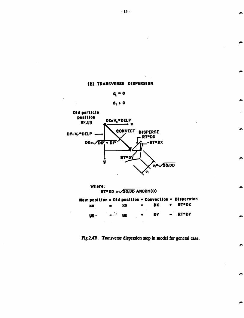
-15-
(B) TRANSVERSE DISPERSION
0
6j>0
Old portfcleposition
xx«uy
DYsVr«DELP
0D=n/DX2.♦ DVZ
DXsVk«DELP
CONVECT disperse/ r- RT»DD
-RT«DX
eisvSd^DD"
Where:
RT«DD ss/SS^ ANORMCO)
New position s Old position ♦ Convection ♦ DispersionXX s XX ♦ DX ♦ RT*DX
uy uu DY - RT«DY
Flg.2.4B. Transveise dispeision step in model for general case.

Old particleposition;
KX^yy
DD=x/WTdV2
-16-
LONGITUDINAL AND
TRANSVERSE DISPERSION
RL*DX
1 «-RT«DVpetition
xx«uv
RL*DV
-RT»DX
RL«DD Bv/Sd[DD ANDRrKO)RT«DD BN/ffd^DD ANORII(O)
Longitudinal TransverseNew position b Old position ♦ Convection ♦ Dispersion t Dispersion
XX « KX ♦ DX ♦ RL»DX ♦ RT«DY
uy »U DY RL-DY RT«DX
Fig.2i. Vector Algebra for di^rsion step.

-17-
If the process described above is repeated for numerous panicles, all having the same
initial position and convective term, a map of the new positions of the panicles can be
created having the discrete density distribution
C(x,r) rt(x) ^ exp4d,vJ
(2.10)
where 4c is the incremental distance over which the N panicles are found and is the total
number of particles in the system. An analogous aigument is used to r^resent the effects
of transverse dispersion as indicated in Fig 2.3B.
Eqs. 2.4, 2.5, and 2.10 are equivalent, with tiie exception that Eqs. 2.4 and 2.5 are
continuous and Eq. 2.10 is discrete. As illustrated in Rg. 2.3A, the distribution of particles
around the mean position, v^Ar, is made to be normally distributed via the fimction
ANORM(p) which produces the number anonn. The fimction ANORMiO) is generated in
the computer code as a simple fimction involving the summation of random numbers.
Probable locations of particles, however, are considered only to 6 standard deviations on
either side of the mean. On a practical basis, the probability of a panicle moving beyond
that distance is very low.
Fig. 2.3B illustrates the extension of the random-walk method to account for disper
sion in a direction transverse to the mean flow. Figs. 2.4A and 2.4B illustrate the algebra
involved when the system is not aligned with the x-y coordinate system. Finally Fig. 2.5
shows both longitudinal and transverse dispersion taking place simultaneously, and the
appropriate vector algebra.- '
22. Model Algorithm
The steps used to implement the concepts described in the preceding section are
described below.
(1) Update the concentrations of each grid block by counting the number of particles in
the given block. For the first time step all concentrations are zero. Note that before
tte start of each simulation, the number of particles required to obtain a unit concen
tration in a grid block is specified.

- 18-
(2) Solve the continiiity equation as shown in Appendix A to obtain the pressure field.
The matrix inversion is done using subroutines ODRV and TDRV from the Yale
package (vectorizedversions of these subroutines are available on the SDSC Cray).
(3) Calculate the velocity field using Darcy*s law and the pressure fidd. The pressures
are known at each node point Thus each velocity is calculated midway between two
consecutive nodes at the block boundary.
(4) Generate the new particles representing the amount of displacing fluid injected during
the current time step. This is done by calculating the number of paiticles correspond
ing to the volume of fluid injected and placing the particles at evenly spaced locations
along die inlet.
(5) Determine current time step. For an explicit solution to be stable, the front cannot
travel more than a distance equivalent to a grid block during a time step. In this
model, the motion of each particle is the sum of a convection step and a dispersion
step. Thus, to avoid having particles travel a distance greater ttian a grid block, the
time step coiresponds to half a grid block traveled at the hi^est existing velocity.
(6) Move new and old panicles as described in Figs. 2.4A and 2.4B. The velocities at
locations other than node points are calculated using the inteipolation scheme shown
in Figs. 2.6A, 2.6B and 2.6C. This is a three step procedure. The first interpolation
(Fig. 2.6A) involves the use of the four intemode velocities in the immediate vicinity
of the x,y position of the particle. The second step (Fig. 2.6B) involves the next
closest four intemode velocities. In the last step (Fig. 2.6C) the final velocity vertors
in the Xand y directions are cMculated. Linear interpolation is in the three steps.
23. Inclusion of Gravity
The random-walk model was modified to include fluids with different densities. The
assumptions made in this second model are:
(1) First contact miscible, incompressible fluids.
(2) (garter power blending rule used to obtain viscosity of mixtures.
(3) Darcy's law applies.

-1
9-
VC
IJ^
)
yC
KiA
O
1-x
-X
1-1
I|4
>1
INT
ER
PO
UT
ION
FUN
CT
ION
SFO
RV
EL
OC
ITY
VE
CT
OR
SB
ET
WE
EN
RO
WS
JA
NO
rj^
l-
J-1
WT
ER
PO
LA
TIO
NFU
NC
TIO
NS
FOR
VaO
CIT
YV
EC
TO
RS
BE
TW
EE
NC
OL
UM
NS
IA
ND
K1
VY•
iyi^
l,J,
1)♦
>
•In
ee:
0.-
1-x
VY
-(1
-x)V
(IA
1)^
*Y
(i+
1,J
tIm
lUrl
y:
VX
.(l-
g)V
(IA
2)*
yY
(l,J
+1
Fig.
2.6A
.Fi
rst
step
inca
lcul
atin
gx
and
yve
loci
tyve
ctor
sfo
rpa
rtic
le.

-20-
VCKJ^
VCK^I
I-*
i-X
1-1 K1
INTERPOLATION FUNCTIONS FORVELOCITV VECTORS BETWEEN
ROWS J AND J-t
J-1
J+1
trrCRPOLATION FUNCTIONS FORmWITY VECTORS BETWEEN
COLUMNS I AND 1-1
Sy• kVCKI ^,1) ♦ (t -*)V(I,JY,1)
sx • «V(0<^1 Xi ♦ (i-y)v(ix,j^)
Fig.2.6B. Second step in calculatingx and y velocity vectors for particle.

-21-
U 1-1
. J-1
r''
xz J*v.0.5
ro.s
«x.
vx
« !-«
INTERPOLATION FUNCTIONS FORKDIRECTION VELOCITY VECTORS
1*1
YZ
J-1
J*1
MTCRPOLATION FUNCTIONS FOR
V DRECTioNvaocmr vectors
FMAL X AND yVaOCITY COMPONENTS:
VY«VY(1-YZ)*Y2.»«
VX«VX(1-XZ)4XZ.*x
Fig.2.6C. Final step in calculating x and y velocity vectors for particle.

-22-
(4) Two dimensional flow (where the second dimension is the vertical direction).
(5) Linear blending method used to obtain densities, of mixtures.
(6) Hamionic weighting used to calculate the transmissibilities.
This model is developed using the same concepts as the linear random-walk model
except that Darcy's law now becomes
where p is the density and g is the gravitational acceleration. As before, the continuity
equation, in conjunction with Darcy*s law, is solved using a point finite difference scheme
as shown in Appendix B. The remainder of &e algorithm proceeds as before, except for
the time step selection criteria which is described below.N
For the calculations with effects of gravity included, the criterion used to calculate the
next time step was changed. In the linear model, the time step is determined as the time
required to flow by convection at the laigest currem vdocity across half a grid block in the
longimdinal direction. This criterion is similar to the stability requirements needed in ordi
nary explicit finite difference fomiulations. In this new model, vertical velocities are much
larger than transverse velocities in the linear model. Also, the grid block size in the vertical
direction is much smaller because of the very narrow models used in the displacement
experiments. This resulted in particles crossing several grid blocks in one time step, and
material balance requirements not being observed. Therefore in the calculations for vertical
cross-sections, the time step was now determined as the time required to flow by convection
at the lai^gest current velocity across half a grid block in any direction. In addition, the par
ticles are allowed to "bounce" off the impermeable boundaries. Results from simulations
run with the first model modified so that particles also bounce off the impemieable boun
daries were not affected due to the small transverse velocities. In the gravity model, parti
cles are allowed to bounce off the impermeable boundaries because without this the solvent
gravity segregation would eventually force most particles to remain near the impemieable
boundaries, resulting in serious material balance errors.
Vp + pg (2.11)

-23-
2.4. Probabilistic Approach
Still another approach was used by King and Scher (1985). Becauseof the promising
qualitative results obtained with this novel approach, the method was investigated for use in
quantitative predictions of finger growth. However, the validation calculations reported in
section 3.3 did not show good agreement with experimental data, and hence this method
was not used in the simulations described in sections 4 and 5. It is nonetheless explained
here as a matter of interest.
It can be shown that a probabilistic interpretation of the fractional flow curve, F, for
immiscible systems reproduces the Buckley-Leverett solution for two-phase flow in one
dimension at^ that a similar interpretation in two dimensions produces viscous instabilities
qualitatively similar to those observed in displacement experiments. In their approach, the
average distance traveled by a particular saturation, 5, is treated as the produa of the dis
tance traveled by fluid moving at the average insterstitial velocity times the probability that
that saturation moves during a time step. This computation scheme reproduces the
Buckley-Leverett velocity of a given fraction if dFldS is chosen as the probability density
limction that governs the choice of a saturation that changes during a time step. The
rationale for this approach is as follows.
The average distance traveled by a specific saturation during a small time interval can
be defined as the product AXgP(S) where P(S) is some [sobability that the saturation S wiU
move during that time interval Axg is the grid block size in the discretization scheme. A
more exact definition ofthis probability is /»[ 5- (dS/l) ^S^S + (d^/2 )]. This is the pro
bability that a saturation S belonging to the interval S ± (dS/2) will move during a specific
time interval. That definition is necessary because for a continuous variable P(S) = 0.
Therefore we can write
PiS) = P s-^&sss+^2 2
-f
f(S)dS (2.12)

-24-
where f{S) is the probability density function of S. This integral, for a veiy small dS, can
be approximated by/(.S) dlS. Therefore A*^(5) becomes (5) dS. From conventional
Buckley-Leverett analysis, a material balance yields
dr dx(2.13)
where F = F(JS) and f is time. (dF/dx) can be written as (dF/dS) (dS/dx\ and since
S = S(x, 0> the exact differential for S is dS = (dS/dt) di + (dS/dx) dx. For a constant
saturation dS-0. Therefore rewriting (dx/dt) as the velocity for a particular saturation front,
gives:
dt= j2_
s ds
Thus in one time interval Ar, the saturation S travels a distance
' ^ dS
(2.14)
(2.15)
This distance can be made dimensionless by dividing both sides by L G^ngth of system).
The following expression is obtained
Ax.'L = ^ ^ = AxL ^ dS dS
dF(2.16)
where Ax is defined as the pore voliunes injected in a time interval. Jt should be noted that
Eq. 2.16 is valid for a specific saturation. Therefore the average distance traveled by
saturations in the range S - (dS/2) ^S^S + (dS/2) that are governed by the above velocity
expression is
AX5 =dS
F(5 +-y)
Ax,dF
ns-^)
dS(2.17)

-25-
This is valid only for very small dS , Taking tfie limit as dS approaches zero (using
I'Hopital's rule for the undefined limit and Leibnitz's rule to obtain the derivative of the
integral) the expression becomes dF. Equating the two egressions for the average dis-
tance traveled by a saturation it can be seen tfiai /(S) dS = dF or /(5) = {dF / dS).
Hence, the probability distribution function of saturation is equal to the derivative of the
fractional flow curve with respect to saturation.
In two dimensions, a similar approach is used. Given a distribution of fluids with
high and low viscosity, the potential flow equation is solved to give the cuirent location of
streamlines. Then, a streamline is chosen randomly, as is the saturation thatchanges during
the time step.

-26-
3. VALIDATION
Several tests were used to validate the random-walk model. First, it was compared to
analytical solutions published in the solute transport literature. Second, ideal miscible dis
placements similar to tfiose used to measure longitudinal and transverse dispersion
coefficients were simulated to determine if the input dispersivities were recovered in the cal
culated Peclet numbers. Finally, displacements in a linear two-dimensional model at vari
ous mobility ratios were simulated and the recoveries compared to e}q)eiimental results
(Blackwell et ai, 1959). The random-walk model that includes gravity was also validated
against experimental results {Blackwell and PozzU 1963).
Simulations done with the model based on the probabilistic inteipretation of the flow
equations were compared to the same experimental results used to validate the linear
random-walk model. Due to the poor qualitative agreem^t between simulation results
obtained with the model and experimental results an attempt to improve the model is
described. Still, the results obtained with this modified model did not agree with experi
mental results and fiie model was dropped from Auther consideratioa
3.1. Random Walk Model
3.1.1. Analytical Solutions
Three different cases were simulated, all with unit mobility ratie and for a homogene-f
ous porous medium.
Case -1- Longitudinal dispersion in uniform one dimensional flow with continuous injec
tion at inlet.
The theoretic^ equation for this case is well known and is presented below. This solution
only applies if the position is not too close to the inlet
C/C„ =^erfc x-vt(3.1)
o
U
U
t = 20 days t = 160 days
till 111111
100 150 200
DISTANCE,feet
J_C
300
Fig. 3.1. Longitudinal dispersion in one dimensional flow with continous injectionat inlet.
to

-28-
In the case studied here, the foUowing parameters were set, D/, =4.5 fflday, v=1fUdas-The transverse dispeisivity was set to zero. Hg. 3.1 shows the results plotted for differenttimes. The numerical solution does ^proximate the analytical one. The matdi can easilybe improved by increasing the number of particles used (in fte case shown it was 100 panicles per grid block) and finer grid mesh (a 3x30 grid was used tore). Note that C/Q >1near the inlet. This is a statistical jiwnomenon, which could be reduced by increasing thenumberof particles injected.
Case -2- Longitudinal dispersion in unifomi one-dimensional flow with a slug of tracerinjected at inlet.
The data for this problem are the same as those used in the previous case. Fig. 3.2 compares the results of this simulation with the theoretical results given by the following equation {Bear, 1972)
N= _-expV47cD5
(x - vt
ADit(3.2)
where is the number of particles times the distance over which particles are counted.
The effects of injecting slugs of increasing numbers of particles are illustrated by comparingFigs. 3.2A. 3.2B and 3.2C.
Case -3- Longitudinal and transverse dispersion in uniform one dimensional flow with aslugof tracer injected at the inlet. -
f
Again, the data for this problem are the same as previously used except that the transversedispeisivity is no longer zero. For this case Dj- X.VIS fp-lday and v= Iftlday. Thetheoretical solution for this case is given by (Fried, 1975)
(X-Vtf y^.Adiyt 4dfvt
where No is the number of particles times the flow rate times the time increment and
and = — and is die number of particles moving with the mean flow. Fig.
(3.3)

40:a
30
20
t=
10da
ys
t=15
0da
ys
10
01
50
20
0
DIS
TA
NC
E,f
eet
Fig.
3.2A
.L
ongi
tudi
nddi
sper
sion
inun
irom
ion
e-di
men
sion
alfl
oww
itha
slug
of
trac
erin
ject
cdat
inle
t(1
00pa
rtic
les)
.

3
10
0II
'I11
IIII
IIII
II[I
IMII
III
IIII
1III
IIIt
III
80
ifti
60
40
t=10
days
t=15
0da
ys
DrS
TA
NC
E,f
eet
Fig.
3.2B
.Lo
ngitu
dina
ldisp
ersio
nin
unifo
rmon
e-di
mcn
siona
lflo
ww
itha
slug
oftra
cer
injc
ctcd
atin
let
(200
part
icle
s).
O

:A.
10
0-
so
t=
10da
ys
t=15
0da
ys
!r
10
0IS
O2
00
DIS
TA
NC
E.f
eet
Fig
.3.2
C.
Lon
gitu
dina
ldi
sper
sion
inun
ifor
mon
e-di
men
sion
alfl
oww
ith
asl
ugo
ftr
acer
inje
cted
atin
let
(300
part
icle
s).
OJ
>3

3qqu»
iti>
sM
1.
&1
S2ics
OQ
fs.3'
§§i
i(L3*
f
fX
Q.
Q.
NumberofParticles
i§IIIIIIIIIIIIIIIIMMIIIIIIIIIIIIIIiIIIMIIIIIIIIII
S-
8-
^-
^I'UJ.
-Zi-

40
0
30
0
u PU *320
0
I 10
0
TT
T1
11
11
11
11
11
1
t=
20da
ys
11
1.1
11
11
11
11
11
iI
i1
11
11
11
11
11
11
-40
-20
20
40
Dis
tanc
eei
ther
side
ofm
ean
flow
(fee
t)
Fig.
3.3B
.L
ongi
tudi
nal
dist
ritn
ition
onbo
thsi
des
of
the
mea
nfl
owaf
ter
20da
ys.

40
0
3
.1'
IIII
IIIM
IIII
IIII
IIIM
IIII
IIII
IIIM
MM
IIII
IIII
TR
AN
SV
ER
SE
DIS
TR
IBU
TIO
N
tB20
days
30
0-
9)
o 1 *SMO I 1
00
—
Illu
jX-4
0-2
00
2040
Dis
tanc
eei
ther
side
ofm
ean
flow
(fee
t)
Fig.3
.3C.
Tran
sver
sedi
strib
utio
non
both
sides
ofth
em
ean
flow
after
20da
ys.

t«70
days
4>to
o
Dis
tanc
eei
ther
side
ofm
ean
flow
(fee
t)
Fig.
3.3D
.L
ongi
tudi
nald
istri
butio
non
both
side
sof
the
mea
nRo
waf
ter7
0da
ys.

1Dui o L
TR
AN
SV
ER
SE
DIS
TR
IBU
TIO
N
t=
70da
ys
ILL
L •60
mU
dOlL
LU
.4
0fi
O
Dis
tanc
eci
ther
side
ofm
ean
flow
(fee
t)
Fig.
3.3E
.T
rans
vers
edi
stri
butio
non
both
side
sof
the
mea
nflo
waf
ter7
0da
ys.

-37-
3.3A shows how the number of particles, at a location 50 feet from the inlet, varies with
time. Thus, after 50 days have elapsed, approximately 140 particles, from an injected slug
of 2000 particles, will be found at 50 feet from flie inlet. Rgs. 3.3B, 3.3C, 3.3D and 3.3E
show the ^reading of the slug of particles in the longitudinal and transverse directions at
two different times. Hence, the agreement between numerical results and theory is excel
lent
3.1.2. Recovery of Input Dispersion Values.
In order to examine how the random-walk models mimics numerically the effects of
dispersion, one dimensional displacements at unit mobility ratio were simulated. Approxi
mate longitudinal Peclet numbers were obtained by fitting calculated effluent composition
data to a straight line in arithmetic probability coordinates. A typical plot is shown in Fig.
3.4A. The longitudinal dispersion coefficient was then extracted from the Peclet number as
follows:
=f (3.4)where v= AOftlday , L, = 6^/, Ly = 2^ and the input Di = 0.14 filday. Fig. 3.4B shows
the range of the calculated dispersion coefficients and its dependence on grid size and seed
number for the random number generator. It can be seen tfiat increasing the number ofgrid
blocks forces the Peclet number obtained from the simulation to converge to the input
value. As the grid size is refined the solution obtained becomes smoother and more accu-
rate, explaining the dependence ofthe recovered Peclet number on the grid size used.
Transverse Peclet numbers were measured by developing code that gimniflted the sand
packed column arrangement {Perkins Johnston, 1963) shown in Fig. 3.5. The
transverse dispersion number was then obtained from the Peclet number in the same manner
described above. The data used were identical to the longimdinal dispereion case discussed
above in addition of Dj = 0.0055 ff-lday.
For both the longitudinal and transverse dispersion cases, the range of values calcu
lated decreased with increasing number ofblocks used and was neariy independent of the

3
U a>
C/i
Ut I
(Xd
-PV
I)/s
qrt(
PVI)
X—
PV
IFi
g,3.
4A.
Plot
ofer
f^(1
-2C
)ve
rsus
—~
=—
.T
hesl
ope
ofth
ere
sulti
nglin
eis
equa
lto
Vm 2
•
u)
oo

1700
1600
^ '500I1§ 1400
H-l
1300
1200
J I I I I I I I I I I I I I I I I I I I I I I I I I I I I I I I I I I I I I I I I I I I I I M I I I I I I I 11
Exact Pe for input data is Pe=1650.* = seed# is 12345.+ = seed # is 34.x = seed# is 516. ♦
» -
' i ' I I I I I4 I I I I I I I I I I I I I I I I I I I 1 I I I I I I I I I I I I IT20 40 60 80 100
Grid Size N (Nx20)
Fig. 3.4B. Longitudinal Pe number as a function of grid size and seed number. N is thenumber of grid blocks in the longitudinal direction.
u>so
>
Fluid B
(r^.Fluid A
Profile along(his line
Fig.3.5. Measuiementof transverse dispersion coefficents.
o

-41 -
seed number used. The ranges varied from about ± 20% for a 30 x 20 grid to about ± 5%
for a 90 X 20 grid in the longitudinal dispersion case. Figs. 3.4 and 3.6 indicate that the
computational scheme used reproduces reasonably well the input values. Thus, the contri
bution of numerical dispersion to the solutions is small provided a sufficioitly fine mesh is
used.
3.13. Comparison with Experimental Results
Blackwell's experiments were carried out to investigate fingering in homogeneous
sands. The results used were those obtained from a sandpack model with dimensions 3/8"
X 24" X 72" at reported flow rates between 30 - 50 ft/day. The sandpack was tested to
assess the homogei^ity of the packing using equal density and viscosity fluids containing
dyes. The results of the assessment also allowed calculation of the effective dispersion
coefficient The values of dispersion coeffici^ts used in these simulations were calculated
using previously derived formulae {Pozzi and BlackwelU 1963) that are given in Appendix F
along with a sample calculation. At a flow rate of AOft!day the calculated dispersion
coefficients were:
Di, = Q.U51fildofDj-= 0.0045
Fig. 3.7 shows the experimental data for four different mobility ratios ranging from 5 to
375, and the results obtained from the simulation runs. The agreement between calculated
and experimental values of the oil recovery is very good. For the mobility ratio of 5, 86f
and 150 a 60x60 grid was used; For flie last mobility ratio case (M=375) a finer grid
(80x60) was needed in order to simulate satisfactorily the experimental results as shown in
Fig. 3.8. Except for grid refinement, no adjustment of input parameters was required to
achieve the agreement shown in Fig. 3.7. This is convincing evidence that the numerical
scheme described represents, with reasonable accuracy, the physical processes that generate
viscous fingers.
It was found throughout this set of simulation runs that the transverse grid resolution
was the dominant factor in obtaining a good match of the experimental results because it

40000
PLi(D
^ 35000
30000
I I I I I 1 M I I I I I I 1 I I I I I I I I I I I I I I I I I I I I I >
Exact Pe for input data is Pe=43200.* = seed # is 12345,+ = seed # is 34.X = seed # is 516.
I « ' I i I I I I I ' » I I ' I » I 1 I I > ' I I I i ' I ' 1 » I I I I20 40
Grid Size N (60xN)
60
Fig. 3.6. Transverse Pe number as a function of grid size and seed number. N is the number ofgrids in the transverse direction.
to

2?OQ
U»
1.
I
vs
ID9
IfA
o
a.
3
PoreVolumeRecovered
NI1IIIIIMMIIIIIMIIIIIIIIMMIIL
^5.SiI;I^
'IIIiIIIIIIIIIIIIIt-
-

-44-
controlled the amount of crossflow between streamlines. Runs were made with even finer
grid meshes (120x60), but the results were unchanged. The number of grids in the longitu
dinal direction did not greatly affect the outcome of the simulations. Additional numerical
experiments showed that the choice of seed number for the random number generator did
not significantly alter the results as ^own in Fig. 3.9 (where two of the curves are almost
identical).
3.1.4. Model Performance Characteristics
One problem with this model is that concentrations greater than unity are possible.
Such behavior is exhibited in Fig. 3.1, where concentrations of 1.1 occur. In the two
dimensional case, concentrations exceeding 2.0 are quite commoa However, they occur
only in the impermeable boundary grid blocks. This behavior can be explained as follows.
Since each injected particle represents a volume of fluid, a grid block can contain only so
many particles before the concentration exceeds unity. Because the dispersion process in
ttie model is random, particles tend to drift into adjacent blocks. In the inner grid blocks,
this behavior is averaged out over time and space and concentrations rarely exceed unity.
However, concentrations greater than unity occur more often in the boundary blocks. It
should be emphasized that these large concentrations last only for one time step. In addi
tion, in a 60x60 grid, such large concentrations occur in two or three grid blocks at most.
There are two reasons for this behavior. First, these blocks are half the size of inner grid
blocks. Secondly, since the boundaries are impermeable, the transverse velocities are small,
thus particles drifting into these blocks will tend to remain there longar. To avoid distortionf
of composition contours, these outer boundary blocks are dropped, in order to obtain
smooth looking lines, when mapping concentration contours. It should be noted that these
outer blocks are included for all other calculations such as determination of characteristic
velocities as presented in sections 4 and 5. Also, concentrations greater than one are
assumed to be one for viscosity calculations.
The behavior described above is dependent on the number of particles use to fill a
grid block. Twenty five particles per grid block were used in die validation runs made to
reproduce Blackwell's experimental data for the M=86 case. Fig. 3.10 shows the recovery

•O 2 Q>
>•
0 1 I s ;> § a.
0.2
0.6
0.4
imn
mii
L♦
=B
lack
wel
l*se
xper
imen
tald
ata
60x6
0~
-
•*
80x6
0:
/
iiM
ilii
iin
iiil
iiir
0.2
0.4
0.6
0.8
PV
I
Fig.
3.8.
Dcp
cndc
ncc
of
rcco
vcry
for
M=3
75on
grid
size
.
1.2
4^

S;
Fig.
3.9.
Dcp
cndc
ncc
ofre
cove
ries
onch
oice
ofse
ednu
mbe
rfo
rM
=86
case
.

-47-
curve obtained using only 10 particles per grid block. It can be seen that the experimental
data is not predicted as well as for the twenty five particles case. Also concentrations in the
boundaiy blocks at a given time step were sometimes greater than nine. Such concentra
tions dropped to about three with25 particles and dropped even further to 1.3 with 100 par
ticles per grid block. It would obviously be ideal to run all cases using 100or more parti
cles per grid block. Unfortunately, this is not feasible because flie model's run time is
directly proportional to the number of particles in the system.
Run times on a Gould 9080 for several cases are shown in Table 3.1. Run time is
also dependent on the mobility ratio, because with a larger mobility ratio a greater number
of iterations is required by the matrix solver at each time step.
When perfbnning the validation runs, good resolution in the transverse direction was
shown to be quite important. An insufficient number of rows results in high velocities
occurring in very few grid blocks, leading to poor agreement with experimental displace
ments. Breakthrough time is not affected by this, but calculated recovery is always much
higher than the experimental recovery.
The random-walk model was modified to handle a quarter five spot geometry. This
model was not validated due to the lack of well documented experimental results. It was
used, however, to find out the effect of grid orientation on the random-walk model. For a
displacement at a mobility ratio of 15 in a homogeneous porous media, it was found that
grid orientation has littleeffect on the recovery as shown in Rg. 3.10B.
3^. Random Walk Model with Gravity *f
The ability of the model to match experimental results {Blackwell andPozzi, 1963) for
displacements in a vertical two-dimensional homogeneous model at various mobility ratios
and gravity numbers is used as the validation criterion. Blackwell*s experiments were car
ried out to investigate the effect of gravity on viscous fingering in homogeneous sands.
The results, which were summarized by plotting the dimensionless solvent penetration
versus pore volume injected (PVI), were obtained by nmning a variety of displacements.
The parameters describing these displacements are given in Table 3.2. These data were
used as the input for the random-walk model described in section 2.2. The dispereion

Match of M=86 case w/10 particles per step
O 0.6
PVI
Fig. 3.10A. Dependence of recovery on number of particles injected per grid block. Simulationresult is shown as solid line.
4^00

Dia
gona
l
oj0
.6P
ara
llel
O0
.4
Fig.
3.10
B.
Eff
ect
of
grid
orie
ntat
ion
onre
cove
ryfo
rM
=15
disp
lace
men
t

-50-
Table 3.1 Run times for simulation of Blackwe11*s viscous fingeringexperiments
Grid Size Mobility Ratio Panicles per block PVI C!PU time(min)
60x60 86 25 1.5 198060x60 86 25 1.0 136060x60 86 100 1.0 483060x60 86 10 1.0 480
60x60 375 25 1.0 174060x60 5 25 1.0 720
120x60 86 25 1.0 357060x40 86 25 1.0 1140

-51-
coefficients for these displacements were calculated as shown in Appendix F. Fig. 3.11
shows the experimental data for five different displacement experiments with mobility ratios
ranging from 1.85 to 69 and gravity numbers ranging from 89 to 200,000, and tiie results
obtained from the random-walk model. The agreement between the calculated and experi
mental values of the solvent penetration is very good. As with the linear model, transverse
grid resolution was very important in obtaining a good match of the e^rimental results.
Runs were made with even finer grids (100x60) but the results remained unchanged. Also,
the choice of seed number for the random number generator did not alter the results. The
gravity model was found to be very sensitive to the flow rate. A five percent decrease in
tfie flow rate resulted in the solvent penetration speeding up by approximately 20%. It
should be noted diat experimental solvent penetration requires estimating some type of
interface between the oil and displacing fluid. In the simulations, the criterion used was a
solvent concentration of 0.05. It was found that this choice gave the best agreement with
the experimental results.
From flow experiments in veitical cross-sectional laboratory models packed with glass
beads {Crane et ai, 1963), it was found that four flow regimes are possible at unfavorable
mobility ratios, depending on the value of the dimensionless group characterizing the ratio
of viscous and gravity forces. This number is:
kgApHNgr =-r^ (3.5)
It is the ratio of the horizontal viscous pressure differential ove» the gravity pressure
differential Stalkup, in his "Miscible Displacement" Monograph (1983) illustrates the
different regimes (Fig. 3.12) and describes them as follows.
At very low values of the gravity number (region I) the displacement is charac
terized by a single gravity tongue overriding the oil The geometry of this
tongue and the vertical sweepout both depend on the particular value of the
gravity number for the displacement. At higher values of the gravity number,
the displacement is still characterized by a single gravity tongue (region II), but
vertical sweepout becomes indeperulent of the particular value of the gravity
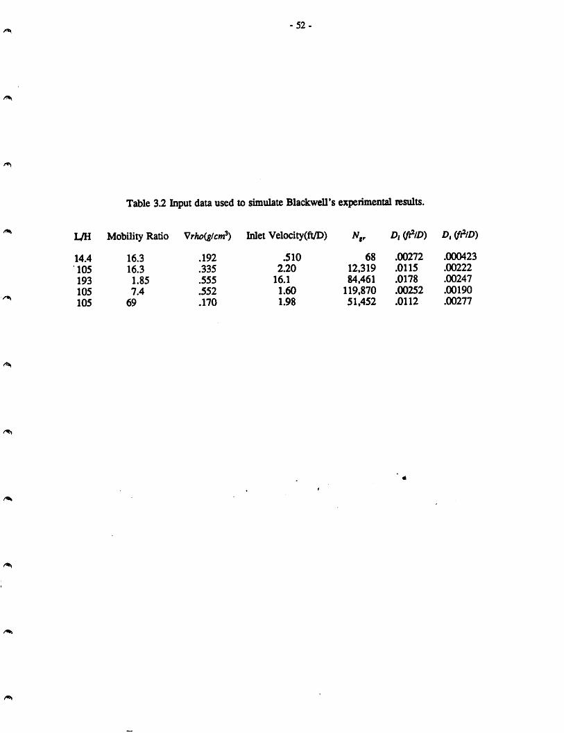
-52-
Table 3.2 Input data used to simulate Blackwell*s experimental results.
L/H Mobility Ratio Vrho(glcn^) Inlet Velocity(ft/I>)
14.4
105
193105105
16.3
16.3
1.857.4
69
.192
.335
.555
352
.170
.5102.20
16.1
1.60
1.98
6812,31984,461
119.87051,452
Di ifilU) D, (ft^lD)
.00272
.0115
.0178
.00252
.0112
.000423
.00222
.00247
.00190
.00277

a00
:j3S«3*ro&a
sIT
e§fi3^a.^Oa=Srt«Ou
§*3g-s
§1
ifg|-
o.2.
ftI
i
1
p.
K>
P__
DimensionlessSolventPenetration
IIMII1IIIIIIIIII[MIIMIIMIIMI1IMIMIIII
IIUIII)II
ssS§ss^
k
111M1111r '«'»•''IIIIIIttIIIIIIIIiIIiIIIIHIIIIIIII
-£S-

-54-
number until a critical value is exceeded. Beyond this critical value, a transition
region is encountered (region III) where secondary fingers form beneath the
main gravity tongue. In this region, sweepoutfor a given value ofPVI increases
sharply with increasing values of the gravity number. Finally, a value of the
gravity number is reached where the displacement is entirely dominated by mul
tiple fingering in the cross section, and vertical sweepout again becomes
independent of the particular value of the gravity number (region VI).
The concentration contours (C=0.05) obtained from the simulations run to validate the verti
cal model axe shown in Fig. 3.13. These contours clearly display the flow regimes
described above. This indicates that the vertical model reproduces the quantitative and the
qualitative features of unstable displacements caused by viscosity and density differences.
33. ProbabUistic Model
A code for one- and two-dimensional calculations has been developed and has been
verified against the results given by King and Scher (1985). The 2-D model can be used to
simulate a quarter five spot or a linear system. Botii immiscible and miscible displacements
can be modeled by using appropriate relative permeability functions.
The approach described in Chapter 2, produces viscous fingers because where low
viscosity fluid replaces high viscosity fluids, streamlines become more closely spaced, and
hence the probability increases that a streamline in that neighborhood will be selected in
subsequent steps increases. Fig. 3.14A ^ows an example of viscous fingers calculated for
miscible displacement with a mobility ratio of 375 in a linear system.^ Hg. 3.14B shows the
distribution of streamlines at the same time (0.15 PV injected). Qearly, the finger at the
lower edge of the flow area is taking most of the injected fluid. It should be noted that in
this method concentrations greater than one do not occur because of the nature of the
method. Only one particle is injected per time step and each particle has a volume equal to
a grid block's volume. Two particles cannot occupy the same grid block.
It is clear from Hg. 3.14 and the plots given by King and Scher (1985) that the
method reproduces many of the qualitative feamres observed in experimental displacements.
However, in attempts to match the experimental results of Blackwell et al. (1958) for

-55-
SOLVENT
region I & ll
SOLVENT
region III
SOLVENT
region IV
Rg. 3.12. Illustration of the different flow regimes (after Stalkup).
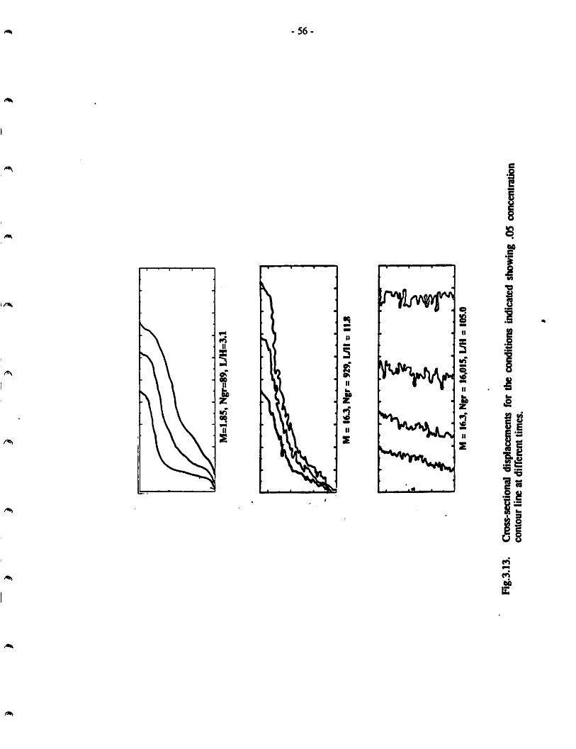
M=
1.85
,Ngr
=:89
,L
/H=
3.1
Ms
I6J,
Ngr
=92
9.M
lr
IIJI
M=
I6J,
Ngr
=i6
,0IS
,L
/H=
lOS.
O
Rg.3
.13.
Cros
s-sec
tiona
ldi
splac
emen
tsfo
rth
eco
nditi
ons
indi
cated
show
ing
.05
conc
entra
tion
con
tou
rli
ne
atd
ifrc
ren
tti
mes
.
o\

-57-
displacements in a linear two-dimensional model at various mobility ratios, the model calcu
lations did not produce reasonably accurate quantitative predictions of displacement perfor
mance. This will be explained subsequently. The experimental data are shown in Fig. 3.15
for a viscosity ratio of 375. In this model, there are two parameters that can be varied,
grid-block size and injection rate. The injection rate is equivalent to a percentage of a
grid-block volume tiiat is added to some grid block at each time step. In the simulations
performed, the breakthrough time could be matched quite easily. However, this did not
mean that the remainder of the curve was also matched. The effect of variations in grid-
block and time-step sizes is also shown in Fig. 3.15. Of the variations examined, changes
in time-step size and in the seed used to start the random number generator for the stream
limction had the largest effects. It should be noted that since changes in the sequence of
random nimibers affect the selection of streamlines and saturations that evolve, any quanti
tative prediction will require the averaging of many runs.
To understand the reasons behind the poor agreement between calculated and meas
ured oil recovery, a more detailed examination was made of the relationship between model
parameters and {^parent longitudinal and transverse dispersion. Because the magnitudes of
physical dispersion contributions have a significant impact on the development of viscous
fingers, it is important to establish whether and how the model mimics numerically the
effects of dispersioa To examine that relation^p, ideal miscible displacements similar to
those used to measure longitudinal and transverse dispersion coefficients were simulated.
Approximate longitudinal Peclet numbers were obtained by fitting calculated effluent com-
position data to a straight line in arithmetic probability coordinates. The longitudinal Peclet
numbers obtained ranged from 10 to 80 and are plotted in Hg. 3.16 versus grid-block size
as a function of time-step size. The results shown in Fig. 3.16 indicate that the level of
numerical dispersion is more sensitive to grid size than to time step size. The time step
size is interpreted as the size of the particle injected into the system. The particle size
represents a volume of fluid equal to a fraction of a grid block volume. Varying this frac
tion between zero and one is equivalent to varying the time step size since different times
will be required to reach the same level of injected fluid.

>
c
a
Fig.
3.14
.Cal
cula
ted
conc
entr
atio
nco
ntou
rs(a
)an
dst
ream
lines
(b)
for
visc
osity
ratio
of
375
at0.
15po
revo
lum
esin
ject
ed.
oo

n -
> «0
is;
S 409
E
(3
-59-
'' i " ' " " " I' " " ' " ' I" " ' In ij 11111 Mn 11111
«*ap.teaM-375
'•ItaaraBrid 16i4l A^yajB^!jO<tadlaMind3«lS3l
« - Mm aoM l<s4t AutfyA^.I teidUSi M3.12Z}!• • iMvaaicl liMI «ia43r«A<*lJ0teidUSI *Hd2-13l
••Mm aoM l<a4l f-ljOteidi .13214 *^3«1223l
" ^ ^ ^ ^ 1111 •..0 02 0.4 0.6 ai 1
Solvent injected(pore volume)
Fig.3.15. Effects ofvariations ofgrid block size as a function of time step.
£
11*5)40
I I I I MII j I I I I I II JI j I1M1U IMI Mx«lSx45(dx^y-.0238}
o-21x63(dx«dy-.0158)
•-29x87(dx-dy«.0n5)
» -
04 06 0.1
Q(%of grid block)
Fig.3.16. Longitudinal Peclel number vs. lime step as afunction of grid blockSize.

-60-
An attempt to measure transverse Peclet numbers was made by developing a code that
simulated the sand packed column arrangement shown in Fig. 3.5 {Perkins and Johnston,
1962). For unit mobility miscible displacement no mixing occurred indicating that no
transverse dispersion is present in this model. That behavior is consistent with the lower
recoveries produced by the model. The reason for the absence of dispersion is that in this
model a saturation contour can only move along a streamlii^. Thus, once a finger breaks
tiiroug^ most of the flow continues throu^ the low resistance path in the finger, and there
is no recovery of material in unswept zones by dispersion into fingers. As a result, no flow
will ever occur between adjacent streamlines.
It is the competition between instability and dispersion that sets finger size in a uni
form porous medium. Thus, model calculations of finger scales are not likely to be quanti
tative unless the model reflects that competition reasonably and accurately. Accordingly,
the model was modified to include transverse mbdng. A transverse step was added in a
maimer similar to the random-walk model. After moving the particle to the location deter
mined by the intersection of the streamline and the concentration contour, that position is
pertuibed in the transverse direction. This is accomplished as shown in Fig. 2.3B. Unfor
tunately as shown in Fig. 3.17, results obtained with this modified version still did not com
pare weU with Blackwell's experimental results. The grid size dependence was not elim
inated as breakthrough time decreased with increasing number of grid blocks. As a result,
this model was dropped from further consideration.
3.4. Summary *
The validation calculations for the random-walk model show good agreement with all
available experimental evidence. It should be pointed out that the agreement for the linear
case is for integrated quantities (recovery). However, the experiments used to validate the
model that includes gravity have some scale information built ia Thus, the random-walk
model seems to be able to handle tiie physical mechanisms resulting fiom the presence of
different length scales. StiU, these validations do not demonstrate explicitly that the calcula
tions resolve the length scale correctly. This question of length scales will be retumed to in
Chapter 6.
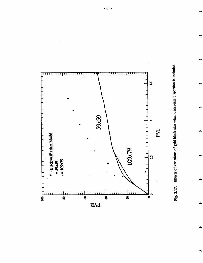
aOQ
-4
I§0•-»»
OQ
§:
fR*
g
1
n
0.
1.§
I
PVR
6SSs%n1111111111111111111111111111111111111[111111111
••*
IIIIIIH^^w
X^NOVO
r^S:CA
III00o\
IIIIIIIIIIIIIIIIIIIIII111IIIIIIItIIIIIIIIIMIIIIII
-19-

-62-
It was also shown that the probabilistic model, even when modified to include
transverse dispersion, does not show good agreement with experimented results. In addition,
the recoveries predicted by this model are strongly dependent on the grid size. As the grid
size used in the simulation increases, breakthrough occurs eariier and recovery decreases.
Thus, the model was dropped from consideration. All the simulations shown in the follow
ing sections were therefore run using the random-walk model.

-63-
4. DISPLACEMENTS IN HOMOGENEOUS POROUS MEDIA
The good agreement between the random-walk model's results and the experimental
results, as described in section 3, shows that it captures many of important physical
mechanisms controlling unstable miscible displacements. Therefore, this model can be used
with some confidence to study the interaction of viscous fingers and heterogeneous porous
media. Thus all the results presented here in the following sections were obtained with the
random-walk model that assumes equal density fluids. Before proceeding, some remaining
questions should be answered concerning unstable displacements in homogeneous porous
media.
These questions are:
(1) How do the viscous fingers propagate at late time ?
(2) How do the concentration contour velocities vary as they move through the
porous media ?
(3) How does the mixing zone behave with time ?
(4) Do the random-walk model predictions agree with linear stability theory?
To answer these questions, a series of simulations was performed with mobility ratios
ranging finom 10 to 100 at flow rates varying between 0.5 and 40 fl/day. A 3/8"x6'x3*
(thickness x width x length) homogeneous model was used. These dimensions, in addition
to the longitudinal and transverse dispersion coefficients are identical to the parameters in
Blackwell's experiments. The resulting Pedet numbers for the base case displacement
(injection rate = 40 fl/day) were 1650 in the longitudinal and 54,000 in flie transverse direc
tion. These are also typical of field scale miscible displacements. This choice was
motivated by the desire to approximate field displacements as closely as possible.
4.1. Late Time Behavior
Figs. 4.1 through 4.9 show the appearance of the resulting viscous fingers and their
evolution with time. For the base case (M=10, (J=40ft/D) shown in Fig. 4.1 at 0.1 PVI,

-64-
approximately ten small fingers coexist. As injection proceeds, the tendency for fingers of
the more mobile fluid to grow in the direction of the pressure gradient of the more viscous
fluid. A finger slightly ahead of its neighbors quickly outruns them and shields them from
liiither growth. Thus at 0.2 PVI, only four fingers remain. At 0.3 PVI, the four previously
existing fingers coalesce to form two laige fingers. Simultaneously, the front of these
fingers spreads and splits into two or more new small fingers. After a split, each new
finger is "stable" as a result of being thinner than the finger from which it split Then as
before, one of these fingers outgrows the others and the whole sequence just described is
repeated. The only difference in the appearance of the concentration contours after 0.3 and
0.6 PVI is that the fingers in the latter are much more elongated. It should be noted that
the spreading, shielding and tip-splitting teiminology has recently been introduced by
Homsy (1987). Similar finger patterns are observed in the displacements with mobility
ratios of 50 (Fig. 4.2) and 100 (Fig. 4.3) nm at the same injection rate.
Lowering the injection rate from 40 ft/day to 10 ft/day, changes the viscous fingering
behavior. Now, at M=10 (Rg. 4.4) and M=50 (Fig. 4.5) the fingers initially formed pro
gress relatively unchanged, their number remaining relatively constant throughout the
length of the displacement In both cases, the finger pattern moves downstream, but the
fingers are no longer growing after approximately 0.3 PVI. There is no further difference
in velocity between fingers and adjacent fluid. On the other hand at the higher mobility
ratio displacement (M=1(X)), the fingers behave like the base case. In the displacements run
at 0.5 fLday injection rate, the fingers that evolved at early times, again remain relatively*
unchanged as they travel through the porous media. The fingers that were fonned are finer
than the ones in the 10 ft/day injection rate case for M=10 and 50. There is also not much
difference in the finger appearance due to changes in the mobility ratio as was observed in
the larger injection rate (v=10 ft/day) displacement
Such behavior is explained by considering the dimensionless transverse dispersion
group
DjL
7^ (4.1)