Embed Size (px)
Citation preview

MIPS Instrument Handbook
Spitzer Heritage Archive Documentation MIPS Instrument and MIPS Instrument Support Teams Version 3, March 2011
MIPS Instrument Handbook
Table of Contents
Chapter 1 Introduction ......................................................................................................... 6
1.1 Document Purpose and Scope ...............................................................................................6 1.2 Basic Definitions .................................................................................................................6 1.3 MIPS Essentials...................................................................................................................7 1.4 Standard Acknowledgements for MIPS Publications ..............................................................8 1.5 How to Contact Us...............................................................................................................8
Chapter 2 Instrument Description....................................................................................... 9
2.1 Overview ............................................................................................................................9 2.2 Description of Optics ...........................................................................................................9
2.2.1 Spatial and Spectral Resolutions ....................................................................................10 2.2.2 Field of View ................................................................................................................11 2.2.3 Point Spread Function...................................................................................................12 2.2.4 Spectral Response .........................................................................................................13 2.2.5 Distortion .....................................................................................................................17
2.3 Detectors ...........................................................................................................................19
2.3.1 Focal Plane Detector Array Design................................................................................19 2.3.2 Detector Performance ...................................................................................................22 2.3.3 Detector Behavior .........................................................................................................24 2.3.4 Annealing and Stimulator Use........................................................................................27
2.4 Electronics ........................................................................................................................27
2.4.1 Hardware .....................................................................................................................27 2.4.2 Software .......................................................................................................................29 2.4.3 Array Control ...............................................................................................................31
2.5 Sensitivity .........................................................................................................................32
2.5.1 Imaging: Sources of Noise and Confusion.......................................................................32 2.5.2 Estimating Background .................................................................................................33 2.5.3 Estimating Signal-To-Noise Ratio and Integration Time ..................................................34 2.5.4 Sensitivity vs. Exposure Time .........................................................................................34 2.5.5 Spectroscopy: Spectral Energy Distribution Sensitivity ....................................................36 2.5.6 Saturation.....................................................................................................................37
Chapter 3 Operating Modes ............................................................................................... 40
3.1 Photometry Mode ..............................................................................................................41
3.1.1 Photometry - 24 µm, Compact Source (Small Field) ........................................................41 3.1.2 Photometry - 24 µm Large Source (Large Field) .............................................................43 3.1.3 Photometry - 70 µm Compact Source (Small Field), Default Pixel Scale ...........................45 3.1.4 Photometry - 70 µm Large Source (Large Field), Default Pixel Scale ...............................48 3.1.5 Photometry - 160 µm, Compact Source (Small Field) ......................................................51 3.1.6 Photometry - 160 µm, Large Source (Large Field) ..........................................................53 3.1.7 Photometry - 160 µm, Enhanced (Small Field) ................................................................54

MIPS Instrument Handbook
3.1.8 Super Resolution Mode..................................................................................................56 3.1.9 Super-Resolution - 70 µm Compact Source (Small Field), Fine Pixel Scale.......................56 3.1.10 Super Resolution - 70 µm Large Source (Large Field), Fine Pixel Scale ...........................58 3.1.11 Super Resolution - 160 µm Compact Source (Small Field) ...............................................59 3.1.12 Total Power (TP) Mode .................................................................................................60 3.1.13 Photometry Raster Map .................................................................................................60
3.2 Large Area Mapping: Scan Mode........................................................................................62
3.2.1 Scan Map Mode ............................................................................................................62 3.2.2 Telescope Motions.........................................................................................................64 3.2.3 Data Acquisition ...........................................................................................................64 3.2.4 Fast Scan Mode ............................................................................................................66
3.3 MIPS/SED Mode ...............................................................................................................66 3.4 Overheads and Best Observing Practices .............................................................................68
3.4.1 Sources of Observing Time Overhead .............................................................................68 3.4.2 Fractional Observing Time Overhead.............................................................................69 3.4.3 Best Observing Practices ...............................................................................................71
Chapter 4 Calibration ......................................................................................................... 73
4.1 Imaging.............................................................................................................................73
4.1.1 Methodology .................................................................................................................73 4.1.2 Photometric Calibration ................................................................................................76 4.1.3 Uncertainties and Repeatability .....................................................................................79 4.1.4 Flat fields .....................................................................................................................79
4.2 Spectroscopy .....................................................................................................................80
4.2.1 Wavelength ...................................................................................................................81 4.2.2 Illumination Correction .................................................................................................82 4.2.3 Flux .............................................................................................................................83 4.2.4 Aperture Correction ......................................................................................................84
4.3 Basic toolset for working with MIPS data............................................................................90
4.3.1 Units and flux densities..................................................................................................90 4.3.2 Flux Conversion Factors ...............................................................................................91 4.3.3 Magnitude Zero Points ..................................................................................................92 4.3.4 Aperture Correction ......................................................................................................93 4.3.5 Color Correction...........................................................................................................97 4.3.6 PSF Characterization ....................................................................................................99 4.3.7 Astrometry - Including Distortion and Pointing............................................................. 100
4.4 Start-Up and Shut-Down Procedures ................................................................................. 101
Chapter 5 Pipeline Processing .......................................................................................... 103
5.1 Level 1: Basic Calibrated Data (BCD) Pipeline .................................................................. 103
5.1.1 Pipeline Updates ......................................................................................................... 103 5.1.2 The MIPS-24 pipeline.................................................................................................. 103 5.2.3 The MIPS-Ge pipeline ................................................................................................. 109
MIPS Instrument Handbook
5.2 Level 2: Post-BCD Pipeline .............................................................................................. 112
5.2.1 MIPS and Pointing Refinement .................................................................................... 113 5.2.2 MIPS and Mosaicking/Outlier Detection....................................................................... 114
Chapter 6 Data Products .................................................................................................. 115
6.1 Data Products Overview ................................................................................................... 115 6.2 File-Naming Conventions................................................................................................. 118
6.2.1 Level 1: BCDs............................................................................................................. 118 6.2.2 Level 2: Post-BCD products ........................................................................................ 118
6.3 Level 1: Basic Calibrated Data (BCD) Products ................................................................. 123
6.3.1 Prime vs. Non-Prime Data ........................................................................................... 123 6.3.2 MIPS/SED BCDs ........................................................................................................ 124 6.3.3 BCD Uncertainties ...................................................................................................... 126 6.3.4 Enhanced BCD (EBCD) Products ................................................................................ 126
6.4 Level 2: Post-BCD Products ............................................................................................. 130
6.4.1 Pipeline Mosaics and Default Spectrum Extraction ....................................................... 130
6.5 Bit Masks ........................................................................................................................ 132 6.6 Header Keywords ............................................................................................................ 137
Chapter 7 Data Features and Artifacts ........................................................................... 140
7.1 MIPS-24 Features and Artifacts ........................................................................................ 140
7.1.1 Pick-off mirror contamination and systematic pointing: practical information ................ 141 7.1.2 Jailbars ...................................................................................................................... 144 7.1.3 Latents ....................................................................................................................... 145 7.1.4 First and second DCE effects ....................................................................................... 149 7.1.5 Post-anneal slow response drift.................................................................................... 150 7.1.6 Bright sources and droop correction ............................................................................ 151 7.1.7 Ghosts and glints ........................................................................................................ 151 7.1.8 Apparent zero-level offset ............................................................................................ 152 7.1.9 Distortions.................................................................................................................. 152 7.1.10 Large- and small-scale gradients ................................................................................. 152 7.1.11 Asteroids! ................................................................................................................... 153
7.2 MIPS Ge: 70 and 160 Micron ........................................................................................... 153
7.2.1 Variations of the slow response .................................................................................... 154 7.2.2 Stim latents ................................................................................................................. 155 7.2.3 Extrapolated or corrupted stim-minus-background measurements.................................. 156 7.2.4 Electronic non-linearities ............................................................................................ 158 7.2.5 Flux non-linearities ..................................................................................................... 158 7.2.6 160 µm short-wavelength light leak .............................................................................. 158 7.2.7 Offline Enhancements to MIPS 70 Fine Scale or 70/160 large-field ................................ 160
Chapter 8 Introduction to Data Analysis ........................................................................ 163
8.1 24 Micron Data................................................................................................................ 163

MIPS Instrument Handbook
8.1.1 Overview and recommended steps for looking at your data ............................................ 163 8.1.2 Self-calibration ........................................................................................................... 163 8.1.3 Sky Background Removal ............................................................................................ 165
8.2 Ge 70 and 160 Micron Data .............................................................................................. 166
8.2.1 High-level summary .................................................................................................... 166 8.2.2 Point vs. extended sources, or why there are 2 BCDs..................................................... 167 8.2.3 The GeRT ................................................................................................................... 169 8.2.4 Recommended steps for looking at your data................................................................. 170 8.2.5 Note on point source photometry .................................................................................. 170 8.2.6 Example: 70 micron faint point source survey ............................................................... 171 8.2.7 Example: 160 micron faint point source survey ............................................................. 173 8.2.8 Example: 70 micron bright extended source.................................................................. 174 8.2.9 Example: 160 micron bright extended source ................................................................ 176
8.3 Making Your Own MIPS SED Mosaics ............................................................................ 178
Appendix A. Version Log ...................................................................................................... 180 Appendix B. Acronyms ......................................................................................................... 181
Appendix C. Pipeline History Log........................................................................................ 186 Appendix D. MIPS BCD File Header .................................................................................. 201 Appendix E. List of Figures .................................................................................................. 207 Appendix F. List of Tables.................................................................................................... 211 Appendix G. Acknowledgements .......................................................................................... 211 Appendix H. Bibliography .................................................................................................... 214
Chapter 1 Introduction
1.1 Document Purpose and Scope
The MIPS Instrument Handbook is one in a series of documents that explain the operations of the Spitzer Space Telescope and its three instruments, the data received from the instruments, and the processing carried out on the data. Spitzer Space Telescope Handbook gives an overview of the entire Spitzer mission and explains the operations of the observatory, while the other three handbooks document the operation of, and the data produced by, the individual instruments (IRAC, IRS and MIPS). The MIPS Instrument Handbook is intended to provide all the information necessary to understand the MIPS standard data products, as processed by Version S18.12 of the online pipeline system, and which are retrievable from the Spitzer Heritage Archive (SHA). Besides the detailed pipeline processing steps and data product details, background information is provided about the MIPS instrument itself, its observational modes and all aspects of MIPS data calibration. It also includes a description of the data acquisition sequences and planning procedures, as an understanding of how and why MIPS data was acquired can be crucial to understanding what to do now that you have data. In this document we present information on the:
• MIPS instrument and its observing modes, • processing steps carried out on the Level 0 (raw) data, • calibration of the instrument, • uncertainties in the data, • final MIPS archival data products.
An overview of the MIPS instrument is given in Chapter 2. In Chapter 3 we discuss the different operating modes which MIPS used to take data. The calibration is described in Chapter 4. Online pipeline processing is described in Chapter 5. The data products themselves are described in Chapter 6. Data features and artifacts are presented in Chapter 7. A brief introduction into MIPS data analysis is given in Chapter 8.
1.2 Basic Definitions
Below are descriptions of the most commonly used terms in this handbook. A complete list of acronyms can be found in Appendix A.
Astronomical Observing Template (AOT): The list of parameters for a distinct Spitzer observing mode. There are 4 possible MIPS AOTs. The Scan Mapping AOT is used to image large areas of the sky in one or more bands nearly simultaneously. The Photometry AOT is used to image sources smaller than about 2 arcminute diameter, including point sources. The Spectral Energy Distribution (SED) AOT is used to

MIPS Instrument Handbook
Introduction 7
MIPS Essentials
obtain low-resolution (R~20) spectra in the 70 µm band. The Total Power (TP) AOT is used to measure the absolute brightness of highly extended emission, e.g., zodiacal light. Each AOT may have a number of modes (for instance, Photometry has 9 and Scan Map has 3) depending on the parameter selection.
Astronomical Observation Request (AOR): The fundamental unit of Spitzer observing. This is an AOT with all of the relevant parameters fully specified. Data Collection Events (DCEs): Single-frame exposures, also referred to as the ''raw'' or Level 0 Data. Basic Calibrated Data (BCD): Also known as Level 1 Data, BCDs are the data products derived from DCEs produced by the processing pipelines. BCDs are designed to be the most reliable product achievable by automated processing. Post-BCD (PBCD): Also known as Level 2 Data or even sometimes Browse Quality Data (BQD), these are data products derived from a full AOR, e.g., a combination of several BCDs. Post-BCD products include (but are not limited to) mosaics, which are produced for both MIPS photometry and scan observations. Automated post-BCD products do not combine data from more than one AOR; observers must do this task themselves (see below). MIPS BCDs and post-BCD products are 2-dimensional FITS images with a full set of header keywords, calibrated in MegaJanskys per steradian (MJy/sr). To convert from MJy/sr to microJy/arcsecond2, multiply by 23.5045. The MIPS pipelines handle the MIPS 24 micron data completely separately from the MIPS 70 and 160 micron data. For this reason, frequently in this manual, the MIPS-24 data, also referred to as ''silicon'' data since the detectors are Si-based (Si:As), are discussed separately from the MIPS 70 and 160 micron data, commonly referred to as ''germanium'' since the detectors are Ge-based (Ge:Ga).
1.3 MIPS Essentials
Please be aware - there are some things you must understand prior to working with MIPS long-wavelength data. The physical nature of the detectors makes fully automated data processing for all types of observations very difficult. Even with the best planning and data pipeline, some detector artifacts will be present in the final processed data. The MIPS 70 and 160 micron channels have Ge:Ga detectors. This material is known to have multiple time constant behaviors when detecting infrared photons, including the MIPS internal calibration stimulators. Please see 2.3.3 for further discussion. In addition, Ge:Ga detectors have response behavior that is different for point source than for extended emission. The pipeline in general cannot deal with these effects. The automated pipelines are very effective in reducing the instrument signatures to a minimum. But, some of the corrections are observation-dependent and, as such, are very difficult to automate. The 70 and 160 micron mosaics provided are intended for quick look analysis only. In general, we do not recommend these be used for detailed science analysis for Ge data. The 24 micron mosaics can, in most cases, be used for detailed analysis, although some care should still be taken. The best automated product produced by the pipelines is the Basic Calibrated Data (BCD) frames. It is critical to understand artifacts (see Chapter 7) that can impact your data and how you might be able to further the

MIPS Instrument Handbook
Introduction 8
Standard Acknowledgements for MIPS Publications
processing of the pipelines to improve your data. Most often you will want to apply some additional corrections to these data that depend on the characteristics of the observation. This Handbook is intended to provide a starting point for such additional reductions. The most relevant software for MIPS data reduction is MOPEX (mosaicking and point source extraction). For the germanium data (70 + 160 µm) one may also find the GeRT (Germanium Reprocessing Tools) valuable for reprocessing the raw data. Documentation for both can be found in the data analysis section of the documentation website. See Chapter 8 for a brief introduction into MIPS data analysis. The separate Data Analysis section of the documentation website provides access to tools, users guides and data analysis recipes.
1.4 Standard Acknowledgements for MIPS Publications
Any paper published based on Spitzer data should contain the following text: ''This work is based [in part] on observations made with the Spitzer Space Telescope, which is operated by the Jet Propulsion Laboratory, California Institute of Technology under a contract with NASA. '' If you received NASA data analysis funding for the research, you should use one of the templates listed under http://irsa.ipac.caltech.edu/data/SPITZER/docs/spitzermission/publications/ackn/. We also ask that you cite at least the seminal MIPS paper (Rieke et al., 2004, ApJS, 154, 25) in your research paper, as well as any other MIPS-related papers where appropriate.
1.5 How to Contact Us
A broad collection of information about the MIPS and MIPS Data Analysis is available on the Spitzer Documentation website: http://irsa.ipac.caltech.edu/data/SPITZER/docs/mips. In addition you may contact us at the helpdesk at http://irsa.ipac.caltech.edu/data/SPITZER/docs/spitzerhelpdesk.
MIPS Instrument Handbook
Instrument Description 9
Overview
Chapter 2 Instrument Description
2.1 Overview
The Multiband Imaging Photometer for Spitzer (MIPS) provides the Spitzer Space Telescope with capabilities for imaging and photometry in broad spectral bands centered nominally at 24, 70, and 160 µm, and for low-resolution spectroscopy between 55 and 95 µm. The instrument contains 3 separate detector arrays each of which resolves the telescope Airy disk with pixels of size or smaller. All three arrays view the sky simultaneously; multiband imaging at a given point is provided via telescope motions. The 24 µm camera provides roughly a 5 ́square field of view (FOV). The 70 µm camera was designed to have a 5 ́square FOV, but a cabling problem compromised the outputs of half the array; the remaining side (''side A'') provides a FOV that is roughly 2.5 ́by 5 .́ The 160 µm array projects to the equivalent of a 0.5 ́by 5 ́FOV and fills in a 2 ́by 5 ́ image by multiple exposures. The 70 µm array also has a narrow FOV/higher magnification mode, and is additionally used in a spectroscopic mode. The MIPS cryogenic scan mirror mechanism (CSMM) is integral to all observational operations, allowing selection of different optical trains, image motion compensation during scanned imaging, and one dimensional image dithering. A brief, high-level summary of MIPS for astronomers appears in the ApJS Spitzer Special Issue, specifically the paper by Rieke et al. (2004, ApJS, 154, 25) entitled ''The Multiband Imaging Spectrometer for Spitzer.'' A copy of this paper is available on the website.
2.2 Description of Optics
MIPS employs three distinct array detectors (128x128 pixel Si:As BIB; 32x32 pixel Ge:Ga; 2x20 pixel stressed Ge:Ga) to provide high-sensitivity, low-noise, diffraction-limited performance from roughly 20 µm to 180 µm. The short-wavelength Si:As array is combined with a permanent filter to give a bandpass from 20.8 to 26.1 µm with a weighted average wavelength of 23.68 µm. The Ge:Ga array is combined with a filter to give a bandpass from 61 to 80 µm with a weighted average wavelength of 71.42 µm for imaging. This array can also be used in conjunction with a slit and grating to provide low-resolution ( ) spectroscopy from 55-95 µm in Spectral Energy Distribution (SED) mode. The 2x20 stressed Ge:Ga array is combined with a permanent filter to give a bandpass from 140 to 174 µm with a weighted average wavelength of 155.9 µm. The pixel size for all 3 arrays is roughly to sample the telescope Airy pattern fully. In addition, a fine pixel scale/narrow FOV can be selected for use with the 70 µm band to provide higher spatial resolution than is possible with the nominal pixel scale, but at a somewhat degraded sensitivity. Selection between the various bands and modes of operation is accomplished through the cryogenic scan mirror, which deflects incoming light into the desired optical path. The scan mirror is also used for image motion compensation during mapping operations, and provides chopping between source and sky to improve the accuracy of the MIPS long wavelength photometry (Rieke, 2004).
MIPS Instrument Handbook
Instrument Description 10
Description of Optics
2.2.1 Spatial and Spectral Resolutions
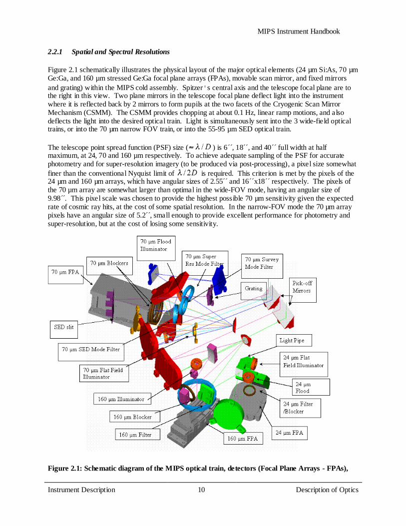
Figure 2.1 schematically illustrates the physical layout of the major optical elements (24 µm Si:As, 70 µm Ge:Ga, and 160 µm stressed Ge:Ga focal plane arrays (FPAs), movable scan mirror, and fixed mirrors and grating) within the MIPS cold assembly. Spitzer's central axis and the telescope focal plane are to the right in this view. Two plane mirrors in the telescope focal plane deflect light into the instrument where it is reflected back by 2 mirrors to form pupils at the two facets of the Cryogenic Scan Mirror Mechanism (CSMM). The CSMM provides chopping at about 0.1 Hz, linear ramp motions, and also deflects the light into the desired optical train. Light is simultaneously sent into the 3 wide-field optical trains, or into the 70 µm narrow FOV train, or into the 55-95 µm SED optical train. The telescope point spread function (PSF) size ( ) is 6´ ,́ 18´´, and 40´ ́full width at half maximum, at 24, 70 and 160 µm respectively. To achieve adequate sampling of the PSF for accurate photometry and for super-resolution imagery (to be produced via post-processing), a pixel size somewhat finer than the conventional Nyquist limit of is required. This criterion is met by the pixels of the 24 µm and 160 µm arrays, which have angular sizes of 2.55´ ́and 16´´x18´ ́respectively. The pixels of the 70 µm array are somewhat larger than optimal in the wide-FOV mode, having an angular size of 9.98´́ . This pixel scale was chosen to provide the highest possible 70 µm sensitivity given the expected rate of cosmic ray hits, at the cost of some spatial resolution. In the narrow-FOV mode the 70 µm array pixels have an angular size of 5.2´ ,́ small enough to provide excellent performance for photometry and super-resolution, but at the cost of losing some sensitivity.
Figure 2.1: Schematic diagram of the MIPS optical train, detectors (Focal Plane Arrays - FPAs),

MIPS Instrument Handbook
Instrument Description 11
Description of Optics
and optical paths. Two mirror facets are attached to the Cryogenic Scan Mirror Mechanism (CSMM): one mirror feeds the 70 µm optical train (normal FOV, narrow FOV and spectrometer/SED), while the second mirror feeds both the 24 µm and 160 µm optical trains. The CSMM provides chopping and one-dimensional dithering for all 3 arrays as well as selecting among the various bands and modes.
The Spectral Energy Distribution (SED) mode utilizes a 3.8´x0.32 ́slit to produce low-resolution (R=15-25) spectroscopy covering a wavelength range of 52-97 µm. As half of the original array has significantly higher noise, the usable length of the spectroscopic slit is actually about 2 .́ The SED slit was originally designed to be offset with respect to the array such that an 8x32 portion of the array is unilluminated in SED mode. This strip was supposed to provide a dark measurement for the 70 µm array when taking measurements in TP mode; the other two arrays can be put in the dark by suitable positioning of the scan mirror. This special treatment for the 70 µm array in TP mode is required because of the multiple 70 µm optical paths which might allow light to contaminate the dark measurement. Unfortunately, this region falls on side B of the 70 µm array, i.e., the noisier side. Therefire the TP mode used side A only, chopping between the sky position and an internal dark position.
2.2.2 Field of View
All three arrays simultaneously view non-overlapping fields on the sky. The 24 µm array has a ~5 ́square field of view; roughly 8 ́away is the 70 µm array. The 70 µm array suffers from thermally-activated high resistance in a cable connection that is external to the instrument, but feeds it. This has resulted in significantly increased noise on side B of the array, rendering that side essentially unusable. Also, one readout on side A (located in the lower right corner in data oriented as observers receive it, next to side B) is inoperative; the resulting shape (roughly 2.5´x5 )́ can be seen in 70 µm bad pixel mask (see section 6.5). Basic parameters of interest for MIPS are summarized in Table 2.1.
Table 2.1: MIPS principal optical parameters.
Band Mode Array Format
Pointed FOV (arcmin)
Pixel Size (arcsec)
(µm)
F/#
24µm Imaging 128x128 5.4x5.4 2.49x2.60 23.7 7.4 4.7µm
70µm Wide FOV 32x32 5.2x2.6 9.85x10.06 71 18.7 19 µm
70µm Narrow FOV/ Super R
32x32 2.7x1.35 5.24x5.33 71 37.4 19 µm
70µm SED 32x241 2.7x0.342 9.8 55-953
18.7 1.7 µm/px
160µm Imaging 2x20 5.3x2.14 15.96x18.04 156 46 35 µm
1 Note that full spectral coverage is limited to only 32x12 because of the dead 70 µm readout and the noisy side B.

MIPS Instrument Handbook
Instrument Description 12
Description of Optics
2 Slit width is 2 pixels, slit length is 16 pixels; note that full spectral coverage is only obtained over a 2.0´ length of the slit because of the dead 70 µm readout. 3 Because of a bad readout at one end of the slit, the spectral coverage for 4 columns of the array is reduced to about 65-106 µm. 4 Includes scan motion required to sample PSF fully. Single frame FOV is 5.3x0.5 arcminutes. In a single pointing, the 160 µm array views two 5.3 ́by 16´ ́strips separated by a 16´́ wide blank strip giving a 5.3´x0.75 ́unfilled FOV. The central blank strip of the 160 µm array is filled by taking images at interleaved scan positions. One block of 5 contiguous pixels in the 160 µm array exhibits anomalous behavior attributable to a thermally-activated short in cabling external to MIPS but well inside the Cryogenic Telescope Assembly. In data oriented as observers receive it, this block is located in the bottom row; it is the third group of 5 pixels in from the left. The ''bite'' taken out of the array is visible in the 160 µm bad pixel mask (see section 6.5). These pixels are not quite square at 16´´x18´ .́ Occasionally for brevity, we refer to these pixels as 16´ ́square with the knowledge that they are slightly rectangular.
2.2.3 Point Spread Function
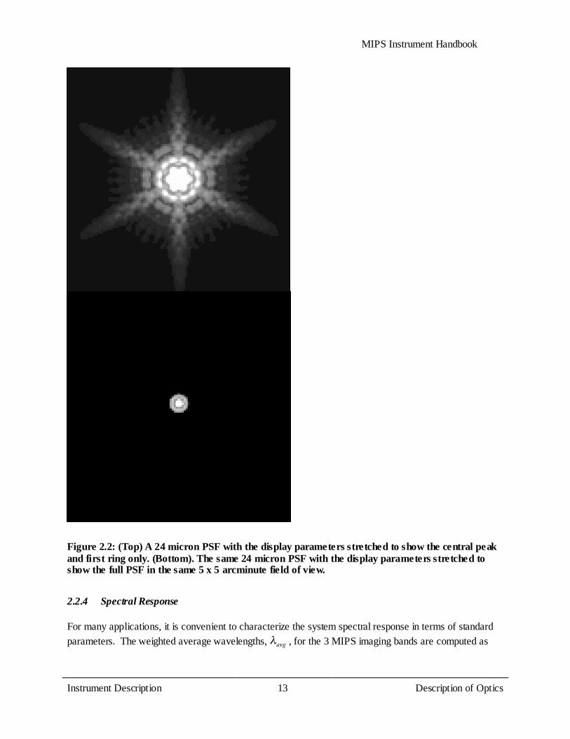
MIPS delivered diffraction-limited imaging capability at all three wavelengths due to the matching of the pixel scales to the width of the Spitzer PSF. In the wide field of view mode at 70 microns the pixels are slightly too large to achieve lambda/2D sampling of the PSF, so observers who were particularly interested in getting the highest possible spatial resolution at 70 microns should have utilized the narrow field of view (''super resolution'') mode. In addition, image quality at the corners of the 24 micron field of view is slightly degraded. Off-center variation in PSF only applies to the 24 micron band models, and not to the longer wavelength bands. Variations of the PSF over the array in the 70 and 160 micron model images appear to be negligible Figure 2.2 is an example of the 24 micron PSF at the array center (T = 5000 K). The PSF is strongly centrally peaked with a well defined first Airy ring. For bright astronomical sources with a very high signal-to-noise ratio, the full extent of the PSF might be visible in the MIPS images. The telescope secondary mirror support ''spiders'' result in the radially extending artifacts in the PSF. We note that these images are theoretical, Tiny Tim PSFs and not actual data. The model PSFs are very close to the measured in-orbit PSFs. The point spread function (PSF) in the MIPS bands is not highly sensitive to small changes or differences in telescope and instrument optical parameters. The MIPS PSF images are dominated by the telescope optics, not the internal instrument optics.
MIPS Instrument Handbook
Instrument Description 13
Description of Optics
Figure 2.2: (Top) A 24 micron PSF with the display parameters stretched to show the central peak and first ring only. (Bottom). The same 24 micron PSF with the display parameters stretched to show the full PSF in the same 5 x 5 arcminute field of view.
2.2.4 Spectral Response
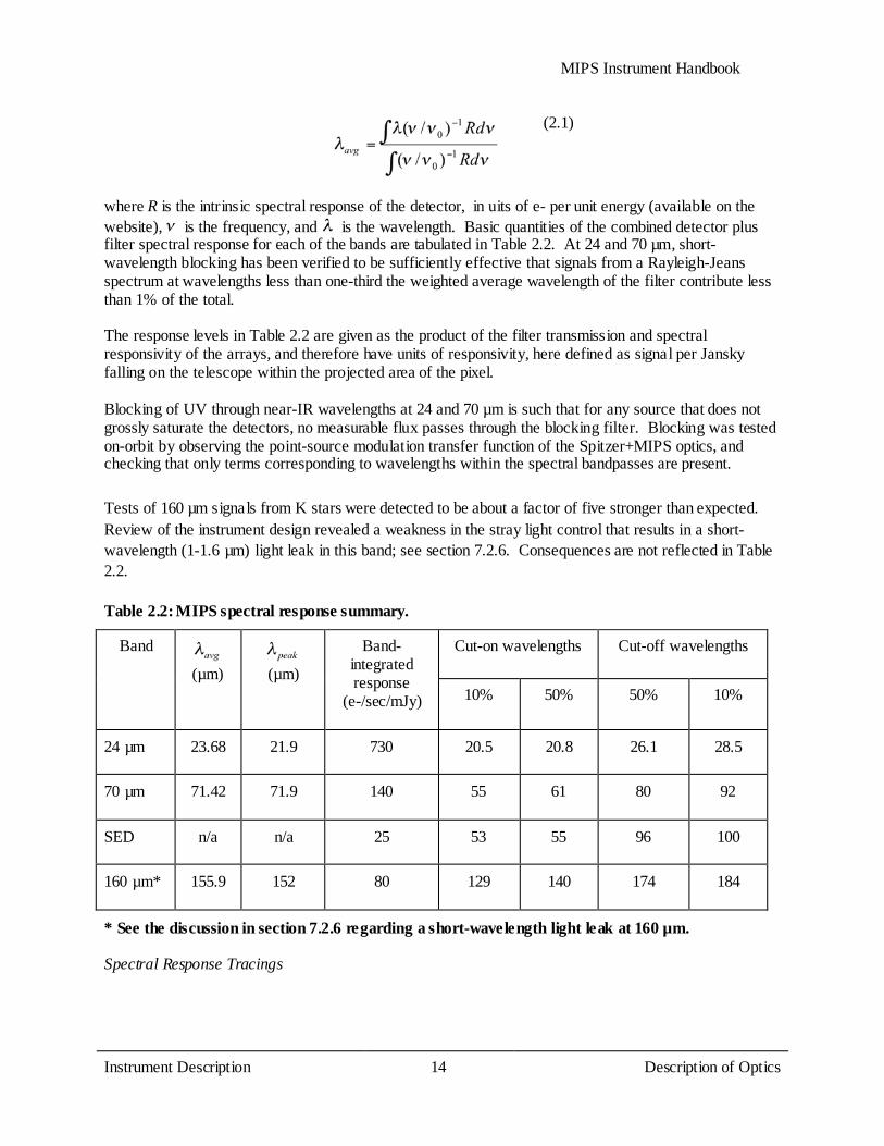
For many applications, it is convenient to characterize the system spectral response in terms of standard parameters. The weighted average wavelengths, , for the 3 MIPS imaging bands are computed as
MIPS Instrument Handbook
Instrument Description 14
Description of Optics
(2.1)
where R is the intrinsic spectral response of the detector, in uits of e- per unit energy (available on the website), is the frequency, and is the wavelength. Basic quantities of the combined detector plus filter spectral response for each of the bands are tabulated in Table 2.2. At 24 and 70 µm, short-wavelength blocking has been verified to be sufficiently effective that signals from a Rayleigh-Jeans spectrum at wavelengths less than one-third the weighted average wavelength of the filter contribute less than 1% of the total. The response levels in Table 2.2 are given as the product of the filter transmission and spectral responsivity of the arrays, and therefore have units of responsivity, here defined as signal per Jansky falling on the telescope within the projected area of the pixel. Blocking of UV through near-IR wavelengths at 24 and 70 µm is such that for any source that does not grossly saturate the detectors, no measurable flux passes through the blocking filter. Blocking was tested on-orbit by observing the point-source modulation transfer function of the Spitzer+MIPS optics, and checking that only terms corresponding to wavelengths within the spectral bandpasses are present.
Tests of 160 µm signals from K stars were detected to be about a factor of five stronger than expected. Review of the instrument design revealed a weakness in the stray light control that results in a short-wavelength (1-1.6 µm) light leak in this band; see section 7.2.6. Consequences are not reflected in Table 2.2.
Table 2.2: MIPS spectral response summary.
Band (µm)
(µm)
Band-integrated response
(e-/sec/mJy)
Cut-on wavelengths Cut-off wavelengths
10% 50% 50% 10%
24 µm 23.68 21.9 730 20.5 20.8 26.1 28.5
70 µm 71.42 71.9 140 55 61 80 92
SED n/a n/a 25 53 55 96 100
160 µm* 155.9 152 80 129 140 174 184
* See the discussion in section 7.2.6 regarding a short-wavelength light leak at 160 µm.
Spectral Response Tracings
MIPS Instrument Handbook
Instrument Description 15
Description of Optics
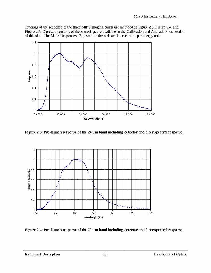
Tracings of the response of the three MIPS imaging bands are included as Figure 2.3, Figure 2.4, and Figure 2.5. Digitized versions of these tracings are available in the Calibration and Analysis Files section of this site. The MIPS Responses, R, posted on the web are in units of e- per energy unit.
Figure 2.3: Pre-launch response of the 24 µm band including detector and filter spectral response.
Figure 2.4: Pre-launch response of the 70 µm band including detector and filter spectral response.
MIPS Instrument Handbook
Instrument Description 16
Description of Optics
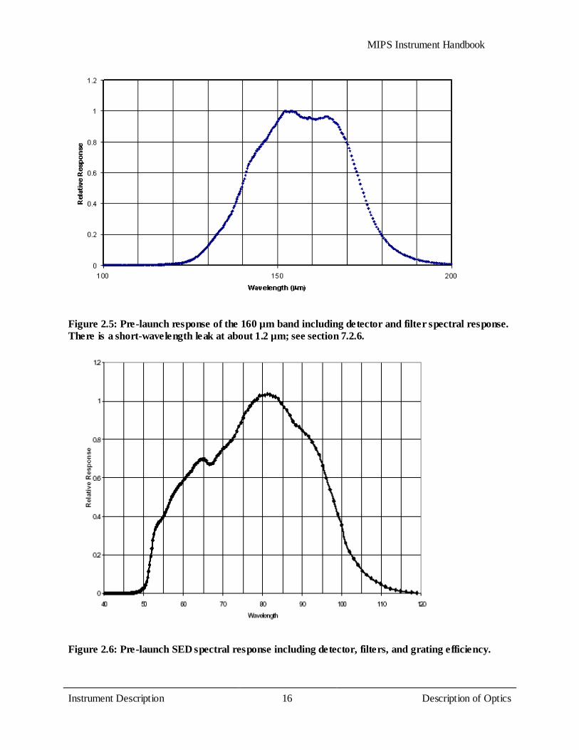
Figure 2.5: Pre-launch response of the 160 µm band including detector and filter spectral response. There is a short-wavelength leak at about 1.2 µm; see section 7.2.6.
Figure 2.6: Pre-launch SED spectral response including detector, filters, and grating efficiency.
MIPS Instrument Handbook
Instrument Description 17
Description of Optics
Spectral Energy Distribution (SED) Mode
The spectral response of MIPS in the Spectral Energy Distribution (SED) mode was determined pre-flight using test filters and a far-IR blackbody source. A tracing of the SED mode spectral response is in Figure 2.6; basic performance is given in Table 2.1 and Table 2.2. The slit for the SED mode is 2 pixels wide and 24 pixels long; however, 8 of those 24 pixels fall on side B (the noisy side) of the array. Moreover, another 4 pixels have incomplete spectral coverage due to the bad readout on side A. The resulting slit length giving complete spectral coverage is thus 12 pixels. The grating disperses the light parallel to the direction of motion of the scan mirror; CSMM motions are used to switch between object and sky positions, while spacecraft pointing is used to move the object between positions in the slit. The spectrum is dispersed by a reflection grating across 32 pixels, and covers the wavelength range from 55 to 95 µm, giving a nominal dispersion per pixel-pair of 3.4 µm. The resultant spectral resolution, , is 15 at 52 µm, about 24 at 80 µm, and about 25 from 85 µm to the long wavelength cutoff.
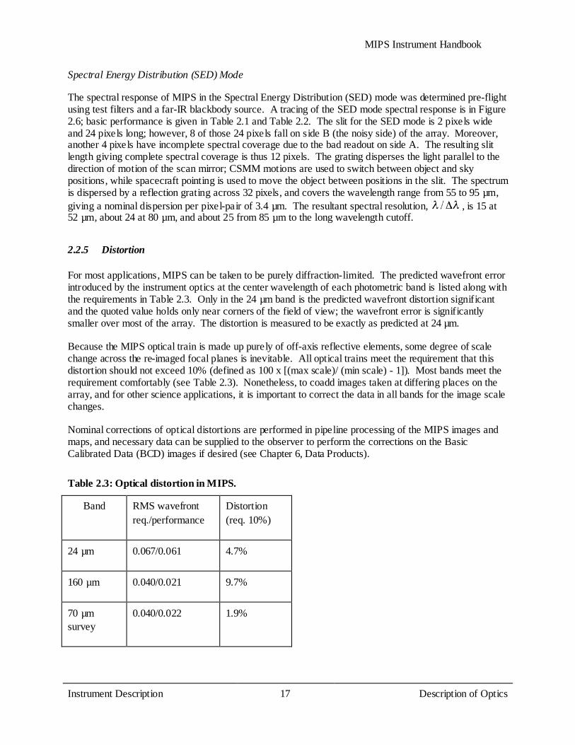
2.2.5 Distortion
For most applications, MIPS can be taken to be purely diffraction-limited. The predicted wavefront error introduced by the instrument optics at the center wavelength of each photometric band is listed along with the requirements in Table 2.3. Only in the 24 µm band is the predicted wavefront distortion significant and the quoted value holds only near corners of the field of view; the wavefront error is significantly smaller over most of the array. The distortion is measured to be exactly as predicted at 24 µm. Because the MIPS optical train is made up purely of off-axis reflective elements, some degree of scale change across the re-imaged focal planes is inevitable. All optical trains meet the requirement that this distortion should not exceed 10% (defined as 100 x [(max scale)/ (min scale) - 1]). Most bands meet the requirement comfortably (see Table 2.3). Nonetheless, to coadd images taken at differing places on the array, and for other science applications, it is important to correct the data in all bands for the image scale changes. Nominal corrections of optical distortions are performed in pipeline processing of the MIPS images and maps, and necessary data can be supplied to the observer to perform the corrections on the Basic Calibrated Data (BCD) images if desired (see Chapter 6, Data Products).
Table 2.3: Optical distortion in MIPS.
Band RMS wavefront req./performance
Distortion (req. 10%)
24 µm 0.067/0.061 4.7%
160 µm 0.040/0.021 9.7%
70 µm survey
0.040/0.022 1.9%

MIPS Instrument Handbook
Instrument Description 18
Description of Optics
70 µm super resolution
0.040/0.021 7.5%
70 µm SED 0.040/0.022 4.1%
Scan Alignment
Scan Map Mode operation requires the use of the MIPS scan mirror to compensate for image motion during Spitzer spacecraft continuous scan motion. The desired result is the simultaneous delivery of a succession of stationary sky images to all MIPS Focal Plane Arrays (FPAs). Ideally the spacecraft slews its view vector along a straight line in object space (able to be oriented to MIPS needs) at a constant angular velocity, while the MIPS scan mirror moves at a constant angular velocity (to which the spacecraft rate can be matched). Given an ideal optical system, the full-field images will remain fixed on the FPAs for the duration of the integrations. The actual instrument departs slightly from these ideal conditions. There are two general classes of image smear due to the scan mirror motions:
1. Image smear sources in individual bands a. Departures from constant angular velocity. b. Changes in field distortion or magnification during scan motion.
2. Image smear sources as a result of a mismatch between bands a. Angular magnification mismatch between the sides of the instrument at the scan mirror. b. Direction of image motion mismatch between sides of the instrument.
Analysis of scan mirror operation during instrument tests indicates that all of these sources of image smear should lie well within the FWHM of the diffraction limited image, and for most observing modes should be virtually undetectable in the observed shape of the PSF. The one minor exception is in the scan map mode at the fast scan rate where a slight elongation of the images may occur due to sources of type 2, which cannot be reconciled through adjusting the spacecraft motion or the scan mirror action. The mismatch may become apparent in this mode because of the relatively long throw over which the scan mirror is used to freeze the image motion.
Ghost Images
Reflections from filters in front of focal plane arrays frequently cause ghost images. In the case of the 160 µm band, it has been possible to tilt the bandpass filter far enough so that no ghosts will occur, but at 24 and 70 µm very faint, slightly out-of-focus ghost images do appear. The intensity of the ghost images measured during tests of the integrated MIPS is 0.5% of the brightness of the primary image at 24 µm, and is 2% of the brightness of the primary image at 70 µm. The single ghost image formed on the 70 µm array is 6 pixels (in wide-FOV mode) from the primary image.

MIPS Instrument Handbook
Instrument Description 19
Detectors
2.3 Detectors
2.3.1 Focal Plane Detector Array Design
Si:As (24 µm) Array
The MIPS 24 µm array was developed and furnished to MIPS through the Spitzer InfraRed Spectrograph (IRS) program. It is a Boeing 128x128 pixel blocked impurity band (BIB) Si:As device identical to those in the two short wavelength spectrometers of IRS except that the MIPS array has an anti-reflection coating optimized for the 24 µm region. The device has four output amplifiers, each of which reads every fourth pixel in a row. That is, the readout is in columns, with an output amplifier for each of columns 1, 2, 3, and 4, repeated for columns 5, 6, 7, and 8. The array is described in more detail by van Cleve (1995; Proc. SPIE Vol. 2553, p. 502) and in the IRS Instrument Manual, as well as Houck et al. (2004, ApJS, 154, 18). A summary of the characteristics of the flight array is given in Table 2.4.
Figure 2.7: 70 µm array 4x32 submodule.
Ge:Ga (70 and 160 µm) Arrays
The 70 µm and 160 µm arrays both utilize traditional gallium-doped germanium extrinsic photoconductor detector technology. Because many of the performance characteristics of the two arrays are very similar, the performance of both is discussed below, after the physical layout of the two arrays is described. Differences between the performance of the two arrays are pointed out as needed.
70 µm Array Design
The 70 µm array is described by Young (1998; Proc. SPIE Vol. 3354, p. 57-65). Figure 2.7 shows a single 4x32 pixel subarray module from the 70 µm array. Each row of 32 pixels is fabricated from a single 24 mm x 0.5 mm x 2 mm piece of Ge:Ga. The 24 mm length is divided into 32 pixels by photolithography, yielding a dimension of 0.75 mm x 0.5 mm for the illuminated face of each pixel. Absorption of photons occurs over the 2 mm depth of the pixel and is enhanced by a mirror at the back of the pixel that directs transmitted photons back through the sensitive volume. Individual rows are separated by spaces of 0.25 mm. Wedge-shaped germanium optical concentrators are placed in front of
MIPS Instrument Handbook
Instrument Description 20
Detectors
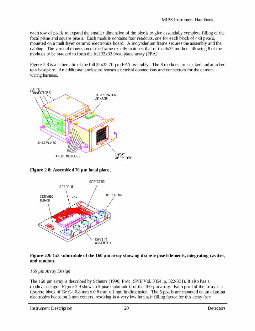
each row of pixels to expand the smaller dimension of the pixels to give essentially complete filling of the focal plane and square pixels. Each module contains four readouts, one for each block of 4x8 pixels, mounted on a multilayer ceramic electronics board. A molybdenum frame secures the assembly and the cabling. The vertical dimension of the frame exactly matches that of the 4x32 module, allowing 8 of the modules to be stacked to form the full 32x32 focal plane array (FPA). Figure 2.8 is a schematic of the full 32x32 70 µm FPA assembly. The 8 modules are stacked and attached to a baseplate. An additional enclosure houses electrical connections and connectors for the camera wiring harness.
Figure 2.8: Assembled 70 µm focal plane.
Figure 2.9: 1x5 submodule of the 160 µm array showing discrete pixel elements, integrating cavities, and readout.
160 µm Array Design
The 160 µm array is described by Schnurr (1998; Proc. SPIE Vol. 3354, p. 322-331). It also has a modular design. Figure 2.9 shows a 5-pixel submodule of the 160 µm array. Each pixel of the array is a discrete block of Ge:Ga 0.8 mm x 0.8 mm x 1 mm in dimension. The 5 pixels are mounted on an alumina electronics board on 3 mm centers, resulting in a very low intrinsic filling factor for this array (see
MIPS Instrument Handbook
Instrument Description 21
Detectors
below). Also attached to the board are a single readout for the 5 pixels and an array of 5 integrating cavities.
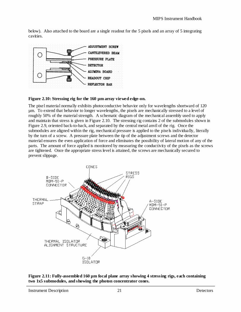
Figure 2.10: Stressing rig for the 160 µm array viewed edge-on. The pixel material normally exhibits photoconductive behavior only for wavelengths shortward of 120 µm. To extend that behavior to longer wavelengths, the pixels are mechanically stressed to a level of roughly 50% of the material strength. A schematic diagram of the mechanical assembly used to apply and maintain that stress is given in Figure 2.10. The stressing rig contains 2 of the submodules shown in Figure 2.9, oriented back-to-back, and separated by the central metal anvil of the rig. Once the submodules are aligned within the rig, mechanical pressure is applied to the pixels individually, literally by the turn of a screw. A pressure plate between the tip of the adjustment screws and the detector material ensures the even application of force and eliminates the possibility of lateral motion of any of the parts. The amount of force applied is monitored by measuring the conductivity of the pixels as the screws are tightened. Once the appropriate stress level is attained, the screws are mechanically secured to prevent slippage.
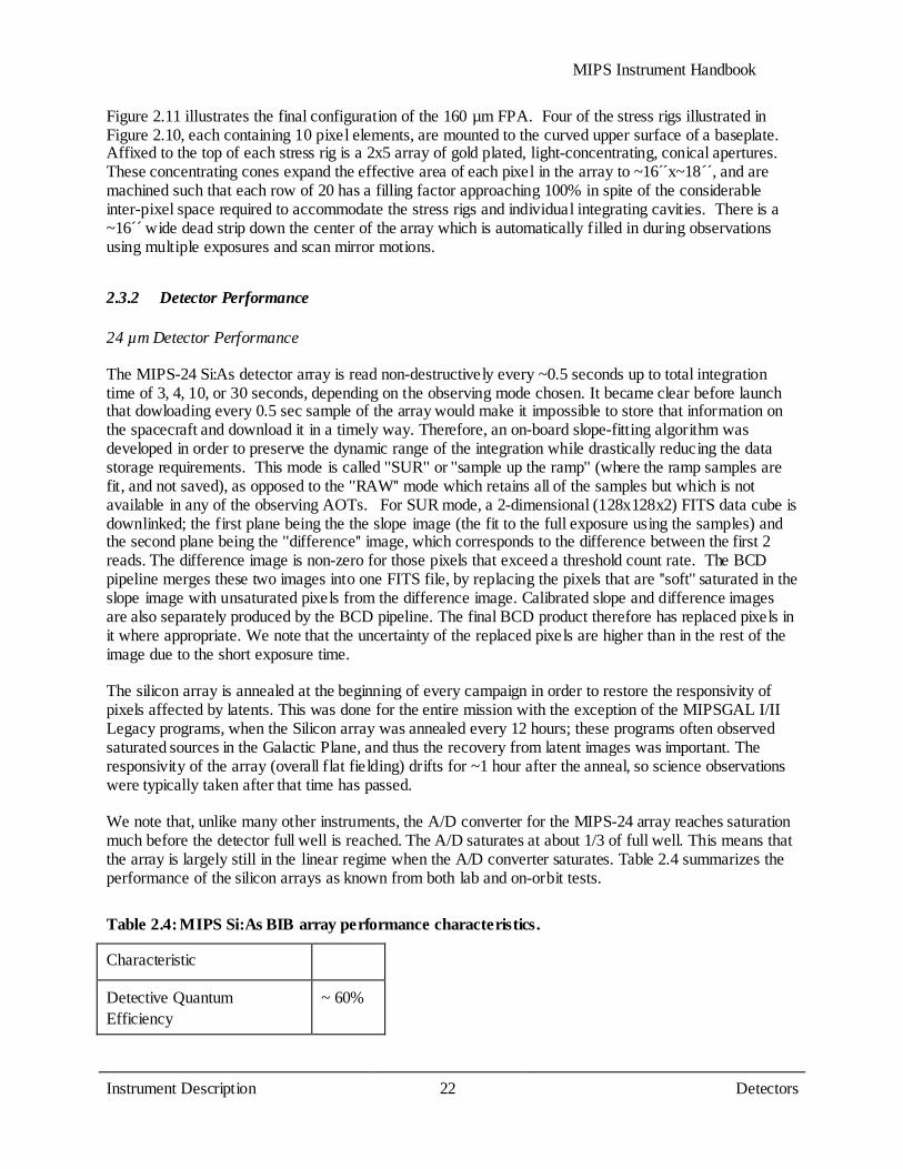
Figure 2.11: Fully-assembled 160 µm focal plane array showing 4 stressing rigs, each containing two 1x5 submodules, and showing the photon concentrator cones.
MIPS Instrument Handbook
Instrument Description 22
Detectors
Figure 2.11 illustrates the final configuration of the 160 µm FPA. Four of the stress rigs illustrated in Figure 2.10, each containing 10 pixel elements, are mounted to the curved upper surface of a baseplate. Affixed to the top of each stress rig is a 2x5 array of gold plated, light-concentrating, conical apertures. These concentrating cones expand the effective area of each pixel in the array to ~16´́ x~18´´, and are machined such that each row of 20 has a filling factor approaching 100% in spite of the considerable inter-pixel space required to accommodate the stress rigs and individual integrating cavities. There is a ~16´ ́wide dead strip down the center of the array which is automatically filled in during observations using multiple exposures and scan mirror motions.
2.3.2 Detector Performance
24 µm Detector Performance
The MIPS-24 Si:As detector array is read non-destructively every ~0.5 seconds up to total integration time of 3, 4, 10, or 30 seconds, depending on the observing mode chosen. It became clear before launch that dowloading every 0.5 sec sample of the array would make it impossible to store that information on the spacecraft and download it in a timely way. Therefore, an on-board slope-fitting algorithm was developed in order to preserve the dynamic range of the integration while drastically reducing the data storage requirements. This mode is called ''SUR'' or ''sample up the ramp'' (where the ramp samples are fit, and not saved), as opposed to the ''RAW'' mode which retains all of the samples but which is not available in any of the observing AOTs. For SUR mode, a 2-dimensional (128x128x2) FITS data cube is downlinked; the first plane being the the slope image (the fit to the full exposure using the samples) and the second plane being the ''difference'' image, which corresponds to the difference between the first 2 reads. The difference image is non-zero for those pixels that exceed a threshold count rate. The BCD pipeline merges these two images into one FITS file, by replacing the pixels that are ''soft'' saturated in the slope image with unsaturated pixels from the difference image. Calibrated slope and difference images are also separately produced by the BCD pipeline. The final BCD product therefore has replaced pixels in it where appropriate. We note that the uncertainty of the replaced pixels are higher than in the rest of the image due to the short exposure time. The silicon array is annealed at the beginning of every campaign in order to restore the responsivity of pixels affected by latents. This was done for the entire mission with the exception of the MIPSGAL I/II Legacy programs, when the Silicon array was annealed every 12 hours; these programs often observed saturated sources in the Galactic Plane, and thus the recovery from latent images was important. The responsivity of the array (overall flat fielding) drifts for ~1 hour after the anneal, so science observations were typically taken after that time has passed. We note that, unlike many other instruments, the A/D converter for the MIPS-24 array reaches saturation much before the detector full well is reached. The A/D saturates at about 1/3 of full well. This means that the array is largely still in the linear regime when the A/D converter saturates. Table 2.4 summarizes the performance of the silicon arrays as known from both lab and on-orbit tests.
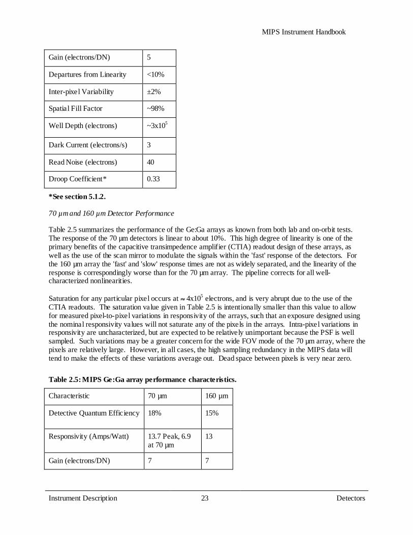
Table 2.4: MIPS Si:As BIB array performance characteristics.
Characteristic
Detective Quantum Efficiency
~ 60%
MIPS Instrument Handbook
Instrument Description 23
Detectors
Gain (electrons/DN) 5
Departures from Linearity <10%
Inter-pixel Variability ±2%
Spatial Fill Factor ~98%
Well Depth (electrons) ~3x10⁵
Dark Current (electrons/s) 3
Read Noise (electrons) 40
Droop Coefficient* 0.33
*See section 5.1.2.
70 µm and 160 µm Detector Performance
Table 2.5 summarizes the performance of the Ge:Ga arrays as known from both lab and on-orbit tests. The response of the 70 µm detectors is linear to about 10%. This high degree of linearity is one of the primary benefits of the capacitive transimpedence amplifier (CTIA) readout design of these arrays, as well as the use of the scan mirror to modulate the signals within the 'fast' response of the detectors. For the 160 µm array the 'fast' and 'slow' response times are not as widely separated, and the linearity of the response is correspondingly worse than for the 70 µm array. The pipeline corrects for all well-characterized nonlinearities. Saturation for any particular pixel occurs at 4x10⁵ electrons, and is very abrupt due to the use of the CTIA readouts. The saturation value given in Table 2.5 is intentionally smaller than this value to allow for measured pixel-to-pixel variations in responsivity of the arrays, such that an exposure designed using the nominal responsivity values will not saturate any of the pixels in the arrays. Intra-pixel variations in responsivity are uncharacterized, but are expected to be relatively unimportant because the PSF is well sampled. Such variations may be a greater concern for the wide FOV mode of the 70 µm array, where the pixels are relatively large. However, in all cases, the high sampling redundancy in the MIPS data will tend to make the effects of these variations average out. Dead space between pixels is very near zero.
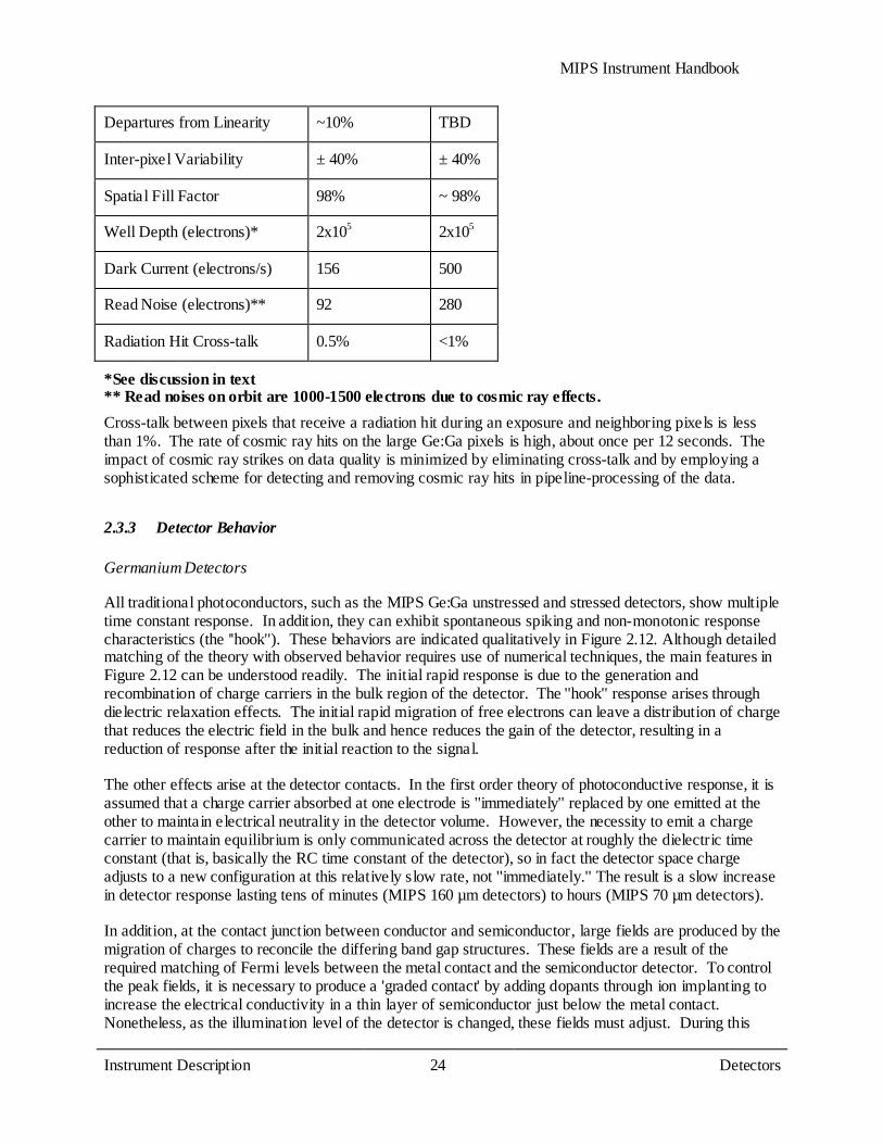
Table 2.5: MIPS Ge:Ga array performance characteristics.
Characteristic 70 µm 160 µm
Detective Quantum Efficiency 18% 15%
Responsivity (Amps/Watt) 13.7 Peak, 6.9 at 70 µm
13
Gain (electrons/DN) 7 7
MIPS Instrument Handbook
Instrument Description 24
Detectors
Departures from Linearity ~10% TBD
Inter-pixel Variability ± 40% ± 40%
Spatial Fill Factor 98% ~ 98%
Well Depth (electrons)* 2x10⁵ 2x10⁵
Dark Current (electrons/s) 156 500
Read Noise (electrons)** 92 280
Radiation Hit Cross-talk 0.5% <1%
*See discussion in text ** Read noises on orbit are 1000-1500 electrons due to cosmic ray effects. Cross-talk between pixels that receive a radiation hit during an exposure and neighboring pixels is less than 1%. The rate of cosmic ray hits on the large Ge:Ga pixels is high, about once per 12 seconds. The impact of cosmic ray strikes on data quality is minimized by eliminating cross-talk and by employing a sophisticated scheme for detecting and removing cosmic ray hits in pipeline-processing of the data.
2.3.3 Detector Behavior
Germanium Detectors
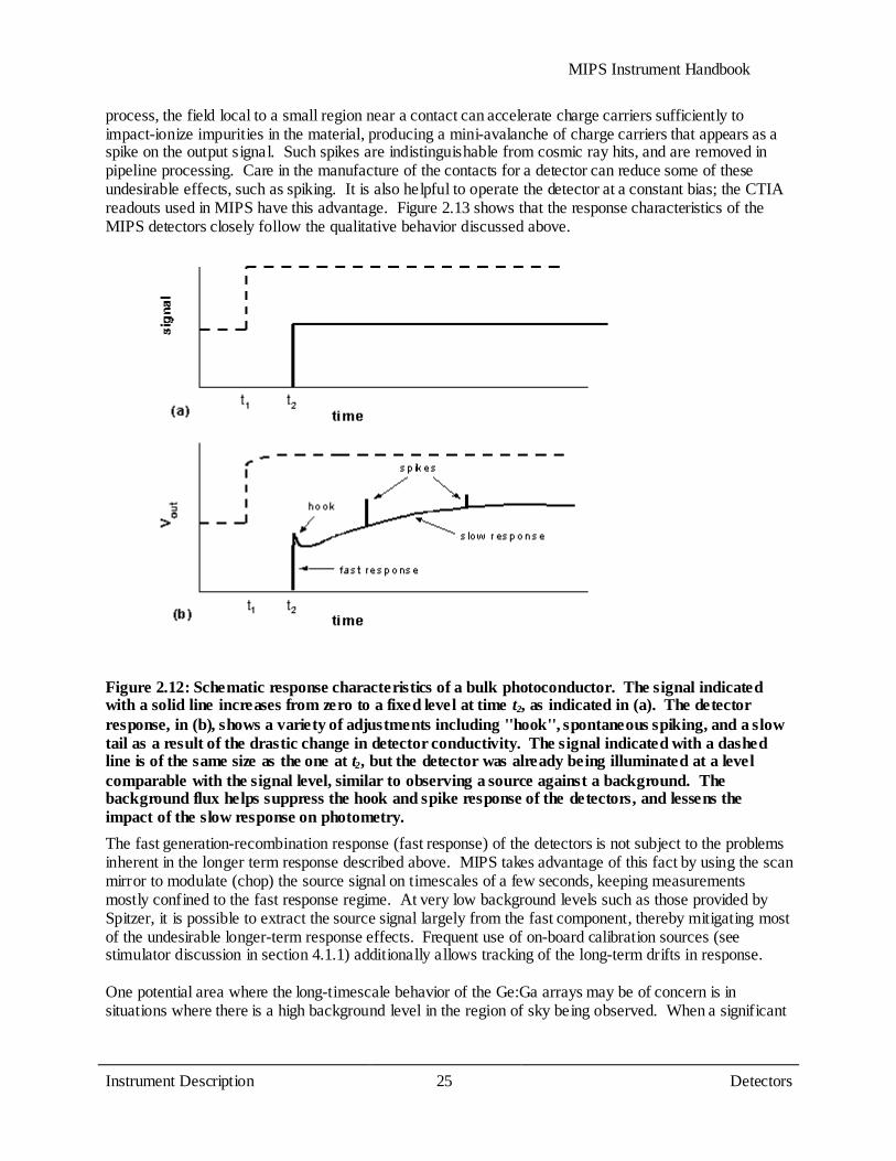
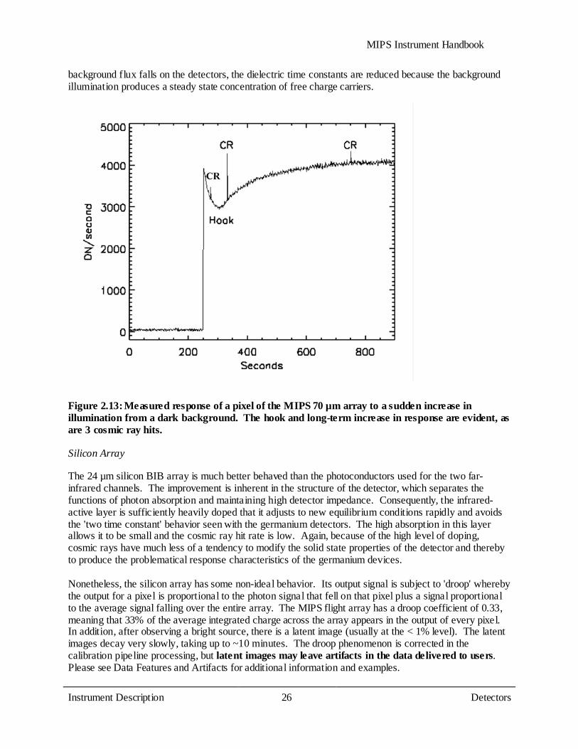
All traditional photoconductors, such as the MIPS Ge:Ga unstressed and stressed detectors, show multiple time constant response. In addition, they can exhibit spontaneous spiking and non-monotonic response characteristics (the ''hook''). These behaviors are indicated qualitatively in Figure 2.12. Although detailed matching of the theory with observed behavior requires use of numerical techniques, the main features in Figure 2.12 can be understood readily. The initial rapid response is due to the generation and recombination of charge carriers in the bulk region of the detector. The ''hook'' response arises through dielectric relaxation effects. The initial rapid migration of free electrons can leave a distribution of charge that reduces the electric field in the bulk and hence reduces the gain of the detector, resulting in a reduction of response after the initial reaction to the signal. The other effects arise at the detector contacts. In the first order theory of photoconductive response, it is assumed that a charge carrier absorbed at one electrode is ''immediately'' replaced by one emitted at the other to maintain electrical neutrality in the detector volume. However, the necessity to emit a charge carrier to maintain equilibrium is only communicated across the detector at roughly the dielectric time constant (that is, basically the RC time constant of the detector), so in fact the detector space charge adjusts to a new configuration at this relatively slow rate, not ''immediately.'' The result is a slow increase in detector response lasting tens of minutes (MIPS 160 µm detectors) to hours (MIPS 70 µm detectors). In addition, at the contact junction between conductor and semiconductor, large fields are produced by the migration of charges to reconcile the differing band gap structures. These fields are a result of the required matching of Fermi levels between the metal contact and the semiconductor detector. To control the peak fields, it is necessary to produce a 'graded contact' by adding dopants through ion implanting to increase the electrical conductivity in a thin layer of semiconductor just below the metal contact. Nonetheless, as the illumination level of the detector is changed, these fields must adjust. During this
MIPS Instrument Handbook
Instrument Description 25
Detectors
process, the field local to a small region near a contact can accelerate charge carriers sufficiently to impact-ionize impurities in the material, producing a mini-avalanche of charge carriers that appears as a spike on the output signal. Such spikes are indistinguishable from cosmic ray hits, and are removed in pipeline processing. Care in the manufacture of the contacts for a detector can reduce some of these undesirable effects, such as spiking. It is also helpful to operate the detector at a constant bias; the CTIA readouts used in MIPS have this advantage. Figure 2.13 shows that the response characteristics of the MIPS detectors closely follow the qualitative behavior discussed above.
Figure 2.12: Schematic response characteristics of a bulk photoconductor. The signal indicated with a solid line increases from zero to a fixed level at time t2, as indicated in (a). The detector response, in (b), shows a variety of adjustments including ''hook'', spontaneous spiking, and a slow tail as a result of the drastic change in detector conductivity. The signal indicated with a dashed line is of the same size as the one at t2, but the detector was already being illuminated at a level comparable with the signal level, similar to observing a source against a background. The background flux helps suppress the hook and spike response of the detectors, and lessens the impact of the slow response on photometry. The fast generation-recombination response (fast response) of the detectors is not subject to the problems inherent in the longer term response described above. MIPS takes advantage of this fact by using the scan mirror to modulate (chop) the source signal on timescales of a few seconds, keeping measurements mostly confined to the fast response regime. At very low background levels such as those provided by Spitzer, it is possible to extract the source signal largely from the fast component, thereby mitigating most of the undesirable longer-term response effects. Frequent use of on-board calibration sources (see stimulator discussion in section 4.1.1) additionally allows tracking of the long-term drifts in response. One potential area where the long-timescale behavior of the Ge:Ga arrays may be of concern is in situations where there is a high background level in the region of sky being observed. When a significant
MIPS Instrument Handbook
Instrument Description 26
Detectors
background flux falls on the detectors, the dielectric time constants are reduced because the background illumination produces a steady state concentration of free charge carriers.
Figure 2.13: Measured response of a pixel of the MIPS 70 µm array to a sudden increase in illumination from a dark background. The hook and long-term increase in response are evident, as are 3 cosmic ray hits.
Silicon Array
The 24 µm silicon BIB array is much better behaved than the photoconductors used for the two far-infrared channels. The improvement is inherent in the structure of the detector, which separates the functions of photon absorption and maintaining high detector impedance. Consequently, the infrared-active layer is sufficiently heavily doped that it adjusts to new equilibrium conditions rapidly and avoids the 'two time constant' behavior seen with the germanium detectors. The high absorption in this layer allows it to be small and the cosmic ray hit rate is low. Again, because of the high level of doping, cosmic rays have much less of a tendency to modify the solid state properties of the detector and thereby to produce the problematical response characteristics of the germanium devices. Nonetheless, the silicon array has some non-ideal behavior. Its output signal is subject to 'droop' whereby the output for a pixel is proportional to the photon signal that fell on that pixel plus a signal proportional to the average signal falling over the entire array. The MIPS flight array has a droop coefficient of 0.33, meaning that 33% of the average integrated charge across the array appears in the output of every pixel. In addition, after observing a bright source, there is a latent image (usually at the < 1% level). The latent images decay very slowly, taking up to ~10 minutes. The droop phenomenon is corrected in the calibration pipeline processing, but latent images may leave artifacts in the data delivered to users. Please see Data Features and Artifacts for additional information and examples.
MIPS Instrument Handbook
Instrument Description 27
Electronics
2.3.4 Annealing and Stimulator Use
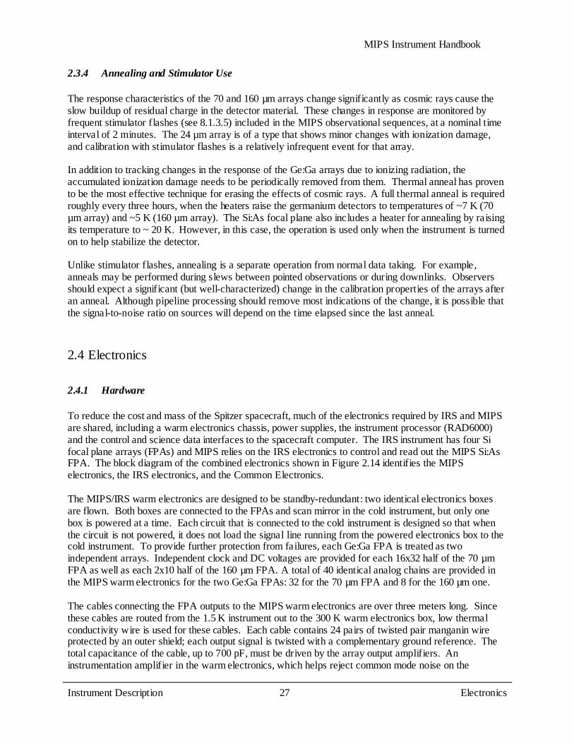
The response characteristics of the 70 and 160 µm arrays change significantly as cosmic rays cause the slow buildup of residual charge in the detector material. These changes in response are monitored by frequent stimulator flashes (see 8.1.3.5) included in the MIPS observational sequences, at a nominal time interval of 2 minutes. The 24 µm array is of a type that shows minor changes with ionization damage, and calibration with stimulator flashes is a relatively infrequent event for that array. In addition to tracking changes in the response of the Ge:Ga arrays due to ionizing radiation, the accumulated ionization damage needs to be periodically removed from them. Thermal anneal has proven to be the most effective technique for erasing the effects of cosmic rays. A full thermal anneal is required roughly every three hours, when the heaters raise the germanium detectors to temperatures of ~7 K (70 µm array) and ~5 K (160 µm array). The Si:As focal plane also includes a heater for annealing by raising its temperature to ~ 20 K. However, in this case, the operation is used only when the instrument is turned on to help stabilize the detector. Unlike stimulator flashes, annealing is a separate operation from normal data taking. For example, anneals may be performed during slews between pointed observations or during downlinks. Observers should expect a significant (but well-characterized) change in the calibration properties of the arrays after an anneal. Although pipeline processing should remove most indications of the change, it is possible that the signal-to-noise ratio on sources will depend on the time elapsed since the last anneal.
2.4 Electronics
2.4.1 Hardware
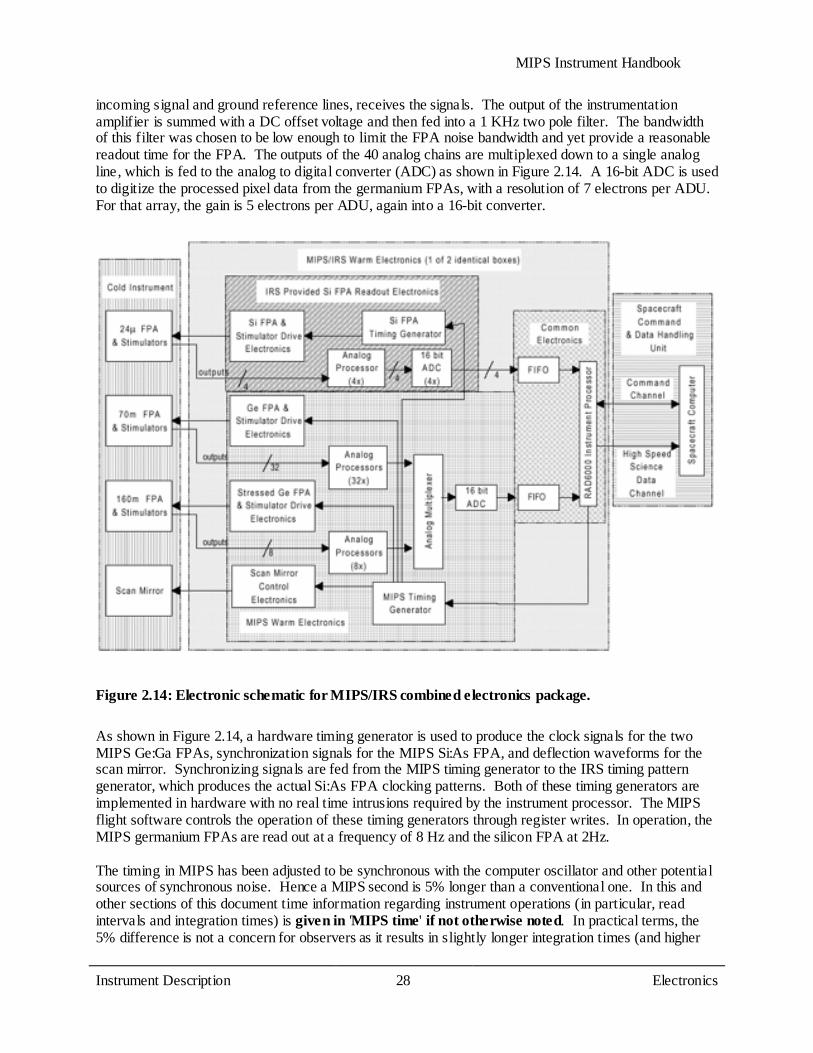
To reduce the cost and mass of the Spitzer spacecraft, much of the electronics required by IRS and MIPS are shared, including a warm electronics chassis, power supplies, the instrument processor (RAD6000) and the control and science data interfaces to the spacecraft computer. The IRS instrument has four Si focal plane arrays (FPAs) and MIPS relies on the IRS electronics to control and read out the MIPS Si:As FPA. The block diagram of the combined electronics shown in Figure 2.14 identifies the MIPS electronics, the IRS electronics, and the Common Electronics. The MIPS/IRS warm electronics are designed to be standby-redundant: two identical electronics boxes are flown. Both boxes are connected to the FPAs and scan mirror in the cold instrument, but only one box is powered at a time. Each circuit that is connected to the cold instrument is designed so that when the circuit is not powered, it does not load the signal line running from the powered electronics box to the cold instrument. To provide further protection from failures, each Ge:Ga FPA is treated as two independent arrays. Independent clock and DC voltages are provided for each 16x32 half of the 70 µm FPA as well as each 2x10 half of the 160 µm FPA. A total of 40 identical analog chains are provided in the MIPS warm electronics for the two Ge:Ga FPAs: 32 for the 70 µm FPA and 8 for the 160 µm one. The cables connecting the FPA outputs to the MIPS warm electronics are over three meters long. Since these cables are routed from the 1.5 K instrument out to the 300 K warm electronics box, low thermal conductivity wire is used for these cables. Each cable contains 24 pairs of twisted pair manganin wire protected by an outer shield; each output signal is twisted with a complementary ground reference. The total capacitance of the cable, up to 700 pF, must be driven by the array output amplifiers. An instrumentation amplifier in the warm electronics, which helps reject common mode noise on the
MIPS Instrument Handbook
Instrument Description 28
Electronics
incoming signal and ground reference lines, receives the signals. The output of the instrumentation amplifier is summed with a DC offset voltage and then fed into a 1 KHz two pole filter. The bandwidth of this filter was chosen to be low enough to limit the FPA noise bandwidth and yet provide a reasonable readout time for the FPA. The outputs of the 40 analog chains are multiplexed down to a single analog line, which is fed to the analog to digital converter (ADC) as shown in Figure 2.14. A 16-bit ADC is used to digitize the processed pixel data from the germanium FPAs, with a resolution of 7 electrons per ADU. For that array, the gain is 5 electrons per ADU, again into a 16-bit converter.
Figure 2.14: Electronic schematic for MIPS/IRS combined electronics package. As shown in Figure 2.14, a hardware timing generator is used to produce the clock signals for the two MIPS Ge:Ga FPAs, synchronization signals for the MIPS Si:As FPA, and deflection waveforms for the scan mirror. Synchronizing signals are fed from the MIPS timing generator to the IRS timing pattern generator, which produces the actual Si:As FPA clocking patterns. Both of these timing generators are implemented in hardware with no real time intrusions required by the instrument processor. The MIPS flight software controls the operation of these timing generators through register writes. In operation, the MIPS germanium FPAs are read out at a frequency of 8 Hz and the silicon FPA at 2Hz. The timing in MIPS has been adjusted to be synchronous with the computer oscillator and other potential sources of synchronous noise. Hence a MIPS second is 5% longer than a conventional one. In this and other sections of this document time information regarding instrument operations (in particular, read intervals and integration times) is given in 'MIPS time' if not otherwise noted. In practical terms, the 5% difference is not a concern for observers as it results in slightly longer integration times (and higher
MIPS Instrument Handbook
Instrument Description 29
Electronics
sensitivity) than would nominally be achieved. See section 3.4.1 for specific information regarding the impact on sensitivity and integration time estimates. Times returned by the archive are in real seconds , and transparently account for the 5% timing stretch within the MIPS hardware. Drivers are provided in the MIPS electronics for the FPA calibration stimulator sources and the thermal anneal heaters. The timing generator produces the stimulator flash pulses, which are synchronized with the FPA readout. The thermal anneal heater timing is controlled directly by the instrument processor. The CSMM (scan mirror) is controlled by a type I analog servo system. The actual CSMM deflection angle is continuously monitored and compared with the commanded angle. The error signal between the actual and desired positions is integrated and used to drive the CSMM actuator. Mirror deflection commands are generated digitally by the timing generator and converted to an analog command using a digital-to-analog converter (DAC). The timing generator produces all the required CSMM deflection waveforms, including chop waveforms and the sawtooth pattern required by the MIPS scan map mode. The higher currents required by the CSMM and by the FPA thermal anneal heaters are carried to the cold instrument over a cable constructed of phosphor bronze wire.
2.4.2 Software
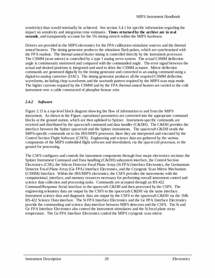
Figure 2.15 is a top-level block diagram showing the flow of information to and from the MIPS instrument. As shown in the Figure, operational parameters are converted into the appropriate command blocks at the ground station, which are then uplinked to Spitzer. Instrument-specific commands are received and distributed by the spacecraft command and data handler (C&DH). The C&DH provides the interface between the Spitzer spacecraft and the Spitzer instruments. The spacecraft C&DH sends the MIPS-specific commands on to the IRS/MIPS processor; there they are interpreted and executed by the Control Section Flight Software (CSFS). Engineering and science data are gathered by the various components of the MIPS embedded flight software and downlinked, via the spacecraft processor, to the ground for processing. The CSFS configures and controls the instrument components through four major electronics sections: the Spitzer Instrument Command and Data handling (C&DH) subsystem interface, the Control Section Electronics (CSE), the Silicon Detector Focal Plane Array (Si FPA) Interface Electronics, the Germanium Detector Focal Plane Array (Ge FPA) Interface Electronics, and the Cryogenic Scan Mirror Mechanism (CSMM) Interface. Within the IRS/MIPS electronics, the CSFS provides the instruments with the computational, interface, and memory resources necessary for performing overall instrument control and science data collection and processing tasks. Commands are accepted through an RS-422 Command/Response Serial interface to the spacecraft C&DH and then processed by the CSFS. The engineering telemetry data are output by the CSFS to the spacecraft C&DH via the same interface. Instrument science data and diagnostic data are output by the CSFS to the spacecraft C&DH via the 1Mb RS-422 Science Data interface. The Si FPA Interface Electronics and the Ge FPA Interface Electronics provide the commanding and science data interface between MIPS detectors and the CSFS. The Si and Ge FPA Interface Electronics also control the instrument stimulators and the Si focal plane array temperature. The Ge FPA Interface Electronics control the MIPS cryogenic scan mirror.
MIPS Instrument Handbook
Instrument Description 30
Electronics
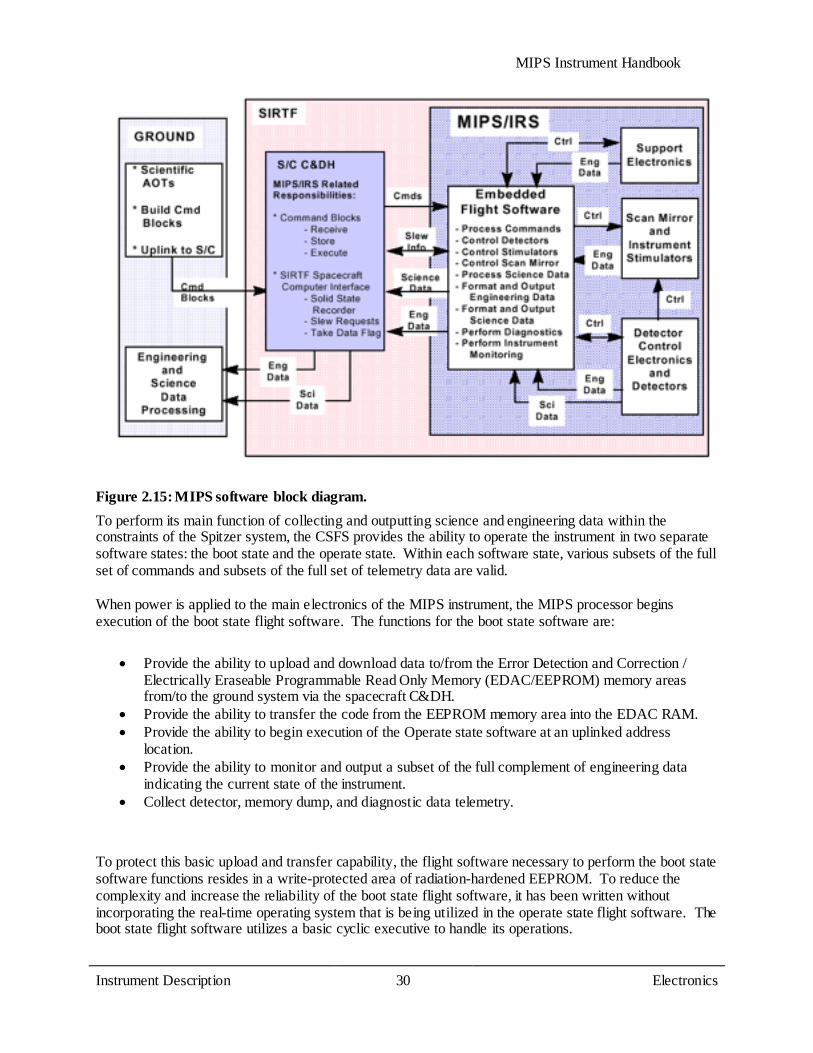
Figure 2.15: MIPS software block diagram. To perform its main function of collecting and outputting science and engineering data within the constraints of the Spitzer system, the CSFS provides the ability to operate the instrument in two separate software states: the boot state and the operate state. Within each software state, various subsets of the full set of commands and subsets of the full set of telemetry data are valid. When power is applied to the main electronics of the MIPS instrument, the MIPS processor begins execution of the boot state flight software. The functions for the boot state software are:
• Provide the ability to upload and download data to/from the Error Detection and Correction / Electrically Eraseable Programmable Read Only Memory (EDAC/EEPROM) memory areas from/to the ground system via the spacecraft C&DH.
• Provide the ability to transfer the code from the EEPROM memory area into the EDAC RAM. • Provide the ability to begin execution of the Operate state software at an uplinked address
location. • Provide the ability to monitor and output a subset of the full complement of engineering data
indicating the current state of the instrument. • Collect detector, memory dump, and diagnostic data telemetry.
To protect this basic upload and transfer capability, the flight software necessary to perform the boot state software functions resides in a write-protected area of radiation-hardened EEPROM. To reduce the complexity and increase the reliability of the boot state flight software, it has been written without incorporating the real-time operating system that is being utilized in the operate state flight software. The boot state flight software utilizes a basic cyclic executive to handle its operations.

MIPS Instrument Handbook
Instrument Description 31
Electronics
After the boot state software has copied the operate state software from EEPROM to EDAC RAM, the instrument may be commanded into the operate state, where instrument science activities can be performed. All instrument calibrations, science observations and instrument diagnostic activities are performed by the operate state software. To accomplish this, the operate state software supports the following tasks:
• Configure and operate the MIPS detectors. • Configure and operate the MIPS scan mirror. • Configure and control the MIPS instrument stimulators. • Collect detector, memory dump, and diagnostic data telemetry. • Collect and monitor engineering data and scan mirror position data. • Format and output science data to the RS-422 Serial interface. • Format and output engineering telemetry data to the RS-422 Serial interface.
2.4.3 Array Control
So far as possible within the constraints of data compression and telemetry limitations, each image in the Ge:Ga and stressed Ge:Ga bands is sent to the ground for further processing, which removes cosmic ray hits and other bad data, shifts and adds the frames, and calibrates them to produce the final images of the sky. The Si:As data are fitted onboard by linear regression for each pixel and only the slopes for each image are sent to the ground (along with a difference of the first two reads). This processing is required to limit the amount of data that must be stored by the spacecraft.
32x32 Ge:Ga Array (70 µm)
The 32x32 array readouts consist of CTIA amplifiers which are ''on'' continuously, and whose outputs are sampled sequentially by an on-chip multiplexer. The MUX is cycled at a constant rate to give a read rate of 8 samples per pixel per MIPS second. Each sample is digitized and stored on the spacecraft using lossless compression. The preservation of the detailed data stream for each pixel is critical for this (and the 160 µm) array because of the large hit rate by ionizing particles, as much as 1 hit per pixel per 35 seconds. These hits can only be removed from the data stream in ground processing. The array is reset coincident with a scan mirror flyback, and then reset again half a second later to commence gathering data.
2x20 Stressed Ge:Ga Array (160 µm)
Operations are similar to the 32x32 array. One distinct difference between operations of the two arrays is that when the observer requests a 10 sec exposure, the 160 µm exposure is split into two 5 sec exposures by resetting the array half-way through the full exposure time. Because of the generally high level of background flux at 160 µm, the array saturates too quickly to be useful in many portions of the sky if a 10 sec exposure is used. An added benefit of performing an extra reset of the 160 µm array is superior rejection of cosmic-ray hits. The extra reset is entirely internal to the MIPS commanding software and instrument, and is transparent to observers.
128x128 Si:As BIB Array (24 µm)
The 128x128 array also takes data in a mode similar to that just described for the 32x32 array, but some minor differences are required because of differences in its readout, its larger format, and its differing
MIPS Instrument Handbook
Instrument Description 32
Sensitivity
susceptibility to hits by ionizing particles. The array is read out at a constant rate, every 0.5 MIPS sec, and the resulting data sent to the IRS/MIPS computer for processing. However, the data rate is too high to allow sending every frame to the ground. Fortunately, because it has smaller pixels than the 32x32 array (by more than 1000 in surface area), the cosmic ray hit rate is much smaller and it is permissible to process the frames from the multiple reads into a single image (the net integration between resets) before sending it to the ground. The net signal for each pixel in an image is computed by linear regression to determine the current generated by the pixel between resets. However, there is a loss in dynamic range in this process, since a source that saturates a pixel during the integration will be unrecoverable. To achieve the dynamic range requirements for MIPS, it is necessary also to retrieve the information from the initial 0.5 MIPS sec integration. To do so, the first and second reads of the array are differenced and also sent to the ground. The readout and resetting of this array proceeds continuously over 0.5 sec, recycling to the same state for the next 0.5 sec. Therefore, the final set of reads for a given integration must start 0.5 sec before the scan mirror flyback. Following reading the array, each pixel is reset during the 0.5 sec read cycle while the scan mirror flies back. A second 0.5 sec reset cycle follows to remove residual signals accumulated during flyback before the scan mirror has settled. Integration on each pixel begins immediately after this second reset. That is, for every scan mirror flyback, there is a one second dead time for each pixel of the Si:As array, and these deadtimes are distributed over a 0.5 sec offset in the order of pixel access and read, with the first pixels beginning integration 0.5 sec after flyback is initiated and the last ones 1 sec after flyback initiation.
2.5 Sensitivity
The performance of MIPS in actual use depends on many factors. The performance of the arrays themselves is important, but telescope and optical throughput also play an important role. An important factor for users to consider when predicting the sensitivity of a given measurement is the sky background present in the field of interest. Sources of background flux vary with wavelength and position on the sky. The character of the far-infrared background as understood at the time of observation is described below.
2.5.1 Imaging: Sources of Noise and Confusion
At 70 µm, zodiacal light (thermal emission from warm dust within the Solar System) and Galactic cirrus (thermal emission from warm dust clouds in the Galaxy) dominate the background. Zodiacal light is smooth on the scale of a MIPS frame, and decreases by roughly a factor of 4 between sight-lines near the ecliptic plane and towards the ecliptic pole. Zodiacal emission at a particular RA and Dec also varies as a function of time due to the orbital motions of both Spitzer and the zodiacal dust. As a rule-of-thumb, the zodiacal emission can be expected to change by about 1% over a one-day period. Galactic cirrus is concentrated near the Galactic plane, and varies on many spatial scales, including scales that are not resolved by MIPS. Structures within the cirrus include wisps and small knots, and are thus of interest, not only because of the background flux they contribute, but also because they can potentially be confused with sources of interest. The level of cirrus varies greatly, and must be evaluated in detail for observations where high sensitivity at 70 µm is desired. Galactic cirrus contributes somewhat to the confusing structure of the background, but especially at long wavelengths, this structure is dominated by emission from partially-resolved and unresolved distant galaxies. Observations that are subject to this background are frequently referred to as ''confusion

MIPS Instrument Handbook
Instrument Description 33
Sensitivity
limited,'' because the spatial structure resembles the superposition of many point sources, and determining whether a particular faint source is a part of the background or is a target can be difficult. The structure of the background effectively increases its noise contribution above what would be calculated based on the flux contributed by all of the sources in a region. The structure contributes directly to the variance of the background as it would be measured by aperture or PSF-fitting photometry extraction software, for example. The accuracy of photometry at 70 and 160 µm will often be confusion-limited. Because MIPS provides much smaller effective beams and higher sensitivity than any previous mission, predicting the confusion limit set by such sources is difficult. Pre-launch estimates of the 1σ confusion limits ranged from about 0.5 to 1.3 mJy at 70 µm, and from about 7 to 19 mJy at 160 µm (Xu et al. 2001, ApJ, 562, 179; Franceschini et al., 2002, ESO conference proceedings, astro-ph/0202463; and Dole et al. 2003, ApJ, 585, 617). Mission data from MIPS produced the following source density criterion (SDC) limits for confusion, due to extragalactic sources (Dole et al. 2004, ApJS, 154, 93): 56 µJy at 24 µm, 3.2 mJy at 70 µm, and 40 mJy at 160 µm. The 5σ photometric confusion limit at 70 µm is 1.5 mJy (Frayer et al. 2006, ApJ, 647, L9). At 24 and 70 µm, the confusion mainly results from the high density of resolved sources; at 160 µm, the confusion arises from a population fainter than the sensitivity limit; see Dole et al. (2004, ApJS, 154, 93). There is a range of values expected, and moreover it can be a function of where exactly one looks in the sky. Note that confusion due to Galactic sources is a strong function of position. Other factors may influence the effective confusion limit for a particular observation. In some instances it may have been reasonable to integrate somewhat below the level of the confusion, for example when the observer had a priori knowledge of a source position. On the other hand, the presence of a nearby bright source with its diffraction artifacts will increase the effective confusion limit. Moving targets offer the possibility of taking a second ''shadow'' observation, allowing the suppression of confusing sources by subtracting them away. Observers were also warned that they needed to specify AORs with enough cycles to provide adequate rejection of cosmic rays and other artifacts, even if a very short integration would nominally be adequate to reach the confusion limit.
2.5.2 Estimating Background
During the Spitzer mission background noise estimation tools could be done using Spot, the Spitzer Observation Planning Tool. An estimation of the background and the contribution of the various components to the background (e.g., zodiacal light) could be obtained from the target selection window. While the noise levels predicted via Spot were based on previous infrared space observations at lower sensitivity and spatial resolution than MIPS obtains, they were the best products available at the time for making such estimates. The Spot model did reasonably well (see, e.g., Dole et al., 2004, ApJS, 154, 93 and Meadows et al., 2004, ApJS, 154, 469). The only exception to this is in regions where the infrared cirrus levels are low. In these low-cirrus regions it is preferable to use a cirrus estimate based on the atomic hydrogen column density in the direction of the target. The hydrogen column density is highly correlated with the cirrus background in regions where the cirrus background is well measured. This correlation can be extrapolated to provide an estimate of low-cirrus regions. However one estimates backgrounds, the aperture size used to estimate background is important. If you need help estimating backgrounds and can not find a relevant tool on our website, please contact the Helpdesk for further information.
MIPS Instrument Handbook
Instrument Description 34
Sensitivity
2.5.3 Estimating Signal-To-Noise Ratio and Integration Time
In nearly all observing circumstances, MIPS will be background-limited. That is, the dominant source of noise in the final measurement of the brightness of an object is noise contributed by emission from the background rather than the noise due to the photon statistics of the flux from the object itself. In the background-limited case, the signal-to-noise (S/N) ratio of an observation increases linearly with the flux from the object, and it increases as the square root of the integration time:
(2.2)
Where the subscript ''0'' refers to values obtained from the sensitivity plots (discussed below and on the Spitzer Heritage website), and the subscript ''obj'' refers to the desired object. F is the energy or photon flux from the object per second, I is the integration time in seconds, and B is the background surface brightness. (See next section for sensitivity information.) While this equation suggests that arbitrarily high signal-to-noise can be achieved by taking long enough integrations, in practice the signal-to-noise that can be attained is finite. The details of the confusion noise sources discussed above set a lower limit on both the fluxes that can be detected, and a corresponding upper limit on the signal-to-noise ratio that can be obtained for sources of low to moderate brightness. The S/N that can be achieved on bright sources is limited by the reproducibility of measurements taken with the MIPS arrays (see section 4.1.3). The reproducibility within a set of measurements is roughly 1% in relative flux; the repeatability from one set of measurements to another (e.g., photometry repeated on a source) is 8-10% rms. Observers are reminded that timing patterns within MIPS result in ''seconds'' which are 5% longer than a real second.
2.5.4 Sensitivity vs. Exposure Time
Although we have just emphasized that the sensitivity of MIPS depends strongly on where one is looking on the sky, we have included here the results in the best sky regions. Note that starting in 2005, regular MIPS operations changed to include ''cold'' (telescope at ~5.5 K) and ''warm'' (telescope at ~8.5 K) campaigns. The sensitivity at 24 and 70 µm remains the same for any MIPS campaign; the 160 µm array is completely saturated during MIPS-warm campaigns, so its sensitivity is not relevant. The sensitivity of the 24 µm band is shown in Figure 2.16 and Figure 2.17. The detector array is well behaved and the values for S/N can be scaled as the inverse square root of the integration time for point and extended sources. The analogous plots for the other bands are available on the website. The conversion of point source sensitivity to extended source sensitivity can be found in Table 2.6. Because of the multiple response times of the far infrared arrays, sensitivity estimation is more complex for them. The best values require high-pass filtering to remove the slow component of response; see Chapter 7: Data Features and Artifacts for additional information (including practical advice) on such filtering. The high-pass filtering also suppresses extended emission from sources. Good data can be obtained on such sources, but it requires careful hand processing to remove ''streaks'' left from slow response effects. Such removal can best be done on scan map data, and it is highly desirable to obtain scans over the source in both directions.
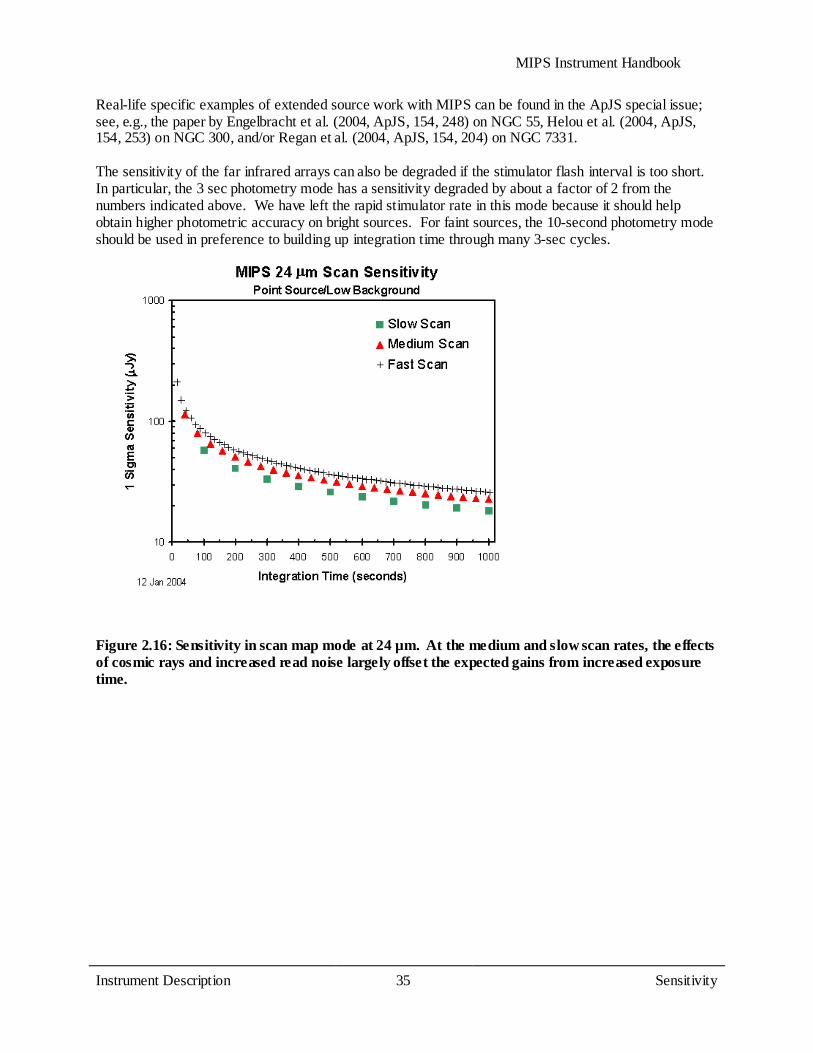
MIPS Instrument Handbook
Instrument Description 35
Sensitivity
Real-life specific examples of extended source work with MIPS can be found in the ApJS special issue; see, e.g., the paper by Engelbracht et al. (2004, ApJS, 154, 248) on NGC 55, Helou et al. (2004, ApJS, 154, 253) on NGC 300, and/or Regan et al. (2004, ApJS, 154, 204) on NGC 7331. The sensitivity of the far infrared arrays can also be degraded if the stimulator flash interval is too short. In particular, the 3 sec photometry mode has a sensitivity degraded by about a factor of 2 from the numbers indicated above. We have left the rapid stimulator rate in this mode because it should help obtain higher photometric accuracy on bright sources. For faint sources, the 10-second photometry mode should be used in preference to building up integration time through many 3-sec cycles.
Figure 2.16: Sensitivity in scan map mode at 24 µm. At the medium and slow scan rates, the effects of cosmic rays and increased read noise largely offset the expected gains from increased exposure time.
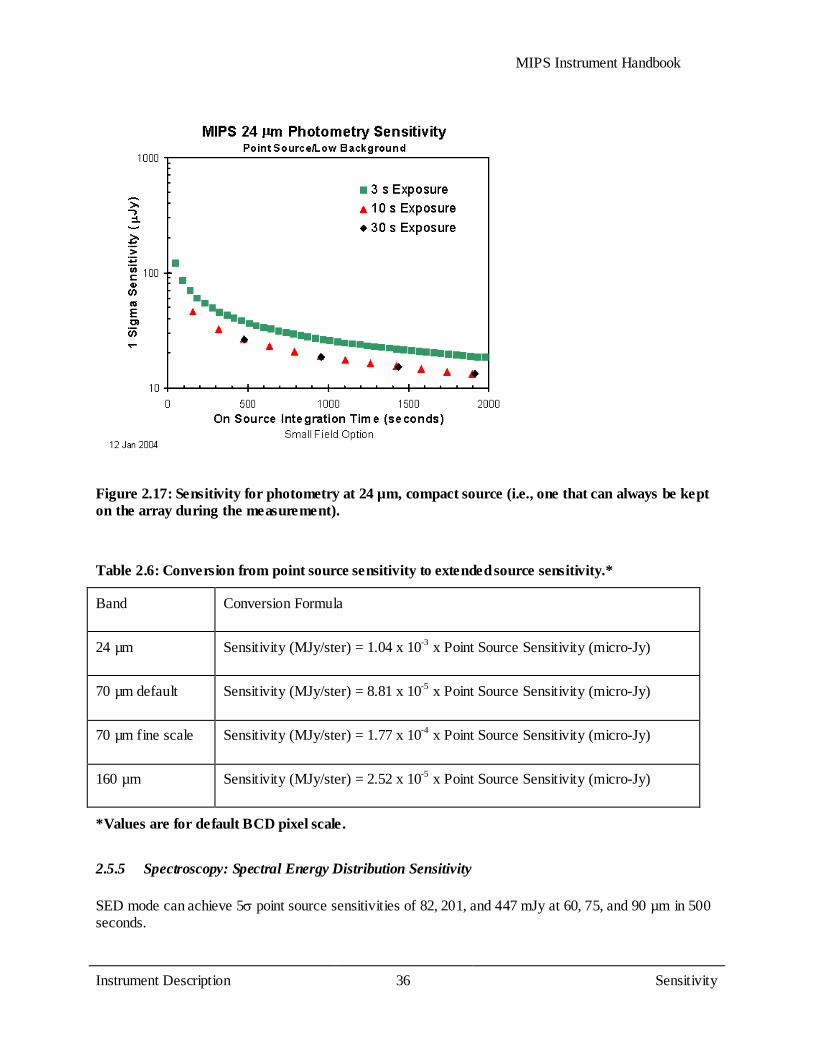
MIPS Instrument Handbook
Instrument Description 36
Sensitivity
Figure 2.17: Sensitivity for photometry at 24 µm, compact source (i.e., one that can always be kept on the array during the measurement).
Table 2.6: Conversion from point source sensitivity to extended source sensitivity.*
Band Conversion Formula
24 µm Sensitivity (MJy/ster) = 1.04 x 10⁻³ x Point Source Sensitivity (micro-Jy)
70 µm default Sensitivity (MJy/ster) = 8.81 x 10⁻⁵ x Point Source Sensitivity (micro-Jy)
70 µm fine scale Sensitivity (MJy/ster) = 1.77 x 10⁻⁴ x Point Source Sensitivity (micro-Jy)
160 µm Sensitivity (MJy/ster) = 2.52 x 10⁻⁵ x Point Source Sensitivity (micro-Jy)
*Values are for default BCD pixel scale.
2.5.5 Spectroscopy: Spectral Energy Distribution Sensitivity
SED mode can achieve 5σ point source sensitivities of 82, 201, and 447 mJy at 60, 75, and 90 µm in 500 seconds.
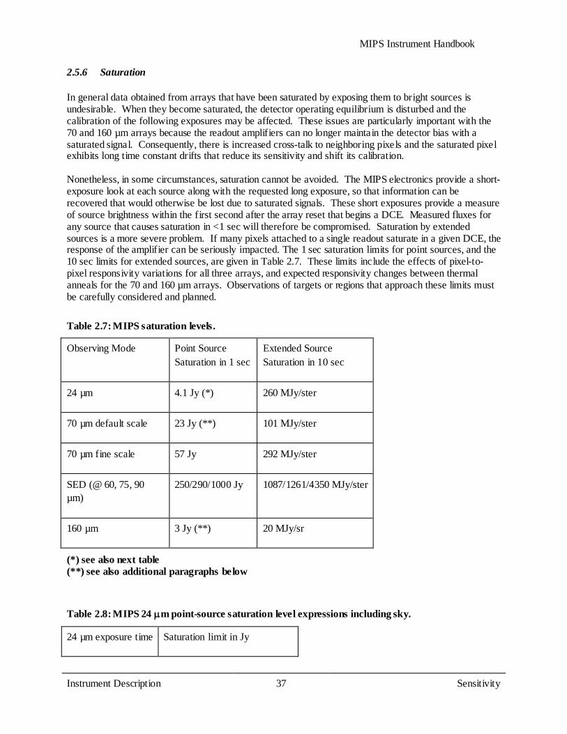
MIPS Instrument Handbook
Instrument Description 37
Sensitivity
2.5.6 Saturation
In general data obtained from arrays that have been saturated by exposing them to bright sources is undesirable. When they become saturated, the detector operating equilibrium is disturbed and the calibration of the following exposures may be affected. These issues are particularly important with the 70 and 160 µm arrays because the readout amplifiers can no longer maintain the detector bias with a saturated signal. Consequently, there is increased cross-talk to neighboring pixels and the saturated pixel exhibits long time constant drifts that reduce its sensitivity and shift its calibration. Nonetheless, in some circumstances, saturation cannot be avoided. The MIPS electronics provide a short-exposure look at each source along with the requested long exposure, so that information can be recovered that would otherwise be lost due to saturated signals. These short exposures provide a measure of source brightness within the first second after the array reset that begins a DCE. Measured fluxes for any source that causes saturation in <1 sec will therefore be compromised. Saturation by extended sources is a more severe problem. If many pixels attached to a single readout saturate in a given DCE, the response of the amplifier can be seriously impacted. The 1 sec saturation limits for point sources, and the 10 sec limits for extended sources, are given in Table 2.7. These limits include the effects of pixel-to-pixel responsivity variations for all three arrays, and expected responsivity changes between thermal anneals for the 70 and 160 µm arrays. Observations of targets or regions that approach these limits must be carefully considered and planned.
Table 2.7: MIPS saturation levels.
Observing Mode Point Source Saturation in 1 sec
Extended Source Saturation in 10 sec
24 µm 4.1 Jy (*) 260 MJy/ster
70 µm default scale 23 Jy (**) 101 MJy/ster
70 µm fine scale 57 Jy 292 MJy/ster
SED (@ 60, 75, 90 µm)
250/290/1000 Jy 1087/1261/4350 MJy/ster
160 µm 3 Jy (**) 20 MJy/sr
(*) see also next table (**) see also additional paragraphs below
Table 2.8: MIPS 24 µm point-source saturation level expressions including sky.
24 µm exposure time Saturation limit in Jy

MIPS Instrument Handbook
Instrument Description 38
Sensitivity
3 sec 1.64 - 8.0x10⁻⁴ x(sky in MJy/sr)
4 sec 1.17 - 5.7x10⁻⁴ x(sky in MJy/sr)
10 sec 0.43 - 2.1x10⁻⁴ x(sky in MJy/sr)
30 sec 0.14 - 6.8x10⁻⁵ x(sky in MJy/sr)
The general case for observations involves a combination of extended and point-like emission. The implications of saturation for the 24 µm array can be computed by assuming a combination of the effects in Table 2.7, as seen in Table 2.8. For example, if the estimated background at 24 µm is 100 MJy/ster, it uses up 40% of the dynamic range in a 10 second integration. Without the background, a source of 0.5 Jy would not saturate in a 10 second integration. However, only 60% of the dynamic range is left on top of the background, so the brightest measurable source in a 10 second integration is 0.4 Jy (from the 10-sec formula in Table 2.8). Many users attempt to derive Table 2.7 from Table 2.8. We would like to point out that this is not possible. The values for truly ideal cases are in Table 2.7. The formulae in Table 2.8 actually describe the general case, which includes a combination of point and background flux, so they break down in the limiting cases. Further complicating matters, Table 2.8 also has incorporated into it subframes that are part of the observing sequence AND the impact of some substitution of values for point sources - there is a half-second data frame taken at the beginning of the observing sequence, and we can use the first difference to substitute in values for point sources that are saturated later in the exposure. The values in Table 2.7 are meant to be single-point values, with nothing hidden. The values in Table 2.8 are a better approximation to reality: a mixture of point and background sources, subframes that are part of the observing sequence, and the use of some of these subframes to substitute saturated pixels. For extended source 24 µm saturation limits, the 10-second limit from Table 2.7 (260 MJy/sr) can be scaled by a factor of 9.5 /(exposure time - 0.5). At 70 µm, some targets slightly brighter than these limits can be usefully observed. However, the consequences for the immediately following reads are significant, with latent images and a degradation of linearity. If known about beforehand, an attempt was made to schedule such observations near a thermal anneal, but this was not always the case. Note that, since our calibrators are not this bright, observations of objects this bright may not be as well-calibrated as fainter objects. At 160 µm, the saturation limit for a 3 second integration is about 1 Jy. For sources brighter than this level, up to about 4 Jy, useful data will be obtained on the first few reads, but the brightest pixels will saturate before the end of the integration. As a result, there will be some degradation of the results in the readouts immediately following, but the recovery will be relatively fast. Note that there is no equivalent to Table 2.8 for 70 and 160 µm; the equivalent effects (ramp fitting to just the points before saturation) are already included in the values given in Table 2.7 above.
Several programs had observations with severely compromised signal-to-noise ratios because the observers chose long exposure times (30 sec) in regions where the background due to zodiacal light was very high. In these cases, the slope image becomes saturated during the exposure and a large fraction of

MIPS Instrument Handbook
Instrument Description 39
Sensitivity
the array had the ''soft'' saturated 30 sec slope image replaced with pixels from the unsaturated, but much noisier, difference image (see section 5.1.2). The difference image represents only about 0.5 sec of exposure time. Thus, the use of the 30 sec exposure time has instead resulted in BCD images dominated by only 0.5 sec of exposure time! Better designed programs to detect faint sources superposed on high backgrounds made use of coadding many shorter exposures (for photometry mode, 3 or 10 sec exposures).
A simple calculation using the numbers from Table 2.8 indicates that the extended 24 µm saturation limit for a 30 sec exposure should be 84 MJy/sr. We note that this is the hard saturation level at which even the difference image will be saturated. The approximate soft saturation limits are given in Table 2.9.
Table 2.9: MIPS 24 µm soft saturation levels.
24 µm exposure time
Saturation level in MJy/sr
30 sec 60
10 sec 180
3 sec 600

MIPS Instrument Handbook
Operating Modes 40
Sensitivity
Chapter 3 Operating Modes
There are four major operational modes (or Astronomical Observation Templates; AOTs) of the MIPS instrument:
• Scan Map (includes slow, medium and fast scan rates, where incomplete coverage at 160 µm is obtained at the fast scan rate).
• Photometry and Super Resolution (PH/SR; includes super-resolution, large source, and small source options, and can be used to obtain multiple images through the cluster and raster-map options).
• Spectral Energy Distribution (SED; can be used for a single spectrum or step and stare spectral mapping).
• Total Power Mode (TP; used to obtain absolute brightness measurements for highly extended sources).
Observing in any of these modes involved the acquisition of multiple data frames, not just a single frame. The multiplicity of frames provides for rejection of cosmic rays, calibration of the Ge:Ga focal plane array data in the light of the two-time-constant behavior of those detectors, adequate sampling of the point spread function (PSF; especially for super resolution observations), and, in the case of the 160 µm array, for building up a filled image using multiple offset exposures of that 2x20 pixel array. The total number of images obtained depends on the total integration time needed, the observational mode, and the array. For all AOTs, the number of cycles is the number of times the basic observing sequence or full map sequence was executed, as described below. Observers are reminded that in photometry/super-resolution mode, MIPS always took multiple, dithered frames, each with the specified exposure time. Because of this, the total exposure time is an integer multiple of the single frame exposure time and the number of dither positions imposed on all photometry AORs; the total on-source integration time is quantized as a result. The number of cycles selection determines how many of these integration-time quanta will be obtained. Likewise, on-source integration time is quantized in scan-map mode, depending on the selected scan rate, and selecting more than one scan cycle will build up integration time in multiples of that single-cycle integration time. Observers could specify that a small region (a raster map) be covered in photometry mode. The entire AOT cycle is repeated at each raster map location; the number of map cycles is different and refers to the number of times the whole map is repeated. Because of noise improvements relating to characteristics of the stressed Ge:Ga 160 µm detectors, when a 10 sec exposure time is selected, the 160 µm detectors were reset twice within the exposure interval. This effectively resulted in two exposures at 160 µm before dithering when using the 10 sec exposure option. The 160 µm sensitivities for 10 sec exposures include the multiple resets. The Cluster Option was a way to conveniently specify repetitions of one or multiple observations at several closely grouped pointings (within approximately 1° of initial target). The observations done at each cluster position are identical, and done in the same pointing sequences as for a single target AOR. The observational modes that can be specified under the cluster option are MIPS Photometry/Super Resolution, SED, and TP. Also, observations of moving targets could be made in a co-moving frame for all MIPS AOTs, including Scan Map.

MIPS Instrument Handbook
Operating Modes 41
Photometry Mode
3.1 Photometry Mode
Although both photometry and super resolution were supported in a single AOT, for illustration we describe the procedures separately. The photometry mode was designed to obtain multi-band observations of reasonably compact sources; sources that are too extended for the procedures described below should generally have been imaged using MIPS scan mapping (section 3.2) instead. Super resolution emphasizes robust sampling of the point spread function through a combination of small pixels relative to the Airy disk and of sub-stepping of the image relative to the pixels. Special observing modes were used to achieve this goal at 70 and 160 µm, and at 70 µm a separate optical train providing a finer pixel scale was also employed. Note that super-resolution data requires additional post-processing (beyond what the Spitzer pipeline provides) to extract higher spatial resolution. In the following descriptions, we give overly specific examples with particular pixel addresses for where the image falls. We do so for purposes of illustration only. Actual placements on the arrays may not be exactly those given here, but relative placement remains. Observers are referred to Table 3.4 below for a summary of photometry mode integration times. Note also that the multiplicity of frames is prescribed within the AOTs, and the observer selected the number of times (cycles) to repeat the basic pattern of a template in order to build up the desired integration time. There are multiple options within the photometry AOT. ''Compact source'' can also be referred to as ''small field, '' and ''large source'' as ''large field. '' Additionally, for 70 µm, ''fine scale'' pixels can also occasionally be referred to as ''narrow field, '' and ''default scale'' can be described as ''coarse scale. ''
3.1.1 Photometry - 24 µm, Compact Source (Small Field)
One cycle of the basic 24 µm photometry observation acquires 14 separate images of a source. The locations of these 14 images are illustrated in Figure 3.1 and listed in Table 3.1. To start the observation sequence, the source is centered to the left of the array center by 25 pixels (65´ )́ and the scanning mirror is chopped in a nearly symmetrical fashion, above and below the array center, to obtain a column of 7 images. The spacecraft is then slewed to position the source 25.5 pixels (66.3´ )́ to the right of center and another column of 7 images is obtained. Table 3.1 contains the resulting approximate image positions in units of pixels, with the origin taken to be the center of the array. Array distortion and the twist of the scanning mirror with respect to the array columns have not been taken into account in this table, but the positions are good enough for observation planning purposes. The observer specifies only one parameter, the number of observing cycles. If the observer specifies N cycles, the sequence repeats the first column N times before the spacecraft moves to take N sets of data in the second column. There are two complications to this simple scenario: (1) two extra exposures are obtained at positions 1 and 8 for each AOR, and (2) exposures 1 and 8 of the first cycle (and a few subsequent cycles in long AORs) are one second shorter than the specified exposure time. Spot takes this all into account when it calculates the total integration time, but it is approximately ((Nx14)+2) x (Exposure Time)-2 seconds. The 2 sec reduction comes about because the first second of frames 1 and 8 are used for obtaining calibration data, not science data.

MIPS Instrument Handbook
Operating Modes 42
Photometry Mode
Figure 3.1: Photometry/Super Resolution for compact sources with the 24 µm array. The positions of images in a single cycle of a 24 µm photometry observation are shown relative to the central 64x64 pixels (shown schematically by the grid) of the full 128x128 array. The circle diameters are the FWHM of the Airy disk. The first set of 7 images are dithered using the scan mirror, then the spacecraft is offset by a half-integer number of pixels, and the second 7 images are acquired. Frames 1 and 8 of the first cycle of an AOR (and a few subsequent cycles in long AORs) are 1 sec shorter than the observer-requested exposure time; the other 12 frames of such cycles are taken with the full observer-specified exposure time. Not shown are 2 additional frames, taken at the positions 1 and 8, obtained for each AOR. Note that half of the images are obtained at each spacecraft pointing. The telescope relative offset accuracy allows meaningful fractional pixel offsets. Moreover, in practice, alignment tolerances make the chop motion slightly non-parallel to the array columns. In any case, the implemented pattern provides a well-sampled Airy disk. Although for simple photometry, the images can be combined by integer shifts, careful processing will be required to take full advantage of the oversampling implicit in these images.
Table 3.1: Source positions for 24 µm compact source photometry (in units of pixels, the origin being the center of the array).
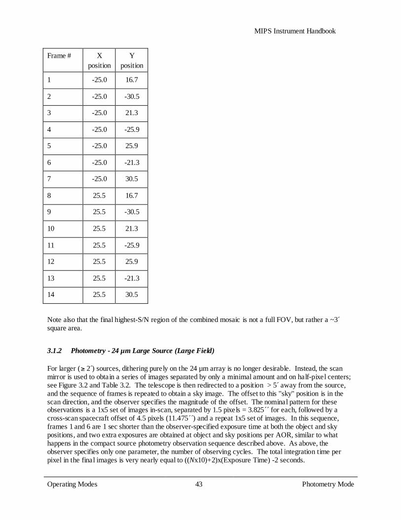
MIPS Instrument Handbook
Operating Modes 43
Photometry Mode
Frame # X position
Y position
1 -25.0 16.7
2 -25.0 -30.5
3 -25.0 21.3
4 -25.0 -25.9
5 -25.0 25.9
6 -25.0 -21.3
7 -25.0 30.5
8 25.5 16.7
9 25.5 -30.5
10 25.5 21.3
11 25.5 -25.9
12 25.5 25.9
13 25.5 -21.3
14 25.5 30.5
Note also that the final highest-S/N region of the combined mosaic is not a full FOV, but rather a ~3 ́square area.
3.1.2 Photometry - 24 µm Large Source (Large Field)
For larger ( 2 )́ sources, dithering purely on the 24 µm array is no longer desirable. Instead, the scan mirror is used to obtain a series of images separated by only a minimal amount and on half-pixel centers; see Figure 3.2 and Table 3.2. The telescope is then redirected to a position > 5 ́away from the source, and the sequence of frames is repeated to obtain a sky image. The offset to this ''sky'' position is in the scan direction, and the observer specifies the magnitude of the offset. The nominal pattern for these observations is a 1x5 set of images in-scan, separated by 1.5 pixels = 3.825´ ́for each, followed by a cross-scan spacecraft offset of 4.5 pixels (11.475´ )́ and a repeat 1x5 set of images. In this sequence, frames 1 and 6 are 1 sec shorter than the observer-specified exposure time at both the object and sky positions, and two extra exposures are obtained at object and sky positions per AOR, similar to what happens in the compact source photometry observation sequence described above. As above, the observer specifies only one parameter, the number of observing cycles. The total integration time per pixel in the final images is very nearly equal to ((Nx10)+2)x(Exposure Time) -2 seconds.
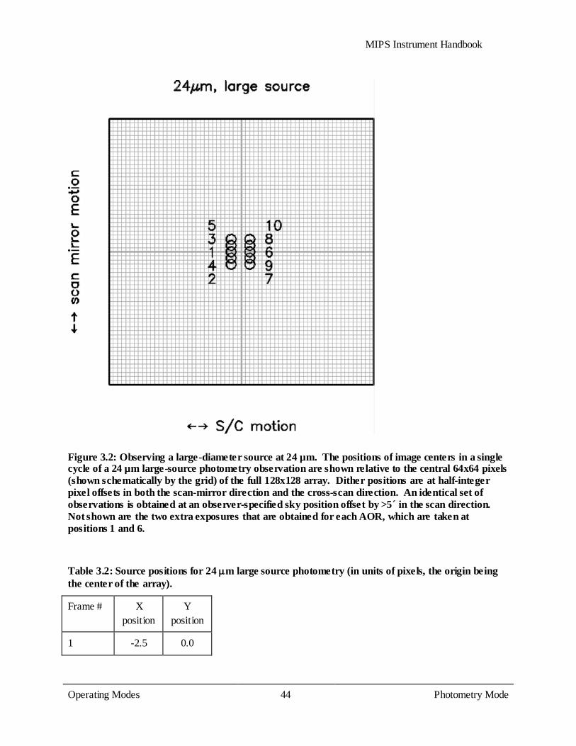
MIPS Instrument Handbook
Operating Modes 44
Photometry Mode
Figure 3.2: Observing a large-diameter source at 24 µm. The positions of image centers in a single cycle of a 24 µm large-source photometry observation are shown relative to the central 64x64 pixels (shown schematically by the grid) of the full 128x128 array. Dither positions are at half-integer pixel offsets in both the scan-mirror direction and the cross-scan direction. An identical set of observations is obtained at an observer-specified sky position offset by >5´ in the scan direction. Not shown are the two extra exposures that are obtained for each AOR, which are taken at positions 1 and 6.
Table 3.2: Source positions for 24 µm large source photometry (in units of pixels, the origin being the center of the array).
Frame # X position
Y position
1 -2.5 0.0

MIPS Instrument Handbook
Operating Modes 45
Photometry Mode
2 -2.5 -3.1
3 -2.5 1.5
4 -2.5 -1.6
5 -2.5 3.1
6 2.0 0.0
7 2.0 -3.1
8 2.0 1.5
9 2.0 -1.6
10 2.0 3.1
As before, Table 3.2 contains the resulting approximate image positions in units of pixels, with the origin taken to be the center of the array. Array distortion and the twist of the scanning mirror with respect to the array columns have not been taken into account in this table, but the positions are good enough for observation planning purposes.
3.1.3 Photometry - 70 µm Compact Source (Small Field), Default Pixel Scale
Typical photometry observations at 70 µm are made using the nominal 9.8´ ́pixel scale. The super-resolution mode at 70 µm also provides excellent data for photometry, but is considerably more expensive in terms of observing time overhead and is also about 4 times less sensitive. In the normal photometry observation of a compact (< 1 )́ target (see Figure 3.3), a pattern of observations is made that is similar in concept to the 24 µm compact source photometry observation. As a result of the on-orbit realities, we made changes to our pre-launch plans for this mode; it resembles the pre-launch AOT, but shifted to the less noisy side (side A) and with the amplitudes of the offsets correspondingly scaled down in the cross-scan direction. To start the observation sequence, the source is centered to the left of the array center by 9 pixels (98´ )́, 1 pixel to the left of the center of side A (the good side), and the scanning mirror is chopped in a symmetrical fashion, above and below the array center to obtain a column of 6 images — the first and last are both at the central position. The spacecraft is then slewed to position the source 7.5 pixels to the left of center (74´ )́, 0.5 pixel to the right of the center of side A, and another column of images is obtained. The resulting approximate image positions are given in Table 3.3, where the coordinates are in pixels and the origin is taken to be the center of the array. Array distortion and twist have not been taken into account in this table. In reality, the images will not fall exactly on the positions given in this table, but these positions are good enough for observation planning purposes.
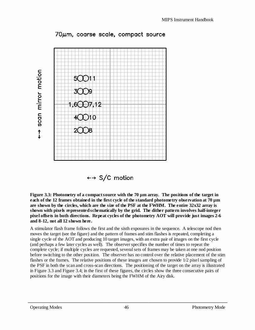
MIPS Instrument Handbook
Operating Modes 46
Photometry Mode
Figure 3.3: Photometry of a compact source with the 70 µm array. The positions of the target in each of the 12 frames obtained in the first cycle of the standard photometry observation at 70 µm are shown by the circles, which are the size of the PSF at the FWHM. The entire 32x32 array is shown with pixels represented schematically by the grid. The dither pattern involves half-integer pixel offsets in both directions. Repeat cycles of the photometry AOT will provide just images 2-6 and 8-12, not all 12 shown here. A stimulator flash frame follows the first and the sixth exposures in the sequence. A telescope nod then moves the target (see the figure) and the pattern of frames and stim flashes is repeated, completing a single cycle of the AOT and producing 10 target images, with an extra pair of images on the first cycle (and perhaps a few later cycles as well). The observer specifies the number of times to repeat the complete cycle; if multiple cycles are requested, several sets of frames may be taken at one nod position before switching to the other position. The observer has no control over the relative placement of the stim flashes or the frames. The relative positions of these images are chosen to provide 1/2 pixel sampling of the PSF in both the scan and cross-scan directions. The positioning of the target on the array is illustrated in Figure 3.3 and Figure 3.4; in the first of these figures, the circles show the three consecutive pairs of positions for the image with their diameters being the FWHM of the Airy disk.
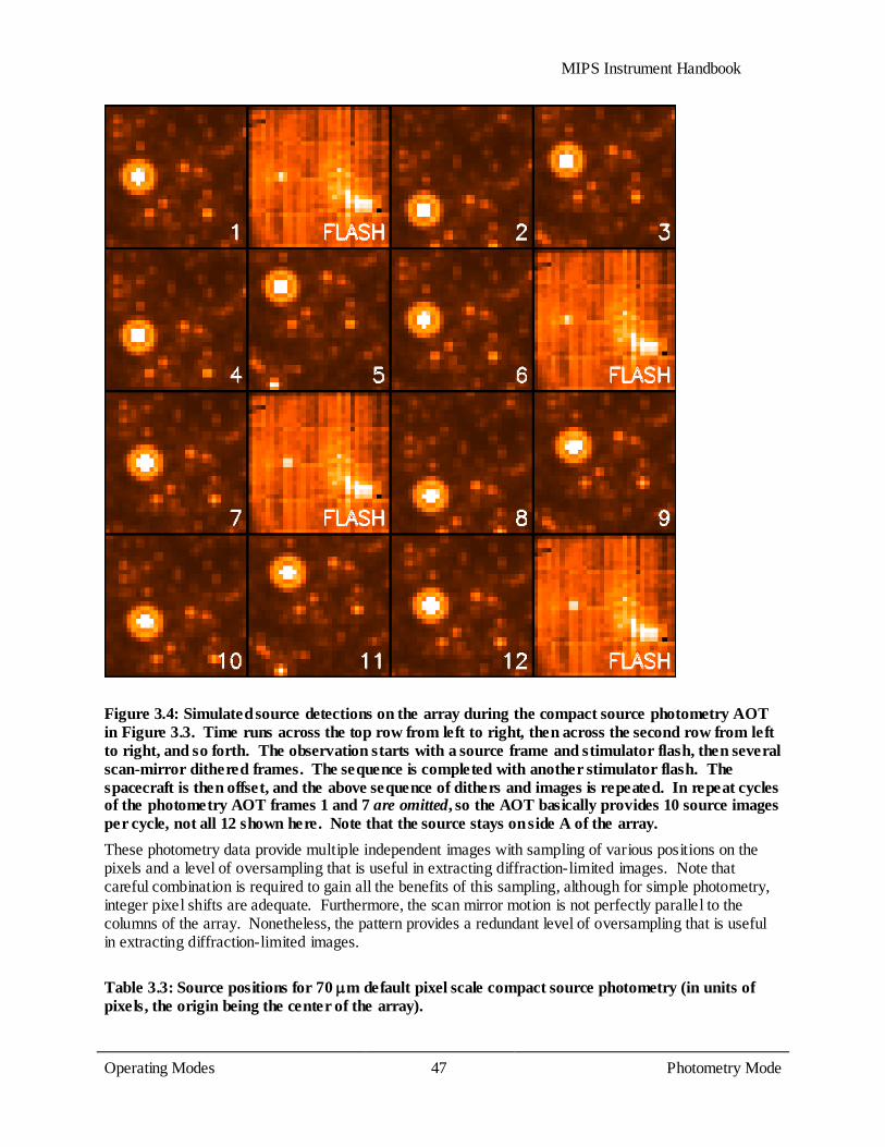
MIPS Instrument Handbook
Operating Modes 47
Photometry Mode
Figure 3.4: Simulated source detections on the array during the compact source photometry AOT in Figure 3.3. Time runs across the top row from left to right, then across the second row from left to right, and so forth. The observation starts with a source frame and stimulator flash, then several scan-mirror dithered frames. The sequence is completed with another stimulator flash. The spacecraft is then offset, and the above sequence of dithers and images is repeated. In repeat cycles of the photometry AOT frames 1 and 7 are omitted, so the AOT basically provides 10 source images per cycle, not all 12 shown here. Note that the source stays on side A of the array. These photometry data provide multiple independent images with sampling of various positions on the pixels and a level of oversampling that is useful in extracting diffraction-limited images. Note that careful combination is required to gain all the benefits of this sampling, although for simple photometry, integer pixel shifts are adequate. Furthermore, the scan mirror motion is not perfectly parallel to the columns of the array. Nonetheless, the pattern provides a redundant level of oversampling that is useful in extracting diffraction-limited images.
Table 3.3: Source positions for 70 µm default pixel scale compact source photometry (in units of pixels, the origin being the center of the array).
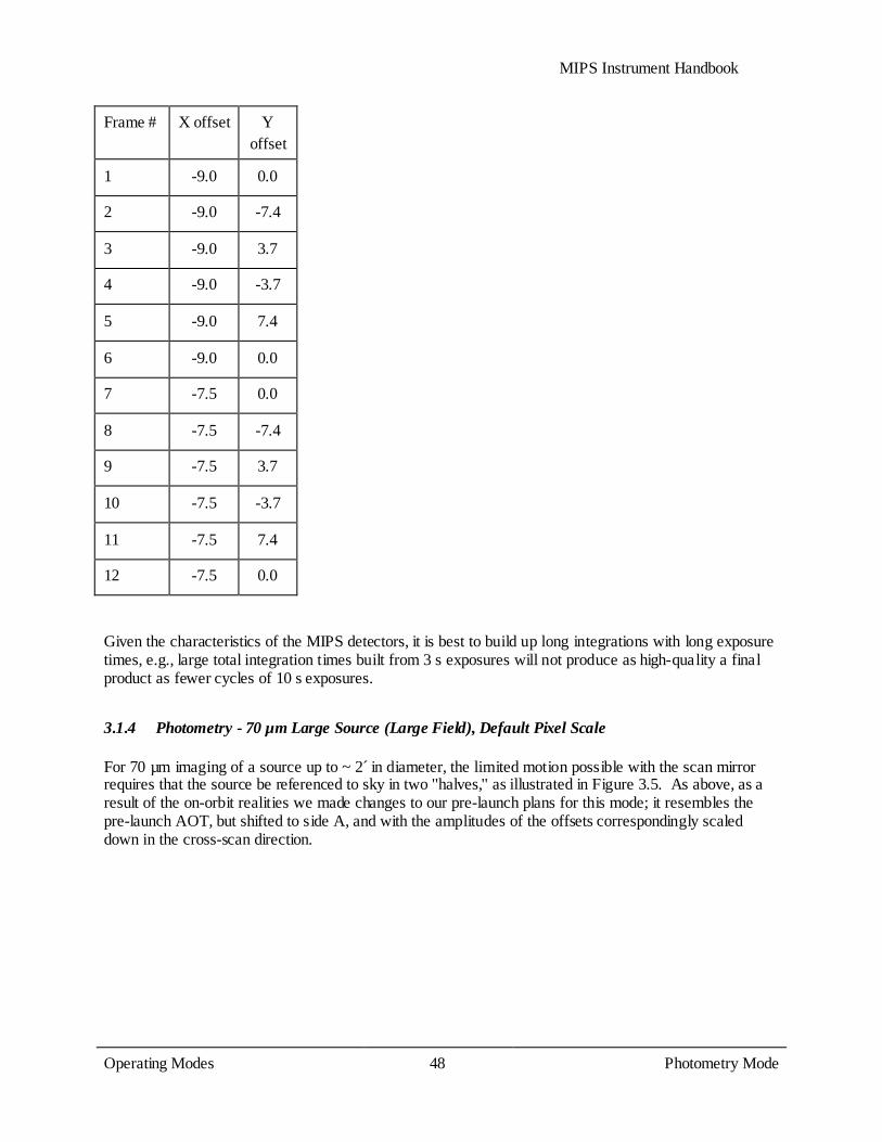
MIPS Instrument Handbook
Operating Modes 48
Photometry Mode
Frame # X offset Y offset
1 -9.0 0.0
2 -9.0 -7.4
3 -9.0 3.7
4 -9.0 -3.7
5 -9.0 7.4
6 -9.0 0.0
7 -7.5 0.0
8 -7.5 -7.4
9 -7.5 3.7
10 -7.5 -3.7
11 -7.5 7.4
12 -7.5 0.0
Given the characteristics of the MIPS detectors, it is best to build up long integrations with long exposure times, e.g., large total integration times built from 3 s exposures will not produce as high-quality a final product as fewer cycles of 10 s exposures.
3.1.4 Photometry - 70 µm Large Source (Large Field), Default Pixel Scale
For 70 µm imaging of a source up to ~ 2 ́in diameter, the limited motion possible with the scan mirror requires that the source be referenced to sky in two ''halves,'' as illustrated in Figure 3.5. As above, as a result of the on-orbit realities we made changes to our pre-launch plans for this mode; it resembles the pre-launch AOT, but shifted to side A, and with the amplitudes of the offsets correspondingly scaled down in the cross-scan direction.

MIPS Instrument Handbook
Operating Modes 49
Photometry Mode
Figure 3.5: Photometry of a large source at 70 µm. The source is observed such that the coordinates are placed near the array center in the pattern shown. Spacecraft and scan mirror motions are made in such a way that the sky background is observed in two halves on both sides of the image in the in-scan direction. Note that for simplicity, the array is portrayed as a square; in-orbit realities mean that only half of the array is functional, and the pattern as portrayed here is centered on side A. The scan mirror starts near one end of its travel within the large-scale 70 µm range, and the spacecraft is pointed to place the source 2.5 pixels below the center of the array and 0.5 pixel to one side of the center of side A. The scan mirror is set to have a throw of 2 ,́ and the first pair of exposures is taken at the starting point (target image) and 2 ́away in-scan (sky image). A second target - sky pair is obtained with the scan mirror advanced 2.5 pixels (24.6´ )́, and a third pair obtained after advancing another 2.5 pixels. Next, the spacecraft is maneuvered 1.25 pixels in cross-scan and 2 ́in-scan, and the scan mirror is then used to obtain another three pairs of exposures, starting with a sky image, then chopping back to get the target. The overall sky coverage is illustrated in Figure 3.6.

MIPS Instrument Handbook
Operating Modes 50
Photometry Mode
Figure 3.6: Simulated source detections on the array during the large source photometry AOT shown in Figure 3.5. Time runs across the top row from left to right, then across the second row from left to right, and so forth. The observations start with an image in the sky position, then a stimulator flash, then the first source image. Three on source-off source pairs of images are taken, then a final stimulator flash. The spacecraft is then offset, there is a stimulator flash, three more on-off image pairs are taken, and the cycle is completed with a final stimulator flash. In repeat cycles of the AOT, frames 1 and 7 are omitted, so the AOT basically provides 6 source-sky image pairs per cycle. Note that the source stays on side A of the array. Note that the viable part of the array is a 2.5´x5 ́rectangle, but since the orientation of the field of view on the sky is a function of time and generally observers could not specify the time of their observation, the largest object that should have been observed using this mode is <2 .́ Because of the smaller effective size of the 70 µm array compared to previous expectations, some users needed to efficiently map the approximately 5´x5 ́(2.5´x2.5 ́fine scale) area covered by the original large-field AOT. In order to do this, we suggested that the user create a cluster target with offsets of (0, +80´ )́, (0, -80´ )́ in array coordinates observing ''offsets only.'' This allowed recovery of the full area of the original AOT while saving the slew tax from mapping with 2 AORs.
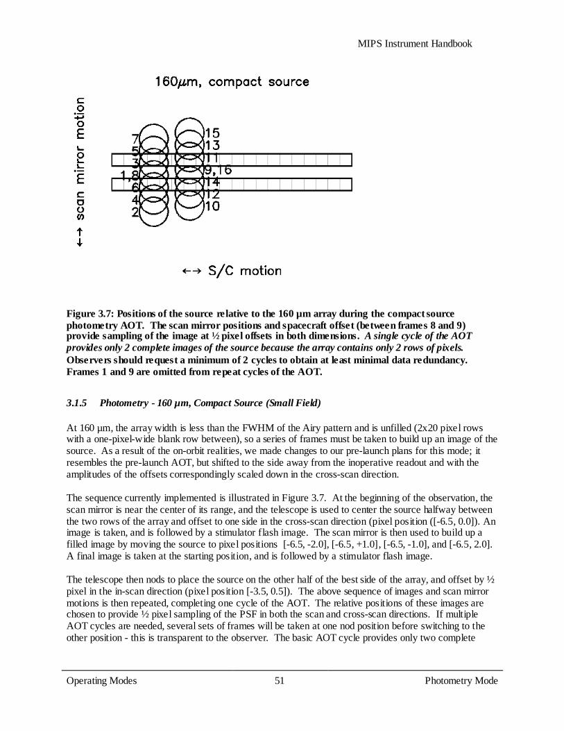
MIPS Instrument Handbook
Operating Modes 51
Photometry Mode
Figure 3.7: Positions of the source relative to the 160 µm array during the compact source photometry AOT. The scan mirror positions and spacecraft offset (between frames 8 and 9) provide sampling of the image at ½ pixel offsets in both dimensions. A single cycle of the AOT provides only 2 complete images of the source because the array contains only 2 rows of pixels. Observers should request a minimum of 2 cycles to obtain at least minimal data redundancy. Frames 1 and 9 are omitted from repeat cycles of the AOT.
3.1.5 Photometry - 160 µm, Compact Source (Small Field)
At 160 µm, the array width is less than the FWHM of the Airy pattern and is unfilled (2x20 pixel rows with a one-pixel-wide blank row between), so a series of frames must be taken to build up an image of the source. As a result of the on-orbit realities, we made changes to our pre-launch plans for this mode; it resembles the pre-launch AOT, but shifted to the side away from the inoperative readout and with the amplitudes of the offsets correspondingly scaled down in the cross-scan direction. The sequence currently implemented is illustrated in Figure 3.7. At the beginning of the observation, the scan mirror is near the center of its range, and the telescope is used to center the source halfway between the two rows of the array and offset to one side in the cross-scan direction (pixel position ([-6.5, 0.0]). An image is taken, and is followed by a stimulator flash image. The scan mirror is then used to build up a filled image by moving the source to pixel positions [-6.5, -2.0], [-6.5, +1.0], [-6.5, -1.0], and [-6.5, 2.0]. A final image is taken at the starting position, and is followed by a stimulator flash image. The telescope then nods to place the source on the other half of the best side of the array, and offset by ½ pixel in the in-scan direction (pixel position [-3.5, 0.5]). The above sequence of images and scan mirror motions is then repeated, completing one cycle of the AOT. The relative positions of these images are chosen to provide ½ pixel sampling of the PSF in both the scan and cross-scan directions. If multiple AOT cycles are needed, several sets of frames will be taken at one nod position before switching to the other position - this is transparent to the observer. The basic AOT cycle provides only two complete

MIPS Instrument Handbook
Operating Modes 52
Photometry Mode
images of the target when all dither positions are mosaicked together, with an extra pair of sub-images on the first (and perhaps a few later) cycles.
Figure 3.8: Simulated visualization of individual frames in the first cycle of the 160 µm small source photometry AOT shown in Figure 3.7 (upper panels), and a full mosaic of those frames (lower panel) with the 2 source images coadded. Note that pixels in the lower panel are shown twice as large as they are in the upper panels. Numbering along the sides shows the positions of the rows of the array during the execution of the AOT. Note that the source is offset in the final mosaic as a result of the AOT modifications to accommodate the dead readout (not shown). It was strongly recommended that observers specify at least two cycles of the 160 µm small field photometry AOT (i.e., 4 complete images) in order to provide the minimum level of redundancy. Observers were also encouraged to use the new enhanced mode (see below) which became available in Cycle 4, particularly for point source photometry. Figure 3.8 illustrates the individual pointings for a complete cycle, and a coadded mosaic (with the two individual images coadded in the central region of the mosaic). As can be seen in the figure, the AOT provides in the end an image of the target that is offset, i.e., more of the background sky is observed on one side of the target than the other.
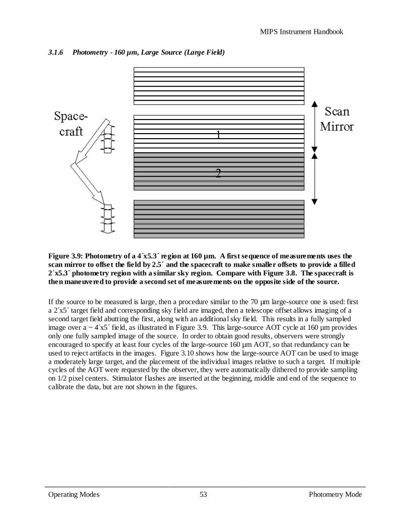
MIPS Instrument Handbook
Operating Modes 53
Photometry Mode
3.1.6 Photometry - 160 µm, Large Source (Large Field)
Figure 3.9: Photometry of a 4´x5.3 ́region at 160 µm. A first sequence of measurements uses the scan mirror to offset the field by 2.5´ and the spacecraft to make smaller offsets to provide a filled 2´x5.3 ́photometry region with a similar sky region. Compare with Figure 3.8. The spacecraft is then maneuvered to provide a second set of measurements on the opposite side of the source. If the source to be measured is large, then a procedure similar to the 70 µm large-source one is used: first a 2´x5 ́target field and corresponding sky field are imaged, then a telescope offset allows imaging of a second target field abutting the first, along with an additional sky field. This results in a fully sampled image over a ~ 4´x5 ́field, as illustrated in Figure 3.9. This large-source AOT cycle at 160 µm provides only one fully sampled image of the source. In order to obtain good results, observers were strongly encouraged to specify at least four cycles of the large-source 160 µm AOT, so that redundancy can be used to reject artifacts in the images. Figure 3.10 shows how the large-source AOT can be used to image a moderately large target, and the placement of the individual images relative to such a target. If multiple cycles of the AOT were requested by the observer, they were automatically dithered to provide sampling on 1/2 pixel centers. Stimulator flashes are inserted at the beginning, middle and end of the sequence to calibrate the data, but are not shown in the figures.
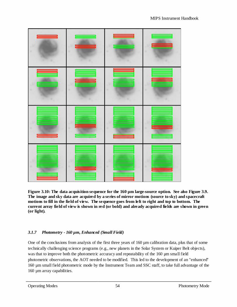
MIPS Instrument Handbook
Operating Modes 54
Photometry Mode
Figure 3.10: The data acquisition sequence for the 160 µm large-source option. See also Figure 3.9. The image and sky data are acquired by a series of mirror motions (source to sky) and spacecraft motions to fill in the field of view. The sequence goes from left to right and top to bottom. The current array field of view is shown in red (or bold) and already acquired fields are shown in green (or light).
3.1.7 Photometry - 160 µm, Enhanced (Small Field)
One of the conclusions from analysis of the first three years of 160 µm calibration data, plus that of some technically challenging science programs (e.g., new planets in the Solar System or Kuiper Belt objects), was that to improve both the photometric accuracy and repeatability of the 160 µm small field photometric observations, the AOT needed to be modified. This led to the development of an ''enhanced'' 160 µm small field photometric mode by the Instrument Team and SSC staff, to take full advantage of the 160 µm array capabilities.
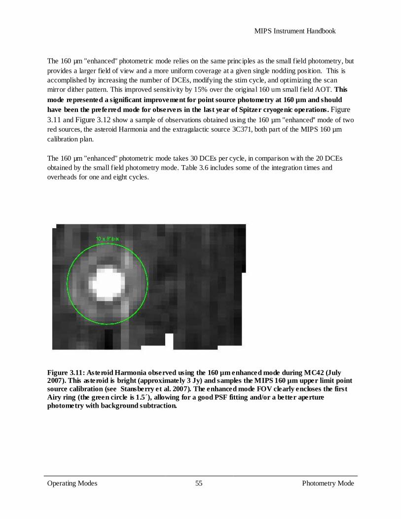
MIPS Instrument Handbook
Operating Modes 55
Photometry Mode
The 160 µm ''enhanced'' photometric mode relies on the same principles as the small field photometry, but provides a larger field of view and a more uniform coverage at a given single nodding position. This is accomplished by increasing the number of DCEs, modifying the stim cycle, and optimizing the scan mirror dither pattern. This improved sensitivity by 15% over the original 160 um small field AOT. This mode represented a significant improvement for point source photometry at 160 µm and should have been the preferred mode for observers in the last year of Spitzer cryogenic operations. Figure 3.11 and Figure 3.12 show a sample of observations obtained using the 160 µm ''enhanced'' mode of two red sources, the asteroid Harmonia and the extragalactic source 3C371, both part of the MIPS 160 µm calibration plan. The 160 µm ''enhanced'' photometric mode takes 30 DCEs per cycle, in comparison with the 20 DCEs obtained by the small field photometry mode. Table 3.6 includes some of the integration times and overheads for one and eight cycles.
Figure 3.11: Asteroid Harmonia observed using the 160 µm enhanced mode during MC42 (July 2007). This asteroid is bright (approximately 3 Jy) and samples the MIPS 160 µm upper limit point source calibration (see Stansberry et al. 2007). The enhanced mode FOV clearly encloses the first Airy ring (the green circle is 1.5´), allowing for a good PSF fitting and/or a better aperture photometry with background subtraction.
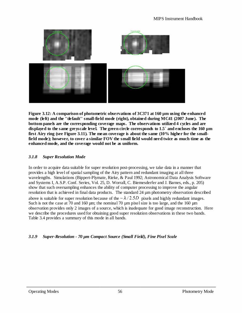
MIPS Instrument Handbook
Operating Modes 56
Photometry Mode
Figure 3.12: A comparison of photometric observations of 3C371 at 160 µm using the enhanced mode (left) and the ''default'' small-field mode (right), obtained during MC41 (2007 June). The bottom panels are the corresponding coverage maps. The observations utilized 4 cycles and are displayed to the same greyscale level. The green circle corresponds to 1.5´ and encloses the 160 µm first Airy ring (see Figure 3.11). The mean coverage is about the same (10% higher for the small-field mode); however, to cover a similar FOV the small field would need twice as much time as the enhanced mode, and the coverage would not be as uniform.
3.1.8 Super Resolution Mode
In order to acquire data suitable for super resolution post-processing, we take data in a manner that provides a high level of spatial sampling of the Airy pattern and redundant imaging at all three wavelengths. Simulations (Bippert-Plymate, Rieke, & Paul 1992; Astronomical Data Analysis Software and Systems I, A.S.P. Conf. Series, Vol. 25, D. Worrall, C. Biemesderfer and J. Barnes, eds., p. 205) show that such oversampling enhances the ability of computer processing to improve the angular resolution that is achieved in final data products. The standard 24 µm photometry observation described above is suitable for super resolution because of the ~ pixels and highly redundant images. Such is not the case at 70 and 160 µm; the nominal 70 µm pixel size is too large, and the 160 µm observation provides only 2 images of a source, which is inadequate for good image reconstruction. Here we describe the procedures used for obtaining good super resolution observations in these two bands. Table 3.4 provides a summary of this mode in all bands.
3.1.9 Super-Resolution - 70 µm Compact Source (Small Field), Fine Pixel Scale
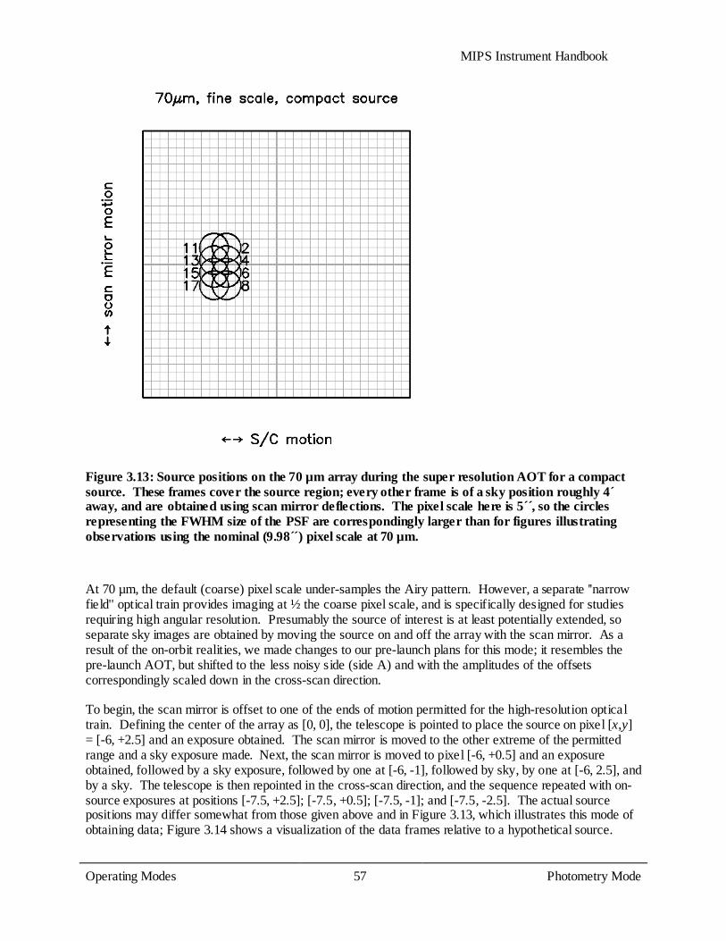
MIPS Instrument Handbook
Operating Modes 57
Photometry Mode
Figure 3.13: Source positions on the 70 µm array during the super resolution AOT for a compact source. These frames cover the source region; every other frame is of a sky position roughly 4 ́away, and are obtained using scan mirror deflections. The pixel scale here is 5´ ,́ so the circles representing the FWHM size of the PSF are correspondingly larger than for figures illustrating observations using the nominal (9.98´́ ) pixel scale at 70 µm.
At 70 µm, the default (coarse) pixel scale under-samples the Airy pattern. However, a separate ''narrow field'' optical train provides imaging at ½ the coarse pixel scale, and is specifically designed for studies requiring high angular resolution. Presumably the source of interest is at least potentially extended, so separate sky images are obtained by moving the source on and off the array with the scan mirror. As a result of the on-orbit realities, we made changes to our pre-launch plans for this mode; it resembles the pre-launch AOT, but shifted to the less noisy side (side A) and with the amplitudes of the offsets correspondingly scaled down in the cross-scan direction. To begin, the scan mirror is offset to one of the ends of motion permitted for the high-resolution optical train. Defining the center of the array as [0, 0], the telescope is pointed to place the source on pixel [x,y] = [-6, +2.5] and an exposure obtained. The scan mirror is moved to the other extreme of the permitted range and a sky exposure made. Next, the scan mirror is moved to pixel [-6, +0.5] and an exposure obtained, followed by a sky exposure, followed by one at [-6, -1], followed by sky, by one at [-6, 2.5], and by a sky. The telescope is then repointed in the cross-scan direction, and the sequence repeated with on-source exposures at positions [-7.5, +2.5]; [-7.5, +0.5]; [-7.5, -1]; and [-7.5, -2.5]. The actual source positions may differ somewhat from those given above and in Figure 3.13, which illustrates this mode of obtaining data; Figure 3.14 shows a visualization of the data frames relative to a hypothetical source.
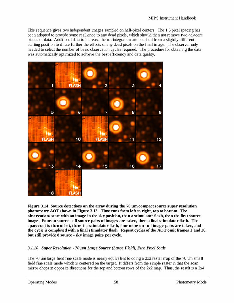
MIPS Instrument Handbook
Operating Modes 58
Photometry Mode
This sequence gives two independent images sampled on half-pixel centers. The 1.5 pixel spacing has been adopted to provide some resilience to any dead pixels, which should then not remove two adjacent pieces of data. Additional data to increase the net integration are obtained from a slightly different starting position to dilute further the effects of any dead pixels on the final image. The observer only needed to select the number of basic observation cycles required. The procedure for obtaining the data was automatically optimized to achieve the best efficiency and data quality.
Figure 3.14: Source detections on the array during the 70 µm compact source super resolution photometry AOT shown in Figure 3.13. Time runs from left to right, top to bottom. The observations start with an image in the sky position, then a stimulator flash, then the first source image. Four on source - off source pairs of images are taken, then a final stimulator flash. The spacecraft is then offset, there is a stimulator flash, four more on - off image pairs are taken, and the cycle is completed with a final stimulator flash. Repeat cycles of the AOT omit frames 1 and 10, but still provide 8 source - sky image pairs per cycle.
3.1.10 Super Resolution - 70 µm Large Source (Large Field), Fine Pixel Scale
The 70 µm large field fine scale mode is nearly equivalent to doing a 2x2 raster map of the 70 µm small field fine scale mode which is centered on the target. It differs from the simple raster in that the scan mirror chops in opposite directions for the top and bottom rows of the 2x2 map. Thus, the result is a 2x4
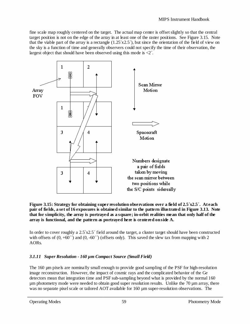
MIPS Instrument Handbook
Operating Modes 59
Photometry Mode
fine scale map roughly centered on the target. The actual map center is offset slightly so that the central target position is not on the edge of the array in at least one of the raster positions. See Figure 3.15. Note that the viable part of the array is a rectangle (1.25´x2.5 )́, but since the orientation of the field of view on the sky is a function of time and generally observers could not specify the time of their observation, the largest object that should have been observed using this mode is <2 .́
Figure 3.15: Strategy for obtaining super resolution observations over a field of 2.5´x2.5´. At each pair of fields, a set of 16 exposures is obtained similar to the pattern illustrated in Figure 3.13. Note that for simplicity, the array is portrayed as a square; in-orbit realities mean that only half of the array is functional, and the pattern as portrayed here is centered on side A. In order to cover roughly a 2.5´x2.5 ́field around the target, a cluster target should have been constructed with offsets of (0, +60´ )́ and (0, -60´ )́ (offsets only). This saved the slew tax from mapping with 2 AORs.
3.1.11 Super Resolution - 160 µm Compact Source (Small Field)
The 160 µm pixels are nominally small enough to provide good sampling of the PSF for high-resolution image reconstruction. However, the impact of cosmic rays and the complicated behavior of the Ge detectors mean that integration time and PSF sub-sampling beyond what is provided by the normal 160 µm photometry mode were needed to obtain good super resolution results. Unlike the 70 µm array, there was no separate pixel scale or tailored AOT available for 160 µm super-resolution observations. The

MIPS Instrument Handbook
Operating Modes 60
Photometry Mode
recommended method for specifying such an AOR using the available 160 µm pixel scale was an observation consists of 24 individual frames that provide three 2´x5.3 ́images, each containing 2 images of the source, with ½ pixel sampling in both the scan and cross-scan direction. The third image has the same cross-scan direction sampling of the PSF as the first image, but is placed on different pixels of the array to provide extra protection against unusual behavior of the Ge:Ga pixels and intra-pixel responsivity variations.
3.1.12 Total Power (TP) Mode
MIPS is optimized to provide calibrated images of sources that are small enough that they can be chopped on and off of the arrays, particularly at 70 and 160 µm. The Total Power (TP) mode AOT provides a way to accurately measure extended emission as well, by chopping between an internal dark position and the sky for each array. Experienced MIPS observers will note that the strategy for the 70 µm array changed from pre-launch expectations; now the 70 µm TP observations use side A of the array (the good side) and do indeed chop between the sky location to be measured (using the default 9.98´ ́pixel scale), and an internal dark position. The basic observation sequence begins with a frame at the dark position followed by a stimulator flash frame. Six more frames are taken at the dark position to allow the latent image from the stimulator flash to fade, then the scan mirror is used to change to the sky position, and a single image is taken of the source region. The scan mirror then moves back to the dark position, and 6 more frames are taken, allowing time for the latent image of the sky to fade. A final stimulator flash completes the cycle. This pattern (less the initial dark and stimulator flash frames) is repeated 5 times, providing 5 sky - dark image pairs per AOT cycle. This time-consuming process should provide excellent data on the germanium arrays. At 24 µm, image latents are better behaved. However, a 24 µm stimulator flash is included in this AOT (the only AOT that uses the 24 µm stimulator) in order to provide a reference signal for applying the droop correction to the data. This mode uses the same imaging arrays at 24, 70 and 160 micron, and therefore is affected by the same problems (see Chapter Chapter 7). Unlike standard photometry, this mode does not uses the scan mirror to dither between positions in the sky, and this adds additional problems with latencies (24 µm), and strong flux non-linearities (70 and 160 micron). Even for observers with experience with Ge:Ga detectors, this mode can be particularly difficult to deal with.
3.1.13 Photometry Raster Map
Scan maps are very efficient, and obtain data at all 3 wavelengths at once. However, for objects that are somewhat larger than 2 ́in diameter, but smaller than the 30 ́minimum scan map size, the photometry raster map option could be used to construct a map in one or more of the MIPS bands. The raster map uses the small field dither pattern identical to a single point Photometry/Super Resolution observation (same scan mirror and spacecraft offsets as described earlier). After completing observations in this fashion in a single field-of-view, the spacecraft is offset to an adjacent observer-specified field, and the normal photometry dither pattern is repeated. The observer specified the number of nearly-full-frame offsets in the along scan and cross-scan directions. The raster option returned high-quality 24 µm results because of the high stability of that array. Observers needed to specify offsets that gave some overlap between fields if they were interested in extended emission within the field of their raster map. For full coverage raster maps at 24 µm the observations should have used ½ array offsets, at most.
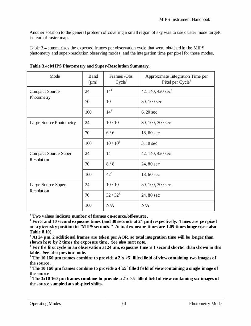
MIPS Instrument Handbook
Operating Modes 61
Photometry Mode
Another solution to the general problem of covering a small region of sky was to use cluster mode targets instead of raster maps. Table 3.4 summarizes the expected frames per observation cycle that were obtained in the MIPS photometry and super-resolution observing modes, and the integration time per pixel for those modes.
Table 3.4: MIPS Photometry and Super-Resolution Summary.
Mode Band (µm)
Frames /Obs. Cycle1
Approximate Integration Time per Pixel per Cycle2
Compact Source Photometry
24 143 42, 140, 420 sec4
70 10 30, 100 sec
160 145 6, 20 sec
Large Source Photometry 24 10 / 10 30, 100, 300 sec
70 6 / 6 18, 60 sec
160 10 / 106 3, 10 sec
Compact Source Super Resolution
24 14 42, 140, 420 sec
70 8 / 8 24, 80 sec
160 427 18, 60 sec
Large Source Super Resolution
24 10 / 10 30, 100, 300 sec
70 32 / 328 24, 80 sec
160 N/A N/A
1 Two values indicate number of frames on-source/off-source. 2 For 3 and 10 second exposure times (and 30 seconds at 24 µm) respectively. Times are per pixel on a given sky position in ''MIPS seconds.'' Actual exposure times are 1.05 times longer (see also Table 8.10). 3 At 24 µm, 2 additional frames are taken per AOR, so total integration time will be longer than shown here by 2 times the exposure time. See also next note. 4 For the first cycle in an observation at 24 µm, exposure time is 1 second shorter than shown in this table. See also previous note. 5 The 10 160 µm frames combine to provide a 2´x >5 ́filled field of view containing two images of the source. 6 The 10 160 µm frames combine to provide a 4´x5 ́filled field of view containing a single image of the source 7 The 3x10 160 µm frames combine to provide a 2´x >5´ filled field of view containing six images of the source sampled at sub-pixel shifts.

MIPS Instrument Handbook
Operating Modes 62
Large Area Mapping: Scan Mode
8 This indicates total number of frames, not total number of frames on-source (which is 8, just like the compact source).
3.2 Large Area Mapping: Scan Mode
3.2.1 Scan Map Mode
The scan map mode is designed to provide efficient mapping of large areas on the sky. A ramp motion of the scan mirror compensates for continuous telescope scanning motion, freezing the images on the arrays. The scan map mode avoids having to repoint and stabilize the telescope between exposures. A schematic representation of this is shown in Figure 3.16. Redundant images greatly improve the reliability of MIPS data, especially from the germanium arrays (e.g., to help remove cosmic ray effects, or uncertainties in the calibration of highly extended emission in a map). A single scan pass (or ''leg'') provides multiple redundancy at 24 and 70 µm (Figure 3.17). However, single scan legs provide only single redundancy at 160 µm at the slow and medium scan rates, and only 1/2 coverage at the fast scan rate (Figure 3.18 and Table 3.5). Redundant coverage at 160 µm, which was strongly recommended, could only be obtained if the observer specified at least two overlapping scan legs; it was strongly encouraged that observers obtain at least 4 images of a 160 µm target if the 160 µm data were important to the science goals. At 24 µm, another scan map at a later time was needed to identify asteroids; most asteroids at 70 µm should be identifiable by the ratio of their 24 and 70 µm colors. At all bands, a second map is desirable to remove transient events. It should be emphasized that the Scan Map AOT does not intrinsically provide any data redundancy at 160 µm at any scan rate. Those who wish to have high-quality scan data at 160 µm must use data with repeat coverage of the map area, either using sub-array scan leg offsets or repeat visits to the map area. See the discussion of data redundancy for the 160 µm Photometry AOT, section 3.1. As a result of the on-orbit realities with the Ge detectors, for full sky coverage at comparable signal-to-noise, it was recommended that observers should step by at most half-array widths (2.5 )́ in the cross-scan direction between scan legs. If 160 µm data was required, observers were instructed to design their observations to include sufficient redundancy at all locations in space, i.e., step by no more than 2.5 ́and preferably 2 ́to avoid the inoperative readout.
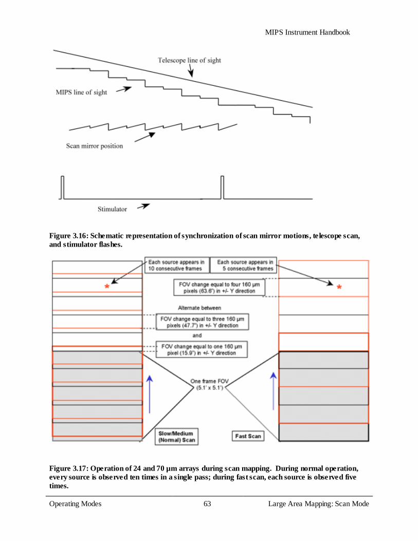
MIPS Instrument Handbook
Operating Modes 63
Large Area Mapping: Scan Mode
Figure 3.16: Schematic representation of synchronization of scan mirror motions, telescope scan, and stimulator flashes.
Figure 3.17: Operation of 24 and 70 µm arrays during scan mapping. During normal operation, every source is observed ten times in a single pass; during fast scan, each source is observed five times.

MIPS Instrument Handbook
Operating Modes 64
Large Area Mapping: Scan Mode
3.2.2 Telescope Motions
The telescope performs a scan at a constant rate. The observer could select from three discrete rates — slow, medium, and fast (approximately 2.6, 6.5, and 17.0 arcseconds per second). A scan leg is defined to be a single scan pass in one direction (forward or reverse). A scan map observation always starts in the ''forward'' direction (in the +Y direction in the Spitzer focal plane). The scan length is defined to be the distance along the scan track for which coverage is obtained with all three MIPS arrays. Scan lengths can be as short as 0.5° or as long as 6° (depending on the scan rate). There are regions of overscan at each end that have coverage by some of the arrays but not all. During the full-coverage portion of the observation, the telescope position should be within at least 1.3´ ́(rms) of the expected position along the scan track. At the end of a scan, the spacecraft pauses, then begins a new scan in the opposite direction to the first, with the same scan rate and either along the same track or offset by anywhere from 5´́ to 5 ́ in the cross-scan direction, as selected by the observer. For typical scan maps, scan legs can be assumed to be linear. Very long scans depart slightly from linear tracks. This curvature is determined by the offset between the arrays and the telescope centerline (X-axis), and any misalignment between the scan mirror rotation axis and the spacecraft Z-axis (Solar direction). Also, the scanned region on the sky is in general not exactly 90º from the line to the Sun, but can be anywhere within a 40º wide annulus .The net effect of these terms on the scan leg geometry is that the dominant direction of scan motion is a great circle centered on the spacecraft Z-axis. The motion is made such that the rotation is around a point 90º from the telescope boresight, and within 2º of the great circle centered on Spitzer and going through the center of the Sun. The pointing of the boresight is such that the scan leg centerline is positioned through the array centers. Perturbations that amount to small circle deviations are required to account for the focal plane layout and the actual scan mirror rotation axis relative to the Z-axis. The resultant curvature in the scan leg is <1% over a 6º scan. The relative pointing accuracy between two consecutive scan legs is expected to be ultimately better than 3´ ́(radial) for at least 4000 seconds time. During the course of an AOR, the Spitzer focal plane orientation on the sky is fixed. Therefore, there is no rotation of individual scan paths, nor is there any relative rotation between scan legs obtained within a single AOR. This holds in spite of the orbital motion of Spitzer during the period of the AOR. Scans obtained in separate AORs likely will have different orientations. The magnitude of the rotation depends on ecliptic latitude and time between AORs. To minimize such variations in scan orientation, observations may have to be constrained such that they are done within a short period of time, particularly when the targets are far away from the ecliptic. Please see Spitzer Telescope Manual for more information about spacecraft alignments, axes, and constraints.
3.2.3 Data Acquisition
At the start of the scan, the scan mirror is positioned near its ''center'' position, where all three detector arrays view the sky; data are collected from all three arrays. The scan mirror is moved in a one sided ramp with ''flyback'' around this position; during the ramp motion, the scan motion of the telescope is compensated by the motion of the scan mirror to freeze the field on the arrays. This operating mode is also called ''freeze frame scanning.'' The flyback occurs at intervals of 1 and 3 pixels of the 160 µm array alternately (i.e., ~16´ ́and 48´ )́ at the slow and medium scan rates, and every 4 pixels worth of slew at the fast rate (i.e., ~64´ )́. When the telescope scan direction is reversed, the parity of the scan mirror ramp/flyback is reversed. The pixel sizes for the stressed Ge:Ga (160 µm) and Si:As (24 µm) arrays provide good sampling of the telescope PSF. Improved sampling on a fractional pixel level in the scan direction is obtained on the 70 µm array as the source transits, because the frames are taken at non-integer
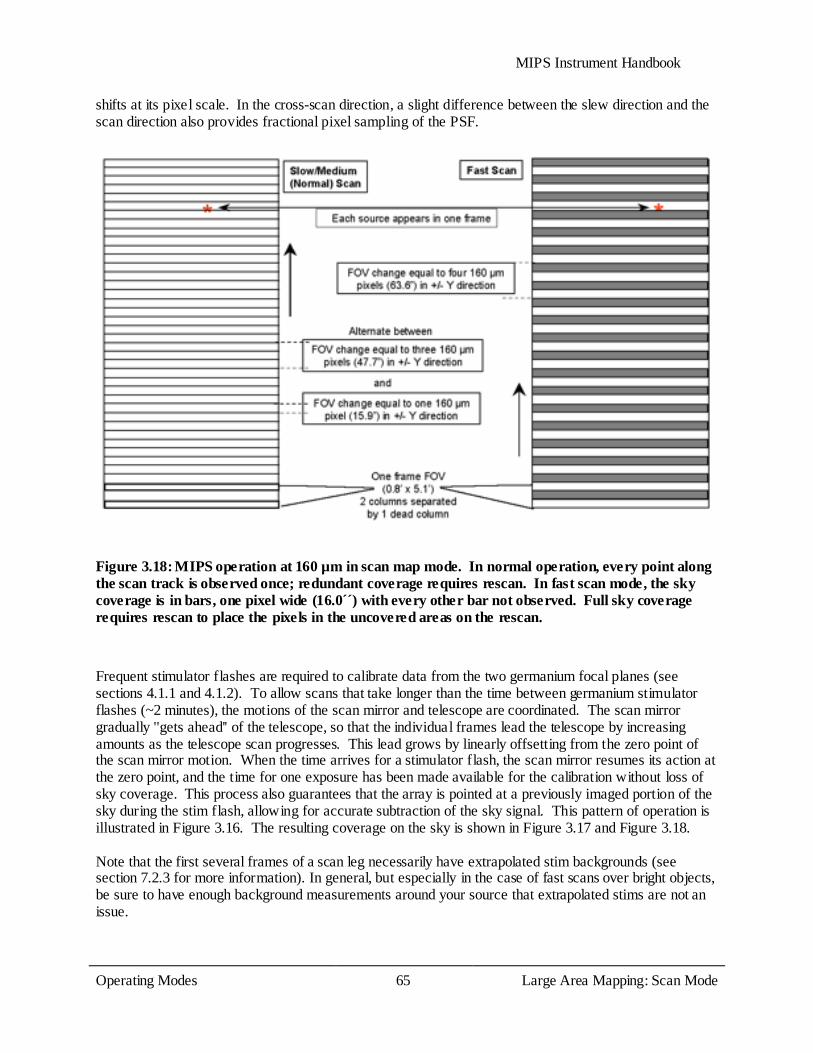
MIPS Instrument Handbook
Operating Modes 65
Large Area Mapping: Scan Mode
shifts at its pixel scale. In the cross-scan direction, a slight difference between the slew direction and the scan direction also provides fractional pixel sampling of the PSF.
Figure 3.18: MIPS operation at 160 µm in scan map mode. In normal operation, every point along the scan track is observed once; redundant coverage requires rescan. In fast scan mode, the sky coverage is in bars, one pixel wide (16.0´´) with every other bar not observed. Full sky coverage requires rescan to place the pixels in the uncovered areas on the rescan.
Frequent stimulator flashes are required to calibrate data from the two germanium focal planes (see sections 4.1.1 and 4.1.2). To allow scans that take longer than the time between germanium stimulator flashes (~2 minutes), the motions of the scan mirror and telescope are coordinated. The scan mirror gradually ''gets ahead'' of the telescope, so that the individual frames lead the telescope by increasing amounts as the telescope scan progresses. This lead grows by linearly offsetting from the zero point of the scan mirror motion. When the time arrives for a stimulator flash, the scan mirror resumes its action at the zero point, and the time for one exposure has been made available for the calibration without loss of sky coverage. This process also guarantees that the array is pointed at a previously imaged portion of the sky during the stim flash, allowing for accurate subtraction of the sky signal. This pattern of operation is illustrated in Figure 3.16. The resulting coverage on the sky is shown in Figure 3.17 and Figure 3.18. Note that the first several frames of a scan leg necessarily have extrapolated stim backgrounds (see section 7.2.3 for more information). In general, but especially in the case of fast scans over bright objects, be sure to have enough background measurements around your source that extrapolated stims are not an issue.

MIPS Instrument Handbook
Operating Modes 66
MIPS/SED Mode
3.2.4 Fast Scan Mode
Instrument operations at the fast scan rate (nominally about 17´ /́sec) are slightly different from those at the lower rates. Because the efficiency would be undesirably low at this scan rate if full sampling were obtained at 160 µm, that option is not supported and full coverage at this wavelength requires a second scan. The scan mirror flyback is set to four 160 µm pixel widths (64´ )́, with no alternation of flyback amplitudes. As a result, there is alternating one-pixel-wide gaps in 160 µm maps acquired in fast scan mode. Given that the pixels are 0.4 wide and separated by the same amount, any reasonably bright sources will be ''sighted'' at 160 µm even in the partial coverage obtained in a single pass. A general requirement for reliable scan maps is that the same area be scanned a second time (at a later date/time) to screen out asteroids and other transient phenomena. If a rescan is carried out very soon after the first, it can be approximately interleaved such that both scans together provide a nearly full 160 µm map. Note that the SSC strongly encouraged all observers to obtain at least 4 images of a 160 µm target if the 160 µm data was important, e.g., a forward and back scan leg over the same area with 2 map cycles, and with a 5-pixel offset in the cross-scan direction for fast scan (5 px compensates for the inoperable readout; see section 3.1. The total integration time per point on the sky per pixel in a single scan leg is provided in Table 3.5; overscan times are discussed further below in section 3.4.1.
Table 3.5: Total single-pass MIPS scan map integration time per pixel and overscan time.
Scan Rate 24 µm (sec)
Total / [time per frame]
70 µm (sec)
Total / [time per frame]
160 µm (sec) Overscan time (min)
Slow (2.6´́ /sec) 100 / [10] 100 / [10] 10 1.2 min
Medium (6.5´́ /sec) 40 / [4] 40 / [4] 4 3.2 min
Fast (17´́ /sec) 15 / [3] 15 / [3] 3 * 7.9 min
* Only 1/2 of map region is covered by the 160 µm pixels at the fast scan rate in one scan leg. Note: Each source appears in 10 consecutive frames for slow and medium scans at 24 and 70 µm, each source appears in 5 consecutive frames for fast scans at 24 and 70 µm, and each source appears in one frame at slow and medium scans at 160 µm. See Figure 3.17 and Figure 3.18.
3.3 MIPS/SED Mode
The Spectral Energy Distribution (SED) mode applies only to the 32x32 Ge:Ga array, since it requires an offset of the scan mirror that deflects light away from the optical trains for the other arrays. This operating mode provides long-slit, low-resolution (R ~ 15-25) spectra in the far infrared (52 - 97 µm), with a dispersion of 1.70 µm /pix via a reflection grating. The SED optical train illuminates a slit approximately two detector pixels (~20´ )́ wide and 12 pixels (~2 )́ long where the full wavelength coverage is available. An inoperative detector module at the blue end of the dispersion of side A restricts

MIPS Instrument Handbook
Operating Modes 67
MIPS/SED Mode
the wavelength coverage to only 65 - 97 µm over the last 4 columns of the 16x32 detector array. Only side A data is calibrated for the SED mode. A standard SED observation provides pairs of data frames between the target position (ON) and a nearby sky position (OFF). The scan mirror is used to chop between the ON and OFF, and an observer can choose a chop throw of +3´, +2´, +1 ,́ or -1 .́ The observer can request either a pointed observation or an MxN raster map (with M, N between 1 and 100). For a pointed observation (or at each raster position in the case of a raster map), there is a basic set of 6 pairs of ON and OFF frames (plus bracketing frames on the internal stimulator (for tracking detector responsivity variations), of which the first 3 pairs are obtained with the target placed near the center of detector column 10 (hereafter referred to as dither position 1) and the next 3 pairs with the target near the center of column 5 (dither position 2). The observer repeats this basic observing set by a number of cycles (NC) in order to reach the desired S/N ratio. For a mapping observation, the value of NC remains the same for all the raster positions. Using the same detector and internal stimulators, the SED mode shares some calibration characteristics (e.g., dark current) with the 70 µm imaging mode. As a result, most discussion on the data products and general detector calibration of the 70 µm imaging mode in this handbook applies directly to the SED mode. SED observations provide pairs of data frames with the target in the slit and at a nearby off position. The scan mirror is used to chop between the target and the off position, and the observer can pick a chop throw of +3´, +2´, +1´, or -1 .́ An SED observation begins with an image at the off position followed by a stimulator flash frame. The scan mirror brings the target into the slit, and a series of 3 target - sky image pairs is taken with the scan mirror chopping between the two positions. The series ends with a stimulator flash frame following the final sky frame. The telescope then nods to move the target along the slit to a second position, and the above sequence of images, stimulator flashes, and scan mirror motions is repeated. If additional integration time is needed, the sequence is repeated except that the first sky - stim flash pair of frames is omitted. Consequently the AOT provides 6 target - sky image pairs per cycle; see Figure 3.19. The observer specified only the total number of basic observation cycles required; the number of pairs to be taken at one spacecraft setting before offsetting to the other has been optimized, as with the photometry mode.
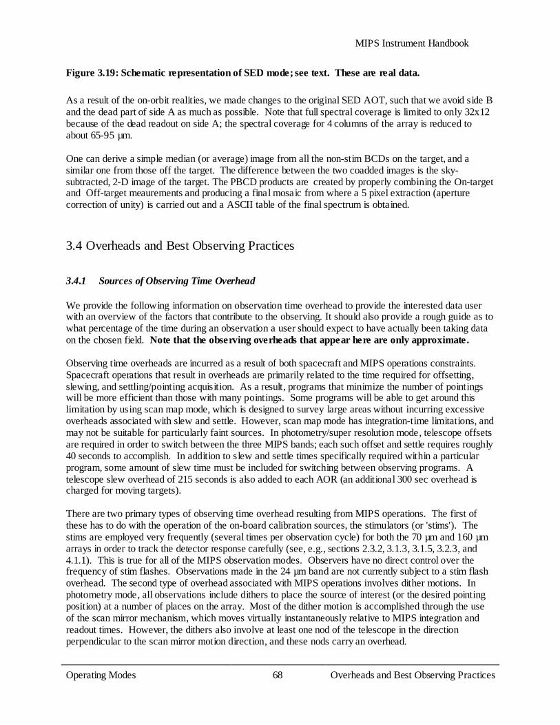
MIPS Instrument Handbook
Operating Modes 68
Overheads and Best Observing Practices
Figure 3.19: Schematic representation of SED mode; see text. These are real data. As a result of the on-orbit realities, we made changes to the original SED AOT, such that we avoid side B and the dead part of side A as much as possible. Note that full spectral coverage is limited to only 32x12 because of the dead readout on side A; the spectral coverage for 4 columns of the array is reduced to about 65-95 µm. One can derive a simple median (or average) image from all the non-stim BCDs on the target, and a similar one from those off the target. The difference between the two coadded images is the sky-subtracted, 2-D image of the target. The PBCD products are created by properly combining the On-target and Off-target meaurements and producing a final mosaic from where a 5 pixel extraction (aperture correction of unity) is carried out and a ASCII table of the final spectrum is obtained.
3.4 Overheads and Best Observing Practices
3.4.1 Sources of Observing Time Overhead
We provide the following information on observation time overhead to provide the interested data user with an overview of the factors that contribute to the observing. It should also provide a rough guide as to what percentage of the time during an observation a user should expect to have actually been taking data on the chosen field. Note that the observing overheads that appear here are only approximate. Observing time overheads are incurred as a result of both spacecraft and MIPS operations constraints. Spacecraft operations that result in overheads are primarily related to the time required for offsetting, slewing, and settling/pointing acquisition. As a result, programs that minimize the number of pointings will be more efficient than those with many pointings. Some programs will be able to get around this limitation by using scan map mode, which is designed to survey large areas without incurring excessive overheads associated with slew and settle. However, scan map mode has integration-time limitations, and may not be suitable for particularly faint sources. In photometry/super resolution mode, telescope offsets are required in order to switch between the three MIPS bands; each such offset and settle requires roughly 40 seconds to accomplish. In addition to slew and settle times specifically required within a particular program, some amount of slew time must be included for switching between observing programs. A telescope slew overhead of 215 seconds is also added to each AOR (an additional 300 sec overhead is charged for moving targets). There are two primary types of observing time overhead resulting from MIPS operations. The first of these has to do with the operation of the on-board calibration sources, the stimulators (or 'stims'). The stims are employed very frequently (several times per observation cycle) for both the 70 µm and 160 µm arrays in order to track the detector response carefully (see, e.g., sections 2.3.2, 3.1.3, 3.1.5, 3.2.3, and 4.1.1). This is true for all of the MIPS observation modes. Observers have no direct control over the frequency of stim flashes. Observations made in the 24 µm band are not currently subject to a stim flash overhead. The second type of overhead associated with MIPS operations involves dither motions. In photometry mode, all observations include dithers to place the source of interest (or the desired pointing position) at a number of places on the array. Most of the dither motion is accomplished through the use of the scan mirror mechanism, which moves virtually instantaneously relative to MIPS integration and readout times. However, the dithers also involve at least one nod of the telescope in the direction perpendicular to the scan mirror motion direction, and these nods carry an overhead.

MIPS Instrument Handbook
Operating Modes 69
Overheads and Best Observing Practices
The photometry mode dithers cannot be circumvented by observers. These required dither patterns are designed to improve the accuracy of MIPS photometry by placing sources at several positions on the detectors (both 70 and 160 µm arrays), and to provide a filled 2-D image for the 160 µm array. While the dithering does not result in an observing overhead per se, it does mean that the minimum integration time on a source is a function of the product of the observer-selected exposure time and the number of dither positions. For bright sources, these minimum integration times might exceed the integration time required by a significant amount.
3.4.2 Fractional Observing Time Overhead
Here we provide illustrative values that can be used for estimating the observing time required to complete an observation given the integration time required to achieve the desired signal-to-noise on a source. The observing times derived here are approximate and were subject to small changes. The amount of overhead incurred in making an observation can conveniently (if approximately) be represented as a factor which, when multiplied by the desired integration time, gives the observing overhead time. The total observation time (or total observation ''wall clock time'') is just the integration time plus the overhead time, and can be represented as:
Observing Time = (1 + overhead factor) x Integration Time (3.1)
Table 3.6: Approximate overhead factors for MIPS photometry/super-resolution (small field option).
Exposure Time (MIPS sec), Band First-Cycle Integration Time (sec)
First-Cycle Overhead
Factor
Seven-Cycle Integration Time (sec)
Seven-Cycle Overhead
Factor
3 sec, 24 µm 48 1.40 312 0.36
10 sec, 24 µm 166 0.41 1046 0.11
30 sec, 24 µm 501 0.13 3144 0.04
3 sec, 70 µm (coarse scale) 38 2.07 226 0.68
10 sec, 70 µm (coarse scale) 126 0.85 881 0.38
3 sec, 70 µm (fine scale) 25 4.47 176 2.03
10 sec, 70 µm (fine scale) 84 2.57 587 1.53
3 sec, 160 µm 6 22.13 44 12.19
10 sec, 160 µm 21 12.99 147 8.39
3 sec, 160 µm (enhanced) 13 30.6 107* 11.0*
MIPS Instrument Handbook
Operating Modes 70
Overheads and Best Observing Practices
10 sec, 160 µm (enhanced) 45 14.1 357* 8.9*
* Cycles 7, 11, 13, 17, and 19 are not allowed in 160 µm enhanced mode. The numbers given in the table are for 8 cycles.
In Table 3.6, we tabulate the overhead factors for observations taken in photometry/super resolution mode for the available MIPS exposure times. Note that the tabulated integration times are in real time seconds, not ''MIPS seconds'' (see section 2.4). While the combination of dither patterns and minimum exposure time results in fairly long minimum effective integration times, almost any arbitrary integration time longer than the minimum can be obtained by combining sets of 7-cycle observations with single-cycle observations. For most dither patterns, for cycles up to 7 there is only one spacecraft offset, with all other dithers being done with the scan mirror. This is to minimize accumulated overhead caused by unnecessarily repeating motions that require slew and settle overheads, while scan mirror motions do not. For more than 7 cycles, the number of spacecraft motions depends on the natural break points in the sequence. For the purposes of estimation of observing times, the simple method described here will give adequate results. Note that for purposes of determining whether a source will saturate the MIPS detectors, the exposure time matters, while for purposes of calculating signal-to-noise ratios, integration time is the appropriate quantity to consider. Note also that these overhead factors are for observations in a single band; if multiple wavelengths are desired, an additional 40 second overhead is incurred for offsetting the spacecraft to bring the object into view of each additional band. Observing overheads for scan map mode are somewhat more difficult to summarize than are those for photometry mode. Because the three MIPS arrays view different areas of the sky, the length of a scan leg must be somewhat longer than the length of the region being mapped. The overscan distance required to obtain a 3-wavelength full-coverage map is about 20.7 .́ Data are obtained in the overscan region, but are not co-spatial in all 3 bands, and might have somewhat larger than usual pointing uncertainties in the first several frames. While viable science data, the time spent covering the overscan region is considered observing overhead. The amount of overhead depends on the scan rate selected by the observer, as summarized in Table 3.5. Exposure times in scan-map mode are determined by the scan rate selected. Likewise, the integration time on any particular point in the scan-map is also determined by the selected scan rate, although deeper integrations can be obtained by re-scanning a region and coadding the resulting maps. The exposure and integration times for the three MIPS arrays as a function of scan rate are detailed in section 3.2, and that section should be referred to in order to estimate sensitivity as a function of flux, and saturation fluxes as a function of scan rate. The length of time required to complete a 5 ́wide scan leg is just the length of the leg divided by the scan rate (including the overscan distance). If the region to be mapped is wider than 5 ́(2.5 ́for full 70 µm coverage), the map must be built up by specifying multiple scan legs, including specifically some overlap between those legs to ensure complete coverage of the region at all wavelengths. Each time a scan leg finishes and a new scan leg is begun, an overhead of about 30 to 60 seconds for ''turnaround time'' (time to stop the scan and begin set up of the new scan leg), which includes an offset and settle, is incurred. There is also a 30 second overhead incurred at the beginning of each scan map AOR for establishing initial pointing, settling, and beginning to slew.

MIPS Instrument Handbook
Operating Modes 71
Overheads and Best Observing Practices
3.4.3 Best Observing Practices
Below are summaries of the recommended Best Observing Practices at the time of the data acquisition. This does not imply that data taken in another way are inferior in any way. In many cases these general rules either did not apply to a particular observation or made no difference one way or another. Often the practices merely ensured time efficient data acquisition, which would be of little relevance to an archive user. However, if Best Observing Practices were not followed it is possible the data might not be as sensitive or well calibrated as other comparable data, so we recommend the user try to understand why (or why it does not matter) the Best Observing Practices were ignored. Also be sure to check Data Features and Artifacts for other possible issues the data may contain.
Best Observing Practices: General MIPS
For far infrared Ge detectors, observers should make sure they take enough background (source-free) data. For large sources we recommend using the chopping large-field photometry mode or scan mapping. At 160 µm we recommend using the new 160 µm enhanced photometry mode for small sources. At least four images of a 160 µm target are recommended to ensure reliable photometry. Images of objects near the ecliptic plane are likely to include asteroids and/or Kuiper Belt objects; a second observation at a later time is necessary to ensure that moving targets have been removed. Observations at MIPS wavelengths may be limited by noise (including confusion noise; see section 2.5.1) but observers should ensure sufficient data redundancy for cosmic ray rejection, even if the confusion limit is reached with shorter exposures. It is best to build up long integrations with long exposure times, e.g. large total integration times built from 3 s exposures will not produce as high-quality a final product as fewer cycles of 10 s exposures.
Best Observing Practices: MIPS Photometry
In addition to the items mentioned immediately above for MIPS in general, observers should also consider the following items relevant specifically to MIPS photometry. Super-resolution data needs to be post-processed to take advantage of the sub-pixel sampling inherent in the AOT; the Spitzer pipelines do not provide this service. In photometry observations, the dither pattern is such that the region of highest-quality S/N and best coverage is less than a full FOV; be sure to visualize the exposures to determine the region of sky actually covered by all pointings for any given AOR. Because of the smaller effective size of the 70 µm array compared to original expectations, to obtain the same coverage as pre-launch expectations for large-field photometry, some users needed to efficiently map the approximately 5´x5 ́(2.5´x2.5 ́fine scale) area covered by the original AOT. In order to do this, we suggested that the user create a cluster target with offsets of (0, +80´ )́, (0, -80´ )́ [for fine scale, (0, +60´ )́, (0, -60´ )́] in array coordinates observing ''offsets only.'' This allowed recovery of the full area of the original AOT while saving the slew tax from mapping with 2 AORs.
Best Observing Practices: Scan
MIPS Instrument Handbook
Operating Modes 72
Overheads and Best Observing Practices
In addition to the items mentioned immediately above and for MIPS in general, observers should also consider the following items relevant specifically to MIPS scans. Step by at most 1/2 array steps to obtain full sky coverage at all 3 wavelengths. For the best data at 70 µm we recommend cross-scan steps of <= 148´ .́ For highest S/N coverage, step by at most ¼ array steps. The AOT provides inherent redundancy in all wavelengths, but there are more images of a given source at 24 and 70 µm than at 160 µm. Fast scans provide only half coverage at 160 µm, so the scans must be repeated to approximately fill in the gaps. To achieve the recommended minimum 4 images of the same patch of sky, observers should plan additional scans with small cross-scan steps. Bright objects may leave latents in the data; to limit these effects, an observer should arrange to cover the same region of the sky in two directions (e.g., forward and back). A user may want to isolate extremely bright objects in a separate AOR. Note that the first several frames of a scan leg necessarily have extrapolated stim backgrounds (see section 7.2.3 for more information on this effect). In general, but especially in the case of fast scans over bright objects, an observer should be sure to have enough background measurements around your source so that extrapolated stims are not an issue.
Best Observing Practices: SED
In addition to the items mentioned above for MIPS in general, observers using MIPS SED mode need to consider their exposure times and likelihood of saturation. Since the saturation limits are so high for the 70 µm array, it's rare to saturate SED mode. Thus, except in situations where extremely bright objects are being observed, one should always use the 10 second exposure time.

MIPS Instrument Handbook
Calibration 73
Imaging
Chapter 4 Calibration
For all information on calibration of MIPS data one should refer to the published MIPS calibration papers: 24 microns (Engelbracht et al. 2007, PASP, 119, 994), 70 microns (Gordon et al. 2007, 119, 1019), 160 microns (Stansberry et al. 2007, PASP, 119, 1038), and MIPS SED (Lu et al. 2008, PASP, 120, 328).
4.1 Imaging
4.1.1 Methodology MIPS 24 and 70 micron arrays are calibrated using primary (routine) stars and secondary calibrator stars. See the individual calibration papers for specific methodology for each camera. Because of the near infrared filter leak at 160 µm, asteroids (primary calibrators) and red extragalactic sources (secondary calibrators) are used instead of stars (see Stansberry et al. 2007). The routine stars are used to monitor stability of the array in the absolute calibration. For routine stars, we use HD159330 (which is a K star) at 24 microns, and HD163588 and HD180711 star for 70 and 160 microns (for repeatability). These stars are observed at least once every 3 days. The secondary stars have been chosen from our MIPS calibrator list of about 150 stars. Star on this list are bright enough (S/N > 100) and well within the linear range of the detector, i.e., less than 1/4 of the saturation limit. Most of the calibrators are located in regions of low cirrus background, but there are a few stars with a high background in order to test photometry in high background conditions. We present a large representative sample composed of all calibration observations through the 42nd MIPS campaign (~2/3 of the total cryogenic mission) in Table 4.1. Note that the 160 micron stars are affected by the spectral leak, and thus used for stability and templates, not flux calibration. A complete list of MIPS calibrators can also be found with the Calibration and Data Analysis Files on this website. To retrieve actual calibration observations, if you don't know specific names of targets, then you need a program id (pid) to retrieve the entire MIPS calibration program for a given campaign. MIPS calibrations are assigned a PID = 1700+MIPS campaign number. For example, MC 7 corresponds to 1710 and MC 18 to 1721, etc. These campaigns should include calibration for everything (all MIPS modes), so you have to investigate the specific AORs to find ones that match your needs. MIPS calibrations are done every campaign, so you should be able to start with downloading just one. If the data are not accessible from a given observation, it is most likely because there is an approved science program that is also observing that target in that mode.
Table 4.1: A Representative Sample of Calibrators Used.
Mode Total Unique Flux range (Jy)
Types (A/G/K/M/F/B)
24 micron 372 103 0.086-4.0 34/25/39/0/2/3
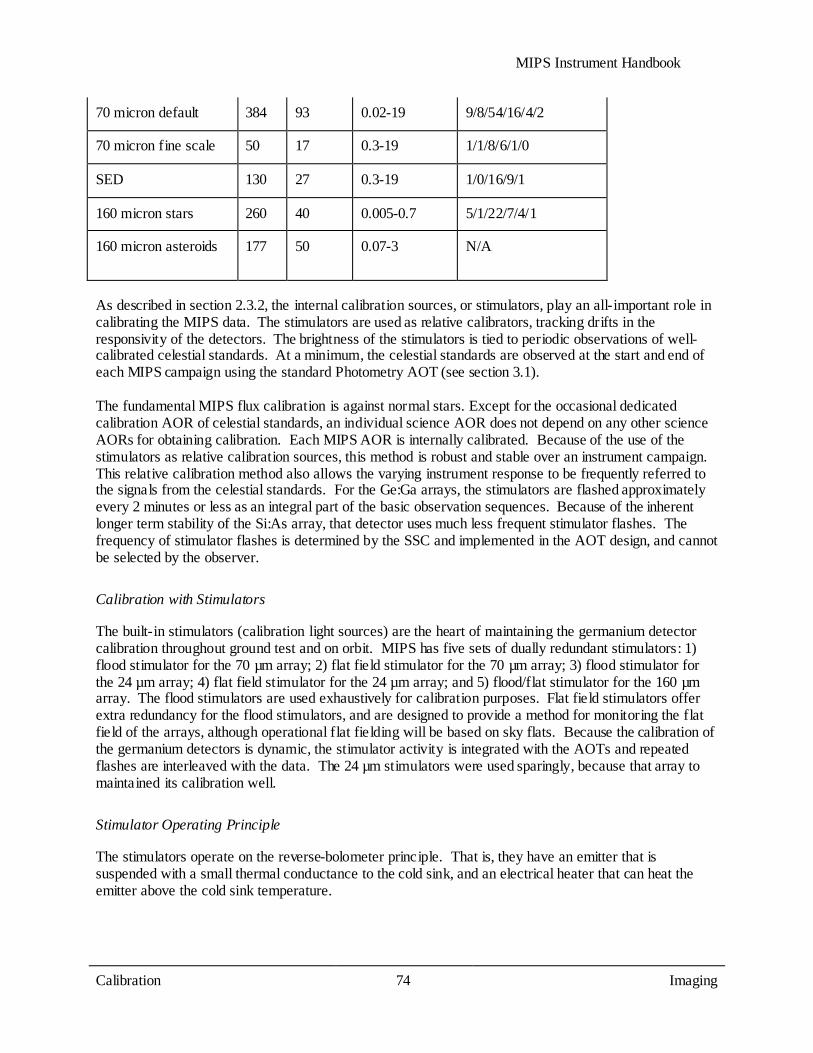
MIPS Instrument Handbook
Calibration 74
Imaging
As described in section 2.3.2, the internal calibration sources, or stimulators, play an all-important role in calibrating the MIPS data. The stimulators are used as relative calibrators, tracking drifts in the responsivity of the detectors. The brightness of the stimulators is tied to periodic observations of well-calibrated celestial standards. At a minimum, the celestial standards are observed at the start and end of each MIPS campaign using the standard Photometry AOT (see section 3.1). The fundamental MIPS flux calibration is against normal stars. Except for the occasional dedicated calibration AOR of celestial standards, an individual science AOR does not depend on any other science AORs for obtaining calibration. Each MIPS AOR is internally calibrated. Because of the use of the stimulators as relative calibration sources, this method is robust and stable over an instrument campaign. This relative calibration method also allows the varying instrument response to be frequently referred to the signals from the celestial standards. For the Ge:Ga arrays, the stimulators are flashed approximately every 2 minutes or less as an integral part of the basic observation sequences. Because of the inherent longer term stability of the Si:As array, that detector uses much less frequent stimulator flashes. The frequency of stimulator flashes is determined by the SSC and implemented in the AOT design, and cannot be selected by the observer.
Calibration with Stimulators
The built-in stimulators (calibration light sources) are the heart of maintaining the germanium detector calibration throughout ground test and on orbit. MIPS has five sets of dually redundant stimulators: 1) flood stimulator for the 70 µm array; 2) flat field stimulator for the 70 µm array; 3) flood stimulator for the 24 µm array; 4) flat field stimulator for the 24 µm array; and 5) flood/flat stimulator for the 160 µm array. The flood stimulators are used exhaustively for calibration purposes. Flat field stimulators offer extra redundancy for the flood stimulators, and are designed to provide a method for monitoring the flat field of the arrays, although operational flat fielding will be based on sky flats. Because the calibration of the germanium detectors is dynamic, the stimulator activity is integrated with the AOTs and repeated flashes are interleaved with the data. The 24 µm stimulators were used sparingly, because that array to maintained its calibration well.
Stimulator Operating Principle
The stimulators operate on the reverse-bolometer principle. That is, they have an emitter that is suspended with a small thermal conductance to the cold sink, and an electrical heater that can heat the emitter above the cold sink temperature.
70 micron default 384 93 0.02-19 9/8/54/16/4/2
70 micron fine scale 50 17 0.3-19 1/1/8/6/1/0
SED 130 27 0.3-19 1/0/16/9/1
160 micron stars 260 40 0.005-0.7 5/1/22/7/4/1
160 micron asteroids 177 50 0.07-3 N/A
MIPS Instrument Handbook
Calibration 75
Imaging
Stimulator Usage in MIPS
The flat field stimulator for the 70 µm array is at the focus of a projector that re-images it onto the scan mirror, which is at a pupil in the optical system. The output can be directed through the wide-field 70 µm imaging optical train or through the SED optical train by suitably positioning the scan mirror. The projector is required so flat fields can be obtained for imaging and spectroscopic modes independently (i.e., without light going through both optical trains). Geometric constraints prevent light from the flat field stimulator from being directed into the high-resolution 70 µm imaging train. The 24 µm flat field stimulator is located in an integrating cavity and its output is conveyed through a machined aluminum light pipe to an exit pinhole at a pupil near the array. The 160 µm stimulator is also in an integrating cavity with a small exit hole in a mirror at a pupil, placed right in front of the concentrators that convey the light to the detectors. The flat fields obtained using the flat field stimulators within MIPS are periodically calibrated against observations of a uniform region of the sky. The flood stimulators at 24 and 70 µm are close to the detectors and broadcast light in a less controlled manner than the flat field stimulators. They are used primarily for relative calibration, while the 160 µm stimulator is used for both calibration and flat fielding. For observations taken with the 70 and 160 µm arrays, frequent (~2 minute interval) brief (~2 second) stimulator flashes automatically occur during data taking, both during observations of reference flux standards and science observations. The resulting signal from these stimulator flashes provides a continuous measure of the responsivity of each pixel in these arrays. Observers could not control the rate or placement of the stim flashes. Pipeline processing of the data uses the stimulator flashes to remove long-term changes in responsivity, and provides a relative calibration source for referencing all science observations to flux standards.
Dark Current
As part of instrument calibration, dark current must be periodically measured for each array. This is done at the beginning and end of each instrument campaign, similar to observations of the flux calibration stars. The scan mirror has positions which do not allow light to fall on the arrays, and these positions are used, in part, for dark current measurements. The dark current is measured immediately after an anneal, before the detector responsivity has had time to change due to cosmic ray hits. Detector dark current measurements are made for each array individually by positioning the scan mirror such that the array views only the interior of the cold instrument. The optical layout of MIPS is such that only one array at a time can be completely hidden from light entering through the telescope. In fact, only about two thirds of the 70 µm array can be placed in the dark at once, so for that array the dark current measurement is made in two pieces. Dark current measurements are expected to only be required at the beginning and end of each MIPS campaign. To avoid any scattered light from nearby very bright sources affecting the measurement, the telescope is pointed toward a region known to be free of such sources during the dark current measurement sequence.
Summary
The MIPS calibration consists of measurements of a number of candidate calibration stars. From these data, we have made a selection of fundamental calibrator stars. At the beginning and end of a MIPS observing campaign, we observe one or more fundamental calibrator stars, establishing the absolute flux calibration for the internal stimulators. Frequent observations of the brightness of the stimulators are used
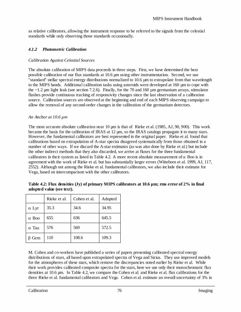
MIPS Instrument Handbook
Calibration 76
Imaging
as relative calibrators, allowing the instrument response to be referred to the signals from the celestial standards while only observing those standards occasionally.
4.1.2 Photometric Calibration
Calibration Against Celestial Sources
The absolute calibration of MIPS data proceeds in three steps. First, we have determined the best possible calibration of our flux standards at 10.6 µm using other instrumentation. Second, we use ''standard'' stellar spectral energy distributions normalized to 10.6 µm to extrapolate from that wavelength to the MIPS bands. Additional calibration tasks using asteroids were developed at 160 µm to cope with the ~1.2 µm light leak (see section 7.2.6). Finally, for the 70 and 160 µm germanium arrays, stimulator flashes provide continuous tracking of responsivity changes since the last observation of a calibration source. Calibration sources are observed at the beginning and end of each MIPS observing campaign to allow the removal of any second-order changes in the calibration of the germanium detectors.
An Anchor at 10.6 µm
The most accurate absolute calibration near 10 µm is that of Rieke et al. (1985, AJ, 90, 900). This work became the basis for the calibration of IRAS at 12 µm, so the IRAS catalogs propagate it to many stars. However, the fundamental calibrators are best represented in the original paper. Rieke et al. found that calibrations based on extrapolation of A-star spectra disagreed systematically from those obtained in a number of other ways. If we discard the A-star estimates (as was also done by Rieke et al.) but include the other indirect methods that they also discarded, we arrive at fluxes for the three fundamental calibrators in their system as listed in Table 4.2. A more recent absolute measurement of α Boo is in agreement with the work of Rieke et al. but has substantially larger errors (Witteborn et al. 1999, AJ, 117, 2552). Although not among the Rieke et al. fundamental calibrators, we also include their estimate for Vega, based on intercomparison with the other calibrators.
Table 4.2: Flux densities (Jy) of primary MIPS calibrators at 10.6 µm; rms error of 2% in final adopted value (see text).
Rieke et al. Cohen et al. Adopted
α Lyr 35.3 34.6 34.95
α Boo 655 636 645.5
α Tau 576 569 572.5
β Gem 110 108.6 109.3
M. Cohen and co-workers have published a series of papers presenting calibrated spectral energy distributions of stars, all based upon extrapolated spectra of Vega and Sirius. They use improved models for the atmospheres of these stars, which remove the discrepancies noted earlier by Rieke et al. While their work provides calibrated composite spectra for the stars, here we use only their monochromatic flux densities at 10.6 µm. In Table 4.2, we compare the Cohen et al. and Rieke et al. flux calibrations for the three Rieke et al. fundamental calibrators and Vega. Cohen et al. estimate an overall uncertainty of 3% in

MIPS Instrument Handbook
Calibration 77
Imaging
their results (Cohen et al. 1996, AJ, 112, 2274). The Cohen values in Table 4.2 reflect a 0.6% upward revision of their fluxes, as suggested by a recent revision in the calibration of Vega at V (Megessier, 1997, Proc. IAU Symp. 189, p. 153), with an accompanying downward revision of their uncertainty to ~2.5%. The most important result in Table 4.2 is that the two calibration approaches are in excellent agreement for all three calibrators (and Vega). Since the quoted errors for both groups are nearly identical, it is appropriate to take the straight average of the fluxes from the two approaches, and to assign an rms error of 2% to the result.
Extrapolation to the MIPS Bands
To guard against systematic errors, we use three independent methods to extrapolate the calibration to the MIPS bands: 1) Solar Analog method; 2) extrapolation with A star atmospheric models; and 3) extrapolation with semi-empirical models of red giants. Additional tasks at 160 µm use asteroids; see below.
Solar Analogs
Johnson introduced a method of absolute calibration in which direct comparisons of the Sun and calibrated blackbody sources are transferred to a network of ''solar analog'' stars of type similar to the Sun. The flux offset between the Sun and these stars is assumed to be equal to their brightness difference at some readily measured wavelength (e.g., V band). This method has been used by Campins et al. (1985, AJ, 90, 896) and further references can be found there. One unique aspect of the application of this method to MIPS is that it is the only feasible ''direct'' calibration, in which the data can be referred back to a comparison with a calibrated laboratory source at or near the wavelength of interest, without relying on spectral extrapolation. Calibration using the solar-type stars is accomplished by using the empirical fit to the measured solar spectrum Engelke 1992, AJ, 104, 1248) to extrapolate solar-type spectra through the MIPS bands. Because of the small differences in stellar temperature, and the minimal line blanketing in the far infrared, the Engelke approximation should be very accurate.
A-Star Model Atmospheres
A-type stars are popular for extrapolating calibrations because it is believed that their atmospheres are relatively straightforward to model. They are probably the most reliable way to extend the MIPS calibration by comparison with theory. A large number of A-stars can be easily measured at 70 µm, and many more (excepting Sirius, which will saturate) can be measured at 24 µm. The foundation for this approach is accurate atmospheric models, such as those available for Sirius and Vega. Vega itself cannot be used as a calibrator because of its bright debris disk, and a comparison among the measurements of a number of stars will be necessary to identify those without any contamination by disk excesses. Fortunately, enough A-type and solar type stars are available to allow us to reject sources with disk-induced far-IR excesses by simple comparison with the median fluxes of the ensemble of sources.
Red Giants

MIPS Instrument Handbook
Calibration 78
Imaging
Red giants generally have very complex atmospheres and are not favored for extrapolation of calibrations. However, in the far-infrared, their spectra appear to exhibit simple Rayleigh-Jeans-like behavior, as shown by the extensive set of composite spectra assembled by Cohen and co-workers. Thus, the brightest red giants play a critical role in the calibration in the far infrared. Unfortunately these sources saturate the 24 µm array. To cross-calibrate the bright giants with the shorter-wavelength A and G star calibration, it is necessary to observe a group of fainter red giants at 24 µm, and then assume that their spectra are identical to the bright giant spectra for stars of identical spectral type.
160 µm Light Leak and Calibrations
During IOC/SV, 160 µm signals from K stars were detected to be about a factor of five stronger than expected. Review of the instrument design revealed a weakness in the stray light control resulting in a short-wavelength (1-1.6 µm) light leak in this band. As a result, there was a reworking of the calibration plans for this waveband. Asteroids are now used as the primary celestial 160 µm calibrators. Asteroids are observed at both 70 and 160 µm (with some also observed at 24 µm), and so the 70 µm channel provides a link to 160 µm via asteroid models. This is similar to the IRAS 100 µm calibration strategy. Secondary calibrators at 160 µm include leak-subtracted stars, debris disks, extended targets such as galaxies and planetary nebulae, and ISO surveys. For many types of observations, this light leak does not impact the data at all. Stars fainter than mJ ~ 5.5 mag will not be detectable in the leak above the confusion level. No compact extragalactic sources have mJ brighter than 5.5 mag. The leak signal for a star of mJ = -0.5 mag is equivalent to ~ 2.5 Jy at 160 µm. The parameter to consider for any given target is the 160 µm /2 µm flux density ratio. For a Rayleigh-Jeans source, this ratio is 0.0001. Anything with a ratio larger than 0.004 will produce uncorrupted data, so most objects will not be affected. Sources with 160 µm fluxes more than a factor of 40 above that of a Rayleigh-Jeans source from 1 - 1.6 µm will have leak signals <10% at 160 µm. Galactic programs on star formation, ISM, etc., will likely be impacted. It has been demonstrated that observations of bright point sources strongly impacted by the leak (stars) can be corrected to a high level using an empirical stellar PSF and careful deconvolution (see, e.g., Stapelfeldt et al. 2004, ApJS, 154, 458). Best results will be obtained with observations for which proper planning and data acquisition was made to allow a good characterization of the leak signature for the object brightness and color. For example, plan to obtain identical observations of ''calibrator'' stars of similar type and brightness to your target stars, but without long-wavelength excesses. For stellar observations, the strongest signal apparent in a 160 µm observation is likely to be the leak itself. Tests were performed using HD 163588, a K2III star that is routinely observed at 70 µm and has also been observed at 160 µm. Similar results are obtained for HD 36673 (Arneb), an F0Ib star, and for HD 87901 (Regulus), a B7V star. The leak is 15±7 times as bright as the photosphere of a star. Example images are presented in Data Features and Artifacts.
Filter Blocking
Using normal stars as calibrators imposes severe requirements on the understanding of near-infrared filter leaks. Leaks were measured by comparing the beam profiles of observations of asteroids and stars. If there had been filter leaks, the stellar point spread function would have included spatial frequencies appropriate to the near-infrared Airy pattern of the telescope, frequencies which physically cannot be associated with a true far-infrared signal. Because the ratio of near-infrared to far-infrared flux is much lower for asteroids than for stars, near-IR filter leaks are negligible for the asteroids. Therefore, a careful
MIPS Instrument Handbook
Calibration 79
Imaging
comparison of PSFs can reveal filter leaks and allow us to measure them. Spatial power spectra of the PSFs can clearly separate the two frequency components if they are present. This method is described by Kirby et al. (1994, AJ, 107, 2226).
4.1.3 Uncertainties and Repeatability
We derived the flux conversion using both primary and secondary stars by fitting the relationship between predicted flux and DN. We have to rely on models to predict the fluxes at MIPS bands. Kurucz models are used for A stars, templates from Cohen et al. (2003 and references therein) are used for K stars, and direct transfer of solar spectrum (Tobiska et al. 2000) for G stars. We extrapolated the Cohen templates and Kurucz models to far infrared using the Engelke function (Engelke 1992) for A and K stars. The derived conversion factors are shown in Table 4.10. The stellar photometry using the primary calibrator of HD159330 shows that the flux is repeatable at the 0.4% level. However, additional errors in the absolute calibration come from uncertainty in model prediction and aperture and color corrections. Estimated uncertainty on point sources extracted from pipeline products is 4% for 24 microns, 7% for 70 microns, and 12% for 160. Additional analysis can achieve 2% at 24 microns, 5% at 70 microns, and 9% at 160 microns. Extended source measurements have been consistent with these measurements.
Accuracy, Stability, and Repeatability
As with all other aspects of performance, the stability and repeatability of the 24 µm array is excellent. Photometry is repeatable to 1% or better and the absolute calibration is better than 5% determined (see section 4.1.1) using observations of solar analog, A, and K giant stars. The 70 µm calibration is based (see section 4.1.2) on solar analog, A, and K giant stars. Using all the calibration star measurements, the accuracy of the 70 µm measurements is around 10%. These calibration measurements include stars with predicted fluxes ranging from 30 mJy to 5 Jy on backgrounds between 4 and 25 MJy/sr. One of the calibration stars (HD 163588) was measured every MIPS campaign and the repeatability of this star is better than 7%. The main difference between these two accuracies is likely the result of the nonlinearities still to be corrected (see the Gordon et al. papers on data reduction or Rieke et al. 2004, ApJS, 154, 25, for more details). Unlike the other two arrays, the calibration of the 160 µm data is based on a variety of objects (see section 4.1.2) including asteroids. The resulting multiple calibrations agree to within 12%. Because these were not the planned calibration sources (see sections 4.1.2 and 7.2.6), the 160 µm flux calibration is more uncertain than for the other two MIPS arrays. Repeatability of measurements of the same object is ~10%.
4.1.4 Flat fields
We select certain pointings to provide flat fields for all 3 cameras; see Figure 4.1. These fields are known to have bright, relatively unstructured Zodiacal light, no bright stars or galaxies, and limited (uncrowded) faint sources. The same positions are used for all three bands. Since the saturation levels at 70 microns are higher than expected pre-launch, we use bright Galactic cirrus rather than Zodiacal light for MIPS SED illumination corrections.
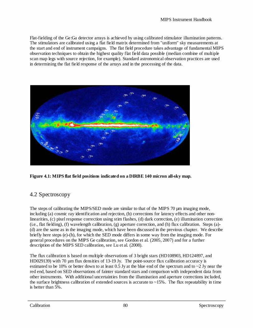
MIPS Instrument Handbook
Calibration 80
Spectroscopy
Flat-fielding of the Ge:Ga detector arrays is achieved by using calibrated stimulator illumination patterns. The stimulators are calibrated using a flat field matrix determined from ''uniform'' sky measurements at the start and end of instrument campaigns. The flat field procedure takes advantage of fundamental MIPS observation techniques to obtain the highest quality flat field data possible (median combine of multiple scan map legs with source rejection, for example). Standard astronomical observation practices are used in determining the flat field response of the arrays and in the processing of the data.
Figure 4.1: MIPS flat field positions indicated on a DIRBE 140 micron all-sky map.
4.2 Spectroscopy
The steps of calibrating the MIPS/SED mode are similar to that of the MIPS 70 µm imaging mode, including (a) cosmic ray identification and rejection, (b) corrections for latency effects and other non-linearities, (c) pixel response correction using stim flashes, (d) dark correction, (e) illumination correction (i.e., flat fielding), (f) wavelength calibration, (g) aperture correction, and (h) flux calibration. Steps (a)-(d) are the same as in the imaging mode, which have been discussed in the previous chapter. We describe briefly here steps (e)-(h), for which the SED mode differs in some way from the imaging mode. For general procedures on the MIPS Ge calibration, see Gordon et al. (2005, 2007) and for a further description of the MIPS SED calibration, see Lu et al. (2008). The flux calibration is based on multiple observations of 3 bright stars (HD108903, HD124897, and HD029139) with 70 µm flux densities of 13-19 Jy. The point-source flux calibration accuracy is estimated to be 10% or better down to at least 0.5 Jy at the blue end of the spectrum and to ~2 Jy near the red end, based on SED observations of fainter standard stars and comparison with independent data from other instruments. With additional uncertainties from the illumination and aperture corrections included, the surface brightness calibration of extended sources is accurate to ~15%. The flux repeatability in time is better than 5%.

MIPS Instrument Handbook
Calibration 81
Spectroscopy
4.2.1 Wavelength
The SED wavelength calibration was obtained on-orbit by observing the planetary nebulae NGC 6543, NGC 6826, and IC 3568. In addition, the supernova remnant IC 443 and the H II region 30 Dor were observed. For all objects, except IC 443, the [O III] 88.3 µm emission line was detected and measured. The [O III] line was the only spectral feature identified in these spectra. For IC 443, the only identified spectral feature was [O I] 63.2 µm. Combining the measurements from these nebulae yields a spectral coverage of 52 µm to 97 µm for SED mode and a dispersion of 1.71 µm/px. There is a shift of less than a pixel in the position of emission lines along the usable length of the slit, and the centroid of the spectrum on the array shifts by about a pixel from the blue to the red end of the spectrum. The dispersion solution was determined by observing a number of bright planetary nebulae and HII regions. The main spectral lines for this purpose are [NIII]57.330µm and [OIII]88.356µm, which have high equivalent widths in these objects. As an example, Figure 4.2 illustrates the observed line profiles of the planetary nebula NGC 6543.
Figure 4.2: An SED spectrum of the bright planetary nebula NGC 6543 from an observation in MIPS Campaign 20. The spectrum is extracted with a 5-column aperture. Both [NIII] 57µm and [OIII] 88µm lines are clearly detected. The measured line peak positions along with the assumption of a uniform dispersion across the entire wavelength range yields to scale of 1.70 µm per pixel. The first row of the array (i.e., the blue end) corresponds to 52.55 µm. Each line fitting uses 4 independent data points, the wavelength calibration uncertainty is estimated to be on the order of 0.4 µm (0.5*1.70µm / sqrt(4)) if the uniform dispersion assumption holds.
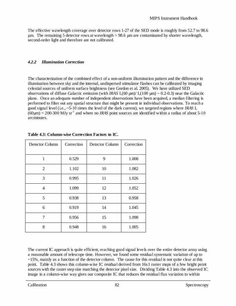
MIPS Instrument Handbook
Calibration 82
Spectroscopy
The effective wavelength coverage over detector rows 1-27 of the SED mode is roughly from 52.7 to 98.6 µm. The remaining 5 detector rows at wavelength > 98.6 µm are contaminated by shorter wavelength, second-order light and therefore are not calibrated.
4.2.2 Illumination Correction
The characterization of the combined effect of a non-uniform illumination pattern and the difference in illumination between sky and the internal, undispersed stimulator flashes can be calibrated by imaging celestial sources of uniform surface brightness (see Gordon et al. 2005). We have utilized SED observations of diffuse Galactic emission (with IRAS Iν(60 µm)/ Iν(100 µm) ~ 0.2-0.3) near the Galactic plane. Once an adequate number of independent observations have been acquired, a median filtering is performed to filter out any spatial structure that might be present in individual observations. To reach a good signal level (i.e., ~5-10 times the level of the dark current), we targeted regions where IRAS Iν (60µm) = 200-300 MJy sr-1 and where no IRAS point sources are identified within a radius of about 5-10 arcminutes.
Table 4.3: Column-wise Correction Factors to IC.
Detector Column Correction
Detector Column Correction
1 0.529 9 1.008
2 1.102 10 1.082
3 0.995 11 1.026
4 1.099 12 1.052
5 0.938 13 0.958
6 0.919 14 1.045
7 0.956 15 1.098
8 0.948 16 1.005
The current IC approach is quite efficient, reaching good signal levels over the entire detector array using a reasonable amount of telescope time. However, we found some residual systematic variation of up to ~15%, mainly as a function of the detector column. The cause for this residual is not quite clear at this point. Table 4.3 shows this column-wise IC residual derived from 16x1 raster maps of a few bright point sources with the raster step size matching the detector pixel size. Dividing Table 4.3 into the observed IC image in a column-wise way gives our composite IC that reduces the residual flux variation to within
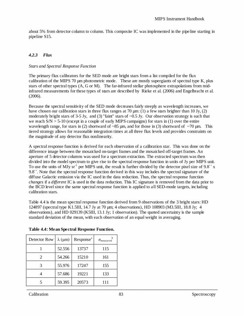
MIPS Instrument Handbook
Calibration 83
Spectroscopy
about 5% from detector column to column. This composite IC was implemented in the pipeline starting in pipeline S15.
4.2.3 Flux
Stars and Spectral Response Function
The primary flux calibrators for the SED mode are bright stars from a list compiled for the flux calibration of the MIPS 70 µm photometric mode. These are mostly supergiants of spectral type K, plus stars of other spectral types (A, G or M). The far-infrared stellar photosphere extrapolations from mid-infrared measurements for these types of stars are described by Rieke et al. (2006) and Engelbracht et al. (2006). Because the spectral sensitivity of the SED mode decreases fairly steeply as wavelength increases, we have chosen our calibration stars in three flux ranges at 70 µm: (1) a few stars brighter than 10 Jy, (2) moderately bright stars of 3-5 Jy, and (3) ''faint'' stars of ~0.5 Jy. Our observation strategy is such that we reach S/N > 5-10 (except in a couple of early MIPS campaigns) for stars in (1) over the entire wavelength range, for stars in (2) shortward of ~85 µm, and for those in (3) shortward of ~70 µm. This tiered strategy allows for reasonable integration times at all three flux levels and provides constraints on the magnitude of any detector flux nonlinearity. A spectral response function is derived for each observation of a calibration star. This was done on the difference image between the mosaicked on-target frames and the mosaicked off-target frames. An aperture of 5 detector columns was used for a spectrum extraction. The extracted spectrum was then divided into the model spectrum to give rise to the spectral response function in units of Jy per MIPS unit. To use the units of MJy sr-1 per MIPS unit, the result is further divided by the detector pixel size of 9.8´ ́x 9.8´ .́ Note that the spectral response function derived in this way includes the spectral signature of the diffuse Galactic emission via the IC used in the data reduction. Thus, the spectral response function changes if a different IC is used in the data reduction. This IC signature is removed from the data prior to the BCD level since the same spectral response function is applied to all SED-mode targets, including calibration stars. Table 4.4 is the mean spectral response function derived from 9 observations of the 3 bright stars: HD 124897 (spectral type K1.5III, 14.7 Jy at 70 µm; 4 observations), HD 108903 (M3.5III, 18.8 Jy; 4 observations), and HD 029139 (K5III, 13.1 Jy; 1 observation). The quoted uncertainty is the sample standard deviation of the mean, with each observation of an equal weight in averaging.
Table 4.4: Mean Spectral Response Function.
Detector Row λ (µm) Responsea σmeasuredb
1 52.556 13737 115
2 54.266 15210 161
3 55.976 17247 155
4 57.686 19221 133
5 59.395 20573 111
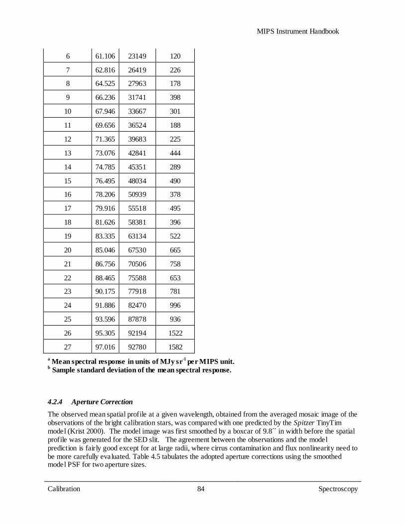
MIPS Instrument Handbook
Calibration 84
Spectroscopy
6 61.106 23149 120
7 62.816 26419 226
8 64.525 27963 178
9 66.236 31741 398
10 67.946 33667 301
11 69.656 36524 188
12 71.365 39683 225
13 73.076 42841 444
14 74.785 45351 289
15 76.495 48034 490
16 78.206 50939 378
17 79.916 55518 495
18 81.626 58381 396
19 83.335 63134 522
20 85.046 67530 665
21 86.756 70506 758
22 88.465 75588 653
23 90.175 77918 781
24 91.886 82470 996
25 93.596 87878 936
26 95.305 92194 1522
27 97.016 92780 1582 a Mean spectral response in units of MJy sr-1 per MIPS unit. b Sample standard deviation of the mean spectral response.
4.2.4 Aperture Correction
The observed mean spatial profile at a given wavelength, obtained from the averaged mosaic image of the observations of the bright calibration stars, was compared with one predicted by the Spitzer TinyTim model (Krist 2000). The model image was first smoothed by a boxcar of 9.8´́ in width before the spatial profile was generated for the SED slit. The agreement between the observations and the model prediction is fairly good except for at large radii, where cirrus contamination and flux nonlinearity need to be more carefully evaluated. Table 4.5 tabulates the adopted aperture corrections using the smoothed model PSF for two aperture sizes.
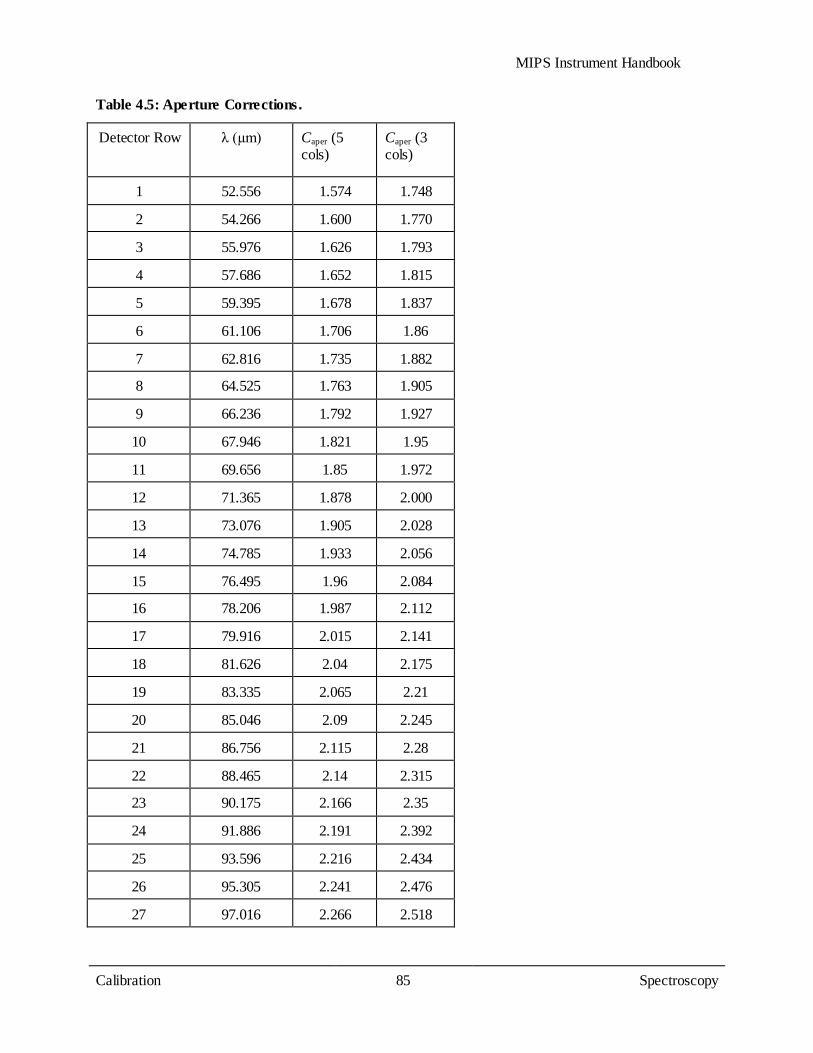
MIPS Instrument Handbook
Calibration 85
Spectroscopy
Table 4.5: Aperture Corrections.
Detector Row λ (µm) Caper (5 cols)
Caper (3 cols)
1 52.556 1.574 1.748
2 54.266 1.600 1.770
3 55.976 1.626 1.793
4 57.686 1.652 1.815
5 59.395 1.678 1.837
6 61.106 1.706 1.86
7 62.816 1.735 1.882
8 64.525 1.763 1.905
9 66.236 1.792 1.927
10 67.946 1.821 1.95
11 69.656 1.85 1.972
12 71.365 1.878 2.000
13 73.076 1.905 2.028
14 74.785 1.933 2.056
15 76.495 1.96 2.084
16 78.206 1.987 2.112
17 79.916 2.015 2.141
18 81.626 2.04 2.175
19 83.335 2.065 2.21
20 85.046 2.09 2.245
21 86.756 2.115 2.28
22 88.465 2.14 2.315
23 90.175 2.166 2.35
24 91.886 2.191 2.392
25 93.596 2.216 2.434
26 95.305 2.241 2.476
27 97.016 2.266 2.518

MIPS Instrument Handbook
Calibration 86
Spectroscopy
Comparison with Models and Previous Observations
An empirical way to derive an absolute calibration accuracy is to compare SED measured fluxes with the model predicted values for stars not used in the derivation of the spectral response function. This is shown in Figure 4.3 at three representative wavelengths: 60, 71.4 and 80 µm. From these data, it is reasonable to conclude that a flux accuracy better than 10% is achieved down to a flux density of ~0.5 Jy at the blue end of the spectra, or a couple of Janskys near the red end. This empirical accuracy estimate includes uncertainties in the stellar model fluxes. In Figure 4.3 the faint stars apparently have a lower spectral response than the bright stars. This is most noticeable at 60 µm (see Figure 4.3a), at which the difference is on the order of 5-7% over the 70 µm flux range of 0.5-18 Jy. It is plausible that part of this apparent flux dependency can be attributed to the flux nonlinearity. A number of calibration stars have been observed in multiple campaigns. These include stars of all three flux levels (cf. Figure 4.3). The results indicate a fairly high flux repeatability in time: the r.m.s. difference goes from ~2% near the blue end of the spectrograph to better than 5% near the red end. Figure 4.4 compares MIPS/SED fluxes with IRAS 60 and 100 µm fluxes for the galaxy NGC 4418, and with ISO LWS data for the galaxy Mrk 231. The results from these cross-comparison analyses are all consistent with that the absolute flux calibration of the SED mode is accurate to 10% or better for point sources.
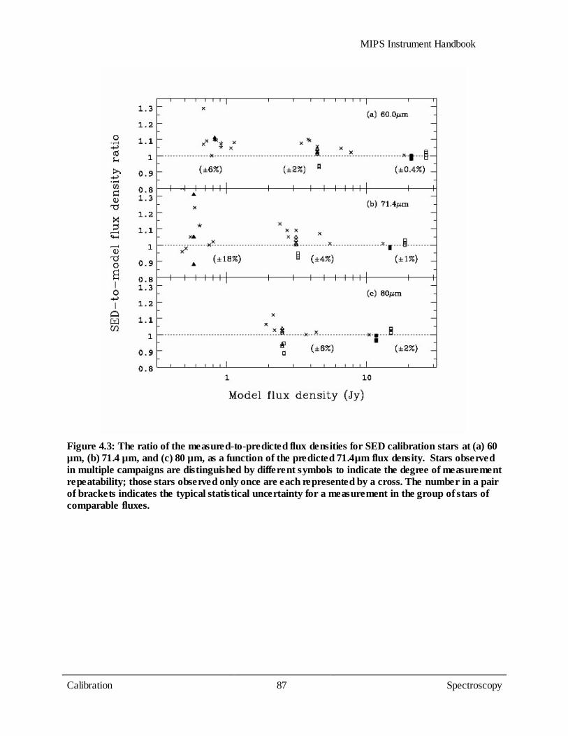
MIPS Instrument Handbook
Calibration 87
Spectroscopy
Figure 4.3: The ratio of the measured-to-predicted flux densities for SED calibration stars at (a) 60 µm, (b) 71.4 µm, and (c) 80 µm, as a function of the predicted 71.4µm flux density. Stars observed in multiple campaigns are distinguished by different symbols to indicate the degree of measurement repeatability; those stars observed only once are each represented by a cross. The number in a pair of brackets indicates the typical statistical uncertainty for a measurement in the group of stars of comparable fluxes.
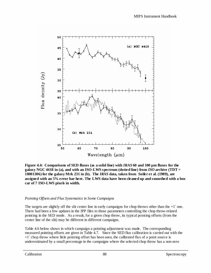
MIPS Instrument Handbook
Calibration 88
Spectroscopy
Figure 4.4: Comparisons of SED fluxes (as a solid line) with IRAS 60 and 100 µm fluxes for the galaxy NGC 4418 in (a), and with an ISO-LWS spectrum (dotted line) from ISO archive (TDT = 18001306) for the galaxy Mrk 231 in (b). The IRAS data, taken from Soifer et al. (1989), are assigned with an 5% error bar here. The LWS data have been cleaned up and smoothed with a box car of 7 ISO-LWS pixels in width.
Pointing Offsets and Flux Systematics in Some Campaigns
The targets are slightly off the slit center line in early campaigns for chop throws other than the +1 ́one. There had been a few updates in the IPP files to those parameters controlling the chop throw-related pointing in the SED mode. As a result, for a given chop throw, its typical pointing offsets (from the center line of the slit) may be different in different campaigns. Table 4.6 below shows in which campaign a pointing adjustment was made. The corresponding measured pointing offsets are given in Table 4.7. Since the SED flux calibration is carried out with the +1 ́chop throw where little pointing offset has been seen, the calibrated flux of a point source is underestimated by a small percentage in the campaigns where the selected chop throw has a non-zero
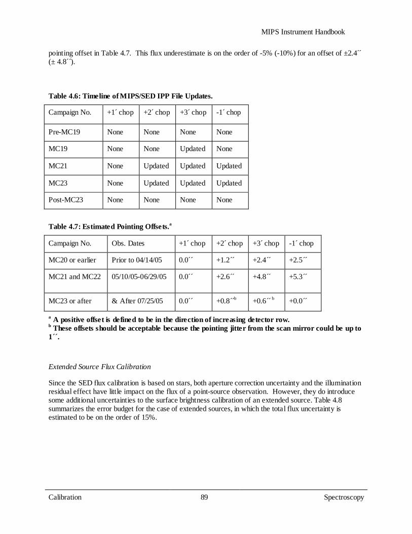
MIPS Instrument Handbook
Calibration 89
Spectroscopy
pointing offset in Table 4.7. This flux underestimate is on the order of -5% (-10%) for an offset of ±2.4´́ (± 4.8´ )́.
Table 4.6: Timeline of MIPS/SED IPP File Updates.
Campaign No. +1 ́chop +2 ́chop +3 ́chop -1 ́chop
Pre-MC19 None None None None
MC19 None None Updated None
MC21 None Updated Updated Updated
MC23 None Updated Updated Updated
Post-MC23 None None None None
Table 4.7: Estimated Pointing Offsets.a
Campaign No. Obs. Dates +1 ́chop +2 ́chop +3 ́chop -1 ́chop
MC20 or earlier Prior to 04/14/05 0.0´ ́ +1.2´́ +2.4´́ +2.5´́
MC21 and MC22 05/10/05-06/29/05 0.0´ ́ +2.6´́
+4.8´́ +5.3´́
MC23 or after & After 07/25/05 0.0´ ́ +0.8´́ b +0.6´́ b +0.0´́
a A positive offset is defined to be in the direction of increasing detector row. b These offsets should be acceptable because the pointing jitter from the scan mirror could be up to 1´´.
Extended Source Flux Calibration
Since the SED flux calibration is based on stars, both aperture correction uncertainty and the illumination residual effect have little impact on the flux of a point-source observation. However, they do introduce some additional uncertainties to the surface brightness calibration of an extended source. Table 4.8 summarizes the error budget for the case of extended sources, in which the total flux uncertainty is estimated to be on the order of 15%.

MIPS Instrument Handbook
Calibration 90
Basic toolset for working with MIPS data
Table 4.8: Error Budget for Flux Calibration of Extended Sources.
Error Source Estimated Error
Point-source flux uncertainty <= 10%
IC uncertainty after columnwise correction ~5%
Aperture correction uncertainty <= 10%
Total ~15%
Remarks on Flux Nonlinearity
MIPS Ge detector flux nonlinearity is addressed using calibration data taken in the 70 µm imaging mode, which is more sensitive than the SED mode. No significant (i.e., < 10%) flux nonlinearity is seen in the SED mode over a flux range of 0.5 to ~40 Jy at 70 µm. However, for a flux far outside this range, the flux nonlinearity could be increasingly important. Without a proper correction for it, the systematic effect from a flux nonlinearity would be an underestimate (overestimate) of the real flux of a very bright (faint) source.
4.3 Basic toolset for working with MIPS data
MIPS data are produced as standard FITS files, appropriate for use in IRAF, IDL, or your own favorite image analysis software. HOWEVER, Spitzer images are in units of surface brightness, MJy/sr, which may be unfamiliar to observers coming from other wavelength regimes. The main implication is that photometry as performed using the same routines used for, e.g., optical data may not return the correct values. Section 4.3.1 covers these items. Color corrections may be important for some observers; see section 4.3.4. Observers doing aperture photometry will want to make aperture corrections, and, on a related front, observers doing PSF fitting may be interested in the PSF shape itself; section 4.3.6 discusses the PSF.
4.3.1 Units and flux densities
MIPS images are in MJy/sr. (To convert from MJy/sr to microJy/arcsecond2, multiply by 23.5045.) When summing up the flux incident on a set of pixels for, e.g., aperture photometry, you need to multiply by the number of steradian per pixel. See Table 4.9 for average actual pixel sizes; see the BCD header values of PXSCAL1 and PXSCAL2 in your own data for values specific to your program because the pixel scale changes slightly as a function of mirror position. Note that these values may be refined as our knowledge of the instrument matures. One square arcsecond is 2.3504x10⁻¹¹ steradian. Note that post-BCD products are resampled images such that the pixels have different sizes from the pixels in the original BCDs. Please check the post-BCD header keywords CDELT1 and CDELT2 for the
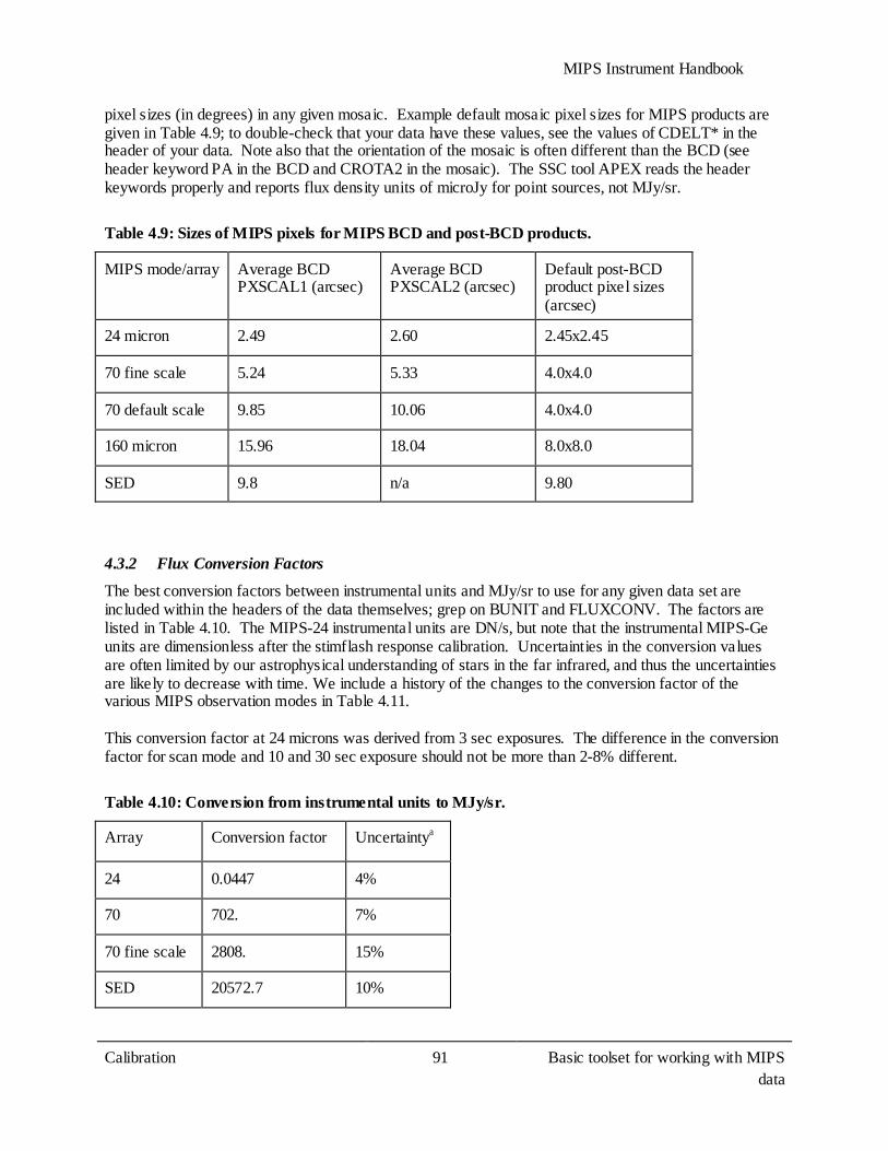
MIPS Instrument Handbook
Calibration 91
Basic toolset for working with MIPS data
pixel sizes (in degrees) in any given mosaic. Example default mosaic pixel sizes for MIPS products are given in Table 4.9; to double-check that your data have these values, see the values of CDELT* in the header of your data. Note also that the orientation of the mosaic is often different than the BCD (see header keyword PA in the BCD and CROTA2 in the mosaic). The SSC tool APEX reads the header keywords properly and reports flux density units of microJy for point sources, not MJy/sr.
Table 4.9: Sizes of MIPS pixels for MIPS BCD and post-BCD products.
MIPS mode/array Average BCD PXSCAL1 (arcsec)
Average BCD PXSCAL2 (arcsec)
Default post-BCD product pixel sizes (arcsec)
24 micron 2.49 2.60 2.45x2.45
70 fine scale 5.24 5.33 4.0x4.0
70 default scale 9.85 10.06 4.0x4.0
160 micron 15.96 18.04 8.0x8.0
SED 9.8 n/a 9.80
4.3.2 Flux Conversion Factors
The best conversion factors between instrumental units and MJy/sr to use for any given data set are included within the headers of the data themselves; grep on BUNIT and FLUXCONV. The factors are listed in Table 4.10. The MIPS-24 instrumental units are DN/s, but note that the instrumental MIPS-Ge units are dimensionless after the stimflash response calibration. Uncertainties in the conversion values are often limited by our astrophysical understanding of stars in the far infrared, and thus the uncertainties are likely to decrease with time. We include a history of the changes to the conversion factor of the various MIPS observation modes in Table 4.11. This conversion factor at 24 microns was derived from 3 sec exposures. The difference in the conversion factor for scan mode and 10 and 30 sec exposure should not be more than 2-8% different.
Table 4.10: Conversion from instrumental units to MJy/sr.
Array Conversion factor Uncertaintya
24 0.0447 4%
70 702. 7%
70 fine scale 2808. 15%
SED 20572.7 10%

MIPS Instrument Handbook
Calibration 92
Basic toolset for working with MIPS data
160 41.7 12%
a For optimal data reduction and flux density extraction of single sources in photometric mode, the uncertainties can be as small as 2%/5%/10% for 24/70/70fine.
Table 4.11: Changes in Conversion Factor with Pipeline.
Pipeline Versiona
24 µm 70 µm 70 µm Fine
70 µm SED 160 µm
S10 0.04391 634. --- --- 42
S11 0.04391 634. 2536. 27093 42
S12 0.04391 634. 2536. 21835 42
S13 0.04391 702. 2808. 20572.7 44.7
S16 0.0447 702. 2808. 20572.7 44.7
S17 0.0447 702. 2808. 20572.7 41.7
a This history is meant to be suggestive of what changes occurred and when. The process of pipeline updates was complicated, with multiple versions and versions that were replaced before significant data was run through them. The data header will always contain the correct conversion factor used.
4.3.3 Magnitude Zero Points
Dr. C. Engelbracht has computed MIPS magnitude zero points using the Kurucz (1993) Vega model, which has then been scaled to the Rieke et al. (2008) 10.6µm zero point of 35.03 ± 0.3 Jy. He has further assumed that Vega is 0 magnitudes in all MIPS bands, and has computed fluxes at 23.68, 71.42, and 155.9 µm. The resultant zero points are in Table 4.12.
Table 4.12: Magnitude zero points.
Wavelength (microns) Zero point (Jy) Uncertainty (Jy)
23.68 7.17 0.11
71.42 0.778 0.012
155.9 0.159 0.020

MIPS Instrument Handbook
Calibration 93
Basic toolset for working with MIPS data
4.3.4 Aperture Correction
For aperture corrections, you should also consider constructing your own PSF from your own data, because aperture corrections may vary for different source colors . In Figure 4.5, there is a source of 0.5 Jy from the Extragalactic First-Look Survey (XFLS) main field (at 17:23:44.1 +59:05:18, J2000); there are three radii (1.35, 2, 3 times the FWHM, 5.9 arcsec) in white; the black circle is a 100 arcsec radius. Figure 4.6 shows the ''curve of growth'' to indicate the fraction of the total flux enclosed by smaller apertures. The Instrument Support Team (IST) at the SSC and the Instrument Team (IT) at the University of Arizona as part of a large project to better understand and to improve the MIPS photometric calibration, have determined different aperture corrections for the current MIPS Photometric modes (24 um, 70 um, 70 um fine scale and 160 um) plus Spectral Energy Distribution (SED). The tables below (Table 4.13, Table 4.14, and Table 4.15) summarize these efforts. These example corrections should be good to ~5%, but we emphasize again the importance of deriving this yourself for your own targets and data. Even if you don t́ have enough point sources in your own data to generate your very own PSF, we strongly suggest deriving your own aperture corrections using the copious public data or STINYTIM, or the observed PSFs provided on the web.
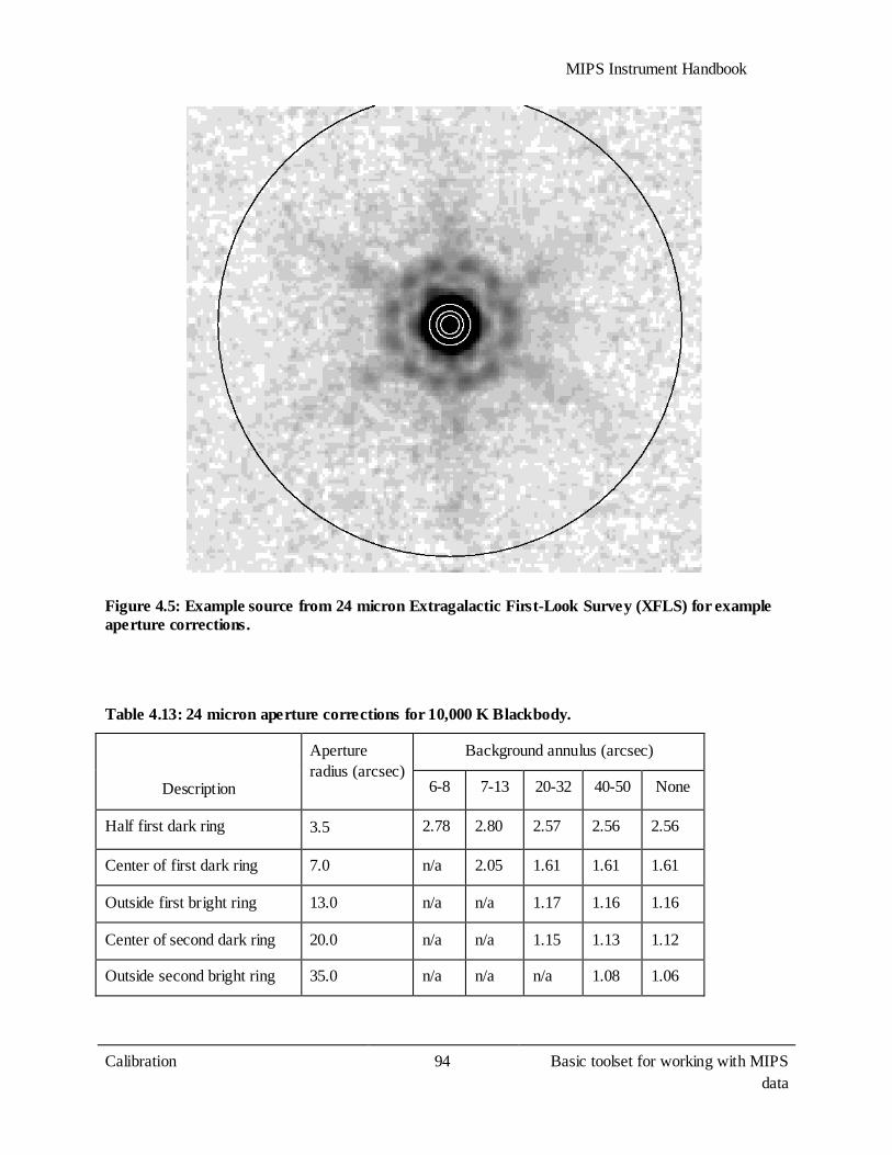
MIPS Instrument Handbook
Calibration 94
Basic toolset for working with MIPS data
Figure 4.5: Example source from 24 micron Extragalactic First-Look Survey (XFLS) for example aperture corrections.
Table 4.13: 24 micron aperture corrections for 10,000 K Blackbody.
Description
Aperture radius (arcsec)
Background annulus (arcsec)
6-8 7-13 20-32 40-50 None
Half first dark ring 3.5 2.78 2.80 2.57 2.56 2.56
Center of first dark ring 7.0 n/a 2.05 1.61 1.61 1.61
Outside first bright ring 13.0 n/a n/a 1.17 1.16 1.16
Center of second dark ring 20.0 n/a n/a 1.15 1.13 1.12
Outside second bright ring 35.0 n/a n/a n/a 1.08 1.06
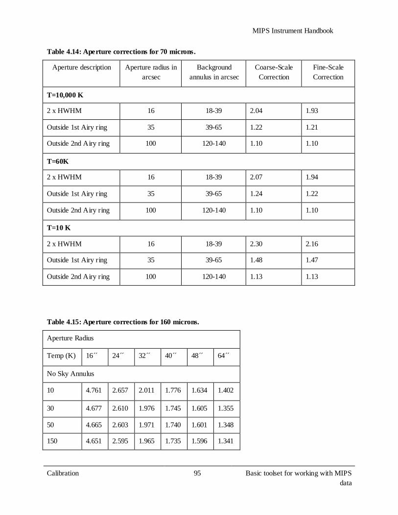
MIPS Instrument Handbook
Calibration 95
Basic toolset for working with MIPS data
Table 4.14: Aperture corrections for 70 microns.
Aperture description Aperture radius in arcsec
Background annulus in arcsec
Coarse-Scale Correction
Fine-Scale Correction
T=10,000 K
2 x HWHM 16 18-39 2.04 1.93
Outside 1st Airy ring 35 39-65 1.22 1.21
Outside 2nd Airy ring 100 120-140 1.10 1.10
T=60K
2 x HWHM 16 18-39 2.07 1.94
Outside 1st Airy ring 35 39-65 1.24 1.22
Outside 2nd Airy ring 100 120-140 1.10 1.10
T=10 K
2 x HWHM 16 18-39 2.30 2.16
Outside 1st Airy ring 35 39-65 1.48 1.47
Outside 2nd Airy ring 100 120-140 1.13 1.13
Table 4.15: Aperture corrections for 160 microns.
Aperture Radius
Temp (K) 16´́ 24´́ 32´́ 40´́ 48´́ 64´́
No Sky Annulus
10 4.761 2.657 2.011 1.776 1.634 1.402
30 4.677 2.610 1.976 1.745 1.605 1.355
50 4.665 2.603 1.971 1.740 1.601 1.348
150 4.651 2.595 1.965 1.735 1.596 1.341
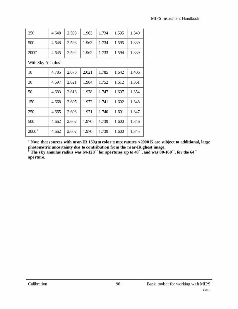
MIPS Instrument Handbook
Calibration 96
Basic toolset for working with MIPS data
250 4.648 2.593 1.963 1.734 1.595 1.340
500 4.648 2.593 1.963 1.734 1.595 1.339
2000a 4.645 2.592 1.962 1.733 1.594 1.339
With Sky Annulusb
10 4.785 2.670 2.021 1.785 1.642 1.406
30 4.697 2.621 1.984 1.752 1.612 1.361
50 4.683 2.613 1.978 1.747 1.607 1.354
150 4.668 2.605 1.972 1.741 1.602 1.348
250 4.665 2.603 1.971 1.740 1.601 1.347
500 4.662 2.602 1.970 1.739 1.600 1.346
2000 a 4.662 2.602 1.970 1.739 1.600 1.345
a Note that sources with near-IR 160µm color temperatures >2000 K are subject to additional, large photometric uncertainty due to contribution from the near-IR ghost image. b The sky annulus radius was 64-128´ ́for apertures up to 48´´, and was 80-160´´, for the 64´ ́aperture.
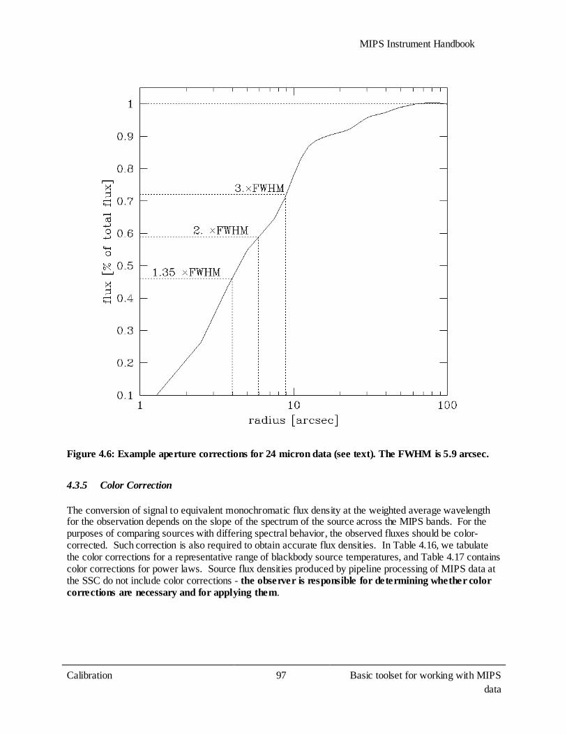
MIPS Instrument Handbook
Calibration 97
Basic toolset for working with MIPS data
Figure 4.6: Example aperture corrections for 24 micron data (see text). The FWHM is 5.9 arcsec.
4.3.5 Color Correction
The conversion of signal to equivalent monochromatic flux density at the weighted average wavelength for the observation depends on the slope of the spectrum of the source across the MIPS bands. For the purposes of comparing sources with differing spectral behavior, the observed fluxes should be color-corrected. Such correction is also required to obtain accurate flux densities. In Table 4.16, we tabulate the color corrections for a representative range of blackbody source temperatures, and Table 4.17 contains color corrections for power laws. Source flux densities produced by pipeline processing of MIPS data at the SSC do not include color corrections - the observer is responsible for determining whether color corrections are necessary and for applying them.

MIPS Instrument Handbook
Calibration 98
Basic toolset for working with MIPS data
Table 4.16: Nominal color corrections vs. blackbody source temperature.
Lambda (µm)
Source Temperature (K)
104 5000 1000 500 300 200 150 100 70 50 30 20
23.68 1.000 0.999 0.992 0.983 0.970 0.957 0.948 0.947 0.986 1.119 2.031 7.005
71.42 1.000 0.999 0.995 0.989 0.980 0.970 0.959 0.938 0.914 0.893 0.901 1.052
155.9 1.000 1.000 0.999 0.997 0.996 0.993 0.991 0.986 0.979 0.971 0.954 0.944
Table 4.17: Nominal color corrections for power laws.
Power law indices (alpha) where
Lambda (µm)
-3 -2 -1 0 1 2 3
23.68 0.967 0.960 0.961 0.967 0.981 1.001 1.027
71.42 0.933 0.918 0.918 0.932 0.959 1.001 1.057
155.9 0.965 0.959 0.959 0.965 0.979 1.000 1.029
The flux of a source is typically determined relative to calibrator stars using the ratio of the stellar and source signals. The nominal flux derived in this manner must be corrected in order to derive the true monochromatic flux density at the weighted average wavelength for the band by dividing by the appropriate factor in Table 4.16. The result will be the 'best estimate' of the true monochromatic flux density of the unknown source at the weighted average wavelength. The photometric bandwidths of the MIPS filters were selected to make these corrections modest, except for sources whose blackbody spectral energy distributions peak at wavelengths longer than the photometric band. In these cases, large corrections are unavoidable; observers measuring cold objects should take note. Note that MIPS and IRAC calculate color corrections slightly differently; the origin of this difference is that our response functions are in slightly different units. As such, to reproduce the color corrections displayed here, you will need to do the following. Take the response functions from the website (units of electrons per unit energy) and divide by lambda (to get electrons per photon). MIPS defines λ 0 as follows:
(4.1)

MIPS Instrument Handbook
Calibration 99
Basic toolset for working with MIPS data
where Rλ is the response function in units of electrons per photon. MIPS color corrections are referenced to a 10,000 K blackbody:
(4.2)
where : T0=10,000 K, λ0
=23.675 microns at MIPS-24,
λ0=71.440 microns at MIPS-70,
λ0=155.899 microns at MIPS-160, and
hc/k = 14388 microns x K For an input blackbody at Teff, the numerator of equation 4.2 becomes:
(4.3)
and for power laws, the numerator becomes (alpha=2 for the Rayleigh-Jeans limit):
(4.4)
Users should DIVIDE by the color-corrections (K) given in Table 4.16 and Table 4.17 to convert the observed flux densities to real flux densities.
4.3.6 PSF Characterization
Characterizing MIPS PSFs can be difficult because MIPS has five different observing modes, large arrays (distortion!), multiple mirror positions in each mode (distortion!), and large bandpasses (color terms!). The STINYTIM software simulation of the PSFs actually matches our observed PSF quite well, as the optics are very smooth at these long wavelengths. One way in which there is a significant difference is the short-wavelength light leak at 160 microns; for more information on this, see section 7.2.6 below. Note
MIPS Instrument Handbook
Calibration 100
Basic toolset for working with MIPS data
that the STINYTIM simulation PSFs are oversampled, and the pixel sizes do not match what you actually get with default Spitzer data. In general, if you need to do a detailed PSF subtraction, we recommend that you create one from your own data (using objects of similar color to your target) to ensure that you have PSF standards of the same color and brightness and observed with exactly the same AOR parameters. The lack of repeatability in scan mirror position from campaign to campaign makes it necessary to do the PSF observation in the same campaign as the science observation. The Archive does not maintain a library of PSFs with characteristics spanning the full range of observer needs for PSF subtraction. The point response function (PRF) is a similar but distinct concept from that of the PSF. Where the PSF is the point spread function before sampling by the detector array, the PRF gives the relative pixel values coming out of the array. The PRF is essentially a convolution of a box the size of the image pixel with the PSF. The software package APEX uses PRFs to carry out point source extraction. More detailed documentation on APEX can be found in the Data Analysis section of the website. There are various ways to create PRFs to carry out point source extraction with APEX. For a single frame source extraction with APEX, e.g. extraction from a MOSAIC, the PRF is slightly different from that one used in single BCDs. There are PRFs posted on the MIPS portion of the website that have been created from BCDs, from mosaics, and from STINYTIM. These PRFs are based on the SSC mosaic pixel scale: 2.45 arcsec/pix and resampled by a factor of 4. Users should keep in mind that different mosaic pixel scales and/or resampling factors produce different PRFs. The empirical PRFs were created using PRF_ESTIMATE (from the MOPEX package), which is a script that combines those stars selected by the user, from a post-BCD mosaic, into a ''mosaic PRF''. Usually these stars have a high signal-to-noise and no neighbors, i.e. they are the best and cleanest for the job. How different is the empirical PRF compared with the one derived using STINYTIM? They are not that different, but they are not identical. The main difference is at the depth of the first Airy ring, which is deeper in the STINYTIM PRF. Please note: There is not a ''magic PRF'' that will work for every data set.
4.3.7 Astrometry - Including Distortion and Pointing
Absolute pointing knowledge of the focal plane array pixel centers based on the Pointing Control System is better than:
• 24 µm : about 1.4´´, 1 sigma radial • 70 µm : about 1.7´´, 1 sigma radial • 160 µm : about 3.9´´, 1 sigma radial
From the science data frames themselves, refined pointing knowledge of sources must be based on centroiding of objects visible in a MIPS image. The uncertainties will depend on the signal-to-noise ratio of those source detections and the related uncertainty in the centroids, and on the accuracy of prior knowledge of the positions of some or all of the sources. Uncertainty in relative positions between sources (source offsets) can be much lower than those associated with absolute pointing knowledge, for detections that can support this type of analysis.
MIPS Instrument Handbook
Calibration 101
Start-Up and Shut-Down Procedures
The pointing offsets used in mapping of individual frames into the post-BCD products are derived from an optimal offset estimation method, e.g., point source extraction. If insufficient point sources are available, then the data are aligned using spacecraft and CSMM pointing knowledge only. Individual frames are adjusted such that the overlap regions are statistically similar, within the limitations of the large-scale background and slow response characteristics of the Ge:Ga detectors. This implies that some edges might be visible for certain types of varying backgrounds. This will especially be true for adjacent legs of a scan map over a region with significant and varying background. The absolute level to which edge effects and scan leg baseline offsets will be removed in the post-BCD products will not be known with certainty until more flight data are obtained. For observers requiring very uniform maps of extended source regions, there should be some expectation of additional required data processing to correct for edge effects and scan leg baseline offsets in the Ge:Ga data of a scan map. Such effects are minimized in the other MIPS observing modes. The zodiacal backgrounds are maintained only within an individual AOR.
4.4 Start-Up and Shut-Down Procedures
Sets of basic data for determining the absolute calibration of the detectors were obtained at the beginning and end of each MIPS instrument campaign. Various types of well-studied astronomical sources are observed for this purpose (see section 4.1.2). These observations did not need to be taken more frequently because of the stability of the stimulator output over time, and the exhaustive use of stimulator flashes built-in to all MIPS observing templates. To keep the observatory observation efficiency at a maximum, ''unnecessary'' calibration data acquisition was avoided. Because there is contamination on the pick-off mirror that feeds MIPS (see section 7.1.1), each campaign included sets of scan-mirror-position-dependent flat fields for the 24 µm array.
Start-up Sequence
• If not already on for IRS, switch on the Combined Electronics and other MIPS electronics requiring specific turn-on commanding.
• After the required warm-up time (0.5 hour), proceed with routine calibration measurements. • Obtain Ge:Ga detector bias calibration observations • Slew to MIPS ''dark sky'' region. • Thermal anneal all detector arrays. • Acquire dark current data frames for all arrays. • Slew to MIPS ''flat sky'' and acquire flat field frames to provide average uniform illumination. • Acquire flat field projector and stimulator data for the flat field matrix. • Slew to Observatory cross-calibration flux standard(s) for 24 µm. Observe using the Photometry
AOT. • Slew to MIPS 24 µm flux standard(s) (if different from above) and observe using the Photometry
AOT. • Slew to MIPS 70 µm flux standard(s) and observe using the Photometry AOT. • Slew to MIPS SED flux standards(s) and observe using the SED AOT; also obtain an
illumination correction. • If not a MIPS-warm campaign, slew to MIPS 160 µm flux standard(s) and observe using the
Photometry AOT. • Proceed with science observations as planned for the instrument campaign.

MIPS Instrument Handbook
Calibration 102
Start-Up and Shut-Down Procedures
Shut-down Sequence
• End science observations at the scheduled time. • Slew to MIPS ''dark sky'' region. • Thermal anneal all detector arrays. • Acquire dark current data frames for all arrays. • Slew to Observatory cross calibration flux standard(s) for 24 µm. Observe using the Photometry
AOT. • Slew to MIPS 24 µm flux standard(s) and observe using the Photometry AOT. • Slew to MIPS 70 µm flux standard(s) and observe using the Photometry AOT. • Slew to MIPS SED flux standards(s) and observe using the SED AOT; also obtain an
illumination correction. • If not a MIPS-warm campaign, slew to MIPS 160 µm flux standard(s) and observe using the
Photometry AOT. • Obtain Ge:Ga detector bias calibration observations. • If not required by IRS, switch off the Combined Electronics and other MIPS electronics requiring
specific turn-off commanding.
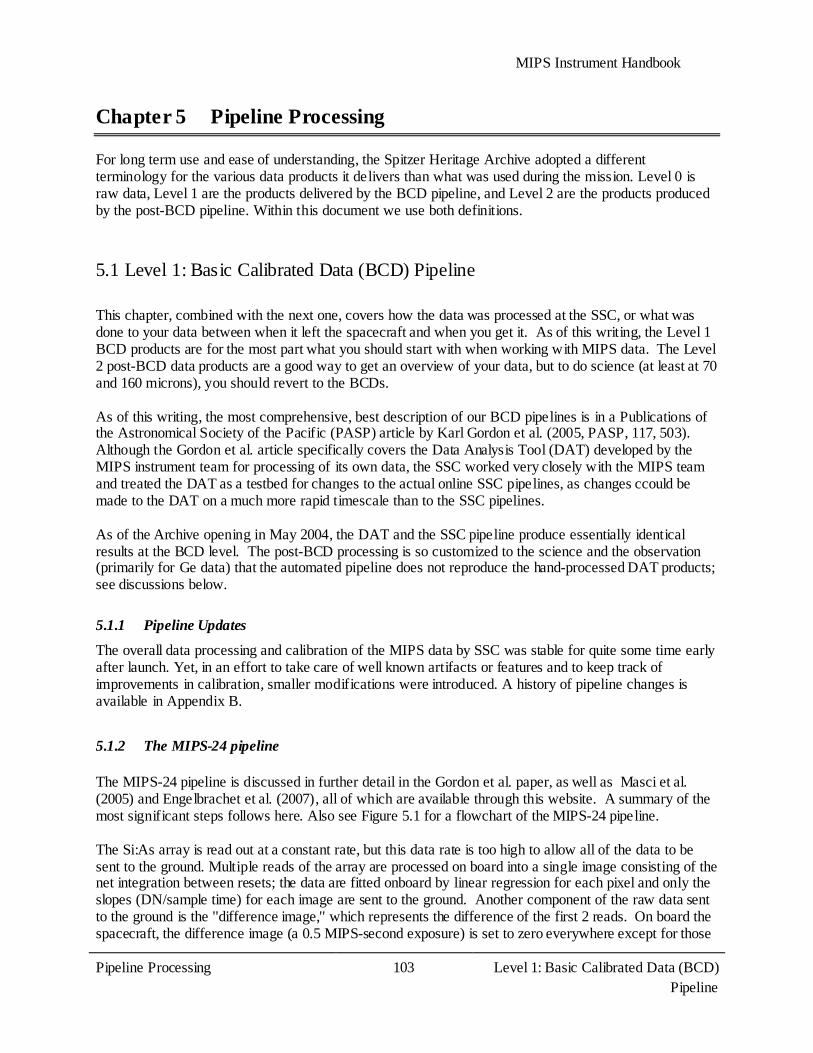
MIPS Instrument Handbook
Pipeline Processing 103
Level 1: Basic Calibrated Data (BCD) Pipeline
Chapter 5 Pipeline Processing
For long term use and ease of understanding, the Spitzer Heritage Archive adopted a different terminology for the various data products it delivers than what was used during the mission. Level 0 is raw data, Level 1 are the products delivered by the BCD pipeline, and Level 2 are the products produced by the post-BCD pipeline. Within this document we use both definitions.
5.1 Level 1: Basic Calibrated Data (BCD) Pipeline
This chapter, combined with the next one, covers how the data was processed at the SSC, or what was done to your data between when it left the spacecraft and when you get it. As of this writing, the Level 1 BCD products are for the most part what you should start with when working with MIPS data. The Level 2 post-BCD data products are a good way to get an overview of your data, but to do science (at least at 70 and 160 microns), you should revert to the BCDs. As of this writing, the most comprehensive, best description of our BCD pipelines is in a Publications of the Astronomical Society of the Pacific (PASP) article by Karl Gordon et al. (2005, PASP, 117, 503). Although the Gordon et al. article specifically covers the Data Analysis Tool (DAT) developed by the MIPS instrument team for processing of its own data, the SSC worked very closely with the MIPS team and treated the DAT as a testbed for changes to the actual online SSC pipelines, as changes ccould be made to the DAT on a much more rapid timescale than to the SSC pipelines. As of the Archive opening in May 2004, the DAT and the SSC pipeline produce essentially identical results at the BCD level. The post-BCD processing is so customized to the science and the observation (primarily for Ge data) that the automated pipeline does not reproduce the hand-processed DAT products; see discussions below.
5.1.1 Pipeline Updates
The overall data processing and calibration of the MIPS data by SSC was stable for quite some time early after launch. Yet, in an effort to take care of well known artifacts or features and to keep track of improvements in calibration, smaller modifications were introduced. A history of pipeline changes is available in Appendix B.
5.1.2 The MIPS-24 pipeline
The MIPS-24 pipeline is discussed in further detail in the Gordon et al. paper, as well as Masci et al. (2005) and Engelbrachet et al. (2007), all of which are available through this website. A summary of the most significant steps follows here. Also see Figure 5.1 for a flowchart of the MIPS-24 pipeline. The Si:As array is read out at a constant rate, but this data rate is too high to allow all of the data to be sent to the ground. Multiple reads of the array are processed on board into a single image consisting of the net integration between resets; the data are fitted onboard by linear regression for each pixel and only the slopes (DN/sample time) for each image are sent to the ground. Another component of the raw data sent to the ground is the ''difference image,'' which represents the difference of the first 2 reads. On board the spacecraft, the difference image (a 0.5 MIPS-second exposure) is set to zero everywhere except for those

MIPS Instrument Handbook
Pipeline Processing 104
Level 1: Basic Calibrated Data (BCD) Pipeline
pixels whose count rate is large enough to lead to an A-to-D (analog to digital) saturation in the data ramp over the total image integration. This is performed on-board using a nominal (and conservative) difference threshold value of 600 DN/sample time (where one sample time = 0.5 MIPS second = 0.524288 real seconds) over a 30 MIPS second integration, or equivalently, ~50.3 MJy/sr. Later in pipeline processing, a larger difference image saturation threshold is used, ~63 MJy/sr. Above this level, the slope pixels are replaced with difference pixels. In the end, this yields more reliable fluxes for bright sources. More specifically, the pipeline re-scales this nominal threshold according to the image integration time since a shorter integration can tolerate a larger count rate before the ramp starts to saturate, and hence bias the slope value. The following scaling is used:
Difference_Sat_Threshold = 1907.34 x (30/EXPTIME) x 0.0447 [MJy/sr] (5.1)
where the factor of 1907.34 is (1000/0.524288]) DN/real seconds, i.e., the nominal threshold for a 30 MIPS second integration, EXPTIME is the image integration time in MIPS seconds, and the factor of 0.0447 is the conversion factor from DN/real seconds to MJy/sr. Of course, some sources may saturate the ramp even in the first read, leading to what's called ''hard saturation'' and then causing the difference value to be zero. The latter cannot be corrected, and the sources will appear to have ''holes'' where sources saturate (usually in the centers of the PSFs) after processing. Also, as the difference pixels approach complete saturation, the signal will drop before becoming zero, so the central holes of hard saturation will be surrounded by pixels of decreasing or even negative slope. After conversion to floating point and DN/sec, the first step is the ''read-2 correction.'' An offset in the second read of the 24-micron array causes the SUR (sample-up-the-ramp) slope to be too large. This effect, referred to in shorthand as ''the read-2 effect,'' results in a gradient across the array that depends on the array position and background level. The correction, which is very small (<<1%), is applied in the regular MIPS pipeline as an analytic function subtracted from SUR slope values. The Si array suffers from the ''droop effect'' whereby the output for a pixel is proportional to the photon signal that fell on that pixel plus a signal proportional to the average signal falling over the entire array. (Also see IRS Instrument Handbook for more discussion of ''droop.'') Because saturated pixels will cause the droop to be underestimated, pixels are first ''desaturated'' using the nonlinearity model and the difference image before the droop correction is calculated. Droop correction is then applied, followed by dark subtraction, nonlinearity correction, flat field division (using mirror position-dependent flat fields), and conversion to units of MJy/sr. Finally, suspected saturated pixels are replaced by those from the first difference image to create reliable slope data wherever possible, resulting in a larger dynamic range. Latent images and potential radhits (cosmic rays) are flagged but not removed at the BCD level. The post-bcd mosaic software is effective in removing radhits from the mosaics (see section 5.2.2). Starting in S18.12 (the final reprocessing data version for the cryogenic Spitzer mission), the Enhanced BCD (EBCD) pipeline was introduced for MIPS-24 photometry mode. Scan mode remains the same as in previous software versions. The EBCD products generally have improved flat fielding, especially with regard to removing spot residuals (see section 6.3.4, Figure 6.4, and Figure 6.5). Occasionally, the EBCD pipeline will not find a good spot match, but in general, there is a great improvement over previous data products. Parallel data (taken when MIPS-70 or MIPS-160 were the primary arrays) also have improved flat fielding, especially for the 160 Enhanced mode, which had no spot correction previous to S18.12 (see

MIPS Instrument Handbook
Pipeline Processing 105
Level 1: Basic Calibrated Data (BCD) Pipeline
Figure 6.5). For photometry data, both EBCD (new flat fielding method) and BCD (old flat fielding method) products are archived. However, in the final reprocessing, only one version of the post-BCD mosaic is produced, and that mosaic is made from EBCDs. The calibration flat field files for the the EBCDs have a new format of a data cube shifted to match the spot positions of each photometry AOR, with the planes of the cube in order of ascending scan mirror position (CSM_PRED). The flat fields applied are the product of the appropriate spotflat and the overall gainflat. The spotflat used in each EBCD is reflected in the EBCD header keyword CSMLAYER. For more detail on calibration data products, see Appendix D.

MIPS Instrument Handbook
Pipeline Processing 106
Level 1: Basic Calibrated Data (BCD) Pipeline
Figure 5.1: MIPS 24 micron pipeline.

MIPS Instrument Handbook
Pipeline Processing 107
Level 1: Basic Calibrated Data (BCD) Pipeline
Figure 5.2 and Figure 5.3 show example MIPS-24 raw and BCD products; Figure 5.4 and Figure 5.5 show example MIPS-24 final mosaics for photometry and scan maps, respectively.
Figure 5.2: Automated MIPS-24 pipeline products : raw data (DCE). Two large islands of bad pixels that are circled are included in the MIPS-24 p-mask (see section 6.5); note cosmic rays, which are flagged - but not removed - by the pipeline. Compare the background here, which varies by 30% before flat fielding, to the much flatter background in the next figure.
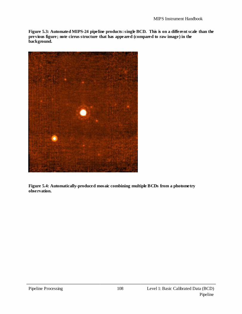
MIPS Instrument Handbook
Pipeline Processing 108
Level 1: Basic Calibrated Data (BCD) Pipeline
Figure 5.3: Automated MIPS-24 pipeline products: single BCD. This is on a different scale than the previous figure; note cirrus structure that has appeared (compared to raw image) in the background.
Figure 5.4: Automatically-produced mosaic combining multiple BCDs from a photometry observation.
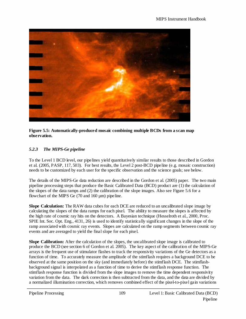
MIPS Instrument Handbook
Pipeline Processing 109
Level 1: Basic Calibrated Data (BCD) Pipeline
Figure 5.5: Automatically-produced mosaic combining multiple BCDs from a scan map observation.
5.2.3 The MIPS-Ge pipeline
To the Level 1 BCD level, our pipelines yield quantitatively similar results to those described in Gordon et al. (2005, PASP, 117, 503). For best results, the Level 2 post-BCD pipeline (e.g. mosaic construction) needs to be customized by each user for the specific observation and the science goals; see below. The details of the MIPS-Ge data reduction are described in the Gordon et al. (2005) paper. The two main pipeline processing steps that produce the Basic Calibrated Data (BCD) product are (1) the calculation of the slopes of the data ramps and (2) the calibration of the slope images. Also see Figure 5.6 for a flowchart of the MIPS Ge (70 and 160 µm) pipeline. Slope Calculation: The RAW data cubes for each DCE are reduced to an uncalibrated slope image by calculating the slopes of the data ramps for each pixel. The ability to measure the slopes is affected by the high rate of cosmic ray hits on the detectors. A Bayesian technique (Hesselroth et al., 2000, Proc. SPIE Int. Soc. Opt. Eng., 4131, 26) is used to identify statistically significant changes in the slope of the ramp associated with cosmic ray events. Slopes are calculated on the ramp segments between cosmic ray events and are averaged to yield the final slope for each pixel. Slope Calibration: After the calculation of the slopes, the uncalibrated slope image is calibrated to produce the BCD (see section 6 of Gordon et al. 2005). The key aspect of the calibration of the MIPS-Ge arrays is the frequent use of stimulator flashes to track the responsivity variations of the Ge detectors as a function of time. To accurately measure the amplitude of the stimflash requires a background DCE to be observed at the same position on the sky (and immediately before) the stimflash DCE. The stimflash-background signal is interpolated as a function of time to derive the stimflash response function. The stimflash response function is divided from the slope images to remove the time dependent responsivity variation from the data. The dark correction is then subtracted from the data, and the data are divided by a normalized illumination correction, which removes combined effect of the pixel-to-pixel gain variations

MIPS Instrument Handbook
Pipeline Processing 110
Level 1: Basic Calibrated Data (BCD) Pipeline
and stimflash illumination pattern. The data are flux-calibrated by applying a flux conversion factor derived from observations of calibrator sources to put the BCDs in units of MJy/sr (surface brightness). The goal of BCD pipeline processing is to produce the best possible data products that can be derived from automated processing. The pipeline produces two BCD products: (1) *_bcd.fits which is the standard calibrated BCD and (2) *_fbcd.fits which is a ''filtered'' bcd product designed for point sources. The fbcd is produced by subtracting off a median of the surrounding DCEs as a function of time per pixel. This filtering technique significantly mitigates the accumulation of stimflash latents and the residual background drifts due to variations of the slow response as a function of time. The application of the median filter removes the background from both the sky and the residual detector effects (i.e., there is a loss of information about the extended background level in the field). Tests show that the application of a median filter maintains point source calibration for scan maps of fields with uniform backgrounds, but the fbcds do not preserve calibration for extended sources or for bright (>~0.2 Jy) point sources within complex emission regions. For extended and/or bright sources, you may achieve better results with offline custom filtering using the GeRT (see section 8.2.3).
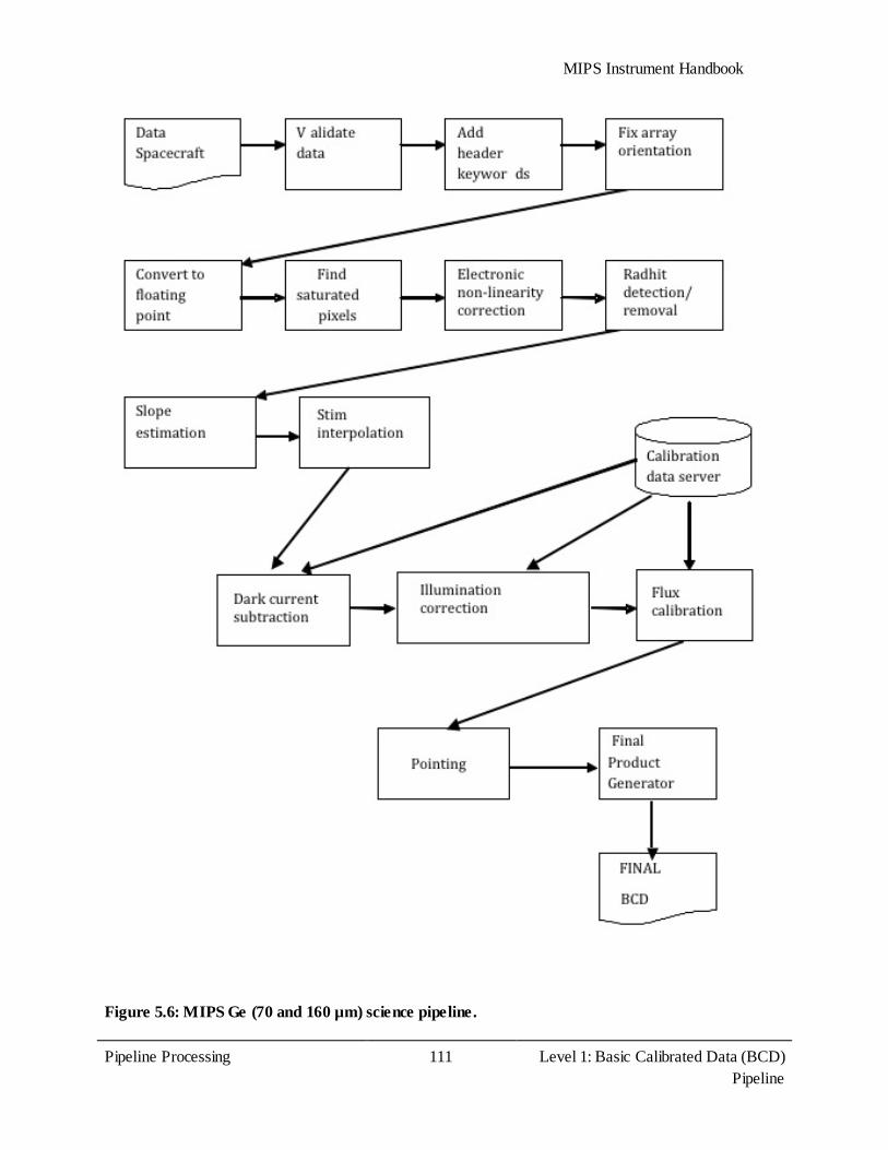
MIPS Instrument Handbook
Pipeline Processing 111
Level 1: Basic Calibrated Data (BCD) Pipeline
Figure 5.6: MIPS Ge (70 and 160 µm) science pipeline.

MIPS Instrument Handbook
Pipeline Processing 112
Level 2: Post-BCD Pipeline
5.2 Level 2: Post-BCD Pipeline
This section, combined with the previous one, covers how your data get reduced, or what we did to your data between when it left the spacecraft and when you get it. The Level 1 BCD products discussed in the previous section are for the most part what you should start with when working with MIPS data. In many cases, you can start with the 24 micron Level 2 post-BCD products. For Ge data in particular, the post-BCD data products are a good way to get an overview of your data, but to do science, you should revert to the Level 1 BCDs and make your own post-BCD products. The Spitzer post-BCD tools can perform tasks including additional corrections for cosmic ray hits, illumination variations, cosmetics, and pointing refinement, as well as basic mosaicking of individual BCDs, source extraction, and bandmerging of point sources. Technically, the suite of post-BCD software is more formally referred to as the ''Advanced Data Products Software,'' because the software is flexible enough to be used with more than just Spitzer data. However, in this context, we will simply refer to it as the ''post-BCD'' software. The post-BCD tools are available in a single package called ''MOPEX.'' In summary, the steps of the post-BCD processing are Background Matching, Pointing Refinement, Basic Mosaicking, Outlier Detection, Astronomical Point Source Extraction (APEX), and finally, Bandmerging of Point Sources. We refer you to the manuals available in the Data Analysis portion of the website for the nitty-gritty of how to run the software; the rest of this chapter addresses MIPS-specific issues and concerns. Suggested namelists for certain situations are given on the website and in the data analysis cookbook. See Figure 5.7 for a simplified flowchart of the post-BCD pipeline.
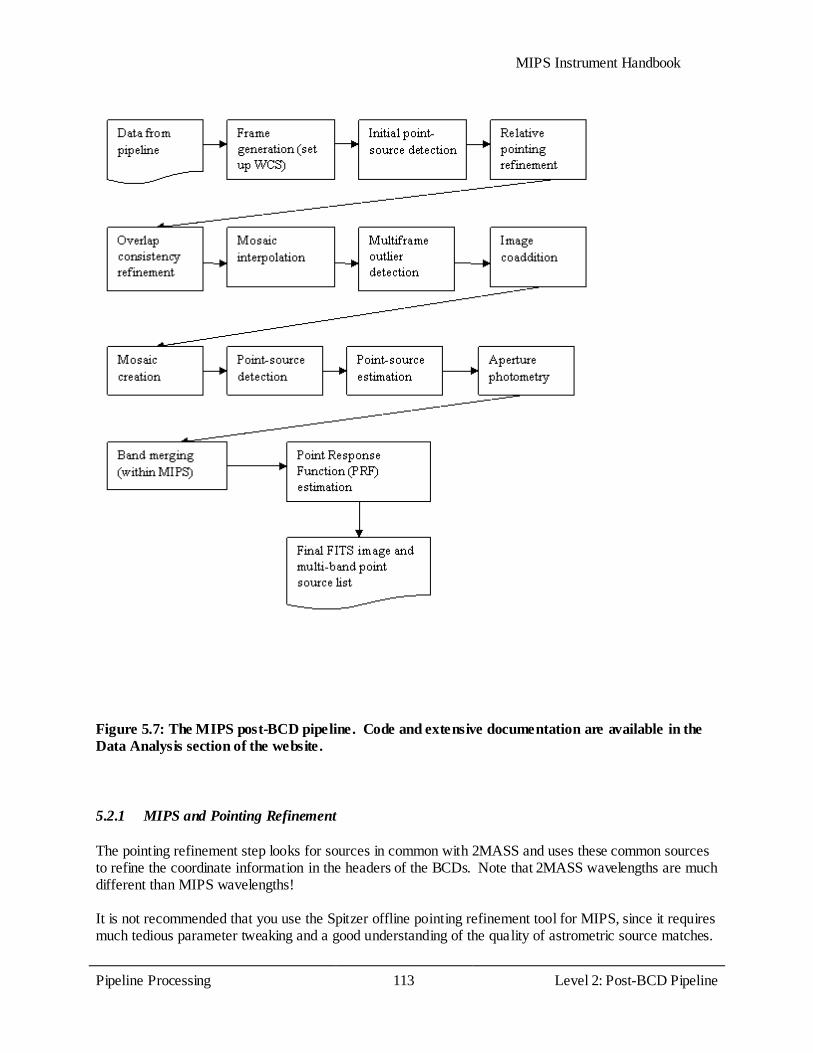
MIPS Instrument Handbook
Pipeline Processing 113
Level 2: Post-BCD Pipeline
Figure 5.7: The MIPS post-BCD pipeline. Code and extensive documentation are available in the Data Analysis section of the website.
5.2.1 MIPS and Pointing Refinement
The pointing refinement step looks for sources in common with 2MASS and uses these common sources to refine the coordinate information in the headers of the BCDs. Note that 2MASS wavelengths are much different than MIPS wavelengths! It is not recommended that you use the Spitzer offline pointing refinement tool for MIPS, since it requires much tedious parameter tweaking and a good understanding of the quality of astrometric source matches.

MIPS Instrument Handbook
Pipeline Processing 114
Level 2: Post-BCD Pipeline
It is important to note that the accuracy of the refined pointing keywords appended to each scan mode BCD FITS header by the SSC strongly depends on the number and quality of the 2MASS-to-24 micron source matches available. Please use these values with care if you by any chance replace the standard BCD WCS with these refined keywords prior to mosaicking. If the mosaic turns out smeared (or sources appear double) then in all likelihood, the refined pointing is suspect and you will need to revert to the raw pointing. In the end, if you do not plan to use these refined pointings, the mosaicker uses the raw image pointing reconstructed from the telescope boresight telemetry and a calibrated model for the scan-mirror. The blind pointing uncertainties of MIPS are currently ~1.2´ ́for 24, ~1.7´ ́for 70, and ~3.9´ ́for 160 microns, all 1 sigma radial. The pointing refinement pipeline will only run on 24 micron scan mode data using exclusively 24 micron point sources that are common with those from the 2MASS public catalog. It operates on the individual scan-legs of scan-mode observation in order to maximize contiguous sky coverage and hence the number of potential 2MASS matches. Earlier testing revealed that 2MASS-to-24 micron point-source matches are very rare in a BCD frame. The online pipeline performs optimum registration of scan-leg mosaics using 2MASS astrometry if a sufficient number of matches exist, then, the refined (intermediate) scan-leg pointings are mapped into the WCS of each BCD frame. Even for large scans, the online pointing refinement pipeline may not yield reliable results (or nothing at all) since 2MASS-to-24 micron matches are far and few between at all galactic latitudes.
5.2.2 MIPS and Mosaicking/Outlier Detection
The mosaicking procedure first includes the projection of BCDs onto a common frame. The projection is done using a linear interpolation (other current options are drizzle and grid, and there are others in development) and takes into account the distortion corrections. The initial projection uses pixel masks for each BCD produced by the pipeline. Remaining pixels affected by cosmic rays that were not detected during the pipeline processing can be flagged using a multiframe spatial-temporal outlier detection (other options include single frame and multiframe spatial). MOPEX keeps track of these outliers in a ''rejection mask'' (*brmsk.fits) and these masks are used when the images are re-projected and mosaicked. (For the specific mosaicking parameters used when running MOPEX as part of the automatic pipeline at the SSC, please see the IRSA website.) The final mosaic is oriented in the file such that the size of the image is minimized; it is generally maximized in the y coordinate, and you can really see this in long scan maps. This means that the mosaics are rotated in order to make the scan direction roughly along the y-axis. Jailbars (see section 7.1.2 below) can be seen in some of the MIPS-24 BCD frames, particularly at the beginning of a scan leg or in frames with saturated sources. By superposition, some of these jailbars are removed in the outlier rejection step of the mosaic construction, but sometimes they persist. The frames can be corrected by applying an additive correction to the affected columns (or portions of columns) at the BCD level, or you may choose to exclude the affected frames entirely from the mosaic construction.
MIPS Instrument Handbook
Data Products 115
Data Products Overview
Chapter 6 Data Products
6.1 Data Products Overview
The nature of the SSC pipeline data processing of MIPS data and the resultant data products are briefly described here and in the following section. In order to fully understand and assess the characteristics of MIPS data, the data processing capabilities, and limitations for the Ge:Ga data in particular, it is important for the observer to carefully examine and understand the photoconductor detector behavior (section 2.3), calibration strategy (sections 4.1.1 and 4.1.2), data acquisition methods (Chapter 3), and how these relate to each other. Gordon et al. (2004, PASP, 117, 503) has more details about the data processing algorithms than are included here. MIPS data are delivered to observers as FITS image files through the archive interface. Because of the complexity and redundant nature of the MIPS AORs, three distinct types of data are generated by the pipeline processing. Observers will be able to select which kinds of data they would like to download through the archive interface. Level 1: Basic Calibrated Data products (BCD) for MIPS are data derived from a single data collection event (a DCE, or a single frame exposure). The Basic Calibrated Data are planned to be the most reliable product achievable by automated processing. BCDs for all AOTs are in the form of FITS images; the SED BCDs are dispersion-corrected and calibrated two-dimensional spectral FITS images. Ge BCD images are corrected for the effects of cosmic ray impacts; cosmic rays are flagged (but not removed) for Si. The total integration time for the individual BCD frames is the observer-specified exposure time (i.e., 3, 4, 10, or 30 seconds), not the total integration time accumulated during the multiple on-source exposures that result from an AOR. No background or sky subtraction is made. BCD products are composed of 2-dimensional FITS image files and a full set of header information keywords, including distortion coefficients, epoch, pointing information, and pipeline and calibration versions. The BCD products are calibrated in MJy/ster. Level 2: Post-BCD products (post-BCD) are derived from a full AOR (e.g., a scan map or a dithered photometry observation). These data are the result of combining all individual BCD frames from a single AOR; in the case of photometry mode, the product is an averaged and registered single image suitable for photometric measurements, and in the case of a scan map, the product is a registered mosaic, with first order removal of seams between the component images. MIPS post-BCD products are calibrated in MJy/ster. The post-BCD products are delivered to the observer in the form of a single FITS image file per AOR, and include a full complement of header keywords. The BCD products are, for the most part, what you should start with when working with MIPS data. For Ge data, in particular, the post-BCD data products are a good way to get an overview of your data; however, to do science, you should revert to the BCDs and make your own post-BCD products. Level 0: Raw Data products are the unprocessed array images (in unprocessed counts per pixel). These FITS image files allow the observer direct access to the data, but still contain the difficult-to-calibrate detector behavior inherent to Ge:Ga detector technology for the 70 µm and 160 µm frames. No cosmic ray removal will have been performed.
MIPS Instrument Handbook
Data Products 116
Data Products Overview
Calibrated Data Units
The Level 1 BCD product, which is the primary data returned to observers after pipeline processing, consists of individual frames where the pixel values are in units of MJy/sr. Jansky is a flux density unit defined as:
1 Jansky = 1 Jy = 10-26 W m-2 Hz-1 = (6.1)
The conversion between Jansky and flux density in W m-2 per unit wavelength is accomplished via
x 10-26 x (6.2)
where the wavelength bin-width is specified in the same length units as and c. For example, if c is taken as 3x1014 µm s-1 and is specified in µm, the above equation results in being in units of W m-2 µm -1.
MIPS Data Processing
Gordon et al. (2005, PASP, 117, 503) has more details about the data processing algorithms than are included here. Basic Calibrated Data (BCD) images are accompanied by additional FITS files. These include, but are not limited to: traceable uncertainties per pixel (an error image), calibration and pipeline reduction pedigree, and data masks for pixels flagged for various data quality criteria. Production of the Level 1 Basic Calibrated Data includes removal of electronic signatures (as applicable) such as a ''droop'' correction in the 24 µm array data (see also chapter Chapter 7), dark current subtraction, non-linearity of sample ramp slopes (Ge:Ga), a robust fitting of ramp slopes to determine total counts per second (Ge:Ga), and the flagging and removal of single or multiple cosmic ray hits using robust Bayesian techniques for the fully sampled Ge:Ga exposure ramps sent to the ground. When possible, corrected ramp segments are adjusted and averaged as required. The inherent redundancy of the MIPS data acquisition adds additional compensation for cosmic ray effects in the combined data. Bad pixels are identified and masked as appropriate. For a uniform diffuse background, the pixels in a BCD image report equal values (within noise statistics; a.k.a. flat fielding of the arrays is performed). The flat field of the Ge:Ga array data is determined and maintained temporally for the Ge:Ga arrays as described in section 4.1.4. Correction of raw counts to flux density per pixel is done based on the detector behavior described elsewhere in this chapter. The flow, or order, of pipeline processing steps appears in Figure 5.1 (the BCD Si pipeline), Figure 5.6 (the BCD Ge pipeline), and Figure 5.7 (the post-BCD pipeline). These pipelines will continue to be refined during operations. The Final BCD products for 24 µm data include (but are not limited to) the following items: slope image, difference image (all zeroes except for pixels saturated in the slope image), replaced image (identical to slope image, except non-zero difference pixels are replaced), error images, and mask images. Note that the 24 µm pipeline does not correct for latent images, and although it flags cosmic rays, it does not correct for them. The Final BCD products for Ge (70 and 160 µm) data similarly include the following items: fully calibrated slope images, the errors associated with the slope images, and mask images. Whether Level 2 post-BCD products are sufficient for a particular program depends upon the specific scientific needs of that program. For example, the MIPS pipeline does not provide the type of refined
MIPS Instrument Handbook
Data Products 117
Data Products Overview
data processing needed to achieve ''super-resolution'' imaging that can be achieved with the available MIPS data acquisition modes. Observers requiring this type of processing in the combining of BCD images will need to apply standard techniques, or develop new ones as required by the demands of the data and/or the science goals. The software used for the Post-BCD pipeline is available (along with copious documentation) in the Data Analysis section of this website. The MIPS post-BCD products are derived per AOR, and do not extend to multiple AORs in an Observer's program. It is composed of FITS image files of size MxN (as defined by the specific observation or map) that are the result of optimally mapping the constituent frames into the post-BCD data frame with minimal loss in resolution. There is one post-BCD FITS file per band per selected wavelength per AOR, except for scan map AORs where there are always 3 files per AOR. The pointing offsets used in mapping of individual frames into the post-BCD products are derived from an optimal offset estimation method, e.g., point source extraction. If insufficient point sources are available, then the data are aligned using spacecraft and CSMM pointing knowledge only. Individual frames are adjusted such that the overlap regions are statistically similar, within the limitations of the large-scale background and slow response characteristics of the Ge:Ga detectors. This implies that some edges might be visible for certain types of varying backgrounds. This will especially be true for adjacent legs of a scan map over a region with significant and varying background. The absolute level to which edge effects and scan leg baseline offsets will be removed in the post-BCD products will not be known with certainty until more flight data are obtained. For observers requiring very uniform maps of extended source regions, there should be some expectation of additional required data processing to correct for edge effects and scan leg baseline offsets in the Ge:Ga data of a scan map. Such effects are minimized in the other MIPS observing modes. The zodiacal backgrounds are maintained only within an individual AOR. Observers who wish to produce maps of areas larger than can be imaged in a single AOR could merge either the individual BCDs or the post-BCD mosaics themselves, in order to obtain the combined dataset. Characterizable Ge:Ga long-term detector behavior are included as part of the processing as needed. No background or sky subtraction is made as part of the post-BCD products processing. Ancillary data images similar to those included with Basic Calibrated Data are also provided with the post-BCD products. The level of MIPS pipeline performance is contingent on proper observation design (one that takes full advantage of the standard MIPS calibration), and a suitable target selection. Suitable target selection includes an assessment of the impact of the general background to be observed during the observation, the MIPS saturation limits, and any bright sources that come within the MIPS fields of view. Absolute pointing knowledge of the focal plane array pixel centers based on the Pointing Control System is better than:
• 24 µm : about 1.4´´, 1 sigma radial • 70 µm : about 1.7´´, 1 sigma radial • 160 µm : about 3.9´´, 1 sigma radial
From the science data frames themselves, refined pointing knowledge of sources must be based on centroiding of objects visible in a MIPS image. The uncertainties will depend on the signal-to-noise ratio of those source detections and the related uncertainty in the centroids, and on the accuracy of prior knowledge of the positions of some or all of the sources. Uncertainty in relative positions between

MIPS Instrument Handbook
Data Products 118
File-Naming Conventions
sources (source offsets) can be much lower than those associated with absolute pointing knowledge, for detections that can support this type of analysis.
6.2 File-Naming Conventions
6.2.1 Level 1: BCDs
All MIPS raw data or BCDs have the same basic filename pattern:
SPITZER_M+chnlnum_aorkey_expid_dcenum_version_type.suffix
The ''M'' stands for MIPS. ''CHNLNUM'' is the header keyword for ''channel number,'' and channel 1 = 24 µm, channel 2 = 70 µm, and channel 3 = 160 µm. The AORKEY (also a header keyword) is a unique 10-digit number assigned to each AOR in our operations database. The EXPID (=exposure id, or number, also a header keyword) and DCENUM (=DCE number, also a header keyword) refers to where in the observing sequence this particular frame was obtained. The ''version'' refers to the number of times that this particular data set has been reprocessed through a validated pipeline. As the understanding of the instrument matured and the pipelines evolved, we reprocessed everything in the Archive, generally multiple times. Finally, ''type'' and ''suffix'' can be any of a variety of abbreviations, referring to the kind of file and its contents, like ''bcd'' and ''fits,'' respectively. The most important MIPS-24 BCD file types for most users will be the *_bcd.fits files for scan mode data and the *_ebcd.fits (enhanced BCD, see section 6.3.4) files for photometry data. For 70 and 160 microns, there are two important BCD files: *_bcd.fits, and *_fbcd.fits. We currently recommend the application of a median high-pass-filter for scan maps of regions containing faint point sources (*_fbcd.fits), and the standard data reduction (*_bcd.fits) for bright and/or extended sources. (See additional discussion below.) A complete list of the types for MIPS-24 are listed in Table 6.1, the types for MIPS-70 and MIPS-160 are listed in Table 6.2. Bit mask definitions for the arrays appear in Table 6.6 for MIPS-24 and Table 6.7 for MIPS-Ge. The bad pixel masks (pmasks) for all the arrays appeared in section 6.5.
6.2.2 Level 2: Post-BCD products
All MIPS post-BCD files have a basic filename pattern that is similar to the BCD files: SPITZER_M+channel_aorkey_dcenum _version_Enum_type.suffix. The letter ''E'' in this example stands for ''ensemble'' product, but it can also be an ''A'' for ''ancillary'' product. In the case of an ensemble product, ''dcenum'' refers to the first dce that was used in the ensemble creation, ''version'' refers to the version of that first dce, and ''Enum'' is the ensemble number. The most important post-BCD file types for most users are the mosaicked files; these provide at the very least a quick look at your data. Most Ge users in particular will want to regenerate the mosaics along with the rest of the post-BCD products with parameters customized for a particular application; see section 8.2 below for some examples.
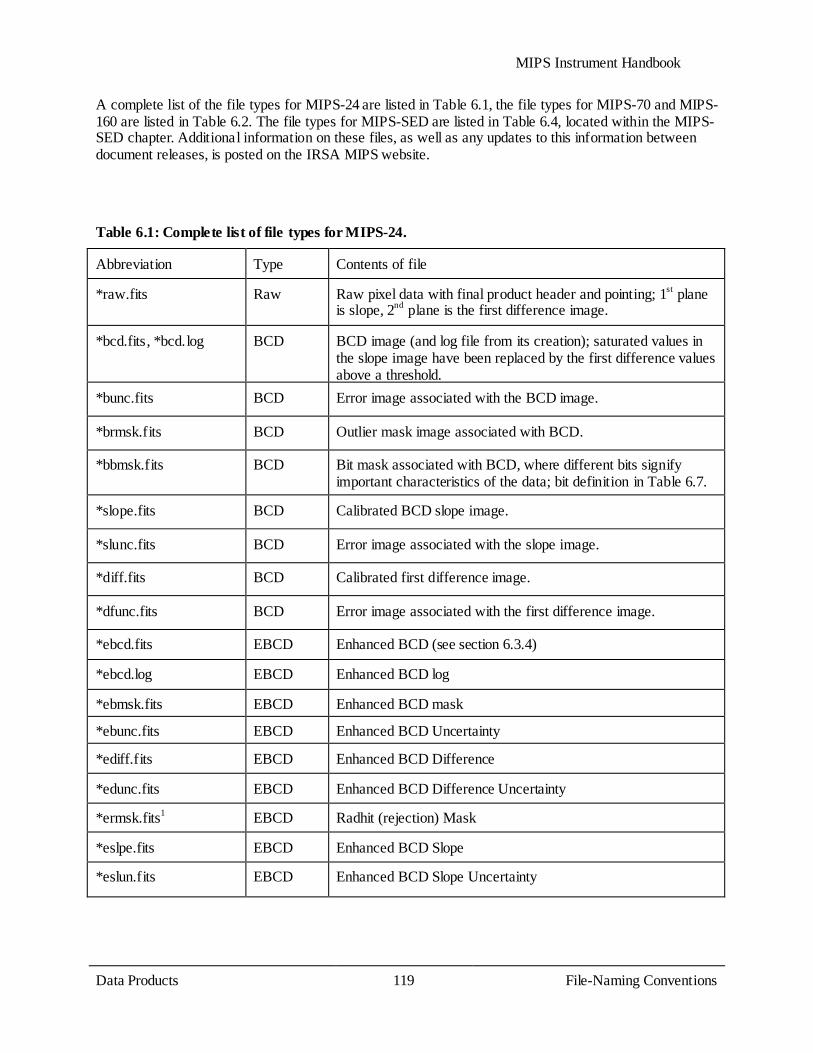
MIPS Instrument Handbook
Data Products 119
File-Naming Conventions
A complete list of the file types for MIPS-24 are listed in Table 6.1, the file types for MIPS-70 and MIPS-160 are listed in Table 6.2. The file types for MIPS-SED are listed in Table 6.4, located within the MIPS-SED chapter. Additional information on these files, as well as any updates to this information between document releases, is posted on the IRSA MIPS website.
Table 6.1: Complete list of file types for MIPS-24.
Abbreviation Type Contents of file
*raw.fits Raw Raw pixel data with final product header and pointing; 1st plane is slope, 2nd plane is the first difference image.
*bcd.fits, *bcd.log BCD BCD image (and log file from its creation); saturated values in the slope image have been replaced by the first difference values above a threshold.
*bunc.fits BCD Error image associated with the BCD image.
*brmsk.fits BCD Outlier mask image associated with BCD.
*bbmsk.fits BCD Bit mask associated with BCD, where different bits signify important characteristics of the data; bit definition in Table 6.7.
*slope.fits BCD Calibrated BCD slope image.
*slunc.fits BCD Error image associated with the slope image.
*diff.fits BCD Calibrated first difference image.
*dfunc.fits BCD Error image associated with the first difference image.
*ebcd.fits EBCD Enhanced BCD (see section 6.3.4)
*ebcd.log EBCD Enhanced BCD log
*ebmsk.fits EBCD Enhanced BCD mask
*ebunc.fits EBCD Enhanced BCD Uncertainty
*ediff.fits EBCD Enhanced BCD Difference
*edunc.fits
EBCD Enhanced BCD Difference Uncertainty
*ermsk.fits1
EBCD Radhit (rejection) Mask
*eslpe.fits EBCD Enhanced BCD Slope
*eslun.fits EBCD Enhanced BCD Slope Uncertainty
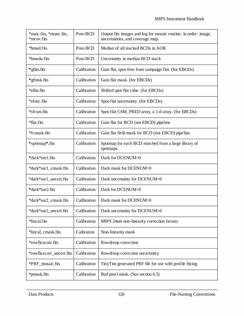
MIPS Instrument Handbook
Data Products 120
File-Naming Conventions
*maic.fits, *munc.fits, *mcov.fits
Post-BCD Output fits images and log for mosaic routine; in order: image, uncertainties, and coverage map.
*bmed.fits Post-BCD Median of all stacked BCDs in AOR
*bmedu.fits Post-BCD Uncertainty in median BCD stack
*gflat.fits Calibration Gain flat, spot-free from campaign flat. (for EBCDs)
*gfmsk.fits Calibration Gain flat mask. (for EBCDs)
*sflat.fits Calibration Shifted spot flat cube. (for EBCDs)
*sfunc.fits
Calibration Spot-flat uncertainty. (for EBCDs)
*sfcsm.fits Calibration Spot-flat CSM_PRED array, a 1-d array. (for EBCDs)
*flat.fits Calibration Gain flat for BCD (not EBCD) pipeline
*fcmask.fits Calibration Gain flat field mask for BCD (not EBCD) pipeline.
*spotmap*.fits Calibration Spotmap for each BCD matched from a large library of spotmaps.
*dark*sur1.fits Calibration Dark for DCENUM=0
*dark*sur1_cmask.fits Calibration Dark mask for DCENUM=0
*dark*sur1_uncert.fits Calibration Dark uncertainty for DCENUM=0
*dark*sur2.fits Calibration Dark for DCENUM>0
*dark*sur2_cmask.fits Calibration Dark mask for DCENUM>0
*dark*sur2_uncert.fits Calibration Dark uncertainty for DCENUM>0
*lincal.fits Calibration MIPS 24um non-linearity correction factors
*lincal_cmask.fits Caibration Non-linearity mask
*rowfluxcorr.fits Calibration Rowdroop correction
*rowfluxcorr_uncert.fits Calibration Rowdroop correction uncertainty
*PRF_mosaic.fits Calibration TinyTim generated PRF file for use with profile fitting
*pmask.fits Calibration Bad pixel mask. (See section 6.5)

MIPS Instrument Handbook
Data Products 121
File-Naming Conventions
*cdelt12_distort.tbl Calibration Cdelt12 distortion coefficents
*fluxconv.tbl Calibration Calibration data file used to convert to MJy/sr
*instrument_fov.tbl Calibration MIPS field of view parameters
*mirrorparameters.tbl Calibration Mirror parameters for pointing transfer
*PRF_Map.tbl Calibration PRF parameters
1Please note that for DCENUM=0, the ersmk.fits (radhit pixel rejection mask) file is not made because it is a product of MOPEX, the mosaicker pipeline, and MOPEX omits data with DCENUM=0 because they are not well-calibrated compared to all the other MIPS-24 data.
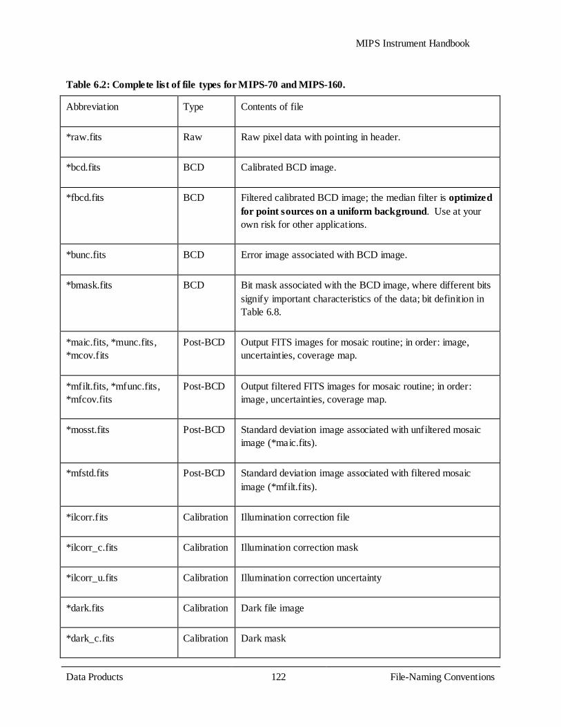
MIPS Instrument Handbook
Data Products 122
File-Naming Conventions
Table 6.2: Complete list of file types for MIPS-70 and MIPS-160.
Abbreviation Type Contents of file
*raw.fits Raw Raw pixel data with pointing in header.
*bcd.fits BCD Calibrated BCD image.
*fbcd.fits BCD Filtered calibrated BCD image; the median filter is optimized for point sources on a uniform background. Use at your own risk for other applications.
*bunc.fits BCD Error image associated with BCD image.
*bmask.fits BCD Bit mask associated with the BCD image, where different bits signify important characteristics of the data; bit definition in Table 6.8.
*maic.fits, *munc.fits, *mcov.fits
Post-BCD Output FITS images for mosaic routine; in order: image, uncertainties, coverage map.
*mfilt.fits, *mfunc.fits, *mfcov.fits
Post-BCD Output filtered FITS images for mosaic routine; in order: image, uncertainties, coverage map.
*mosst.fits Post-BCD Standard deviation image associated with unfiltered mosaic image (*maic.fits).
*mfstd.fits Post-BCD Standard deviation image associated with filtered mosaic image (*mfilt.fits).
*ilcorr.fits Calibration Illumination correction file
*ilcorr_c.fits Calibration Illumination correction mask
*ilcorr_u.fits Calibration Illumination correction uncertainty
*dark.fits Calibration Dark file image
*dark_c.fits Calibration Dark mask

MIPS Instrument Handbook
Data Products 123
Level 1: Basic Calibrated Data (BCD) Products
*dark_u.fits Calibration Dark uncertainty
*enl.fits Calibration Electronic non-linearity
*sat.fits Calibration Hard saturation
*rnoise.fits Calbration Read noise image
*PRF_mosaic.fits Calibration Empirically generated PRF file for use with profile fitting
*pmask.fits Calibration Bad pixel mask. (See section 6.5)
*cdelt12_distort.tbl Calibration Cdelt12 distortion coefficents
*fluxconv.tbl Calibration Calibration data file used to convert to MJy/sr
*instrument_fov.tbl Calibration MIPS field of view parameters
*mirrorparameters.tbl Calibration Mirror parameters for pointing transfer
*PRF_Map.tbl Calibration PRF parameters
6.3 Level 1: Basic Calibrated Data (BCD) Products
6.3.1 Prime vs. Non-Prime Data
Files you think you should have, but don't (or extra files you have but think you shouldn't).
Because all three of the arrays are ''on'' whenever MIPS is on, even if an observation requests just 24 micron data, data are obtained in the other arrays. This makes intuitive sense in the case of scan maps, where valid data are clearly simultaneously obtained in all three arrays. However, what may surprise you is that even for 24 µm photometry mode observations, there are data obtained at both 70 and 160 µm. Note that these other two arrays image slightly different parts of the sky compared to the 24 µm array; they create in the end unfilled maps because the telescope and scan mirror motions are optimized for the 24 µm array. In this specific case, the stimulator frequency is not set properly to obtain useful 70 and 160 µm data. Here, the 24 µm data are the ''prime'' data set, and the Ge data are the ''non-prime'' data. For 70 or 160 micron photometry sequences, the 24 micron data are perfectly fine to use, but they still create an unfilled map. The implications of this data taking strategy are summarized in Table 6.3 below.

MIPS Instrument Handbook
Data Products 124
Level 1: Basic Calibrated Data (BCD) Products
The FITS header keyword PRIMEARR tells you whether data in a given file were obtained with the prime array; PRIMEARR=1 for prime data, 2 for data that are not prime, and 3 for data that are not valid at all (e.g., Ge data during 24 µm photometry). Mosaics are only produced for PRIMEARR=1 Ge data, and BCDs are not even produced for PRIMEARR=3 data. Moreover, in certain scan mirror positions, it is possible to obtain PRIMEARR=3 data for 24 micron data; in this case, the 24 micron array is in the dark. Note also that non-prime 24 micron data may not be correctly flat-fielded given the pick-off mirror contamination; see section 7.1.1. The Archive will serve you non-prime data - it provides BCDs for PRIMEARR=1 or 2, but not 3. It only provides mosaics for PRIMEARR=1, however. If you seem to have much more photometry mode data than you expect, this may be the reason. If you recreate your mosaic and seem to have non-contiguous sky coverage, this may also be the reason - you have combined PRIMEARR=1 and 2 data. If you look at your photometry mosaic and find that the data appear to have missed the target, you are probably looking at your PRIMEARR=2 data rather than your PRIMEARR=1 data; your target will be centered in the PRIMEARR=1 data. Because MIPS BCDs are high quality, most people should not need the raw data, but it is currently provided (for PRIMEARR=1, 2, or 3) through the Archive interface.
Table 6.3: Prime and non-prime data.
Mode ''Prime'' array
Notes on the non-prime data
Scan All three arrays
No non-prime data
24 µm photometry
24 µm Ge data has stims without proper background, covers unfilled portion of sky. PRIMEARR=1 for 24; PRIMEARR=3 for Ge.
70 µm photometry
70 µm 24 and 160 µm data covers unfilled portion of sky, but should produce useful serendipitous data. Mosaics may be produced but may look strange due to the amount of ''dead space.'' PRIMEARR=1 for 70; PRIMEARR=2 for 24 and 160.
160 µm photometry
160 µm 24 and 70 µm data covers unfilled portion of sky, but should produce useful serendipitous data. Mosaics may be produced but may look strange due to the amount of ''dead space.'' PRIMEARR=1 for 160; PRIMEARR=2 for 24 and 70.
6.3.2 MIPS/SED BCDs
BCD images have been fully corrected for all basic instrumental effects. The file names of the SED BCD products follow the same convention as the 70 µm image mode (Table 6.2). However, for the SED mode one should use only the unfiltered BCD images for further analysis or mosaicking.
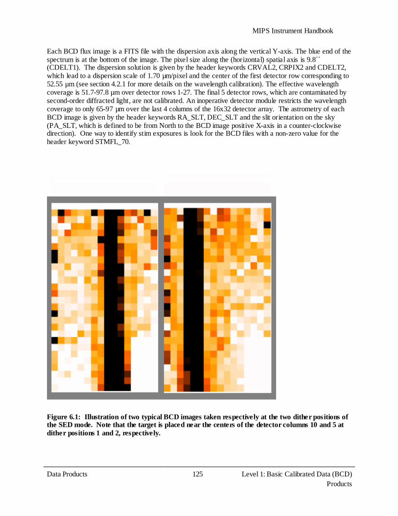
MIPS Instrument Handbook
Data Products 125
Level 1: Basic Calibrated Data (BCD) Products
Each BCD flux image is a FITS file with the dispersion axis along the vertical Y-axis. The blue end of the spectrum is at the bottom of the image. The pixel size along the (horizontal) spatial axis is 9.8´ ́(CDELT1). The dispersion solution is given by the header keywords CRVAL2, CRPIX2 and CDELT2, which lead to a dispersion scale of 1.70 µm/pixel and the center of the first detector row corresponding to 52.55 µm (see section 4.2.1 for more details on the wavelength calibration). The effective wavelength coverage is 51.7-97.8 µm over detector rows 1-27. The final 5 detector rows, which are contaminated by second-order diffracted light, are not calibrated. An inoperative detector module restricts the wavelength coverage to only 65-97 µm over the last 4 columns of the 16x32 detector array. The astrometry of each BCD image is given by the header keywords RA_SLT, DEC_SLT and the slit orientation on the sky (PA_SLT, which is defined to be from North to the BCD image positive X-axis in a counter-clockwise direction). One way to identify stim exposures is look for the BCD files with a non-zero value for the header keyword STMFL_70.
Figure 6.1: Illustration of two typical BCD images taken respectively at the two dither positions of the SED mode. Note that the target is placed near the centers of the detector columns 10 and 5 at dither positions 1 and 2, respectively.

MIPS Instrument Handbook
Data Products 126
Level 1: Basic Calibrated Data (BCD) Products
The SED flux calibration is based on a set of calibration stars with a pre-determined far-infrared spectrum (see section 4.2.3 for more details). The flux scale of a BCD image is in units of MJy sr-1. This is derived from the calibration star observations as follows:
flux scale = Fν(λc)/Σ/A (6.3)
where Fν(λc) is the stellar flux density at the central wavelength λc of the detector pixel under consideration, Σ is the MIPS number counts within an aperture of 5 detector columns centered at the calibration star, and A is the angular size of each detector pixel, which is assumed to be a square of 9.8´́ x 9.8´ .́ As a result, one arrives at a true point-source flux density in Jansky by (i) adding together the BCD pixel values over a 5-detector column aperture centered on the target and then (ii) multiplying the sum by A. For a spectrum of an extended source or a point source extracted with an aperture other than the default one of 5 detector columns, correct fluxes can be derived using the aperture correction factors in Table 4.5 in section 4.2.4. One should also be aware of the fact that the flux scale is calibrated using the sky-subtracted, mosaicked images (see section 4.2.3) of the observed calibration stars. There could be a small systematic flux difference between the two dither positions at the BCD level due to a residual illumination correction issue (see section 4.2.2). It is therefore advised that, if possible, one should always use the mosaicked image for formal photometry. There are a number of remaining issues at the BCD level, including a small spectral tilt of about 1º (given by the BCD header keyword CROTA2) and some small array distortion. Corrections for these issues are addressed in the post-BCD data process (see section 6.4.1).
6.3.3 BCD Uncertainties
The error images currently provided with the 70 and 160 micron BCDs are rough uncertainty estimations and do not include all of the systematic effects associated with the Ge:Ga detectors. These error images also do not include the absolute flux uncertainty. The uncertainties include an empirical error on the slope calculation based on the dispersion of the data along the ramp, an estimated 5% uncertainty on the individual measurements of the stimflash signal, and the errors associated with the DARK and IC (illumination correction) calibration files. The errors on the calibration files represent the dispersion of the calibration DCEs about the median value (per pixel).
6.3.4 Enhanced BCD (EBCD) Products
Beginning in pipeline S18.12, there are two versions of the BCD products for MIPS-24 Photometry data: the original BCDs (bcd.fits) and the enhanced BCDs (ebcd.fits). The BCD and EBCD pipelines differ in the method of flat fielding, as explained below. The EBCDs should, in most cases, have superior flat fielding. The delivered Post-BCD mosaics are made only from the EBCDs (for data from the photometry mode). See Table 6.1 for a complete list of EBCD files. To properly appreciate the difference in the EBCD products, one needs to understand the three different types of flats that are used to flatfield 24 micron data:
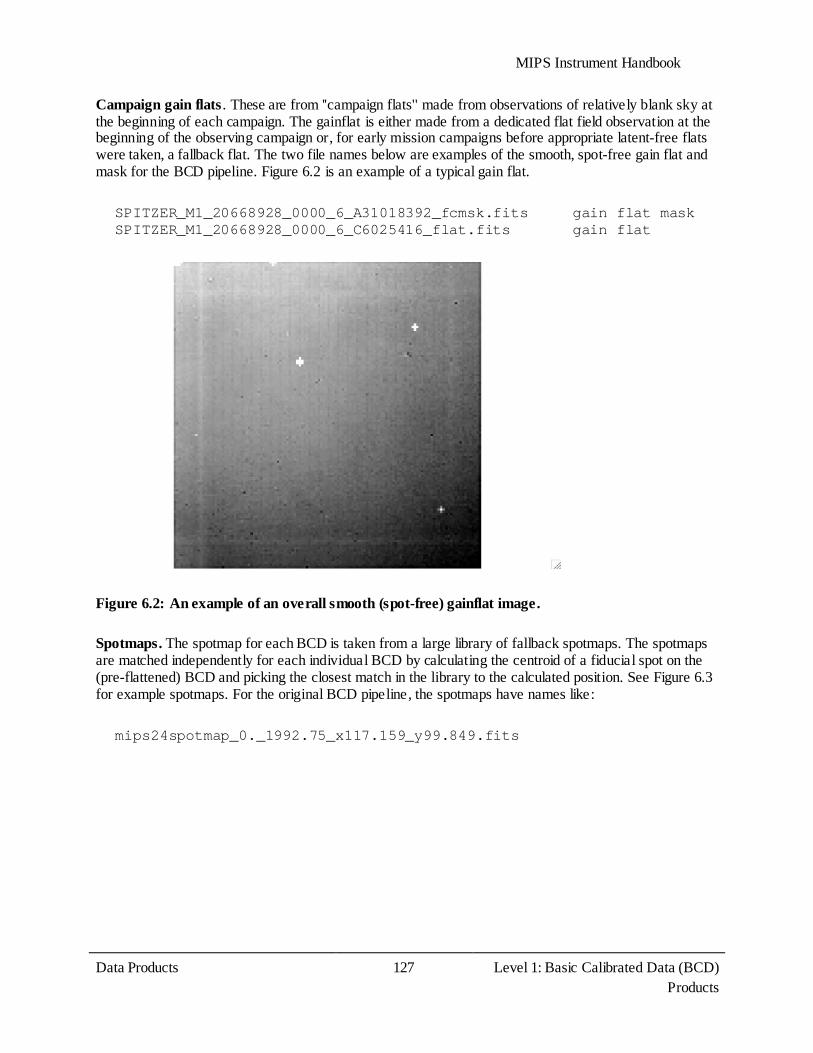
MIPS Instrument Handbook
Data Products 127
Level 1: Basic Calibrated Data (BCD) Products
Campaign gain flats . These are from ''campaign flats'' made from observations of relatively blank sky at the beginning of each campaign. The gainflat is either made from a dedicated flat field observation at the beginning of the observing campaign or, for early mission campaigns before appropriate latent-free flats were taken, a fallback flat. The two file names below are examples of the smooth, spot-free gain flat and mask for the BCD pipeline. Figure 6.2 is an example of a typical gain flat.
SPITZER_M1_20668928_0000_6_A31018392_fcmsk.fits gain flat mask SPITZER_M1_20668928_0000_6_C6025416_flat.fits gain flat
Figure 6.2: An example of an overall smooth (spot-free) gainflat image. Spotmaps. The spotmap for each BCD is taken from a large library of fallback spotmaps. The spotmaps are matched independently for each individual BCD by calculating the centroid of a fiducial spot on the (pre-flattened) BCD and picking the closest match in the library to the calculated position. See Figure 6.3 for example spotmaps. For the original BCD pipeline, the spotmaps have names like:
mips24spotmap_0._1992.75_x117.159_y99.849.fits
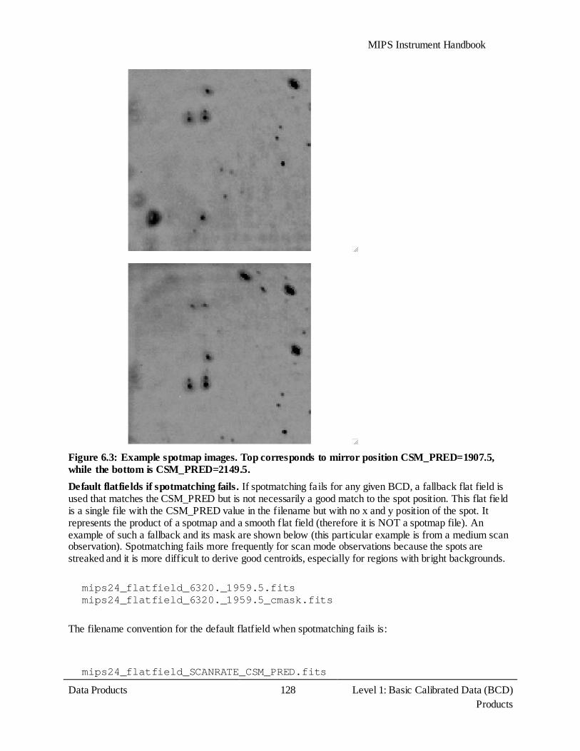
MIPS Instrument Handbook
Data Products 128
Level 1: Basic Calibrated Data (BCD) Products
Figure 6.3: Example spotmap images. Top corresponds to mirror position CSM_PRED=1907.5, while the bottom is CSM_PRED=2149.5. Default flatfields if spotmatching fails. If spotmatching fails for any given BCD, a fallback flat field is used that matches the CSM_PRED but is not necessarily a good match to the spot position. This flat field is a single file with the CSM_PRED value in the filename but with no x and y position of the spot. It represents the product of a spotmap and a smooth flat field (therefore it is NOT a spotmap file). An example of such a fallback and its mask are shown below (this particular example is from a medium scan observation). Spotmatching fails more frequently for scan mode observations because the spots are streaked and it is more difficult to derive good centroids, especially for regions with bright backgrounds.
mips24_flatfield_6320._1959.5.fits mips24_flatfield_6320._1959.5_cmask.fits
The filename convention for the default flatfield when spotmatching fails is:
mips24_flatfield_SCANRATE_CSM_PRED.fits

MIPS Instrument Handbook
Data Products 129
Level 1: Basic Calibrated Data (BCD) Products
Enhanced BCD (EBCD) Flat Fielding
The 24 micron flatfields are the product of a smooth, spot-free gainflat and a ''spotflat'' shifted to match the spot locations in each BCD. For the EBCDs, all of the BCDs in the AOR are used to compute a single spot offset (SPOT_DY) in the y-direction relative to a reference template spotflat file. This single offset shift is applied to all of the planes in the spotflat file. The shifted spotflat file is a cube, matching the spot position of the current AOR, with one plane for each mirror position used in MIPS-24 photometry mode, in ascending order of header keyword CSM_PRED (predicted cryogenic scan mirror position). After shifting the reference to match the current AOR, the appropriate planes are used for flat fielding. In cases of 24 micron data taken in parallel to Ge observations, the improvement in flat fielding could be quite significant. See Figure 6.6 and Figure 6.5 for examples. The headers of these files have explanatory keywords (COMM1,COMM2, etc.) describing the nature of each file.
SPITZER_M1_19241216_0000_6_A31034185_sfunc.fits spot-flat uncert. SPITZER_M1_19241216_0000_6_A31034187_sfcsm.fits spot-flat CSM_PRED array (1-D array) SPITZER_M1_19241216_0000_6_A31034188_gfmsk.fits gain flat mask SPITZER_M1_19241216_0000_6_A31034189_gflat.fits gain flat (spot- free, from campaign flat SPITZER_M1_19241216_0000_6_C6027630_sflat.fits shifted spot flat cube
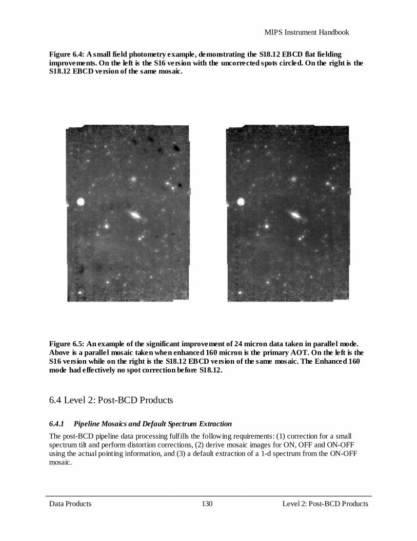
MIPS Instrument Handbook
Data Products 130
Level 2: Post-BCD Products
Figure 6.4: A small field photometry example, demonstrating the S18.12 EBCD flat fielding improvements. On the left is the S16 version with the uncorrected spots circled. On the right is the S18.12 EBCD version of the same mosaic.
Figure 6.5: An example of the significant improvement of 24 micron data taken in parallel mode. Above is a parallel mosaic taken when enhanced 160 micron is the primary AOT. On the left is the S16 version while on the right is the S18.12 EBCD version of the same mosaic. The Enhanced 160 mode had effectively no spot correction before S18.12.
6.4 Level 2: Post-BCD Products
6.4.1 Pipeline Mosaics and Default Spectrum Extraction The post-BCD pipeline data processing fulfills the following requirements: (1) correction for a small spectrum tilt and perform distortion corrections, (2) derive mosaic images for ON, OFF and ON-OFF using the actual pointing information, and (3) a default extraction of a 1-d spectrum from the ON-OFF mosaic.
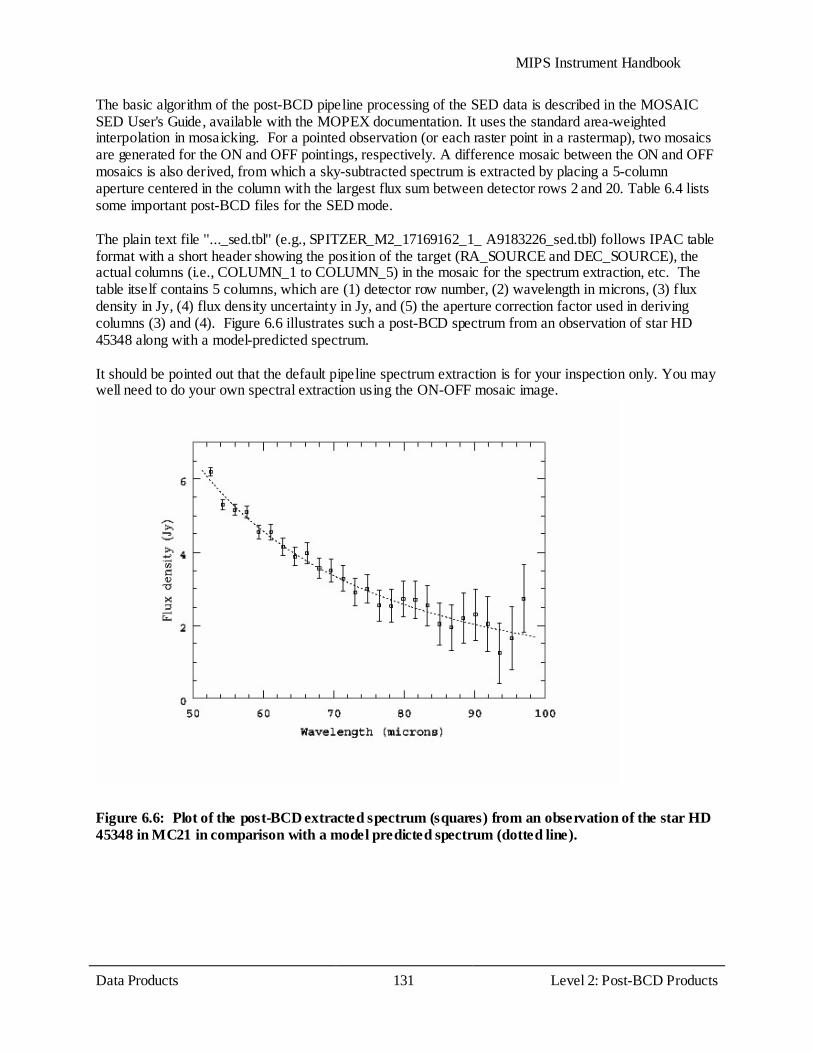
MIPS Instrument Handbook
Data Products 131
Level 2: Post-BCD Products
The basic algorithm of the post-BCD pipeline processing of the SED data is described in the MOSAIC SED User's Guide, available with the MOPEX documentation. It uses the standard area-weighted interpolation in mosaicking. For a pointed observation (or each raster point in a rastermap), two mosaics are generated for the ON and OFF pointings, respectively. A difference mosaic between the ON and OFF mosaics is also derived, from which a sky-subtracted spectrum is extracted by placing a 5-column aperture centered in the column with the largest flux sum between detector rows 2 and 20. Table 6.4 lists some important post-BCD files for the SED mode. The plain text file ''..._sed.tbl'' (e.g., SPITZER_M2_17169162_1_ A9183226_sed.tbl) follows IPAC table format with a short header showing the position of the target (RA_SOURCE and DEC_SOURCE), the actual columns (i.e., COLUMN_1 to COLUMN_5) in the mosaic for the spectrum extraction, etc. The table itself contains 5 columns, which are (1) detector row number, (2) wavelength in microns, (3) flux density in Jy, (4) flux density uncertainty in Jy, and (5) the aperture correction factor used in deriving columns (3) and (4). Figure 6.6 illustrates such a post-BCD spectrum from an observation of star HD 45348 along with a model-predicted spectrum. It should be pointed out that the default pipeline spectrum extraction is for your inspection only. You may well need to do your own spectral extraction using the ON-OFF mosaic image.
Figure 6.6: Plot of the post-BCD extracted spectrum (squares) from an observation of the star HD 45348 in MC21 in comparison with a model predicted spectrum (dotted line).
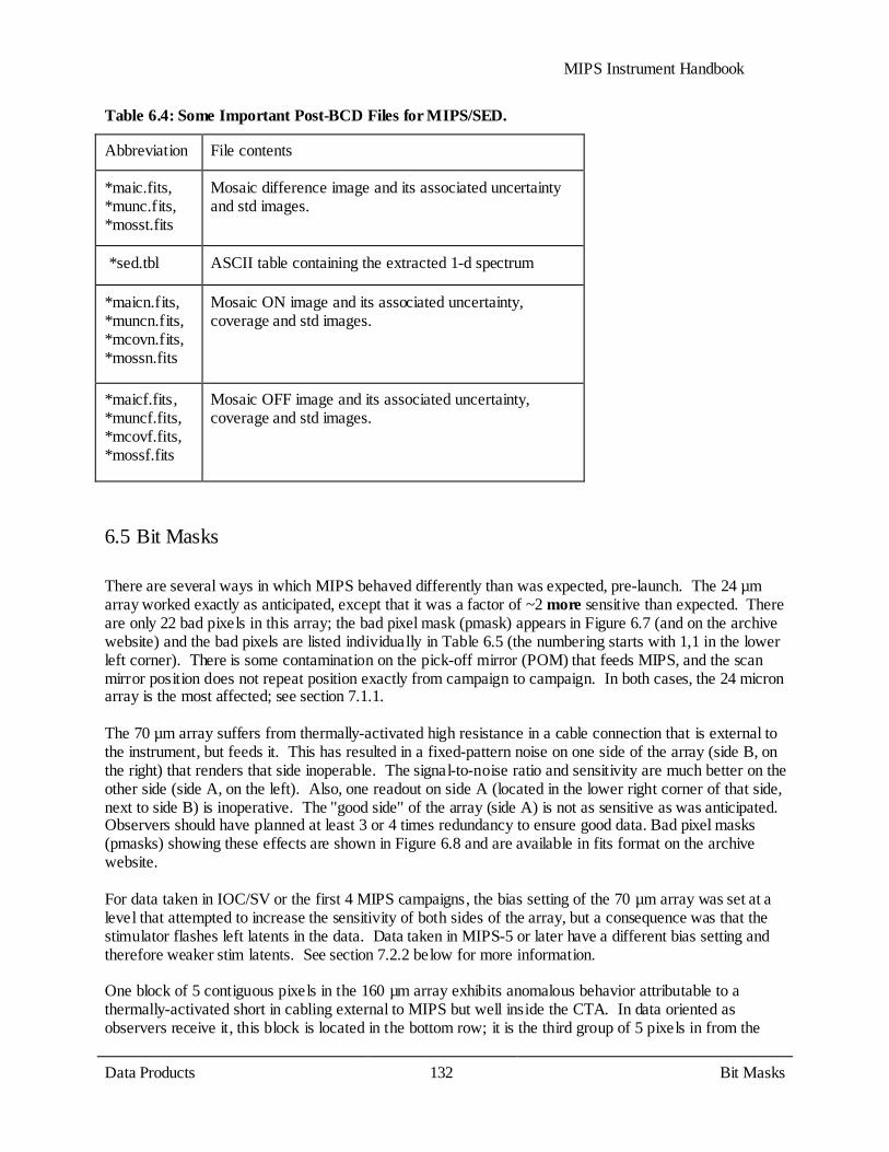
MIPS Instrument Handbook
Data Products 132
Bit Masks
Table 6.4: Some Important Post-BCD Files for MIPS/SED.
Abbreviation File contents
*maic.fits, *munc.fits, *mosst.fits
Mosaic difference image and its associated uncertainty and std images.
*sed.tbl ASCII table containing the extracted 1-d spectrum
*maicn.fits, *muncn.fits, *mcovn.fits, *mossn.fits
Mosaic ON image and its associated uncertainty, coverage and std images.
*maicf.fits, *muncf.fits, *mcovf.fits, *mossf.fits
Mosaic OFF image and its associated uncertainty, coverage and std images.
6.5 Bit Masks
There are several ways in which MIPS behaved differently than was expected, pre-launch. The 24 µm array worked exactly as anticipated, except that it was a factor of ~2 more sensitive than expected. There are only 22 bad pixels in this array; the bad pixel mask (pmask) appears in Figure 6.7 (and on the archive website) and the bad pixels are listed individually in Table 6.5 (the numbering starts with 1,1 in the lower left corner). There is some contamination on the pick-off mirror (POM) that feeds MIPS, and the scan mirror position does not repeat position exactly from campaign to campaign. In both cases, the 24 micron array is the most affected; see section 7.1.1. The 70 µm array suffers from thermally-activated high resistance in a cable connection that is external to the instrument, but feeds it. This has resulted in a fixed-pattern noise on one side of the array (side B, on the right) that renders that side inoperable. The signal-to-noise ratio and sensitivity are much better on the other side (side A, on the left). Also, one readout on side A (located in the lower right corner of that side, next to side B) is inoperative. The ''good side'' of the array (side A) is not as sensitive as was anticipated. Observers should have planned at least 3 or 4 times redundancy to ensure good data. Bad pixel masks (pmasks) showing these effects are shown in Figure 6.8 and are available in fits format on the archive website. For data taken in IOC/SV or the first 4 MIPS campaigns, the bias setting of the 70 µm array was set at a level that attempted to increase the sensitivity of both sides of the array, but a consequence was that the stimulator flashes left latents in the data. Data taken in MIPS-5 or later have a different bias setting and therefore weaker stim latents. See section 7.2.2 below for more information. One block of 5 contiguous pixels in the 160 µm array exhibits anomalous behavior attributable to a thermally-activated short in cabling external to MIPS but well inside the CTA. In data oriented as observers receive it, this block is located in the bottom row; it is the third group of 5 pixels in from the

MIPS Instrument Handbook
Data Products 133
Bit Masks
left. The array is not as sensitive as was anticipated. Observers should have planned at least 3 or 4 times redundancy to ensure good data. Bad pixel masks (pmasks) are shown in Figure 6.9 and are available in FITS format on the archive website. During the early part of the mission, 160 µm signals from K stars were detected to be about a factor of five stronger than expected. Review of the instrument design revealed a weakness in the stray light control that results in a short-wavelength (1-1.6 µm) light leak in this band. See discussion below in section 7.2.6.

MIPS Instrument Handbook
Data Products 134
Bit Masks
Table 6.5: Bad pixels in 24 micron array.
Pixel # (x) Pixel # (y)
1 127
1 128
2 127
2 128
3 127
3 128
4 128
42 128
52 86
52 87
53 85
53 86
53 87
53 88
54 86
54 87
100 101
101 100
101 101
101 102
102 101
112 25

MIPS Instrument Handbook
Data Products 135
Bit Masks
Figure 6.7: Bad pixel mask for 24 microns; black is bad pixels.
Figure 6.8: Bad pixel mask (pmask) for MIPS-70 data. Pink is bad pixels; red is bad half of the array; purple is non-linearity; green is noisier top row and first column. Black is good pixels.

MIPS Instrument Handbook
Data Products 136
Bit Masks
Figure 6.9: Bad pixel mask (pmask) for MIPS-160 data. The center stripe has no detectors (see SOM for details), and the ''bite'' in the lower right is the inoperative readout.
Table 6.6: BCD bit mask definitions for 24 microns found in bbmsk.fits or ebmsk.fits files.
Bit Condition
0 Incomplete or questionable row-droop correction (rowdroop)
1 No row-droop correction applied (rowdroop)
2 Hard saturated (satmask)
3 Read-2 correction could not be applied (rowfluxcorr)
4 Soft saturation corrected and slope value replaced by difference value (desatslope and satmask) (Note: replacement only matters for those pixels that are soft-saturated, e.g., those for which the first difference exceeds a threshold).
5 Latent-image flag. (Note: this bit is set for ebmsk but not bbmsk files in photometry mode. It is set for bbmsk files in scan mode.)
6 Droop removed using questionable value (droopop). (Note: if the pixel is saturated or actually missing from the downlink [bits 13 and 14 respectively], the droop correction will be unreliable.)
7 Flat field applied using questionable valule (flatap)
8 Flat field could not be applied (flatap)
9 Radhit detection (radhitmedfilt)
10
11 Pixel masked in pmask - bad hardware state (satmask)
12 Non-linearity correction could not be computed (slopecorr)
13 Soft saturated (satmask)
14 Data missing in downlink (cvti2r4)
15 reserved: sign bit

MIPS Instrument Handbook
Data Products 137
Header Keywords
Table 6.7: Bit mask definitions for Ge data.
Bit Condition
PMASK
2 Noisy Pixel
3 Bad electronic nonlinearity
8 Bad half of 70 micron array
14 Bad pixel (e.g., bad readout)
15 reserved: sign bit
BMASK
0 Stimflash DCE
3 Saturated sample(s) found in raw data
5 Data near stimflash warning
6 Stim extrapolation warning
8 Raw DCE has missing sample(s)
9 Radhit(s) found in raw data
10 Uncertainty Status
11 Bad pixel as defined by the PMASK
12 Slope calibration failed
13 Slope calculation failed
14 Missing layer, NaN, and/or bad data)
15 Reserved: sign bit
CMASK
13 No valid calibration
15 Reserved: sign bit
6.6 Header Keywords

MIPS Instrument Handbook
Data Products 138
Header Keywords
As with other NASA observatory data, there are many, many header keywords in BCD data, many of which pertain to instrument telemetry rather than astronomy, per se. This section highlights the most important header keywords for BCD MIPS data. A comprehensive list of the BCD header keywords are available in Appendix C. Most of the usual FITS header keywords you expect appear in both the BCD and post-BCD products (CRVAL1 and 2, CRPIX1 and 2, BUNIT, etc.). Here, we highlight some Spitzer-specific keywords of interest. AORLABEL is the name of the AOR as defined by the observer requesting the observations. This name is unique for each AOR within the program, but it is not unique to the entire mission (which is why we have the AORKEY as well, see next paragraph below). OBJECT is the observer-defined target name, and may or may not relate directly to the AORLABEL. (See section 6.2 above for how to determine the AOR label and target for any given AOR.) PROGID is the program identifier for the program that contains the AOR that was used to obtain the data in question; see section 6.2 above for why this can be useful. Each AOR has a 10-digit number called the AORKEY, which is, in fact, unique to each observation for the entire Spitzer project. This value is mostly designed to be only computer-readable, but may be of use for, e.g., corresponding with the SSC regarding a specific AOR. The AORKEY is a header keyword, and is also part of the filename for each BCD. Other elements of the filename (CHNLNUM, EXPID, DCENUM) are also header keywords. AOT_TYPE tells you if the data were taken in scan or photometry mode (or in any of the other MIPS modes). This is particularly useful for double-checking the pixel scale of your 70 µm observations (fine or default). FOVNAME is the name of the field of view used for the observations; see Table 2.1 for a comprehensive list. PRIMEARR tells you if the current data is 'prime' or not; see section 6.3.1 for more on these issues. CREATOR includes the SSC software version, e.g., S13 (see sections 5.1.2 and 5.2.3). DATE_OBS is the time at the start of the AOR, good to within at least 1 second. There are many other times in the header, but if the specific time of the start of your AOR matters, this is the one to use. ANNLTIME is time since the last Ge anneal. FILTERS gives the information about how the *.fbcd files were produced. WARMFLAG indicates whether data were taken during a COLD or WARM 160 micron campaign. STMFL_70 and STMFL_160 tell whether the image (70 µm or 160 µm, depending on keyword) is a calibration stim flash (see section 4.1.1). Any number greater than 0 indicates that it is a stim flash frame. CSM_PRED is the predicted mirror start position. Flattening at 24 µm of each BCD depends on the scan mirror position. The exact postion is a bit uncertain (and that is why the SSC developed a special flattening procedure for 24um), but the best indicator is the "CSM_PRED" header keyword. Indeed the individual flat frames at 24um delivered in the CAL subdirectory are named using this value (or close to this value) as an indicator. The file "mips24spotmap_0._1864.75_x116.501_y126.310.fits" was applied for a CSM_PRED = 1864.75. Under the PHOTOMETRY section of the header are the keywords BUNIT, the units of the image data, FLUXCONV, the flux conversion factor in units of DN/sec to BUNIT, and GAIN, the electron/DN

MIPS Instrument Handbook
Data Products 139
Header Keywords
conversion. In addition there are three keywords that provide an estimate of the infrared background three main components: ZODY_EST for Zodiacal Light , ISM_EST for Interstellar Medium and CIB_EST for Cosmic Background. For example:
BUNIT = 'MJy/sr ' / Units of image data FLUXCONV= 0.0447 / Flux Conv. factor (DN/s to BUNIT) GAIN = 5. / e/DN conversion ZODY_EST= 39.15104 / [MJy/sr] Zodiacal Background Estimate ISM_EST = 0.1186434 / [MJy/sr] Interstellar Medium Estimate CIB_EST = 0. / [MJy/sr] Cosmic IR Background Estimate
These estimates are per BCD and can be useful when mixing multiple epochs observations to produce a final mosaic. Distortion in Spitzer images is represented through header keywords consistent with the latest FITS standard, a CD Matrix using header keywords CD1_1, CD1_2, CD2_1, and CD2_2. The most versions of your favorite image display programs should be able to handle this, but it is possible some older programs may not. The coordinates and pointing as represented in the RA_HMS and DEC_DMS and related keywords are the actual pointing (in sexigesimal), reconstructed on the ground from telescope and scan mirror telemetry. If you prefer decimal degrees, look at CRVAL1 and CRVAL2. There are also header keywords for predicted and/or requested positions, but these values reflect when the observation was scheduled, not necessarily when (or where) it was actually executed. Somewhat confusingly, some of the keywords that appear in the BCD are redefined in the post-BCD stage. In the BCD, PA is the position angle of axis 2, in degrees E of N, so positive values are counter-clockwise. PXSCAL1 and PXSCAL2 are the scale for axes 1 and 2, respectively, in arcsec/px, at position CRPIX1, CRPIX2. In the Post-BCD, however, CROTA2 is the orientation of axis 2, in degrees W of N, so positive values are clockwise. CDELT1 and CDELT2 are the scales for axes 1 and 2, in degrees per pixel. Note that the predicted pointing header keywords may not necessarily be correct. The spacecraft really is pointing in the correct location, but the header keywords are not necessarily correct.

MIPS Instrument Handbook
Data Features and Artifacts 140
MIPS-24 Features and Artifacts
Chapter 7 Data Features and Artifacts
7.1 MIPS-24 Features and Artifacts
In this chapter, we attempt to summarize the most common things you might encounter in your data. We have not attempted to cover all possible cases, so if you discover in your data something ' interesting' and not listed here, please do not hesitate to let us know. Figure 7.1 and Figure 7.2 show examples of some of the effects in MIPS-24 data discussed in this chapter. Note that the Si pipelines are summarized in section 5.1.2.
Figure 7.1: Sample MIPS-24 photometry mosaic product (several combined BCDs) from before the read-2 correction (see section 5.1.2); the pipeline attempts to remove gradients across the field (such as the one seen here), but often gradients across the array at the 1-2% level remain. Also, note the dark spots (from pick-off mirror contamination, primarily in upper right), and the bright latents (above and below the bright source in the center). The specific pattern of the dark spots as portrayed here comes from the movement of the telescope+scan mirror during the photometry dithers and are only visible at this level in images which do not use scan-mirror dependent flat fields.

MIPS Instrument Handbook
Data Features and Artifacts 141
MIPS-24 Features and Artifacts
Figure 7.2: Sample subsection of MIPS-24 scan map. Note dark latents from bright objects.
7.1.1 Pick-off mirror contamination and systematic pointing: practical information
There is some contamination on the pick-off mirror (POM) that feeds MIPS. These dark spots appear to move with celestial objects during scan mirror moves (dithers). The darkest, most well-defined spots are 3-4 pixels across and are ~15-20% dimmer than surrounding pixels; they are located primarily in the upper right of the 24 µm array; see Figure 7.1, Figure 7.3, and Figure 7.4. There are also diffuse features that have a ~1-5% effect. A map of all of the spots seen during normal scan mirror moves based on 24 micron observations is in Figure 7.5. These spots appear to be stable; there is no evidence for ''growing'' or ''jumping'' spots. The standard MIPS pipeline measures the position of the darkest spots in each BCD to select appropriate flats from our database. Unfortunately, when point sources or bright diffuse structure affect the dark spot positions, the match can be bad. Thus, some individual BCDs may show spot residuals. For BCDs where the processing was unable to find spot centroids, flattening will have been done using a ''fallback'' flat without any spot correction. The pipeline also delivers enhanced BCDs (EBCDs) that use all the frames at
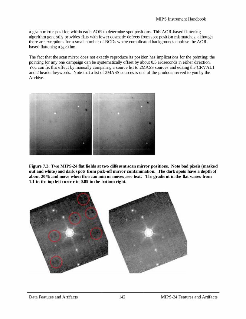
MIPS Instrument Handbook
Data Features and Artifacts 142
MIPS-24 Features and Artifacts
a given mirror position within each AOR to determine spot positions. This AOR-based flattening algorithm generally provides flats with fewer cosmetic defects from spot position mismatches, although there are exceptions for a small number of BCDs where complicated backgrounds confuse the AOR-based flattening algorithm. The fact that the scan mirror does not exactly reproduce its position has implications for the pointing; the pointing for any one campaign can be systematically offset by about 0.5 arcseconds in either direction. You can fix this effect by manually comparing a source list to 2MASS sources and editing the CRVAL1 and 2 header keywords. Note that a list of 2MASS sources is one of the products served to you by the Archive.
Figure 7.3: Two MIPS-24 flat fields at two different scan mirror positions. Note bad pixels (masked out and white) and dark spots from pick-off mirror contamination. The dark spots have a depth of about 20% and move when the scan mirror moves; see text. The gradient in the flat varies from 1.1 in the top left corner to 0.85 in the bottom right.
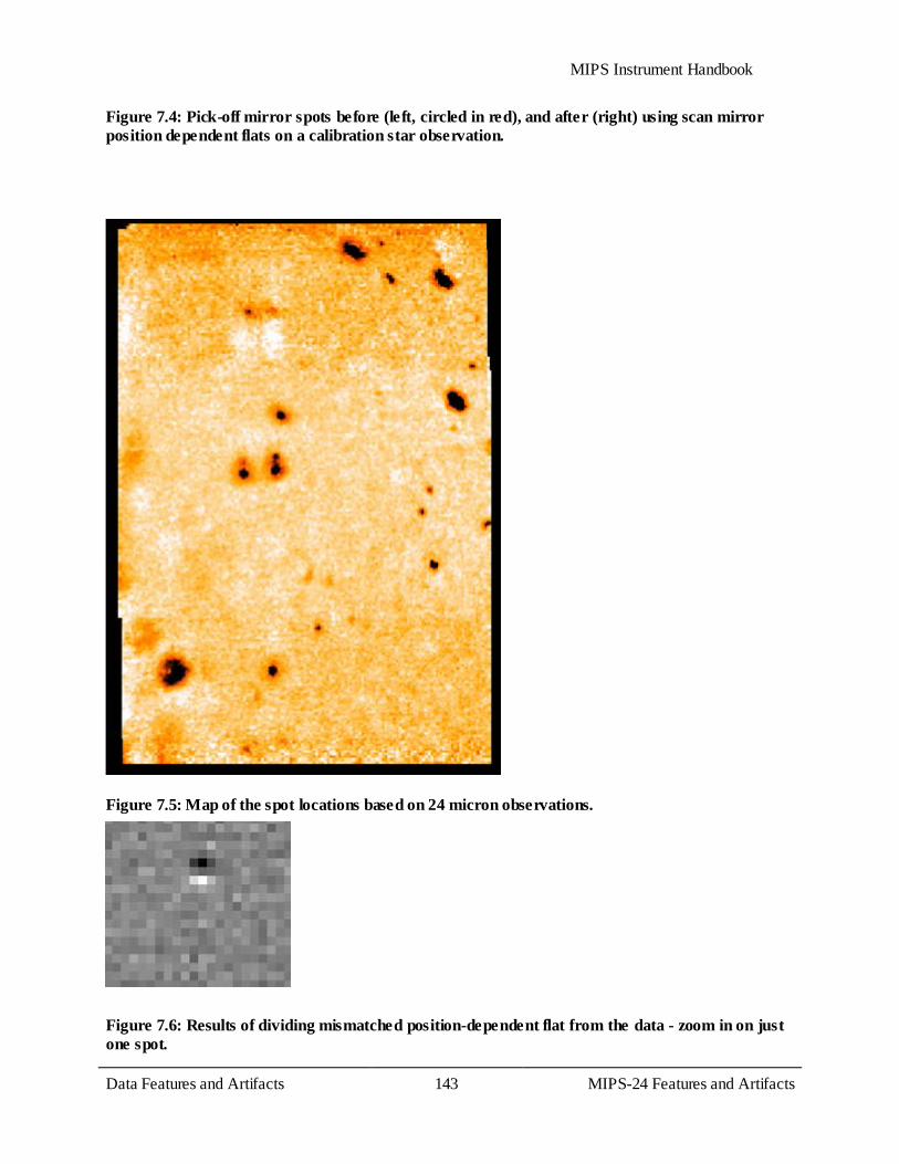
MIPS Instrument Handbook
Data Features and Artifacts 143
MIPS-24 Features and Artifacts
Figure 7.4: Pick-off mirror spots before (left, circled in red), and after (right) using scan mirror position dependent flats on a calibration star observation.
Figure 7.5: Map of the spot locations based on 24 micron observations.
Figure 7.6: Results of dividing mismatched position-dependent flat from the data - zoom in on just one spot.

MIPS Instrument Handbook
Data Features and Artifacts 144
MIPS-24 Features and Artifacts
7.1.2 Jailbars
When a pixel is saturated, a responsivity change occurs in the corresponding readout. This results in a ''jailbar'' pattern occurring every 4th row/column for saturated sources (including some cosmic rays); see Figure 7.7. Only the portion of the array read out after the saturated source is read is affected. Typical effects of jailbars from point sources saturated only in the core produce a decrease in the flux of affected pixels at about the 2 MJy/sr (50 microJy/arcsec2) level, but the magnitude of the effect may vary with source flux. The jailbar effect can occur in a number of different ways. For extended sources, often the saturated regions will cover all 4 or more contiguous readouts and thus an altered responsivity level is seen but no obvious jailbars. One may also see strong jailbars where there are no apparent sources. We believe this effect is due to a highly saturated cosmic ray hit. Faint jailbars are often seen in lower-coverage regions of photometry mosaics where the dither pattern stacks the jailbars. Many of these effects can be mitigated in the post-BCD stage using outlier rejection. The fix for strong jailbars caused by saturated sources is additive - we recommend that you adjust the appropriate column (or portion of the column) additively to match the median level of the unaffected region of the column; see Figure 7.9 and Figure 7.10. There is contributed software for the correction of these strong jailbars available on the Data Analysis section of the website. Weak jailbars are corrected in the BCD pipeline.

MIPS Instrument Handbook
Data Features and Artifacts 145
MIPS-24 Features and Artifacts
Figure 7.7: Example of ''jailbar'' effect from a saturated point source; note that the jailbars are stronger after the bright object. Bright latents (above the source) can also be seen. The central pixel of this bright object is hard saturated (no replacement is available), so it appears black.
7.1.3 Latents
There are three types of MIPS-24 latents: (a) ~0.8% bright latents that last from seconds to 10s of seconds, decay exponentially, look like PSFs, are easily recognizable by eye, and are flagged (but not corrected) by the pipeline; (b) ~2% dark splotchy effects from very bright objects (>50 Jy) that last for hours; and (c) 0.5% bright latents from extremely bright objects that can last for days. (Saturated sources will also produce cosmetically ugly ''jailbars'' (see above), but these are easily recognizable.)
Short-lived bright latents
These are the easiest to recognize by eye or automatically because they always occur in the in-scan direction, and the pipeline does in fact flag them in the mask file (though the pipeline does not remove them). Scan maps leave a trail of latents behind a bright source with spacing which reflects the imaging cadence, Photometry will typically leave latents about 1 arcminute ''above and below'' (i.e. +/- Y) the central source. Examples of this effect can be found in Figure 7.8, as well as Figure 7.1, Figure 7.7, and Figure 7.9. Bright latents are typically not removed by outlier rejection in scan mode because the scan mirror produces repeated overlapping patterns. This is why you may see a trail of latents (often on both sides of a bright source) along the scan direction, particularly for fast scans.
Figure 7.8: Example of short-lived bright latents - note trail of bright dots above the bright source.
Dark latents
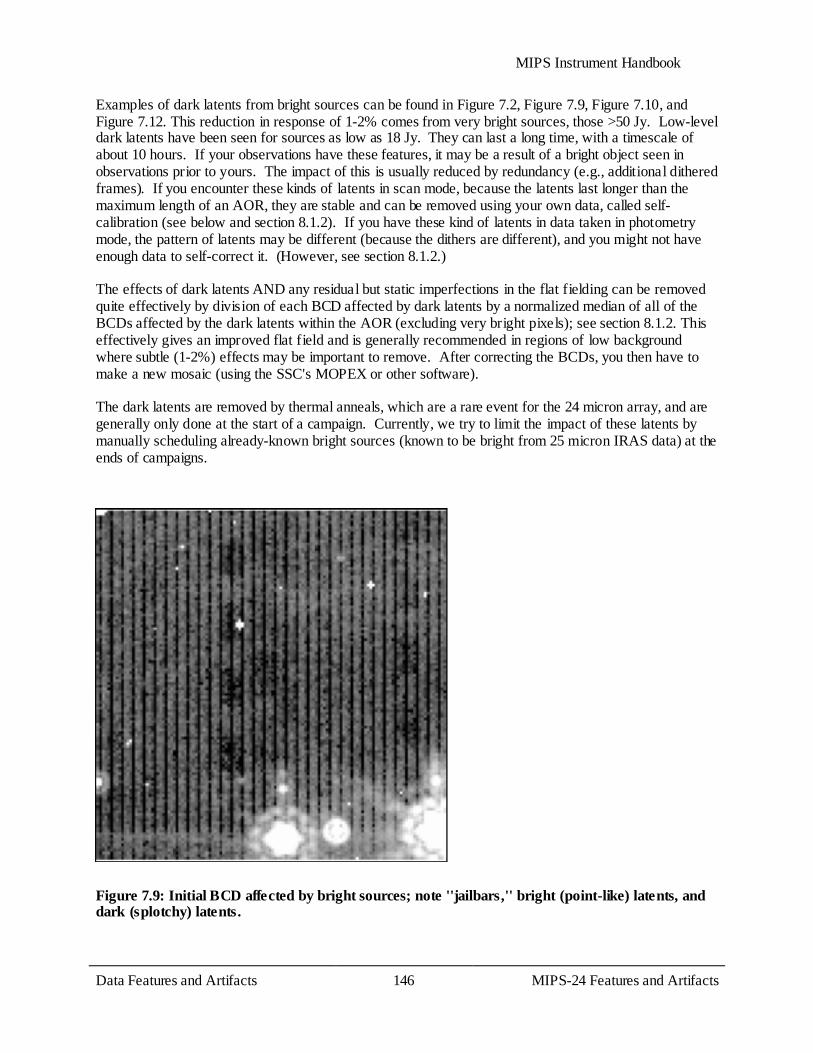
MIPS Instrument Handbook
Data Features and Artifacts 146
MIPS-24 Features and Artifacts
Examples of dark latents from bright sources can be found in Figure 7.2, Figure 7.9, Figure 7.10, and Figure 7.12. This reduction in response of 1-2% comes from very bright sources, those >50 Jy. Low-level dark latents have been seen for sources as low as 18 Jy. They can last a long time, with a timescale of about 10 hours. If your observations have these features, it may be a result of a bright object seen in observations prior to yours. The impact of this is usually reduced by redundancy (e.g., additional dithered frames). If you encounter these kinds of latents in scan mode, because the latents last longer than the maximum length of an AOR, they are stable and can be removed using your own data, called self-calibration (see below and section 8.1.2). If you have these kind of latents in data taken in photometry mode, the pattern of latents may be different (because the dithers are different), and you might not have enough data to self-correct it. (However, see section 8.1.2.) The effects of dark latents AND any residual but static imperfections in the flat fielding can be removed quite effectively by division of each BCD affected by dark latents by a normalized median of all of the BCDs affected by the dark latents within the AOR (excluding very bright pixels); see section 8.1.2. This effectively gives an improved flat field and is generally recommended in regions of low background where subtle (1-2%) effects may be important to remove. After correcting the BCDs, you then have to make a new mosaic (using the SSC's MOPEX or other software). The dark latents are removed by thermal anneals, which are a rare event for the 24 micron array, and are generally only done at the start of a campaign. Currently, we try to limit the impact of these latents by manually scheduling already-known bright sources (known to be bright from 25 micron IRAS data) at the ends of campaigns.
Figure 7.9: Initial BCD affected by bright sources; note ''jailbars,'' bright (point-like) latents, and dark (splotchy) latents.
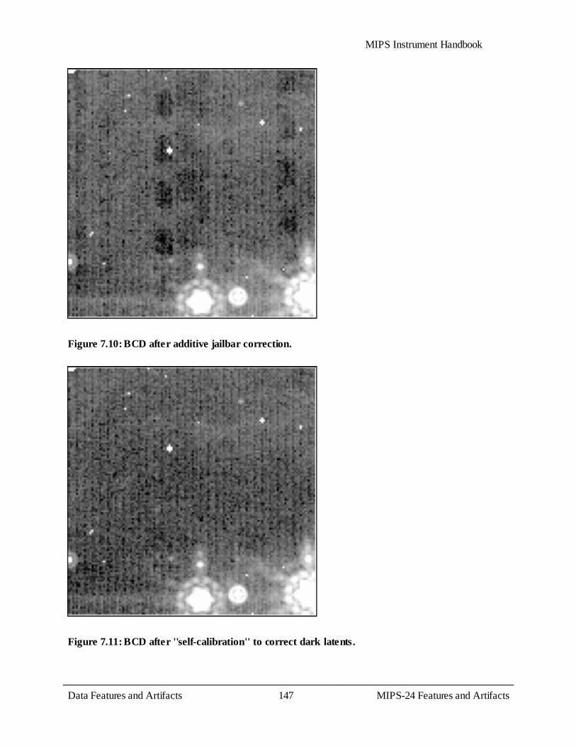
MIPS Instrument Handbook
Data Features and Artifacts 147
MIPS-24 Features and Artifacts
Figure 7.10: BCD after additive jailbar correction.
Figure 7.11: BCD after ''self-calibration'' to correct dark latents.
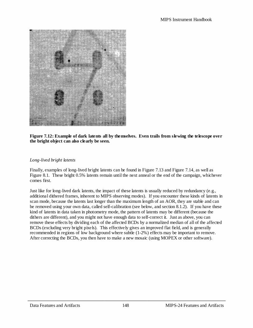
MIPS Instrument Handbook
Data Features and Artifacts 148
MIPS-24 Features and Artifacts
Figure 7.12: Example of dark latents all by themselves. Even trails from slewing the telescope over the bright object can also clearly be seen.
Long-lived bright latents
Finally, examples of long-lived bright latents can be found in Figure 7.13 and Figure 7.14, as well as Figure 8.1. These bright 0.5% latents remain until the next anneal or the end of the campaign, whichever comes first. Just like for long-lived dark latents, the impact of these latents is usually reduced by redundancy (e.g., additional dithered frames, inherent to MIPS observing modes). If you encounter these kinds of latents in scan mode, because the latents last longer than the maximum length of an AOR, they are stable and can be removed using your own data, called self-calibration (see below, and section 8.1.2). If you have these kind of latents in data taken in photometry mode, the pattern of latents may be different (because the dithers are different), and you might not have enough data to self-correct it. Just as above, you can remove these effects by dividing each of the affected BCDs by a normalized median of all of the affected BCDs (excluding very bright pixels). This effectively gives an improved flat field, and is generally recommended in regions of low background where subtle (1-2%) effects may be important to remove. After correcting the BCDs, you then have to make a new mosaic (using MOPEX or other software).
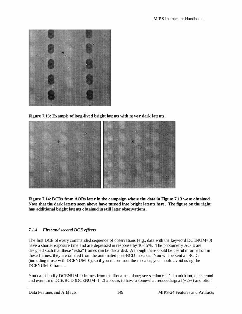
MIPS Instrument Handbook
Data Features and Artifacts 149
MIPS-24 Features and Artifacts
Figure 7.13: Example of long-lived bright latents with newer dark latents.
Figure 7.14: BCDs from AORs later in the campaign where the data in Figure 7.13 were obtained. Note that the dark latents seen above have turned into bright latents here. The figure on the right has additional bright latents obtained in still later observations.
7.1.4 First and second DCE effects
The first DCE of every commanded sequence of observations (e.g., data with the keyword DCENUM=0) have a shorter exposure time and are depressed in response by 10-15%. The photometry AOTs are designed such that these ''extra'' frames can be discarded. Although there could be useful information in these frames, they are omitted from the automated post-BCD mosaics. You will be sent all BCDs (including those with DCENUM=0), so if you reconstruct the mosaics, you should avoid using the DCENUM=0 frames. You can identify DCENUM=0 frames from the filenames alone; see section 6.2.1. In addition, the second and even third DCE/BCD (DCENUM=1, 2) appears to have a somewhat reduced signal (~2%) and often
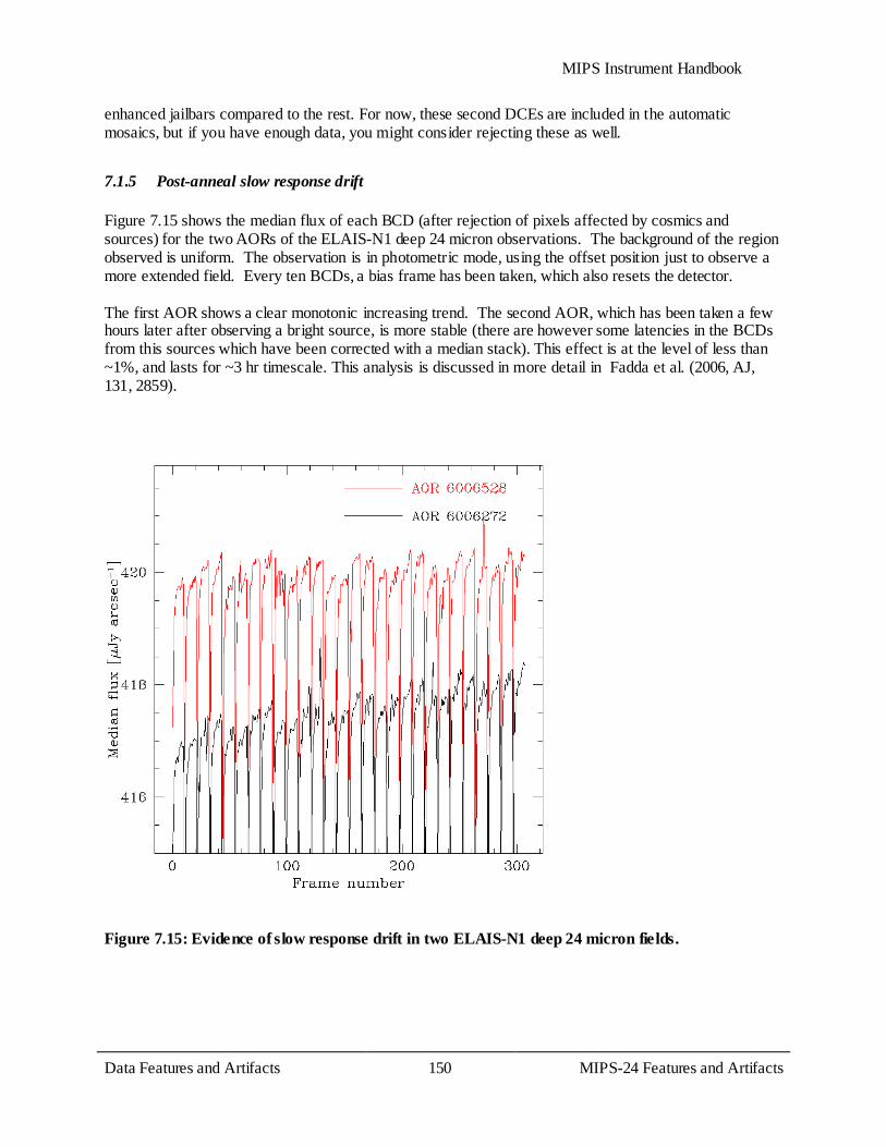
MIPS Instrument Handbook
Data Features and Artifacts 150
MIPS-24 Features and Artifacts
enhanced jailbars compared to the rest. For now, these second DCEs are included in the automatic mosaics, but if you have enough data, you might consider rejecting these as well.
7.1.5 Post-anneal slow response drift
Figure 7.15 shows the median flux of each BCD (after rejection of pixels affected by cosmics and sources) for the two AORs of the ELAIS-N1 deep 24 micron observations. The background of the region observed is uniform. The observation is in photometric mode, using the offset position just to observe a more extended field. Every ten BCDs, a bias frame has been taken, which also resets the detector. The first AOR shows a clear monotonic increasing trend. The second AOR, which has been taken a few hours later after observing a bright source, is more stable (there are however some latencies in the BCDs from this sources which have been corrected with a median stack). This effect is at the level of less than ~1%, and lasts for ~3 hr timescale. This analysis is discussed in more detail in Fadda et al. (2006, AJ, 131, 2859).
Figure 7.15: Evidence of slow response drift in two ELAIS-N1 deep 24 micron fields.
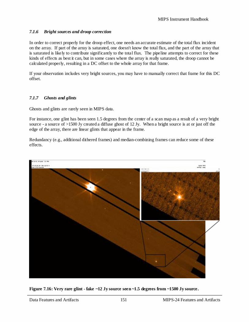
MIPS Instrument Handbook
Data Features and Artifacts 151
MIPS-24 Features and Artifacts
7.1.6 Bright sources and droop correction
In order to correct properly for the droop effect, one needs an accurate estimate of the total flux incident on the array. If part of the array is saturated, one doesn't know the total flux, and the part of the array that is saturated is likely to contribute significantly to the total flux. The pipeline attempts to correct for these kinds of effects as best it can, but in some cases where the array is really saturated, the droop cannot be calculated properly, resulting in a DC offset to the whole array for that frame. If your observation includes very bright sources, you may have to manually correct that frame for this DC offset.
7.1.7 Ghosts and glints
Ghosts and glints are rarely seen in MIPS data. For instance, one glint has been seen 1.5 degrees from the center of a scan map as a result of a very bright source - a source of >1500 Jy created a diffuse ghost of 12 Jy. When a bright source is at or just off the edge of the array, there are linear glints that appear in the frame. Redundancy (e.g., additional dithered frames) and median-combining frames can reduce some of these effects.
Figure 7.16: Very rare glint - fake ~12 Jy source seen ~1.5 degrees from ~1500 Jy source.
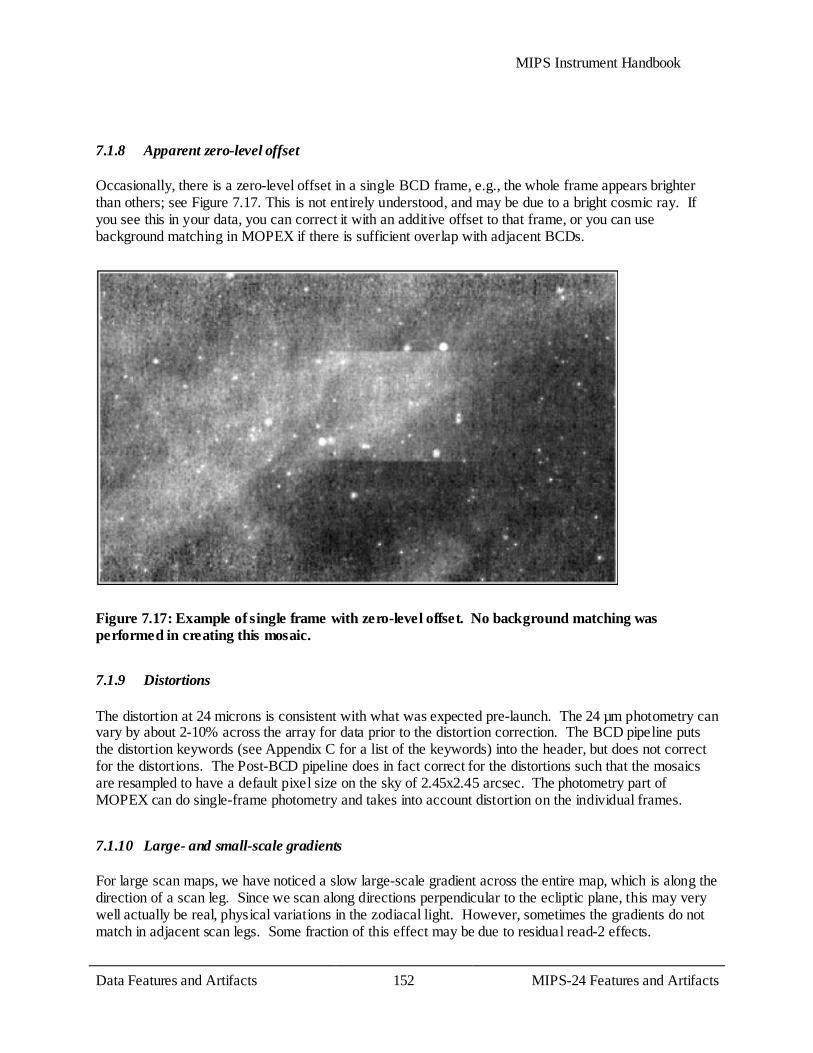
MIPS Instrument Handbook
Data Features and Artifacts 152
MIPS-24 Features and Artifacts
7.1.8 Apparent zero-level offset
Occasionally, there is a zero-level offset in a single BCD frame, e.g., the whole frame appears brighter than others; see Figure 7.17. This is not entirely understood, and may be due to a bright cosmic ray. If you see this in your data, you can correct it with an additive offset to that frame, or you can use background matching in MOPEX if there is sufficient overlap with adjacent BCDs.
Figure 7.17: Example of single frame with zero-level offset. No background matching was performed in creating this mosaic.
7.1.9 Distortions
The distortion at 24 microns is consistent with what was expected pre-launch. The 24 µm photometry can vary by about 2-10% across the array for data prior to the distortion correction. The BCD pipeline puts the distortion keywords (see Appendix C for a list of the keywords) into the header, but does not correct for the distortions. The Post-BCD pipeline does in fact correct for the distortions such that the mosaics are resampled to have a default pixel size on the sky of 2.45x2.45 arcsec. The photometry part of MOPEX can do single-frame photometry and takes into account distortion on the individual frames.
7.1.10 Large- and small-scale gradients
For large scan maps, we have noticed a slow large-scale gradient across the entire map, which is along the direction of a scan leg. Since we scan along directions perpendicular to the ecliptic plane, this may very well actually be real, physical variations in the zodiacal light. However, sometimes the gradients do not match in adjacent scan legs. Some fraction of this effect may be due to residual read-2 effects.
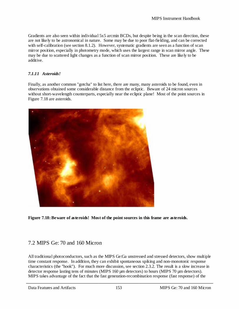
MIPS Instrument Handbook
Data Features and Artifacts 153
MIPS Ge: 70 and 160 Micron
Gradients are also seen within individual 5x5 arcmin BCDs, but despite being in the scan direction, these are not likely to be astronomical in nature. Some may be due to poor flat-fielding, and can be corrected with self-calibration (see section 8.1.2). However, systematic gradients are seen as a function of scan mirror position, especially in photometry mode, which uses the largest range in scan mirror angle. These may be due to scattered light changes as a function of scan mirror position. These are likely to be additive.
7.1.11 Asteroids!
Finally, as another common ''gotcha'' to list here, there are many, many asteroids to be found, even in observations obtained some considerable distance from the ecliptic. Beware of 24 micron sources without short-wavelength counterparts, especially near the ecliptic plane! Most of the point sources in Figure 7.18 are asteroids.
Figure 7.18: Beware of asteroids! Most of the point sources in this frame are asteroids.
7.2 MIPS Ge: 70 and 160 Micron
All traditional photoconductors, such as the MIPS Ge:Ga unstressed and stressed detectors, show multiple time constant response. In addition, they can exhibit spontaneous spiking and non-monotonic response characteristics (the ''hook''). For much more discussion, see section 2.3.2. The result is a slow increase in detector response lasting tens of minutes (MIPS 160 µm detectors) to hours (MIPS 70 µm detectors). MIPS takes advantage of the fact that the fast generation-recombination response (fast response) of the
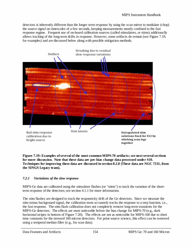
MIPS Instrument Handbook
Data Features and Artifacts 154
MIPS Ge: 70 and 160 Micron
detectors is inherently different than the longer term response by using the scan mirror to modulate (chop) the source signal on timescales of a few seconds, keeping measurements mostly confined to the fast response regime. Frequent use of on-board calibration sources (called stimulators, or stims) additionally allows tracking of the long-term drifts in response. However, some artifacts do remain (see Figure 7.19, for examples) and are discussed below along with possible mitigation methods.
Figure 7.19: Examples of several of the most common MIPS-70 artifacts; see next several sections for more discussion. Note that these data are pre-bias change data processed under S10. Techniques for improving these data are discussed in section 8.2.8 (These data are NGC 7331, from the SINGS Legacy team).
7.2.1 Variations of the slow response
MIPS-Ge data are calibrated using the stimulator flashes (or ''stims'') to track the variation of the short-term response of the detectors; see section 4.1.1 for more information. The stim flashes are designed to track the responsivity drift of the Ge detectors. Since we measure the stim minus background signal, the calibration most accurately tracks the response to a step function, i.e., the fast response. The stim flash calibration does not completely remove long-term transients for the MIPS-Ge detectors. The effects are most noticeable before the bias change for MIPS-70 (e.g., dark horizontal stripes in bottom of Figure 7.20). The effects are not as noticeable for MIPS-160 due to short time constants for the stressed 160 micron detectors. For point source science, this effect can be removed using a temporal median filter (e.g., for scan data).
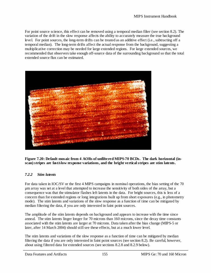
MIPS Instrument Handbook
Data Features and Artifacts 155
MIPS Ge: 70 and 160 Micron
For point source science, this effect can be removed using a temporal median filter (see section 8.2). The variation of the drift in the slow response affects the ability to accurately measure the true background level. For point sources, the long-term drifts can be treated as an additive effect (i.e., subtracting off a temporal median). The long-term drifts affect the actual response from the background, suggesting a multiplicative correction may be needed for large extended regions. For large extended sources, we recommended that observers take enough off-source data of the surrounding background so that the total extended source flux can be estimated.
Figure 7.20: Default mosaic from 4 AORs of unfiltered MIPS-70 BCDs. The dark horizontal (in-scan) stripes are fast/slow response variations, and the bright vertical stripes are stim latents.
7.2.2 Stim latents
For data taken in IOC/SV or the first 4 MIPS campaigns in nominal operations, the bias setting of the 70 µm array was set at a level that attempted to increase the sensitivity of both sides of the array, but a consequence was that the stimulator flashes left latents in the data. For bright sources, this is less of a concern than for extended regions or long integrations built up from short exposures (e.g., in photometry mode). The stim latents and variations of the slow response as a function of time can be mitigated by median filtering the data, if you are only interested in faint point sources. The amplitude of the stim latents depends on background and appears to increase with the time since anneal. The stim latents linger longer for 70 microns than 160 microns, since the decay time constants associated with the stim latents are larger at 70 microns. Data taken after the bias change (MIPS-5 or later, after 14 March 2004) should still see these effects, but at a much lower level. The stim latents and variations of the slow response as a function of time can be mitigated by median filtering the data if you are only interested in faint point sources (see section 8.2). Be careful, however, about using filtered data for extended sources (see sections 8.2.8 and 8.2.9 below).
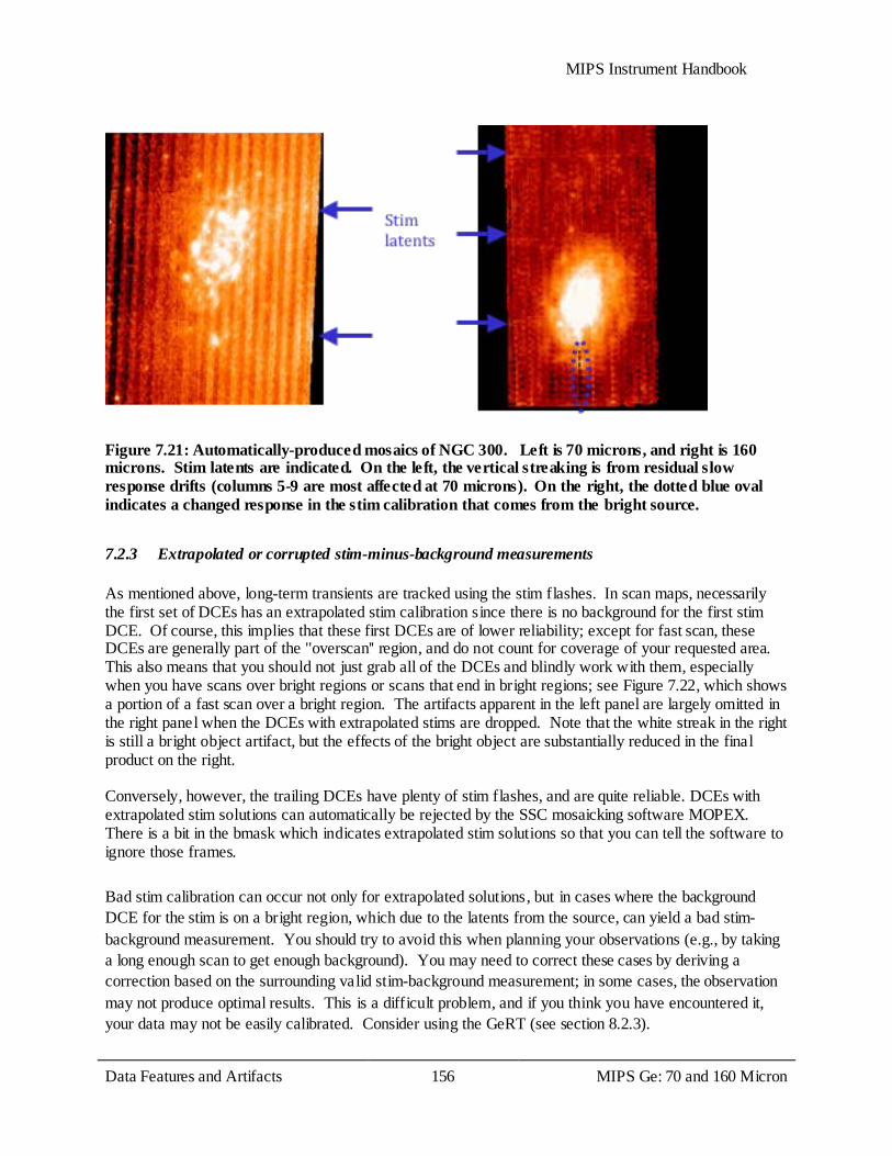
MIPS Instrument Handbook
Data Features and Artifacts 156
MIPS Ge: 70 and 160 Micron
Figure 7.21: Automatically-produced mosaics of NGC 300. Left is 70 microns, and right is 160 microns. Stim latents are indicated. On the left, the vertical streaking is from residual slow response drifts (columns 5-9 are most affected at 70 microns). On the right, the dotted blue oval indicates a changed response in the stim calibration that comes from the bright source.
7.2.3 Extrapolated or corrupted stim-minus-background measurements
As mentioned above, long-term transients are tracked using the stim flashes. In scan maps, necessarily the first set of DCEs has an extrapolated stim calibration since there is no background for the first stim DCE. Of course, this implies that these first DCEs are of lower reliability; except for fast scan, these DCEs are generally part of the ''overscan'' region, and do not count for coverage of your requested area. This also means that you should not just grab all of the DCEs and blindly work with them, especially when you have scans over bright regions or scans that end in bright regions; see Figure 7.22, which shows a portion of a fast scan over a bright region. The artifacts apparent in the left panel are largely omitted in the right panel when the DCEs with extrapolated stims are dropped. Note that the white streak in the right is still a bright object artifact, but the effects of the bright object are substantially reduced in the final product on the right. Conversely, however, the trailing DCEs have plenty of stim flashes, and are quite reliable. DCEs with extrapolated stim solutions can automatically be rejected by the SSC mosaicking software MOPEX. There is a bit in the bmask which indicates extrapolated stim solutions so that you can tell the software to ignore those frames.
Bad stim calibration can occur not only for extrapolated solutions, but in cases where the background DCE for the stim is on a bright region, which due to the latents from the source, can yield a bad stim-background measurement. You should try to avoid this when planning your observations (e.g., by taking a long enough scan to get enough background). You may need to correct these cases by deriving a correction based on the surrounding valid stim-background measurement; in some cases, the observation may not produce optimal results. This is a difficult problem, and if you think you have encountered it, your data may not be easily calibrated. Consider using the GeRT (see section 8.2.3).
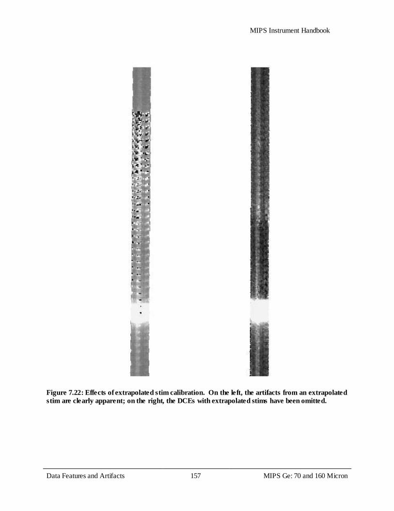
MIPS Instrument Handbook
Data Features and Artifacts 157
MIPS Ge: 70 and 160 Micron
Figure 7.22: Effects of extrapolated stim calibration. On the left, the artifacts from an extrapolated stim are clearly apparent; on the right, the DCEs with extrapolated stims have been omitted.
MIPS Instrument Handbook
Data Features and Artifacts 158
MIPS Ge: 70 and 160 Micron
7.2.4 Electronic non-linearities
The electronic non-linearities for the MIPS-Ge detectors are corrected for in the online pipeline. However, spurious electronic non-linearity solutions for a few unstable pixels on the top row of the 70 micron detector can yield artifacts in the mosaics. The recommended solution is to make sure you have the most recent pmask, and make mosaics with this updated pmask, ignoring these pixels (use the pmask rejection parameter=16648).
7.2.5 Flux non-linearities
The flux nonlinearities for the MIPS-Ge detectors represent the differences in the flux conversion factor as a function of source flux. Thre pipeline assumes a constant flux conversion factor for all flux ranges. MIPS 70 micron sources show significant (~40%) flux non-linearities over the range from 22 mJy to 17 Jy, although the use of PSF-fitted photometry rather than aperture photometry greatly reduces this effect (see Gordon et al. 2007, PASP, 119, 1019). The overall behavior of the 160 micron stressed Ge:Ga array is linear between 0.1 and 2 Jy (Stansberry et al 2007, PASP, 119, 1038). Continuing up to 4 Jy, 160 micron shows a departure of ~10% from linearity for point sources.
7.2.6 160 µm short-wavelength light leak
Signals on pure photospheres of stars at 160 µm are stronger than expected by about a factor of five. Review of the instrument design has revealed a weakness in the stray light control that could result in a short wavelength Ge:Ga response being detected in this band (due to scattering off a blocking filter). For many types of observations, this light leak does not impact the data at all. Stars fainter than mJ ~ 5.5 mag will not be detectable in the leak above the confusion level. No compact extragalactic sources have mJ brighter than 5.5 mag. The leak signal for a star of mJ = -0.5 mag is equivalent to ~ 2.5 Jy at 160 µm. The parameter to consider for any given target is the 160 µm /2 µm flux density ratio. For a Rayleigh-Jeans source, this ratio is 0.0001. Anything with a ratio larger than 0.004 will produce uncorrupted data, so most objects will not be affected. Sources with 160 µm fluxes more than a factor of 40 above that of a Rayleigh-Jeans source from 1 - 1.6 µm will have leak signals <10% at 160 µm. Galactic programs on star formation, ISM, etc., will likely be impacted. For stellar observations, the strongest signal apparent in a 160 µm observation is likely to be the leak itself. Tests were perfomed using HD 163588, a K2III star which is routinely observed at 70 µm and has also been observed at 160 µm. Similar results are obtained for HD 36673 (Arneb), an F0Ib star, and for HD 87901 (Regulus), a B7V star. The leak is 15±7 times as bright as the photosphere of a star. Figure 7.23 and Figure 7.24 show example 160 micron images of an asteroid and a star, respectively. The asymmetry apparent in the stellar image is a result of the short-wavelength light leak. Note that the brightest thing here is actually the leak; the star is the asymmetry to the bottom right, shown by itself in Figure 7.25. Figure 7.26 provides another view of the spectral leak, compared to a galaxy this time. It has been demonstrated that observations of bright point sources strongly impacted by the leak (stars) can be corrected to a high level using an empirical stellar PSF and careful deconvolution (see, e.g., Stapelfeldt et al. 2004, ApJS, 154, 458). Best results will be obtained with observations for which proper planning and data acquisition was made to allow a good characterization of the leak signature for the
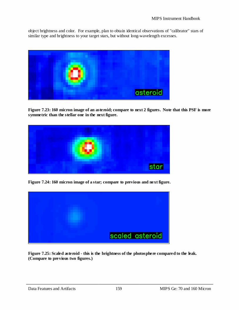
MIPS Instrument Handbook
Data Features and Artifacts 159
MIPS Ge: 70 and 160 Micron
object brightness and color. For example, plan to obtain identical observations of ''calibrator'' stars of similar type and brightness to your target stars, but without long-wavelength excesses.
Figure 7.23: 160 micron image of an asteroid; compare to next 2 figures. Note that this PSF is more symmetric than the stellar one in the next figure.
Figure 7.24: 160 micron image of a star; compare to previous and next figure.
Figure 7.25: Scaled asteroid - this is the brightness of the photosphere compared to the leak. (Compare to previous two figures.)
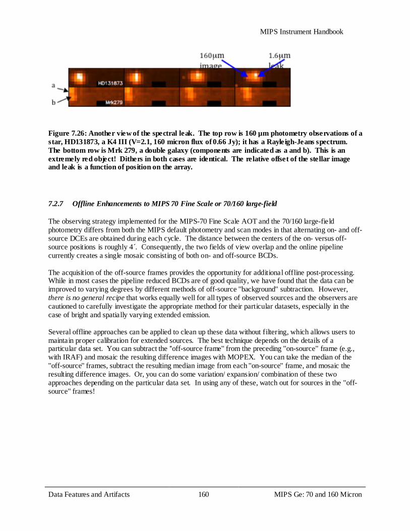
MIPS Instrument Handbook
Data Features and Artifacts 160
MIPS Ge: 70 and 160 Micron
Figure 7.26: Another view of the spectral leak. The top row is 160 µm photometry observations of a star, HD131873, a K4 III (V=2.1, 160 micron flux of 0.66 Jy); it has a Rayleigh-Jeans spectrum. The bottom row is Mrk 279, a double galaxy (components are indicated as a and b). This is an extremely red object! Dithers in both cases are identical. The relative offset of the stellar image and leak is a function of position on the array.
7.2.7 Offline Enhancements to MIPS 70 Fine Scale or 70/160 large-field
The observing strategy implemented for the MIPS-70 Fine Scale AOT and the 70/160 large-field photometry differs from both the MIPS default photometry and scan modes in that alternating on- and off-source DCEs are obtained during each cycle. The distance between the centers of the on- versus off-source positions is roughly 4 .́ Consequently, the two fields of view overlap and the online pipeline currently creates a single mosaic consisting of both on- and off-source BCDs. The acquisition of the off-source frames provides the opportunity for additional offline post-processing. While in most cases the pipeline reduced BCDs are of good quality, we have found that the data can be improved to varying degrees by different methods of off-source ''background'' subtraction. However, there is no general recipe that works equally well for all types of observed sources and the observers are cautioned to carefully investigate the appropriate method for their particular datasets, especially in the case of bright and spatially varying extended emission. Several offline approaches can be applied to clean up these data without filtering, which allows users to maintain proper calibration for extended sources. The best technique depends on the details of a particular data set. You can subtract the ''off-source frame'' from the preceding ''on-source'' frame (e.g., with IRAF) and mosaic the resulting difference images with MOPEX. You can take the median of the ''off-source'' frames, subtract the resulting median image from each ''on-source'' frame, and mosaic the resulting difference images. Or, you can do some variation/ expansion/ combination of these two approaches depending on the particular data set. In using any of these, watch out for sources in the ''off-source'' frames!
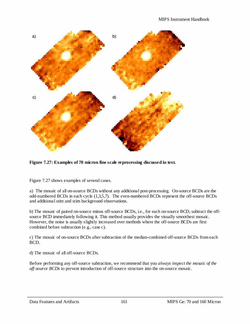
MIPS Instrument Handbook
Data Features and Artifacts 161
MIPS Ge: 70 and 160 Micron
Figure 7.27: Examples of 70 micron fine scale reprocessing discussed in text.
Figure 7.27 shows examples of several cases. a) The mosaic of all on-source BCDs without any additional post-processing. On-source BCDs are the odd-numbered BCDs in each cycle (1,3,5,7). The even-numbered BCDs represent the off-source BCDs and additional stim and stim background observations. b) The mosaic of paired on-source minus off-source BCDs, i.e., for each on-source BCD, subtract the off-source BCD immediately following it. This method usually provides the visually smoothest mosaic. However, the noise is usually slightly increased over methods where the off-source BCDs are first combined before subtraction (e.g., case c). c) The mosaic of on-source BCDs after subtraction of the median-combined off-source BCDs from each BCD. d) The mosaic of all off-source BCDs. Before performing any off-source subtraction, we recommend that you always inspect the mosaic of the off-source BCDs to prevent introduction of off-source structure into the on-source mosaic.
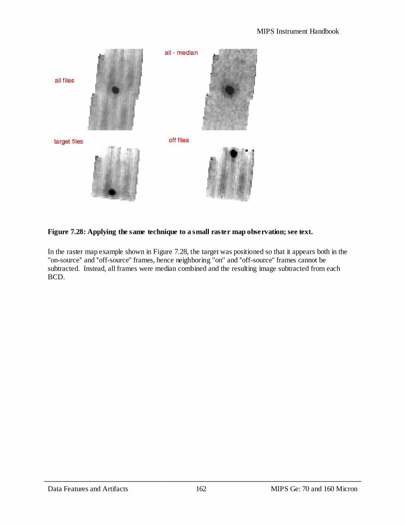
MIPS Instrument Handbook
Data Features and Artifacts 162
MIPS Ge: 70 and 160 Micron
Figure 7.28: Applying the same technique to a small raster map observation; see text. In the raster map example shown in Figure 7.28, the target was positioned so that it appears both in the ''on-source'' and ''off-source'' frames, hence neighboring ''on'' and ''off-source'' frames cannot be subtracted. Instead, all frames were median combined and the resulting image subtracted from each BCD.

MIPS Instrument Handbook
Introduction to Data Analysis 163
24 Micron Data
Chapter 8 Introduction to Data Analysis
8.1 24 Micron Data
8.1.1 Overview and recommended steps for looking at your data
Generally speaking, the 24 micron data is well behaved and the pipeline reduction produces a final product with few artifacts. This means that the default pipeline Level 2 post-BCD 24 micron mosaics can, in many cases, be used for detailed analysis, although some care should still be taken. For instance, the 24 µm pipeline does not correct for latent images, and although it flags cosmic rays, it does not correct for them. It is also common to find a gradient in the background, which in some cases is zodiacal light, while in others it appears to be due to scattered light changing as a function of scan mirror position. To completely remove all these artifacts requires further data reduction. The basic steps to begin data reduction of 24 µm data are the following:
1. Check the online default Level 2 post-BCD mosaics (*maic.fits). a. If this maic.fits file is ok, then you are done and can begin your analysis, although it is still useful
to check the results by remaking the mosaic offline. b. If this maic.fits file shows latents (dark or bright), low-level jailbars, or gradients then you most
likely need to generate your own mosaic.
2. Self-calibrate your data (see section 8.1.2) and re-make the mosaic using MOPEX using Overlap
correction. This step often solves most of the remaining artifact issues. Be sure to use the EBCDs that became available in pipeline S18.12 for photometric observations, which should also remove most of the remaining mirror spots.
3. If a gradient still exists in your final image that you would like removed, you may need to do a sky background removal (see section 8.1.3). Re-make mosaic using MOPEX.
There are certainly a handful observations of extreme complexity that could require a more sophisticated data reduction than presented here in this basic overview, like, for instance, a field with a great deal of extended saturation. However in most cases, these three steps will be all that is required to produce science quality data.
8.1.2 Self-calibration
To correct persistent effects, including long-term latents, low-level jailbars, and gradients, you should use your own data to self-calibrate. First, assemble a list of BCDs without the very bright sources but with the persistent effects. If the latents are caused by your own data, make sure to separate BCDs before and after the offending bright sources. For some data sets, you may want to include the non-prime BCDs.
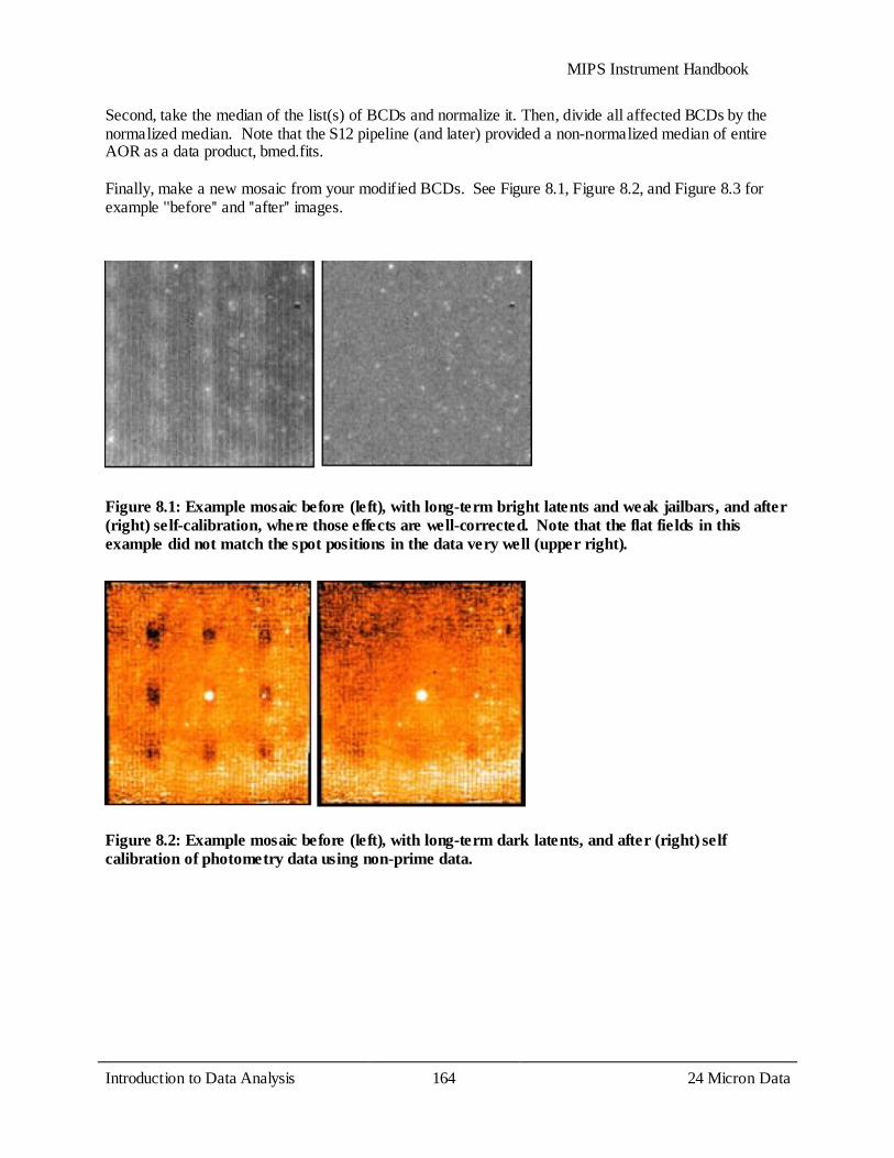
MIPS Instrument Handbook
Introduction to Data Analysis 164
24 Micron Data
Second, take the median of the list(s) of BCDs and normalize it. Then, divide all affected BCDs by the normalized median. Note that the S12 pipeline (and later) provided a non-normalized median of entire AOR as a data product, bmed.fits. Finally, make a new mosaic from your modified BCDs. See Figure 8.1, Figure 8.2, and Figure 8.3 for example ''before'' and ''after'' images.
Figure 8.1: Example mosaic before (left), with long-term bright latents and weak jailbars, and after (right) self-calibration, where those effects are well-corrected. Note that the flat fields in this example did not match the spot positions in the data very well (upper right).
Figure 8.2: Example mosaic before (left), with long-term dark latents, and after (right) self calibration of photometry data using non-prime data.
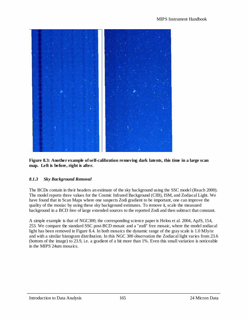
MIPS Instrument Handbook
Introduction to Data Analysis 165
24 Micron Data
Figure 8.3: Another example of self-calibration removing dark latents, this time in a large scan map. Left is before, right is after.
8.1.3 Sky Background Removal
The BCDs contain in their headers an estimate of the sky background using the SSC model (Reach 2000). The model reports three values for the Cosmic Infrared Background (CIB), ISM, and Zodiacal Light. We have found that in Scan Maps where one suspects Zodi gradient to be important, one can improve the quality of the mosiac by using these sky background estimates. To remove it, scale the measured background in a BCD free of large extended sources to the reported Zodi and then subtract that constant. A simple example is that of NGC300; the corresponding science paper is Helou et al. 2004, ApJS, 154, 253. We compare the standard SSC post-BCD mosaic and a ''zodi'' free mosaic, where the model zodiacal light has been removed in Figure 8.4. In both mosaics the dynamic range of the gray scale is 1.0 MJy/sr and with a similar histogram distribution. In this NGC 300 observation the Zodiacal light varies from 23.6 (bottom of the image) to 23.9, i.e. a gradient of a bit more than 1%. Even this small variation is noticeable in the MIPS 24um mosaics.
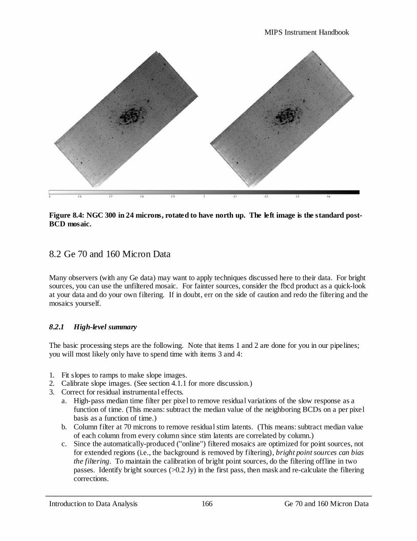
MIPS Instrument Handbook
Introduction to Data Analysis 166
Ge 70 and 160 Micron Data
Figure 8.4: NGC 300 in 24 microns, rotated to have north up. The left image is the standard post-BCD mosaic.
8.2 Ge 70 and 160 Micron Data
Many observers (with any Ge data) may want to apply techniques discussed here to their data. For bright sources, you can use the unfiltered mosaic. For fainter sources, consider the fbcd product as a quick-look at your data and do your own filtering. If in doubt, err on the side of caution and redo the filtering and the mosaics yourself.
8.2.1 High-level summary
The basic processing steps are the following. Note that items 1 and 2 are done for you in our pipelines; you will most likely only have to spend time with items 3 and 4:
1. Fit slopes to ramps to make slope images. 2. Calibrate slope images. (See section 4.1.1 for more discussion.) 3. Correct for residual instrumental effects.
a. High-pass median time filter per pixel to remove residual variations of the slow response as a function of time. (This means: subtract the median value of the neighboring BCDs on a per pixel basis as a function of time.)
b. Column filter at 70 microns to remove residual stim latents. (This means: subtract median value of each column from every column since stim latents are correlated by column.)
c. Since the automatically-produced (''online'') filtered mosaics are optimized for point sources, not for extended regions (i.e., the background is removed by filtering), bright point sources can bias the filtering. To maintain the calibration of bright point sources, do the filtering offline in two passes. Identify bright sources (>0.2 Jy) in the first pass, then mask and re-calculate the filtering corrections.

MIPS Instrument Handbook
Introduction to Data Analysis 167
Ge 70 and 160 Micron Data
4. Co-add images to make mosaics. (Can be done entirely with MOPEX.) a. Correct for array distortion. b. Interpolation of frames onto fiducial sky frame. c. Outlier rejection based on redundancy. d. Re-interpolation of frames. e. Coadd final frames.
8.2.2 Point vs. extended sources, or why there are 2 BCDs
The goal of BCD pipeline processing is to produce the best possible data products that can be derived from automated processing. Currently, the SSC produces two BCD products: (1) bcd.fits which is the standard calibrated BCD and (2) fbcd.fits which is a ''filtered'' bcd product designed for point sources. The fbcd is produced by subtracting off a median of the surrounding DCEs as a function of time per pixel. This filtering technique significantly mitigates the accumulation of stimflash latents and the residual background drifts due to variations of the slow response as a function of time (see below for more information). The application of the median filter removes the background from both the sky and the residual detector effects (i.e., loses information about the extended background level in the field). Early tests show that the application of a median filter maintains point source calibration for scan maps of fields with uniform backgrounds, but the fbcds do not preserve calibration for extended sources or for bright (>0.2 Jy) point sources within complex emission regions. For extended and/or bright sources, you may achieve better results with offline custom filtering using the GeRT (see section 8.2.3). A mosaic constructed from some sample unfiltered MIPS-70 scan map data appears in Figure 7.20; a mosaic constructed from the same data but filtered is in Figure 8.5. The dark horizontal (in-scan) stripes are fast/slow response variations, which are removed from the data using a temporal median filter per pixel in the current automatic pipeline. The bright vertical stripes are stim latents, which are removed in the pipeline using column median filtering. These sample FLS data date from early in the mission, e.g. they were taken with the old bias settings (see ''stim latents'' below). Most data were taken with the new bias setting, so the magnitude of both of these effects should be lessened in a typical observation. Figure 8.6 shows a flowchart of possible analysis steps, discussed in much more detail below. To the BCD level, our pipelines yield quantitatively similar results to those described in Gordon et al. (2005, PASP, 117, 503). Real-life specific examples of extended source work with MIPS can be found, for example, in the ApJS special issue; see, e.g., the paper by Engelbracht et al. (2004, ApJS, 154, 248) on NGC 55, Helou et al. (2004, ApJS, 154, 253) on NGC 300, and/or Regan et al. (2004, ApJS, 154, 204) on NGC 7331.
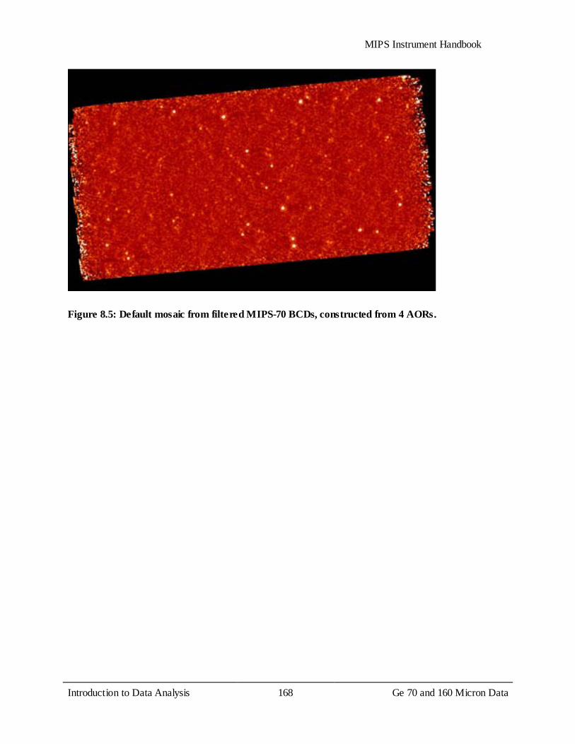
MIPS Instrument Handbook
Introduction to Data Analysis 168
Ge 70 and 160 Micron Data
Figure 8.5: Default mosaic from filtered MIPS-70 BCDs, constructed from 4 AORs.
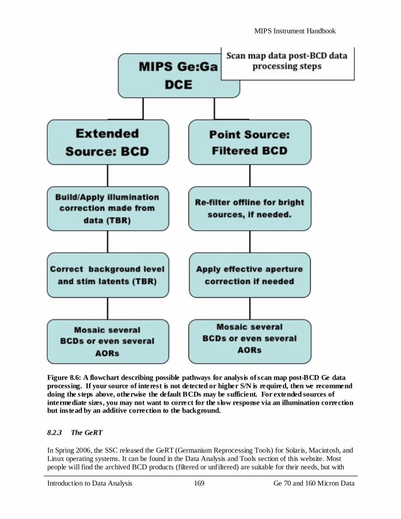
MIPS Instrument Handbook
Introduction to Data Analysis 169
Ge 70 and 160 Micron Data
Figure 8.6: A flowchart describing possible pathways for analysis of scan map post-BCD Ge data processing. If your source of interest is not detected or higher S/N is required, then we recommend doing the steps above, otherwise the default BCDs may be sufficient. For extended sources of intermediate sizes, you may not want to correct for the slow response via an illumination correction but instead by an additive correction to the background.
8.2.3 The GeRT
In Spring 2006, the SSC released the GeRT (Germanium Reprocessing Tools) for Solaris, Macintosh, and Linux operating systems. It can be found in the Data Analysis and Tools section of this website. Most people will find the archived BCD products (filtered or unfiltered) are suitable for their needs, but with

MIPS Instrument Handbook
Introduction to Data Analysis 170
Ge 70 and 160 Micron Data
the GeRT, you can either ''clean up'' the BCDs, or reprocess the raw data. Examples of cases in which reprocessing from scratch would be important include the following: (a) the online stim calibration was not done optimally, e.g., extrapolated stim calibration or stim calibration corrupted by bright emission regions; (b) important new or updated calibration files and/or pipeline corrections not yet available online but important for a specific case; (c) optimization of the pipeline parameters for non-standard data and/or specific science applications for expert users.
8.2.4 Recommended steps for looking at your data
1. Using the BCDs, look at the online default post-BCD mosaics (*maic.fits, used to be *msaic.fits). a. If this maic.fits file is ok, then you're done, although it is still useful to check the results by
remaking the mosaic offline. b. If this maic.fits file has bad outlier rejection, remake the mosaic from the online BCDs (using
MOPEX). c. If this maic.fits file has streaks/artifacts, then check the filtered mosaic (*mfilt.fits).
2. Look at the online filtered mosaic (*mfilt.fits), which was constructed from the filtered (*fbcd.fits)
files. a. If this mfilt.fits file has bad outlier rejection, remake the mosaic from the online *fbcd.fits files
(using MOPEX). b. If this mfilt.fits file has negative sidelobes, do 2-pass filtering offline starting with the BCDs and
adjust the filtering parameters based on the extent of the source.
3. If stim response artifacts are present due to bright sources, then reprocess from scratch (the ''raw''
data) yourself using the GeRT and make new BCDs by masking out bad stim frames/pixels. You should correct for any multiplicative stim-response effects first and then correct for the residual additive slow response drifts via filtering.
The choice of filtered vs. unfiltered BCDs depends on the your scientific goals. Extended absolute background measurements should be made from the unfiltered BCDs. For point sources and small extended regions, you can use filtered products (optimized for your source, if necessary). Saturated data close to the saturation limit could potentially be recovered by changing the pipeline parameters for slope determination. Note, however, that this will affect absolute flux calibration.
8.2.5 Note on point source photometry
Since the small field photometry AOTs do not dither with offsets much larger than the size of the MIPS-Ge PSF, temporally filtered fbcd data will underestimate the true point source flux values (by roughly about 10%). We recommend that you mosaic both the filtered and non-filtered data to determine whether or not additional offline processing is needed. You may find that the offline techniques described here significantly improve your data products. To maintain point source calibration, it's possible to mask out the point sources before filtering. If you don't do that, we recommend that you measure the point sources before and after filtering to check its impact on the flux calibration.
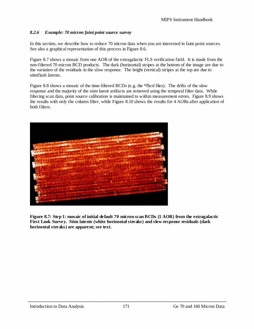
MIPS Instrument Handbook
Introduction to Data Analysis 171
Ge 70 and 160 Micron Data
8.2.6 Example: 70 micron faint point source survey
In this section, we describe how to reduce 70 micron data when you are interested in faint point sources. See also a graphical representation of this process in Figure 8.6. Figure 8.7 shows a mosaic from one AOR of the extragalactic FLS verification field. It is made from the non-filtered 70 micron BCD products. The dark (horizontal) stripes at the bottom of the image are due to the variation of the residuals in the slow response. The bright (vertical) stripes at the top are due to stimflash latents. Figure 8.8 shows a mosaic of the time-filtered BCDs (e.g. the *fbcd files). The drifts of the slow response and the majority of the stim latent artifacts are removed using the temporal filter data. While filtering scan data, point source calibration is maintained to within measurement errors. Figure 8.9 shows the results with only the column filter, while Figure 8.10 shows the results for 4 AORs after application of both filters.
Figure 8.7: Step 1: mosaic of initial default 70 micron scan BCDs (1 AOR) from the extragalactic First Look Survey. Stim latents (white horizontal streaks) and slow response residuals (dark horizontal streaks) are apparent; see text.
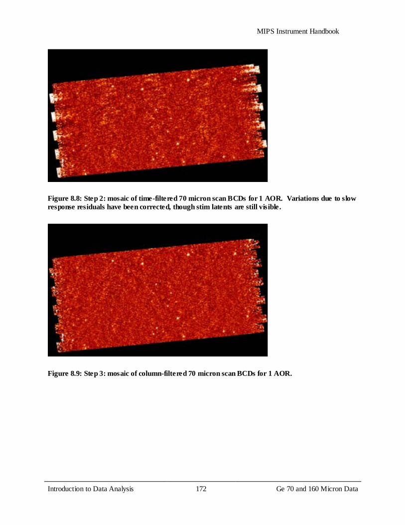
MIPS Instrument Handbook
Introduction to Data Analysis 172
Ge 70 and 160 Micron Data
Figure 8.8: Step 2: mosaic of time-filtered 70 micron scan BCDs for 1 AOR. Variations due to slow response residuals have been corrected, though stim latents are still visible.
Figure 8.9: Step 3: mosaic of column-filtered 70 micron scan BCDs for 1 AOR.
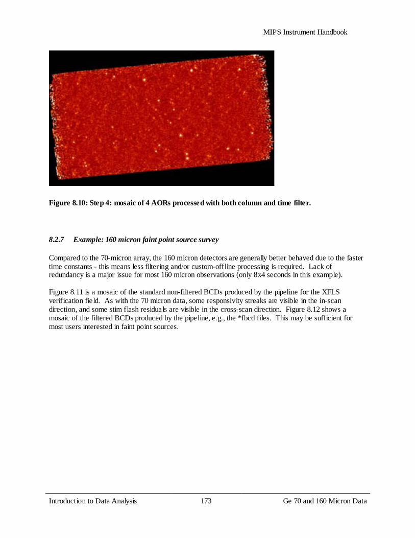
MIPS Instrument Handbook
Introduction to Data Analysis 173
Ge 70 and 160 Micron Data
Figure 8.10: Step 4: mosaic of 4 AORs processed with both column and time filter.
8.2.7 Example: 160 micron faint point source survey
Compared to the 70-micron array, the 160 micron detectors are generally better behaved due to the faster time constants - this means less filtering and/or custom-offline processing is required. Lack of redundancy is a major issue for most 160 micron observations (only 8x4 seconds in this example). Figure 8.11 is a mosaic of the standard non-filtered BCDs produced by the pipeline for the XFLS verification field. As with the 70 micron data, some responsivity streaks are visible in the in-scan direction, and some stim flash residuals are visible in the cross-scan direction. Figure 8.12 shows a mosaic of the filtered BCDs produced by the pipeline, e.g., the *fbcd files. This may be sufficient for most users interested in faint point sources.
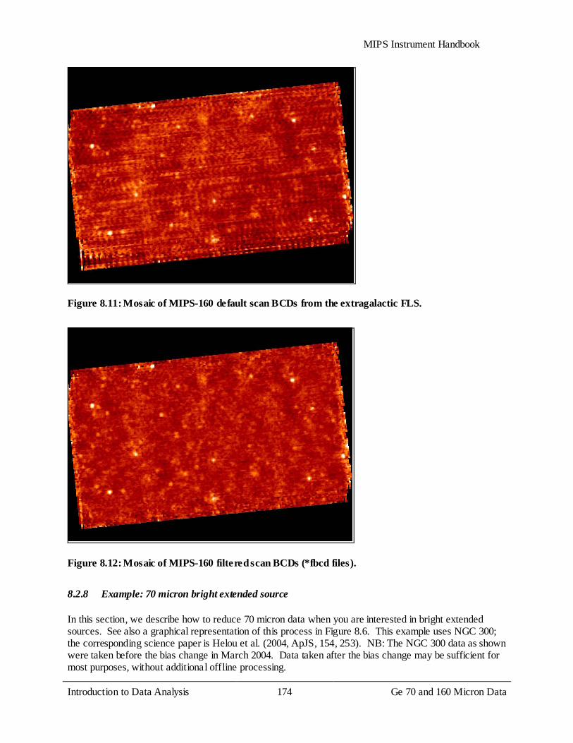
MIPS Instrument Handbook
Introduction to Data Analysis 174
Ge 70 and 160 Micron Data
Figure 8.11: Mosaic of MIPS-160 default scan BCDs from the extragalactic FLS.
Figure 8.12: Mosaic of MIPS-160 filtered scan BCDs (*fbcd files).
8.2.8 Example: 70 micron bright extended source
In this section, we describe how to reduce 70 micron data when you are interested in bright extended sources. See also a graphical representation of this process in Figure 8.6. This example uses NGC 300; the corresponding science paper is Helou et al. (2004, ApJS, 154, 253). NB: The NGC 300 data as shown were taken before the bias change in March 2004. Data taken after the bias change may be sufficient for most purposes, without additional offline processing.
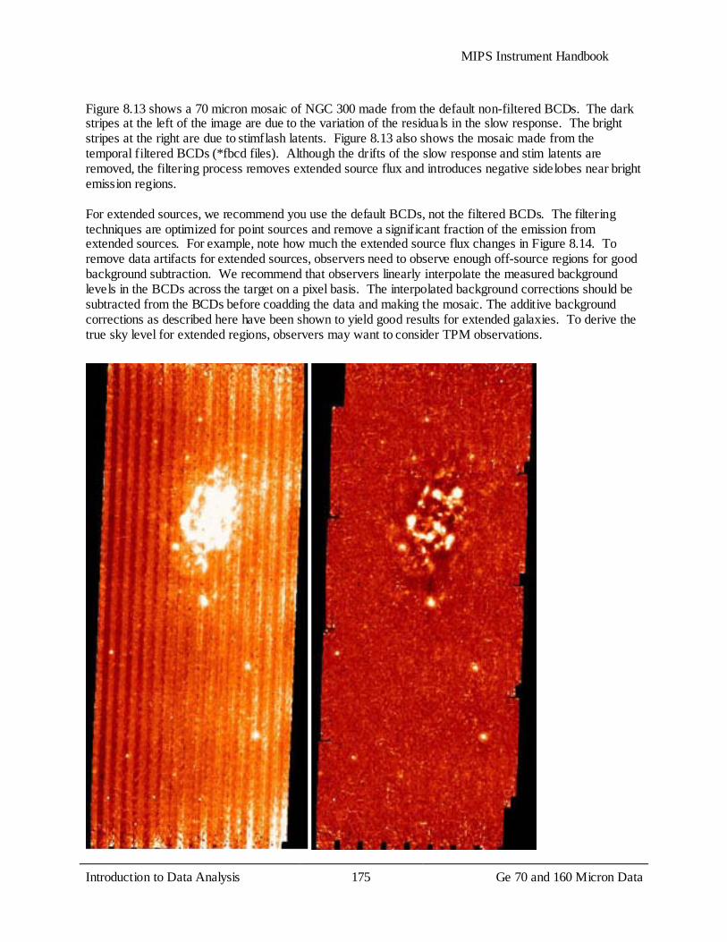
MIPS Instrument Handbook
Introduction to Data Analysis 175
Ge 70 and 160 Micron Data
Figure 8.13 shows a 70 micron mosaic of NGC 300 made from the default non-filtered BCDs. The dark stripes at the left of the image are due to the variation of the residuals in the slow response. The bright stripes at the right are due to stimflash latents. Figure 8.13 also shows the mosaic made from the temporal filtered BCDs (*fbcd files). Although the drifts of the slow response and stim latents are removed, the filtering process removes extended source flux and introduces negative sidelobes near bright emission regions. For extended sources, we recommend you use the default BCDs, not the filtered BCDs. The filtering techniques are optimized for point sources and remove a significant fraction of the emission from extended sources. For example, note how much the extended source flux changes in Figure 8.14. To remove data artifacts for extended sources, observers need to observe enough off-source regions for good background subtraction. We recommend that observers linearly interpolate the measured background levels in the BCDs across the target on a pixel basis. The interpolated background corrections should be subtracted from the BCDs before coadding the data and making the mosaic. The additive background corrections as described here have been shown to yield good results for extended galaxies. To derive the true sky level for extended regions, observers may want to consider TPM observations.
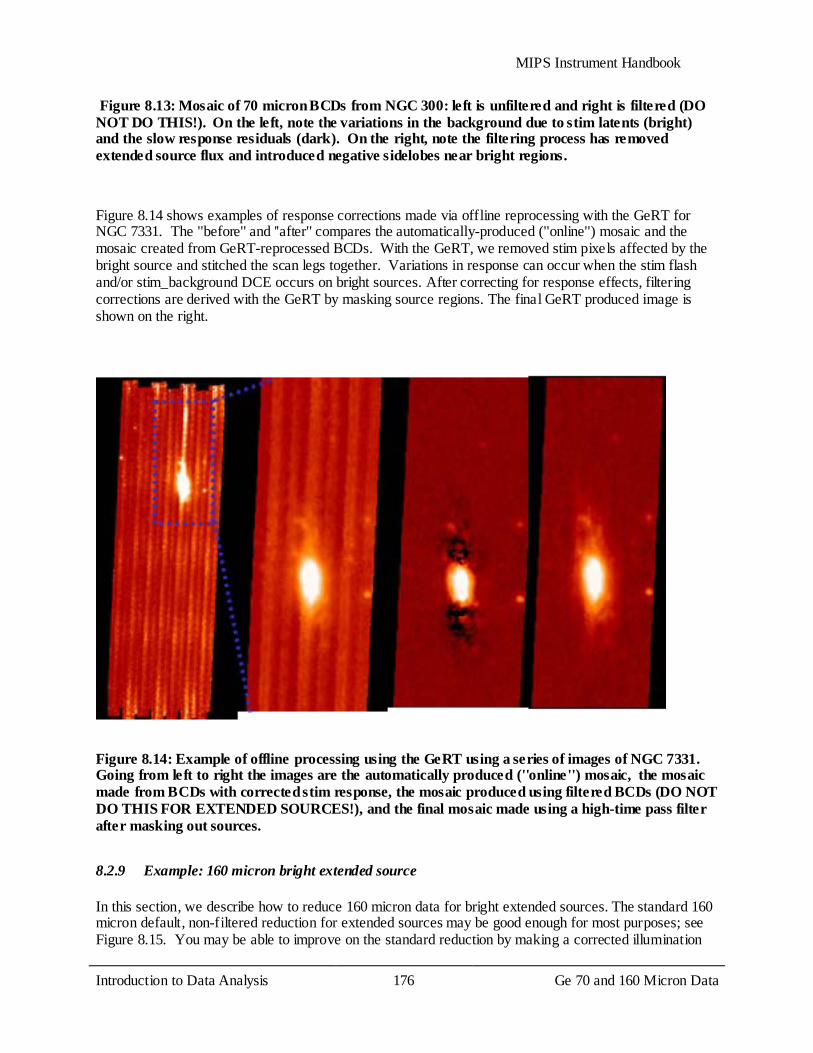
MIPS Instrument Handbook
Introduction to Data Analysis 176
Ge 70 and 160 Micron Data
Figure 8.13: Mosaic of 70 micron BCDs from NGC 300: left is unfiltered and right is filtered (DO NOT DO THIS!). On the left, note the variations in the background due to stim latents (bright) and the slow response residuals (dark). On the right, note the filtering process has removed extended source flux and introduced negative sidelobes near bright regions.
Figure 8.14 shows examples of response corrections made via offline reprocessing with the GeRT for NGC 7331. The ''before'' and ''after'' compares the automatically-produced (''online'') mosaic and the mosaic created from GeRT-reprocessed BCDs. With the GeRT, we removed stim pixels affected by the bright source and stitched the scan legs together. Variations in response can occur when the stim flash and/or stim_background DCE occurs on bright sources. After correcting for response effects, filtering corrections are derived with the GeRT by masking source regions. The final GeRT produced image is shown on the right.
Figure 8.14: Example of offline processing using the GeRT using a series of images of NGC 7331. Going from left to right the images are the automatically produced (''online'') mosaic, the mosaic made from BCDs with corrected stim response, the mosaic produced using filtered BCDs (DO NOT DO THIS FOR EXTENDED SOURCES!), and the final mosaic made using a high-time pass filter after masking out sources.
8.2.9 Example: 160 micron bright extended source
In this section, we describe how to reduce 160 micron data for bright extended sources. The standard 160 micron default, non-filtered reduction for extended sources may be good enough for most purposes; see Figure 8.15. You may be able to improve on the standard reduction by making a corrected illumination

MIPS Instrument Handbook
Introduction to Data Analysis 177
Ge 70 and 160 Micron Data
correction file from the data themselves and applying the correction before mosaicking. If the DCE after the stim is significantly brighter than following BCDs, you may not want to include this DCE in the mosaic, depending on the level of redundancy in the data set. The use of median filtered data is not recommended for extended sources at 160 microns; see Figure 8.15. A second example of a galactic object (the cluster L1228) on a bright background appears in Figure 8.16 through Figure 8.18. Again, constructing a mosaic from the filtered BCDs is not recommended.
Figure 8.15: Mosaic of unfiltered (left) and filtered (right; DO NOT DO THIS!) 160 micron scan BCDs of NGC 300. On the left, the dark and bright ''dotted lines'' are due to bad stim-subtracted solutions for some pixels due to the bright object. Note on the right among other things the dark sidelobes introduced by the filtering. See text.
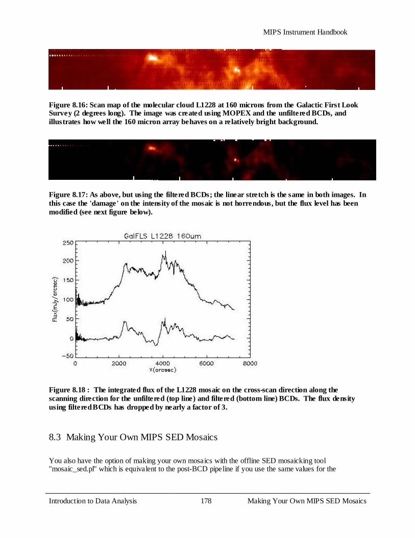
MIPS Instrument Handbook
Introduction to Data Analysis 178
Making Your Own MIPS SED Mosaics
Figure 8.16: Scan map of the molecular cloud L1228 at 160 microns from the Galactic First Look Survey (2 degrees long). The image was created using MOPEX and the unfiltered BCDs, and illustrates how well the 160 micron array behaves on a relatively bright background.
Figure 8.17: As above, but using the filtered BCDs; the linear stretch is the same in both images. In this case the 'damage' on the intensity of the mosaic is not horrendous, but the flux level has been modified (see next figure below).
Figure 8.18 : The integrated flux of the L1228 mosaic on the cross-scan direction along the scanning direction for the unfiltered (top line) and filtered (bottom line) BCDs. The flux density using filtered BCDs has dropped by nearly a factor of 3.
8.3 Making Your Own MIPS SED Mosaics
You also have the option of making your own mosaics with the offline SED mosaicking tool ''mosaic_sed.pl'' which is equivalent to the post-BCD pipeline if you use the same values for the

MIPS Instrument Handbook
Introduction to Data Analysis 179
Making Your Own MIPS SED Mosaics
controlling parameters as the pipeline. The tool is a part of the MOPEX package and is downloadable from the website. There may be some advantages to doing your own mosaics. For example, you can do further data manipulation at the BCD level before mosaicking; you can also use a different interpolation option than the default one. If you have a raster map you can use this offline tool to produce a big mosaic using all the raster points. The program uses a NameList file as an input. In this file you specify lists of image to process and where the results should be output. The instructions on this NameList file as well as how to set up and run this program are given in the MOPEX document on ''mosaic_sed.pl''.

MIPS Instrument Handbook
Introduction to Data Analysis 180
Making Your Own MIPS SED Mosaics
Appendix A. Version Log Version 3.0, March 2011:
Some very minor updates to text and headings for better clarity and readability. Added more references to Level 1 (BCD) and Level 2 (post-BCD) data for clearer connection to data products delivered by the Spitzer Heritage Archive. Made minor corrections to listed MIPS zero points and their errors. Added mention of S18.13 pipeline label to pipeline history log. It is identical to S18.12. Removed references to obsolete software LEOPARD in favor or the Spitzer Heritage Archive.
Version 2.0, September 2010: The data products list in Chapter 6 was updated to include a description of all files being delivered
by the Spitzer Heritage Archive. Descriptions of files not delivered were removed. Minor corrections made on labeling of RAW vs. BCD products.
A history of pipeline changes of conversion factors (DN to MJy) was added to section 4.3.2. Fixed incorrect conversion factor reference that remained in text (not in table). Update/corrections to bit mask tables in section 6.5. Additional text describing fatal bits rejected by default MOPEX mosaic pipeline added.
Some additional KEYWORD descriptions added to Header Keywords, section 6.6. Improvement in legibility of several figures (Figures 2.14, 2.15, 3.17, 3.18).
Added version log appendix and lists of Tables and Figures.
Version 1.0, February 2010:
The first version of the MIPS instrument Handbook, which includes information from the MIPS Data Handbook, the Cryogenic Spitzer Observer’s Manual, and Spitzer Science Center webpages.

MIPS Instrument Handbook
Introduction to Data Analysis 181
Making Your Own MIPS SED Mosaics
Appendix B. Acronyms Table A.1: Acronyms used in this manual.
ADC Analog to Digital Converter
ADU Analog to Digital Units
AOR Astronomical Observation Request(s)
AOT Astronomical Observation Template(s)
BCD Basic Calibrated Data
BIB Blocked Impurity Band
C&DH Command and Data Handling
CA Cryogenic Assembly
CE Combined Electronics
CIB Cold Interface Board
CMOS Complementary Metal-Oxide Semiconductor
CP Call for Proposals
CR Cosmic Ray
CSE Control Section Electronics
CSFS Control Section Flight Software
CSMM Cryogenic Scan Mirror Mechanism (MIPS scan mirror)
CTA Cryogenic Telescope Assembly
CTIA Capacitive TransImpedence Amplifier
DAC Digital to Analog Converter
DCE Data Collection Event
DCS Double Correlated Sampling
Dec Declination
DN Data Number

MIPS Instrument Handbook
Introduction to Data Analysis 182
Making Your Own MIPS SED Mosaics
DQE Detector Quantum Efficiency
DSN Deep Space Network
EDAC Error Detection and Correction
EEPROM Electrically Erasable Programmable Read Only Memory
FAQ Frequently Asked Question
FITS Flexible Image Transport System
FLS First Look Survey
FOV Field-of-View
FPA Focal Plane Array
FPMA Focal Plane Mount Array
FWHM Full Width at Half Maximum
GSFC Goddard Space Flight Center
GO General Observer(s)
GTO Guaranteed Time Observer(s)
HGA High Gain Antenna
HST Hubble Space Telescope
IBC Impurity Band Conduction
ICRS International Celestial Reference System
IER Instrument Engineering Request - like an AOR, but for specific engineering tasks not able to be accomplished using an AOR.
IOC In-Orbit Check out
IPAC Infrared Processing and Analysis Center
IR Infrared
IRAC InfraRed Array Camera
IRAS InfraRed Astronomical Satellite
IRS InfraRed Spectrograph
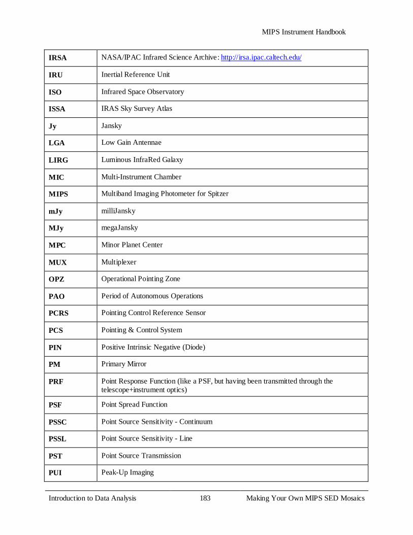
MIPS Instrument Handbook
Introduction to Data Analysis 183
Making Your Own MIPS SED Mosaics
IRSA NASA/IPAC Infrared Science Archive: http://irsa.ipac.caltech.edu/
IRU Inertial Reference Unit
ISO Infrared Space Observatory
ISSA IRAS Sky Survey Atlas
Jy Jansky
LGA Low Gain Antennae
LIRG Luminous InfraRed Galaxy
MIC Multi-Instrument Chamber
MIPS Multiband Imaging Photometer for Spitzer
mJy milliJansky
MJy megaJansky
MPC Minor Planet Center
MUX Multiplexer
OPZ Operational Pointing Zone
PAO Period of Autonomous Operations
PCRS Pointing Control Reference Sensor
PCS Pointing & Control System
PIN Positive Intrinsic Negative (Diode)
PM Primary Mirror
PRF Point Response Function (like a PSF, but having been transmitted through the telescope+instrument optics)
PSF Point Spread Function
PSSC Point Source Sensitivity - Continuum
PSSL Point Source Sensitivity - Line
PST Point Source Transmission
PUI Peak-Up Imaging
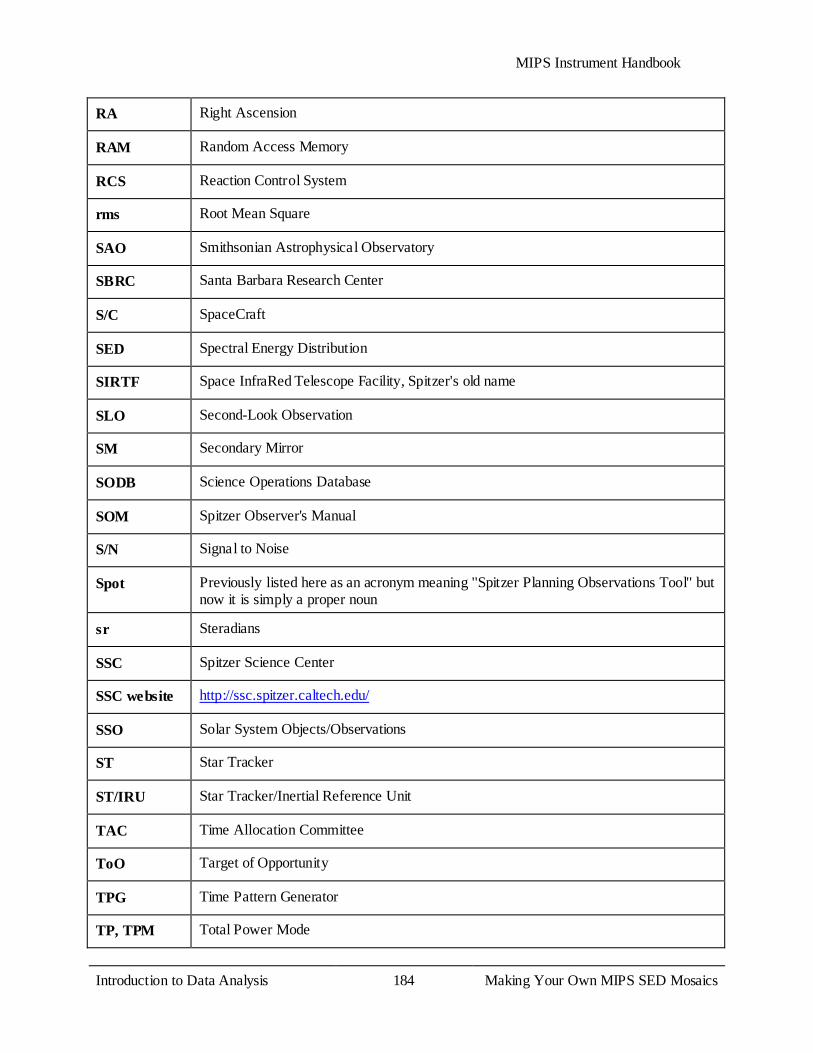
MIPS Instrument Handbook
Introduction to Data Analysis 184
Making Your Own MIPS SED Mosaics
RA Right Ascension
RAM Random Access Memory
RCS Reaction Control System
rms Root Mean Square
SAO Smithsonian Astrophysical Observatory
SBRC Santa Barbara Research Center
S/C SpaceCraft
SED Spectral Energy Distribution
SIRTF Space InfraRed Telescope Facility, Spitzer's old name
SLO Second-Look Observation
SM Secondary Mirror
SODB Science Operations Database
SOM Spitzer Observer's Manual
S/N Signal to Noise
Spot Previously listed here as an acronym meaning ''Spitzer Planning Observations Tool'' but now it is simply a proper noun
sr Steradians
SSC Spitzer Science Center
SSC website http://ssc.spitzer.caltech.edu/
SSO Solar System Objects/Observations
ST Star Tracker
ST/IRU Star Tracker/Inertial Reference Unit
TAC Time Allocation Committee
ToO Target of Opportunity
TPG Time Pattern Generator
TP, TPM Total Power Mode

MIPS Instrument Handbook
Introduction to Data Analysis 185
Making Your Own MIPS SED Mosaics
QE Quantum Efficiency
WASS Wide Angle Sun Sensor
WEA Warm Electronics Assembly
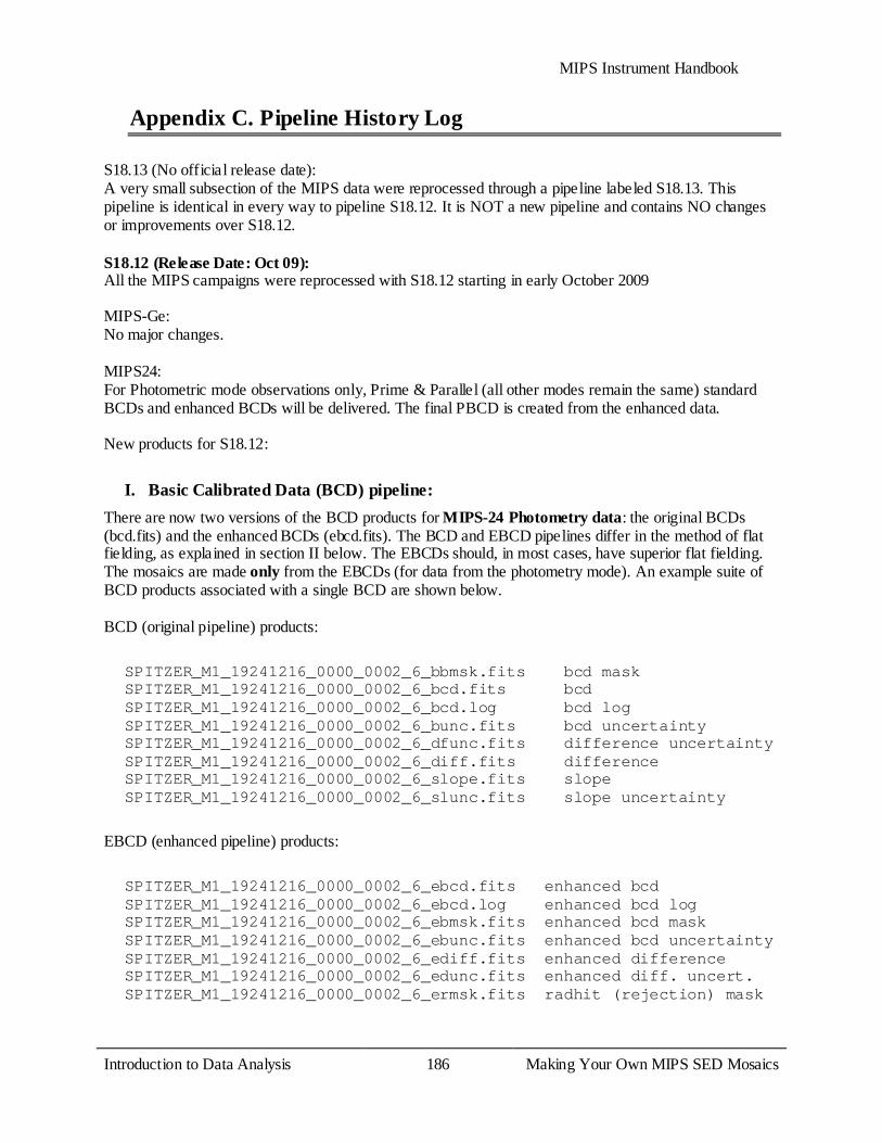
MIPS Instrument Handbook
Introduction to Data Analysis 186
Making Your Own MIPS SED Mosaics
Appendix C. Pipeline History Log S18.13 (No official release date): A very small subsection of the MIPS data were reprocessed through a pipeline labeled S18.13. This pipeline is identical in every way to pipeline S18.12. It is NOT a new pipeline and contains NO changes or improvements over S18.12. S18.12 (Release Date: Oct 09): All the MIPS campaigns were reprocessed with S18.12 starting in early October 2009 MIPS-Ge: No major changes. MIPS24: For Photometric mode observations only, Prime & Parallel (all other modes remain the same) standard BCDs and enhanced BCDs will be delivered. The final PBCD is created from the enhanced data. New products for S18.12:
I. Basic Calibrated Data (BCD) pipeline: There are now two versions of the BCD products for MIPS-24 Photometry data: the original BCDs (bcd.fits) and the enhanced BCDs (ebcd.fits). The BCD and EBCD pipelines differ in the method of flat fielding, as explained in section II below. The EBCDs should, in most cases, have superior flat fielding. The mosaics are made only from the EBCDs (for data from the photometry mode). An example suite of BCD products associated with a single BCD are shown below. BCD (original pipeline) products:
SPITZER_M1_19241216_0000_0002_6_bbmsk.fits bcd mask SPITZER_M1_19241216_0000_0002_6_bcd.fits bcd SPITZER_M1_19241216_0000_0002_6_bcd.log bcd log SPITZER_M1_19241216_0000_0002_6_bunc.fits bcd uncertainty SPITZER_M1_19241216_0000_0002_6_dfunc.fits difference uncertainty SPITZER_M1_19241216_0000_0002_6_diff.fits difference SPITZER_M1_19241216_0000_0002_6_slope.fits slope SPITZER_M1_19241216_0000_0002_6_slunc.fits slope uncertainty
EBCD (enhanced pipeline) products:
SPITZER_M1_19241216_0000_0002_6_ebcd.fits enhanced bcd SPITZER_M1_19241216_0000_0002_6_ebcd.log enhanced bcd log SPITZER_M1_19241216_0000_0002_6_ebmsk.fits enhanced bcd mask SPITZER_M1_19241216_0000_0002_6_ebunc.fits enhanced bcd uncertainty SPITZER_M1_19241216_0000_0002_6_ediff.fits enhanced difference SPITZER_M1_19241216_0000_0002_6_edunc.fits enhanced diff. uncert. SPITZER_M1_19241216_0000_0002_6_ermsk.fits radhit (rejection) mask
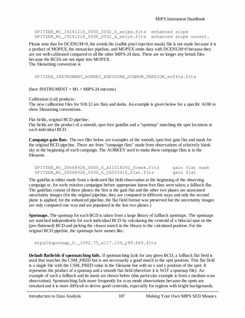
MIPS Instrument Handbook
Introduction to Data Analysis 187
Making Your Own MIPS SED Mosaics
SPITZER_M1_19241216_0000_0002_6_eslpe.fits enhanced slope SPITZER_M1_19241216_0000_0002_6_eslun.fits enhanced slope uncert.
Please note that for DCENUM=0, the ersmk.fits (radhit pixel rejection mask) file is not made because it is a product of MOPEX, the mosaicker pipeline, and MOPEX omits data with DCENUM=0 because they are not well-calibrated compared to all the other MIPS-24 data. There are no longer any brmsk files because the BCDs are not input into MOPEX. The filenaming convention is
SPITZER_INSTRUMENT_AORKEY_EXPOSURE_DCENUM_VERSION_suffix.fits
(here INSTRUMENT = M1 = MIPS-24 microns) Calibration (cal) products: The new calibration files for S18.12 are flats and darks. An example is given below for a specific AOR to show filenaming conventions. Flat fields, original BCD pipeline: Flat fields are the product of a smooth, spot-free gainflat and a ''spotmap'' matching the spot locations in each individual BCD. Campaign gain flats . The two files below are examples of the smooth, spot-free gain flat and mask for the original BCD pipeline. These are from ''campaign flats'' made from observations of relatively blank sky at the beginning of each campaign. The AORKEY used to make these campaign flats is in the filename.
SPITZER_M1_20668928_0000_6_A31018392_fcmsk.fits gain flat mask SPITZER_M1_20668928_0000_6_C6025416_flat.fits gain flat
The gainflat is either made from a dedicated flat field observation at the beginning of the observing campaign or, for early mission campaigns before appropriate latent-free flats were taken, a fallback flat. The gainflats consist of three planes: the first is the gain flat and the other two planes are associated uncertainty images (for the original pipeline, they are computed in different ways and only the second plane is applied; for the enhanced pipeline, the flat field format was preserved but the uncertainty images are only computed one way and are populated in the last two planes.) Spotmaps. The spotmap for each BCD is taken from a large library of fallback spotmaps. The spotmaps are matched independently for each individual BCD by calculating the centroid of a fiducial spot on the (pre-flattened) BCD and picking the closest match in the library to the calculated position. For the original BCD pipeline, the spotmaps have names like:
mips24spotmap_0._1992.75_x117.159_y99.849.fits
Default flatfields if spotmatching fails. If spotmatching fails for any given BCD, a fallback flat field is used that matches the CSM_PRED but is not necessarily a good match to the spot position. This flat field is a single file with the CSM_PRED value in the filename but with no x and y position of the spot. It represents the product of a spotmap and a smooth flat field (therefore it is NOT a spotmap file). An example of such a fallback and its mask are shown below (this particular example is from a medium scan observation). Spotmatching fails more frequently for scan mode observations because the spots are streaked and it is more difficult to derive good centroids, especially for regions with bright backgrounds.
MIPS Instrument Handbook
Introduction to Data Analysis 188
Making Your Own MIPS SED Mosaics
mips24_flatfield_6320._1959.5.fits mips24_flatfield_6320._1959.5_cmask.fits
The filename convention for the default flatfield when spotmatching fails is:
mips24_flatfield_SCANRATE_CSM_PRED.fits
II. NEW, Enhanced BCD (EBCD) pipeline.
Flatfields are the product of a smooth, spot-free gainflat and a ''spotflat'' shifted to match the spot locations in each BCD. Here, all of the BCDs in the AOR are used to compute a single spot offset (SPOT_DY) in the y-direction relative to a reference template spotflat file. This single offset shift is applied to all of the planes in the spotflat file. The shifted spotflat file is a cube, matching the spot position of the current AOR, with one plane for each mirror position used in MIPS-24 photometry mode, in ascending order of header keyword CSM_PRED (predicted cryogenic scan mirror position). After shifting the reference to match the current AOR, the appropriate planes are used for flat fielding. The headers of these files have explanatory keywords (COMM1,COMM2, etc.) describing the nature of each file.
SPITZER_M1_19241216_0000_6_A31034185_sfunc.fits spot-flat uncert. SPITZER_M1_19241216_0000_6_A31034187_sfcsm.fits spot-flat CSM_PRED array (1-D array) SPITZER_M1_19241216_0000_6_A31034188_gfmsk.fits gain flat mask SPITZER_M1_19241216_0000_6_A31034189_gflat.fits gain flat (spot- free, from campaign flat SPITZER_M1_19241216_0000_6_C6027630_sflat.fits shifted spot flat cube
''Extra'' flats for campaigns using fallback rather than campaign gainflats. For the campaigns early in the mission that require fallback flats (due to the fact that no latent-free flat fields were taken during the campaign), a set of additional flat fields appear for both original and enhanced pipelines. These are to be considered ''extra'' files that are currently archived due to how fallback files are retrieved from the database. They can essentially be ignored as they are associated with the unshifted flats and are not actually applied to the EBCDs. They will appear as follows: For the original BCD pipeline:
mips24_flat_090909.fits fallback gain flat for original bcd pipeline mips24_flat_090909_cmask.fits mask for above
For the enhanced pipeline:
mips24_flat_090909_aorgain.fits fallback gain flat mips24_flat_090909_aorgmsk.fits fallback gain flat mask mips24_flat_090909_aorspotcsm.fits fallback CSM_PRED array (1-D array) mips24_flat_090909_aorspotmsk.fits fallback unshifted spot
MIPS Instrument Handbook
Introduction to Data Analysis 189
Making Your Own MIPS SED Mosaics
flat mask mips24_flat_090909_aorspotunc.fits fallback unshifted spot flat uncertainty mips24_flat_090909_aorspotval.fits fallback unshifted spot flat cube
Darks: New dark files were made for S18.12 (Oct. 2009). They are applied to both BCDs and EBCDs. They reflect improved calibration and signal-to-noise (especially for DCENUM> 0) over older verions and were made from approximately 100 dedicated dark observations taken over many campaigns. For MIPS-24, there is no clear evidence that photons are detected in the default scan mirror position used for dark observations; thus, darks derived from the same exposure time observations (10 sec) are applied to all MIPS-24 data, regardless of the exposure time of the science data.
mips24_dark_090804_sur1.fits dark for DCENUM=0 mips24_dark_090804_sur1_cmask.fits dark mask for DCENUM=0 mips24_dark_090804_sur1_uncert.fits dark uncertainty for DCENUM=0 mips24_dark_090804_sur2.fits dark for DCENUM>0 mips24_dark_090804_sur2_cmask.fits dark mask for DCENUM>0 mips24_dark_090804_sur2_uncert.fits dark uncertainty for DCENUM>0
S18.7 (Release Date: Jan 09) BQD: headers for Scan & Photometry include now ZODIMIN = in [MJy/sr] minimum zodiacal background in AOR ZODIMAX = in [MJy/sr] maximum zodiacal background in AOR ZODIMED = in [MJy/sr] median zodaical background in AOR S18.0 (June 08) Header information updated WCS CD matrix keywords were added to the Post-BCD file headers. The CDELT1, CDELT2, and CROTA2 keywords have been preserved but were placed in comments to avoid any confusion when handled by astronomical software. The following keywords were added to the BCD, CBCD, and Post-BCD image files: PXSCAL1, and PXSCAL2, and PA. The keywords are the pixel scale along axis 1 and axis 2 in arcsec/pixel and the position angle of axis 2 (East of North) in degrees. Keywords containing additional information on the AOR mapping parameters have been added in a separate section of the header. S17 (Release Date: Jan 08) MIPS24:
MIPS Instrument Handbook
Introduction to Data Analysis 190
Making Your Own MIPS SED Mosaics
- bcd.log now archived - linearized.fits now saved to sandbox in preparation for AOR spotflats and enhanced pbcds - slow scan missing/bad flat has been fixed MIPS-Ge: - SED bit rejection for pbcd products changed, resulting in improved mosaics and improved spectra especially for faint sources. - Code change for stim solution: if Stim - background < 0, value set to NaN, i.e. that stim will not be used in deriving the stim solution. Also, instead of extrapolated stim solutions (which can also lead to negative fluxes) nearest in time Stim-BKG value will be used for calibration. Not necessarily correct, but better than unphysical negative solution. Dramatically improves appearance for very bright photometry source, does not affect normal flux level AORs. - dark and illumination correction images can now be retrieved for Ge. This was not possible up to now due to a software bug. S16 (Release Date: Apr 07) **NOTE** As of the end of August 2007, all the MIPS Campaigns (Nominal Operation and IOC/SV) have been reprocessed and archived with S16. This version of the software includes the latest calibration factors as presented in the calibration papers in the PASP September 2007 issue (for 24, 70 & 160um). The impact on the data is minimum, but makes everything (analysis & data) self-consistent. Furthermore, the SED data is being reprocessed (S16.1.1) to update the header information and to include a very small change in the wavelength calibration (~0.5um). S16.0.1 and S16.1.0 Pipeline items for MIPS MIPS24: A couple of bugs were found in the MIPS 24um pipeline that affected high flux density observations. Essentially, 24um point sources above 2 Jy or extended emission above 600 MJy/sr. This has been fixed in S16. Prior to these fixes the uncertainty at these levels ranges from a couple of percent [close to the mentioned thresholds] to 10-15% [at the highest reliable dynamic range of the 24um detector, e.g. ~2500 MJy/sr]. Most science programs at 24um won't be affected by these changes. 1. Modules SATMASK, DESATSLOPE, SLOPECORR and DROOPCOR were updated and corrected. 2. In other to acommodate ''timing observations'' where time accuracy is important, some header keywords in the BCDs are now given with more significant figures, and the Heliocentric Julian Date has been added.
DATE_OBS Date & time at DCE start MJD_OBS [days] MJD at DCE start (JD-2400000.5) HMJD_OBS [days] Corresponding Heliocen. Mod. Julian Date
MIPS Instrument Handbook
Introduction to Data Analysis 191
Making Your Own MIPS SED Mosaics
UTCS_OBS [sec] J2000 ephem. time at DCE start SCLK_OBS [sec] SCLK time (since 1/1/1980) at DCE start SPTZR_X [km] Heliocentric J2000 x position SPTZR_Y [km] Heliocentric J2000 y position SPTZR_Z [km] Heliocentric J2000 z position SPTZR_VX [km/s] Heliocentric J2000 x velocity SPTZR_VY [km/s] Heliocentric J2000 y velocity SPTZR_VZ [km/s] Heliocentric J2000 z velocity SPTZR_LT [sec] One-way light time to Sun's center ET_OBS [sec] Ephemeris time (seconds past J2000 epoch) SAMPTIME [sec] Sample integration time EXPTIME [sec] Effective integration time per pixel COADD Ge coadd parameter
MIPS-Ge: 1. The above mentioned header keywords were also added to the Ge:Ga BCDs. S15.0.4 (Release Date: Dec 06) S15.4.0 Pipeline items for MIPS MIPS24: 1. No changes under S15 MIPS-Ge: 1. Standard Deviation (STD) mosaics for both the filtered and unfiltered products. 2. BUNC (uncertainty) images are used to make filtered mosaic products. 3. A new FBUNC (filtered uncertainty) mosaic image is part of the products. S14.4.0 (Release Date: Jul 06) S14.4.0 Pipeline items for MIPS MIPS24: 1. Modification of linearity correction algorithm. 2. Reduction in number of files archived. MIPS-Ge: 1. SED PostBCD pipeline: Implemented SED coadds and extraction for online processing, previously only available offline. 2. TPM PostBCD pipeline: Implemented TPM coadds for online processing.
MIPS Instrument Handbook
Introduction to Data Analysis 192
Making Your Own MIPS SED Mosaics
3. Updated PostBCD outlier rejection. Now mopex rejects with respect to the median (threshold_option=1) instead of rejecting with respect to mean (threshold_option=2). 4. The relative position of the 160um array was updated by about 4.55'' in array coordinates to give consistent pointing solutions with the 70um and 24um arrays. 5. Offline BCD pipeline and filtering tools for Ge made public. The GeRT now supports all MIPS science modes and can be run on the Mac and Linux machines. 6. Fixed SED bug which affected the SED bmasks. S13.2.0 (Release Date: Dec 05) S13.2.0 Pipeline items for MIPS MIPS24: 1. Turned off unneeded rowdroop module. 2. Fixed erroneous application of droop correction to first difference image S13.0.2 (Release Date: Nov 05) S13.0.2 Pipeline items for MIPS General MIPS: 1. Added to the BCD headers an estimate of the background at the corresponding time & position using the SSC model (same as SPOT). * ZODY_EST = Zodiacal Background Estimate * ISM_EST = Interstellar Medium Estimate * CIB_EST = Cosmic IR Background Estimate 2. Added - when necessary - the WARMFLAG keyword to track future MIPS warm campaigns MIPS24: 1. New calibration factor (2% different - see version 2.3 of MIPS DH) 2. NaNs now set properly in the P-mask pixels and hard saturated pixels from the difference image. MIPS-Ge: 1. New calibration factor for both 70 (11% change) and 160 (6% change - see version 2.3 of MIPS DH) 2. Improved calibration files for SED (IC and response function). 3. SED Post-BCD Products are now delivered. They include: On and Off source mosaics, uncertainty and coverage maps and extracted spectrum/a. 4. Improved radhit/sloper for 160um (reject reads after strong RH and updated thresholds; small updates for 70um). 5. Fixed bugs associated with the propagation of NaNs.

MIPS Instrument Handbook
Introduction to Data Analysis 193
Making Your Own MIPS SED Mosaics
6. More flexibility in filtering. In particular, switched the order of column filter and high-pass time filter for 70um for default processing. 7. Making std error images for post-BCD processing (for good coverage std images are better than unc images for source extraction). 8. Updated the GeRT to allow for multi-thread processing and compatibility with Linux and Mac. (GeRT in testing now, to be released in early 2006) S12.0 (Release Date: May 05) S12.0 Pipeline items for MIPS MIPS24: 1. For mips24, execute science/post-BCD threads following initial processing of dedicated flatfield data thru flatfield thread. 2. Functionality to process mips24 SUR-mode Total Power Mode (TPM) data. 3. Updates to pointing transfer to compute orthogonal PTGDIFF (X,Y) components for all MIPS arrays. 4. Updates to pointing transfer and DB schema to load an additional 12 QA MIPS diagnostics into the QA_ptg_Xfer table. 5. As part of mips24 post-BCD processing, create an unnormalized median product of all BCDs for every science AOR. 6. Updated mips24 science threads to use automated ''spot'' and scan-mirror-dependent flatfield picking. spot-dependent flatfield library was made offline. 7. New pipeline thread to perform pointing refinement of MIPS24 scan-legs and subsequent refinement of BCDs therein. MIPS-Ge: 1. Spectral Energy Distribution (SED) pipeline modified to take additional calibration files. 2. Total Power Mode pipeline implemented. 3. Hipass filter - for filtered BCDs - enhanced with sigma errors calculated from data. 4. A FITS keyword to track cdf file versions (important to track the reprocessing history of the data). 5. Use of ensembles for scan map AORs (this groups together scan legs and allows a better stim interpolation, and therefore, calibration). Please see this important note about correction factors for MIPS data for S10 and S11. S11.0 (Release Date: Nov 04) S11.0 Pipeline Items for MIPS MIPS24: 1. Updated mask bits distinguishing between hard and soft saturation for MIPS-24.
MIPS Instrument Handbook
Introduction to Data Analysis 194
Making Your Own MIPS SED Mosaics
MIPS-Ge: 1. Uniform absolute calibration for all modes and campaigns (no additional scale factors to put data on same calibration scale as needed for S10). 2. Application of the electronic-nonlinearity (1-2% effect on input DN). 3. Application of column filter for 70um point source fbcd products. 4. Online production of mosaics for the point-source filtered fbcds, i.e., make mosaics for both default BCDs (msaic.fits) and from the filtered fbcds (mfilt.fits). S10.5 (Release Date: 8 Aug 04) S10.5 Pipeline Items for MIPS MIPS-Ge: 1. Two MIPS-Ge BCD products are produced, one optimized for point sources and another BCD which maintains extended source emission. S10.0 (Release Date: 14 Apr 04) S10.0 Data Items for MIPS MIPS24: 1. Problem with the pointing for mips24 being off by about 1.2 arcsecond (0.5 pixel) has been fixed. 2. The 24um ''read-2'' effect can produce a slight gradient across the frame. S10.0 includes the ''rowfluxcorr'' algorithm, which is used to correct for a gradient of order a few % along rows in BCDs. 3. Outstanding problems are the presence of bright-source artifacts. An example is when there's a bright source in a BCD, there appear to be strong jailbars in the bottom half of the array (to be fixed in S12). 4. Occasional bad flat or missing scan-mirror dependent flats in the system thus affecting the BCD/mosaic quality. The latter is expected to be minimal. MIPS-Ge: 1. Include a more sophisticated MIPS-Ge high-pass filter. S10.0 Pipeline Items for MIPS All Channels: The units of image data have been changed from microJy/arcsec^2 to MJy/str. S9.5 (Release Date: 20 Feb 04)
MIPS Instrument Handbook
Introduction to Data Analysis 195
Making Your Own MIPS SED Mosaics
S9.5 Data Items for MIPS MIPS24: 1. Problem with the pointing for mips24 being off by about 1.2 arcsecond (0.5 pixel) (to be fixed in S10.0). 2. Scan-mirror dependent flats not used judiciously so the mosaics can look a little blotchy. 3. The 24um ''read-2'' effect can produce a slight gradient across the frame (to be fixed in S10.0). S9.5 Calibration Items for MIPS MIPS-Ge: 1. Include a median filter for MIPS-Ge. S9.1 (Release Date: 21 Jan 04) S9.1 Data Items for MIPS MIPS24: 1. The 24um ''read-2'' effect can produce a slight gradient across the frame. This will be corrected in the next software build. 2. The 1st DCE of every commanded sequence of observations (data with DCENUM=0) is calibrated differently than the rest of the data (extra boost frame). Best results in the short term may be obtained by ignoring all DCENUM=0 DCEs. BCD's with DCENUM=0 are omitted from the POSTBCD mosaics. 3. Saturating point sources and bright cosmic rays can produce enhanced jailbars (pattern every 4th row/column associated with the readouts). Extremely saturated sources may have a high background in the frames surrounding them due to inability to correctly account for the droop effect in regions which saturate during the first read. 4. The 24um photometry in a BCD can vary by about 2% across the array as the data is not corrected for distortions (the distortion correction is applied in the post-BCD pipeline). 5. Bright sources will leave a bright latent at the less than 1% level which fades over a timescale of seconds. Extremely saturated sources (tens of Jy) will leave latents at the several % level which may take hours to fade. These long-lived latents will be first bright, then dark as they fade away. Although we are trying not to schedule bright source photometry adjacent to faint source photometry, it is possible to see these latents from previous AORs in unusual cases. MIPS-Ge: 1. Beware of the MIPS-160 light ''leak'' when observing objects that are bright in near-infrared. 2. MIPS-Ge data show stim latents which depend on background and appear to increase with the time since anneal. The stim latents linger longer for 70um than 160um, since the decay time constants

MIPS Instrument Handbook
Introduction to Data Analysis 196
Making Your Own MIPS SED Mosaics
associated with the stim latents are larger at 70um. The stim latents can also be mitigated by median filtering the data (but this is not yet implemented in the pipeline). 3. Due to a bad cable outside the instrument, there is a strong pattern noise on side-B of the 70um array. 4. Due to other cabling Items, there is one bad 4x8 pixel readout on the side-A of the 70um array and one bad 5x1 pixel readout on the 160um array. S9.1 Calibration Items for MIPS All Channels: 1. The data have preliminary flux calibration. We have not fully quantified the accuracy of the absolute calibration of MIPS. 2. The uncertainty images have not been validated. MIPS24: 1. The 24um flats depend on the scan mirror position and scan rate due to contamination (''dust spots'') on the pickoff mirror. The S9.1 software uses scan-mirror dependent flats (a unique flat field for every commanded scan mirror position) in an effort to correct for this effect and should improve the flat fielding markedly compared to pre-S9.1 software. However, there is evidence that these spots may shift on the array (in the in-scan direction) somewhat randomly by approximately 1/2 24 micron pixel, which would cause a mismatch between the flat fields and the science observations. If this is the case, a dark/light pair of spots/streaks will appear in each BCD wherever a ''spot'' appears. Currently, there are no scan mirror dependent flats for the ''parallel'' 24 um data taken during Ge photometry. 2. The 24um linearity calibration is based on pre-launch solutions. MIPS-Ge: 1. The Ge electronic non-linearity correction is based on pre-launch calibration. 2. MIPS-Ge data are calibrated using the stims to track the variation of the short-term response of the detections. The stim calibration does not completely remove long-term transients for the MIPS-Ge detectors. The measured ''illumination correction'' used to remove pixel to pixel response variations appears to vary as a function of time and background and this time variation is not taken into account in this current version of the pipeline. Starting with the BCDS, users can build separate ''flats'' as a function of time (e.g., one scan leg at a time) to help mitigate these effects. The variations of the ''illumination correction'' as a function of time can also be mitigated by median filtering the data, if users are only interested in point sources (but this is not yet implemented in the pipeline and the effects of calibration on median filtered data have yet to be quantified). 3. Flux calibration has yet to be fully derived as a function of source brightness and background. Information quantifying the flux non-linearities will be available when the archive opens, i.e., MIPS-Ge absolute calibration should be considered very preliminary at this time. S9.1 Pipeline Items for MIPS

MIPS Instrument Handbook
Introduction to Data Analysis 197
Making Your Own MIPS SED Mosaics
All Channels: 1. Less than <0.1% of the DCEs may not have pointing reconstruction applied the data. BCDs with USEDBPHF=F indicate that the Boresight Pointing History File was not used, and the RA and DCE in the headers for these cases are based on pre-observation predictions which can be off by 5-50´ .́ Do not use such data if pointing is important. 2. Users should note that the keyword PRIMEARR is now present in both the MIPS BCD and POSTBCD headers. Data with PRIMEARR=1 correspond to the user's requested primary array observations. Scan mode data in all 3 arrays are always prime and have PRIMEARR=1. POSTBCD mosaics are also made for MIPS-24 data taken while MIPS-70 and MIPS-160 photometry data are primary; currently, a single mosaic is made of all non-prime data with PRIMEARR=2 for each AOR. This mosaic may not be scientifically useful. Data with PRIMEARR=3 (MIPS-70 and MIPS-160 data taken during MIPS-24 primary data) are not scientifically valid because proper stim flashes are not taken. MIPS-Ge: 1. The pixels in the bad half of the 70um array show zero flux instead of being replaced by NaNs as they should. 2. The online 160um mosaics may show bright rows/columns associated with the stim DCEs. The stim DCEs should be rejected in the coadds/mosaics, but these are not always rejected currently due to a software bug which affects the bmasks for 160um. Users could make updated mosaics offline by ignoring the stim DCEs; 160um stim DCEs can be identified from the keyword STMFL160>0. S9.0 (Release Date: 29 Dec 03) S9.0 Data Items for MIPS MIPS24: 1. The 24um ''read-2'' effect can produce a slight gradient across the frame. This will not be fixed until S9.0 and may be somewhat mitigated with corrections to the flats in the short term. 2. The 1st DCE of every commanded sequence of observations (data with DCENUM=0) are calibrated differently than the rest of the data (extra boost frame). Best results in the short term may be obtained by ignoring all DCENUM=0 DCEs. 3. Saturating sources and bright cosmic rays can produce enhanced jailbars (pattern every 4th row/column associated with the readouts). 4. The 24um photometry in a BCD can vary by about 2% across the array as the data is not corrected for distortions (the distortion correction is applied in the post-BCD pipeline). MIPS-Ge: 1. Beware of the MIPS-160 light ''leak'' when observing objects that are bright in near-infrared. 2. MIPS-Ge data show stim latents which depend on background and appear to increase with the time since anneal. The stim latents linger longer for 70um than 160um, since the decay time constants

MIPS Instrument Handbook
Introduction to Data Analysis 198
Making Your Own MIPS SED Mosaics
associated with the stim latents are larger at 70um. The stim latents can also be mitigated by median filtering the data (but this is not yet implemented in the pipeline). 3. Due to a bad cable outside the instrument, there is a strong pattern noise on side-B of the 70um array. 4. Due to other cabling Items, there is one bad 4x8 pixel readout on the side-A of the 70um array and one bad 5x1 pixel readout on the 160um array. S9.0 Calibration Items for MIPS All Channels: 1. The data have very preliminary flux calibration. We have not fully quantified the accuracy of the absolute calibration of MIPS. 2. The uncertainty images have not been validated. MIPS24: 1. Due to contamination on the pickoff mirror the 24um flats depend on the scan mirror position and scan rate. We currently do not have all the calibration data collected as a function of scan mirror and are using the non-mirror position dependent flat (default flat). Deep observations will show dark spots and will appear blotchy with the current calibration. Users with sufficient data could make their own flats from the BCDs sorting the data by the scan mirror position (CSM_PRED) for photometry mode and by scan mirror position and scan rate (SCANRATE) for scan observations. 2. The 24um linearity calibration is based on pre-launch solutions. MIPS-Ge: 1. The Ge electronic non-linearity correction is based on pre-launch calibration. 2. MIPS-Ge data are calibrated using the stims to track the variation of the short-term response of the detections. The stim calibration does not completely remove long-term transients for the MIPS-Ge detectors. The measured ''illumination correction'' used to remove pixel to pixel response variations appears to vary as a function of time and background and this time variation is not taken into account in this current version of the pipeline. Starting with the BCDS, users can build separate ''flats'' as a function of time (e.g., one scan leg at a time) to help mitigate these effects. The variations of the ''illumination correction'' as a function of time can also be mitigated by median filtering the data, if users are only interested in point sources (but this is not yet implemented in the pipeline and the effects of calibration on median filtered data have yet to be quantified). 3. Flux calibration has yet to be fully derived as a function of source brightness and background. Information quantifying the flux non-linearities will be available when the archive opens, i.e., MIPS-Ge absolute calibration should be considered very preliminary at this time. S9.0 Pipeline Items for MIPS All Channels:

MIPS Instrument Handbook
Introduction to Data Analysis 199
Making Your Own MIPS SED Mosaics
1. Roughly about 0.1-0.5% of the DCEs may not have pointing reconstruction applied to the data. BCDs with USEDBPHF=F indicate that the Boresight Pointing History File was not used, and the RA and DCE in the headers for these cases are based on pre-observation predictions which can be off by 5-50''. Do not use these data if pointing is important. 2. Some DCEs may have pointing solutions that are completely bogus (>10deg away). A software update was applied to S9.0 to fix a known S8.9 bug, but it is not clear yet if this fixed the problem in all cases. Please notify IRSA if you find any examples of strange pointing solutions in your data. 3. The POSTBCD mosaics do not have important header information, such as OBJECT and PRIMEARR. If you plan to use the SSC mosaics, you will need to check the RA and DCE to determine which fields are associated with which mosaics. PostBCD products with proper header information will not be available until S10.0 (when the archive opens). MIPS-Ge: 1. The online 160um mosaics may show bright rows/columns associated with the stim DCEs. The stim DCEs should be rejected in the coadds/mosaics, but these are not always rejected currently due to a software bug which affects the bmasks for 160um. Users could make updated mosaics offline by ignoring the stim DCEs; 160um stim DCEs can be identified from the keyword STMFL160>0. S8.9 (Release Date: 11 Nov 03) S8.9 Data Items for MIPS MIPS24: 1. The 24um ''read-2'' effect is not yet corrected which can produce a slight gradient across the frame. 2. Saturating sources and saturating cosmic rays can produce enhanced jailbars. 3. The 24um photometry can vary by about 2% across the array for data not corrected for distortions. 4. The first several 24um DCEs in a scan map are darker (have lower levels). MIPS-Ge: 1. Beware of the MIPS-160 light ''leak'' when observing objects that are bright in near-infrared. 2. There is no correction for Ge stim latents. The effects from stim latents increase with time since anneal. 3. There is a strong pattern noise on side-B of the 70um array. 4. There is one bad 4x8 pixel readout on the side-A of the 70um array. 5. There is one bad 5x1 pixel readout on the 160um array. 6. If you are interested in weak point sources (<100 mJy) at the MIPS-Ge wavelengths, we recommend stacking the BCDs and median filtering the data as a function of time (ignoring the stim DCEs). This mitigates the effects of stim latents which are particular bad for MIPS-70. S8.9 Calibration Items for MIPS

MIPS Instrument Handbook
Introduction to Data Analysis 200
Making Your Own MIPS SED Mosaics
All Channels: 1. The data have very preliminary flux calibration. We have not fully quantified the accuracy of the absolute calibration of MIPS. 2. The uncertainty images have not been validated. MIPS24: 1. Due to contamination on the pickoff mirror the 24um flats depend on scan mirror position and scan rate. In photometry mode, you will find dark spots, and for scan observations you will find dark streaks. 2. The 24um linearity calibration is based on pre-launch solutions. MIPS-Ge: 1. The Ge electronic non-linearity correction is based on pre-launch calibration and is known to be somewhat inaccurate for in-flight data. 2. There is no correction for the variation of the illumination correction as a function of time. 3. There is no high-pass filter for MIPS-Ge which is useful for detecting weak point sources. 4. If you are interested in weak point sources (<100 mJy) at the MIPS-Ge wavelengths, we recommend stacking the BCDs and median filtering the data as a function of time (ignoring the stim DCEs). This mitigates the variations of the illumination correction as a function of time which are particular bad for MIPS-70. S8.9 Pipeline Items for MIPS All Channels: 1. The derived WCS pointing solutions are inaccurate for scan maps (nothing is wrong with the actual pointing of the telescope, software bug). Within scan legs, the offsets can vary by 5´́ or so and the WCS solutions can be off by 10-20´ ́or more between scan legs. 2. Some DCEs may have pointing solutions which are completely bogus (>10deg away).

MIPS Instrument Handbook
Introduction to Data Analysis 201
Making Your Own MIPS SED Mosaics
Appendix D. MIPS BCD File Header SIMPLE = T / Fits standard BITPIX = -32 / -32 = 4-BYTE FLOAT, 16 = 2-BYTE INTEGER NAXIS = 2 / STANDARD FITS FORMAT NAXIS1 = 128 / STANDARD FITS FORMAT NAXIS2 = 128 / STANDARD FITS FORMAT ORIGIN = 'Spitzer Science Center' / Organization generating this FITS file CREATOR = 'S18.12.0' / SW version used to create this FITS file FILETYPE= 'Main image with saturated slope pixels replaced' / Image type TELESCOP= 'Spitzer ' / Spitzer Space Telescope INSTRUME= 'MIPS ' / Spitzer Space Telescope instrument ID CHNLNUM = 1 / This image: 1=24um,2=70um,3=160um AOT_TYPE= 'MipsPhot' / Observation Template Type AORLABEL= 'MIPSP-001' / AOR Label REQTYPE = 'AOR ' / Request type (AOR, IER, or SER) EXPTYPE = 'pht ' / Exposure Type FOVID = 111 / Field of View ID for Commanded Pointing FOVNAME = 'MIPS_70um_default_small_FOV1' / Field of View Name for Commanded Poin PRIMEARR= 2 / (1=prime,2=not prime,3=not valid) RDOUTMOD= 'SUR ' / Readout mode COMMENT 1 blank line / PROPOSAL INFORMATION COMMENT 1 blank line OBSRVR = 'User Mysterious' / Observer Name (Last, First) OBSRVRID= 591 / Observer ID of Principal Investigator PROCYCL = 4 / Proposal Cycle PROGID = 3555 / Program ID PROTITLE= 'Census of Nearby Astronomy' / Program Title PROGCAT = 30 / Program Category COMMENT 1 blank line / TIME AND EXPOSURE INFORMATION COMMENT 1 blank line DATE_OBS= '2004-12-25T12:36:22.885' / Date & time at DCE start MJD_OBS = 53364.5252649 / [days] MJD at DCE start (JD-2400000.5) HMJD_OBS= 53364.527286 / [days] Corresponding Heliocen. Mod. Julian Date UTCS_OBS= 157250182.885 / [sec] J2000 ephem. time at DCE start SCLK_OBS= 788445530.151 / [sec] SCLK time (since 1/1/1980) at DCE start SPTZR_X = 12943498.778469 / [km] Heliocentric J2000 x position SPTZR_Y = 136919179.699039 / [km] Heliocentric J2000 y position SPTZR_Z = 61906273.15274 / [km] Heliocentric J2000 z position SPTZR_VX= -29.643153 / [km/s] Heliocentric J2000 x velocity SPTZR_VY= 2.218454 / [km/s] Heliocentric J2000 y velocity SPTZR_VZ= 0.555427 / [km/s] Heliocentric J2000 z velocity SPTZR_LT= 503.082587 / [sec] One-way light time to Sun's center ET_OBS = 157250247.069 / [sec] Ephemeris time (seconds past J2000 epoch) SAMPTIME= 0.524288 / [sec] Sample integration time EXPTIME = 9.96 / [sec] Integration time per pixel per BCD IGN_FRM1= 1 / Initial frames ignored for dcenum = 0 IGN_FRM2= 1 / Initial frames ignored for dcenum > 0 SATTHDIF= 3000 / [DN/SAMPTIME] Saturation Thres. in difference BOOSTFRM= F / T if DCE with bias boost COMMENT 3 blank lines / READOUT (JAILBAR) CORRECTION INFORMATION COMMENT 1 blank line DRICRTYP= 0 / Readout (jailbar) corr. type (0=add, 1=mult)
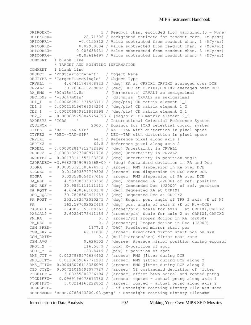
MIPS Instrument Handbook
Introduction to Data Analysis 202
Making Your Own MIPS SED Mosaics
DRIROEXC= 1 / Readout chan. excluded from backgrnd.(0 = None) DRIBKGND= 28.71306 / Background estimate for readout corr. (MJy/sr) DRICORR1= -0.0155812 / Value subtracted from readout chan. 1 (MJy/sr) DRICORR2= 0.02950604 / Value subtracted from readout chan. 2 (MJy/sr) DRICORR3= 0.006658931 / Value subtracted from readout chan. 3 (MJy/sr) DRICORR4= -0.03616497 / Value subtracted from readout chan. 4 (MJy/sr) COMMENT 1 blank line / TARGET AND POINTING INFORMATION COMMENT 1 blank line OBJECT = '2ndStarToTheLeft' / Object Name OBJTYPE = 'TargetFixedSingle' / Object Type CRVAL1 = 4.67411748468823 / [deg] RA at CRPIX1,CRPIX2 averaged over DCE CRVAL2 = 30.7836819259082 / [deg] DEC at CRPIX1,CRPIX2 averaged over DCE RA_HMS = '00h18m41.8s' / [hh:mm:ss.s] CRVAL1 as sexigesimal DEC_DMS = '+30d47m01s' / [dd:mm:ss] CRVAL2 as sexigesimal CD1_1 = 0.000662521671553711 / [deg/pix] CD matrix element 1_1 CD1_2 = 0.000216196769364234 / [deg/pix] CD matrix element 1_2 CD2_1 = 0.000206849911868398 / [deg/pix] CD matrix element 2_1 CD2_2 = -0.000689758045754793 / [deg/pix] CD matrix element 2_2 RADESYS = 'ICRS ' / International Celestial Reference System EQUINOX = 2000. / Equinox for ICRS celestial coord. system CTYPE1 = 'RA---TAN-SIP' / RA---TAN with distortion in pixel space CTYPE2 = 'DEC--TAN-SIP' / DEC--TAN with distortion in pixel space CRPIX1 = 64.5 / Reference pixel along axis 1 CRPIX2 = 64.5 / Reference pixel along axis 2 CRDER1 = 0.000302817912732396 / [deg] Uncertainty in CRVAL1 CRDER2 = 0.000310227340971778 / [deg] Uncertainty in CRVAL2 UNCRTPA = 0.00173141556123278 / [deg] Uncertainty in position angle CSDRADEC= -3.96827849099566E-05 / [deg] Costandard deviation in RA and Dec SIGRA = 0.00995321683674971 / [arcsec] RMS dispersion in RA over DCE SIGDEC = 0.012893579799308 / [arcsec] RMS dispersion in DEC over DCE SIGPA = 0.023538054297016 / [arcsec] RMS dispersion of PA over DCE RA_REF = 4.58708333333336 / [deg] Commanded RA (J2000) of ref. position DEC_REF = 30.9561111111111 / [deg] Commanded Dec (J2000) of ref. position RA_RQST = 4.67438563100378 / [deg] Requested RA at CRPIX1 DEC_RQST= 30.7828569421983 / [deg] Requested Dec at CRPIX2 PA_RQST = 253.183572010275 / [deg] Reqst. pos. angle of TPF Z axis (E of N) PA = 162.597002022419 / [deg] pos. angle of axis 2 (E of N,+=CCW) PXSCAL1 = -2.49861956108361 / [arcsec/pix] Scale for axis 1 at CRPIX1,CRPIX2 PXSCAL2 = 2.60224775411189 / [arcsec/pix] Scale for axis 2 at CRPIX1,CRPIX2 PM_RA = 0. / [arcsec/yr] Proper Motion in RA (J2000) PM_DEC = 0. / [arcsec/yr] Proper Motion in Dec (J2000) CSM_PRED= 1877.5 / [DAC] Predicted mirror start pos CSM_SKY = 69.11006 / [arcsec] Predicted mirror start pos on sky CSM_RATE= 0. / [milli-arcsec/sec] Mirror scan rate CSM_AVG = 0.626502 / [degree] Average mirror position during exposur SPOT_X = 116.5679 / [pix] X-position of spot SPOT_Y = 123.8449 / [pix] Y-position of spot RMS_JIT = 0.0127988574634452 / [arcsec] RMS jitter during DCE RMS_JITY= 0.0110659867771283 / [arcsec] RMS jitter during DCE along Y RMS_JITZ= 0.00643076115386099 / [arcsec] RMS jitter during DCE along Z CSD_JTYZ= 0.00721015496077727 / [arcsec] YZ costandard deviation of jitter PTGDIFF = 3.08355809766194 / [arcsec] offset btwn actual and rqsted pntng PTGDIFFX= 0.0969196073613785 / [arcsec] rqsted - actual pntng along axis 1 PTGDIFFY= 3.08214166222852 / [arcsec] rqsted - actual pntng along axis 2 USEDBPHF= T / T if Boresight Pointing History File was used BPHFNAME= 'BPHF.0788443200.03.pntg' / Boresight Pointing History Filename
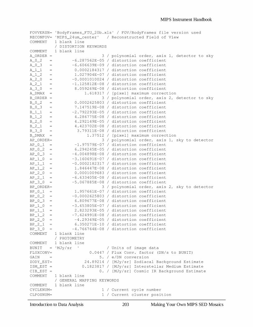
MIPS Instrument Handbook
Introduction to Data Analysis 203
Making Your Own MIPS SED Mosaics
FOVVERSN= 'BodyFrames_FTU_20b.xls' / FOV/BodyFrames file version used RECONFOV= 'MIPS_24um_center' / Reconstructed Field of View COMMENT 1 blank line / DISTORTION KEYWORDS COMMENT 1 blank line A_ORDER = 3 / polynomial order, axis 1, detector to sky A_0_2 = -6.287562E-05 / distortion coefficient A_0_3 = -6.606639E-09 / distortion coefficient A_1_1 = 0.0002184317 / distortion coefficient A_1_2 = 1.027904E-07 / distortion coefficient A_2_0 = -0.0001010024 / distortion coefficient A_2_1 = -1.125812E-08 / distortion coefficient A_3_0 = 8.059269E-08 / distortion coefficient A_DMAX = 1.618317 / [pixel] maximum correction B_ORDER = 3 / polynomial order, axis 2, detector to sky B_0_2 = 0.0002625803 / distortion coefficient B_0_3 = 7.147519E-08 / distortion coefficient B_1_1 = -2.792293E-05 / distortion coefficient B_1_2 = 4.286775E-08 / distortion coefficient B_2_0 = 4.292149E-05 / distortion coefficient B_2_1 = 4.423702E-08 / distortion coefficient B_3_0 = 3.79311E-08 / distortion coefficient B_DMAX = 1.37512 / [pixel] maximum correction AP_ORDER= 3 / polynomial order, axis 1, sky to detector AP_0_1 = -1.97579E-07 / distortion coefficient AP_0_2 = 6.294245E-05 / distortion coefficient AP_0_3 = -4.004898E-08 / distortion coefficient AP_1_0 = -3.160691E-07 / distortion coefficient AP_1_1 = -0.0002182317 / distortion coefficient AP_1_2 = 1.846447E-08 / distortion coefficient AP_2_0 = 0.0001009683 / distortion coefficient AP_2_1 = -6.633405E-08 / distortion coefficient AP_3_0 = -5.067885E-08 / distortion coefficient BP_ORDER= 3 / polynomial order, axis 2, sky to detector BP_0_1 = 1.957661E-07 / distortion coefficient BP_0_2 = -0.0002625803 / distortion coefficient BP_0_3 = 6.809677E-08 / distortion coefficient BP_1_0 = -3.653805E-07 / distortion coefficient BP_1_1 = 2.823293E-05 / distortion coefficient BP_1_2 = -7.624991E-08 / distortion coefficient BP_2_0 = -4.29349E-05 / distortion coefficient BP_2_1 = 6.350271E-10 / distortion coefficient BP_3_0 = -4.766764E-08 / distortion coefficient COMMENT 1 blank line / PHOTOMETRY COMMENT 1 blank line BUNIT = 'MJy/sr ' / Units of image data FLUXCONV= 0.0447 / Flux Conv. factor (DN/s to BUNIT) GAIN = 5. / e/DN conversion ZODY_EST= 24.89214 / [MJy/sr] Zodiacal Background Estimate ISM_EST = 0.1823817 / [MJy/sr] Interstellar Medium Estimate CIB_EST = 0. / [MJy/sr] Cosmic IR Background Estimate COMMENT 1 blank line / GENERAL MAPPING KEYWORDS COMMENT 1 blank line CYCLENUM= 1 / Current cycle number CLPOSNUM= 1 / Current cluster position

MIPS Instrument Handbook
Introduction to Data Analysis 204
Making Your Own MIPS SED Mosaics
COMMENT 1 blank line / MIPS PHOTOMETRY-SUPER RESOLUTION COMMENT 1 blank line SELEC24 = T / MIPS-24 selected LARGE24 = F / MIPS-24 Field Size; T=large, F=small NCYCL24 = 1 / Number of MIPS-24 photometry cycles SELEC70 = T / MIPS-70 selected LARGE70 = F / MIPS-70 Field Size; T=large, F=small FINESCAL= F / Image scale (T= fine, F=default) NCYCL70 = 2 / Number of MIPS-70 photometry cycles SELEC160= F / MIPS-160 selected COMMENT 1 blank line / INSTRUMENT TELEMETRY DATA COMMENT 1 blank line CE_SIDE = 1 / Common Electronics Side (1=A,2=B) GRPARVTC= 7.884455E+08 / [Sec] Coarse Spacecraft Group Time GRPARVTF= 0.687874 / [Sec] Fine Spacecraft Group Time CRSESYNC= 788445529 / [Sec] Mirror Sync Pulse Coarse Time FINESYNC= 41070. / [1/65535 Sec] Mirror Sync Pulse Fine Time CSM_MOD = 0 / CSMM Mode: 0=Chop,1=Ramp DCE_FRMS= 84 / [Fr/DCE] Ge Frames per DCE Command FRMFLYBK= 4 / [Frames] CSMM Flyback Duration CSM_SLP = 511. / [DAC/s] CSMM Ramp Slope Command DCE_CALC= 6 / DCEs per Calibration Cycle Command ACREJCNT= 0 / Command Reject Counter AIRSPCNT= 0 / Invalid Response Count ALIMVCNT= 0 / Limit Violation Counter AFIFOBAD= 1 / Science Data FIFO Bad Half Full Interrupts ASDMGRFA= 0 / SDM Groups Not Accepted By CDH ALSTERLD= 3732 / Last Error Id ALSTERPM= 1 / Last Error Parameter ATOTALER= 6 / Total Errors Posted Count CSM_POS = 29944. / [DAC] CSMM Position Output CSM_POSF= 23760.3333333333 / [DAC] CSMM Fine Position DAC CSM_POSC= 16732.6666666667 / [DAC] CSMM Coarse Position DAC ANCSMCUR= -539.536576666667 / [uAmps] ANCSMGN = -14.9433215555556 / CSMM Gain Adjustment DAC CSM_OFFS= 2367.14527777778 / [arcsec] CSMM Position Offset DAC Output ANCSMPS1= 2007. / [DAC] CSMM Scanpos1 Command ANCSMPS2= 2007. / [DAC] CSMM Scanpos2 Command ANCSMRP1= 2307. / [DAC] CSMM Relpos1 Command ANCSMRP2= 3602. / [DAC] CSMM Relpos2 Command ANCSMSTP= -259. / [DAC] CSMM Scanoffset Command CMD_DCES= 13 / Number of DCEs in Exposure CSM_OOLC= 0 / CSMM Out Of Limits Count SC_SYNCC= 40484 / Total HTG CSMM to SC Synch Pulse Count GROUPCNT= 4 / MIPS Group Count Per DCE GROUPIDX= 74 / MIPS Exp. Manager Index for Next SDM Group ANIMCYFC= 84 / Frames per Image Cycle Commanded ANHTGEFC= 429 / HTG Frames In Exposure Counter IMGCYCLC= 20878 / Total Image Cycles Since HTG Ready EXPIMGCY= 5 / Image Cycles in Exposure Counter ANCALCYC= 4 / DCEs completed in Calibration Cycle D24FRAME= 61994 / Total D24 Frame Count D24EXPDC= 4 / D24 DCEs in Exposure Counter CMD_T_24= 5.15 / [Deg_K] AD24TMPA= 5.156204 / [Deg_K]

MIPS Instrument Handbook
Introduction to Data Analysis 205
Making Your Own MIPS SED Mosaics
AD24TMPB= 5.13661 / [Deg_K] ACSMMTMP= 1.267753 / [Deg_K] ACEBOXTM= 13.00376 / [Deg_C] AD24STMI= 0. / [uAmps] AD24HTRI= 104.8543 / [uAmps] AVDSUBV = 3.492988 / [Volts] VD Sub Voltage APROFF1V= 5.907892 / [Volts] APROFF2V= 5.904685 / [Volts] APROFF3V= 5.903617 / [Volts] APROFF4V= 5.903403 / [Volts] AD24ANLI= 1181.821 / [uAmps] ABASTMCR= 788427678 / Coarse Component of CE Base Time ABASTMFN= 15353 / Fine Component of CE Base Time AFSWMJRV= 3 / CE Flight Software Major Version Number AFSWMINV= 2 / CE Flight Software Minor Version Number AD24PWEN= 1 / Det 24u Power Enable Commanded State AD24SITM= 0 / Det 24u Temperature Sensor Status AD24PWRS= 1 / Det 24u Power Enable Status AD24TMSE= 1 / Det 24u Temperature Sensor Comanded State AD24STMC= 0 / Det 24u Stimulator Enable Commanded State A24HTDAC= 244 / D24 Heater DAC Load Value A24HTCMD= 1 / MIPS D24 Heater Enable Commanded State AD24ANLS= 0 / MIPS D24 Anneal Status A24HTMEN= 1 / D24 Heater Monitor Enable Status HSPLSTMF= 60546 / MIPS Scan Mirror Pulse Timestamp Fine SC_AT_Q1= 0.7792743 / ATDT_SC_QUATERNION_Q1 SC_AT_Q2= -0.1274316 / ATDT_SC_QUATERNION_Q2 SC_AT_Q3= 0.2363692 / ATDT_SC_QUATERNION_Q3 SC_AT_Q4= 0.5662352 / ATDT_SC_QUATERNION_Q4 SC_R8_X = 0.09427691 / [asec/s] SC_R8_Y = -0.03779747 / [asec/s] SC_R8_Z = 0.02729783 / [asec/s] COMMENT 1 blank line / DATA FLOW KEYWORDS COMMENT 1 blank line DATE = '2009-12-08T04:25:11' / [YYYY-MM-DDThh:mm:ss UTC] file creation date ORIGIN0 = 'JPL_FOS ' / Site where raw-FITS file was written CREATOR0= 'JPL_FOS SIS' / SW system that created raw-FITS file SIS_SVER= 'J5.3 ' / SIS SW VERsion of CREATOR0 AORKEY = 11254784 / AOR or IER key. Astro. Obs Req/Instr Eng Req DS_IDENT= 'ads/sa.spitzer#0011254784' / Data Set Identification for ADS/journals EXPID = 3 / Exposure ID (0-9999) DCENUM = 4 / DCE number (0-9999) TLMGRPS = 9 / Number of expected telemetry groups FILE_VER= 1 / Version of the raw file made by SIS RAWDATE = '2004-12-25T13:10:25' / SIS file creation date RAWFILE = 'MIPS.1.0011254784.0003.0004.01.mipl.fits' / Raw data file name CPT_VER = '3.0.98 ' / Channel Param Table FOS versioN EXPDFLAG= F / (T/F) expedited DCE MISS_LCT= 0 / Total Missed Line Cnt in this FITS MANCPKT = F / T if this FITS is Missing Ancillary Data MISSDATA= F / T if this FITS is Missing Image Data PAONUM = 987 / PAO Number CAMPAIGN= 'MIPS007100' / Campaign DCEID = 25153227 / Data-Collection-Event ID DCEINSID= 5382760 / DCE Instance ID DPID = 290022187 / Data Product Instance ID
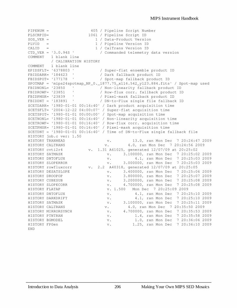
MIPS Instrument Handbook
Introduction to Data Analysis 206
Making Your Own MIPS SED Mosaics
PIPENUM = 405 / Pipeline Script Number PLSCRPID= 1061 / Pipeline Script ID SOS_VER = 1 / Data-Product Version PLVID = 1 / Pipeline Version ID CALID = 1 / CalTrans Version ID CTD_VER = '3.0.94S ' / Commanded telemetry data version COMMENT 1 blank line / CALIBRATION HISTORY COMMENT 1 blank line EPIDSFLT= '6378803 ' / Super-flat ensemble product ID FBIDDARK= '184623 ' / Dark fallback product ID FBIDSPOT= '177178 ' / Spot-map fallback product ID SPOTMAP = 'mips24spotmap_NP_0._1877.75_x116.542_y123.884.fits' / Spot-map used FBIDNONL= '23850 ' / Non-linearity fallback product ID FBIDROWF= '23851 ' / Row-flux corr. fallback product ID FBIDPMSK= '23839 ' / Pixel-mask fallback product ID FBIDDNT = '183891 ' / DN-to-Flux single file fallback ID SCETDARK= '1980-01-01 00:16:40' / Dark product acquisition time SCETSFLT= '2004-12-22 04:00:07' / Super-flat acquisition time SCETSPOT= '1980-01-01 00:00:00' / Spot-map acquisition time SCETNONL= '1980-01-01 00:16:40' / Non-linearity acquisition time SCETROWF= '1980-01-01 00:16:40' / Row-flux corr. acquisition time SCETPMSK= '1980-01-01 00:16:40' / Pixel-mask acquisition time SCETDNT = '1980-01-01 00:16:40' / Time of DN-to-Flux single fallback file HISTORY job.c ver: 1.50 HISTORY TRANHEAD v. 13.0, ran Mon Dec 7 20:24:47 2009 HISTORY CALTRANS v. 4.0, ran Mon Dec 7 20:24:56 2009 HISTORY cvti2r4 v. 1.31 A61025, generated 12/07/09 at 20:25:02 HISTORY SATMASK v. 3.100000, ran Mon Dec 7 20:25:02 2009 HISTORY DNTOFLUX v. 4.1, ran Mon Dec 7 20:25:03 2009 HISTORY SLOPERROR v. 3.000000, ran Mon Dec 7 20:25:03 2009 HISTORY rowfluxcorr v. 2.2 A40318, generated 12/07/09 at 20:25:05 HISTORY DESATSLOPE v. 3.400000, ran Mon Dec 7 20:25:06 2009 HISTORY DROOPOP v. 3.800000, ran Mon Dec 7 20:25:07 2009 HISTORY CUBESUB v. 3.200000, ran Mon Dec 7 20:25:08 2009 HISTORY SLOPECORR v. 4.700000, ran Mon Dec 7 20:25:08 2009 HISTORY FLATAP v. 1.500 Mon Dec 7 20:25:09 2009 HISTORY DNTOFLUX v. 4.1, ran Mon Dec 7 20:25:10 2009 HISTORY DARKDRIFT v. 4.1, ran Mon Dec 7 20:25:10 2009 HISTORY SATMASK v. 3.100000, ran Mon Dec 7 20:25:11 2009 HISTORY CALTRANS v. 4.0, ran Mon Dec 7 20:35:50 2009 HISTORY MIRRORSYNCH v. 4.700000, ran Mon Dec 7 20:35:53 2009 HISTORY PTNTRAN v. 1.4, ran Mon Dec 7 20:35:58 2009 HISTORY BGMODEL v. 1.0, ran Mon Dec 7 20:36:06 2009 HISTORY FPGen v. 1.25, ran Mon Dec 7 20:36:10 2009 END

MIPS Instrument Handbook
Introduction to Data Analysis 207
Making Your Own MIPS SED Mosaics
Appendix E. List of FiguresFIGURE 2.1: SCHEMATIC DIAGRAM OF THE MIPS OPTICAL TRAIN, DETECTORS ......................................10FIGURE 2.2: (TOP) A 24 MICRON PSF WITH THE DISPLAY PARAMETERS STRETCHED TO SHOW THE
CENTRAL PEAK AND FIRST RING ONLY. (BOTTOM). THE SAME 24 MICRON PSF WITH THE DISPLAY PARAMETERS STRETCHED TO SHOW THE FULL PSF IN THE SAME 5 X 5 ARCMINUTE FIELD OF VIEW. 13
FIGURE 2.3: PRE-LAUNCH RESPONSE OF THE 24 µM BAND INCLUDING DETECTOR AND FILTER SPECTRAL RESPONSE. ................................................................................................................................15
FIGURE 2.4: PRE-LAUNCH RESPONSE OF THE 70 µM BAND INCLUDING DETECTOR AND FILTER SPECTRAL RESPONSE. ................................................................................................................................15
FIGURE 2.5: PRE-LAUNCH RESPONSE OF THE 160 µM BAND INCLUDING DETECTOR AND FILTER SPECTRAL RESPONSE.. ...............................................................................................................................16
FIGURE 2.6: PRE-LAUNCH SED SPECTRAL RESPONSE INCLUDING DETECTOR, FILTERS, AND GRATING EFFICIENCY. .............................................................................................................................16
FIGURE 2.7: 70 µM ARRAY 4X32 SUBMODULE. ....................................................................................19FIGURE 2.8: ASSEMBLED 70 µM FOCAL PLANE. ...................................................................................20FIGURE 2.9: 1X5 SUBMODULE OF THE 160 µM ARRAY SHOWING DISCRETE PIXEL ELEMENTS, INTEGRATING
CAVITIES, AND READOUT. ..........................................................................................................20FIGURE 2.10: STRESSING RIG FOR THE 160 µM ARRAY VIEWED EDGE-ON. ..............................................21FIGURE 2.11: FULLY-ASSEMBLED 160 µM FOCAL PLANE ARRAY SHOWING 4 STRESSING RIGS, EACH
CONTAINING TWO 1X5 SUBMODULES, AND SHOWING THE PHOTON CONCENTRATOR CONES. ..........21FIGURE 2.12: SCHEMATIC RESPONSE CHARACTERISTICS OF A BULK PHOTOCONDUCTOR. . .....................25FIGURE 2.13: MEASURED RESPONSE OF A PIXEL OF THE MIPS 70 µM ARRAY TO A SUDDEN INCREASE IN
ILLUMINATION FROM A DARK BACKGROUND. ............................................................................26FIGURE 2.14: ELECTRONIC SCHEMATIC FOR MIPS/IRS COMBINED ELECTRONICS PACKAGE. ..................28FIGURE 2.15: MIPS SOFTWARE BLOCK DIAGRAM. ...............................................................................30FIGURE 2.16: SENSITIVITY IN SCAN MAP MODE AT 24 µM. ...................................................................35FIGURE 2.17: SENSITIVITY FOR PHOTOMETRY AT 24 µM, COMPACT SOURCE (I.E., ONE THAT CAN ALWAYS
BE KEPT ON THE ARRAY DURING THE MEASUREMENT). ................................................................36FIGURE 3.1: PHOTOMETRY/SUPER RESOLUTION FOR COMPACT SOURCES WITH THE 24 µM ARRAY. . ......42FIGURE 3.2: OBSERVING A LARGE-DIAMETER SOURCE AT 24 µM. . .......................................................44FIGURE 3.3: PHOTOMETRY OF A COMPACT SOURCE WITH THE 70 µM ARRAY. . ......................................46FIGURE 3.4: SIMULATED SOURCE DETECTIONS ON THE ARRAY DURING THE COMPACT SOURCE
PHOTOMETRY AOT IN FIGURE 3.3. ...........................................................................................47FIGURE 3.5: PHOTOMETRY OF A LARGE SOURCE AT 70 µM. . ................................................................49FIGURE 3.6: SIMULATED SOURCE DETECTIONS ON THE ARRAY DURING THE LARGE SOURCE PHOTOMETRY
AOT SHOWN IN FIGURE 3.5. . ....................................................................................................50FIGURE 3.7: POSITIONS OF THE SOURCE RELATIVE TO THE 160 µM ARRAY DURING THE COMPACT SOURCE
PHOTOMETRY AOT. . ...............................................................................................................51FIGURE 3.8: SIMULATED VISUALIZATION OF INDIVIDUAL FRAMES IN THE FIRST CYCLE OF THE 160 µM
SMALL SOURCE PHOTOMETRY AOT SHOWN IN FIGURE 3.7. .........................................................52FIGURE 3.9: PHOTOMETRY OF A 4´X5.3 ́REGION AT 160 µM. . ..............................................................53FIGURE 3.10: THE DATA ACQUISITION SEQUENCE FOR THE 160 µM LARGE-SOURCE OPTION. . ................54FIGURE 3.11: ASTEROID HARMONIA OBSERVED USING THE 160 µM ENHANCED MODE DURING MC42
(JULY 2007).. ............................................................................................................................55FIGURE 3.12: A COMPARISON OF PHOTOMETRIC OBSERVATIONS OF 3C371 AT 160 µM USING THE
ENHANCED MODE (LEFT) AND THE ''DEFAULT'' SMALL-FIELD MODE (RIGHT), OBTAINED DURING MC41 (2007 JUNE). .................................................................................................................56
FIGURE 3.13: SOURCE POSITIONS ON THE 70 µM ARRAY DURING THE SUPER RESOLUTION AOT FOR A COMPACT SOURCE. ..................................................................................................................57

MIPS Instrument Handbook
Introduction to Data Analysis 208
Making Your Own MIPS SED Mosaics
FIGURE 3.14: SOURCE DETECTIONS ON THE ARRAY DURING THE 70 µM COMPACT SOURCE SUPER RESOLUTION PHOTOMETRY AOT SHOWN IN FIGURE 3.13.. ...........................................................58
FIGURE 3.15: STRATEGY FOR OBTAINING SUPER RESOLUTION OBSERVATIONS OVER A FIELD OF 2.5´X2.5 .́ ................................................................................................................................................59
FIGURE 3.16: SCHEMATIC REPRESENTATION OF SYNCHRONIZATION OF SCAN MIRROR MOTIONS, TELESCOPE SCAN, AND STIMULATOR FLASHES. ...........................................................................63
FIGURE 3.17: OPERATION OF 24 AND 70 µM ARRAYS DURING SCAN MAPPING. . ....................................63FIGURE 3.18: MIPS OPERATION AT 160 µM IN SCAN MAP MODE. . ........................................................65FIGURE 3.19: SCHEMATIC REPRESENTATION OF SED MODE; SEE TEXT. . ..............................................68FIGURE 4.1: MIPS FLAT FIELD POSITIONS INDICATED ON A DIRBE 140 MICRON ALL-SKY MAP. .............80FIGURE 4.2: AN SED SPECTRUM OF THE BRIGHT PLANETARY NEBULA NGC 6543. ...............................81FIGURE 4.3: THE RATIO OF THE MEASURED-TO-PREDICTED FLUX DENSITIES FOR SED CALIBRATION STARS
AT (A) 60 µM, (B) 71.4 µM, AND (C) 80 µM, AS A FUNCTION OF THE PREDICTED 71.4µM FLUX DENSITY. . ...............................................................................................................................................87
FIGURE 4.4: COMPARISONS OF SED FLUXES (AS A SOLID LINE) WITH IRAS 60 AND 100 µM FLUXES FOR THE GALAXY NGC 4418. ...........................................................................................................88
FIGURE 4.5: EXAMPLE SOURCE FROM 24 MICRON EXTRAGALACTIC FIRST-LOOK SURVEY (XFLS) FOR EXAMPLE APERTURE CORRECTIONS. ...........................................................................................94
FIGURE 4.6: EXAMPLE APERTURE CORRECTIONS FOR 24 MICRON DATA (SEE TEXT). THE FWHM IS 5.9 ARCSEC. ...................................................................................................................................97
FIGURE 5.1: MIPS 24 MICRON PIPELINE. ........................................................................................... 106FIGURE 5.2: AUTOMATED MIPS-24 PIPELINE PRODUCTS : RAW DATA (DCE). . ................................... 107FIGURE 5.3: AUTOMATED MIPS-24 PIPELINE PRODUCTS: SINGLE BCD. . ........................................... 108FIGURE 5.4: AUTOMATICALLY-PRODUCED MOSAIC COMBINING MULTIPLE BCDS FROM A PHOTOMETRY
OBSERVATION. ........................................................................................................................ 108FIGURE 5.5: AUTOMATICALLY-PRODUCED MOSAIC COMBINING MULTIPLE BCDS FROM A SCAN MAP
OBSERVATION. ........................................................................................................................ 109FIGURE 5.6: MIPS GE (70 AND 160 µM) SCIENCE PIPELINE. ................................................................ 111FIGURE 5.7: THE MIPS POST-BCD PIPELINE. . .................................................................................. 113FIGURE 6.1: ILLUSTRATION OF TWO TYPICAL BCD IMAGES TAKEN RESPECTIVELY AT THE TWO DITHER
POSITIONS OF THE SED MODE. . ............................................................................................... 125FIGURE 6.2: AN EXAMPLE OF AN OVERALL SMOOTH (SPOT-FREE) GAINFLAT IMAGE. ........................... 127FIGURE 6.3: EXAMPLE SPOTMAP IMAGES.. ........................................................................................ 128FIGURE 6.4: A SMALL FIELD PHOTOMETRY EXAMPLE, DEMONSTRATING THE S18.12 EBCD FLAT FIELDING
IMPROVEMENTS.. .................................................................................................................... 130FIGURE 6.5: AN EXAMPLE OF THE SIGNIFICANT IMPROVEMENT OF 24 MICRON DATA TAKEN IN PARALLEL
MODE.. ................................................................................................................................... 130FIGURE 6.6: PLOT OF THE POST-BCD EXTRACTED SPECTRUM (SQUARES) FROM AN OBSERVATION OF THE
STAR. ..................................................................................................................................... 131FIGURE 6.7: BAD PIXEL MASK FOR 24 MICRONS. ............................................................................... 135FIGURE 6.8: BAD PIXEL MASK (PMASK) FOR MIPS-70 DATA. ............................................................ 135FIGURE 6.9: BAD PIXEL MASK (PMASK) FOR MIPS-160 DATA. . ......................................................... 136FIGURE 7.1: SAMPLE MIPS-24 PHOTOMETRY MOSAIC PRODUCT (SEVERAL COMBINED BCDS) FROM
BEFORE THE READ-2 CORRECTION. ........................................................................................... 140FIGURE 7.2: SAMPLE SUBSECTION OF MIPS-24 SCAN MAP. . .............................................................. 141FIGURE 7.3: TWO MIPS-24 FLAT FIELDS AT TWO DIFFERENT SCAN MIRROR POSITIONS. ...................... 142FIGURE 7.4: PICK-OFF MIRROR SPOTS BEFORE (LEFT, CIRCLED IN RED), AND AFTER (RIGHT) USING SCAN
MIRROR POSITION DEPENDENT FLATS ON A CALIBRATION STAR OBSERVATION. ........................... 143FIGURE 7.5: MAP OF THE SPOT LOCATIONS BASED ON 24 MICRON OBSERVATIONS. .............................. 143FIGURE 7.6: RESULTS OF DIVIDING MISMATCHED POSITION-DEPENDENT FLAT FROM THE DATA - ZOOM IN
ON JUST ONE SPOT. .................................................................................................................. 143

MIPS Instrument Handbook
Introduction to Data Analysis 209
Making Your Own MIPS SED Mosaics
FIGURE 7.7: EXAMPLE OF ''JAILBAR'' EFFECT FROM A SATURATED POINT SOURCE ................................ 145FIGURE 7.8: EXAMPLE OF SHORT-LIVED BRIGHT LATENTS. ................................................................ 145FIGURE 7.9: INITIAL BCD AFFECTED BY BRIGHT SOURCES ................................................................. 146FIGURE 7.10: BCD AFTER ADDITIVE JAILBAR CORRECTION. ............................................................... 147FIGURE 7.11: BCD AFTER ''SELF-CALIBRATION'' TO CORRECT DARK LATENTS. .................................... 147FIGURE 7.12: EXAMPLE OF DARK LATENTS ALL BY THEMSELVES. . .................................................... 148FIGURE 7.13: EXAMPLE OF LONG-LIVED BRIGHT LATENTS WITH NEWER DARK LATENTS. ..................... 149FIGURE 7.14: BCDS FROM AORS LATER IN THE CAMPAIGN WHERE THE DATA IN FIGURE 7.13 WERE
OBTAINED. ............................................................................................................................ 149FIGURE 7.15: EVIDENCE OF SLOW RESPONSE DRIFT IN TWO ELAIS-N1 DEEP 24 MICRON FIELDS. ......... 150FIGURE 7.16: VERY RARE GLINT - FAKE ~12 JY SOURCE SEEN ~1.5 DEGREES FROM ~1500 JY SOURCE. . 151FIGURE 7.17: EXAMPLE OF SINGLE FRAME WITH ZERO-LEVEL OFFSET. NO BACKGROUND MATCHING WAS
PERFORMED IN CREATING THIS MOSAIC. ................................................................................... 152FIGURE 7.18: BEWARE OF ASTEROIDS! MOST OF THE POINT SOURCES IN THIS FRAME ARE ASTEROIDS. 153FIGURE 7.19: EXAMPLES OF SEVERAL OF THE MOST COMMON MIPS-70 ARTIFACTS. ........................... 154FIGURE 7.20: DEFAULT MOSAIC FROM 4 AORS OF UNFILTERED MIPS-70 BCDS. .............................. 155FIGURE 7.21: AUTOMATICALLY-PRODUCED MOSAICS OF NGC 300. . ................................................ 156FIGURE 7.22: EFFECTS OF EXTRAPOLATED STIM CALIBRATION. ........................................................ 157FIGURE 7.23: 160 MICRON IMAGE OF AN ASTEROID; COMPARE TO NEXT 2 FIGURES. . .......................... 159FIGURE 7.24: 160 MICRON IMAGE OF A STAR; COMPARE TO PREVIOUS AND NEXT FIGURE. .................... 159FIGURE 7.25: SCALED ASTEROID - THIS IS THE BRIGHTNESS OF THE PHOTOSPHERE COMPARED TO THE
LEAK. ..................................................................................................................................... 159FIGURE 7.26: ANOTHER VIEW OF THE SPECTRAL LEAK. ..................................................................... 160FIGURE 7.27: EXAMPLES OF 70 MICRON FINE SCALE REPROCESSING DISCUSSED IN TEXT. ..................... 161FIGURE 7.28: APPLYING THE SAME TECHNIQUE TO A SMALL RASTER MAP OBSERVATION. .................... 162FIGURE 8.1: EXAMPLE MOSAIC BEFORE, WITH LONG-TERM BRIGHT LATENTS AND WEAK JAILBARS, AND
AFTER SELF-CALIBRATION, WHERE THOSE EFFECTS ARE WELL-CORRECTED. . ............................ 164FIGURE 8.2: EXAMPLE MOSAIC BEFORE, WITH LONG-TERM DARK LATENTS, AND AFTER SELF
CALIBRATION OF PHOTOMETRY DATA USING NON-PRIME DATA. ................................................. 164FIGURE 8.3: ANOTHER EXAMPLE OF SELF-CALIBRATION REMOVING DARK LATENTS, THIS TIME IN A
LARGE SCAN MAP. LEFT IS BEFORE, RIGHT IS AFTER. ................................................................. 165FIGURE 8.4: NGC 300 IN 24 MICRONS, ROTATED TO HAVE NORTH UP. THE LEFT IMAGE IS THE STANDARD
POST-BCD MOSAIC. ................................................................................................................ 166FIGURE 8.5: DEFAULT MOSAIC FROM FILTERED MIPS-70 BCDS, CONSTRUCTED FROM 4 AORS. .......... 168FIGURE 8.6: A FLOWCHART DESCRIBING POSSIBLE PATHWAYS FOR ANALYSIS OF SCAN MAP POST-BCD GE
DATA PROCESSING. . ............................................................................................................... 169FIGURE 8.7: STEP 1: MOSAIC OF INITIAL DEFAULT 70 MICRON SCAN BCDS (1 AOR) FROM THE
EXTRAGALACTIC FIRST LOOK SURVEY. . ................................................................................. 171FIGURE 8.8: STEP 2: MOSAIC OF TIME-FILTERED 70 MICRON SCAN BCDS FOR 1 AOR. ........................ 172FIGURE 8.9: STEP 3: MOSAIC OF COLUMN-FILTERED 70 MICRON SCAN BCDS FOR 1 AOR. .................... 172FIGURE 8.10: STEP 4: MOSAIC OF 4 AORS PROCESSED WITH BOTH COLUMN AND TIME FILTER. ............. 173FIGURE 8.11: MOSAIC OF MIPS-160 DEFAULT SCAN BCDS FROM THE EXTRAGALACTIC FLS. .............. 174FIGURE 8.12: MOSAIC OF MIPS-160 FILTERED SCAN BCDS (*FBCD FILES). ........................................ 174FIGURE 8.13: MOSAIC OF 70 MICRON BCDS FROM NGC 300. ............................................................. 176FIGURE 8.14: EXAMPLE OF OFFLINE PROCESSING USING THE GERT USING A SERIES OF IMAGES OF NGC
7331. . ................................................................................................................................... 176FIGURE 8.15: MOSAIC OF UNFILTERED AND FILTERED. ...................................................................... 177FIGURE 8.16: SCAN MAP OF THE MOLECULAR CLOUD L1228 AT 160 MICRONS FROM THE GALACTIC FIRST
LOOK SURVEY (2 DEGREES LONG). . ........................................................................................ 178FIGURE 8.17: AS ABOVE, BUT USING THE FILTERED BCDS;. ............................................................... 178

MIPS Instrument Handbook
Introduction to Data Analysis 210
Making Your Own MIPS SED Mosaics
FIGURE 8.18 : THE INTEGRATED FLUX OF THE L1228 MOSAIC ON THE CROSS-SCAN DIRECTION ALONG THE SCANNING DIRECTION FOR THE UNFILTERED AND FILTERED. .............................................. 178

MIPS Instrument Handbook
Introduction to Data Analysis 211
Making Your Own MIPS SED Mosaics
Appendix F. List of TablesTABLE 2.1: MIPS PRINCIPAL OPTICAL PARAMETERS. ...........................................................................11TABLE 2.2: MIPS SPECTRAL RESPONSE SUMMARY. .............................................................................14TABLE 2.3: OPTICAL DISTORTION IN MIPS. ........................................................................................17TABLE 2.4: MIPS SI:AS BIB ARRAY PERFORMANCE CHARACTERISTICS. ...............................................22TABLE 2.5: MIPS GE:GA ARRAY PERFORMANCE CHARACTERISTICS. ....................................................23TABLE 2.6: CONVERSION FROM POINT SOURCE SENSITIVITY TO EXTENDED SOURCE SENSITIVITY.* ........36TABLE 2.7: MIPS SATURATION LEVELS. .............................................................................................37TABLE 2.8: MIPS 24 µM POINT-SOURCE SATURATION LEVEL EXPRESSIONS INCLUDING SKY. .................37TABLE 2.9: MIPS 24 µM SOFT SATURATION LEVELS. ...........................................................................39TABLE 3.1: SOURCE POSITIONS FOR 24 µM COMPACT SOURCE PHOTOMETRY ........................................42TABLE 3.2: SOURCE POSITIONS FOR 24 µM LARGE SOURCE PHOTOMETRY .............................................44TABLE 3.3: SOURCE POSITIONS FOR 70 µM DEFAULT PIXEL SCALE COMPACT SOURCE PHOTOMETRY. ......47TABLE 3.4: MIPS PHOTOMETRY AND SUPER-RESOLUTION SUMMARY. ................................................61TABLE 3.5: TOTAL SINGLE-PASS MIPS SCAN MAP INTEGRATION TIME PER PIXEL AND OVERSCAN TIME. .66TABLE 3.6: APPROXIMATE OVERHEAD FACTORS FOR MIPS PHOTOMETRY/SUPER-RESOLUTION. .............69TABLE 4.1: A REPRESENTATIVE SAMPLE OF CALIBRATORS USED. .......................................................73TABLE 4.2: FLUX DENSITIES (JY) OF PRIMARY MIPS CALIBRATORS AT 10.6 µM; RMS ERROR OF 2% IN
FINAL ADOPTED VALUE. ............................................................................................................76TABLE 4.3: COLUMN-WISE CORRECTION FACTORS TO IC. ...................................................................82TABLE 4.4: MEAN SPECTRAL RESPONSE FUNCTION. ...........................................................................83TABLE 4.5: APERTURE CORRECTIONS. ...............................................................................................85TABLE 4.6: TIMELINE OF MIPS/SED IPP FILE UPDATES. .....................................................................89TABLE 4.7: ESTIMATED POINTING OFFSETS. .......................................................................................89TABLE 4.8: ERROR BUDGET FOR FLUX CALIBRATION OF EXTENDED SOURCES. ....................................90TABLE 4.9: SIZES OF MIPS PIXELS FOR MIPS BCD AND POST-BCD PRODUCTS. ....................................91TABLE 4.10: CONVERSION FROM INSTRUMENTAL UNITS TO MJY/SR. ....................................................91TABLE 4.11: CHANGES IN CONVERSION FACTOR WITH PIPELINE. .........................................................92TABLE 4.12: MAGNITUDE ZERO POINTS. .............................................................................................92TABLE 4.13: 24 MICRON APERTURE CORRECTIONS FOR 10,000 K BLACKBODY. .....................................94TABLE 4.14: APERTURE CORRECTIONS FOR 70 MICRONS. .....................................................................95TABLE 4.15: APERTURE CORRECTIONS FOR 160 MICRONS. ...................................................................95TABLE 4.16: NOMINAL COLOR CORRECTIONS VS. BLACKBODY SOURCE TEMPERATURE. ........................98TABLE 4.17: NOMINAL COLOR CORRECTIONS FOR POWER LAWS. .........................................................98TABLE 6.1: COMPLETE LIST OF FILE TYPES FOR MIPS-24. .................................................................. 119TABLE 6.2: COMPLETE LIST OF FILE TYPES FOR MIPS-70 AND MIPS-160. .......................................... 122TABLE 6.3: PRIME AND NON-PRIME DATA. ........................................................................................ 124TABLE 6.4: SOME IMPORTANT POST-BCD FILES FOR MIPS/SED. ...................................................... 132TABLE 6.5: BAD PIXELS IN 24 MICRON ARRAY. ................................................................................. 134TABLE 6.6: BCD BIT MASK DEFINITIONS FOR 24 MICRONS FOUND IN BBMSK.FITS OR EBMSK.FITS FILES.
.............................................................................................................................................. 136TABLE 6.7: BIT MASK DEFINITIONS FOR GE DATA. ............................................................................ 137TABLE A.1: ACRONYMS USED IN THIS MANUAL. ............................................................................... 181

MIPS Instrument Handbook
Acknowledgements 212
Acknowledgements
Appendix G. Acknowledgements The Multiband Imaging Photometer for Spitzer (MIPS) would not have been the successful instrument it was without the enthusiastic and capable contribution of many colleagues…
Principal Investigator George Rieke, University of Arizona
MIPS Instrument Team University of Arizona
Almudena Alonso-Herrero Zoltan Balog Jeff Beeman Myra Blaylock Jim Cadien Jim Davis Herve Dole Eiichi Egami Chad Engelbracht Karl Gordon Dean Hines Joannah Hinz Doug Kelly Emeric LeFloc'h Jane Morrison James Muzerolle Lee Ann Norvelle Casey Papovich Pablo Perez-Gonzalez Rick Schnurr John Stansberry Kate Su Patsy Van Buren Debbie Wilson Erick Young, Deputy Principal Investigator
MIPS Proposal Science Team Eric Arens, University of California, Berkeley Chas Beichman, Jet Propulsion Laboratory/California Institute of Technology Steve Gaalema, Black Forest Engineering T.Nick Gautier, Jet Propulsion Laboratory Eugene E. Haller, University of California, Berkeley (and LBNL) Charlie Lada, Harvard Smithsonian Astrophysical Observatory Frank Low, University of Arizona, Infrared Laboratories Jeremy Mould, National Optical Astronomy Observatories

MIPS Instrument Handbook
Acknowledgements 213
Acknowledgements
Gerry Neugebauer, University of Arizona Paul Richards, University of California, Berkeley Marcia Rieke, University of Arizona Peter Strittmatter, University of Arizona Mike Werner, Jet Propulsion Laboratory
MIPS Instrument Support Team Spitzer Science Center
Lee Bennett David T. Frayer, IST Deputy 2004-2006 David Henderson William B. Latter, IST Lead 1999 – 2004 Nanyao Lu Francine Marleau Frank Masci Alberto Noriega-Crespo, IST Lead 2005 - 2010, IST Deputy 2000-2004 Deborah L. Padgett, IST Deputy 2007 -2010 Roberta Paladini Misha Pesenson Luisa Rebull Jeonghee Rho Susan Stolovy Stefanie Wachter Bill Wheaton
SIRTF Science Office Jet Propulsion Laboratory
Beth Holmes Jocelyn Keene Karl Stapelfeldt
Ball Aerospace Doug Bean Tom Glenn Jerry Heim Linda Krauze Nicki Manzanares Scott Tennant John Troeltzch Miah Winghart

MIPS Instrument Handbook
Bibliography 214
Bibliography
Appendix H. Bibliography Bippert-Plymate, T.A., A.E. Paul, and G.H. Rieke. ‘‘Application of Superresolution in Diffraction-
Limited Systems.’‘ Edited by Chris Biemesderfer, and Jeannette Barnes Diana M. Worrall. Astronomical Data Analysis Software and Systems I. A.S.P. Conference Series, 1992. 205.
Campins, H., G.H. Rieke, and M.J. Lebofsky. ‘‘Absolute calibration of photometry at 1 through 5 microns.’‘ Astronomical Journal 90 (1985): 896.
Cohen, M., F.C. Witteborn, D.F. Carbon, J.K. Davies, D.H. Wooden, and J.D. Bregman. ‘‘Spectral Irradiance Calibration in the Infrared.VII.New Composite Spectra, Comparison with Model Atmospheres, and Far-Infrared Extrapolations.’‘ Astronomical Journal 112 (1996): 2274.
Cohen, M., S.T. Megeath, P.L. Hammersley, F. Martin-Luis, and J. Stauffer. ‘‘Spectral Irradiance Calibration in the Infrared. XIII. ''Supertemplates'' and On-Orbit Calibrators for the SIRTF Infrared Array Camera.’‘ Astronomical Journal 125 (2003): 2645.
Dole, H., et al. ‘‘Confusion of Extragalactic Sources in the Mid- and Far-Infrared: Spitzer and Beyond.’‘ Astrophysical Journal Supplement 154 (2004): 93.
Dole, H., G. Lagache, and J.-L. Puget. ‘‘Predictions for Cosmological Infrared Surveys from Space with the Multiband Imaging Photometer for SIRTF.’‘ Astrophysical Journal 585 (2003): 617.
Engelbracht, C.W., et al. ‘‘Absolute Calibration and Characterization of the Multiband Imaging Photometer for Spitzer. I. The Stellar Calibrator Sample and the 24 µm Calibration.’‘ Publications of the Astronomical Society of the Pacific 119 (2007): 994.
Engelbracht, C.W., et al. ‘‘Far-Infrared Imaging of NGC 55.’‘ Astrophysical Journal Supplement 154 (2004): 248.
Engelke, C.W. ‘‘Analytic approximations to the 2-60 microns infrared continua for standard calibration stars - With application to the calibration of spectroscopy and photometry, and the determination of effective temperature and angular size from IR measurements.’‘ Astronomical Journal 104 (1992): 1248.
Fadda, D., et al. ‘‘The Spitzer Space Telescope Extragalactic First Look Survey: 24 µm Data Reduction, Catalog, and Source Identification.’‘ Astronomical Journal 131 (2006): 2859.
Franceschini, A., C. Lonsdale, and SWIRE Co-Investigator Team. ‘‘The SWIRE SIRTF Legacy Program: Studying the Evolutionary Mass Function and Clustering of Galaxies.’‘ Edited by R. Bender and A. Renzini. Proceedings of the ESO Workshop ‘‘The Mass of Galaxies at Low and High Redshift’‘. 2002.
Frayer, D.T., et al. ‘‘Spitzer 70 Micron Source Counts in GOODS-North.’‘ Astrophysical Journal 647 (2006): L9.
Gordon, K.D., et al. ‘‘Absolute Calibration and Characterization of the Multiband Imaging Photometer for Spitzer. II. 70 µm Imaging.’‘ Publications of the Astronomical Society of the Pacific 119 (2007): 1019.
Gordon, K.D., et al. ‘‘Reduction Algorithms for the Multiband Imaging Photometer for Spitzer.’‘ Publications of the Astronomical Society of the Pacific 117 (2005): 503.
Helou, G., et al. ‘‘The Anatomy of Star Formation in NGC 300.’‘ Astrophysical Journal Supplement 154 (2004): 253.
Hesselroth, T., E.C. Ha, M. Pesenson, D. M. Kelly, G. Rivlis, and C. W. Engelbracht. ‘‘Data reduction for the MIPS far-infrared arrays.’‘ Proc. SPIE. 2000. 26.

MIPS Instrument Handbook
Bibliography 215
Bibliography
Houck, J. R., et al. ‘‘The Infrared Spectrograph (IRS) on the Spitzer Space Telescope.’‘ Astrophysical Journal Supplement 154 (2004): 18.
Kirby, D. J., G. H. Rieke, and L. A. Lebofsky. ‘‘Stellar-based calibration in the far infrared with application to IRAS Band 4.’‘ Astronomical Journal 107 (1994): 2226.
Kurucz, R.L. ‘‘A New Opacity-Sampling Model Atmosphere Program for Arbitrary Abundances.’‘ Peculiar versus Normal Phenomena in A-type and Related Stars. International Astronomical Union, Colloquium No. 138. Astronomical Society of the Pacific, 1993. 87.
Lu, N., et al. ‘‘Absolute Calibration and Characterization of the Multiband Imaging Photometer for Spitzer. IV. The Spectral Energy Distribution Mode.’‘ Publications of the Astronomical Society of the Pacific 120 (2008): 328.
Masci, F. J., et al. ‘‘Processing of 24 Micron Image Data at the Spitzer Science Center.’‘ Astronomical Data Analysis Software and Systems XIV ASP Conference Series. San Francisco: Astronomical Society of the Pacific, 2005. 468.
Meadows, V. S., et al. ‘‘The Spitzer First Look Survey-Ecliptic Plane Component: Asteroids and Zodiacal Background.’‘ Astrophysical Journal Supplement 154 (2004): 469.
Megessier, C. ‘‘Stellar effective temperatures through the infrared flux method.’‘ Edited by A. J. Booth and J. Davis T. R. Bedding. Proceedings of IAU Symposium 189 on Fundamental Stellar Properties: The Interaction between Observation and Theory. Dordrecht, 1997. 153.
Regan, M.W., et al. ‘‘Spitzer Infrared Nearby Galaxies Survey (SINGS) Imaging of NGC 7331: A Panchromatic View of a Ringed Galaxy.’‘ Astrophysical Journal Supplement 154 (2004): 204.
Rieke, G. H., et al. ‘‘Absolute Physical Calibration in the Infrared.’‘ Astronomical Journal 135 (2008): 2245.
Rieke, G. H., et al. ‘‘The Multiband Imaging Photometer for Spitzer (MIPS).’‘ Astrophysical Journal Supplement 154 (2004): 25.
Rieke, G. H., M. J. Lebofsky, and F. J. Low. ‘‘An absolute photometric system at 10 and 20 microns.’‘ Astronomical Journal 90 (1985): 900.
Schnurr, R., et al. ‘‘Design of the stressed Ge:Ga far-infrared array for SIRTF.’‘ Proc. SPIE 3354 (1998): 322.
Soifer, B. T., L. Boehmer, G. Neugebauer, and D. B. Sanders. ‘‘The IRAS Bright Galaxy Sample. IV - Complete IRAS observations.’‘ Astronomical Journal 98 (1989): 766.
Stansberry, J. A., et al. ‘‘Absolute Calibration and Characterization of the Multiband Imaging Photometer for Spitzer. III. An Asteroid-based Calibration of MIPS at 160 µm.’‘ Publications of the Astronomical Society of the Pacific 119 (2007): 1038.
Stapelfeldt, K. R., et al. ‘‘First Look at the Fomalhaut Debris Disk with the Spitzer Space Telescope.’‘ Astrophysical Journal Supplement 154 (2004): 458.
Tobiska, W. K., et al. ‘‘The SOLAR2000 empirical solar irradiance model and forecast tool.’‘ Journal of Atmospheric and Solar-Terrestrial Physics 62 (2000): 1233.
van Cleve, J.E., et al. ‘‘Evaluation of Si:As and Si:Sb blocked-impurity-band detectors for SIRTF and WIRE.’‘ Proc. SPIE 2553 (1995): 502.
Witteborn, F.C., M. Cohen, J.D. Bregman, D.H. Wooden, K. Heere, and E.L. Shirley. ‘‘ Spectral Irradiance Calibration in the Infrared. XI. Comparison of alpha Bootis and 1 Ceres with a Laboratory Standard.’‘ Astronomical Journal 117 (1999): 2552.
Xu, C., C.J. Lonsdale, D.L. Shupe, J. O'Linger, and F. Masci. ‘‘Models for Multiband Infrared Surveys.’‘ Astrophysical Journal 562 (2001): 179.

MIPS Instrument Handbook
Bibliography 216
Bibliography
Young, E.T., et al. ‘‘Far-infrared imaging array for SIRTF.’‘ Proc. SPIE 3354 (1998): 57.