MIPR Lecture 2 Copyright Oleh Tretiak, 2004 1 Medical Imaging and Pattern Recognition Lecture 2 Images and Fourier Analysis Oleh Tretiak

MIPR Lecture 2Copyright Oleh Tretiak, 2004

1

QuickTime™ and aTIFF (Uncompressed) decompressor

are needed to see this picture.

Medical Imaging and Pattern Recognition

Lecture 2 Images and Fourier Analysis

Oleh Tretiak


2



Review

• Last lecture covered medical imaging modalities– X-ray– Computer Tomography– Magnetic Resonance Imaging– Ultrasound– Radioisotope Imaging– Fluorescence


3



Examples of Medical Images


4



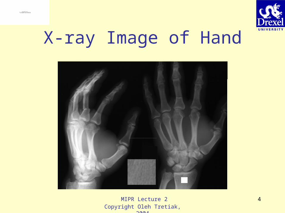
X-ray Image of Hand


5



X-ray Imaging: How it works.

X-ray shadow cast by an object Strength of shadow depends on composition and thickness.


6



CT (Computed Tomography)

CT Image of plane throughliver and stomach Projection image

from CT scans


7



Computer Tomography:How It Works

Only one plane is illuminated. Source-subject motion provides added information.


8



Functional Magnetic Resonance Imaging

From http://www.fmri.org/Picture naming task

Plane 3

Plane 6


9



Detected Signal in MRI

Spinning magnetization induces a voltage in external coils, proportional to the size of magnetic moment and to the frequency.

H0

ω0

s(t)


10



Ultrasound Imaging

Twin pregnancy during week 10


11



Ultrasound Scanner

• A picture is built up from scanned lines.

• Echosonography is intrinsically tomographic.

• An image is acquired in milliseconds, so that real time imaging is the norm.

Transducer travel

Object

Image


12



Single Photon Computed Tomography

Images on left show three sections through the heart.A radioactive tracer, Tc99m MIBI (2-methoxy isobutyl isonitride) is injected and goes to healthy heart tissue.


13



Collimator

Only rays that are normal to the camera surface are detected.


14



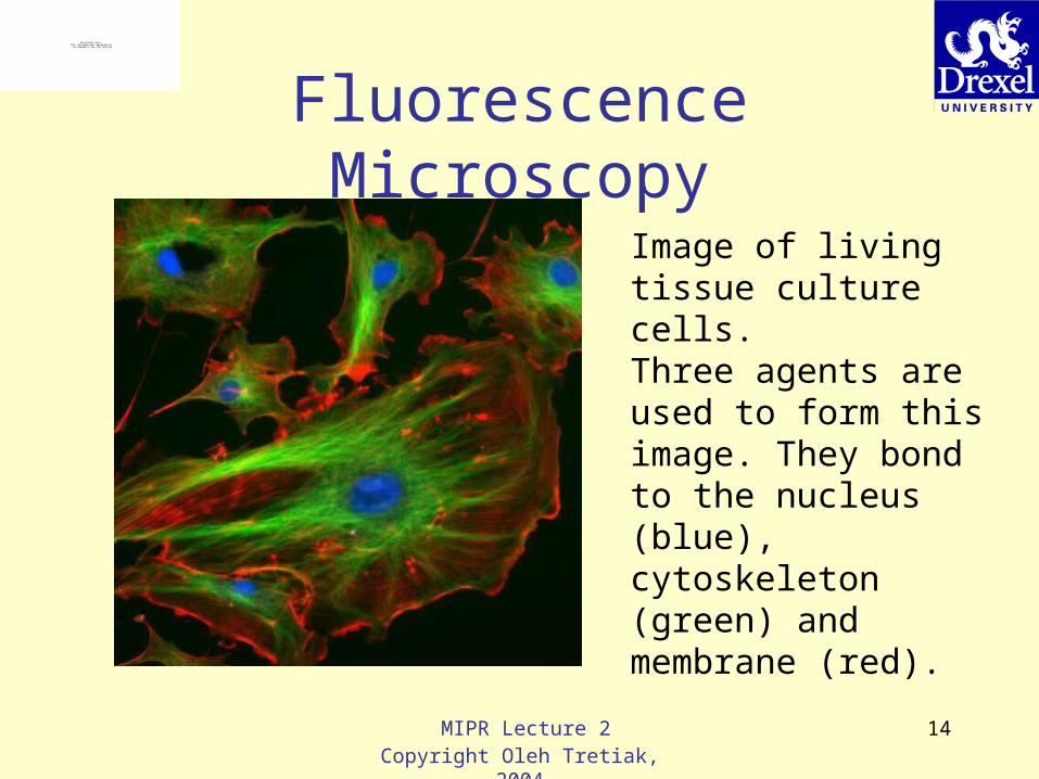
Fluorescence Microscopy

Image of living tissue culture cells. Three agents are used to form this image. They bond to the nucleus (blue), cytoskeleton (green) and membrane (red).


15



Modality ComparisonModality Strength Weakness Safety

X-Ray Simple, versatile

Only Air-Tissue-Bone Ionizing

CT Sectional Images

Low Resolution Ionizing

MRI Can see many properties

Slow Safe

Ultrasound Real timeOnly abdomen, limbs Safe

Isotope FunctionalSlow, low resolution Ionizing

Fluorescence Can see many properties

Low penetration Not applicable


16



Conclusions• Object - image - observer• Image should show the property of

concern– Fracture in bone– Blood flow to heart– Blood clot in brain

• No single best imaging method


17



This Lecture

• Fourier Analysis– Analysis of imaging systems– Measurement of imaging system

properties– Design of imaging system


18



Lesson Plan

• One-dimensional signals– Frequency decomposition– Fourier series– Signals and systems– Sampling– Quantization

• Two dimensions– Spatial frequencies– (Topics same as above)


19



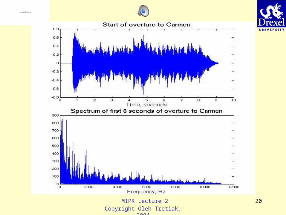
One-Dimensional Signals and Frequencies

• A signal can be a time function, s(t), but at the same time we think of it as being composed of many frequencies.

• AM radio– Signal (time function) received by an antenna– Radio waves contain many channels

• Music– Acoustic pressure waveform at a person’s ear– Combination of different notes


20




21



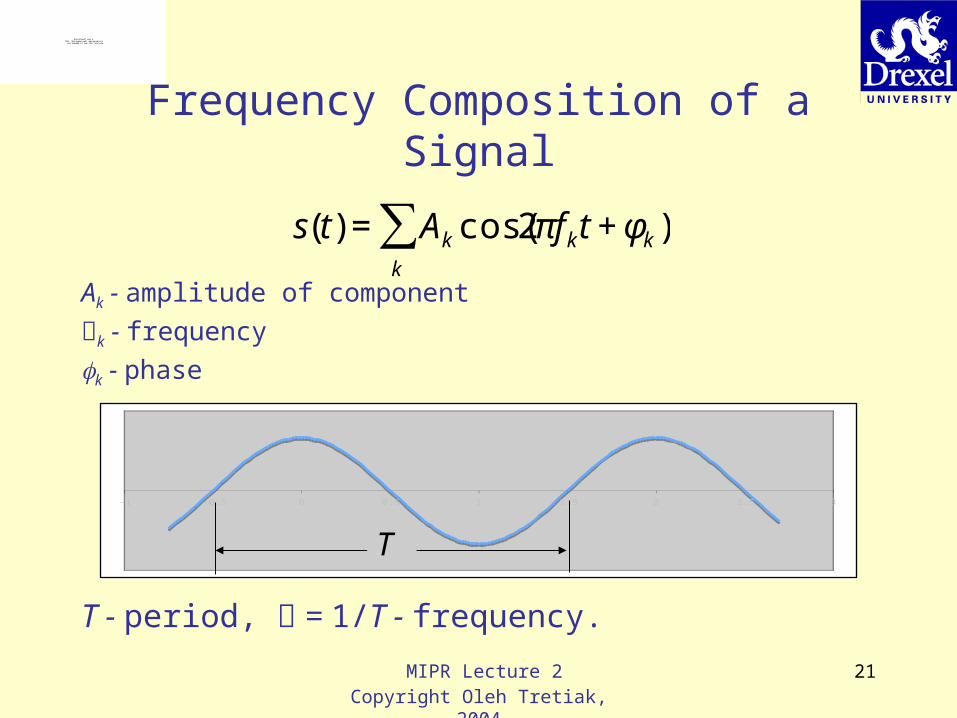
Frequency Composition of a Signal

Ak - amplitude of component

k - frequency

k - phase

T - period, = 1/T - frequency.

€

s(t) = Ak cos(2πfkt + φk )k

∑

-1 -0.5 0 0.5 1 1.5 2 2.5 3

T


22



Fourier Analysis

• Named after Josef Fourier, 1786-1830

• Basic idea: approximate function by a sum of sine/cosine functions

• Very powerful technique with many applications




23



Formula for Fourier Series

€

s(t) = A0 + Ak cos 2πkt /T( ) + Bk sin 2πkt /T( )( )k=1

∞

∑ , − T /2 < t < T /2

€

A0 =1

Ts(t)dt

−T / 2

+T / 2

∫ , Ak =2

Ts(t)cos 2πkt /T( )dt

−T / 2

+T / 2

∫ , k ≠ 0

Bk =2

Ts(t)sin 2πkt /T( )dt

−T / 2

+T / 2

∫

How to compute the Fourier Series coefficients:


24



Example of Fourier Approximation

Function

Fourier series, ca. 30 are nonzero

Sum of first 10 Fourier coeff. Not to good

Sum of first 20 Fourier coeff.Pretty good


25



Systems and Signal• Examples of signal reproducing systems:

– Sound systems• Telephone, Radio, Stereo

– Bioelectric activity• Electrocardiograms

– Bioacoustic system• Heart sounds

• System modeling– Input, system, output

hx(t) y(t)


26



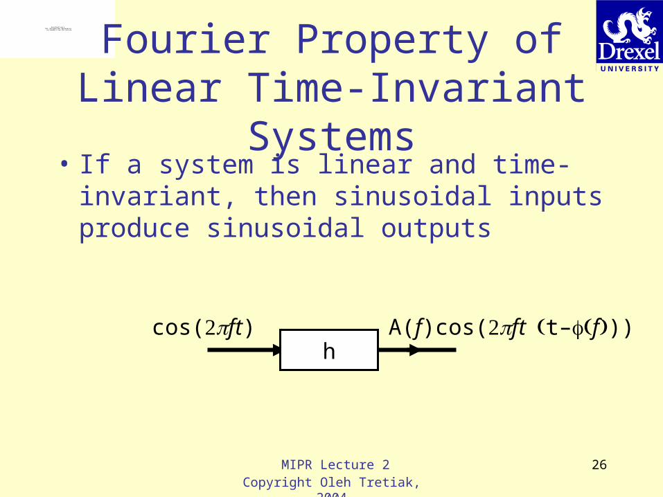
Fourier Property of Linear Time-Invariant Systems

• If a system is linear and time-invariant, then sinusoidal inputs produce sinusoidal outputs

hcos(ft) A(f)cos(ft t–f))


27



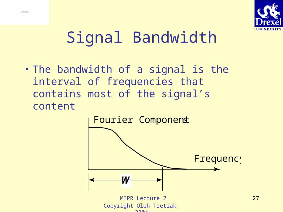
Signal Bandwidth

• The bandwidth of a signal is the interval of frequencies that contains most of the signal’s content

Frequency

Fourier Components


28



Example: Mystery Speech Signal


29



System Function and System Bandwidth

• Typical systems have a low-pass system function.

• W, the bandwidth of the system is the frequency range over which the system function is constant.

Frequency

System Function

W

Frequency

System Function

W Ideal low-pass filter


30



Bandwidth Theorem• The signal is faithfully reproduced if the signal

bandwidth is less than the system bandwidth

FrequencyInput Signal

System Function

Output Signal

FrequencyInput Signal

System Function

Output Signal

Adequate system bandwidth Inadequate bandwidth


31



Examples

• Conclusion: Speech is understandable if Wh ≥ 2 kHz

0.5 kHz

1.0 kHz

2.0 kHz

4.0 kHz


32



Digital Signal Processing• Most signals are processed digitally

– Example: mp3 encoding and playback of music, sound in cellular telephone

• The signal must be sampled

€

s(t), 0 < t < Tmax → s(kT0), 1 < k ≤ n = Tmax /T0

T0 ~ time between samples

f0 =1/T0 ~ sampling frequency or sampling rate

0 T 2T 3T TkT

f(T )

f(kT )f(3T )f(2T )


33



Sampling Theorem

• Frequency 2W is called the Nyquist sampling rate (Nyquist rate)

• A signal with no components at frequencies above W is called bandlimited.

• In practice, signals are approximately bandlimited.• In practice, we sample at a rate (1+a)2W. This is called

oversampling. 50% oversampling (a = 0.5) is simple and safe.

€

If x(t) has no components at frequency higher than W then it can be

recovered without error from samples taken at sampling rate f0 if

f0 > 2W .


34



Cardinal Series

• x(t) is a bandlimited signal, W is the bandwidth

• xs(k) = x(kT) is the sequence of samples.

€

xr(t) = x(kT)sin(π (t − kT) /T)

π (t − kT) /Tk=−∞

∞

∑

• If f0=1/T > 2W, then xr(t) = x(t)


35



Example of Cardinal Series

-0.5

0

0.5

1

1.5

2

-4 -3 -2 -1 0 1 2 3 4

f(-2) = 0.5, f(-1) = 1.0, f(0) = 1.5, f(1) = 1, f(2) = 0.5Sum of cardinal series is in black.


36



Two-Dimensional Fourier Analysis

€

s(u,v) = Ak cos(2π [ξ ku + η kv] + φk )k

∑

Two-dimensional frequency components of signal:

u, v are horizontal and vertical spatial coordinates, are horizontal and vertical spatial frequencies.If units of u, v are millimeters, units of are cycles per millimeter.


37



Space and Spatial Frequency

v u

€

f (u,v) = cos 2π (1× u + 2 × v)[ ]

ξ = u, η = v.

0.5 1.0


38



Example of 2D Fourier Transform

€

f (u,v) = exp(− | au | − | bv |)

€

ˆ f (ξ ,η ) =4 | ab |

(2πξ )2 + a2[ ] (2πη )2 + b2

[ ]

uv

Plots for a = 1, b = 2.


39



Examples of 2DFT

a

b

c

a

bc

Image Fouriertransform


40



Two-Dimensional Systems

• In analogy to one-dimensional systems, we use two-dimensional system models.

hx(u,v) y(u,v)

• If the system is linear and shift-invariant, when the input is sinewave, the output is also a sinewave.

€

If x(u,v) = cos(2π [ξu + ηv])

then y(u,v) =| H(ξ ,η ) | cos(2π [ξ ku + η kv] + φ(ξ ,η ))


41



‘Typical’ 2-D System Function

• The system function multiplies frequency component at spatial frequency .

• Typically, the response in the horizontal direction is different than the response in the vertical direction.

€

H(ξ ,η ) = exp −π (ξ /a)2 + (η /b)2[ ]{ }


42



Image and System Bandwidth

• Spatial bandwidth theorem– An image is reproduced faithfully if the

system function is constant for all frequencies present in the image.

In the example on the right, the frequency content in the x direction is greater than that in the h direction. The frequency content in the diagonal directions is smaller.


43



Examples of SystemsAdequate Bandwidth Inadequate Bandwidth


44



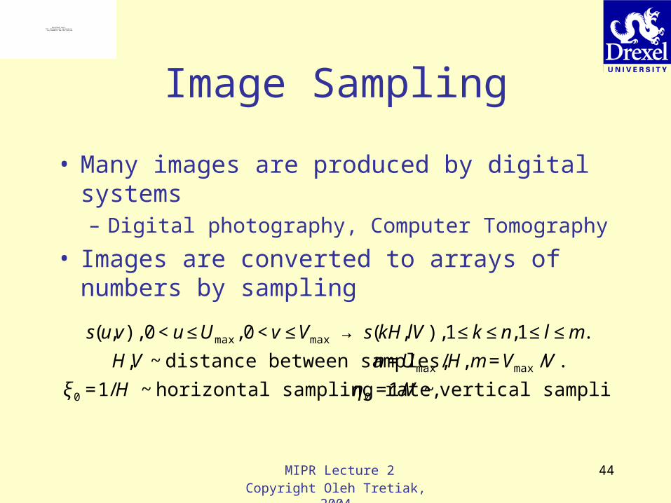
Image Sampling

• Many images are produced by digital systems– Digital photography, Computer Tomography

• Images are converted to arrays of numbers by sampling

€

s(u,v), 0 < u ≤ Umax , 0 < v ≤ Vmax → s(kH, lV ), 1≤ k ≤ n,1≤ l ≤ m.

H,V ~ distance between samples, n = Umax /H, m = Vmax /V .

ξ 0 =1/H ~ horizontal sampling rate, η 0 =1/V ~ vertical sampling rate.


45



2-D Sampling Pattern

u

v

H

V

x

h

x =1/H

h =1/V

Sampling grid in space

Sampling frequencies


46



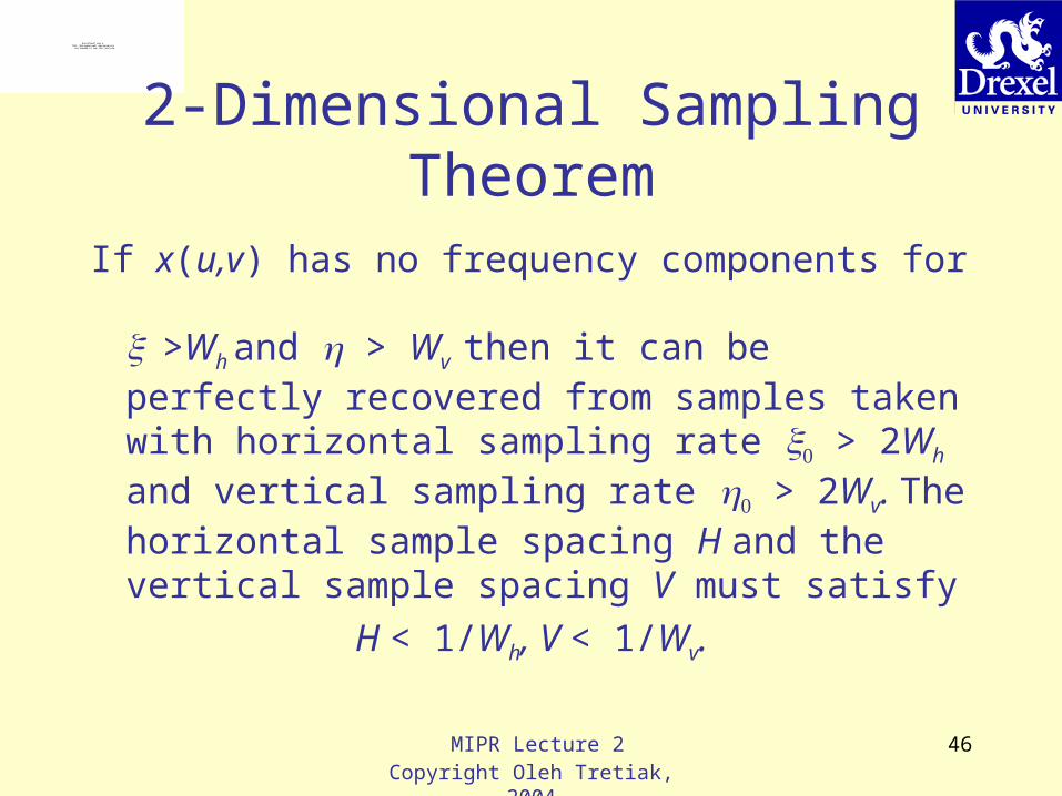
2-Dimensional Sampling Theorem

If x(u,v) has no frequency components for

>Wh and > Wv then it can be perfectly recovered from samples taken with horizontal sampling rate 0 > 2Wh and vertical sampling rate 0 > 2Wv. The horizontal sample spacing H and the vertical sample spacing V must satisfy

H < 1/Wh, V < 1/Wv.


47



2-Dimensional Sampling Theorem Diagram

x

h

h0> 2W

x0> 2W

W

W

Nonzero frequencies in the signal


48



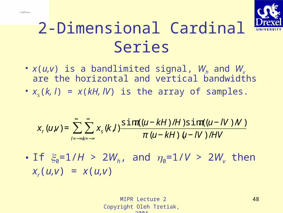
2-Dimensional Cardinal Series

• x(u,v) is a bandlimited signal, Wh and Wv are the horizontal and vertical bandwidths

• xs(k, l) = x(kH, lV) is the array of samples.

€

xr(u,v) = xs(k, l)sin(π (u − kH) /H)sin(π (u − lV ) /V )

π (u − kH)(u − lV ) /HVk=−∞

∞

∑l=−∞

∞

∑

• If 0=1/H > 2Wh, and 0=1/V > 2Wv then xr(u,v) = x(u,v)


49



Summary - Fourier Analysis

• Signals are composed of sinewaves (Fourier components).

• The effect of a linear time (or space)-invariant system is to multiply the components by factors that depend on frequency.

• These results apply in one and in two dimensions.

• In two dimensions, frequency is a vector (it has horizontal and vertical components).


50



Conclusions - more

• Signals and systems have bandwidth• If the system bandwidth is greater than

the signal bandwidth, the signal is accurately reproduced.

• If the system bandwidth is less than the signal bandwidth, the signal is distorted.

• In two dimensions, bandwidth is more interesting.


51



Concluding Conclusions

• If a signal is sampled at a high enough rate, it can be reproduced from the samples.

• The required sampling rate is twice the maximum frequency.

• In two dimensions, sampling rates in two directions be different.

Documents

MIPR Lecture 2 Copyright Oleh Tretiak, 2004 1 Medical Imaging and Pattern Recognition Lecture 2 Images and Fourier Analysis Oleh Tretiak