Mining SNPs from EST sequences using filters and ensemble

©FUNPEC-RP www.funpecrp.com.brGenetics and Molecular Research 9 (2): 820-834 (2010)

Mining SNPs from EST sequences using filters and ensemble classifiers

J. Wang1*, Q. Zou2* and M.Z. Guo1

1School of Computer Science and Technology, Harbin Institute of Technology, Harbin, Heilongjiang, P.R. China2School of Information Science and Technology, Xiamen University, Xiamen, Fujian, P.R. China

*These authors contributed equally to this study.Corresponding author: M.Z. GuoE-mail: [email protected]

Genet. Mol. Res. 9 (2): 820-834 (2010)Received January 11, 2010Accepted February 8, 2010Published May 4, 2010DOI 10.4238/vol9-2gmr765

ABSTRACT. Abundant single nucleotide polymorphisms (SNPs) provide the most complete information for genome-wide association studies. However, due to the bottleneck of manual discovery of putative SNPs and the inaccessibility of the original sequencing reads, it is essential to develop a more efficient and accurate computational method for automated SNP detection. We propose a novel computational method to rapidly find true SNPs in public-available EST (expressed sequence tag) databases; this method is implemented as SNPDigger. EST sequences are clustered and aligned. SNP candidates are then obtained according to a measure of redundant frequency. Several new informative biological features, such as the structural neighbor profiles and the physical position of the SNP, were extracted from EST sequences, and the effectiveness of these features was demonstrated. An ensemble classifier, which employs a carefully selected feature set, was included for the imbalanced training data. The sensitivity and specificity of our method both exceeded 80% for human genetic data in the cross validation. Our method enables detection of SNPs from the user’s own EST dataset and can be used on species for which there is no genome data. Our tests showed that this method can effectively guide

821


Mining SNPs from EST sequences

SNP discovery in ESTs and will be useful to avoid and save the cost of biological analyses.

Key words: Single nucleotide polymorphisms; Expressed sequence tag; Filter; Ensemble classifier; SNPDigger

INTRODUCTION

Recent studies have shown that genetic variation is the basis of genome-wide disease association research. Increasing attention has focused on the identification of human genetic variations. Single nucleotide polymorphisms (SNPs), which are small genetic changes or variations, occur at single-nucleotide positions within an individual’s DNA sequence. SNPs can characterize most of the genetic variations among different people. Compared with other genetic markers, such as microsatellites, SNPs are more common and may provide a high density of markers near a locus of interest. SNPs can be discovered from DNA fragmentary sequences, and are found on average at every 1 to 2 kb in the human genome (Clifford et al., 2000; Deutsch et al., 2001). SNPs in correlative DNA regions can provide considerable genetic information for genome-wide association studies, especially for genetic disease association research.

However, the cost of true SNP discovery is an important bottleneck for SNP analysis. It is costly and time-consuming to find and validate SNPs through manual biological experi-ments. Expressed sequence tags (ESTs), which are obtained from many different tissues of different individuals, are an important resource for identifying polymorphisms in transcribed regions. EST sequences can easily be obtained from EST databases, and the genetic varia-tion information obtained from EST sequences, such as mutation frequency, can help in SNP identification. A variety of computational approaches have been proposed for the discovery of novel SNP markers from ESTs.

Picoult-Newberg et al. (1999) first proposed mining SNPs from EST sequences. They selected SNPs from candidates using four filters. The four filters can eliminate false align-ments, gaps and base-calling errors. Taillon-Miller et al. (1998) did the same using overlap-ping genomic sequences. At the same time, Marth et al. (1999) developed POLYBAYES for SNPs discovery, which was based on a simple-machine learning method: Naive Bayes. After that, many researchers looked for ways to distinguish SNPs from sequence errors. Besides the filters, Batley et al. (2003) proposed two scores, which helped them find 264 SNP candidates in maize. Softwares and web servers were also developed for mining SNPs from data, includ-ing autoSNP (Barker et al., 2003), SEAN (Huntley et al., 2006), SNPServer (Savage et al., 2005), and SNPdetector (Zhang et al., 2005).

Here, we propose a new method to rapidly identify SNPs from EST data; it was implemented as SNPDigger. EST sequences are aligned and grouped, and four parameters are employed to provide a primary confidence measure for the SNP candidates. Several new informative biological features are extracted and employed in a complex machine learning method, an ensemble-based classifier, to obtain the true SNPs. To assess this method, we applied it to human, monkey, rat, and soybean EST data from UniGene. We found our method to be efficient at detecting SNPs in different EST sequences even if the species have no genome data.

822


J. Wang et al.

METHODS

SNP candidate selection

EST sequences usually have different lengths and correspond to different DNA re-gions. Thus, before SNP mining, the ESTs need to be aligned and grouped into several clus-ters, each corresponding to a single DNA region.

The EST sequences are first aligned and grouped by CAP3 (Huang and Madan, 1999), since CAP3 often produces fewer errors in consensus sequences than PHRAP. With CAP3, ESTs are divided into several contigs that correspond to EST clusters. After that, the SNPs are mined separately from these aligned EST contigs.

In order to find the true SNPs in EST sequences, the algorithm first needs to list all the SNP candidates. The SNP candidates are usually selected from the alignments of ESTs using a measure of redundant frequency. However, with only redundant frequency, the quality of SNP candidates may decrease when the ESTs in the contig are too few. Also, the noise, which is caused by errors associated with cloning, sequencing and alignment procedures, may also influence the selection procedure of SNP candidates and introduce interferential information for the next step for SNP identification (Irizarry et al., 2000). Thus, to improve the quality of the selected SNP candidates, we defined three other parameters together with the redundant frequency to construct four filters for the SNP candidate selection. The details of these four parameters are as follows.

1. fm: The redundant frequency of mutation in each locus. It can be calculated as:

fm = nmu / Nwhere N is the number of ESTs in the contig and nmu is the number of mutations at the related locus.

2. numes: The EST contig depth. The contig depth equals the amount of ESTs consti-tuting the contig. Insufficient ESTs in one contig may cause a lack of SNP candidate informa-tion. The influence of noise may be increased when the information on variation provided by ESTs is deficient.

3. fva: The valid allele ratio at each locus in alignments of ESTs. In the alignments of ESTs, there are usually a lot of invalid alleles at some loci, such as the gap (usually in the middle of ESTs), space (usually at the start or end of ESTs) and missing alleles. These in-valid alleles are produced by sequencing or alignment and reduce the information content of the locus. Lower valid allele ratios will cause an increasing in pseudo-SNPs in the results (a pseudo-SNP is a non-SNP site that is wrongly put into the candidate set). However, over strict elimination of the loci that contain invalid alleles too may cause the loss of true SNPs. Thus, fva is chosen as an important parameter to select SNP candidates.

(Equation 1)

(Equation 2)

where ngap is the number of gaps at the related locus, nspace is the number of spaces at the related locus, and nmiss is the number of the missing alleles at the related locus.

4. faa: The ambiguous allele frequency at each locus. Unlike invalid alleles, the am-biguous alleles are usually the uncertain alleles in the sequencing procedure, such as the allele

823



“W”; they correspond to one or two alleles in A, G, C, T. Excessive ambiguous alleles will cause uncertainty of the mutation allele and increase the difficulty in SNP mining. Thus, the locus that has an faa higher than the given value will be eliminated from the candidate set.

where nA, nG, nC, nT are the numbers of A, G, C, T at the related locus.These parameters are used to construct four filters. For each parameter in its related

filter, the algorithm sets a cut-off value by training or experience. The locus that has the param-eter value lower than the cut-off value (for fm, numes, fva) or larger than the cut-off value (for faa) is eliminated. The SNP candidate set is obtained from ESTs after these filtrations.

SNP identification

The SNP candidate set consists of true SNPs and pseudo-SNPs. The mining algorithm needs to distinguish the true SNPs from the pseudo-SNPs. True SNP identification can be trans-formed into a classification problem. The true SNPs correspond to positive samples and the pseu-do-SNPs correspond to negative samples. The mining algorithm needs to construct a classifier to partition the positive samples and the negative samples. There are two critical steps in the classify-ing procedure; one is the classifying feature selection and the other is the classifier construction.

A large set of structural and sequence features of SNPs in ESTs are investigated, including the common ones such as mutation frequency and the new ones, which are novel to this kind of study. We were particularly interested in the new features that are biologically informative. The most relevant features are described below.

1. Mutation frequency: The different mutation frequencies between the normal sites and the SNP sites have been a powerful feature for SNP mining. The higher the observed mu-tation frequency, the more likely the locus is associated with an SNP.

2. Residue conservation: A feature is defined to measure the level of sequence con-servation among the SNP candidate and its neighboring residue positions. The conservation score of a sequence position j is defined as the information content of the nucleotide frequency distribution at this position in a multiple sequence alignment.

(Equation 3)

(Equation 4)

where pi represents the frequency of allele type i at a given locus j.Thus, the residue conservation for an SNP candidate can be calculated as:

(Equation 5)

where n is the length of the residue sequence and m is the number of the neighboring locus of the observed SNP candidate in the residue sequence.

3. Physical position a: The sequencing errors tend to occur near the 5’ or 3’ ends of the ESTs rather than in the middle of the ESTs. This is due to the inherent limitations of sequenc-

824


J. Wang et al.

ing technology. The SNP candidates in the middle of the ESTs are more likely to be true SNPs than the other candidates that lie at the start or end of the ESTs. Thus, we define a new feature to describe this case. The physical position a of an SNP candidate is represented by the ratio of the distance between the candidate to the middle locus of ESTs.

(Equation 6)

where dc is the physical position of SNP candidate in the ESTs, and dl is the length of the ESTs.4. Physical position b: In one given contig not all ESTs have the same length; this fact

causes some EST sequences’ start or end sites to appear in the middle of the alignments. Thus, the mining algorithm computes the frequencies of spaces in the loci that are in a 10-bp region around the SNP candidate and uses them to describe the distance between a given site and the start or end of the ESTs in the given alignments. More spaces in a locus mean that this locus is nearer the start or end sites of ESTs. The distance between the candidate and the start or end of ESTs is measured by the highest space frequency on a locus in the given region around the SNP candidate.

(Equation 7)

where i is the locus related to the neighboring site around the SNP candidate j, nispace is the number of spaces at locus i and N is the number of ESTs at locus i. The higher this frequency is, the nearer the candidate is to the start or end of the ESTs.

5. Alignments of neighbor profiles: When many ambiguous alleles, gaps or spaces appear in the alignments of neighbor profiles, it usually means that the frequencies of sequence error and alignment error are very high in this region. Some SNP candidates in this region may be introduced by the noise. Thus, we calculate the number of loci that have frequencies of ambiguous alleles, gaps or spaces higher than given values in the neighbor profiles of the SNP candidate, and define this number as an important feature of SNP confirmation.

6. Mutation type: The cytosine in the CpG is very easily transformed to thymi-dine through methylation and deaminase activity (Holliday and Grigg, 1993). Thus, the frequency of transition is higher than the frequency of transversion. Almost 70.1% of the SNPs in the human genome are caused by transition (Mullikin et al., 2000). It means that the frequency of locus mutations including C/T and A/G is higher than the frequency of other mutations such as A/C and A/T. Therefore, we define a score for the feature of muta-tion type. The mutations such as C/T and A/G are given score value 1 and the other muta-tion types are given score value 0.

7. Content of nearby alleles: The allele content around the SNP candidates is also an important feature affecting the true SNP confirmation. SNPs are often discovered in regions that have unbalanced allele contents. If the contents of each allele in one region are almost at equilibrium, it usually means that there is no recombination happening in this region and the probability of finding SNPs in this region is very low. Thus, the allele contents in a 10-bp region around an SNP candidate are calculated, and are set to be an important feature for true SNP selection.

These seven kinds of features can be roughly divided into three classes: a) conser-vation: mutation frequency and residue conservation; b) physical and structural proper-

825



ties: physical position a, b and alignments of neighbor profiles, and c) sequence attributes: mutation type and content of nearby alleles. The valid SNPs in the ESTs have a special value in these features. Thus, we can construct some classifiers to identify the true SNPs in candidate set.

The supervised classifying procedure needs to construct a training model (classifier) from training data. In the case of SNP mining, the training data contain the aligned ESTs and the valid SNPs (the SNPs that are validated by biological experiments) in these ESTs. The SNP candidates, which are obtained from the training ESTs by the filters described in the “SNP Candidate Selection” Section, are separated as the negative set and the positive set. The positive set St contains all valid SNPs in an SNP candidate set. The negative set Sf contains the other sites in a candidate set. Since the valid SNPs only account for a small part of the SNP candidates, |St|<<|Sf|, we face a class imbalance problem. General classifiers usually use under-sampling technology to obtain class balanced training sets. However, under-sampling technol-ogy only chooses part of the training data to construct the new balanced training set and loses some information from the original training data. Thus, in our methodology, a novel algorithm is proposed to obtain a balanced training set and construct the classifying model from the training data without information loss. The algorithm details are described as follows:

1. Training data preprocessing: Sf is randomly rearranged and divided into several equal parts {Sf1, Sf2,…,Sfm}. For each part Sfi, |Sfi|≈|St|≈|Sf|/m. St is combined with each Sfi and a new training set group {Sn1,Sn2,…,Snm} is obtained, where Sni = St Sfi, i [1,m]. Each Sni is a balanced set.

2. Ensemble classifier construction: Using the new training sets, the algorithm con-structs an ensemble-based classifier to identify true SNPs. It is proved that the greater the difference between predictors, the better the performance the ensemble that is constructed by these predictors will have (“predictor” is equivalent to “classifier” in our methodology) (Krogh and Vedelsby, 1995). Then, the classifier employs several different types of predictors for classifying the native SNPs, including decision trees, Support Vector Machine, bagging, BFTree, Decorate, Logit Boost, Random Forest, and so on. Weka is used for implementation (Frank et al., 2004; Frank and Witten, 2005). The predictors are trained by different training sets. When a new SNP candidate set comes, each predictor separately predicts the true SNPs in this candidate set. Then, all results are ensembled to provide the final result by voting. The voting rate is discussed in the “Experimental Results on Human Data” Section.

Without parameter optimization, the training algorithm usually obtains several weak classifiers after a training procedure. Too many weak classifiers will reduce the accuracy of ensemble one. A general classifier usually employs Adaboost technology to train the classifier repetitively with the same data and accomplish parameter optimization. However, in the case of class imbalance, the training set is large and repetitive training will increase computation complexity. Thus, a new optimization strategy is employed in our algorithm. The classifier is trained one by one. Each classifier Ci is trained by a training set Sni. Then, Sni is reclassified by Ci. Fni is defined as the subset of Sni and Fni that contains all elements that are falsely classified by Ci. Fni is put into the training sets Sni+1, Sni+2 and is used to train the next two classifiers. For the last classifier Cm, its related Fnm is put into the training set Sn1; Sn2 of classifiers C1, C2, and C1, C2 will be retrained. This procedure will continue until the accuracies of two contiguous classifiers reache 100% or exceed a given threshold. The ensemble classifier construction procedure is shown in Figure 1.

826


J. Wang et al.

The repetitive training of false classified samples can optimize the classifiers and avoid the production of weak classifiers. Since only the false classified samples are put into the next two train-ing sets and retrained, this procedure can avoid the high computation complexity of repetitive train-ing on the whole training set. Since the false classified samples are trained by different classifiers, this can avoid the over-fitting that is caused by repetitive training of the same data on one classifier.

Evaluation method

The performance of our method can be evaluated by two parameters: the sensitivity (sn) and the specificity (sp).

Figure 1. The ensemble classifier construction: the black sites represent the false classified sites and the boundaries of positive class and negative class are marked with dotted lines in the training procedure. SNPs = single nucleotide polymorphisms; ESTs = expressed sequence tags.

(Equation 8)

where TP is the number of true positives (here, the valid ones in the SNPs, which are predicted to be true by our algorithm, are taken as true positives), TN is the number of true negatives and equals the number of pseudo-SNPs, which are predicted to be non-SNPs by the classifier; FP is the number of false positives and FN is the number of false negatives.

Implementation

We implement our SNP mining method as SNPDigger in Java. JDK 1.6 or higher is

(Equation 9)

827



needed for SNPDigger. SNPDigger can be used in any OS with JVM, including Windows, Linux, Unix, etc. The input EST sequences are first aligned and grouped by CAP3. The aligned EST contigs are put into the SNPDigger as input. SNPDigger offers a tool for the user to ob-tain the training model of our method. The training tool needs the EST sequences that aligned by CAP3 and the valid SNPs marked in these ESTs as the training data. SNPDigger also offers a training model from the analysis of Human ESTs (see Results and Discussion). The final result of SNPDigger is the marked SNPs in each EST contig.

The software and the related experimental results can be downloaded freely from http://nclab.hit.edu.cn/~zouquan/snpdigger/. The CAP3 assembly algorithm used for EST alignment can be downloaded from http://seq.cs.iastate.edu/download.html. All these soft-wares are available for non-commercial use.

RESULTS AND DISCUSSION

Data collection

We downloaded human EST sequences and three other species EST sequence sets from UniGene database (ftp://ftp.ncbi.nih.gov/repository/UniGene/), where ESTs have been clustered. The first 100 human EST clusters in the UniGene were chosen for the experiments, including 22,994 EST sequences. Fifty Macaca fascicularis (crab-eating macaque) EST clus-ters, 99 Rattus norvegicus (rat) EST clusters and 99 Glycine max (soybean) EST clusters were also chosen for the experiments. EST sequences were assembled by CAP3 and divided into several contigs. For each contig, the EST consensus sequences were located in their related genome by the BLAST (Altschul et al., 1997). The valid SNPs in these ESTs were determined through the dbSNP database (Sherry et al., 2001). Since there is no genome data for soybeans, no valid SNPs were proved for these soybean ESTs.

Experimental results for trade-off test

In the procedure of the SNP candidate selection, the determination of the threshold value of each filter parameter will influence the quality of the obtained SNP candidates. Thus, using the human data, we did some trade-off tests on SNPDigger to set the reasonable thresh-old value for each filter parameter.

1. fm: SNP is often defined as a site that has a frequency of mutation larger than 1%. To avoid pseudo-mutations caused by sequence errors, fm needs to be larger than 0.02 in SNPDigger. And only sites whose related mutations appear in at least two ESTs are considered in our method, since the sequencing errors rarely occur at the same locus at two or more EST sequences.

2. numes: We separately selected and analyzed the obtained SNP candidates for dif-ferent contig depths (Figure 2). The size of the SNP candidate set decreases with increasing contig depth, but the number of true SNPs increases. When the numes [8,15], the curve of the true SNP ratio is smooth, and the true SNP ratios are relatively high. Thus, we chose the threshold value of numes as 8 in our experiments to obtain enough SNP candidates and a relatively high true SNP ratio. The contigs that have less than 8 ESTs are not considered to mine SNPs.

828


J. Wang et al.

Figure 2. The results for different contig depths. A. The number of single nucleotide polymorphism (SNP) candidates for different contig depths. B. The number of true SNPs in candidate sets for different contig depths. C. The true SNP ratios in candidate sets for different contig depths.

3. fva: The SNP candidates are separately selected from given EST data using a differ-ent fva. The results are shown in Figure 3. There is a dramatic decline in SNP candidate number, but the true SNPs in the selected candidates only decrease slightly before the fva reaches 0.875. The highest ratio of true SNPs in the candidate sets is reached at the point fva = 1. Thus, the val-ue of fva is set within [0.875, 1]. In our experiments, fva of selected SNPs had to be larger than 0.875 to reach a balance between the number of SNP candidates and the ratio of true SNPs.

829



Figure 3. The results for different fva. A. The number of single nucleotide polymorphism (SNP) candidates for different fva. B. The number of true SNPs in SNP candidate sets for different fva. C. The true SNP ratios in candidate sets for different fva.

830


J. Wang et al.

4. faa: In the above candidate selection experiments, we set faa ≤0.10 to maximize the obtained SNP candidates. Here, we tested the given EST data using different values of faa (Figure 4). The SNP candidates and the true SNPs in the candidates increased with increasing faa until the value of faa reached 0.08. Thus, the value of faa is set within [0, 0.08]. In the final experiments, faa was set to 0, to make sure that no ambiguous alleles influenced the true SNP confirmation.

Figure 4. The results for different faa. A. The number of single nucleotide polymorphism (SNP) candidates for different faa. B. The number of true SNPs in SNP candidate sets for different faa. C. The true SNP ratios in candidate sets for different faa.

831



A total of 3910 candidate SNPs were selected from 22,994 human EST sequences, taking into account all four parameters.

Experimental results on human data

The human EST data were used to test the performances of the chosen features. The obtained SNP candidates are represented by the value sets of selected features, and SNPs are identified from candidate set using several classifiers separately. The candidate set obtained from the SNP candidate selection step is divided into two parts: the testing set and the training set, where 20% is selected randomly as the testing set and the others are used for training. The training set consists of the positive set that contains all valid SNPs in the training set and of the negative set that contains all the other sites in the training set. Here, the size of negative set is nearly 15 times larger than the positive set. Consequently, we divided the negative set into 15 different equal subsets, randomly. Then, each negative subset combines with the positive set and 15 new balanced training sets are generated. Each balanced training set is used for training a predictor. When a new candidate comes up for testing, the 15 different predictors vote for the final decision. The SNP candidate is recognized as a true SNP site only if more than 50% of the predictors confirm it as true. The final voting result is given by the ensemble predictor.

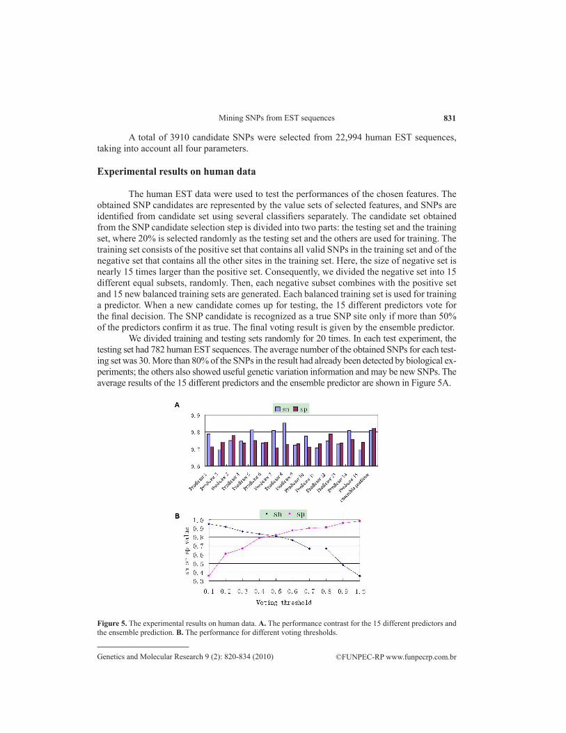
We divided training and testing sets randomly for 20 times. In each test experiment, the testing set had 782 human EST sequences. The average number of the obtained SNPs for each test-ing set was 30. More than 80% of the SNPs in the result had already been detected by biological ex-periments; the others also showed useful genetic variation information and may be new SNPs. The average results of the 15 different predictors and the ensemble predictor are shown in Figure 5A.

Figure 5. The experimental results on human data. A. The performance contrast for the 15 different predictors and the ensemble prediction. B. The performance for different voting thresholds.

832


J. Wang et al.

Figure 5B gives the performance of sn and sp with different voting rates. As we can see, increasing the voting rate can give accurate sp, but it sacrifices sn, and visa. When the voting rate is set at 0.5, sn and sp both have average accurate values. Thus, in our experiments, the vot-ing rate was set at 0.5, and the two measures for our performance sn and sp all exceeded 80%.

Experiments on other specie data

Besides the human EST sequences, we also tested our method on three other species EST sets to test the validity of our method on other species and on species with no genome data.

Our method gave 194 SNP candidates with the human model in 50 M. fascicularis EST clusters, and 63 SNPs were detected in 20 contigs. Our method also obtained 1144 SNP candidates with the human model in 99 Rattus norvegicus EST clusters and 291 SNPs were detected in 92 contigs. Among these SNPs detected, 41 monkey SNPs and 62 rat SNPs had been validated by biological experiments and can be queried in the dbSNP database. We can-not be sure about the other SNPs detected by our method, because SNP sites of monkeys and rats in dbSNP are not as abundant as for human DNA. However, they also have a good pos-sibility to be new SNPs that have not been detected until now. The experiments on monkey and rat ESTs prove that the training model can be used on any species; but they will get better performance with the same class, such as the human model used on the Primate ESTs.

We also detected SNPs in the soybean ESTs for which no genome data were avail-able; 512 SNP candidates with the human model in 99 soybean EST clusters and 159 SNPs were detected in 33 contigs. This demonstrates that our method also can be used on species for which there are no genome data.

Comparison with other methods

We compared our method with five popular SNP mining methods. The details of these methods are described in Table 1.

Software URL Note

POLYBAYES http://bioinformatics.bc.edu/marthlab/PyroBayes 454 pyrosequences are used as input, Bayesian-based methodSNPdetector http://lpg.nci.nih.gov Fluorescence-based resequencing are used as input, NQS used to identify high-quality sequence variationsssahaSNP http://www.sanger.ac.uk/Software/analysis/ssahaSNP/ Shotgun reads are used as input, shotgun reads are aligned to the finished genome sequence to detect SNPsSEAN http://zebrafish.doc.ic.ac.uk/Sean EST sequences are used as input, the redundancy of the SNPs and sequence identity in the surrounding aligned sequences are used as measuresSNPServer http://hornbill.cspp.latrobe.edu.au/snpdiscovery.html EST sequences used as input, autoSNP based

EST = expressed sequence tags; NQS = neighborhood quality stardard.

Table 1. The details of five single nucleotide polymorphism (SNP) mining softwares.

In the first three methods, POLYBAYES uses the pyrosequences from the 454 Life Sciences sequencing machines. A Bayesian inference engine is employed to calculate the prob-ability that a given site is polymorphic in these sequences. SNPdetector detects SNPs from the fluorescence-based resequencing. High-quality sequence variations are identified using neighborhood quality standard. Heterozygous genotypes are identified and the validity of all

833



SNPs is evaluated at the end of the process. SsahaSNP (Ning et al., 2005) detects homozygous SNPs and indels by aligning shotgun reads to the finished genome sequence. All three meth-ods use the DNA sequencing data from experiments, such as 454 pyrosequences and shotgun reads. The SNPs are detected through evaluation of sequence signal quality. However, in our method, the SNPs are mined from the EST sequences. Almost all the species EST data can be found freely in NCBI; this can save the cost of data analysis on high-throughput reads. Also, the training model in our method is widely applicable and can be set freely by users. The per-formance of our method can be improved by increasing valid training data. These advantages can make our method more convenient than the three methods described above.

Both SNPServer and SEAN detect SNPs from EST sequences, similar as in our sys-tem. SNPServer uses autoSNP to detect SNPs and indels in EST data. Redundancy is used to differentiate between candidate SNPs and sequence errors. For each candidate SNP, two measures of confidence, redundancy of the polymorphism at an SNP locus and co-segregation of the candidate SNP with other SNPs in the alignment, are calculated to obtain the real SNPs. SEAN also uses the redundancy of the SNP in an alignment as a measure of confidence, but it reinforces this with a measure of sequence identity in the surrounding aligned sequences. Compared with SNPServer and SEAN, our method generates four filters to eliminate the se-quence errors and select candidate SNPs. These filters make the candidate SNPs more reliable. For each candidate SNP, our method introduces more features to measure the confidence of SNPs, which greatly reduces the influence of alignment errors and makes the final results more accurate. We conclude that this is an effective tool to mine SNPs from EST sequences.

CONCLUSIONS

We propose a novel computational method for mining SNPs from EST sequences and provide the implementation SNPDigger for this method. Four parameters, which are related to the EST alignments and SNPs, are analyzed to optimize the result of SNP candidate selec-tion. Seven kinds of features are investigated to represent the SNP attributes in the ESTs. An ensemble classifier is trained and employed to select the true SNPs from the candidate set. The experimental results demonstrated the good performance of our method (sn and sp both exceeded 80%). In our method, all SNPs are directly detected from the ESTs, without a need for the corresponding genome data. The experiments on ESTs of different species demonstrate the validity of our method. This could be used for finding SNPs as genetic markers for species for which we have no genome data.

ACKNOWLEDGMENTS

Research supported in part by the Chinese Natural Science Foundation (grants #60932008 and #60871092) and the Natural Science Foundation of Heilongjiang Province in China (grant #ZJG0705).

REFERENCES

Altschul SF, Madden TL, Schaffer AA, Zhang J, et al. (1997). Gapped BLAST and PSI-BLAST: a new generation of protein database search programs. Nucleic Acids Res. 25: 3389-3402.

Barker G, Batley J, O’ Sullivan H, Edwards KJ, et al. (2003). Redundancy based detection of sequence polymorphisms in

834


J. Wang et al.

expressed sequence tag data using autoSNP. Bioinformatics 19: 421-422.Batley J, Barker G, O’Sullivan H, Edwards KJ, et al. (2003). Mining for single nucleotide polymorphisms and insertions/

deletions in maize expressed sequence tag data. Plant Physiol. 132: 84-91.Clifford R, Edmonson M, Hu Y, Nguyen C, et al. (2000). Expression-based genetic/physical maps of single-nucleotide

polymorphisms identified by the cancer genome anatomy project. Genome Res. 10: 1259-1265.Deutsch S, Iseli C, Bucher P, Antonarakis SE, et al. (2001). A cSNP map and database for human chromosome 21.

Genome Res. 11: 300-307.Frank E and Witten IH (2005). Data Mining: Practical machine learning tools and techniques. 2nd edn. Morgan Kaufmann,

San Francisco.Frank E, Hall M, Trigg L, Holmes G, et al. (2004). Data mining in bioinformatics using Weka. Bioinformatics 20: 2479-2481.Holliday R and Grigg GW (1993). DNA methylation and mutation. Mutat. Res. 285: 61-67.Huang X and Madan A (1999). CAP3: A DNA sequence assembly program. Genome Res. 9: 868-877.Huntley D, Baldo A, Johri S and Sergot M (2006). SEAN: SNP prediction and display program utilizing EST sequence

clusters. Bioinformatics 22: 495-496.Irizarry K, Kustanovich V, Li C, Brown N, et al. (2000). Genome-wide analysis of single-nucleotide polymorphisms in

human expressed sequences. Nat. Genet. 26: 233-236.Krogh A and Vedelsby J (1995). Advances in Neural Information Processing Systems 7. In: Neural Network Ensembles,

Cross Validation, and Active Learning (Krogh A and Vedelsby J, eds.). MIT Press, Cambridge, 231-238.Marth GT, Korf I, Yandell MD, Yeh RT, et al. (1999). A general approach to single-nucleotide polymorphism discovery.

Nat. Genet. 23: 452-456.Mullikin JC, Hunt SE, Cole CG, Mortimore BJ, et al. (2000). An SNP map of human chromosome 22. Nature 407: 516-520.Ning Z, Caccamo M and Mullikin JC (2005). ssahaSNP-A polymorphism detection tool by genomic alignment. Proceedings

of the 2005 IEEE Computational Systems Bioinformatics Conference - Workshops (CSBW’05), Stanford, 251-254.Picoult-Newberg L, Ideker TE, Pohl MG, Taylor SL, et al. (1999). Mining SNPs from EST databases. Genome Res. 9:

167-174.Savage D, Batley J, Erwin T, Logan E, et al. (2005). SNPServer: a real-time SNP discovery tool. Nucleic Acids Res. 33:

W493-W495.Sherry ST, Ward MH, Kholodov M, Baker J, et al. (2001). dbSNP: the NCBI database of genetic variation. Nucleic Acids

Res. 29: 308-311.Taillon-Miller P, Gu Z, Li Q, Hillier LD, et al. (1998). Overlapping genomic sequences: a treasure trove of single-

nucleotide polymorphisms. Genome Res. 748: 754.Zhang J, Wheeler DA, Yakub I, Wei S, et al. (2005). SNPdetector: a software tool for sensitive and accurate SNP detection.

PLoS. Comput. Biol. 1: e53.

Documents

Mining SNPs from EST sequences using filters and ensemble