Embed Size (px)
Citation preview

17
Mining Concept Sequences from Large-Scale Search Logsfor Context-Aware Query Suggestion
ZHEN LIAO, Nankai UniversityDAXIN JIANG, Microsoft Research AsiaENHONG CHEN, University of Science and Technology of ChinaJIAN PEI, Simon Fraser UniversityHUANHUAN CAO, University of Science and Technology of ChinaHANG LI, Microsoft Research Asia
Query suggestion plays an important role in improving usability of search engines. Although some recentlyproposed methods provide query suggestions by mining query patterns from search logs, none of them mod-els the immediately preceding queries as context systematically, and uses context information effectively inquery suggestions. Context-aware query suggestion is challenging in both modeling context and scaling upquery suggestion using context. In this article, we propose a novel context-aware query suggestion approach.To tackle the challenges, our approach consists of two stages. In the first, offline model-learning stage, toaddress data sparseness, queries are summarized into concepts by clustering a click-through bipartite. Aconcept sequence suffix tree is then constructed from session data as a context-aware query suggestion model.In the second, online query suggestion stage, a user’s search context is captured by mapping the query se-quence submitted by the user to a sequence of concepts. By looking up the context in the concept sequencesuffix tree, we suggest to the user context-aware queries. We test our approach on large-scale search logsof a commercial search engine containing 4.0 billion Web queries, 5.9 billion clicks, and 1.87 billion searchsessions. The experimental results clearly show that our approach outperforms three baseline methods inboth coverage and quality of suggestions.
Categories and Subject Descriptors: H.2.8 [Database Management]: Database Applications—Datamining
General Terms: Algorithms, Experimentation
Additional Key Words and Phrases: Query suggestion, context-aware, click-through data, session data
ACM Reference Format:Liao, Z., Jiang, D., Chen, E., Pei, J., Cao, H., and Li, H. 2011. Mining concept sequences from large-scale search logs for context-aware query suggestion. ACM Trans. Intell. Syst. Technol. 3, 1, Article 17(October 2011), 40 pages.DOI = 10.1145/2036264.2036281 http://doi.acm.org/10.1145/2036264.2036281
The research of E. Chen is supported in part by Natural Science Foundation of China (grant no. 61073110),and Research Fund for the Doctoral Program of Higher Education of China (20093402110017). The researchof J. Pei is supported in part by Natural Sciences and Engineer Research Council of Canada (NSERC)through an NSERC Discovery Grant, and by BCFRST Foundation Natural Resources and Applied Sciences(NRAS) Endowment Research Team Program. All opinions, findings, conclusions and recommendations inthis article are those of the authors and do not necessarily reflect the views of the funding agencies.Authors’ addresses: Z. Liao, College of Information Technical Science, Nankai University, Tianjin, China;D. Jiang (corresponding author), Microsoft Research Asia, Beijing, China; email: [email protected];E. Chen, College of Computer Science, University of Science and Technology of China; J. Pei, School ofComputer Science, Simon Fraser University; H. Cao, College of Computer Science, University of Scienceand Technology of China; H. Li, Microsoft Research Asia, Beijing, China.Permission to make digital or hard copies of part or all of this work for personal or classroom use is grantedwithout fee provided that copies are not made or distributed for profit or commercial advantage and thatcopies show this notice on the first page or initial screen of a display along with the full citation. Copyrightsfor components of this work owned by others than ACM must be honored. Abstracting with credit is permit-ted. To copy otherwise, to republish, to post on servers, to redistribute to lists, or to use any component ofthis work in other works requires prior specific permission and/or a fee. Permissions may be requested fromthe Publications Dept., ACM, Inc., 2 Penn Plaza, Suite 701, New York, NY 10121-0701 USA, fax +1 (212)869-0481, or [email protected]© 2011 ACM 2157-6904/2011/10-ART17 $10.00
DOI 10.1145/2036264.2036281 http://doi.acm.org/10.1145/2036264.2036281
ACM Transactions on Intelligent Systems and Technology, Vol. 3, No. 1, Article 17, Publication date: October 2011.

17:2 Z. Liao et al.
1. INTRODUCTION
The effectiveness of a user’s information retrieval from the Web largely dependson whether the user can raise queries properly describing the information need tosearch engines. Writing queries is never easy, partially because queries are typi-cally expressed in a very small number of words (two or three words on average)[Jansen et al. 1998] and many words are ambiguous [Cui et al. 2002]. To make theproblem even more complicated, different search engines may respond differently tothe same query. Therefore, there is no “standard” or “optimal” way to raise queries toall search engines, and it is well recognized that query formulation is a bottleneck is-sue in the usability of search engines. Recently, most commercial search engines suchas Google, Yahoo!, and Bing provide query suggestions to improve usability. That is,by guessing a user’s search intent, a search engine can suggest queries which maybetter reflect the user’s information need. A commonly used query suggestion method[Baeza-Yates et al. 2004; Beeferman and Berger 2000; Wen et al. 2001] is to find simi-lar queries in search logs and use those queries as suggestions for each other. Anotherapproach [Huang et al. 2003; Jensen et al. 2006] mines pairs of queries which areadjacent or co-occur in the same query sessions.
Although the existing methods may suggest good queries in some scenarios, noneof them models the immediately preceding queries as context systematically, and usescontext information effectively in query suggestions. Context-aware query suggestionis challenging in both modeling context and scaling up query suggestion using context.
Example 1.1 (Search Intent and Context). Suppose a user raises a query “gladia-tor”. It is hard to determine the user’s search intent, that is, whether the user isinterested in the history of gladiator, famous gladiators, or the film Gladiator. With-out looking at the context of search, the existing methods often suggest many queriesfor various possible intents, and thus result in a low accuracy in query suggestion.
If we find that the user submits a query “beautiful mind” before “gladiator”, it is verylikely that the user is interested in the film Gladiator. Moreover, the user is probablysearching the films played by Russell Crowe. The query context which consists of thesearch intent expressed by the user’s recent queries can help to better understand theuser’s search intent and make more meaningful suggestions.
In this article, we propose a novel context-aware approach for query suggestion bymining concept sequences from click-through data and session data. When a usersubmits a query q, our context-aware approach first captures the context of q, whichis reflected by a short sequence of queries issued by the same user immediately beforeq. The historical data are then checked to find out what queries many users often askafter q in the same context. Those queries become the candidates of suggestion.
There are two critical issues in the context-aware approach. First, how should wemodel and capture contexts well? Users may raise various queries to describe thesame information need. For example, to search for Microsoft Research Asia, queries“Microsoft Research Asia”, “MSRA” or “MS Research Beijing” may be formulated.Directly using individual queries to describe context cannot capture contexts conciselyand accurately.
To tackle this problem, we propose summarizing individual queries into concepts,where a concept consists of a small set of queries that are similar to each other. Usingconcepts to describe contexts, we can address the sparseness of queries and interpretusers’ search intent more accurately.
To mine concepts from queries, we use the URLs clicked by users as the featuresof the corresponding queries. In other words, we mine concepts by clustering queriesin a click-through bipartite. Moreover, to cover new queries not in the click-through
ACM Transactions on Intelligent Systems and Technology, Vol. 3, No. 1, Article 17, Publication date: October 2011.

Mining Concept Sequences from Search Logs for Context-Aware Query Suggestion 17:3
Fig. 1. The framework of our approach.
bipartite, we represent each concept by a URL feature vector and a term feature vector.We will describe how to mine concepts of queries and build feature vectors for conceptsin Section 3.
With the help of concepts, a context can be represented by a short sequence of con-cepts corresponding to the queries asked by a user in the current session. The nextissue is that, given a particular context, what queries many users often ask in thefollowing.
It is infeasible to search a huge search log online for a given context. We proposea context mining method which mines frequent contexts from historical sessions insearch logs. The frequent contexts mined are organized into a concept sequence suffixtree structure which can be searched quickly. The previous mining process is con-ducted offline. In the online stage, when a user’s input is received, we map the se-quence of queries into a sequence of concepts as the user’s search context. We thenlook up the context in the concept sequence suffix tree to find out the concepts to whichthe user’s next query most likely belongs, and suggest the most popular queries inthose concepts to the user. The details about mining sessions, building a concept se-quence suffix tree, and making query suggestions are discussed in Section 4.
Figure 1 shows the framework of our context-aware approach, which consists of twostages. The offline model-learning stage mines concepts from a click-through bipar-tite constructed from search logs, creates feature vectors for the concepts, and buildsa concept sequence suffix tree from the sessions in the logs. The online query sugges-tion stage maps user query sequences into a concept sequence, looks up the conceptsequence against the concept sequence suffix tree, finds the concepts that the user’snext query may belong to, and suggests the most popular queries in the concepts. Themajor contributions of this work are summarized as follows.
First, instead of mining patterns of individual queries which may be sparse, we sum-marize queries into concepts. A concept is a group of similar queries. Although miningconcepts of queries can be reduced to a clustering problem on a bipartite graph, thevery large data size and the “curse of dimensionality” pose great challenges. To tacklethese challenges, we develop a novel and effective clustering algorithm in linear timecomplexity. We further increase the scalability of the clustering algorithm through twoapproaches.
Second, there are often a huge number of patterns that can be used for query sugges-tion. Mining those patterns and organizing them properly for online query suggestion
ACM Transactions on Intelligent Systems and Technology, Vol. 3, No. 1, Article 17, Publication date: October 2011.
17:4 Z. Liao et al.
is far from trivial. We develop a novel concept sequence suffix tree structure to addressthis challenge.
Third, users raise new queries to search engines everyday. Most log-based querysuggestion methods cannot handle novel queries that do not appear in the historicaldata. To tackle this challenge, we represent each concept derived from the log data bya URL feature vector and a term feature vector. New queries can thus be recognized asbelonging to some concepts through the two types of feature vectors.
Fourth, we conduct extensive studies on a large-scale search log dataset which con-tains 4.0 billion Web queries, 5.9 billion clicks, and 1.87 billion query sessions. Weexplore several interesting properties of the click-through bipartite and illustrate sev-eral important statistics of the session data. The data set in this study is severalmagnitudes larger than those reported in previous work.
Last, we test our approach on the search log data. The experimental results clearlyshow that our approach outperforms three baseline methods in both coverage and qual-ity of suggestions.
The rest of the article is organized as follows. We first review the related work inSection 2. The clustering algorithm and the query suggestion method are described inSections 3 and 4, respectively. We report an empirical study in Section 5. The articleis concluded in Section 6.
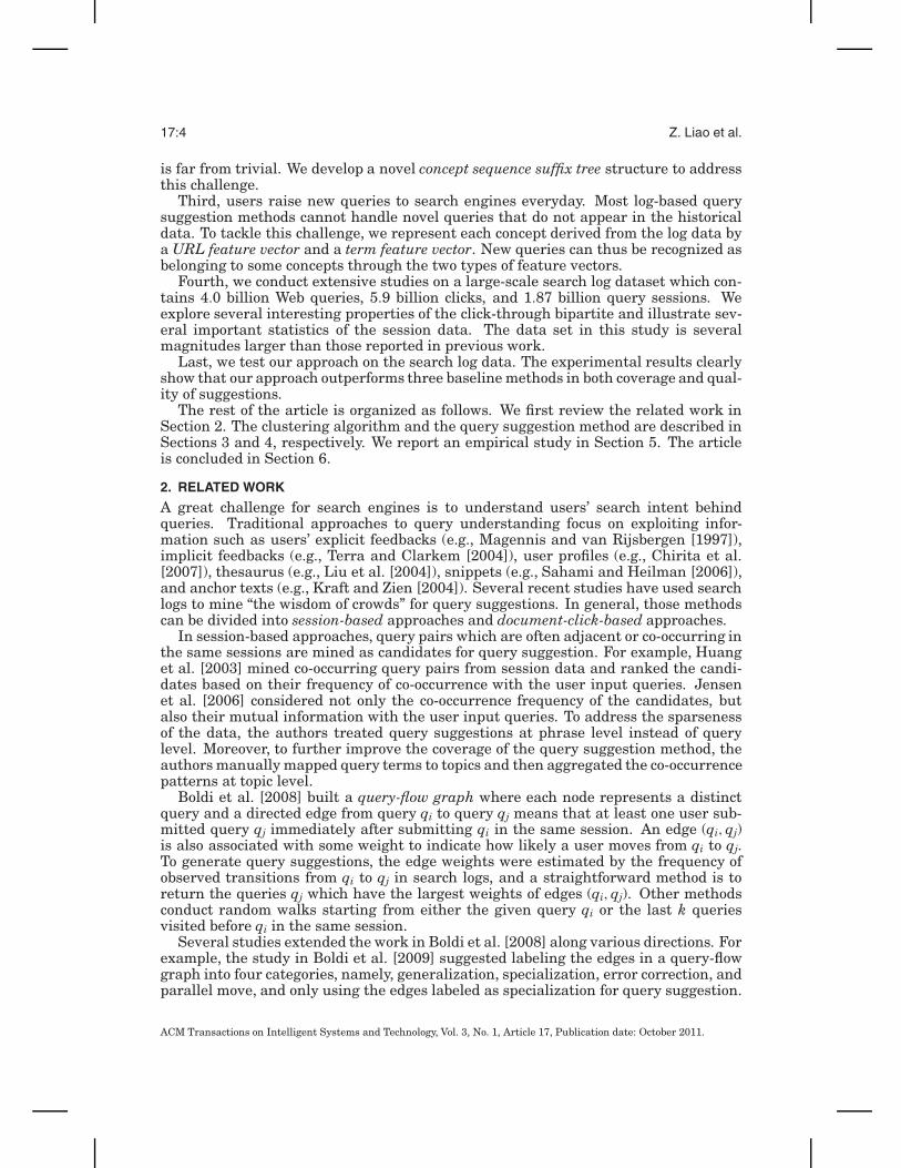
2. RELATED WORK
A great challenge for search engines is to understand users’ search intent behindqueries. Traditional approaches to query understanding focus on exploiting infor-mation such as users’ explicit feedbacks (e.g., Magennis and van Rijsbergen [1997]),implicit feedbacks (e.g., Terra and Clarkem [2004]), user profiles (e.g., Chirita et al.[2007]), thesaurus (e.g., Liu et al. [2004]), snippets (e.g., Sahami and Heilman [2006]),and anchor texts (e.g., Kraft and Zien [2004]). Several recent studies have used searchlogs to mine “the wisdom of crowds” for query suggestions. In general, those methodscan be divided into session-based approaches and document-click-based approaches.
In session-based approaches, query pairs which are often adjacent or co-occurring inthe same sessions are mined as candidates for query suggestion. For example, Huanget al. [2003] mined co-occurring query pairs from session data and ranked the candi-dates based on their frequency of co-occurrence with the user input queries. Jensenet al. [2006] considered not only the co-occurrence frequency of the candidates, butalso their mutual information with the user input queries. To address the sparsenessof the data, the authors treated query suggestions at phrase level instead of querylevel. Moreover, to further improve the coverage of the query suggestion method, theauthors manually mapped query terms to topics and then aggregated the co-occurrencepatterns at topic level.
Boldi et al. [2008] built a query-flow graph where each node represents a distinctquery and a directed edge from query qi to query qj means that at least one user sub-mitted query qj immediately after submitting qi in the same session. An edge (qi, qj)is also associated with some weight to indicate how likely a user moves from qi to qj.To generate query suggestions, the edge weights were estimated by the frequency ofobserved transitions from qi to qj in search logs, and a straightforward method is toreturn the queries qj which have the largest weights of edges (qi, qj). Other methodsconduct random walks starting from either the given query qi or the last k queriesvisited before qi in the same session.
Several studies extended the work in Boldi et al. [2008] along various directions. Forexample, the study in Boldi et al. [2009] suggested labeling the edges in a query-flowgraph into four categories, namely, generalization, specialization, error correction, andparallel move, and only using the edges labeled as specialization for query suggestion.
ACM Transactions on Intelligent Systems and Technology, Vol. 3, No. 1, Article 17, Publication date: October 2011.

Mining Concept Sequences from Search Logs for Context-Aware Query Suggestion 17:5
Anagnostopoulos et al. [2010] argued that providing query suggestions to users maychange user behavior. They thus modeled query suggestions as shortcut links on aquery-flow graph and considered the resulted graph as a perturbed version of theoriginal one. Then the problem of query suggestion was formalized as maximizing theutility function of the paths on the perturbed query-flow graph. Sadikov et al. [2010]extended the query-flow graph by introducing the clicked documents for each query.The queries q j following a given query qi are clustered together if they share manyclicked documents.
Unlike the preceding session-based methods which only focus on query pairs, wemodel various-length context of the current query, and provide context-aware sugges-tions. Although Boldi et al. [2008] and Huang et al. [2003] used the preceding queriesto prune the candidate suggestions, they did not model the sequential relationshipbetween the preceding queries in a systematic way. Moreover, most existing session-based methods focused on individual queries in context modeling and suggestion gen-eration. However, as mentioned in Section 1 (Introduction), user queries are typicallysparse. Consequently, the generated query suggestions could be very similar to eachother. For example, it is possible in a query-flow graph that two very similar queriesqj1 and q j2 are both connected to query qi with high weights. When q j1 and q j2 areboth presented to users as suggestions for qi, the user-perceived information wouldbe redundant. Although the method by Sadikov et al. [2010] grouped similar queriesin candidate suggestions, it cannot handle the sparseness of context. Our approachsummarizes similar queries into concepts and uses concepts in both context modelingand suggestion generation. Therefore, it is more effective to address the sparseness ofqueries.
The document-click-based approaches focus on mining similar queries from a click-through bipartite constructed from search logs. The basic assumption is that twoqueries are similar to each other if they share a large number of clicked URLs. Forexample, Mei et al. [2008] performed a random walk starting from a given query q onthe click-through bipartite to find queries similar to q. Each similar query qi is labeledwith a “hitting time,” which is essentially the expected number of random walk stepsto reach qi starting from q. The queries with the smallest hitting time were selectedas the query suggestions. Different from our method, the “hitting time” approach doesnot summarize similar queries into concepts. Moreover, it does not consider the con-text information when generating query suggestions. Other methods applied variousclustering algorithms to the click-through bipartite. After the clustering process, thequeries within the same cluster are used as suggestions for each other. For example,Beeferman and Berger [2000] applied a hierarchical agglomerative method to obtainsimilar queries in an iterative way. Wen et al. [2001] combined query content infor-mation and click-through information and applied a density-based method, DBSCAN[Ester et al. 1996], to cluster queries. These two approaches are effective to group sim-ilar queries. However, both methods have high computational cost and cannot scaleup to large data. Baeza-Yates et al. [2004] used the efficient k-means algorithm toderive similar queries. However, the k-means algorithm requires a user to specify thenumber of clusters, which is difficult for clustering search logs.
There are some other efficient clustering methods such as BIRCH [Zhang et al.1996] though they have not been adopted in query clustering. In BIRCH, thealgorithm constructs a Clustering Feature (CF for short) vector for each cluster.The CF vector consists of the number N of data objects in the cluster, the linearsum
−→LS of the N data objects, and the squared sum SS of the N data points. The
algorithm then scans the data set once and builds a hierarchical CF tree to indexthe clusters. Although the BIRCH algorithm is very efficient, it may not handle high
ACM Transactions on Intelligent Systems and Technology, Vol. 3, No. 1, Article 17, Publication date: October 2011.

17:6 Z. Liao et al.
dimensionality well. As shown in previous studies (e.g., Hinneburg and Keim [1999]),when the dimensionality increases, BIRCH tends to compress the whole dataset intoa single data item. In this article, we borrow the CF vector from BIRCH. However,to address the “curse of dimensionality” caused by the large number of URLs used asdimensions for queries in logs, we do not build CF trees. Instead, we develop the noveldimension array to leverage the characteristics of search log data.
The approach developed in this article also clusters similar queries using theclick-through bipartite. However, different from the previous document-click-basedapproaches which suggest queries from the same cluster of the current query, our ap-proach suggests queries that a user may ask in next step, which are more interestingthan queries simply replaceable to the current query.
To a broader extent, our method for query suggestion is also related to the methodsfor query expansion and query substitution, both of which also target at helping searchengine users to formulate good queries.
Query expansion involves adding new terms to the original query. Traditional IRmethods often select candidate expansion terms or phrases from pseudorelevance feed-backs. For example, Lavrenko and Croft [2001] created language models from thepseudorelevance documents and estimated the joint distribution P(t, q1, . . . , ql), wheret is a candidate term for expansion and q1, . . . , ql are the terms in the given query.Several other studies used machine learning approaches to integrate richer featuresin addition to term distributions. For example, Metzler and Croft [2007] applied aMarkov Random Field model and Cao et al. [2008] employed a Support Vector Ma-chine. Both approaches considered the co-occurrence as well as the proximity betweenquery terms and candidate terms. In recent years, several studies mined search logsfor query expansion. For example, Cui et al. [2002] showed that queries and documentsmay use different terms to refer to the same information. They built correlations be-tween query terms and document terms using the click-through information. Whenthe system receives a query q, all the document terms are ordered by their correlationto the terms in q, and the top terms are used for query expansion. Fonseca et al. [2005]proposed a method for concept-based interactive query expansion. For a query q, allthe queries which are often adjacent with q in the same sessions are mined as thecandidates for query expansion.
Query substitution alters the original query into a better form, for example, cor-recting spelling errors in the original query. In Guo et al. [2008], Jones et al. [2006],Lau and Horvitz [1999], Rieh and Xie [2001], and Silverstein et al. [1999], the authorsstudied the patterns how users refine queries in sessions and explored how to usethose patterns for query substitution. In Rieh and Xie 2001, the authors categorizedsession patterns into three facets, that is, content, format, and resource. For eachfacet, they further defined several subfacets. For example, within the content facet,the subfacets include specification, generalization, replacement with synonyms, andparallel movement. In Jones et al. [2006], the authors extracted candidates for querysubstitution from session data and built a regression model to calculate the confidencescore for each candidate. Guo et al. [2008] associated the query refinement patternswith particular operations. For example, for spelling correction, possible operations in-clude deletion, insertion, substitution, and transposition. The authors then treated thetask of query substitution as a structure prediction problem and trained a conditionalrandom field model from session data. Although many previous studies for query ex-pansion and query substitution are related to our work in the sense that they also useclick-through bipartite and session data, those methods have the following two essen-tial differences with our method. First, the methods for query expansion and querysubstitution aim at finding better formulation of the current query. In other words,they try to find queries replaceable to the current one. On the contrary, our query sug-
ACM Transactions on Intelligent Systems and Technology, Vol. 3, No. 1, Article 17, Publication date: October 2011.

Mining Concept Sequences from Search Logs for Context-Aware Query Suggestion 17:7
gestion method may not necessarily provide candidate queries which carry the samemeaning with the current one. Instead, it may provide suggestions that a user intendsto ask in the next step of the search process. Second, almost all the existing methodsfor query expansion and query substitution only focus on the current query pairs, whileour methods provide query suggestions depending on the context of the query. Whileconducting context-aware query expansion and substitution is an interesting researchproblem, we focus on on the problem of context-aware query suggestion in this article.
Another line of related work explored the effectiveness of using context informa-tion for predicting user interests. For example, White et al. [2010] assigned the topicsfrom the taxonomy created by the Open Directory Project1 to three types of contexts.The first type considered the preceding queries only, while the second and third typesadded clicked and browsed documents by the user. The authors confirmed that user in-terests are largely consistent within a session, and thus context information has goodpotential to predict the users short-term interests. In White et al. [2009], the authorsexplored various sources of contexts in browsing logs and evaluated their effectivenessfor the prediction of user interests. For example, besides the preceding pages browsedwithin the current session, the authors also considered the pages browsed in a long his-tory, the pages browsed by other users with the same interests, and so on. They founda combination of multiple contexts performed better than a single source. Mei et al.[2009] proposed using query sequences in sessions for four types of tasks, includingsequence classification, sequence labeling, sequence prediction, and sequence similar-ity. They found that many tasks, such as segmenting queries in sessions according touse interests, can benefit from context information. Although those previous studiesshowed the effectiveness of context information, none of them targeted at the particu-lar problem of query suggestion. Therefore, the techniques in those studies cannot beapplied or directly extended for our problem.
3. MINING QUERY CONCEPTS
In this section, we summarize queries into concepts. We first describe how to form aclick-through bipartite from search logs in Section 3.1. To address the sparseness of theclick-through bipartite, we perform a random walk on the graph. We then present anefficient algorithm in Section 3.2, which clusters the bipartite with only one scan of thedata. We further increase the scalability of the clustering algorithm by two approachesin Section 3.3. To improve the quality of clusters, we develop some postprocessingtechniques in Section 3.4. Finally, in Section 3.5, we derive concepts from clusters andconstruct a URL feature vector and a term feature vector for each concept.
3.1. Click-Through Bipartite
To group similar queries into a concept, we need to measure the similarity between twoqueries. When a user raises a query to a search engine, a set of URLs will be returnedas the answer. The URLs clicked by the user, called the clicked URL set of the query,can be used to approximate the information need described by the query. We can usethe clicked URL set of a query as the features of that query. The information aboutqueries and their clicked URL sets is available in search logs.
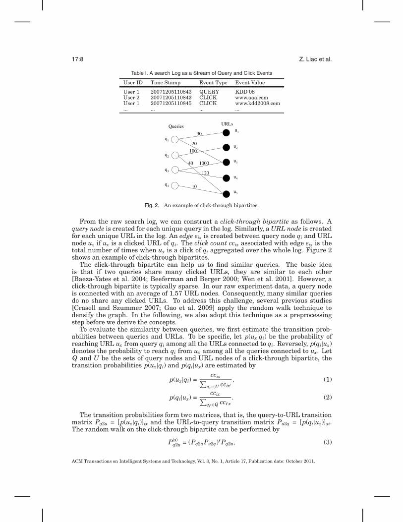
A search log can be regarded as a sequence of query and click events. Table I showsan example of a search log. In general, each row in a search log contains several fieldsto record a query or click event. From example, from Table I, we can read that ananonymous user 1 submitted query “KDD 08” at 11:08:43 on Dec. 5th, 2007, and thenclicked on URL www.kdd2008.com after two seconds.
1http://www.dmoz.org/
ACM Transactions on Intelligent Systems and Technology, Vol. 3, No. 1, Article 17, Publication date: October 2011.
17:8 Z. Liao et al.
Table I. A search Log as a Stream of Query and Click Events
User ID Time Stamp Event Type Event Value
User 1 20071205110843 QUERY KDD 08User 2 20071205110843 CLICK www.aaa.comUser 1 20071205110845 CLICK www.kdd2008.com... ... ... ...
Fig. 2. An example of click-through bipartites.
From the raw search log, we can construct a click-through bipartite as follows. Aquery node is created for each unique query in the log. Similarly, a URL node is createdfor each unique URL in the log. An edge eix is created between query node qi and URLnode ux if ux is a clicked URL of qi. The click count ccix associated with edge eix is thetotal number of times when ux is a click of qi aggregated over the whole log. Figure 2shows an example of click-through bipartites.
The click-through bipartite can help us to find similar queries. The basic ideais that if two queries share many clicked URLs, they are similar to each other[Baeza-Yates et al. 2004; Beeferman and Berger 2000; Wen et al. 2001]. However, aclick-through bipartite is typically sparse. In our raw experiment data, a query nodeis connected with an average of 1.57 URL nodes. Consequently, many similar queriesdo no share any clicked URLs. To address this challenge, several previous studies[Crasell and Szummer 2007; Gao et al. 2009] apply the random walk technique todensify the graph. In the following, we also adopt this technique as a preprocessingstep before we derive the concepts.
To evaluate the similarity between queries, we first estimate the transition prob-abilities between queries and URLs. To be specific, let p(ux|qi) be the probability ofreaching URL ux from query qi among all the URLs connected to qi. Reversely, p(qi|ux)denotes the probability to reach qi from ux among all the queries connected to ux. LetQ and U be the sets of query nodes and URL nodes of a click-through bipartite, thetransition probabilities p(ux|qi) and p(qi|ux) are estimated by
p(ux|qi) =ccix∑
ux′ ∈U ccix′, (1)
p(qi|ux) =ccix∑
qi′ ∈Q cci′x. (2)
The transition probabilities form two matrices, that is, the query-to-URL transitionmatrix Pq2u = [p(ux|qi)]ix and the URL-to-query transition matrix Pu2q = [p(qi|ux)]xi.The random walk on the click-through bipartite can be performed by
P(s)q2u = (Pq2uPu2q)sPq2u, (3)
ACM Transactions on Intelligent Systems and Technology, Vol. 3, No. 1, Article 17, Publication date: October 2011.

Mining Concept Sequences from Search Logs for Context-Aware Query Suggestion 17:9
where s is the number of steps of the random walk. When the number of s increases,more query-URL pairs will be assigned nonzero transition probabilities. In otherwords, the click-through bipartite becomes denser. However, a too large s may intro-duce noise and connect irrelevant query-URL pairs. In Gao et al. [2009], the authorsconducted an empirical study on different values of s and suggested a small value of 1to achieve high relevance between the connected query-URL pairs after random walk.We made consistent observations in our empirical study; we found more steps of ran-dom walk may bring in many small-weight edges between unrelated query-URL pairs.Therefore, we adopt the empirical value in Gao et al. [2009] and set s to a small valueof 1.
After the random walk, each query qi is represented as an L2-normalized vector,where each dimension corresponds to one URL in the bipartite. To be specific, the x-thelement of the feature vector of a query qi ∈ Q is
−→qiURL [x] = norm(wix) =
wix√∑ux′ ∈U w2
ix′
, (4)
where norm(·) is the L2 normalization function, and the weight wix of edge eix is definedas the transition probability from qi to ux after the random walk. If wix > 0, an edgewill be added between query qi and URL ux if it does not exist before the random walk.
The distance between two queries qi and q j is measured by the Euclidean distancebetween their normalized feature vectors. That is,
distanceURL(qi, q j) =√∑
ux∈U(−→qi
URL [x]−−→q jURL [x])2. (5)
Please note that we have to handle two types of data sparseness. First, the click-through bipartite is usually sparse in the sense that each query node is connected witha small number of related URLs, and vice versa. To address this problem, we apply therandom walk technique. Second, the user queries are also sparse since different usersmay refer to the same search intent using different queries. We handle this problemby summarizing queries into concepts in the following subsection.
3.2. Clustering Method
Now the problem is how to cluster queries effectively and efficiently in a click-throughbipartite. There are several challenges. First, a click-through bipartite from a searchlog is often huge. For example, the raw log data in our experiments consist of more than28.3 million unique queries. Therefore, the clustering algorithm has to be efficient andscalable to handle large datasets. Second, the number of clusters is unknown. Theclustering algorithm should be able to automatically determine the number of clusters.Third, since each distinct URL is treated as a dimension in a query vector, the datasetis of extremely high dimensionality. For example, the dataset used in our experimentsincludes more than 40.9 million unique URLs. Therefore, the clustering algorithmhas to tackle the “curse of dimensionality”. To the best of our knowledge, no existingmethods can address all the preceding challenges simultaneously. We develop a newmethod called the Query Stream Clustering (QSC) algorithm (see Algorithm 1).
In the QSC algorithm, a cluster C is a set of queries. The centroid of cluster C is
−→C URL [x] =
∑qi∈C−→qi
URL [x]
|C| , (6)
ACM Transactions on Intelligent Systems and Technology, Vol. 3, No. 1, Article 17, Publication date: October 2011.

17:10 Z. Liao et al.
ALGORITHM 1: Query Stream Clustering (QSC).Input: the set of queries Q and the diameter threshold Dmax;Output: the set of clusters � ;Initialization: dim array[d] = ∅ for each dimension d;1: for each query qi ∈ Q do2: C-Set = ∅;3: for each non-zero dimension d of −→qi
U RL do4: C-Set ∪= dim array[d];5: end for6: C = arg minC′∈C-Set distance(qi, C′);7: if diamter(C ∪ {qi}) ≤ Dmax then8: C ∪= {qi}; update the centroid and diameter of C;9: end if10: else C = new cluster({qi}); � ∪= C;11: for each non-zero dimension d of −→qi
U RL do12: if C /∈ dim array[d] then dim array[d] ∪ = {C};13: end for14: end for15: return �;
where |C| is the number of queries in C. The distance between a query q and a clusterC is given by
distanceURL (q, C) =√ ∑
ux∈U(−→q URL [x]−−→C URL [x])2. (7)
We adopt the diameter measure in Zhang et al. [1996] to evaluate the compactness ofa cluster, that is,
D = (
∑|C|i=1
∑|C|j=1(−→qi
URL −−→q jURL )2
|C|(|C| − 1))
12 . (8)
To control the granularity of clusters, we set a diameter parameter Dmax, that is, thediameter of every cluster should be smaller than or equal to Dmax.
The QSC algorithm considers the set of queries as a query stream and scans thestream only once. The query clusters are derived during the scanning process. Intu-itively, each cluster is initialized by a single query and then expanded gradually bysimilar queries. The expansion process stops when inserting more queries will makethe diameter of the cluster exceed the threshold Dmax. To be more specific, for eachquery q, we first find the closest cluster C to q among the clusters obtained so far, andthen test the diameter of C ∪ {q}. If the diameter is not larger than Dmax, q is assignedto C and C is updated to C∪{q}. Otherwise, a new cluster containing only q is created.
The potential major cost in our method is from finding the closest cluster for eachquery since the number of clusters can be very large. One may suggest to build a treestructure such as the CF-Tree in BIRCH [Zhang et al. 1996]. Unfortunately, as shownin previous studies (e.g., Hinneburg and Keim [1999]), the CF-Tree structure may nothandle high dimensionality well: when the dimensionality increases, BIRCH tends tocompress the whole dataset into a single data item.
How can we overcome the “curse of dimensionality” and find the closest cluster fast?We observe that the queries in the click-through bipartite are very sparse in dimen-sionality. For example, in our experimental data, a query is connected with an averagenumber of 3.1 URLs after random walk, while the average degree of URL nodes is only
ACM Transactions on Intelligent Systems and Technology, Vol. 3, No. 1, Article 17, Publication date: October 2011.

Mining Concept Sequences from Search Logs for Context-Aware Query Suggestion 17:11
Fig. 3. The data structure for clustering.
3.7. Therefore, for a query q, the average size of Qq, the set of queries which shareat least one URL with q, is only 3.1 · (3.7 − 1) = 8.37. Intuitively, for any cluster C, ifC ∩ Qq = ∅, C cannot be close to q since the distance of any member of C to q is
√2,
which is the farthest distance calculated according to Eq. (5) (please note the featurevectors of queries are normalized). In other words, to find out the closest cluster toq, we only need to check the clusters which contain at least one query in Qq. Sinceeach query belongs to only one cluster in the QSC algorithm, the average number ofclusters to be checked is not larger than 8.37.
Based on the previous idea, we use a dimension array data structure (Figure 3) tofacilitate the clustering procedure. Each entry of the array corresponds to one dimen-sion dx and links to a set of clusters �x, where each cluster C ∈ �x contains at leastone member query qi such that −→qi
URL [x] = 0. Given a query q, suppose the nonzerodimensions of −→q URL are d3, d6, and d9. To find the closest cluster to q, we only needto union the cluster sets �3, �6, and �9, which are linked by the third, sixth, andninth entries of the dimension array, respectively. Suppose �3 contains cluster C2, �6contains clusters C5 and C7, and �9 contains cluster C10. According to the precedingdiscussion, if q can be inserted into any existing cluster Ca, that is, the diameter ofCa ∪ {q} does not exceed Dmax, then Ca must belong to the union of �3, �6, and �9.Therefore, we only need to check whether q can be inserted into C2, C5, C7, and C10.Suppose q can be inserted C2 and C7, and the centroid of C7 is closer to q than that ofC2, we will insert q to C7. On the other hand, if q cannot be inserted into any clusterof C2, C5, C7, and C10, we will initialized a new cluster with q.
The QSC algorithm is very efficient since it scans the dataset only once. For eachquery qi, the number of clusters to be accessed is at most
∑dx∈NDi
|Qx|, where NDi
is the set of dimensions dx such that −→qiURL [x] = 0 and |Qx| is the number of queries
q j such that −→q jURL [x] = 0. As explained before, since the queries are sparse on di-
mensions in practice, the average sizes of both NDi and Qx are small. Therefore, thepractical cost for each query is constant, and the complexity of the whole algorithm isO(Nq), where Nq is the number of queries.
Our method needs to store the dimension array and the set of clusters. Since thecentroid and diameter of a cluster may be updated based on the feature vectors of themember queries during the clustering process, a naıve method would hold the featurevectors of the queries in clusters. In this case, the space complexity is O(Nu·Nq), whereNu and Nq are the numbers of URLs and queries, respectively.
To save space, we summarize a cluster Ca using a 3-tuple cluster feature[Zhang et al. 1996] (Nqa,
−−→LSa, SSa), where Nqa is the number of objects in the cluster,
ACM Transactions on Intelligent Systems and Technology, Vol. 3, No. 1, Article 17, Publication date: October 2011.

17:12 Z. Liao et al.
−−→LSa is the linear sum of the Nqa objects, and SSa is the squared sum of the Nqa objects.It is easy to show that the update of the centroid and diameter can be accomplishedby referring only to the cluster feature. In this way, the total space is reduced fromO(Nu · Nq) to O(Nu + Nq), where O(Nu) space is for dimension array and O(Nq) spaceis for the cluster feature vectors.
One might wonder that since the click-through bipartite is sparse, is it possible toderive the clusters by finding the connected components from the bipartite? To bespecific, two queries qi and q j are connected if there exists a query-URL path qi-ux1 -qi1 -ux2 -. . .-q j where adjacent query and URL in the path are connected by an edge. Acluster of queries can be defined as a maximal set of connected queries. An advantageof this method is that it does not need a specified parameter Dmax.
However, in our experiments, we find that although the bipartite is sparse, it ishighly connected. In other words, a large percentage (up to 50%) of queries, no mattersimilar or not, are included within a single connected component. Moreover, the pathbetween dissimilar queries cannot be broken by simply removing a few “hubs” of queryor URL nodes (please refer to Figure 12). This suggests the cluster structure of theclick-through bipartite is quite complex and we may have to use some parameters tocontrol the granularity of desired clusters.
Although Algorithm 1 is very efficient, the time and space cost can still be verylarge. Can we prune the queries and URLs without degrading the quality of clusters?We observe that edges with low weights (either absolute or relative) are likely to beformed due to users’ random clicks. Such edges should be removed to reduce noise.To be specific, let eix be the edge connecting query qi and ux, ccix be the click count ofeix, and wix be the weight of eix after the random walk. We can prune an edge eix ifccix ≤ τabs or wix ≤ τrel, where τabs and τrel are user-specified thresholds. After pruninglow-weight edges, we can further remove the query and URL nodes whose degreesbecome zero. In our experiments, we empirically set τabs = 5 and τrel = 0.05.
3.3. Increasing the Scalability of QSC
With the support of the dimension array, the QSC algorithm only needs to scan thedata once. However, the algorithm requires the dimension array to be held in mainmemory during the whole clustering process. In practice, a search log may containtens of millions unique URLs even after the pruning process. Holding the completedimension array in main memory becomes a bottleneck to scale up the algorithm. Toaddress this challenge, we develop two approaches. The first approach scans the dataiteratively on a single machine. During each scan, only a part of the dimension arrayneeds to be held in the main memory. The second approach applies distributed compu-tation under the master-slave programming model, where each slave machine holds apart of the dimension array in main memory.
3.3.1. Iterative Scanning Approach. In the QSC algorithm (Algorithm 1), each query iseither inserted into an existing cluster if the diameter of the cluster does not exceed thethreshold Dmax after insertion, or assigned to a newly created cluster otherwise. Thefirst case does not increase the memory consumption since we only need to update thevalue of the cluster feature of the existing cluster. However, the second case requiresextra memory to record the cluster feature for the new cluster. Therefore, a criticalpoint to control the memory usage of the QSC algorithm is to constrain the creation ofnew clusters.
Our idea is to adopt a divide-and-conquer approach and scan the query dataset inmultiple runs (see Figure 4). During each scan, only a part of the dimension array isheld in main memory. At the beginning, we scan the query dataset and process thequeries in the same way as in Algorithm 1. When the memory consumption reaches
ACM Transactions on Intelligent Systems and Technology, Vol. 3, No. 1, Article 17, Publication date: October 2011.

Mining Concept Sequences from Search Logs for Context-Aware Query Suggestion 17:13
Fig. 4. The idea of the iterative scanning approach.
the total size of the available machine memory, we stop creating new clusters. Forthe remaining queries in the dataset, we only try to insert them into the existingclusters. If a query cannot be inserted into any existing cluster, it will not be processedbut tagged as “unclustered.” After all queries in the dataset have been scanned, thealgorithm will output the clusters and release the memory for the current part of thedimension array.
Suppose the first scanning process stops creating new clusters at the M1-th query,that is, the M1-th query cannot be inserted into any existing cluster and the mem-ory consumption has reached the limit. The second run will continue with that M1-thquery and only process those unclustered queries. Again the second run of the scan-ning process stops creating new clusters when the memory limit is reached and onlyallows insertion operation for the remaining queries. This process continues until allthe unclustered queries are processed. This method is called Query Stream Clusteringwith Iterative Scanning (QSC-IS for short). The pseudocode is shown in in Algorithm 2.
ALGORITHM 2: Query Stream Clustering with Iterative Scanning (QSC-IS).Input: the set of queries Q, the diameter threshold Dmax and the memory limit L;Output: the set of clusters � on disk;Initialization: the position to start scanning M=0;1: while file end not reached do2: � =∅; dim array[d] = ∅ for each dimension d;3: seek to the M-th query;4: while (memory cost < L) && (file end not reached) do5: // process query as in Algorithm 1: until memory limit is reached or file ends6: read a query q into memory; M++;7: if q.state == “unclustered” then8: perform steps 3-10 of Algorithm 1:; q.state = “clustered”;9: end if10: end while11: while file end not reached do12: // continue scanning the file, but no new clusters are allowed to be created13: read a query q into memory;14: if q.state == “unclustered” then15: perform steps 3-7,9,10 of Algorithm 1:; q.state = “clustered”;16: end if17: end while18: Output � into disk;19: end while
ACM Transactions on Intelligent Systems and Technology, Vol. 3, No. 1, Article 17, Publication date: October 2011.

17:14 Z. Liao et al.
Fig. 5. The idea of the master-slave approach.
The main time cost of the QSC-IS algorithm is on multiple scans of the querystream. The number of scans depends on the memory limit. The larger the machinememory, the fewer runs needed. Let Nq be the number of queries and L be the totalnumber of scans. Suppose the ι-th (1 ≤ ι ≤ t− 1) scanning process stops creating newclusters at the Mι-th query, then the QSC-IS algorithm needs to scan a total numberof LNq −
∑L−1ι=1 (Mι − 1) queries. In our experiment, only 11 scans are needed by a 2G
memory machine for a dataset with 13.87 million queries (please refer to Section 5.2for details). Therefore, the complexity of QSC-IS is still considered as O(L · Nq) whereL� Nq.
The QSC-IS algorithm may generate different clustering results from those by theQSC algorithm (Algorithm 1). Suppose q can be inserted into both clusters Ca andCb , which are created in the first and second scan of the data, respectively. If Cb iscloser to q, the QSC algorithm will insert q into Cb , while the QSC-IS algorithm willinsert q into Ca, since Cb is not allowed to be created in the first scan of the data dueto memory limit. As we will discuss in Section 3.4, this problem can be addressed bysome postprocessing techniques.
3.3.2. Master-Slave Approach. When we have multiple machines, we can hold the di-mension array distributively under the master-slave programming model. As shownin Figure 5, each slave machine only holds a part of the dimension array and themaster machine determines on which slave machines a query should be processed.This method is called Query Stream Clustering in Master-Slave Model (or QSC-MS forshort). The pseudocode is presented in Algorithm 3.
Suppose there are M slave machines, we distribute the dimension array by thefollowing rule: the x-th entry of the dimension array is allocated to the (ω + 1)-th slavemachine if x mod M = ω. Under such a rule, the master machine can easily determinewhere to find the dimension array entry for any URL ux by a simple mode operationon M.
In the clustering process, the master machine reads each query q from the inputquery stream and identifies the set of URLs Uq with nonzero weights for q. For eachURL u ∈ Uq, the master determines the slave machine which stores the dimensionarray entry for u by the mode operation and dispatches (q, u) to that slave machinewith command “TEST”. The slave machine will look up the entry corresponding to u
ACM Transactions on Intelligent Systems and Technology, Vol. 3, No. 1, Article 17, Publication date: October 2011.

Mining Concept Sequences from Search Logs for Context-Aware Query Suggestion 17:15
ALGORITHM 3: Query Stream Clustering with Master-Slave Model (QSC-MS).Input: the set of queries Q, the number of slave machines M;
Output: the set of clusters � ;
Master Side: Host Program1: for each query q ∈ Q do2: for each non-zero dimension u of −→qi
URL do3: let k = u mod M;4: send message (q, u) with “TEST” to the k-th slave machine;5: end for6: receive a set of 〈cid, dia〉 tuples from the slave machines;7: if the smallest diameter diamin in the received tuples is -1 then8: let k= id of slave machine with maximal free memory;9: send message (q) with “CREATE” to the k-th slave machine;
10: receive the cluster-id cid from k-th slave machine;11: send message (q, cid) with “UPDATE” to the other slave machines;12: else13: find the cluster-id cidmin with the smallest diameter diamin;14: let k = id of slave machine which reports diamin;15: send message (q, cidmin) with “INSERT” to k-th slave machine;16: send message (q, cidmin) with “UPDATE” to the other slave machines;17: end if18: end for19: send command ”EXIT” to all slave machines.
Slave Side: Daemon Program
Input: the diameter threshold Dmax;
Initialization: dim array[d] = ∅;1: while true do2: if command == “TEST” then3: receive message (q, u);4: Cu← the set of clusters in the entry corresponding to u in dim array;5: if Cu = ∅ then6: get the minimum diameter diamin from cluster cidmin ∈ Cu;7: if diamin < Dmax then8: send message (cidmin, diamin) to the master machine;9: else
10: send message (−1,−1) to the master machine;11: end if12: else13: send message (−1,−1) to the master machine;14: end if15: end if16: if command == “INSERT” then17: received message (q, cid);18: add query q into cluster cid;19: update the cluster feature of cluster cid;20: end if21: if command == “CREATE” then22: received message (q);23: cid← cid + M;24: initialize new cluster cid with query q and send cid to master machine;25: end if26: if commend == “UPDATE” then27: received message (q, cid);28: for each nonzero dimension d of −→q do29: if d falls in this slave machine’s dim array then30: link cid to the corresponding entry;31: end if32: end for33: end if34: if command == “EXIT” then output clusters and exit the loop;35: end while
in its local dimension array, and retrieves a list of clusters Cu linked to the entry. Foreach cluster C ∈ Cu, the slave machine will test whether the insertion of q will make thediameter of C exceed the threshold Dmax. If q can be inserted into at least one cluster
ACM Transactions on Intelligent Systems and Technology, Vol. 3, No. 1, Article 17, Publication date: October 2011.

17:16 Z. Liao et al.
Fig. 6. The click-through bipartite for Example 3.1.
C ∈ Cu, the slave machine will pick up the closest cluster to q and send a response(cid, dia) to the master machine, where cid is the ID of the closest cluster and dia is thecorresponding diameter of the cluster if q is inserted. Otherwise, the response will be(−1,−1).
After the master machine receives all the replies from the slave machines, it willhandle two cases. In one case, all replies are (−1,−1). This means the current query qcannot be added into any existing cluster. For this case, the master machine identifiesthe slave machine with the maximal free memory and initializes a new cluster C withquery q on that slave machine by a message (q) with command “CREATE”.
In the other case, the current query q can be inserted into the closest existing clusterC with id cid. Suppose the cluster C locates on the k-th slave machine, the mastermachine will dispatch a message (q, cid) with command “INSERT” to the target slavemachine. The slave machine will update the cluster feature by incorporating the queryq into the cluster. Finally, the master machine will find out the nonzero URLs Uq andsend a message (u, cid) with command “UPDATE” for each u ∈ Uq to the correspondingslave machine. Each recipient slave machine will check the dimension array entry ofu and link cid to it if the link does not exist.
The major time expense of the QSC-MS algorithm is on network communication.Since network speed is usually far slower than disk scanning speed, the QSC-MS al-gorithm with ten slave machines is still slower than the QSC-IS algorithm on a singlemachine when they are compared on an experimental data with 13, 872, 005 queries(please refer to Section 5.2 and Figure 13). However, the QSC-MS algorithm requiresmuch less memory for an individual machine than the QSC-IS algorithm (please referto Section 5.2 and Figure 13).
3.4. Postprocessing of the Clusters
With the techniques presented in Section 3.3, the clustering algorithm can scale upto very large amounts of data. In this section, we target at improving the quality ofthe clusters. First, the QSC algorithm, as well as its extensions QSC-IS and QSC-MS,are order sensitive in that the clustering results may change with respect to the orderof the queries in the input stream. Such order sensitivity may result in low-qualityclusters. Second, the QSC family algorithms generate a hard clustering, which meansa query can only belong to one cluster. This requirement is not reasonable for multi-intent queries such as “gladiator” in Example 1.1. To better understand the theseaforesaid two problems, let us consider an example.
Example 3.1 (Order Sensitivity). Figure 6 shows a piece of click-through bipartitefrom a search log. In the search log, users who raised query “Roman gladiators”uniformly clicked on en.wikipedia.org/wiki/Gladiator. Consequently, the query“Roman gladiators” has a L2 normalized weight 1.0 on URL en.wikipedia.org/wiki/Gladiator. Moreover, users who raised query “Gladiator movie” mainly clickedon URL www.imdb.com/title/tt0172495, which is the IMDB site of the movie. At
ACM Transactions on Intelligent Systems and Technology, Vol. 3, No. 1, Article 17, Publication date: October 2011.
Mining Concept Sequences from Search Logs for Context-Aware Query Suggestion 17:17
Fig. 7. Two problems caused by the order sensitivity problem.
the same time, a few users might further explore some information about the glad-iators in the history, and they clicked on URL en.wikipedia.org/wiki/Gladiator.As a result, the query “Gladiator movie” has a normalized weight 0.9746 onURL www.imdb.com/title/tt0172495 as well as a normalized weight 0.2236 onen.wikipedia.org/wiki/Gladiator. The third query “gladiator” bears mixed intents.On the one hand, some users raised this query to find the information of Romangladiators, which resulted in a weight 0.6410 on en.wikipedia.org/wiki/Gladiator.On the other hand, some users intended to find the film Gladiator, which caused aweight 0.7675 on the URL www.imdb.com/title/tt0172495.
Now suppose we set the diameter threshold Dmax = 1. If the order of the threequeries in the input data is “Roman gladiators” � “Gladiator movie” � “gladiator”,where “q1 � q2” indicates query q1 appears before q2 in the input stream, then theclustering results will be C1 = {“Roman gladiators”} and C2 = {“gladiator”, “gladiatormovie”}. However, if the order becomes “gladiator” � “Roman gladiators”� “Gladiatormovie”, all the three queries will be assigned to the same cluster.
Ideally, “Roman gladiators” and “Gladiator movie” should be assigned to separateclusters while “gladiator” is assigned to both of them. However, the clustering re-sults of the QSC family algorithms are dependent on the order of queries. In someorders, such as “gladiator” � “Roman gladiators” � “Gladiator movie”, all the queriesare grouped in the same cluster. Even in the orders when “Roman gladiators” and“Gladiator movie” are assigned to separate clusters, since the algorithms generate ahard clustering, “gladiator” can only belong to one of them.
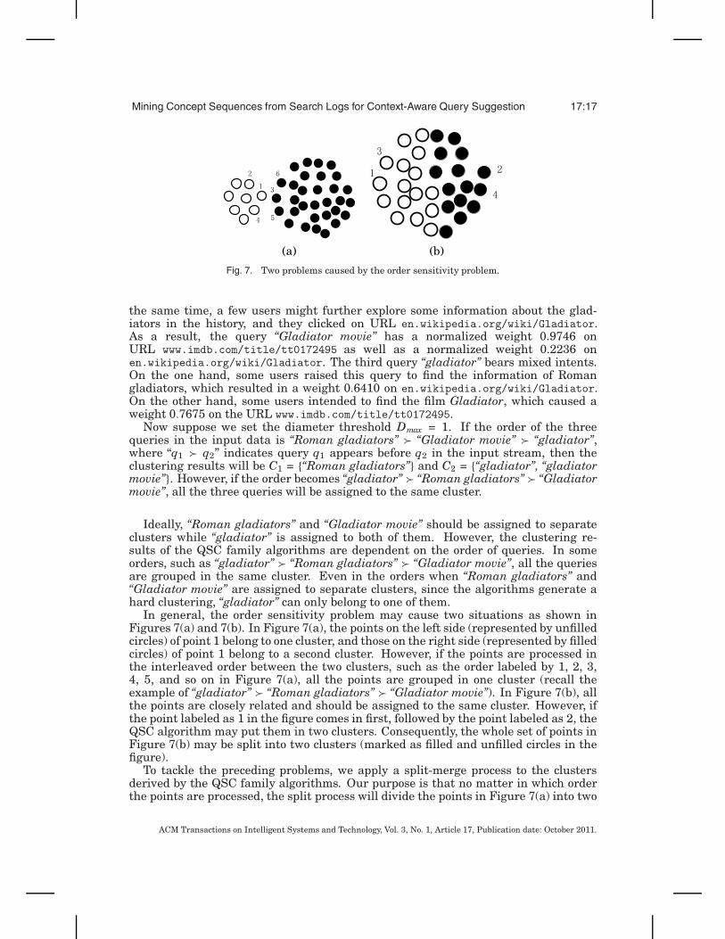
In general, the order sensitivity problem may cause two situations as shown inFigures 7(a) and 7(b). In Figure 7(a), the points on the left side (represented by unfilledcircles) of point 1 belong to one cluster, and those on the right side (represented by filledcircles) of point 1 belong to a second cluster. However, if the points are processed inthe interleaved order between the two clusters, such as the order labeled by 1, 2, 3,4, 5, and so on in Figure 7(a), all the points are grouped in one cluster (recall theexample of “gladiator” � “Roman gladiators” � “Gladiator movie”). In Figure 7(b), allthe points are closely related and should be assigned to the same cluster. However, ifthe point labeled as 1 in the figure comes in first, followed by the point labeled as 2, theQSC algorithm may put them in two clusters. Consequently, the whole set of points inFigure 7(b) may be split into two clusters (marked as filled and unfilled circles in thefigure).
To tackle the preceding problems, we apply a split-merge process to the clustersderived by the QSC family algorithms. Our purpose is that no matter in which orderthe points are processed, the split process will divide the points in Figure 7(a) into two
ACM Transactions on Intelligent Systems and Technology, Vol. 3, No. 1, Article 17, Publication date: October 2011.

17:18 Z. Liao et al.
clusters, while the merge process will group all the points in Figure 7(b) into a singlecluster.
In the split-merge process, we apply the Cluster Affinity Search Technique Algo-rithm (CAST) [Ben-Dor et al. 1999] to each cluster derived by the QSC family algo-rithms. In other words, we first apply the QSC family algorithm to the full querydataset and derive the query clusters. Then, we apply the CAST algorithm to eachderived cluster as a postprocessing step.
The basic idea of the CAST algorithm is to start with an empty cluster and graduallygrow the cluster each time with the object (i.e., query) that has the largest averagesimilarity to the current cluster. The growing process stops until the largest averagesimilarity to the current cluster is below a threshold σmin. At this point, the algorithmwill pick up the point in the current cluster which has the lowest average similarityσ with the current cluster and remove this point if σ < σmin. The algorithm iteratesbetween the growing and removing processes until no object can be added or removed.Then, the algorithm will output the current cluster and start to grow the next one.This process continues until all the objects have been processed.
The CAST algorithm, on the one hand, is quite similar to the QSC family algorithmsbecause both approaches use the average similarity or distance to control the granu-larity of clusters. One can easily verify that when the weights of queries −→q URL isL2 normalized, the thresholds adopted by the two approaches have the relationshipDmax =
√2(1− σmin).
On the other hand, the CAST algorithm has several critical differences with theQSC family algorithms. First, compared with the QSC family algorithms where theobjects are processed in the fixed order by the input stream, the CAST algorithm de-termines the sequence of objects to added into a cluster based on their similarity tothe cluster. Second, the CAST algorithm may adjust the current cluster by moving outsome objects, while the QSC family algorithms have no chance to correct their previousclustering decisions. Due to the preceding two differences, the CAST algorithm mayimprove the quality of the clusters derived by the QSC family algorithms. Please notethe quality improvement is obtained at the cost of higher computation complexity. Asdescribed in Ben-Dor et al. [1999], the computation complexity of the CAST algorithmis O(N2), while the complexity of the QSC family algorithms is only O(N), where Nis the number of objects to be clustered. Clearly, it is impractical to apply the CASTalgorithm to the whole query stream. However, in the postprocessing stage, we onlyapply the CAST algorithm to the clusters derived by the QSC family algorithms. Inpractice, the number of queries of the same concept is usually small. For example,in our experiment data, the largest clusters derived from the QSC family algorithmscontain 6,684 queries. Therefore, we can load each cluster derived by the QSC familyalgorithms into the main memory and apply the CAST algorithm efficiently.
After the split process, we merge two clusters if the diameter of the merged clusterdoes not exceed Dmax. In fact, the merge process can be considered as a second-orderclustering process, in which the query clusters instead of the individual queries areclustered. Naturally, we can reuse the dimension array structure and perform themerge process at O(Nc) time, where Nc is the number of clusters.
To allow a multi-intent query such as “gladiator” belong to two clusters, we apply areassignment process. To be specific, we check for each query q in cluster Ca whetherit can be inserted to another cluster Cb without making the diameter of Cb exceedDmax. If so, we call q is reassignable to Cb . Again, we maintain the dimension arraystructure and only check those clusters having common nonzero dimensions with q.Let Qb be the set of reassignable queries to cluster Cb . We first sort the queries inQb in the ascending order of their similarity to the centroid of Cb and then insert thequeries into Cb one by one. The insertion process stops when: (a) all the queries in Qb
ACM Transactions on Intelligent Systems and Technology, Vol. 3, No. 1, Article 17, Publication date: October 2011.

Mining Concept Sequences from Search Logs for Context-Aware Query Suggestion 17:19
have been inserted; or (b) the insertion of a query q in the sorted list makes the diam-eter of Cb exceed Dmax. In the latter case, the last query q will be removed from Cb .In our empirical study, among all the clusters with at least one reassignable queries,60% have exactly one reassignable query. According to the definition of reassignablequeries, those 60% cases trivially fall into the preceding category (a). In more generalcases, 98% of the clusters with at least one reassignable queries fall into category (a).Therefore, our reassignment process is robust to the order of queries. To be more spe-cific, our reassignment process is independent of the order of queries in the input datastream, since we specify a fixed order (similarity to the centroid of clusters) for them.We may choose other orders to insert the reassignable queries. However, differentorders will only affect 2% of the clusters with at least one reassignable queries.
Let us review Example 3.1 of queries “Roman gladiators”, “gladiator”, and “Gladi-ator movie”. We can verify no matter in which order these three queries appear, thesplit and merge process will put “Roman gladiators” and “Gladiator movie” separatelyin two clusters. After the reassignment process, we get two clusters: {“Roman gladia-tors”, “gladiator”} and {“Gladiator movie”, “gladiator”}.
3.5. Building Concept Features
Now we have derived a set of high-quality clusters from the click-through bipartite,where each cluster represents a concept. In the online stage of query suggestion, usersmay raise new queries which are not covered by the log data. To handle such newqueries, we create two feature vectors for each cluster. Let C be a cluster, and c be thecorresponding concept. The URL feature vector for c, denoted by −→c URL , is simply thecentroid of C defined in the URL space (Eq. (6)) , that is,
−→c URL [x] =−→C URL [x] =
∑qi∈C−→qi
URL [x]
|C| , (9)
where |C| is the number of queries in C. Analogously, we create a term feature vectorfor c based on the terms of the queries in C. To be specific, for each query qi ∈ C, wecan represent qi by its terms with the following formula
−→qiterm[t] = norm(tf (t, qi) · icf (t)), (10)
where norm(·) is the L2 normalization function, tf (t, qi) is the frequency of term t in qi,icf (t) = log Nc
Nc(t)is the inverse cluster frequency of t, Nc is number of clusters and Nc(t)
is number of clusters which contain queries with t. Then the term feature vector forconcept c is defined by
−→c term[t] =
∑qi∈C−→qi
term[t]
|C| . (11)
We will describe how to use these two features vectors to handle new queries at theonline stage in Section 4.3.
4. GENERATING QUERY SUGGESTIONS
In this section, we first introduce how to derive session data from search logs. Wethen develop a novel structure, concept sequence suffix tree, to summarize the patternsmined from session data. Finally, we present the query suggestion method based onthe mined patterns.
ACM Transactions on Intelligent Systems and Technology, Vol. 3, No. 1, Article 17, Publication date: October 2011.
17:20 Z. Liao et al.
Fig. 8. The procedure of building search and query session data.
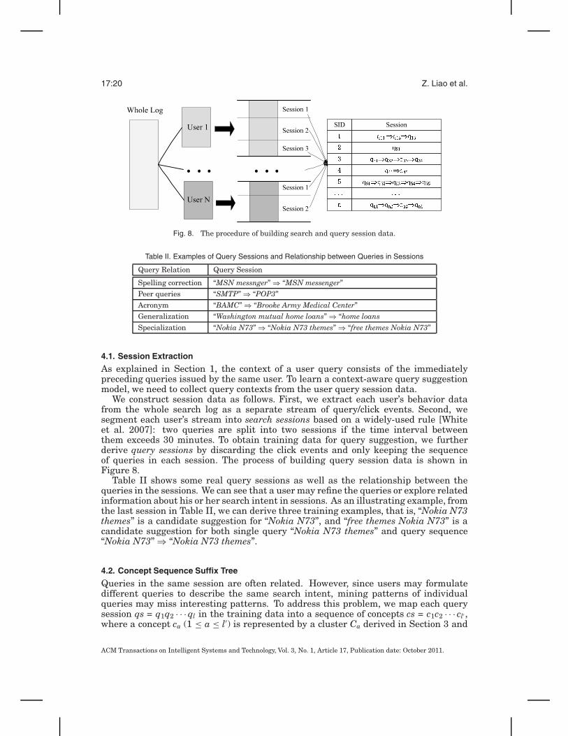
Table II. Examples of Query Sessions and Relationship between Queries in Sessions
Query Relation Query Session
Spelling correction “MSN messnger”⇒ “MSN messenger”Peer queries “SMTP”⇒ “POP3”
Acronym “BAMC”⇒ “Brooke Army Medical Center”Generalization “Washington mutual home loans”⇒ “home loans
Specialization “Nokia N73”⇒ “Nokia N73 themes”⇒ “free themes Nokia N73”
4.1. Session Extraction
As explained in Section 1, the context of a user query consists of the immediatelypreceding queries issued by the same user. To learn a context-aware query suggestionmodel, we need to collect query contexts from the user query session data.
We construct session data as follows. First, we extract each user’s behavior datafrom the whole search log as a separate stream of query/click events. Second, wesegment each user’s stream into search sessions based on a widely-used rule [Whiteet al. 2007]: two queries are split into two sessions if the time interval betweenthem exceeds 30 minutes. To obtain training data for query suggestion, we furtherderive query sessions by discarding the click events and only keeping the sequenceof queries in each session. The process of building query session data is shown inFigure 8.
Table II shows some real query sessions as well as the relationship between thequeries in the sessions. We can see that a user may refine the queries or explore relatedinformation about his or her search intent in sessions. As an illustrating example, fromthe last session in Table II, we can derive three training examples, that is, “Nokia N73themes” is a candidate suggestion for “Nokia N73”, and “free themes Nokia N73” is acandidate suggestion for both single query “Nokia N73 themes” and query sequence“Nokia N73”⇒ “Nokia N73 themes”.
4.2. Concept Sequence Suffix Tree
Queries in the same session are often related. However, since users may formulatedifferent queries to describe the same search intent, mining patterns of individualqueries may miss interesting patterns. To address this problem, we map each querysession qs = q1q2 · · · ql in the training data into a sequence of concepts cs = c1c2 · · · cl′ ,where a concept ca (1 ≤ a ≤ l′) is represented by a cluster Ca derived in Section 3 and
ACM Transactions on Intelligent Systems and Technology, Vol. 3, No. 1, Article 17, Publication date: October 2011.

Mining Concept Sequences from Search Logs for Context-Aware Query Suggestion 17:21
a query qi is mapped to ca if qi ∈ Ca. If two consecutive queries belong to the sameconcept, we record the concept only once in the sequence.
A special case in the mapping process is that some queries may be assigned to multi-ple concepts. Enumerating all possible concept sequences for those queries may causesome false positive patterns.
Example 4.1 (Multiconcept Queries). Query “jaguar” belongs to two concepts. Thefirst concept c1 consists of queries “jaguar animal” and “jaguar”, while the secondconcept c2 consists of queries “jaguar car” and “jaguar”. Suppose we observe a querysession qs1 “jaguar” ⇒ “Audi” in the training data. Moreover, suppose query “Audi”belongs to concept c3. We may generate two concepts sequences: cs1 = c1c3 and cs2 =c2c3. If we adopt both sequences, for query “jaguar animal”, which belongs to conceptc1, we may apply sequence cs1 and find concept c3 following c1. Consequently, we maygenerate an irrelevant suggestion “Audi” to “jaguar animal”.
To avoid false concept sequence such as cs1, if a query session qs contains a multi-concept query qi, we may leverage the click information of qi to identify the conceptit belongs to in the particular session qs. In the previous example, we find “jaguar”in session qs1 is a multiconcept query. Then we will refer to the search session corre-sponding to the query session qs1 “jaguar”⇒ “Audi”. If we find in the search sessionthat the user clicks on URLs www.jaguar.com and www.jaguarusa.com for “jaguar”, wecan build a URL feature vector −→q URL
i for “jaguar” based on Eq. (4). Then we compare−→q URLi with the URL feature vectors of concepts c1 and c2, respectively. Since c1 refers
to the jaguar animal, while c2 refers to jaguar car, the URL feature vector −→q URLi for
“jaguar” in session qs1 “jaguar”⇒ “Audi” must be closer to that of c2. In this way, wecan tell the query “jaguar” in qs1 belongs to concept c2 instead of c1. Consequently,we only generate the concept sequence cs2 for session qs1. For sessions where no clickinformation is available for multiconcept queries, we simply discard them to avoid gen-erating false concept sequences. In our experiments, we discarded about 20% sessionsamong those with multiconcept queries.
In the following, we mine patterns from concept sequences. First, we find all fre-quent sequences from session data. Second, for each frequent sequence cs = c1 . . . cl, weuse cl as a candidate concept for cs′ = c1 . . . cl−1. We then build a ranked list of candi-date concepts c for cs′ based on their occurrences following cs′ in the same sessions; themore occurrences of c, the higher c is ranked. For each candidate concept c, we choosethe member query which receives the largest number of clicks in the log data as therepresentative of c. In practice, for each sequence cs′, we only keep the representativequeries of the top K (e.g., K = 5) candidate concepts. These representative queries arecalled the candidate suggestions for sequence cs′ and will be used for query suggestionwhen cs′ is observed online.
The major cost in the preceding method is from computing the frequent se-quences. Traditional sequential pattern mining algorithms such as GSP [Srikant andAgrawal 1996] and PrefixSpan [Pei et al. 2001] can be very expensive, since the num-ber of concepts (items) and the number of sessions (sequences) are both very large. Wetackle this challenge with a new strategy based on the following observations. First,since the concepts co-occurring in the same sessions are often correlated in semantics,the actual number of concept sequences in session data is far less than the numberof possible combinations of concepts. Second, given the concept sequence cs = c1 . . . clof a session, since we are interested in extracting the patterns for query suggestions,we only need to consider the subsequences with lengths from 2 to l. To be specific,a subsequence of the concept sequence cs is a sequence cm+1, . . . , cm+l′ , where m ≥ 0and m + l′ ≤ l. Therefore, the number of subsequences to be considered for cs is only
ACM Transactions on Intelligent Systems and Technology, Vol. 3, No. 1, Article 17, Publication date: October 2011.

17:22 Z. Liao et al.
Fig. 9. A concept sequence suffix tree.
l·(l−1)2 . Finally, the average number of concepts in a session is usually small. Based
on these observations, we do not enumerate the combinations of concepts; instead, weenumerate the subsequences of sessions.
Technically, we implement the mining of frequent concept sequences with adistributed system under the map-reduce programming model [Dean and Ghe-mawat 2004]. In the map operation, each machine (called a process node) receivesa subset of sessions as input. For the concept sequence cs of each session, the pro-cess node outputs a key-value pair (cs′, 1) to a bucket for each subsequence cs′ witha length greater than 1. In the reduce operation, the process nodes aggregate thecounts for cs′ from all buckets and output a key-value pair (cs′, freq) where freq is thefrequency of cs′. A concept sequence cs′ is pruned if its frequency is smaller than athreshold.
Once we get the frequent concept sequences, we organize them with a concept se-quence suffix tree structure (see Figure 9). To be formal, a suffix of a concept sequencecs = c1 . . . cl is an empty sequence or a sequence cs′ = cl−m+1 . . . cl, where m ≤ l. Inparticular, cs′ is a proper suffix of cs if cs′ is a suffix of cs and cs′ = cs. On the con-cept sequence suffix tree, each node corresponds to a frequent concept sequence cs.Given two nodes cs1 and cs2, cs1 is the parent node of cs2 if cs1 is the longest propersuffix of cs2. Except the root node, which corresponds to the empty sequence, eachnode on the tree is associated with a list of candidate query suggestions and URLrecommendations.
Algorithm 4 describes the process of building a concept sequence suffix tree. Ba-sically, the algorithm starts from the root node and scans the set of frequent conceptsequences once. For each frequent sequence cs = c1 . . . cl, the algorithm first finds thenode cn corresponding to cs′ = c1 . . . cl−1. If cn does not exist, the algorithm creates anew node for cs′ recursively. Finally, the algorithm updates the list of candidate con-cepts of if cl is among the top K candidates observed so far. Figure 10 shows a runningexample to illustrate the process of building a concept suffix tree.
In Algorithm 4, the major cost for each sequence is from the recursive functionfindNode, which looks up the node cn corresponding to c1 . . . cl−1. Clearly, the recursionexecutes for l− 1 levels, and at each level, the potential costly operation is the accessof the child node cn from the parent node pn (the last statement in line 2 of MethodfindNode). We use a heap structure to support the dynamic insertion and access of thechild nodes. In practice, only the root node has a large number of children, which isupper bounded by the number of concepts NC; while the number of children of othernodes is usually small. Therefore, the recursion takes O(log NC) time and the wholealgorithm takes O(Ncs · log NC) time, where Ncs is the number of frequent conceptsequences.
ACM Transactions on Intelligent Systems and Technology, Vol. 3, No. 1, Article 17, Publication date: October 2011.

Mining Concept Sequences from Search Logs for Context-Aware Query Suggestion 17:23
ALGORITHM 4: Building the concept sequence suffix tree.Input: the set of frequent concept sequences CS and the number K of candidate suggestions;Output: the suffix concept tree T ;Initialization: T.root=∅;1: for each frequent concept sequence cs = c1 . . . cl do2: cn = findNode(c1 . . . cl−1, T);3: minc = argminc∈cn.candlistc. freq;4: if (cs.freq > minc.freq) or (|cn.candlist| < K) then5: add cl into cn.candlist; cl.freq= cs.freq;6: if |cn.candlist| > K then remove minc from cn.candlist;7: end if8: end for9: return T;
Method: findNode(cs = c1 . . . cl, T);1: if |cs| = 0 then return T.root;2: cs′ = c2 . . . cl; pn = findNode(cs′, T); cn = pn.childlist[c1];3: if cn == null then4: cn = new node (cs); cn.candlist=∅; pn.childlist[c1]= cn;5: end if6: return cn;
Fig. 10. An example of constructing a concept sequence suffix tree.
4.3. Suggestion Generation
The previous sections focus on the offline part of the system which learns a suggestionmodel from search logs. In this subsection, we discuss the online part of the systemwhich generates query suggestions based on the learned model.
When the system receives a sequence of user input queries q1 · · ·ql, similar to theprocedure of building training examples, the query sequence is also mapped into aconcept sequence. Again, we need to handle the cases when a query belongs to multipleconcepts. However, unlike the offline procedure of building training examples, whenwe provide online query suggestions, we cannot discard any sessions. Moreover, wehave to handle new queries which do not appear in the training data. In the following,we will address these two challenges.
As described in Section 4.2, if a query qi in an input query sequence qs belongs tomultiple concepts, we may leverage the click information of qi to identify the concept towhich it should be mapped for the current sequence qs. However, if the user does not
ACM Transactions on Intelligent Systems and Technology, Vol. 3, No. 1, Article 17, Publication date: October 2011.

17:24 Z. Liao et al.
make any clicks for qi, this method will not work. In the procedure of building trainingexamples, such sessions are simply discarded. However, at online stage, we cannotdiscard user inputs. To handle this problem, we can check whether the user inputsany query before or after the multiconcept query qi in the current input sequence.Then we may tell qi’s concept through the adjacent queries.
For example, suppose at online stage, the system receives a query sequence qs1“jaguar” ⇒ “Audi”. As in Example 4.1, suppose query “jaguar” belongs to two con-cepts: the first concept c1 consists of queries “jaguar animal” and “jaguar”, while thesecond concept c2 consists of queries “jaguar car” and “jaguar”. Moreover, supposequery “Audi” belongs to concept c3. We may generate two concepts sequences: cs1 = c1c3and cs2 = c2c3. However, from our method of building training examples in Section 4.2,the false sequence cs1 can be effectively avoided. Consequently, at the online stage, theonly choice to map qs1 is cs2. In other words, we can make the correct mapping for mul-ticoncept queries at online stage by matching the adjacent queries with the patternsmined from the training data.
In the last case, if the multiconcept query qi is the only query in the current inputsequence, we can map qi to all the concepts it belongs to and generate query sugges-tions accordingly. For example, if the user inputs a single query “jaguar”, since wehave no context available, it is reasonable to suggest queries such as “cheetah” and“Audi” at the same time.
To handle new queries, our idea is to assign them to existing concepts by the URLand term feature vectors. To be specific, if the user clicks on some URLs for a newquery qi in the online session, we can build a URL feature vector −→q URL
i for qi based onthe clicked URLs by Eq. (4). Otherwise, we may use the top ten search results returnedby the search engine to create −→q URL
i . Besides the URL feature vector, we can mergethe snippets of the top ten search results of qi and create a term feature vector −→q term
ifor qi by Eq. (10). Then we can calculate the distance between qi and a concept c by
distance(qi, c) = min(||−→q URLi −−→c URL ||, ||−→q term
i −−→c term||), (12)
where || · || is the L2 norm, and −→c URL and −→c term are defined by Eqs. (9) and (11), re-spectively. To facilitate the online computation of Eq. (12), we also create a dimensionarray for terms, which is similar to the one for URLs as shown in Figure 3. For eachnew query qi, we only need to calculate the distance between qi and the clusters whichhave at least one overlapping nonzero weight URL or term with qi. Finally, we pickup the concept c which is the closest to qi and map q to c if the diameter of c does notexceed Dmax after inserting qi into c.
After the mapping procedure, we start from the last concept in the sequence andsearch the concept sequence suffix tree from the root node. The process is shown inAlgorithm 5. Basically, we maintain two pointers: curC is the current concept in thesequence and curN is the current node on the suffix tree. We check whether the currentnode curN has a child node chN whose first concept is exactly curC. If so, we moveto the previous concept (if exists) of curC and visit the child node chN of curN. Ifno previous concept exists, or no child node chN of curN matches curC, the searchprocess stops, and the candidate suggestions of the current node curN are used forquery suggestion.
The mapping of a query sequence qs into a concept sequence cs (line 1) takes O(|qs|)time. The aim of the while loop (lines 3–8) is to find the node which matches the suffixof cs as much as possible. As explained in Section 4.2, the cost of this operation isO(log NC). In fact, when generating suggestions online, we do not need to maintainthe dynamic heap structure as during the building process of the tree. Instead, wecan serialize the children of the root node into a static array structure. In this case,
ACM Transactions on Intelligent Systems and Technology, Vol. 3, No. 1, Article 17, Publication date: October 2011.

Mining Concept Sequences from Search Logs for Context-Aware Query Suggestion 17:25
ALGORITHM 5: Query suggestion.Input: the concept sequence suffix tree T and user input query sequence qs;Output: the ranked list of query suggestions S-SetInitialization: curN= T.root; S-Set = ∅;1: map qs into cs;2: curC = the last concept in cs;3: while true do4: chN = curN’s child node whose first concept is curC;5: if (chN ==null) then break;6: curN = chN;7: curC = the previous concept of curC in cs;8: if (curC ==null) then break;9: end while10: if curN != T.root then11: S-Set = curN’s candidate query suggestions;12: end if13: return S-Set;
Table III. The Size of the Click-Through Bipartite Before andAfter Pruning
Original Graph Pruned Graph
# Query Nodes 28, 354, 317 13, 872, 005
# URL Nodes 40, 909, 657 11, 399, 944# Edges 44, 540, 794 27, 711, 168
# Query Occurrences 3, 957, 125, 520 2, 977, 054, 437# Clicks 5, 918, 834, 722 4, 682, 875, 167
the search cost can be reduced to O(1). To sum up, the time for our query suggestionprocess is O(|qs|), which meets the requirement of online process well.
5. EXPERIMENTS
We extract a large-scale search log from a commercial search engine as the trainingdata for query suggestion. To facilitate the interpretation of the experimental results,we only focus on the Web searches in English from the US market. The dataset con-tains 3,957,125,520 search queries, 5,918,834,722 clicks, and 1,872,279,317 search ses-sions, which involves 28,354,317 unique queries and 40,909,657 unique URLs.
5.1. Characteristics of the Click-Through Bipartite
We build a click-through bipartite to derive concepts. As described in Section 3.2,we set τabs = 5 and τrel = 0.05 to prune low-weight edges. Table III shows the sizesof the click-through bipartite before and after the pruning process. Please note thepruned graph is more than seven times larger than the one in our previous study[Cao et al. 2008] in terms of the number of query nodes. Such a large set helps usbetter evaluate the scalability of the clustering algorithms.
It has been shown in previous work (e.g., Baeza-Yates and Tiberim [2007]) that theoccurrences of queries and the clicks of URLs exhibit power-law distributions. How-ever, the properties of the click-through bipartite have not been well explored. In thisexperiment, we first investigate the distributions of: (1) the click counts of edges, (2)the degrees of query nodes, and (3) the degrees of URL nodes. We then explore the
ACM Transactions on Intelligent Systems and Technology, Vol. 3, No. 1, Article 17, Publication date: October 2011.

17:26 Z. Liao et al.
Fig. 11. The distributions of: (a) click counts/normalized transition probabilities/weights of edges; (b) querynode degrees; (c) URL node degrees of the click-through bipartite (1) before pruning, (2) after pruning, and(3) after one step random walk.
connectivity of the bipartite. Moreover, we also compare the graph statistics beforeand after the random walk algorithm.
Figure 11(1a) shows the distribution of the click counts of edges. Please recall theclick count ccix of an edge between query qi and URL ux is the number of clicks on uxfor qi. Please also note the x- and y-axes in Figure 11(1a) are in log scale. We cansee the distribution follows the power-law distribution. Figures 11(1b) and (1c) showthe number of query nodes and the number of URL nodes with respect to the degreeof nodes, respectively. Both figures follow the power-law distribution. That means,most of the query and URL nodes have low degrees (e.g, smaller than 10), but a smallnumber of nodes have large degrees (e.g., greater than 1000).
Figure 11(2a) shows the distribution of normalized transition probability p(ux|qi)after pruning. As explained in Section 3.2, edges with low transition probabilitiesare likely to be formed due to users’ random clicks, and should be removed to reduce
ACM Transactions on Intelligent Systems and Technology, Vol. 3, No. 1, Article 17, Publication date: October 2011.

Mining Concept Sequences from Search Logs for Context-Aware Query Suggestion 17:27
Fig. 12. (a) The distribution of component sizes. The relative size of the the largest component after remov-ing top degree (b) query nodes and (c) URL nodes.
noise. Since we set the τ at 0.05, the thick head in Figure 11(1a) was pruned and theremaining edges show a flat distribution.
Figure 11(2b) and (2c) show the distributions of the degrees of query and URL nodesafter pruning, respectively. Since each unpruned edge has a transition probabilityp(ux|qi) no smaller than 0.05, a query node can only be connected with at most 20URLs. However, the distribution of the URL node degrees remains similar to thatbefore pruning. Please note we did not prune edges symmetrically by p(qi|ux), becausethe roles of queries and URLs are not symmetric in the clustering algorithms: queriesare considered as the objects to be clustered, while the URLs are treated as the featuresto describe queries. After the pruning process, the average degree of query nodes is2.0, and the average degree of URL nodes is 2.4. In other words, the click-throughbipartite is very sparse. This motivates us to perform a random walk on the click-through bipartite.
Figure 11(3a)–(3c) show the distributions of edge weight, degree of query nodes,and degree of URL nodes after one step of random walk, respectively. The trends ofthe three curves are similar to those in Figure 11(2a)–(2c), but the numbers increasesubstantially: the number of edges increases from 27,711,167 to 42,384,884, the av-erage degree of query nodes increases from 2.0 to 3.1, and the degree of URL nodesincreases from 2.4 to 3.7. Although the random walk alleviates the sparseness of thebipartite, the average degrees of query nodes and URL nodes are still small. Thissuggests why the clustering algorithms in Section 3 are efficient: since the averagedegrees of query and URL nodes are both low, the average number of clusters to bechecked for each query is small.
We then explore the connectivity of the click-through bipartite after randomwalk. To be specific, we find the connected components in the bipartite and plot thenumber of connected components versus the number of queries in the components (seeFigure 12(a)). We can see the bipartite consists of a single large connected component(including about 50% queries) and many small connected components (with sizes from1 to 489).
We further test whether the large connected component can be broken by removinga few “hubs”, that is, nodes with high degrees. To do this, we keep removing thetop 5%, 10%, 15%, . . ., 95% query nodes with the largest degrees and measure thepercentage of the size of the largest component over the total number of remainingquery nodes. Figure 12(b) shows the effect of removing top degree query nodes. Wecan see the percentage of the queries held by the largest component gradually dropswhen more top degree query nodes are removed. However, even when 20% of the querynodes are removed, the largest component still holds about half of the remaining querynodes. This suggests the click-through bipartite is highly connected, and the clusterstructure cannot be obtained by simply removing a few “hubs.” Figure 12(c) shows the
ACM Transactions on Intelligent Systems and Technology, Vol. 3, No. 1, Article 17, Publication date: October 2011.

17:28 Z. Liao et al.
Fig. 13. The (a) time and (b) memory cost of the QSC family algorithms.
Table IV. The Clustering Results of the QSC-IS and QSC-MS Algorithms
Method # Clusters # Non-Singleton Clusters # Queries in Non-Singleton Clusters
QSC-IS 4,665,871 1,903,453 11,109,587 (80.08%)QSC-MS 4,660,757 1,958,101 11,169,349 (80.52%)
effect of removing the top degree URL nodes. We can see removing top degree URLnodes can break the largest connected component faster than removing the top degreequery nodes. However, removing URL nodes loses the correlation between queriessince URLs are considered as the features of queries.
5.2. Clustering the Click-through Bipartite
We set Dmax = 1 and perform the clustering algorithms in Section 3 on the click-through bipartite. Figures 13(a) and (b) show the runtime and memory cost of theQSC, QSC-IS, and QSC-MS algorithms, respectively. We run all the three algorithmson PCs with 2G memory and Intel Xeon(R) 2-core CPUs. For the QSC-MS algorithm,we use 3, 5, and 10 slave machines.
From Figure 13(a), we can observe that the QSC and the QSC-IS algorithms havealmost the same efficiency before the memory limit is reached. However, when thesize of the dataset is larger than 28% of the full data, the QSC algorithm cannot holdthe whole dimension array into the main memory and thus reports an out-of-memoryerror. Moreover, the QSC-IS algorithm is more efficient than the QSC-MS algorithm onour experiment data. This is because the speed of disk scanning is faster than networkcommunication.
From Figure 13(b), we can see the memory consumption of the QSC algorithm in-creases sharply with respect to the size of the data. It reports an out-of-memory errorat 28% of the full data. The memory usage of the QSC-IS algorithm keeps relativelystable. The algorithm makes almost full use of the available main memory during theiterative scanning of the data. The memory consumption of the QSC-MS algorithm ismuch less on each master/slave machine than that of the QSC-IS algorithm. The moreslave machines used, the less memory consumption for each machine. Moreover, thesize of the memory usage on each slave machine grows linearly with respect to the sizeof the data. Please note we do not show the memory cost of the master machine of theQSC-MS algorithm, since the master has little memory expense.
Table IV shows the number of clusters, number of nonsingleton clusters, numberand percentage of unique queries in nonsingleton clusters by the QSC-IS and QSC-MSalgorithms derived from the full dataset with Dmax = 1. We do not list the results of theQSC algorithm, since it reports an out-of-memory error for the full dataset. However,
ACM Transactions on Intelligent Systems and Technology, Vol. 3, No. 1, Article 17, Publication date: October 2011.

Mining Concept Sequences from Search Logs for Context-Aware Query Suggestion 17:29
Table V. Examples of Query Clusters
Example Cluster 1 Example Cluster 2
bothell wa catcountrycity of bothell cat countrybothell washington cat country radiocity of bothell wa catcountryradio.comcity bothell washington cat country radio stationcity of bothell washington
Fig. 14. The Jaccard coefficient between the set of clusters derived under Dmax = 1 and that derived underdifferent Dmax values.
it is easy to see that the QSC algorithm and the QSC-MS algorithm must derive ex-actly the same clustering results. On the other hand, as mentioned in Section 3.3, theQSC-IS algorithm may generate different clustering results from those by the QSCalgorithm. This is because the QSC-IS restrains the creation of new clusters whenthe memory limit is reached. As we can see from Table IV, such restraint does notinfluence the clustering results much.
Table V lists two examples of clusters commonly derived by both QSC-IS and QSC-MS algorithms with Dmax = 1. We can see the queries in the same cluster are similarto each other and represent a common concept.
Next we test the robustness of the clustering algorithms with respect to the diame-ter threshold Dmax. Two commonly used metrics to compare the clustering results areRand statistic and Jaccard coefficient [Tan et al. 2005]. To be specific, given two clus-tering results C1 and C2 on the same set of data objects, let n11 be the number of objectpairs which belong to the same clusters in C1 and C2, n10 be the number of object pairswhich belong to the same cluster in C1 but not in C2, n01 be the number of object pairswhich belong to the same cluster in C2 but not in C1, and n00 be the number of objectpairs which do not belong to the same cluster in either C1 or C2, the Rand statistic andthe Jaccard coefficient are defined by
Rand statistic =n11 + n00
n11 + n10 + n01 + n00, (13)
Jaccard coef f icient =n11
n11 + n10 + n01. (14)
Figure 14 shows the Jaccard coefficients when we compare the clusters derived fromthe QCS-MS method under Dmax = 1 with those under a wide range of Dmax settings.We do not show the Rand statistics since most queries do not belong to the same clusterand the statistics are dominated by n00. From the figure, we can see the QCS-MSclustering algorithm is very robust to the threshold Dmax. The figure for the clustersderived from the QCS-IS method shows a similar trend.
ACM Transactions on Intelligent Systems and Technology, Vol. 3, No. 1, Article 17, Publication date: October 2011.

17:30 Z. Liao et al.
Table VI. The Multiple Clusters that Query “webster” was Assigned to After theReassignment Process
Cluster 1 Cluster 2 Cluster 3
webster webster websterw-m dictionary webster bank webster universitymerriam web dictionary websteronline.com webster.edu
webster bank online webster university st louis
After the clustering process, we conduct two postprocessing steps, that is, the split-merge of clusters and the reassignment of queries on the set of clusters derived underDmax = 1. As mentioned in Section 3.4, setting the split parameter σ = 0.5 is equivalentto set Dmax = 1. Therefore, we use σ = 0.5 in the split process and keep Dmax = 1in the merge process. After the split-merge process, the number of clusters reducesfrom 4,665,871 (in case of QCS-IS) and 4,660,757 (in case of QCS-MS) to 4,637,669and 4,638,701, respectively. Please note that after the split-merge process, the twoclustering methods result in more consistent consistent clusters. After the split-mergeprocess, we test whether a query can be inserted into multiple clusters as described inSection 3.4. A total number of 416, 259 (3%) queries are assigned to multiple clusters.
To evaluate the effectiveness of the split-merge process, we compare the silhouettecoefficient [Rousseeuw 1987] of the clusters before and after the split-merge process.To be specific, for a dataset D of N objects, suppose D is partitioned into n clustersC1, . . . , Cn. Then, for each object o ∈ D, α(o) is the average distance between o andall other objects in the cluster that o belongs to, and β(o) is the minimum averagedistance from o to all clusters that o does not belong to. Formally, suppose o ∈ Ca
(1 ≤ a ≤ n), then α(o) =∑
o′∈Ca,o =o′ dist(o,o′)|Ca|−1 , and β(o) = minCb :1≤b≤n,b =a
∑o′∈Cb
dist(o,o′)|Cb | . The
silhouette coefficient of o is defined as γ (o) = β(o)−α(o)max{α(o),β(o)} . Clearly, the value of the
silhouette coefficient is between -1 and 1, and the larger the value, the better theclustering results. To compare the clusters before and after the split-merge process,we only focus on the objects whose cluster membership change after the process. Inour experiments, the average silhouette coefficient increases from 0.4666 to 0.5118 forthe QCS-IS method and increases from 0.5146 to 0.5280 for the QCS-MS method. Thisindicates that our split-merge process is effective to improve the quality of clusters.
To evaluate the accuracy of the reassignment process, we arbitrarily sample 500queries which are assigned to multiple clusters and manually check whether the as-signment was accurate. To be specific, for each query q and the cluster Ca it wasassigned to, we ask three judges to label whether q is semantically related to the otherqueries in Ca. We consider q is correctly assigned to Ca if at least two judges agreedthat q is semantically related to Ca. Not surprisingly, almost all the cases were consid-ered correctly assigned. This is because the reassignment process requires the newlyinserted query should not make the diameter of the cluster exceed the threshold Dmax.Table VI shows an example, where query “webster” is assigned to three clusters repre-senting the concepts about Webster dictionary, Webster bank, and Webster University,respectively.
5.3. Building the Concept Sequence Suffix Tree
After clustering queries, we extract session data to build the concept sequence suffixtree as our query suggestion model. Figure 15(a) shows the distribution of sessionlengths. We can see it is a prevalent scenario that users submit more than one queryfor a search intent. That means in many cases, the context information is available forquery suggestion.
ACM Transactions on Intelligent Systems and Technology, Vol. 3, No. 1, Article 17, Publication date: October 2011.

Mining Concept Sequences from Search Logs for Context-Aware Query Suggestion 17:31
Fig. 15. (a) The distribution of session lengths. (b) The scalability of building concept sequence suffix tree.
Table VII. The Number of Nodes on the ConceptSequence Suffix Tree at Different Levels
Level Num of Nodes Level Num of Nodes
1 360,963 3 14,8572 90,539 4 2,790
We then construct the concept sequence suffix tree as described in Section 4.2. Eachfrequent concept sequence has to occur at least 6 times in the session data. Table VIIshows the number of nodes at each level of the tree. Please note that we prune thenodes (349 in total) containing more than four concepts since we find those long pat-terns are not meaningful and are likely to be derived from query sequences issued byrobots. Figure 15(b) shows the scalability of building the concept sequence suffix tree(Algorithm 4). We can see the time complexity of the tree construction algorithm isalmost linear.
5.4. Evaluation of Query Suggestions
In this subsection, we compare the coverage and quality of the query suggestions gen-erated by our approaches with the following baselines.
— Adjacency. Given a sequence of queries q1 . . . ql, this method ranks all queries bytheir frequencies immediately following the query ql in the training sessions andoutputs top queries as suggestions.
— N-Gram. Given a sequence of queries qs = q1 . . . ql, this method ranks all queriesby their frequencies of immediately following the query sequence qs in training ses-sions and outputs top queries as suggestions.
— Co-occurrence. Given a sequence of queries qs = q1 . . . ql, this method ranks allqueries by their frequency of co-occurrence with respect to all the queries q1,. . . , qlas in Huang et al. [2003].
All the three baselines are session-based methods. As shown in Table V, queries inthe same cluster are very similar and may not be meaningful as suggestions for eachother. Therefore, we do not compare our approach with cluster-based methods. Wewill compare the performance of the aforesaid baselines with the approach proposedin Section 4. To evaluate the effect of the mapping method for new queries (see Sec-tion 4.3), we compare the performances when the mapping method is switched on andoff, respectively. We use CACB to denote the the basic context-aware concept-basedapproach (without mapping new queries to existing concepts), and CACB-M to denotethe one with the mapping method switched on.
ACM Transactions on Intelligent Systems and Technology, Vol. 3, No. 1, Article 17, Publication date: October 2011.

17:32 Z. Liao et al.
Fig. 16. The coverage of all methods on (a) Test-0 and (b) Test-1.
We extract 2,000 test cases from query sessions other than those serve as trainingdata. To better illustrate the effect of context for query suggestion, we form two testsets: Test-0 contains 1,000 randomly selected single-query cases while Test-1 contains1,000 randomly selected multiquery cases.
The coverage of a query suggestion method is measured by the number of test casesfor which the method is able to provide suggestions over the total number of testcases. Figures 16(a) and (b) show the coverage of all methods on Test-0 and Test-1,respectively. For the single-query cases (Figure 16(a)), the N-Gram method actuallyreduces to the 1-Gram method, and are thus equivalent to the Adjacent method. Thecoverage of the CACB method is slightly higher than that of the N-Gram methodand the Adjacent method, and the coverage of the Co-occurrence method is evenhigher. Finally, the CACB-M method has the highest coverage, increasing that of theCACB method by 11.3 percent. For the multiquery cases (Figure 16(b)), the CACBmethod and the Co-occurrence method have comparable coverages, which are muchhigher than those of the N-Gram method and the Adjacent method. In particular, theN-Gram method has the lowest coverage, while the CACB-M method has the highestcoverage, improving that of the CACB method by 11.2 percent.
Given a test case qs = q1 . . . ql, the N-Gram method is able to provide suggestionsonly if there exists a session qs1 = . . . q1 . . . qlql+1 . . . ql′1 (l′1 > l) in the training data.The Adjacency method is more relaxed; it provides suggestions if there exists a sessionqs2 = . . . qlql+1 . . . ql′2 (l′2 > l) in the training data. Clearly, qs1 is a special case of qs2. TheCo-occurrence method is even more relaxed; it provides suggestions if there exists asession qs3 where ql co-occur in the session. We can see qs2 is a special case of qs3. TheCACB method is also more relaxed than the Adjacency method. Suppose no sessionssuch as qs2 exist in the training data, then the Adjacency method cannot provide sug-gestions. However, as long as there exists any sequence qs′2 = . . . q′lql+1 . . . ql′3 (l′3 > l) inthe training data such that ql and q′l belong to the same concept, the CACB method canstill provide suggestions. However, if ql does not appear in the training data, none ofthe N-Gram, Adjacency, Co-occurrence, and CACB methods can provide suggestions.In such cases, the CACB-M method may provide suggestions if ql can be assignedto some existing concepts by the URL and term feature vectors. Another trend inFigure 16(a) and (b) is that for each method, the coverage drops on Test-1, where thetest cases contain various lengths of context. The reason is that the longer the context,the more queries a user submits, and the more likely a session ends. Therefore, thetraining data available for test cases in Test-1 are not as sufficient as those in Test-0. In particular, we can see the coverage of the N-Gram method drops drastically onTest-1, while the other four methods are relatively robust. This is because the N-Grammethod is most strict with training examples.
ACM Transactions on Intelligent Systems and Technology, Vol. 3, No. 1, Article 17, Publication date: October 2011.

Mining Concept Sequences from Search Logs for Context-Aware Query Suggestion 17:33
Fig. 17. The quality of all methods on (a) Test-0 and (b) Test-1.
We then evaluate the quality of suggestions generated by our approach and thebaseline methods. For each test case, we mix the suggestions ranked up to top fiveby individual methods into a single set. We then ask human judges to label for eachsuggestion whether it is meaningful or not. To be more specific, each test case has theform of 〈(q1,U1), . . . , (ql,Ul), q〉, where q is the current query to which suggestions willbe provided, and qk and Uk (1 ≤ k ≤ l) are the preceding queries and the correspondingclicked documents. Please note that in Test-0, there are no preceding queries or clickeddocuments available. The judges are asked to infer the user’s search goal based on thecurrent query q as well as the preceding queries and clicked documents (if available),and then tell whether clicking on a query suggestion will help the user to achieve theinferred search goal. To reduce the bias of judges, we ask ten judges with or withoutcomputer science background. Each suggestion is reviewed by at least three judgesand labeled as “meaningful” only if the majority of the judges indicate that it is helpfulto achieve the inferred search goal.
If one suggestion provided by a method is judged as meaningful, that method getsone point; otherwise, it gets zero point. Moreover, if two suggestions provided by amethod are both labeled as meaningful, but they are near-duplicate to each other,then the method gets only one point. The overall score of a method for a particularquery is the total points it gets divided by the number of suggestions it generates. Ifa method does not generate any suggestion for a test case, we skip that case for themethod. The average score of a method over a test set is then the total score of thatmethod divided by the number of cases counted for that method. Figure 17(a) and (b)show the average scores of all methods over the two test sets, respectively.
From Figure 17(a), we can see that in case of single-query cases (no context informa-tion available), the suggestions generated by the Adjacency and N-Gram methods havethe same quality, since the N-Gram method is equivalent to the Adjacency method inthis case. The quality of the Co-occurrence method is better than that of the Adja-cency and N-Gram methods. This is because the Co-occurrence method in Huang et al.[2003] removes the queries which have similar co-occurrence patterns with the cur-rent one. Thus, some queries which are very similar to the current one are removedin the candidate list. For example, in the first example in Table VIII, both the Ad-jacency method and the N-Gram method provide “www.att.com” as a suggestion tothe current query “www.at&t.com”. However, this suggestion is removed by the Co-occurrence method in Huang et al. [2003], since it has similar co-occurrence patternwith that of the current query. Moreover, the method in Huang et al. [2003] groupsqueries by their co-occurrence patterns. In some cases, such a method can removenearly synonym suggestions in the candidate list. For example, in the second examplein Table VIII, both the Adjacency method and the N-Gram method provide suggestions“cnn news” and “cnn” at the same time to the current query “msn news”. Since these
ACM Transactions on Intelligent Systems and Technology, Vol. 3, No. 1, Article 17, Publication date: October 2011.

17:34 Z. Liao et al.
Table VIII. Examples of Query Suggestions Provided by the Three Methods
MethodsTest Case Adjacency N-Gram Co-Occur CACB(-M)
www.at&t.com at&t at&t att wireless att wirelesswww.att.com www.att.com cingular cingularcingular cingular att net bellsouthwww.cingular.com www.cingular.com bellsouth verizonatt net att net at&t tilt phone
msn news cnn news cnn news cnn news cnn newsfox news fox news msnnews fox newscnn cnn msnbc news abc newsmsn msn ksl news cbs news
yahoo news bbc newswww.chevrolet.com www.chevy.com <null> www.chevy.com ford⇒www.gmc.com www.chevrolet.com www.dodge.com toyota
www.dodge.com www.pontiac.com dodgewww.pontiac.com pontiac
circuit city circuit city walmart walmart radio shack⇒best buy walmart target staples walmart
target sears office depot targetbest buy stores office depot dell searssears amazon staples
two queries have similar co-occurrence patterns, only “cnn news” is suggested by theCo-occurrence method.
However, the quality of the Co-occurrence method is still not as good as that of theCACB and CACB-M methods. The reason is that the method in Huang et al. [2003] con-siders the similarity of queries by their co-occurrence patterns. However, queries withhighly coherent co-occurrence patterns are not necessarily synonyms to each other.Consequently, this method may remove some meaningful suggestions. For example,in the first example in Table VIII, query “verizon” is pruned from the suggestion listsince it has similar co-occurrence pattern with that of query “cingular”. Moreover, bythe method in Huang et al. [2003], some queries which are nearly synonyms to thecurrent query may not necessarily have highly coherent co-occurrence patterns withthat of the current one. As a result, some queries which are nearly synonyms to thecurrent one cannot be removed from the candidate list. For example, in the secondexample in Table VIII, both “msnnews” and “msnbc news” have the same meaningwith the current query “msn news”. In contrast, the CACB and CACB-M methods donot use the co-occurrence patterns to measure the similarity between queries. Instead,two queries are considered similar only if they share similar clicked URLs. Therefore,the queries within the same concept by the CACB and CACB-M methods are nearlysynonyms. Those queries will not be suggested at the same time to the users (see thefirst two examples in Table VIII). Please note that in Figure 17, the CACB-M methodhas comparable accuracy with the CACB method. This suggests the URL and termfeatures can well represent the intent of a new query.
From Figure 17(b), we can see that in cases when context queries are available,the Adjacency method does not perform as well as the other methods. This is be-cause the N-Gram, Co-occurrence, CACB, and CACB-M methods are context-awareand understand users’ search intent better. Moreover, the CACB and CACB-M meth-ods generate even better suggestions than the N-Gram and the Co-occurrence method.For example, in the third example in Table VIII, the Co-occurrence method in Huanget al. [2003] provides “www.chevy.com” as a suggestion. In fact, this suggestion hassimilar meaning with the query “www.chevrolet.com” which was raised by the user inthe context. In the fourth example in Table VIII, the CACB and CACB-M methods
ACM Transactions on Intelligent Systems and Technology, Vol. 3, No. 1, Article 17, Publication date: October 2011.
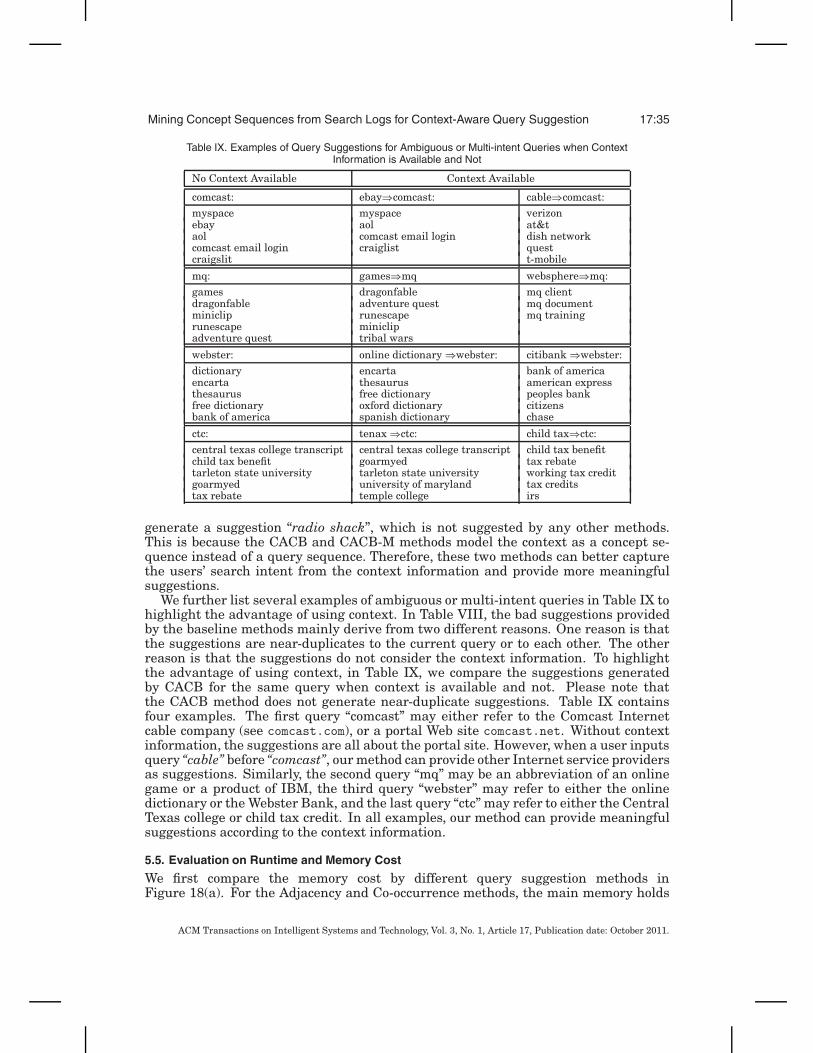
Mining Concept Sequences from Search Logs for Context-Aware Query Suggestion 17:35
Table IX. Examples of Query Suggestions for Ambiguous or Multi-intent Queries when ContextInformation is Available and Not
No Context Available Context Available
comcast: ebay⇒comcast: cable⇒comcast:myspace myspace verizonebay aol at&taol comcast email login dish networkcomcast email login craiglist questcraigslit t-mobile
mq: games⇒mq websphere⇒mq:games dragonfable mq clientdragonfable adventure quest mq documentminiclip runescape mq trainingrunescape miniclipadventure quest tribal wars
webster: online dictionary⇒webster: citibank⇒webster:dictionary encarta bank of americaencarta thesaurus american expressthesaurus free dictionary peoples bankfree dictionary oxford dictionary citizensbank of america spanish dictionary chase
ctc: tenax⇒ctc: child tax⇒ctc:central texas college transcript central texas college transcript child tax benefitchild tax benefit goarmyed tax rebatetarleton state university tarleton state university working tax creditgoarmyed university of maryland tax creditstax rebate temple college irs
generate a suggestion “radio shack”, which is not suggested by any other methods.This is because the CACB and CACB-M methods model the context as a concept se-quence instead of a query sequence. Therefore, these two methods can better capturethe users’ search intent from the context information and provide more meaningfulsuggestions.
We further list several examples of ambiguous or multi-intent queries in Table IX tohighlight the advantage of using context. In Table VIII, the bad suggestions providedby the baseline methods mainly derive from two different reasons. One reason is thatthe suggestions are near-duplicates to the current query or to each other. The otherreason is that the suggestions do not consider the context information. To highlightthe advantage of using context, in Table IX, we compare the suggestions generatedby CACB for the same query when context is available and not. Please note thatthe CACB method does not generate near-duplicate suggestions. Table IX containsfour examples. The first query “comcast” may either refer to the Comcast Internetcable company (see comcast.com), or a portal Web site comcast.net. Without contextinformation, the suggestions are all about the portal site. However, when a user inputsquery “cable” before “comcast”, our method can provide other Internet service providersas suggestions. Similarly, the second query “mq” may be an abbreviation of an onlinegame or a product of IBM, the third query “webster” may refer to either the onlinedictionary or the Webster Bank, and the last query “ctc” may refer to either the CentralTexas college or child tax credit. In all examples, our method can provide meaningfulsuggestions according to the context information.
5.5. Evaluation on Runtime and Memory Cost
We first compare the memory cost by different query suggestion methods inFigure 18(a). For the Adjacency and Co-occurrence methods, the main memory holds
ACM Transactions on Intelligent Systems and Technology, Vol. 3, No. 1, Article 17, Publication date: October 2011.

17:36 Z. Liao et al.
a lookup table where the key is a query and the value is the set of candidate querysuggestions for that query. Since the set of query pairs extracted from sessions by theCo-occurrence method is much larger than that by the Adjacency method, the memorycost by the Co-occurrence method is larger than that by the Adjacency method. Forthe N-gram method, the data structure to be held in the main memory is a query-sequence suffix tree, which is similar to a concept-sequence suffix tree as describedin Section 4.2. The only difference is that in a query-sequence suffix tree, each noderepresents a query instead of a concept. Since the N-gram method indexes not only ad-jacent query pairs but also query sequences with more than two queries, the memorycost of the N-gram method is larger than that of the Adjacency method. On the otherhand, the query sequences indexed by the N-gram method keep the original order ofqueries in sessions. Therefore, the memory cost of the N-gram method is still smallerthan that of the Co-occurrence method, where the indexed query pairs do not need tobe adjacent in the sessions. The CACB method is supported by a concept-sequencesuffix tree as well as a mapping table which maps a query to a concept. The size of theconcept-sequence suffix tree is smaller than that of the query-sequence suffix tree bythe N-gram method, since each concept node includes a set of similar queries. How-ever, the extra cost of the mapping table makes the total memory cost of the CACBmethod larger than that of the N-gram method. Please note that some concepts haveno following concepts in sessions and thus cannot be used for query suggestion. There-fore, those concepts are not indexed in the concept-sequence suffix tree and it is notnecessary to hold their mapping entries in the main memory. Finally, compared withthe CACB method, the CACB-M method needs additional memory to hold the termand URL feature vectors. Therefore, the memory cost of the CACB-M method is thelargest. Again, we only need to hold the feature vectors for those concepts indexedin the concept-sequence suffix tree. Although the CACB-M method costs the mostmemory, it requires less than 2G memory for the full dataset. Such a requirement isacceptable for a modern server.
We then compare the runtime for different methods. Basically, the runtime of all themethods include two parts. One is the offline mining time, and the other is the onlinequery suggestion time. The offline mining time for our method consists of two parts,that is, (a) the time for clustering the click-through bipartite to generate concepts, and(b) the time to mine frequent concept sequences from session data and construct theconcept sequence suffix tree. For all the baseline methods, since they do not generateconcepts, the offline mining time only includes (b’), which is the time to mine frequentquery pairs or sequences from session data and construct the query suggestion lookuptable or the query sequence suffix tree. Since we have reported the clustering time ofour method at different scales in Figure 13, in the following, we only compare (b) and(b’) of different methods.
Figure 18(b) shows the runtime of mining frequent patterns for all the methods ondifferent percentages of the full data. Recall that in Section 4.2 we develop a method todistributively mine frequent patterns under the map-reduce programming model. Inthis experiment, we mine the query pairs and sequences for all the baseline methods ina similar way. In Figure 18(b), the three baseline methods have different runtime be-cause they mine different frequent patterns. For example, given a session qs = q1q2q3,the Adjacency method generates two query pairs at the map step, that is, q1q2 andq2q3; the N-Gram method generates two subsequences q1q2 and q1q2q3; and the Co-occurrence method generates six query pairs, including q1q2, q1q3, q2q1, q2q3, q3q1,and q3q2. Since the Adjacency method only mines length-2 patterns and restricts thequeries should appear adjacent in sessions, the runtime is the shortest. The N-grammethod mines various length patterns. Thus, its runtime is longer than that of theAdjacency method. The Co-occurrence method does not constrain the order of queries
ACM Transactions on Intelligent Systems and Technology, Vol. 3, No. 1, Article 17, Publication date: October 2011.

Mining Concept Sequences from Search Logs for Context-Aware Query Suggestion 17:37
Fig. 18. (a) The memory cost of different query suggestion methods. (b) The runtime of mining and indexingcandidate suggestions.
and generates the largest number of patterns. Consequently, it needs more time thanthat by the Adjacency and the N-Gram methods. The CACB(-M) method needs theoverhead to convert a query sequence into a concept sequence before it mines frequentpatterns. From Figure 18(b), we can see such overhead makes it more costly than theAdjacency and the N-gram methods. When comparing CACB(-M) with Co-occurrence,we can see that the overhead of the former makes it more expensive than the latterwhen the dataset is small, that is, smaller than 30% of the full data. However, whenthe dataset grows larger, the runtime of CACB(-M) is smaller than that of the Co-occurrence method since CACB(-M) restricts the order of concepts and thus generatesa smaller number of frequent patterns.
Finally, we conduct a series of experiments to thoroughly evaluate the online querysuggestion time for all the methods. In the first experimental setting, we randomlypick up 10,000 single-query sessions as test cases and calculate the average time fordifferent methods to provide query suggestions. Therefore, in this setting, the N-grammethod have the same with the Adjacency method. Moreover, in this setting, we donot use the term and URL feature vectors to capture novel queries. In other words,the CACB method is the equivalent with the CACB-M method in this setting. AsFigure 19(a) shows, the Adjacency and the N-gram method has comparable perfor-mance, while the Co-occurrence method is slower. This is because the Co-occurrencemethod has to search a larger lookup table. The online response time of the CACB(-M) is the slowest, since it needs to map the input query into the correspondingconcept.
In the second experimental setting, we randomly pick up 10,000 sessions with atleast two queries as test cases. Again, we shut off the term and URL feature vectorsin this setting. As indicated by Figure 19(b), when context is available, both context-aware methods, that is, the N-Gram method and the CACB(-M) method, cost morethan those noncontext-aware methods. This is because the context-aware methodsneed to search deep in the suffix tree to match the context information.
In the last experimental setting, we randomly pick up 10,000 sessions where at leastone query in the session is not covered by the CACB method. Then we compare theruntime when the term and URL features are switched on and off. From Figure 19(c),we can see that using the term and URL features to cover novel queries is quite ex-pensive, which costs almost ten times the response time when the features are shutoff. However, even when the term and URL features are turned on to capture novelqueries, the total response time is still small, that is, about 0.3 millisecond. Suchresponse time is feasible for a commercial search engine, since the query suggestionprocess can be conducted in parallel with search results ranking.
ACM Transactions on Intelligent Systems and Technology, Vol. 3, No. 1, Article 17, Publication date: October 2011.

17:38 Z. Liao et al.
Fig. 19. The online runtime of different methods when: (a) context is not available and (b) context is avail-able. (c) The online runtime of CACB-M when the term and URL feature vectors are turned on and off. They-axis is in 10−6 seconds.
6. CONCLUSION
In this article, we proposed a novel approach to query suggestion using click-throughand session data. Unlike previous methods, our approach groups similar queries intoconcepts and models context information as sequences of concepts. The experimentalresults on a large-scale dataset containing billions of queries and URLs clearly showour approach outperforms three baselines in both coverage and quality.
In the future, we will extend our context-aware approach to other search applica-tions, such as query expansion, query substitution, query categorization, and docu-ment ranking. Moreover, we will explore a uniform framework which summarizescontext patterns and support various context-aware applications at the same time.
REFERENCESANAGNOSTOPOULOS, A., BECCHETTI, L., CASTILLO, C., AND GIONIS, A. 2010. An optimization framework
for query recommendation. In Proceedings of the 3rd ACM International Conference on Web Search andData Mining (WSDM’10). ACM, New York, 161–170.
BAEZA-YATES, R. AND TIBERIM A. 2007. Extracting semantic relations from query logs. In Proceedings ofthe 13th ACM SIGKDD International Conference on Knowledge Discovery and Data Mining (KDD’07).ACM, 76–85.
BAEZA-YATES, R. A., HURTADO, C. A., AND MENDOZA, M. 2004. Query recommendation using querylogs in search engines. In Proceedings of the EDBT Workshop on Clustering Information over the Web.Springer, 588–596.
BEEFERMAN, D. AND BERGER, A. 2000. Agglomerative clustering of a search engine query log. In Pro-ceedings of the 6th ACM SIGKDD International Conference on Knowledge Discovery and Data Mining(KDD’00). ACM, 407–416.
BEN-DOR, A., SHAMIR, R., AND YAKHINI, Z. 1999. Clustering gene expression patterns. J. Comput.Biol. 6, 3/4, 281–297.
BOLDI, P., BONCHI, F., CASTILLO, C., DONATO, D., AND VIGNA, S. 2009. Query suggestions using query-flow graphs. In Proceedings of the Workshop on Web Search Click Data (WSCD’09). ACM, 56–63.
BOLDI, P., BONCHI, F., CASTILLO, C., DONATO, D., GIONIS, A., AND VIGNA, S. 2008. The query-flowgraph: model and applications. In Proceedings of the 17th ACM Conference on Information and Knowl-edge Management (CIKM’08). 609–618.
CAO, G., NIE, J.-Y., GAO, J., AND ROBERTSON, S. 2008. Selecting good expansion terms for pseudo-relevance feedback. In Proceedings of the 17th ACM Conference on Information and Knowledge Man-agement (SIGIR’08). ACM, 243–250.
CAO, H., JIANG, D., PEI, J., HE, Q., LIAO, Z., CHEN, E., AND LI, H. 2008. Context-Aware query sugges-tion by mining click-through and session data. In Proceedings of the 14th ACM SIGKDD InternationalConference on Knowledge Discovery and Data Mining (KDD’08). ACM, 875–883.
CHIRITA, P. A., FIRAN, C. S., AND NEJDL, W. 2007. Personalized query expansion for the web. In Pro-ceedings of the 30th Annual International ACM SIGIR Conference on Research and Development inInformation Rtrieval (SIGIR’07). 7–14.
ACM Transactions on Intelligent Systems and Technology, Vol. 3, No. 1, Article 17, Publication date: October 2011.

Mining Concept Sequences from Search Logs for Context-Aware Query Suggestion 17:39
CRASELL, N. AND SZUMMER, M. 2007. Random walks on the click graph. In Proceedings of the 30thAnnual International ACM SIGIR Conference on Research and Development in Information Retrieval(SIGIR’07). 239–246.
CUI, H., WEN, J., NIE, J., AND MA, W. 2002. Probabilistic query expansion using query logs. In Proceedingsof the 11th International Conference on World Wide Web (WWW’02). 325–332.
DEAN, J. AND GHEMAWAT, S. 2004. MapReduce: simplified data processing on large clusters. In Proceedingsof the 6th Symposium on Operating System Design and Implementation (OSDI’04). 137–150.
ESTER, M., KRIEGEL, H., SANDER, J., AND XU, X. 1996. A density-based algorithm for discovering clustersin large spatial databases with noise. In Proceedings of the 2nd International Conference on KDD.226–231.
FONSECA, B. M., GOLGHER, P., POSSAS, B., RIBEIRO-NETO, B., AND ZIVIANI, N. 2005. Concept-Basedinteractive query expansion. In Proceedings of the 14th ACM International Conference on Informationand Knowledge Management (CIKM’05). 696–703.
GAO, J., YUAN, W., LI, X., DENG, K., AND NIE, J.-Y. 2009. Smoothing clickthrough data for web searchranking. In Proceedings of the 32nd Annual International ACM SIGIR Conference on Research andDevelopment in Information Retrieval (SIGIR’09). 355–362.
GUO, J., XU, G. AND LI, H., AND CHENG, X. 2008. A unified and discriminative model for query refinement.In Proceedings of the 31st Annual International ACM SIGIR Conference on Research and Developmentin Information Retrieval (SIGIR’08). 379–386.
HINNEBURG A. AND KEIM, D. A. 1999. Optimal grid-clustering: Towards breaking the curse of dimension-ality in high-dimensional clustering. In Proceedings of the 25th International Conference on Very LargeData Bases (VLDB’99). 506–517.
HUANG, C., CHIEN, L., AND OYANG, Y. 2003. Relevant term suggestion in interactive web search based oncontextual information in query session logs. J. Amer. Soc. Inf. Sci. Technol. 54, 7, 638–649.
JANSEN, B.J., SPINK, A., BATEMAN, J., AND SARACEVIC, T. 1998. Real life information retrieval: A studyof user queries on the web. SIGIR Forum, 5–17.
JENSEN, E. C., BEITZEL, S., CHOWDHURY, A., AND FRIDER, O. . 2006. Query phrase suggestion fromtopically tagged session logs. In Proceedings of the 7th International Conference on Flexible QueryAnswering Systems (FQAS’06). 185–196.
JONES, R., REY, B. MADANI, O. AND GREINER, W. 2006. Generating query substitutions. In Proceedingsof the 15th International Conference on World Wide Web (WWW’06). 387–396.
KRAFT, R. AND ZIEN, J. 2004. Mining anchor text for query refinement. In Proceedings of the 13thInternational Conference on World Wide Web (WWW’04). 666–674.
LAU, T. AND HORVITZ, E. 1999. Patterns of search: Analyzing and modeling web query refinement. InProceedings of the 7th International Conference on User Modeling. 119–128.
LAVRENKO, V. AND CROFT, W.B. 2001. Relevance based language models. In Proceedings of the 24thAnnual International ACM SIGIR Conference on Research and Development in Information Retrieval(SIGIR’01). 120–127.
LIU, S., LIU, F., YU, C., AND MENG, W. 2004. An effective approach to document retrieval via utilizingwordnet and recognizing phrases. In Proceedings of the 27th Annual International ACM SIGIRConference on Research and Development in Information Retrieval (SIGIR’04). ACM, 266–272.
MAGENNIS, M. AND VAN RIJSBERGEN, C.J. 1997. The potential and actual effectiveness of interactivequery expansion. In Proceedings of the 20th Annual International ACM SIGIR Conference on Researchand Development in Information Retrieval (SIGIR’97). 324–332.
MEI, Q., KLINKNER, K., KUMAR, R., AND TOMKINS, A. 2009. An analysis framework for search sequences.In Proceedings of the 18th ACM Conference on Information and Knowledge Management (CIKM’09).1991–1996.
MEI, Q., ZHOU, D., AND CHURCH, K. 2008. Query suggestion using hitting time. In Proceedings of the 17thACM Conference on Information and Knowledge Management (CIKM’08). 469–478.
METZLER, D. AND CROFT, W.B. 2007. Latent concept expansion using markov random fields. In InProceedings of the 30th Annual International ACM SIGIR Conference on Research and Development inInformation Retrieval (SIGIR’07). 311–318.
PEI, J., HAN, J., MORTAZAVI-ASL, B., PINTO, H., CHEN, Q., DAYAL, U., AND HSU, M.-C. 2001. PrefixS-pan: Mining sequential patterns efficiently by prefix-projected pattern growth. In Proceedings of theInternational Conference on Data Engineering (ICDE’01). 215–224.
RIEH, S. Y. AND XIE, H. 2001. Patterns and sequences of multiple query reformulations in web searching:A preliminary study. In Proceedings of ASIS&T Annual Meeting. 246–255.
ACM Transactions on Intelligent Systems and Technology, Vol. 3, No. 1, Article 17, Publication date: October 2011.

17:40 Z. Liao et al.
ROUSSEEUW, P. 1987. Silhouettes: a graphical aid to the interpretation and validation of cluster analysis.J. Comput. Appl. Math. 20, 53–65.
SADIKOV, E., MADHAVAN, J., WANG, L., AND HALEVY, A. 2010. Clustering query refinements by userintent. In Proceedings of the International World Wide Web Conference (WWW’10). 841–850.
SAHAMI, M. AND HEILMAN, T.D. 2006. A web-based kernel function for measuring the similarity of shorttext snippets. In Proceedings of the 15th International Conference on World Wide Web (WWW’06).377–386.
SILVERSTEIN, C., MARAIS, H., HENZINGER, M., AND MORICZ, M. 1999. Analysis of a very large websearch engine query log. ACM SIGIR Forum, 6–12.
SRIKANT, R. AND AGRAWAL, R. 1996. Mining sequential patterns: Generalizations and performanceimprovements. In Proceedings of the 5th International Conference of Extending Database Technology(EDBT’96). 3–17.
TAN, P. N., STEINBACH, M., AND KUMAR, V. 2005. Introduction to Data Mining, 1st Ed. Addison-WesleyLongman Publishing Co., Inc.
TERRA, E. AND CLARKEM, C.L.A. 2004. Scoring missing terms in information retrieval tasks. In Proceed-ings of the 13th ACM International Conference on Information and Knowledge Management (CIKM’04).50–58.
WEN, J., NIE, J., AND ZHANG, H. 2001. Clustering user queries of a search engine. In Proceedings of the10th International Conference on World Wide Web (WWW’01). 162–168.
WHITE, R. W., BAILEY, P., AND CHEN, L. 2009. Predicting user interests from contextual information.In Proceedings of the 32nd International ACM SIGIR Conference on Research and Development inInformation Retrieval (SIGIR’09). 363–370.
WHITE, R. W., BENNETT, P.N., AND DUMAIS, S.T. 2010. Predicting short-term interests using activity-based search context. In Proceedings of 19th International Conference on Information and KnowledgeManagement (CIKM’10). 1009–1018.
WHITE, R. W., BILENKO, M., AND CUCERZAN, S. 2007. Studying the use of popular destinations to enhanceweb search interaction. In Proceedings of the 30th Annual International ACM SIGIR Conference onResearch and Development in Information Retrieval (SIGIR’07). 159–166.
ZHANG, T., RAMAKRISHNAN, R., AND LIVNY, M. 1996. BIRCH: An efficient data clustering method forvery large databases. In Proceedings of the ACM SIGMOD International Conference on Management ofData. 103–114.
Received October 2010; revised February 2011; accepted April 2011
ACM Transactions on Intelligent Systems and Technology, Vol. 3, No. 1, Article 17, Publication date: October 2011.


![Learning from Macro-expression: a Micro-expression ...staff.ustc.edu.cn/~cheneh/paper_pdf/2020/Bin-Xia-MM.pdfframework CapsuleNet [30] to recognize micro-expressions. Peng et al. [28]](https://img.dokumen.tips/doc/110x75/60df6c9ae8c43e0e553f9272/learning-from-macro-expression-a-micro-expression-staffustceducnchenehpaperpdf2020bin-xia-mmpdf.jpg)