Geoinformatica (2006) 10: 239–260DOI 10.1007/s10707-006-9827-8

Mining Co-Location Patterns with Rare Eventsfrom Spatial Data Sets

Yan Huang · Jian Pei · Hui Xiong

© Springer Science + Business Media, LLC 2006

Abstract A co-location pattern is a group of spatial features/events that are fre-quently co-located in the same region. For example, human cases of West Nile Virusoften occur in regions with poor mosquito control and the presence of birds. For co-location pattern mining, previous studies often emphasize the equal participationof every spatial feature. As a result, interesting patterns involving events withsubstantially different frequency cannot be captured. In this paper, we address theproblem of mining co-location patterns with rare spatial features. Specifically, we firstpropose a new measure called the maximal participation ratio (maxPR) and showthat a co-location pattern with a relatively high maxPR value corresponds to a co-location pattern containing rare spatial events. Furthermore, we identify a weakmonotonicity property of the maxPR measure. This property can help to developan efficient algorithm to mine patterns with high maxPR values. As demonstrated

A preliminary version of the paper appeared as [13].

The research of the second author is supported in part by Natural Sciences and EngineeringResearch Council of Canada under grant number 312194-05 and National Science Foundationof the United States under grant number IIS-0308001. All opinions, findings, conclusions andrecommendations in this paper are those of the authors and do not necessarily reflect the viewsof the funding agency.

Y. Huang (B)Department of Computer Science and Engineering, University of North Texas, Texas, USAe-mail: huangyan@unt.edu

J. PeiSchool of Computing Science, Simon Fraser University, Burnaby, Canadae-mail: jpei@cs.sfu.ca

H. XiongManagement Science and Information Systems Department, Rutgers University, Newark, USAe-mail: hui@rbs.rutgers.edu

240 Geoinformatica (2006) 10: 239–260

by our experiments, our approach is effective in identifying co-location patterns withrare events, and is efficient and scalable for large-scale data sets.

Keywords Spatial data mining · Co-location patterns · Spatial association rules

1 Introduction

Advanced spatial data collecting systems, such as NASA Earth’s Observing System(EOS) and Global Positioning System (GPS), have been accumulating increasinglylarge spatial data sets [8], [12], [18], [24], [25], [30]. For instance, since 1999, morethan a terabyte of data has been produced by EOS every day. These spatial datasets with explosive growth rate are considered nuggets of valuable information.The automatic discovery of interesting, potentially useful, and previously unknownpatterns from large spatial datasets is being widely investigated via various spatialdata mining [16], [23], [24], [29] techniques. Classical spatial pattern mining methodsinclude spatial clustering [22], spatial characterization [9], spatial outlier detection[27], spatial prediction [28], and spatial boundary shape matching [15].

Mining spatial co-location patterns [7], [10], [11], [20], [21], [26], [31] is an impor-tant spatial data mining task. A spatial co-location pattern is a set of spatial featuresthat are frequently located together in spatial proximity. To illustrate the idea of spatialco-location patterns, let us consider a sample spatial data set, as shown in Fig. 1. Inthe figure, there are various spatial instances with different spatial features that aredenoted by different symbols. As can be seen, spatial feature + and × tend to belocated together because their instances are frequently located in spatial proximity.

The problem of mining spatial co-location patterns can be related to variousapplication domains. For example, in location based services, different services arerequested by service subscribers from their mobile PDA’s equipped with locating de-vices such as GPS. Some types of services may be requested in proximate geographicarea, such as finding the nearest Italian restaurant and the nearest parking place.Location based service providers are very interested in finding what services arerequested frequently together and located in spatial proximity. This information canhelp them improve the effectiveness of their location based recommendation systemswhere a user requested a service in a location will be recommended a service in anearby location. Knowing co-location patterns in location based services may alsoenable the use of pre-fetching to speed up service delivery. In ecology, scientists areinterested in finding frequent co-occurrences among spatial features, such as drought,EI Nino, substantial increase/drop in vegetation, and extremely high precipitation.

The previous studies on co-location pattern mining emphasize frequent co-occurrences of all the features involved. This marks off some valuable patternsinvolving rare spatial features. We say a spatial feature is rare if its instances aresubstantially less than those of the other features in a co-location. This definition of“rareness” is relative with respect to other features in a co-location. A feature couldbe rare in one co-location but not rare in another. For example, if the spatial featureA has 10 instances, the spatial feature B has 20 instances, and the spatial feature Chas 10,000 instances. A is not considered a rare feature in the co-location {A, B} butit is considered a rare feature in co-location {A, C}. Of course, a feature with verysmall number of instances are often rare in many co-location patterns.

Geoinformatica (2006) 10: 239–260 241

Fig. 1 An illustration of spatial co-location patterns. Shapes represent different spatial feature types.Instances of spatial features in sets {‘+’, ‘×’} and {‘o’, ‘*’} tend to be located together

In many cases, it is important to capture co-location patterns with rare features.For example, it is believed that human West Nile Virus disease [2] often occursin regions with poor mosquito control and the presence of birds. The Center forDisease Control has received confirmation from state agencies of 8,219 human casesof West Nile Virus for the year 2003. However, due to numerous locations with poormosquito control and the presence of birds, we may not find that poor mosquitocontrol and domestic animals are strongly co-located with human West Nile Virusdisease using the existing co-location mining methods.

As another example, in a case settled in 1996 [1], PG&E’s nearby plant wasleaching chromium 6, a rust inhibitor, into the water supply of Hinkley California,and the suit blamed the chemical for dozens of symptoms, ranging from nosebleedsto breast cancer, Hodgkin’s disease, miscarriages and spinal deterioration. Theprosecutors argued that chromium 6 contaminated water caused nosebleeds, breastcancer, etc. in their nearby region with high probability. Again, this is a typical co-location pattern involving rare spatial features; that is, the spatial event “chromium6 contaminated water” is rare compared to nose-bleeding.

242 Geoinformatica (2006) 10: 239–260

Therefore, it is necessary to explore new methods to discover co-location patternswith rare spatial features, which is the motivation of this paper. However, the existingco-location mining algorithms [20], [26] have difficulties in identifying such patterns.In general, the challenges of mining spatial co-location patterns with rare spatialfeatures lay in two aspects.

1. How to identify and measure spatial co-location patterns involving rare spatialfeatures ?Strong interactions involving rare spatial features are often marked off in pre-vious methods, since they require frequent co-occurrences of all features in theco-location patterns. Many measures are based on the measures of frequency orminimum participation ratio where rare events are unfavorable.Our contributions. In this paper, we propose a novel measure called maximalparticipation ratio, which can incorporate the spatial co-location patterns in thepresence of rare spatial features. We show that finding spatial co-locations fromspatial data sets with rare spatial features can be achieved by finding co-locationpatterns with respect to the maximal participation index.

2. How to mine the patterns involving rare spatial features efficiently?Even though we have a good measure for co-location patterns in the presenceof rare spatial features, it is still challenging to find all the patterns efficiently.One dominant obstacle is that the maximal participation ratio is not monotonicwith respect to co-location pattern containment relation. Thus, the conventionalapriori-like pruning technique [4] cannot be applied. Without proper pruning,there could be many possible combinations. Checking them one by one may becomputationally prohibitive in many cases.Our contributions. In this paper, we study the problem of efficiently miningco-location patterns with rare spatial features systematically. We propose twoalgorithms. The first algorithm is a rudimentary extension of the apriori-like [4]solution. It uses a very low participation index threshold to prune and use themaximal participation ratio threshold to do a post-processing. It is not efficientsince it has to enumerate many patterns.Our second algorithm is much more efficient. It exploits an interesting weakmonotonic property of the maximal participation ratio to push the maximalparticipation ratio threshold deep into the mining. It achieves good performancein most cases.We conduct an extensive performance study to test our methods. The experimen-tal results show that our methods are effective, efficient and scalable for mininglarge spatial databases.

The remainder of this paper is organized as follows. In Section 2, we review relatedwork. We recall important concepts of association rule mining and compare it withspatial co-location mining in Section 3. Section 4 presents an overview of the co-location pattern mining framework [26]. In Section 5, we introduce the maximalparticipation ratio. Efficient algorithms for mining co-location patterns with rarefeatures are proposed in Section 6. An extensive performance study is reported inSection 7. Finally, in Section 8, we draw conclusions and suggest future work.

Geoinformatica (2006) 10: 239–260 243

2 Related Work

The previous methods of mining co-location patterns can be divided into twocategories, namely the spatial data mining methods and the spatial statistics methods.They are reviewed briefly in this section.

2.1 Spatial Data Mining Methods

In [26], [31], efficient algorithms were proposed to mine spatial co-location patternsfrom spatial databases. A set of spatial features form a pattern if, for each spatialfeature, at least s% instances of that feature form a clique with some instance of allthe rest features in the pattern for a given neighborhood relationship, such as anEuclidean distance threshold. The parameter s% is called the participation index. Inother words, a set of spatial features form a pattern if whenever a feature of the setis observed, with a probability of at least s%, all other features are also observed inspatial proximity. When the number of objects of different spatial features spans awide range, the popular features (features with a large number of objects) tend to geta low ratio compared to rare features (features with a small number of instances).In [31], spatial co-location patterns were generalized and expressed by multi-wayspatial joins. The space partitioning algorithms were proposed to solve the spatialco-location pattern mining problem. The proposed algorithm is not restricted to aparticular interesting measure.

In [20], graphs formed by neighboring spatial instances are partitioned to disjointparts. A frequency-based pruning technique is developed. This frequency-basedpruning method also favors popular spatial features. A clustering-based map overlayapproach [10], [11] treats every spatial attribute as a map layer and considers spatialclusters (regions) of point-data in each layer as candidates for mining associations.Given X and Y as sets of layers, a clustered spatial association rule is defined asX ⇒ Y(CS%, CC%), for X

⋂Y = ∅, where CS% is the clustered support, defined as

the ratio of the area of the cluster (region) that satisfies both X and Y to the totalarea of the region S under investigation, and CC% is the clustered confidence, whichcan be interpreted as CC% of the areas of clusters (regions) of X intersect with areasof clusters(regions) of Y. However, instances of rare spatial features, e.g., chromium6 populated water sources, do not always form clusters or regions.

The reference feature centric model proposed in [17] enumerates proximityneighborhoods to “materialize” a set of transactions around instances of a userspecified reference spatial feature. Transactions are created around instances of oneuser-specified spatial feature. The association rules are derived using the apriorialgorithm [4]. The rules found are all related to the reference feature. The supportbased apriori pruning marks off co-location patterns with rare spatial features.

Munro et al. [21] described the need for mining complex relationships in spatialdata including multi-feature colocation, self-colocation, one-to-many relationships,self-exclusion and multi-feature exclusion.

2.2 Spatial Statistics Methods

In spatial statistics, some dedicated techniques such as cross k-functions with MonteCarlo simulations [7], mean nearest-neighbor distance, and spatial regression models

244 Geoinformatica (2006) 10: 239–260

[6] have been developed to test the co-location of two spatial features and findpairs of co-located spatial features. However, the Monte Carlo simulation couldbe expensive. Another approach is to arbitrarily partition the space into a lattice.For each cell of the lattice, count the number of instances of each spatial feature.Pairwise correlation of spatial features could be found by tests such as χ2 [7] orusing classic association rule mining algorithms such as apriori [4] by treating eachcell as a transaction. Arbitrary partitioning may loss neighboring instances acrossborders of cells. Both the cross k-function and the pair wise correlation cannot beeasily extended to the cases with more than two spatial features.

To the best of our knowledge, this is the first systematic study on mining co-location patterns with rare features in the spatial context.

3 Association Rule Mining

Since spatial co-location pattern mining resembles association pattern mining [3] inmany aspects, we review the basic concepts of association rules in this section.

Since its introduction [3], the problem of mining association rules from largedatabases has been the subject of numerous studies. The association rule miningproblem is defined as follows.

Let I = {i1, i2, . . . , im} be a set of m items. Let T D = {T1, T2, . . . , Tn} be atransactional database where Ti(i ∈ [1, n]) is a transaction which is a subset of itemsin I . For an itemset Y ⊆ I , the support of Y is the number of transactions containingY in T D, i.e., sup(Y) = |{Ti|Ti ⊇ Y}|. Y is of size k if |Y| = k.

The confidence of an association rule in the form of X → Y, where X ∩ Y = ∅, isthe ratio of the support of X ∪ Y versus the support of X. Itemset Y is a frequentpattern if the support of Y is no less than a minimum support threshold specifiedby user. We compare and contrast frequent pattern mining and spatial co-locationmining in Table 1.

The support of itemsets has a downward closure property (sometimes called theapriori property): the support of Y is no less than the support of any superset of Y.Because of the downward closure property of the support, a generate-and-test miningparadigm was employed by the apriori algorithm proposed in [4]. This approachgenerates candidates of size (k + 1) items set based on the size k frequent itemsets.The set of size (k + 1) candidates includes all and only those itemsets of size (k + 1)

whose size k subsets are all frequent. False candidates are pruned by scanning thetransactions before the next iteration.

Table 1 Comparison offrequent pattern mining andspatial co-location mining

Frequent pattern mining Co-Location mining

Item Spatial featureItem set Spatial feature setFrequent pattern Co-location patternSupport Spatial interestingness measuresTransactional database Spatial database

Geoinformatica (2006) 10: 239–260 245

4 Co-Location Patterns in Spatial Databases

In this section, we review a framework of mining co-location patterns, since ourproposed solution in this paper is based on this model. The framework was proposedin [26] and is based on the participation index. We will point out why such aframework still may miss some co-location patterns involving rare spatial features.In the next section, we will extend the framework to mine co-location patterns withrare spatial features.

For a spatial data set S, let F = { f1, . . . , fk} be a set of boolean spatial features.Let i = {i1, . . . , in} be a set of n instances in S, where each instance is a vector〈instance-id, location, spatial features〉. The spatial feature f of instance i is denotedby i. f . We assume that the spatial features of an instance are from F and the locationis within the spatial framework of the spatial database. Furthermore, we assume thatthere exists a neighborhood relation R over pairwise instances in S.

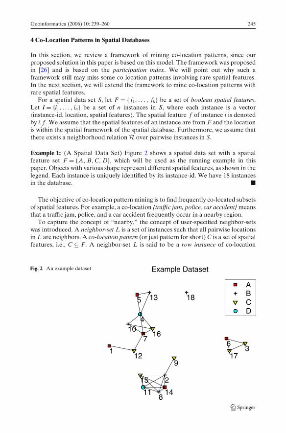
Example 1: (A Spatial Data Set) Figure 2 shows a spatial data set with a spatialfeature set F = {A, B, C, D}, which will be used as the running example in thispaper. Objects with various shape represent different spatial features, as shown in thelegend. Each instance is uniquely identified by its instance-id. We have 18 instancesin the database. �

The objective of co-location pattern mining is to find frequently co-located subsetsof spatial features. For example, a co-location {traffic jam, police, car accident} meansthat a traffic jam, police, and a car accident frequently occur in a nearby region.

To capture the concept of “nearby,” the concept of user-specified neighbor-setswas introduced. A neighbor-set L is a set of instances such that all pairwise locationsin L are neighbors. A co-location pattern (or just pattern for short) C is a set of spatialfeatures, i.e., C ⊆ F. A neighbor-set L is said to be a row instance of co-location

Fig. 2 An example dataset

246 Geoinformatica (2006) 10: 239–260

pattern C if every feature in C appears as a feature of an instance in L, and thereexists no proper subset of L does so. We denote all row instances of a co-locationpattern C by rowset(C).

Example 2: (Neighbor-set, row instance and rowset) In Fig. 2, the neighborhoodrelation R is defined based on Euclidean distance. Two instances are neighbors iftheir Euclidean distance is less than a user specified threshold. Neighboring instancesare connected by edges. For instance, {3, 6, 17}, {4, 5, 13}, and {4, 7, 10, 16} are allneighbor-sets because each set forms a clique. Here, we use the instance-id to referto an object in Fig. 2. Additional neighbor-sets include {6, 17}, {3, 6}, {2, 15, 11, 14},and {2, 15, 8, 11, 14}.

{A, B, C, D} is a co-location pattern. The neighborhood-set {14, 2, 15, 11} is arow instance of the pattern {A, B, C, D} but the neighborhood-set {14, 2, 8, 15, 11}is not a row instance of co-location {A, B, C, D} because it has a proper subset{14, 2, 15, 11} which contains all the features in {A, B, C, D}.

Finally, the rowset({A, B, C, D})= {{7, 10, 16, 4}, {14, 2, 15, 11},{14, 8, 15, 11}}. �

For a co-location rule R : A → B, the conditional probability cp(R) of R isdefined as

|{L ∈ rowset(A)|∃L′ s.t. (L ⊆ L′) ∧ (L′ ∈ rowset(A ∪ B))}||rowset(A)|

In words, the conditional probability is the probability that a neighbor-set inrowset(A) is part of a neighbor-set in rowset(A ∪ B). Intuitively, the conditionalprobability p indicates that, whenever we observe the occurrences of spatial featuresin A, the probability to find occurrence of B in a nearby region is p.

Example 3: (Conditional probability) In Fig. 2, based on the Euclidean distancerelation R as described in Example 2,

rowset({A, B, C, D}) = {{7, 10, 16, 4}, {14, 2, 15, 11}, {14, 8, 15, 11}},and

rowset({A, B}) = {{7, 10}, {14, 2}, {5, 13}, {14, 8}}.Since |rowset({A, B})| = 4, only 3 rows of {A, B} satisfy the subset condition, i.e.,row {7, 10} of {A, B} is a subset of row {7, 10, 16, 4} of {A, B, C, D}, row {14, 2} of{A, B} is a subset of row {14, 2, 15, 11} of {A, B, C, D} and row {14, 8} of {A, B} is asubset of row {14, 8, 15, 11} of {A, B, C, D}, the conditional probability cp({A, B} →{C, D}) = 3

4 = 75%. �

Given a spatial database S, to measure how a spatial feature f is co-located withother features in co-location pattern C, a participation ratio pr(C, f ) can be definedas

pr(C, f ) = |{r|(r ∈ S) ∧ (r. f = f ) ∧ (r is in a row instance of C)}|{r|(r ∈ S) ∧ (r. f = f )}|

Geoinformatica (2006) 10: 239–260 247

In words, a feature f has a partition ratio pr(C, f ) in pattern C means whereverthe feature f is observed, with probability pr(C, f ), all other features in C are alsoobserved in a neighbor-set.

In [26], a participation index was proposed to measure how all the spatial featuresin a co-location pattern are co-located. For a co-location pattern C, the participationindex PI(C) = min f∈C{pr(C, f )}. In words, wherever any feature in C is observed,with a probability of at least PI(C), all other features in C can be observed in aneighbor-set. A high participation index value indicates that the spatial features ina co-location pattern likely occur together. The participation index was proposedbecause in spatial application domain there are no natural “transactions” and thus“support” is not well-defined.

Given a user-specified participation index threshold min_prev, a co-location pat-tern is called prevalent if PI(C) ≥ min_ prev.

Example 4: (Participation ratio and participation index) To find the participationindex PI({A, B, C, D}) of pattern {A, B, C, D}, we first identify the rowsets of{A, B, C, D} as shown in Example 2, i.e., {{7, 10, 16, 4}, {14, 2, 15, 11}, {14, 8, 15, 11}}.

Among all the five instances of A, two of them, namely 7 and 14, haveB, C and D in a neighbor-set. So the participation ratio pr({A, B, C, D}, A) = 2

5 .Similarly, we can have pr({A, B, C, D}, B) = 3

5 , pr({A, B, C, D}, C) = 26 = 1

3 , andpr({A, B, C, D}, D) = 2

2 = 1. Taking the minimal of all the ratios, the participationindex PI({A, B, C, D}) of co-location {A, B, C, D} is 1

3 . �

As shown below, both the participation ratio and the participation index aremonotonic with respect to the size of co-location patterns.

Lemma 1: (Monotonicity of participation ratio and participation index [26]) Let Cand C′ be two co-location patterns such that C ⊂ C′. Then, for each feature f ∈ C,pr(C, f ) ≥ pr(C′, f ). Furthermore, PI(C) ≥ PI(C′).

Proof: To have the first claim in the lemma, we only need to show that for a spatialfeature f ∈ C,

|{r|(r ∈ S) ∧ (r. f = f ) ∧ (r is in a row instance of C)}| ≥|{r|(r ∈ S) ∧ (r. f = f ) ∧ (r is in a row instance of C′)}|

Since C ⊂ C′, every row instance of C′ contains a subset of instances which is arow instance of C. Thus, the inequality holds.

The second claim follows the fact that PI(C) = min f∈C{pr(C, f )} ≥min f∈C{pr(C′, f )} ≥ min f∈C′ {pr(C′, f )} = PI(C′). �

Based on Lemma 1, a level-by-level, iterative apriori-like algorithm was developedin [26] to find the complete set of prevalent patterns from a spatial database. Fordetails of the algorithm, please refer to [26].

It is interesting to note that, in the above prevalent co-location pattern miningframework, some co-location patterns involving rare spatial features may be unfor-tunately missed.

248 Geoinformatica (2006) 10: 239–260

Example 5: (A Co-location Pattern for West Nile Disease) Let us consider the co-location pattern C = {West Nile, poor mosquito control, domestic animal}. Supposeparticipation ratios

pr(C, West Nile ) = 85%,

pr(C, poor mosquito control) = 10%

and

pr(C, domestic animal) = 1%.

Then, PI(C) = min{85%, 10%, 1%} = 1%. As can be seen, even though West Nile isstrongly co-located with poor mosquito control and domestic animal, unfortunately,the whole co-location pattern is weak in the term of participation index because theWest Nile is rare compared to poor mosquito control and domestic animals. �

Can we extend the framework to mine such patterns even though their participationindex values are low? In other words, can we mine co-location patterns with rarespatial features? We will address this issue in the next two sections.

5 Maximal Participation Ratio

There is one important observation about co-location patterns with rare spatialfeatures, “even though the participation index of the whole pattern could be low,there must be some spatial feature(s) with high participation ratio(s) .” In Example 5,in pattern P = {West Nile, poor mosquito control, domestic animal}, the participa-tion index is low, since West Nile disease are rare compared to poor mosquito controland domestic animals. However, the participation ratio of “West Nile Virus” in thepattern is high.

The above observation motivates our extension of the participation index frame-work. For a co-location pattern C, we define the maximal participation ratio asmaxPR= max f∈C{pr(C, f )}. In words, a high maximal participation ratio value in-dicates that there are some spatial features strongly imply the pattern.

In general, given a co-location pattern C = { f1, . . . , fk}, we sort all spatial featuresin C in the participation ratio descending order. Without loss of generality, for agiven minimum maximal participation ratio threshold min_maxPR, suppose for i ∈[1, l] pr(C, fi) ≥ min_maxPR, where 1 ≤ i ≤ l ≤ k and l is the last spatial feature thathas participation ratio above the user given threshold. The output of the co-locationmining with rare spatial features will be in the form of 〈C = { f1, . . . , fk}, l〉. Then,we can say that if a spatial feature fi (1 ≤ i ≤ l) is observed in some location, then theprobability of observing all other spatial features in C − { fi} in a neighbor-set is at leastmaxPR(C).

Given a minimum maxPR threshold min_maxPR, the problem of mining co-location patterns with rare spatial features in a spatial database is to find the completeset of co-location patterns C such that maxPR(C) ≥ min_maxPR.

In general, every pattern that is significant in participation index is also significantin maximal participation ratio. In other words, mining co-location patterns with rare

Geoinformatica (2006) 10: 239–260 249

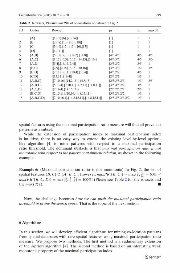
Table 2 Rowsets, PIs and maxPRs of co-locations of dataset in Fig. 2

ID Co-loc Rowset pr PI max PI

1 {A} {{1},{5},{6},{7},{14}} {1} 1 12 {B} {{2},{8},{10}, {13},{18}} {1} 1 13 {C} {{3},{9},{12}, {15},{16},{17}} {1} 1 14 {D} {{4},{11}} {1} 1 15 {A,B} {{5,13},{7,10},{14,2},{14,8}} {4/5,4/5} 4/5 4/56 {A,C} {{1,12},{6,3},{6,17},{14,15},{7,16}} {4/5,5/6} 4/5 5/67 {A,D} {{5,4},{14,1},{7,4}} {3/5,2/2} 3/5 18 {B,C} {{2,9},{2,15},{8,15},{10,16}} {3/5,3/6} 1/2 3/59 {B,D} {{2,11},{8,11},{10,4},{13,4}} {4/5,2/2} 4/5 110 {C,D} {{15,11},{16,4}} {2/6,2/2} 1/3 111 {A,B,C} {{7,10,16},{14,2,15},{14,8,15}} {2/5,3/5,2/6} 1/3 3/512 {A,B,D} {{5,13,4},{7,10,4},{14,2,11},{14,8,11}} {3/5,4/5,2/2} 3/5 113 {A,C,D} {{7,16,4},{14,15,11}} {2/5,2/6,2/2} 2/5 114 {B,C,D} {{2,15,11},{10,16,4},{8,15,11}} {3/5,2/6,2/2} 1/3 115 {A,B,C,D} {{7,10,16,4},{14,2,15,11},{14,8,15,11}} {2/5,3/5,2/6,2/2} 1/3 1

spatial features using the maximal participation ratio measure will find all prevalentpatterns as a subset.

While the extension of participation index to maximal participation indexis intuitive, there is no easy way to extend the existing level-by-level apriori-like algorithm [4] to mine patterns with respect to a maximal participationratio threshold. The dominant obstacle is that maximal participation ratio is notmonotonic with respect to the pattern containment relation, as shown in the followingexample.

Example 6: (Maximal participation ratio is not monotonic) In Fig. 2, the set ofspatial features {B, C} ⊂ {A, B, C}. However, maxPR({B, C}) = max{ 3

5 , 36 } = 60% ≤

maxPR({B, C, D}) = max{ 35 , 2

6 , 22 } = 100%! (Please see Table 2 for the rowsets and

the maxPR’s). �

Now, the challenge becomes how we can push the maximal participation ratiothreshold to prune the search space. That is the topic of the next section.

6 Algorithms

In this section, we will develop efficient algorithms for mining co-location patternsfrom spatial databases with rare spatial features using maximal participation ratiomeasure. We propose two methods. The first method is a rudimentary extensionof the Apriori algorithm [4]. The second method is based on an interesting weakmonotonic property of the maximal participation index.

250 Geoinformatica (2006) 10: 239–260

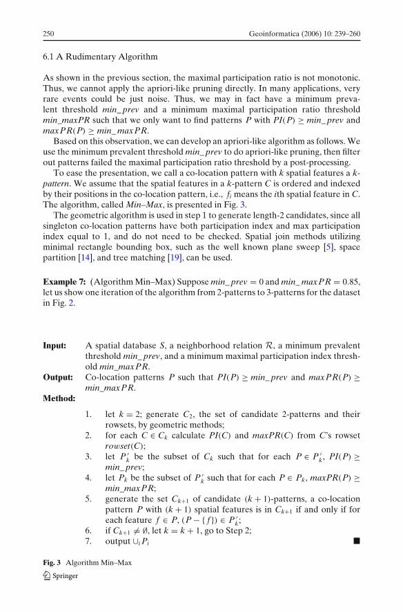
6.1 A Rudimentary Algorithm

As shown in the previous section, the maximal participation ratio is not monotonic.Thus, we cannot apply the apriori-like pruning directly. In many applications, veryrare events could be just noise. Thus, we may in fact have a minimum preva-lent threshold min_ prev and a minimum maximal participation ratio thresholdmin_maxPR such that we only want to find patterns P with PI(P) ≥ min_ prev andmaxPR(P) ≥ min_ maxPR.

Based on this observation, we can develop an apriori-like algorithm as follows. Weuse the minimum prevalent threshold min_ prev to do apriori-like pruning, then filterout patterns failed the maximal participation ratio threshold by a post-processing.

To ease the presentation, we call a co-location pattern with k spatial features a k-pattern. We assume that the spatial features in a k-pattern C is ordered and indexedby their positions in the co-location pattern, i.e., fi means the ith spatial feature in C.The algorithm, called Min–Max, is presented in Fig. 3.

The geometric algorithm is used in step 1 to generate length-2 candidates, since allsingleton co-location patterns have both participation index and max participationindex equal to 1, and do not need to be checked. Spatial join methods utilizingminimal rectangle bounding box, such as the well known plane sweep [5], spacepartition [14], and tree matching [19], can be used.

Example 7: (Algorithm Min–Max) Suppose min_ prev = 0 and min_ maxPR = 0.85,let us show one iteration of the algorithm from 2-patterns to 3-patterns for the datasetin Fig. 2.

Input: A spatial database S, a neighborhood relation R, a minimum prevalentthreshold min_ prev, and a minimum maximal participation index thresh-old min_maxPR.

Output: Co-location patterns P such that PI(P) ≥ min_ prev and maxPR(P) ≥min_maxPR.

Method:

1. let k = 2; generate C2, the set of candidate 2-patterns and theirrowsets, by geometric methods;

2. for each C ∈ Ck calculate PI(C) and maxPR(C) from C’s rowsetrowset(C);

3. let P ′k be the subset of Ck such that for each P ∈ P ′

k, PI(P) ≥min_ prev;

4. let Pk be the subset of P ′k such that for each P ∈ Pk, maxPR(P) ≥

min_maxPR;5. generate the set Ck+1 of candidate (k + 1)-patterns, a co-location

pattern P with (k + 1) spatial features is in Ck+1 if and only if foreach feature f ∈ P, (P − { f }) ∈ P ′

k;6. if Ck+1 �= ∅, let k = k + 1, go to Step 2;7. output ∪i Pi �

Fig. 3 Algorithm Min–Max

Geoinformatica (2006) 10: 239–260 251

From Table 2 , we have

P ′2 = {{A, B}, {A, C}, {A, D}, {B, C}, {B, D}, {C, D}}

and

P2 = {{A, C}, {A, D}, {B, D}, {C, D}}.From those rowsets, it is straightforward to calculate their PIs and maxPRs.The algorithm generates candidate 3-patterns C3 ={{A, B, C}, {A, B, D}, {A, C, D},{B, C, D}} from P ′

2. Then the rowsets of the candidates are generated by joining therowsets of the two 2-patterns. For example, the rowset of {A,B} joins the rowset of{A,C} to produce the rowset of {A, B, C}. At the end of this iteration, we have the setof candidate 3-patterns C3 and their rowsets. C3 is not empty. So, we start the nextround from step 2 in the algorithm. �

When the minimum prevalent threshold is set to 0, the algorithm can find thecomplete set of patterns. If min_ prev is over 0, some patterns with high maximalparticipation ratio but low prevalence may be missed. In Example 7, if min_ prev isset to 0.45, PI({A, D}) = 0.4 and {A, D} is not in P ′

2. {A, C} and {A, D} will not jointo produce candidate {A, C, D}, though max PI({A, C, D}) = 1 ≥ min_maxPR.

One advantage of the Min–Max algorithm is that the user can specify the preva-lence of patterns she wants to see by the min_ prev value. The major disadvantage ofthe algorithm is that, if a user wants to find the complete answer, the algorithm hasto generate a huge number of candidates and test them, even though the maximalparticipation ratio threshold min_maxPR is high.

6.2 Pruning by a Weak Monotonic Property

Is there any property of the maximal participation ratio we can use to get efficientalgorithms for co-location pattern mining with rare features?

Let us re-examine Example 5. Pattern P = {West Nile, poor mosquito control,domestic animal} has three proper subsets such that each subset has exactly 2features. Feature West Nile has a high participation ratio, and it participates in twoout of the three subsets. Since the participation ratio is monotonic (Lemma 1), themaximal participation ratio values of the two proper subsets containing West Nilemust be higher or equal to that of P. In other words, at most one 2-subpattern of Pcan have a lower maximal participation ratio value.

The above observation can be generalized to a pattern with l features. Thus, wehave the following weak monotonic property.

Lemma 2: (Weak monotonicity) Let P be a k-co-location pattern. Then, there existsat most one (k − 1)-subpattern P ′ such that P ′ ⊂ P and maxPR(P ′) < maxPR(P).

Proof: Let f j ∈ P be a spatial feature whose participation ratio is maximal in P. Forall (k − 1)-pattern P ′ such that (P ′ ⊂ P) ∧ (P ′ �= P/{ f j}), P ′ contains fi and fi ∈P ′ ∩ P. Based on Lemma 1, maxPR(P ′) ≥ pr(P ′, f j) ≥ pr(P, f j) = maxPR(P). Inother words, only one (k − 1)-subpattern of P, i.e., P/{ f j}, is possible to have a lowermaximal participation index value than P does. �

252 Geoinformatica (2006) 10: 239–260

Based on the above weak monotonic property, if a k-pattern is above the maximalparticipation ratio threshold, then at least (k − 1) out of its k subpatterns with (k − 1)

features are above the maximal participation ratio threshold. Therefore, we canrevise the candidate generation process, such that only a k-pattern having at mostone (k − 1)-subpattern below the minimum maximal participation ratio min_maxPRthreshold should be generated. The idea is illustrated in the following example.

Example 8: (Candidate generation using weak monotonicity) Suppose the maximalparticipation ratio values of {A, B, C}, {A, C, D} and {B, C, D} are all over thethreshold min_maxPR, but that of {A, B, D} is not. We still should generate acandidate P = {A, B, C, D}, since it is possible that maxPR(P) passes the threshold.

To achieve this, we need a systematic way to generate the candidates. Please notethat, in apriori, for the above example, {A, B, C, D} is generated only if {A, B, C}and {A, B, D} (differ only in their last spatial feature) are both frequent. However, inthe co-location pattern mining with rare spatial features using maximal participationratio measure, it is possible that {A, B, D} is below the given threshold min_maxPRwhile {A, B, C, D} is above the threshold min_maxPR.

In general, for two co-location patterns P and P ′ from the set Pk of k-patternsabove threshold min_maxPR, i.e., P ∈ Pk and P ′ ∈ Pk, P and P ′ can be joinedto generate a candidate (k + 1)-pattern in Ck+1 if and only if P and P ′ have onedifferent feature in the last two features. For example, even {A, B, D} is belowthreshold min_maxPR, candidate {A, B, C, D} can be generated by {A, B, C} and{A, C, D} since they have the common feature C in their last two features, i.e., theydiffer one spatial feature in their last two spatial features. �

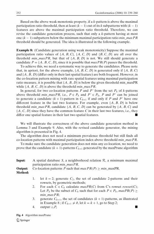
We will illustrate the correctness of the above candidate generation method inLemma 3 and Example 9. Also, with the revised candidate generator, the miningalgorithm is presented in Fig. 4.

The algorithm does not need a minimum prevalence threshold but still finds allco-location patterns with maximal participation index above threshold min_maxPR.

To make sure the candidate generation does not miss any co-location, we need toprove that the candidate (k + 1)-patterns Ck+1 generated by the maxPrune algorithm

Input: A spatial database S, a neighborhood relation R, a minimum maximalparticipation ratio min_maxPR.

Output: Co-location patterns P such that maxPR(P) ≥ min_maxPR.Method:

1. let k = 2; generate C2, the set of candidate 2-patterns and theirrowsets, by geometric methods;

2. For each C ∈ Ck calculate maxPR(C) from C’s rowset rowset(C);Let Pk be the subset of Ck such that for each P ∈ Pk, maxPR(P) ≥min_maxPR;

3. generate Ck+1, the set of candidates (k + 1)-patterns, as illustratedin Example 8 ; if Ck+1 �= ∅, let k = k + 1, go to Step 2;

4. output ∪i Pi �

Fig. 4 Algorithm maxPrune

Geoinformatica (2006) 10: 239–260 253

is a superset of the actual (k + 1)-patterns Pk+1. This is proved in the followinglemma.

Lemma 3: Let P be a k-pattern above given threshold min_maxPR (k ≥ 3). Then,there exist two (k − 1) patterns P1 and P2 such that (1) P1 ⊂ P, P2 ⊂ P, (2) P1 andP2 share their first k − 2 features, (3) P1 and P2 share either the kth or the (k − 1)thfeature or the (k − 2)th feature in P but not any two of them, and (4) both P1 and P2

are above threshold min_maxPR.

Proof: The three length-(k − 1) sub-patterns: P/{ fk−2},P/{ fk−1}, and P/{ fk} sharetheir first k − 2 features and pairwise share one feature (kth feature, (k − 1)thfeature, or (k − 2)th feature of P) in their last two features but not two of thefeatures in { fk−2, fk−1, fk}. Following Lemma 2, P has at most one length-(k − 1)

subpattern P ′ which is below threshold min_maxPR. Thus, if any one of the threebelow threshold min_maxPR, we still have the other two length-(k − 1) patterns asstated in the Lemma. �

Lemma 3 guarantees that if we generate size k candidate patterns by joining anytwo (k − 1) patterns which differ in one feature in their last two features, we will notmiss any co-location patterns above threshold min_maxI P.

Example 9: (Algorithm maxPrune) Suppose min_maxPR = 0.85. Initially, all sin-gleton co-location patterns are qualified since they have maxPR = 1. A generalgeometric method is used to generate candidate two-patterns and their rowsets. Fromtheir rowsets, we calculate their maxPR. Only the co-location patterns in

P2 = {{A, C}, {A, D}, {B, C}, {C, D}}are above min_maxPR threshold.

Then, we generate candidates 3-patterns. In detail, {A, C} joins {A, D}, {A, C}joins {B, C}, {A, C} joins {C, D}, {A, D} joins {C, D}, and {B, C} joins {C, D} togenerate candidate 3-patterns. After duplicate elimination, we have

C3 = {{A, B, C}, {A, B, D}, {A, C, D} {B, C, D}}.The rowsets of the candidates are generated by joining the rowsets of the two two-patterns leading to the candidate.

We go back to step 2. From their rowsets, we calculate the maximal participa-tion ratio values for the candidate 3-patterns. We get P3 = {{A, B, D}, {A, C, D}{B, C, D}}. The patterns in P3 are above threshold min_maxPR. Then, we generatethe candidate 4-patterns. In detail, {A, B, D} joins {A, C, D} because they differby one feature in their last two features. We thus generate candidate four-patternC4 = {A, B, C, D}, as illustrated in Example 8. Rowsets of {A, C, D} and {B, C, D}are joined to produce the rowset of {A, B, C, D}. Its maxPR is calculated and it isabove the threshold min_maxPR.

The algorithm proceeds similarly. It can be verified that C5 = ∅ and thus thealgorithm stops. �

Compared to the min–max algorithm, the maxPrune algorithm does not need anyminimum prevalence threshold and finds the complete set of co-locations above the

254 Geoinformatica (2006) 10: 239–260

minimum maximal participation index threshold min_maxPR with any prevalence.In the process of mining the complete set of these co-locations, the maxPrunealgorithm generates much less candidate co-location patterns compared to that ofmin–max with min_ prev = 0, and thus lowers down the costs of expensive rowsetgeneration and test dramatically.

7 Experimental Results

In this section, we present extensive experiments to evaluate the performance of twoalgorithms: Min–Max and maxPrune. Specifically, we test three cases: (1) data setswhich contains no co-location patterns involving rare spatial features, (2) data setscontaining patterns involving rare spatial features, and (3) large data sets.

7.1 The Experimental Setup

Our experiments were performed on synthetic data sets. We developed a datagenerator for generating synthetic data. Our data generator is similar to the oneused in [4], with some extensions to produce spatial data sets. The major parametersfor generating synthetic data sets are illustrated as follows. For a synthetic data setI100k.C10.R50, we generate 100 k instances (denoted as I100k). There are up to 50co-location patterns containing rare features with high participation ratio but verylow prevalence (denoted as R50). We achieve this by binding a spatial feature to apre-generated potential co-location pattern, and making those bound spatial featuresnot prevalent. The number of features in a co-location pattern yields to a Poissondistribution, while the mean is 10 (denoted as C10). For all generated data sets, thetotal number of features is 100 and the total number of pre-generated potential co-location patterns is 500. A summary of the parameter settings used to generate thesynthetic data sets is presented in Table 3.

We implemented algorithms min–max and maxprune using C++ and all exper-iments were performed on a Pentium III 550 MHz PC machine with 4G MB mainmemory, running Linux Redhat 6.1 operating system. Due to the space limit, we onlyreport the results on some representative data sets.

Table 3 Parameter settingsName |I| |C| |R| Size MB

I100 K.C5.R0 100K 5 0 1.86I100 K.C5.R50 5I100 K.C10.R50 100K 10 50 1.86I100 K.C15.R50 15I250 K.C5.R50 5I250 K.C10.R50 250K 10 50 4.8I250 K.C15.R50 15I750 K.C5.R50 5I750 K.C10.R50 750K 10 50 14.6I750 K.C15.R50 15I1 M.C5.R50 5I1 M.C10.R500 1M 10 50 19.6I1 M.C15.R50 15

Geoinformatica (2006) 10: 239–260 255

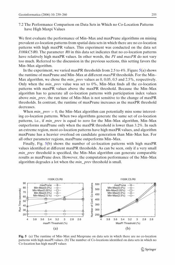
7.2 The Performance Comparison on Data Sets in Which no Co-Location Patternshave High Maxpi Values

We first evaluate the performance of Min–Max and maxPrune algorithms on miningprevalent co-location patterns from spatial data sets in which there are no co-locationpatterns with high maxPR values. This experiment was conducted on the data setI100kC5R0. The parameter R0 in this data set indicates that no co-location patternshave relatively high maxPR values. In other words, the PI and maxPR do not varytoo much. Referred to the discussion in the previous sections, this setting favors theMin–Max algorithm.

In the experiment, we varied maxPR thresholds from 2.5 to 4%. Figure 5(a) showsthe runtime of maxPrune and Min–Max at different maxPR thresholds. For the Min–Max algorithm, we chose the min_ prev values as 0, 0.05, 0.5 and 2.5%, respectively.Only when the min_ prev value was set to 0%, Min–Max finds all the co-locationpatterns with maxPR values above the maxPR threshold. Because the Min–Maxalgorithm has to generate all co-location patterns with participation index valuesabove min_ prev, the run time of Min–Max is not sensitive to the change of maxPRthresholds. In contrast, the runtime of maxPrune increases as the maxPR thresholddecreases.

When min_ prev > 0, the Min–Max algorithm can potentially miss some interest-ing co-location patterns. When two algorithms generate the same set of co-locationpatterns, i.e., if min_ prev is equal to zero for the Min–Max algorithm, Min–Maxoutperforms maxPrune only when the maxPR threshold is lower than 3.2%. In suchan extreme region, most co-location patterns have high maxPR values, and algorithmmaxPrune has a heavier overload on candidate generation than Min–Max has. Forall other parameter regions, maxPrune outperforms Min–Max.

Finally, Fig. 5(b) shows the number of co-location patterns with high maxPRvalues identified at different maxPR thresholds. As can be seen, only if a very smallmin_ prev threshold is specified, the Min–Max algorithm can generate comparableresults as maxPrune does. However, the computation performance of the Min–Maxalgorithm degrades a lot when the min_ prev threshold is small.

Fig. 5 (a) The runtime of Min–Max and Maxprune on data sets in which there are no co-locationpatterns with high maxPI values. (b) The number of Co-locations identified on data sets in which noCo-location has high maxPI values

256 Geoinformatica (2006) 10: 239–260

Fig. 6 (a) The runtime of Min–Max and maxPrune on data sets containing co-locations with highmaxPR values. (b) The number of co-location patterns identified on data sets containing co-locationswith high maxPI values

7.3 Performance Comparison on Data Sets Containing Co-Location Patterns withHigh Maxpi Values

Here, we compare the performance of maxPrune and Min–Max on a data set(I100K.C5.R50) in which there are many co-location patterns with high maxPR val-ues but low prevalence. In this experiment, we identified many co-location patternswith relatively high maxPR values, say above 50%.

Figure 6(a) shows the runtime of Min–Max and maxPrune on data setI100K.C5.R50. As can be seen, the runtime of Min–Max dramatically increases withthe decrease of participation index thresholds. In contrast, the runtime of maxPruneis not affected by the change of participation index thresholds and is much smallerthan that of Min–Max with respect to different MaxPI thresholds. In addition,Fig. 6(b) shows that the number of co-location patterns identified by Min–Maxdecreases with the increase of participation index thresholds. In other words, for themin–max algorithm, there is a trade-off between the efficiency and the completenessof results. However, the maxPrune algorithm does not have such a dilemma situation.

Fig. 7 (a) Scalability of the maxPrune algorithm w.r.t. maxPR. threshold (b) Scalability of themaxPrune algorithm w.r.t. number of instances

Geoinformatica (2006) 10: 239–260 257

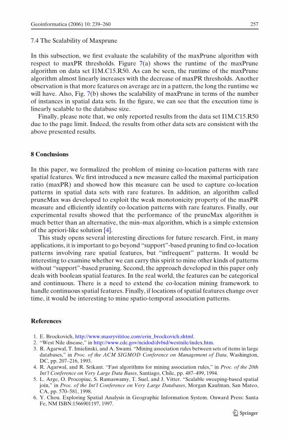
7.4 The Scalability of Maxprune

In this subsection, we first evaluate the scalability of the maxPrune algorithm withrespect to maxPR thresholds. Figure 7(a) shows the runtime of the maxPrunealgorithm on data set I1M.C15.R50. As can be seen, the runtime of the maxPrunealgorithm almost linearly increases with the decrease of maxPR thresholds. Anotherobservation is that more features on average are in a pattern, the long the runtime wewill have. Also, Fig. 7(b) shows the scalability of maxPrune in terms of the numberof instances in spatial data sets. In the figure, we can see that the execution time islinearly scalable to the database size.

Finally, please note that, we only reported results from the data set I1M.C15.R50due to the page limit. Indeed, the results from other data sets are consistent with theabove presented results.

8 Conclusions

In this paper, we formalized the problem of mining co-location patterns with rarespatial features. We first introduced a new measure called the maximal participationratio (maxPR) and showed how this measure can be used to capture co-locationpatterns in spatial data sets with rare features. In addition, an algorithm calledpruneMax was developed to exploit the weak monotonicity property of the maxPRmeasure and efficiently identify co-location patterns with rare features. Finally, ourexperimental results showed that the performance of the pruneMax algorithm ismuch better than an alternative, the min–max algorithm, which is a simple extensionof the apriori-like solution [4].

This study opens several interesting directions for future research. First, in manyapplications, it is important to go beyond “support”-based pruning to find co-locationpatterns involving rare spatial features, but “infrequent” patterns. It would beinteresting to examine whether we can carry this spirit to mine other kinds of patternswithout “support”-based pruning. Second, the approach developed in this paper onlydeals with boolean spatial features. In the real world, the features can be categoricaland continuous. There is a need to extend the co-location mining framework tohandle continuous spatial features. Finally, if locations of spatial features change overtime, it would be interesting to mine spatio-temporal association patterns.

References

1. E. Brockovich, http://www.masryvititoe.com/erin_brockovich.shtml.2. “West Nile disease,” in http://www.cdc.gov/ncidod/dvbid/westnile/index.htm.3. R. Agarwal, T. Imielinski, and A. Swami. “Mining association rules between sets of items in large

databases,” in Proc. of the ACM SIGMOD Conference on Management of Data, Washington,DC, pp. 207–216, 1993.

4. R. Agarwal, and R. Srikant. “Fast algorithms for mining association rules,” in Proc. of the 20thInt’l Conference on Very Large Data Bases, Santiago, Chile, pp. 487–499, 1994.

5. L. Arge, O. Procopiuc, S. Ramaswamy, T. Suel, and J. Vitter. “Scalable sweeping-based spatialjoin,” in Proc. of the Int’l Conference on Very Large Databases, Morgan Kaufman, San Mateo,CA, pp. 570–581, 1998.

6. Y. Chou. Exploring Spatial Analysis in Geographic Information System. Onward Press: SantaFe, NM ISBN:1566901197, 1997.

258 Geoinformatica (2006) 10: 239–260

7. N.A.C. Cressie. Statistics for Spatial Data. Wiley: New York ISBN:0471843369, 1991.8. Environmental Systems Research Institute, Inc. “ArcGIS Family,” in http://www.esri.com.9. M. Ester, A. Frommelt, H.-P. Kriegel, and J. Sander. “Algorithms for characterization and trend

detection in spatial databases,” in Proc. of the ACM SIGKDD International Conference onKnowledge Discovery and Data Mining, New York, pp. 44–50, 1998.

10. V. Estivill-Castro, and I. Lee. “Data mining techniques for autonomous exploration of largevolumes of geo-referenced crime data,” in Proc. of the 6th International Conference onGeocomputation, pp. 24–26, 2001.

11. V. Estivill-Castro, and A. Murray. “Discovering associations in spatial Data—an efficient medoidbased approach,” in Proc. of the Second Pacific-Asia Conference on Knowledge Discovery andData Mining, Springer, Berlin Heidelberg New York, pp. 110–121, 1998.

12. R.H. Guting. “An introduction to spatial database systems,” Very Large Data Bases Journal, Vol.3: 357–399, 1994.

13. Y. Huang, H. Xiong, S. Shekhar, and J. Pei. “Mining confident co-location rules without asupport threshold,” in Proceedings of the 18th Annual ACM Symposium on Applied Computing(SAC’03), Melbourne, Florida, pp. 497–418, 2003.

14. J. M. Patel, and D. J. DeWitt. “Partition based spatial-merge join,” in Proc. of the ACMSIGMOD Conference on Management of Data, pp. 259–270, 1996.

15. E. M. Knorr, R. T. Ng, and D. L. Shilvock. “Finding boundary shape matching relationshipsin spatial data,” in Proc. 5th International Symposium on Spatial Databases, Springer, BerlinHeidelberg New York, pp. 29–46, 1997.

16. K. Koperski, J. Adhikary, and J. Han. “Spatial data mining: Progress and challenges,” inWorkshop on Research Issues on Data Mining and Knowledge Discovery, pp. 409–418, OxfordUniversity Press, UK, 1996.

17. K. Koperski, and J. Han. “Discovery of spatial association rules in geographic informationdatabases,” in Proc. of the 4th International Symposium on Spatial Databases, Springer, BerlinHeidelberg New York, pp. 47–66, 1995.

18. M. Koubarakis, T.K. Sellis, A.U. Frank, S.Grumbach, R.H. Güting, C.S. Jensen, N.A. Lorentzos,Y. Manolopoulos, E. Nardelli, B. Pernici, H.-J. Schek, M.Scholl, B. Theodoulidis, and N. Tryfona.Spatio-Temporal Databases: The CHOROCHRONOS Approach. Springer: Berlin HeidelbergNew York, 2003.

19. S.T. Leutenegger, and M.A. Lopez. “The Effect of buffering on the performance of R-trees,”in Proc. of the Int’l Conference on Data Engineering, IEEE Educational Activities Department,pp. 164–171, 1998.

20. Y. Morimoto. “Mining frequent neighboring class sets in spatial databases,” in Proc. ACMSIGKDD International Conference on Knowledge Discovery and Data Mining, ACM, pp. 353–358, 2001.

21. R. Munro, S.Chawla, P. Sun. “Complex spatial relationships,” The Third IEEE InternationalConference on Data Mining (ICDM2003), IEEE Computer Society, p. 227, 2003.

22. R. T. Ng, and J. Han. “Efficient and effective clustering methods for spatial data mining,” in20th International Conference on Very Large Data Bases, Morgan Kaufman, San Mateo, CA,pp. 144–155, 1994.

23. J.F. Roddick, and M. Spiliopoulou. “A bibliography of temporal, spatial and spatio-temporaldata mining research,” in ACM Special Interest Group on Knowledge Discovery in Data MiningExplorations, New York, pp. 34–38, 1999.

24. S. Shekhar, and S. Chawla. Spatial Databases: A Tour. Prentice Hall: New Jersey ISBN:0130174807, 2003.

25. S. Shekhar, S. Chawla, S. Ravada, A. Fetterer, X. Liu, and C.T. Lu. “Spatial databases: Accom-plishments and research needs,” IEEE Trans. Knowl.Data Eng., Vol. 11(1):45–55, 1999.

26. S. Shekhar, and Y. Huang. “Co-location rules mining: A summary of results,” in Proc. 7th Intl.Symposium on Spatio-temporal Databases, Springer, Berlin Heidelberg New York, p.236, 2001.

27. S. Shekhar, C.T. Lu, and P. Zhang. “Detecting graph-based spatial outliers: Algorithms andapplications,” in The Seventh ACM SIGKDD Intl. Conf. on Knowledge Discovery and DataMining, San Francisco,California, pp. 371–376, 2001.

28. S. Shekhar, P. Schrater, W.R. Raju, W. Wu, and S. Chawla. “Spatial contextual classificationand prediction models for mining geospatial data,” in IEEE Transactions on Multimedia: SpecialIssue on Multimedia Databases, IEEE Trans. Multimedia, pp. 174–188, 2002.

29. W. Wang, J. Yang, and R. Muntz. “STING: A statistical information grid approach to spatialdata mining” in International Conference on Very Large Data Bases, Athens, Greece, MorganKaufman, San Mateo, CA, pp. 186–195, 1997.

Geoinformatica (2006) 10: 239–260 259

30. M.F. Worboys. GS: A Computing Perspective. Taylor and Francis: New York 1995.31. X. Zhang, N. Mamoulis, D.W.L Cheung, and Y. Shou. “Fast mining of spatial collocations,” in

Proc. of the ACM SIGKDD International Conference on Knowledge Discovery and Data Mining,Seattle, pp. 384–393, 2004.

Yan Huang received her B.S. degree in Computer Science from Beijing University, Beijing, China,in July 1997 and Ph.D. degree in Computer Science from University of Minnesota, Twin-cities, MN,USA, in July 2003. She is currently an assistant professor at the Computer Science and EngineeringDepartment of University of North Texas, Denton, TX, USA. Her research interests include sensornetworked databases, scientific databases, data mining, and geographic information systems (GIS).She has published over 20 technical papers in peer-reviewed journals and conference proceedings.She has served on the program committees for a number of conferences and workshops, and has beena reviwer for several journals. She is a recipient of a Ralph E. Powe Junior Faculty EnhancementAwards from ORNL Oak Ridge Associated Universities and is a member of the IEEE ComputerSociety, the ACM, and the ACM SIGMOD.

Jian Pei received the Ph.D. degree in Computing Science from Simon Fraser University, Canada,in 2002. He is currently an Assistant Professor of Computing Science at Simon Fraser University,Canada. His research interests can be summarized as developing effective and efficient data analysistechniques for novel data intensive applications. Particularly, he is currently interested in varioustechniques of data mining, data warehousing, online analytical processing, and database systems,as well as their applications in bioinformatics. His current research is supported in part by theNatural Sciences and Engineering Research Council of Canada (NSERC) and the National ScienceFoundation (NSF) of the United States. Since 2000, he has published over 70 research papers inrefereed journals, conferences, and workshops, has served in the organization committees and theprogram committees of over 60 international conferences and workshops, and has been a reviewerfor some leading academic journals. He is a member of the ACM, the ACM SIGMOD, the ACMSIGKDD, the IEEE Computer Society.

260 Geoinformatica (2006) 10: 239–260

Hui Xiong is an assistant professor in the Management Science and Information Systems depart-ment at Rutgers, the State University of New Jersey. He received the B.E. degree in Automationfrom the University of Science and Technology of China, China, the M.S. degree in ComputerScience from the National University of Singapore, Singapore, and the Ph.D. degree in ComputerScience from the University of Minnesota, MN, USA. His research interests include data mining,statistical computing, Geographic Information Systems (GIS), Biomedical informatics, and informa-tion security. He has published over 20 technical papers in peer-reviewed journals and conferenceproceedings and is the co-editor of the book entitled “Clustering and Information Retrieval”. He hasalso served on the program committees for a number of conferences and workshops. Dr. Xiong is amember of the IEEE Computer Society, the ACM, the ACM SIGKDD, and Sigma Xi.