Embed Size (px)
Citation preview
MINING AND VISUALIZATION OF ASSOCIATION RULESOVER RELATIONAL DBMSs
By
HONGEN ZHANG
A THESIS PRESENTED TO THE GRADUATE SCHOOLOF THE UNIVERSITY OF FLORIDA IN PARTIAL FULFILLMENT
OF THE REQUIREMENTS FOR THE DEGREE OFMASTER OF SCIENCE
UNIVERSITY OF FLORIDA
2000

To my family

iii
ACKNOWLEDGMENTS
I thank all the people who may be related to this research directly and indirectly.
Special gratitude should be given to my advisor, Dr. Sharma Chakravarthy, for his
excellent advice and support in this research. His tireless patience and great
understanding of data mining are the keys for the success of this thesis. I am grateful to
Dr. Stanley Su and Dr. Joachim Hammer for agreeing to serve on my supervisory
committee, for teaching great classes that have helped me in the understanding of
database, and for reading and commenting on my thesis.
I would also like to thank Sharon Grant for maintaining a very nice research
environment. She takes care of everything and she is always available in times of need.
Special thanks go to Mahesh Dudgikar for discussions related to this research project.
The most appreciation from me should be given to my family for their endless
love. They always encouraged me during times of difficulty. Without their support, this
work would not have been possible.

iv
TABLE OF CONTENTS
page
ACKNOWLEDGMENTS..................................................................................................iii
LIST OF TABLES ............................................................................................................vii
LIST OF FIGURES............................................................................................................ ix
ABSTRACT ......................................................................................................................xii
CHAPTERS
1 INTRODUCTION........................................................................................................... 1
1.1 Categories of Data Mining ........................................................................................11.1.1 Association Rule ................................................................................................11.1.2 Clustering ...........................................................................................................31.1.3 Classification......................................................................................................31.1.4 Sequential Patterns .............................................................................................51.1.5 Text Mining........................................................................................................61.1.6 Active Data Mining ............................................................................................7
1.2 Problem Statement ....................................................................................................71.3 Thesis Organization.................................................................................................10
2 ARCHITECTURE AND FEATURES OF JDBC AND ORACLE .............................. 12
2.1 JDBC .......................................................................................................................122.2 Features of Oracle ...................................................................................................14
3 ALTERNATIVE APPROACHES TO ASSOCIATION RULE MINING................... 18
3.1 Related Work...........................................................................................................183.1.1 Apriori Algorithm ............................................................................................183.1.2 Architectural Alternatives ................................................................................19
3.1.2.1 Cache-Mine ...............................................................................................193.1.2.2 SQL-based Approach ................................................................................203.1.2.3 Integrated Approach ..................................................................................21
3.2 Support Counting ....................................................................................................223.2.1 Candidate Set Generation.................................................................................223.2.2 SQL 92 .............................................................................................................24
v
3.2.2.1 K-Way Join ...............................................................................................243.1.2.2 2-GroupBy.................................................................................................253.1.2.3 Sub-Query .................................................................................................26
3.2.3 SQL-OR............................................................................................................283.2.3.1 Vertical ......................................................................................................283.2.3.2 GatherJoin .................................................................................................333.2.3.3 GatherJoin Variant ....................................................................................37
3.3 Rule Generation.......................................................................................................393.3.1 Intermediate Rule Generation ..........................................................................393.3.2 Mapping Back Process .....................................................................................42
3.4 Performance Testing................................................................................................433.4.1 Synthetic Data Generation................................................................................433.4.2 Performance of SQL-92 and SQL-OR Approaches and Intelligent Miner ......443.4.3 Scale-Up Experiments......................................................................................47
4 VISUALIZATION OF ASSOCIATION RULES......................................................... 48
4.1 Related Work...........................................................................................................484.1.1 Classification of Data Visualization Techniques .............................................494.1.2 Rule Table ........................................................................................................504.1.3 2-D and 3-D Rule Visualization.......................................................................50
4.1.3.1 Directed Graph ..........................................................................................514.1.3.2 2-D Matrix.................................................................................................524.1.3.3 3-D Visualization ......................................................................................54
4.2 Rule Table ...............................................................................................................554.3 3-D Visualization ....................................................................................................57
5 SYSTEM IMPLEMENTATION .................................................................................. 62
5.1 System Architecture ................................................................................................645.2 Main Window..........................................................................................................655.3 LogIn Module..........................................................................................................665.4 Rule Generator ........................................................................................................705.5 Visualization Module ..............................................................................................72
5.5.1 Rule Table ........................................................................................................725.5.2 3-D Visualization .............................................................................................76
6 CONCLUSION AND FUTURE WORK...................................................................... 86
6.1 Conclusion...............................................................................................................866.2 Contributions...........................................................................................................886.3 Future Work ............................................................................................................88
APPENDIX ASSOCIATION RULE MINING EXAMPLE USING KWAY JOIN........ 90
LIST OF REFERENCES .................................................................................................. 97
vi
BIOGRAPHICAL SKETCH........................................................................................... 100

vii
LIST OF TABLES
Table Page
1.1 Example Basket Data Set ............................................................................................... 2
1.2 Example Training Set..................................................................................................... 4
1.3 Sequences of an Example Database ............................................................................... 5
2.1 TIDITEM Table ............................................................................................................. 16
2.2 tidT Table ....................................................................................................................... 17
3.1 Table TIDT Contains All Tids and Count for Each Item............................................... 29
3.2 Table TITEM Contains All Items and Count for each Tid ............................................ 33
3.3 Frequent Item Sets Table ‘FISETS’ ............................................................................... 39
3.4 Table ‘Primary-Rules’.................................................................................................... 40
3.5 Table ‘Rules’ .................................................................................................................. 41
3.6 Example of “Description” Table .................................................................................... 42
3.7 Synthetic Data Sets......................................................................................................... 44
4.1 Example of Association Rules in Rule Table Format .................................................... 50
4.2 Example of Association Rules in Rule Table Format .................................................... 55
A-1 Example of Input Data Set ............................................................................................ 90
A-2 Example of Description Table ...................................................................................... 91
A-3 TIDITEM Table ............................................................................................................ 91
A-4 Table “C1” ..................................................................................................................... 92
A-5 Table “F1”...................................................................................................................... 92

viii
A-6 Table “C2” ..................................................................................................................... 93
A-7 Table “F2”...................................................................................................................... 93
A-8 Table “C3” ..................................................................................................................... 93
A-9 Table “F3”...................................................................................................................... 94
A-10 Frequent Item Sets “FISETS” ..................................................................................... 94
A-11 Table “Primary-Rules”................................................................................................ 95
A-12 Table “Rules” .............................................................................................................. 95
A-13 Final “Association Rules” ........................................................................................... 96
ix
LIST OF FIGURES
Figure Page
1.1 Decision Tree ................................................................................................................. 4
1.2 Active Data Mining........................................................................................................ 8
2.1 Architecture of Two-tier Model ..................................................................................... 13
2.2 Architecture of Three-tier Model ................................................................................... 13
2.3 Architecture of JDBC..................................................................................................... 14
2.4 PL/SQL Stored procedure “SaveTid” ............................................................................ 16
3.1 Apriori Algorithm .......................................................................................................... 19
3.2 Cache-Mine Architecture ............................................................................................... 20
3.3 SQL-based Architecture ................................................................................................. 21
3.4 Architecture for the Integrated Approach ...................................................................... 22
3.5 SQL Query for Candidate Sets Ck.................................................................................. 22
3.6 Prune step for Candidate Sets Ck.................................................................................... 23
3.7 The Query of Candidate Set Generation and Pruning.................................................... 24
3.8 Query Diagram and SQL Query of K-Way Join............................................................ 25
3.9 Query of 2-GroupBy ...................................................................................................... 26
3.10 Query Diagram and SQL Query of Sub-Query............................................................ 27
3.11 PL/SQL Stored Procedure SaveTid() ........................................................................... 30
3.12 Stored Procedure CountAnd2()..................................................................................... 32
3.13 Oracle Stored Procedure SaveItem()............................................................................ 34
x
3.14 Oracle Stored Procedure Comb2()................................................................................ 36
3.15 Support Counting of GathorJoin .................................................................................. 37
3.16 Support Counting of GathorJoin Variant ..................................................................... 38
3.17 Association Rules Generation Query ........................................................................... 41
3.18 Performance Comparison of SQL-92 Approaches and Intelligent Miner for Data SetT5D10K............................................................................................................... 45
3.19 Performance Comparison of SQL-92 Approaches and Intelligent Miner for Data SetT5D100K............................................................................................................. 46
3.20 Performance Comparison of SQL-92 Approaches and Intelligent Miner for Data SetT10D10K............................................................................................................. 46
3.21 Scale-Up Experiments for SQL-92 Approaches .......................................................... 47
4.1 Association Rules Represented by Directed Graph ....................................................... 51
4.2 Association Rules Represented by 2-D matrix .............................................................. 52
4.3 Association Rules Represented by 2-D Matrix .............................................................. 53
4.4 Multiple Items in Rule Head .......................................................................................... 54
4.5 3-D Visualization of Association Rules ......................................................................... 56
4.7 Association Rules that have more than 1 Item in Rule Body......................................... 59
4.8 Association Rule Visualization ...................................................................................... 61
5.1 System Architecture ....................................................................................................... 65
5.2 Main Window of Association Rule Software................................................................. 66
5.3 Login Window of Association Rule Software ............................................................... 68
5.4 btnConnect_actionPerformed Method ........................................................................... 69
5.5 Parameter Input Window of Association Rule Software ............................................... 71
5.6 Retrieve All the Table Names Available in the Database .............................................. 72
5.7 Rule Table Visualization Window with Filter Function ................................................ 74
5.8 Show_Rule Method........................................................................................................ 74
xi
5.9 Rule Table Visualization Window with Sort Function .................................................. 75
5.10 Different Categories of Rules Based on # of Items in the Rule Head.......................... 77
5.11 Options Window in Association Rule Software .......................................................... 78
5.12 Constraints Window in Association Rule Software..................................................... 79
5.13 3-D Visualization Window in Association Rule Software........................................... 80
5.14 Simple Recipe for Writing Java 3D Programs using SimpleUniverse......................... 81
5.15 Paint Method in ThreeD_General Class....................................................................... 82
5.16 Content Branch for Items in the Rule Head of All Rules............................................. 84
xii
Abstract of Thesis Presented to the Graduate Schoolof the University of Florida in Partial Fulfillment of the
Requirements for the Degree of Master of Science
MINING AND VISUALIZATION OF ASSOCIATION RULESOVER RELATIONAL DBMSs
By
Hongen Zhang
August 2000
Chairman: Sharma ChakravarthyMajor Department: Computer and Information Science and Engineering
As more and more data are collected and stored in multiple databases, data mining
over different relational DBMSs is becoming increasingly important. Usually the data
sets are stored in some different DBMSs, such as DB2, Oracle, Sybase, etc. Data mining
software should be able to use the data from all of these DBMSs. In this thesis we use
JDBC (Java Database Connectivity) to achieve this goal. The test DBMSs we used are
Oracle and DB2.
We implement the association rule algorithm in the form of SQL queries. Three
algorithms in SQL-92 (K-Way Join, 2-Groupby, and Subquery) and three algorithms in
SQL-OR (Vertical, GatherJoin and GatherJoin Variant) are implemented and compared
to each other based on their performance on different kinds of synthetic generated data
sets. Scale-Up experiments have also been conducted for these six approaches.
xiii
We develop an association rule visualization system, which includes tabular form
and three-dimensional graphics. By providing the user sorting and filtering abilities, this
rule visualization system makes it flexible and efficient for the user to manage and
understand the association rules. As a result, this visualization system becomes an
essential part of our association rule software.
Finally, we compare our association rule software with one of the commercial
data mining tools (Intelligent Miner from IBM) in various aspects, such as data
accessibility, user interface, input/output, and rule visualization.

1
CHAPTER 1INTRODUCTION
As computers are used in more and more areas, large volumes of data have been
collected and stored in the database continuously. This kind of data includes the
transaction records in supermarkets, banks, stock markets, and telephone companies.
With the increasing volume of the stored data, an important issue is to figure out how to
find the useful information from these massive history data. Data mining, also known as
knowledge discovery in databases, is such a research area to extract implicit,
understandable, previously unknown and potentially useful information from data. In
Section 1.1 we briefly describe different categories of data mining, such as association
rule, clustering, classification, sequential pattern, text mining and active data mining. The
limitations of currently available commercial data mining software (especially for
association rule) are discussed in Section 1.2 and in Section 1.3, we outline the thesis
organization.
1.1 Categories of Data Mining
1.1.1 Association Rule
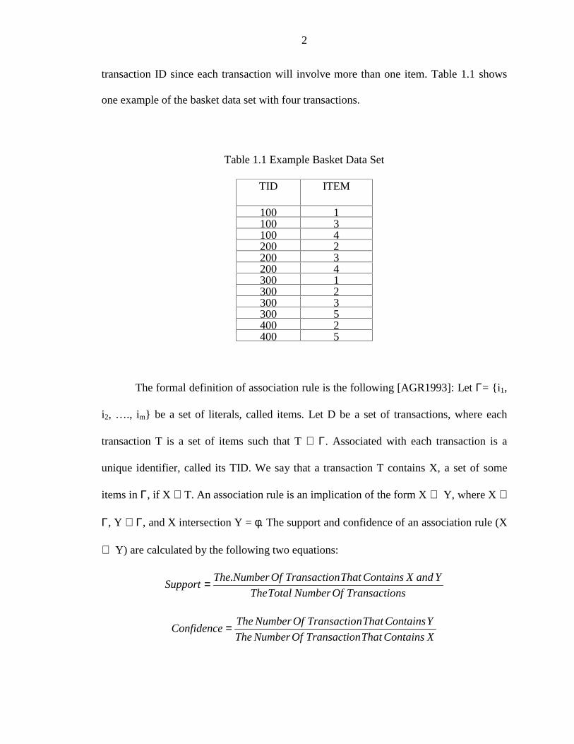
The typical example of association rule is the Basket data analysis [AGR1994]. In
a given database D, all the records consist of two attributes: transaction ID (TID), and the
item the customer bought in the transaction. Usually the item attribute in each record
contains only one item, so in the database, there will be more than one row for a
2
transaction ID since each transaction will involve more than one item. Table 1.1 shows
one example of the basket data set with four transactions.
Table 1.1 Example Basket Data Set
TID ITEM
100 1100 3100 4200 2200 3200 4300 1300 2300 3300 5400 2400 5
The formal definition of association rule is the following [AGR1993]: Let Γ= {i1,
i2, …., im} be a set of literals, called items. Let D be a set of transactions, where each
transaction T is a set of items such that T ⊆ Γ. Associated with each transaction is a
unique identifier, called its TID. We say that a transaction T contains X, a set of some
items in Γ, if X ⊆ T. An association rule is an implication of the form X ⇒ Y, where X ⊂
Γ, Y ⊂ Γ, and X intersection Y = φ. The support and confidence of an association rule (X
⇒ Y) are calculated by the following two equations:
nsTransactioOfNumberTotalThe
YandXContainsThatnTransactioOfNumberTheSupport
.=
XContainsThatnTransactioOfNumberThe
YContainsThatnTransactioOfNumberTheConfidence =
3
The rule X ⇒ Y holds in the transaction set D if its support and confidence are
equal to or greater than the user specified values. The goal of association rules is to find
the relationship between any combination of items.
1.1.2 Clustering
The goal of clustering is to identify homogeneous groups of objects based on the
values of their attributes [AGR1998]. For a given set of objects (each object has several
attributes), the task of clustering is to group some objects together (we call these objects
are in one cluster) so that the objects in the same cluster are more similar to each other
than to objects in a different cluster. The technique of solving clustering problems falls
into two categories: partitional and hierarchical [AGR1998]. For the partitional
clustering, the K-means method is widely used. This method first determines K cluster
representatives, then assign each object to the cluster with its representative closest to the
object such that the sum of the distances squared between the objects and their
representatives is minimized. For the hierarchical clustering, it usually starts by placing
each object in its own cluster and then merges these atomic clusters into larger and larger
clusters until all objects are in a single cluster.
1.1.3 Classification
The classification problem can be described as the following [MEH1996]: For a
given database D, each record consists of several attributes. Among all the attributes, one
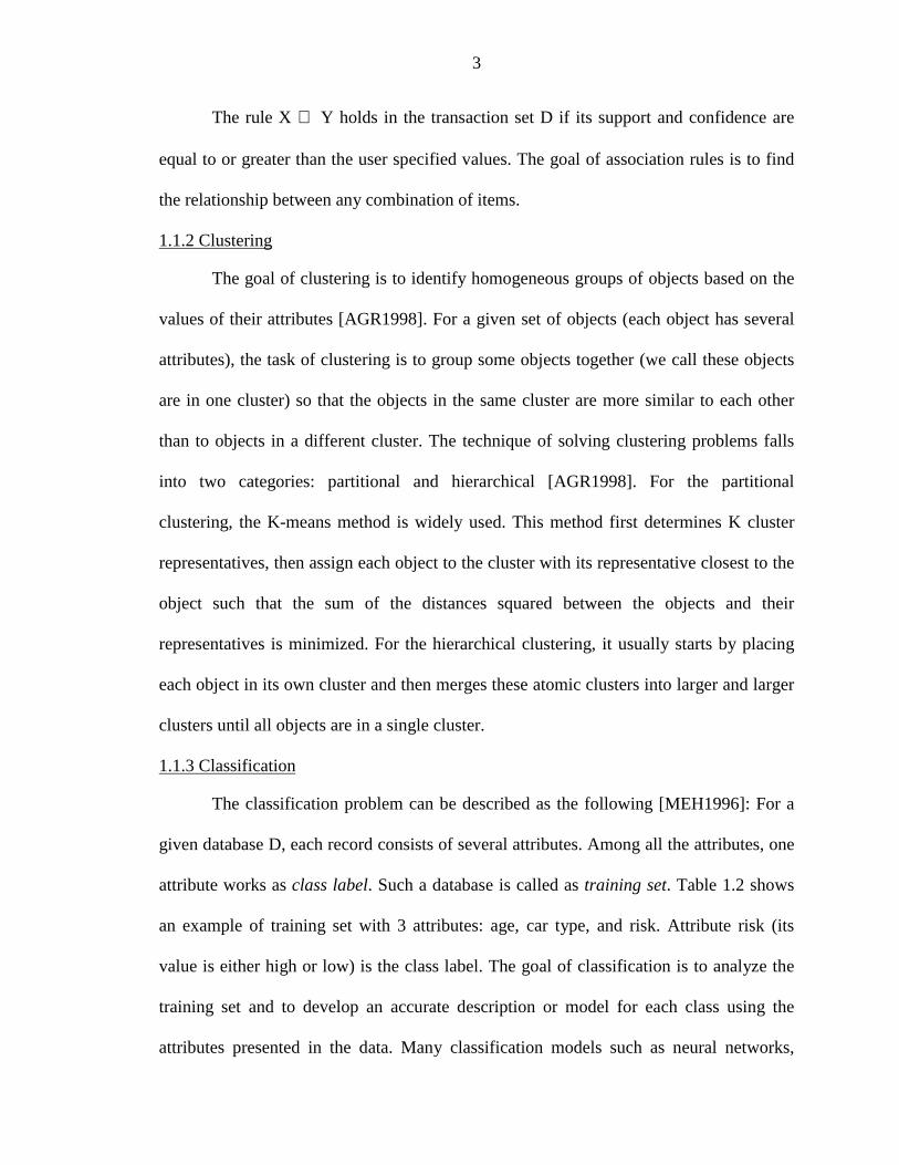
attribute works as class label. Such a database is called as training set. Table 1.2 shows
an example of training set with 3 attributes: age, car type, and risk. Attribute risk (its
value is either high or low) is the class label. The goal of classification is to analyze the
training set and to develop an accurate description or model for each class using the
attributes presented in the data. Many classification models such as neural networks,
4
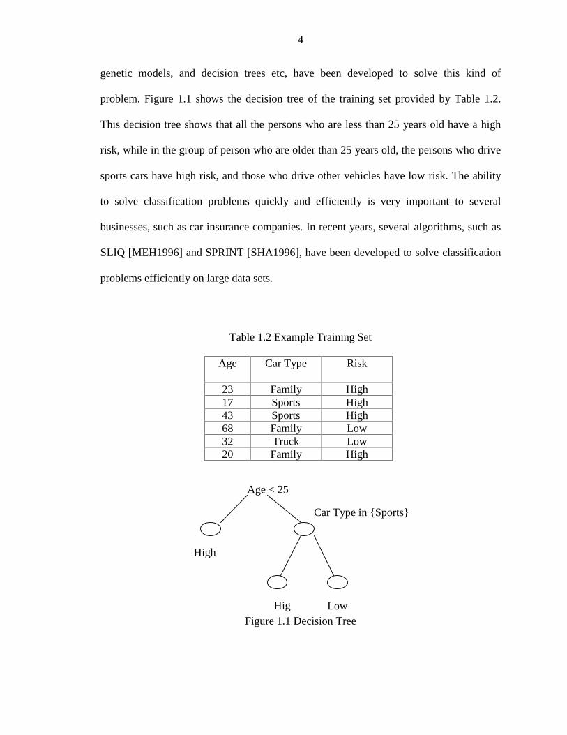
genetic models, and decision trees etc, have been developed to solve this kind of
problem. Figure 1.1 shows the decision tree of the training set provided by Table 1.2.
This decision tree shows that all the persons who are less than 25 years old have a high
risk, while in the group of person who are older than 25 years old, the persons who drive
sports cars have high risk, and those who drive other vehicles have low risk. The ability
to solve classification problems quickly and efficiently is very important to several
businesses, such as car insurance companies. In recent years, several algorithms, such as
SLIQ [MEH1996] and SPRINT [SHA1996], have been developed to solve classification
problems efficiently on large data sets.
Table 1.2 Example Training Set
Age Car Type Risk
23 Family High17 Sports High43 Sports High68 Family Low32 Truck Low20 Family High
Figure 1.1 Decision Tree
Age < 25
High
Car Type in {Sports}
Hig Low

5
1.1.4 Sequential Patterns
The formal definition of sequential patterns is given in Agrawal and Srikant
[AGR1995c]. For a given database D, which consists of customer transactions. Each
transaction consists of the following fields: customer-ID, transaction-time, and the items
purchased in the transaction. An item-set is a non-empty set of items, and a sequence is
an order list of item-sets. We say a sequence A <a1, a2, a3, …, an> is contained in another
sequence B <b1, b2, b3, …, bn> if there exist integers i1<i2<i3<…<in, such that a1⊆ bi1,
a2⊆ bi2, …, an⊆ bin. For example, the sequence < (3) (4,5) (8)> is contained in <(7) (3,8)
(9) (4,5,6) (8)>, because (3) ⊆ (3,8), (4,5) ⊆ (4,5,6), and (8) ⊆ (8). A customer sequence is
a sequence of item-sets for each customer-ID. The support of a sequence s is defined by
the following equation:
SequencesofNumberTotal
SequenceThisContainsThatSequenceofNumberTheSupport =
For the example data set in Table 1.3, We can find all the sequences that have
support > 25%, which are < (30) (90) >, and < (30) (40,70) >.
Table 1.3 Sequences of an Example Database
Customer Customer Sequence1 < (30) (90) >2 < (10, 20) (30) (40, 60, 70) >3 < (30,50,70) >4 < (30) (40,70) (90) >5 < (90) >
The goal of sequential patterns is to find the sequences that have greater than or
equal to a certain user pre-specified support. Usually the process of finding sequential

6
patterns consists of the following phases: sorting phase, finding the large item-set phase,
transformation phase, sequence phase, and maximal phase.
1.1.5 Text Mining
In the real world, it is very common to find the hidden relationship in the larger
text database. For example, it is very useful to find whether the company is shifting its
interest from one domain to another. Text mining is very good at handling this situation
since the database in full of text, instead of the numeric data. The goal of text mining is to
discover the trends in the text database. Lent et al. [LEN1997] developed a system to
discover the trends in text database. Their basic idea is to use the existing data mining
algorithms and shape query language (SDL) [AGR1995b]. For a given database D of
documents (each document consists of text fields and a timestamp, the unit of text is a
word and a phrase is a list of words), they begin with cleansing and parsing the data, and
then separating the documents based on their timestamp. Each word will be assigned a
transaction ID based on its document timestamp. Then the sequential pattern algorithm
will be applied for the transformed data to produce the results. The results will be queried
using shape query to find the increasing or decreasing trend of the occurrence frequency.
The purpose of using shape query language is that a “blurry” match (cares about the
overall shape, but not the specific details) is possible. The following is an example of
shape query language:
(in 5 (and (no less 2 (any up Up)) (no more 1 (any down Down))))
This statement shows that we are interested in the subsequences five intervals
long that have at least two ups (either up or Up) and at most one down (either down or
Down).
7
1.1.6 Active Data Mining
Active data mining combines the technology of data mining and active database.
The basic idea [AGR1995a] is to divide the whole data into several sub-data sets. The
data mining algorithms will be applied to each sub-data set and the results for each sub-
data set will be produced. Because usually the data sets come from data warehousing and
thus the volume of data is very huge, dividing the data set to several sub-data sets will not
lose the significance of the results. All the rules generated in each sub-data set will be
stored in the rule database with some parameters, such as the support and confidence for
association rule problems. When the new data comes in, and the volume of new data
reached a certain level, the data mining algorithm will be applied to the new data set
again and then check the rule database. If one certain rule does not exist, it just stores the
rule into the rule database. If this rule exists in the rule database, it will update the
parameters of the existing rules in the rule database. The database uses trigger to monitor
the parameters in the rule database. Once the condition is met, the specific trigger will be
fired. ECA (Event Condition Action) model [CHA1995] can be used for more complex
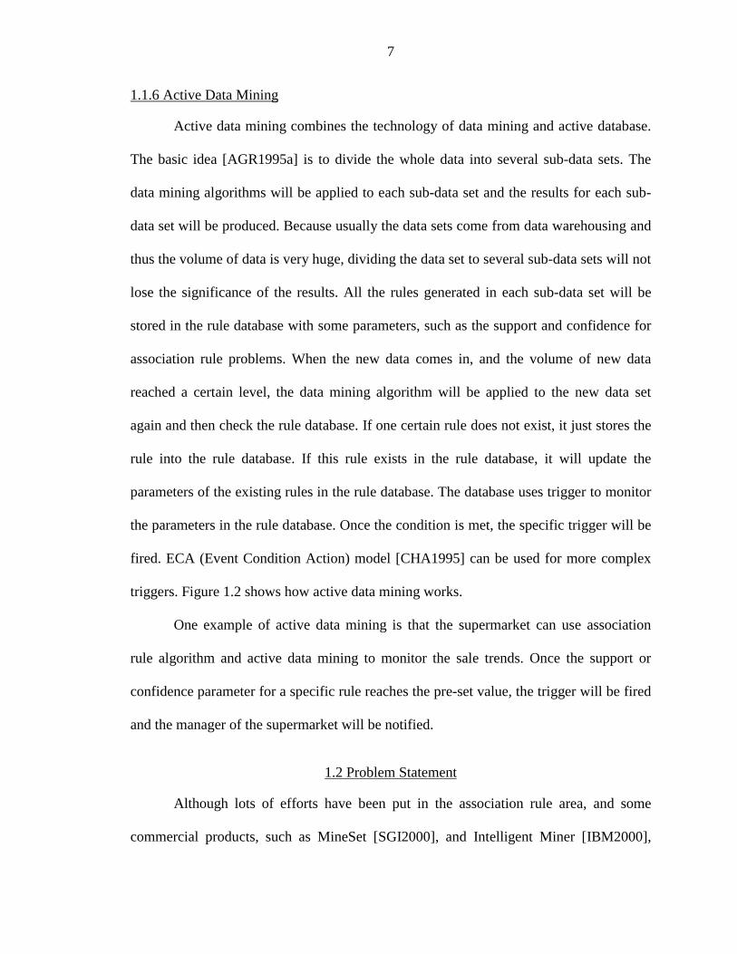
triggers. Figure 1.2 shows how active data mining works.
One example of active data mining is that the supermarket can use association
rule algorithm and active data mining to monitor the sale trends. Once the support or
confidence parameter for a specific rule reaches the pre-set value, the trigger will be fired
and the manager of the supermarket will be notified.
1.2 Problem Statement
Although lots of efforts have been put in the association rule area, and some
commercial products, such as MineSet [SGI2000], and Intelligent Miner [IBM2000],

8
have been developed, there are several limitations in these commercial products. Some of
them are as follows:
Figure 1.2 Active Data Mining
Limitation #1: The first limitation is that the existing software can not connect to
multiple database management systems. These existing commercial products can use the
data from the flat file, or from one specific DBMS as the input data set. For example, the
Intelligent Miner can use the text file or the data stored in DB2 database as the data
source. But in reality, some users may have data stored in multiple database management
systems, so it is very helpful to have the mining software have this ability.
Data mining
Algorithm
Data mining
Algorithm
Data mining
Data mining
Algorithm
Algorithm
UpdateParameters
Large DataSet
Sub-dataset 1
Sub-dataset 2
Sub-dataset n
RuleDatabaseWithparameters
New Data RulesIs the ruleexisting?
N Store the rule
Y
Fire the Trigger
If some parametersmeet the condition
9
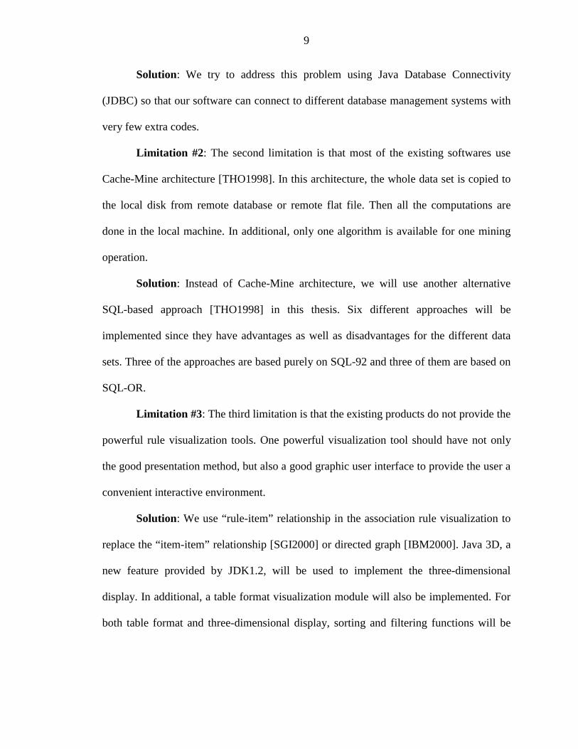
Solution: We try to address this problem using Java Database Connectivity
(JDBC) so that our software can connect to different database management systems with
very few extra codes.
Limitation #2: The second limitation is that most of the existing softwares use
Cache-Mine architecture [THO1998]. In this architecture, the whole data set is copied to
the local disk from remote database or remote flat file. Then all the computations are
done in the local machine. In additional, only one algorithm is available for one mining
operation.
Solution: Instead of Cache-Mine architecture, we will use another alternative
SQL-based approach [THO1998] in this thesis. Six different approaches will be
implemented since they have advantages as well as disadvantages for the different data
sets. Three of the approaches are based purely on SQL-92 and three of them are based on
SQL-OR.
Limitation #3: The third limitation is that the existing products do not provide the
powerful rule visualization tools. One powerful visualization tool should have not only
the good presentation method, but also a good graphic user interface to provide the user a
convenient interactive environment.
Solution: We use “rule-item” relationship in the association rule visualization to
replace the “item-item” relationship [SGI2000] or directed graph [IBM2000]. Java 3D, a
new feature provided by JDK1.2, will be used to implement the three-dimensional
display. In additional, a table format visualization module will also be implemented. For
both table format and three-dimensional display, sorting and filtering functions will be
10
provided through the graphic user interface. It will make our visualization module easier
to use.
Limitation #4: The fourth limitation is also related to the data source. Right now
all the available products can only use the data from one table, but in reality, it is very
common to collect the data from different tables as the input data set. So it is very useful
to have the mining software to have this ability.
Solution: We will provide the user an interface to choose the tables he wants to
use as the data source. For each table, the user can specify the columns that he interests.
Once the system got the information, a set of JOIN/UNION operations will be applied to
generate the suitable input data set.
Limitation #5: The fifth limitation is that in the existing products, all of them use
only one mining algorithm. But in fact some algorithms are better than the other ones for
the different kinds of input data sets. It is useful to have different algorithms available for
different kinds of data sets.
Solution: We plan to implement a Mining Optimizer so that our system will have
the capability to decide which one algorithm should be applied to the particular data set
automatically based on the metadata of the given data set.
In this thesis, we will address the solutions of first three limitations. The solutions
of limitation #4 and #5 are addressed in Mahesh’s thesis [DUD2000].
1.3 Thesis Organization
The remainder of this thesis is organized as follows. In Chapter 2, we describe the
architecture of JDBC, and explain how the JDBC works with different DBMSs. Some
special characteristics of Oracle, such as stored procedure, will also be introduced in that

11
chapter. The six different association rule mining algorithms are presented in Chapter 3.
In Chapter 3, we also provide the performance testing using different kinds of data sets to
verify our analysis of advantage and disadvantage of each mining algorithm.
Visualization of association rules is detailed in Chapter 4. In Chapter 5, we describe the
major parts of the interfaces as well as the architecture of our software. Finally the
conclusions and future work are in Chapter 6.

12
CHAPTER 2ARCHITECTURE AND FEATURES OF JDBC AND ORACLE
In this Chapter, We begin with the introduction of the function of JDBC and the
architecture of JDBC application in Section 2.1. Besides the standard SQL statements, we
also use some additional features provided by the specific DBMS to improve the
performance. Section 2.2 describes these specific features for Oracle.
2.1 JDBC
JDBC (Java Database Connectivity) developed by Sun [SUN2000], is a Java API
for connecting to and executing SQL statements in different Database Management
Systems. JDBC includes a set of classes and interfaces written in Java. They are low-
level APIs, and are used to invoke SQL commands directly. There are two kinds of
models for database access: two-tier and three-tire. In the two-tier model, the client
makes request to a DBMS associated with the server, through JDBC by sending SQL
statements to the server and when the results are ready, the server will send the results
back to the client. In the Three-tier model, instead of sending the request directly to the
database server, the client sends requests to an intermediate server (termed application
server), which applies some business logic, and then the SQL statements are sent to the
database server by the application server. Finally, the result will be returned to the client
through the application server. The advantage of the Three-tier model is that the business
logic can be implemented in the application server, so when the business logic changes,
only the program in the application server needs to be modified accordingly, and it is not
13
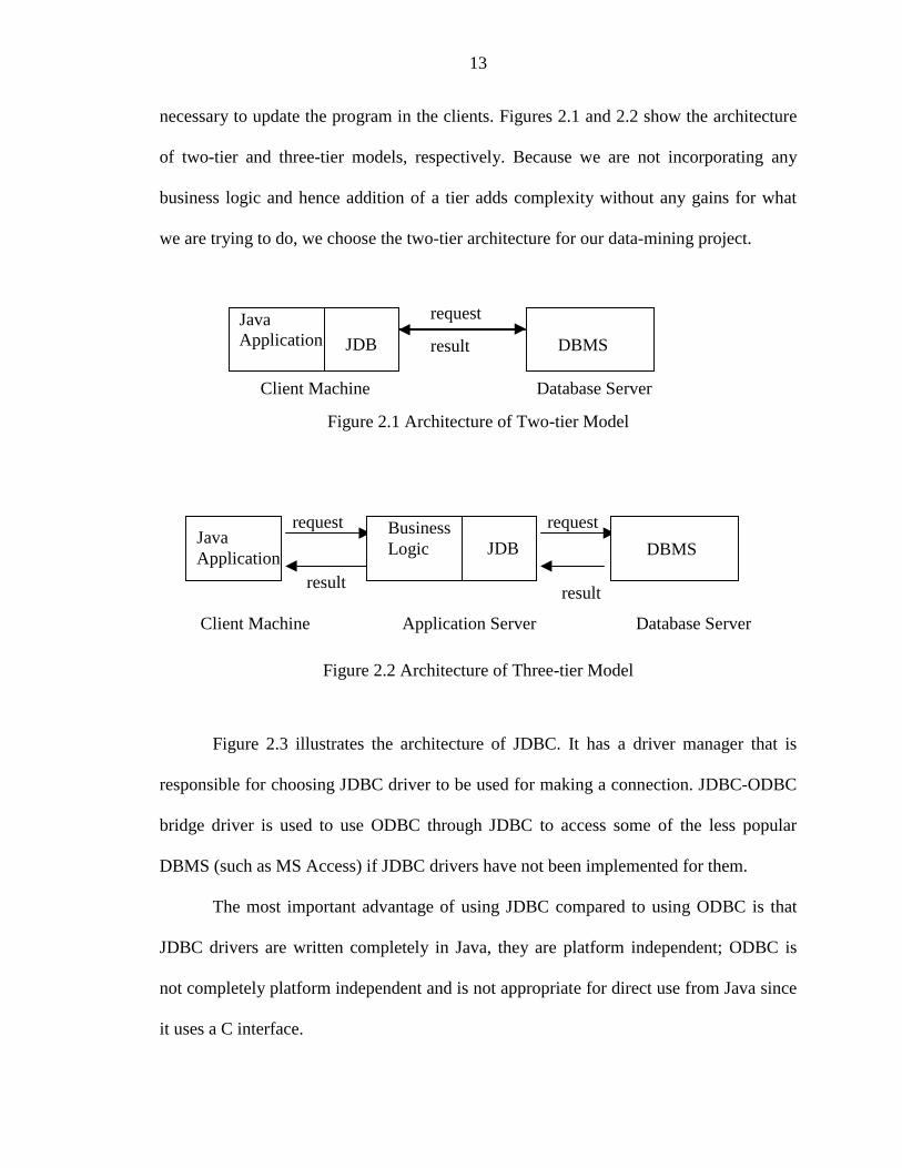
necessary to update the program in the clients. Figures 2.1 and 2.2 show the architecture
of two-tier and three-tier models, respectively. Because we are not incorporating any
business logic and hence addition of a tier adds complexity without any gains for what
we are trying to do, we choose the two-tier architecture for our data-mining project.
Figure 2.1 Architecture of Two-tier Model
Figure 2.2 Architecture of Three-tier Model
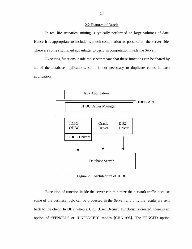
Figure 2.3 illustrates the architecture of JDBC. It has a driver manager that is
responsible for choosing JDBC driver to be used for making a connection. JDBC-ODBC
bridge driver is used to use ODBC through JDBC to access some of the less popular
DBMS (such as MS Access) if JDBC drivers have not been implemented for them.
The most important advantage of using JDBC compared to using ODBC is that
JDBC drivers are written completely in Java, they are platform independent; ODBC is
not completely platform independent and is not appropriate for direct use from Java since
it uses a C interface.
JavaApplication JDB
request
result DBMS
Client Machine Database Server
JavaApplication
request
result
BusinessLogic JDB
request
result
DBMS
Client Machine Database ServerApplication Server
14
2.2 Features of Oracle
In real-life scenarios, mining is typically performed on large volumes of data.
Hence it is appropriate to include as much computation as possible on the server side.
There are some significant advantages to perform computation inside the Server:
Executing functions inside the server means that these functions can be shared by
all of the database applications, so it is not necessary to duplicate codes in each
application.
Figure 2.3 Architecture of JDBC
Execution of function inside the server can minimize the network traffic because
some of the business logic can be processed in the Server, and only the results are sent
back to the client. In DB2, when a UDF (User Defined Function) is created, there is an
option of “FENCED” or ‘UNFENCED” modes [CHA1998]. The FENCED option
Database Server
Java Application
JDBC Driver ManagerJDBC API
JDBC-ODBC
ODBC Drivers
OracleDriver
DB2Driver

15
specifies that the UDF must always be run in an address space that is separate from the
database, while UNFENCED option specifies that the UDF runs in the same address
space as the database. FENCED option causes a performance penalty because of the
process-switching when the UDF is called, but it protects the database integrity against
the accidental damage that might be caused by the function. Oracle does not support this
option.
Oracle provides some mechanisms, such as external procedures, and PL/SQL
procedures to perform computations inside the server. Oracle supports an external
procedure which uses the DLL (Dynamic Link Library) written in the host programming
language such as C. However, Oracle 8.0 does not support the DLL written in Java. If we
used a Java external procedure, we had to use Java Native Interface to communicate
between Java and C programs, as our client is written in Java. This would be inefficient
and increase the implementation effort as well.
PL/SQL stored procedure is another mechanism support by Oracle that meets our
requirements. PL/SQL is a complete, block-structured programming language, and it
provides some additional features that standard SQL does not have, such as loops,
conditional statements, etc. Because the SQL DML (data manipulation language) can be
included inside the PL/SQL stored procedure directly, the results can be saved by
inserting the results into the table. This feature is different from those of DB2. DB2’s
table function does not create a physical table, but in Oracle, a physical table can be
created and values stored in the table. Figure 2.4 illustrates the format of one PL/SQL
stored procedure named ‘SaveTid’. A PL/SQL stored procedure begins with the

16
declaration section followed by the procedure body. The actual code of SaveTid() is
presented and explained in detail in Chapter 3.
Figure 2.4 PL/SQL Stored procedure “SaveTid”
Suppose there is a table TIDITEM.
Table 2.1 TIDITEM Table
Item Tid1 1001 3002 1002 2003 200
The purpose of stored procedure ‘SaveTid’ is to accept one parameter ‘rowcount’
of table TIDITEM. The data of table TIDITEM will be processed row by row. After
processing, the Tid with the same Item will be combined together to form ‘T_Tids’, and
the number of Tid with the same Item will be stored in ‘T_cnt’, and finally, the three
columns ‘T_item’, ‘T_cnt’, and ‘T_tids’ will be inserted into table tidT. The data type
CLOB (Character Large Object) is used for ‘T-tids’ because sometimes the length of
T_tids will exceed the maximum length of VARCHAR2 and CLOB can contain up to
CREATE OR REPLACE PROCEDURE SaveTid(rowCount IN INTEGER) ASDeclaration Section
BEGINRetrieve the data from source table ‘TIDITEM’ one row by one row using
cursor;Processing the data, combine ‘Tid’ for each same ‘Item’;Insert the values into the table ‘tidT’;
END;

17
two gigabytes (231-1 bytes). The ‘INSERT’ statement in the above example will insert the
following values into table tidT as shown in Table 2.2.
Table 2.2 tidT Table
T_item T_cnt T_tids
1 2 100, 3002 2 100, 2003 1 200
If table TIDITEM has millions of rows, and after processing by the stored
procedure, table tidT has only 1,000 rows, the network traffic will be reduced
tremendously since all of the computing work will be done inside the server machine.
18
CHAPTER 3ALTERNATIVE APPROACHES TO ASSOCIATION RULE MINING
In this chapter, we begin with reviewing the related work on association rule
mining algorithms and different architectural alternatives in Section 3.1. The association
rule mining can be broadly divided into two phases: support counting phase and rule
generation phase. In Section 3.2, we present three approaches using pure SQL92 and
another three approaches using stored procedures in Oracle for the support counting
phase. The algorithm for rule generation is presented in Section 3.3. In Section 3.4, we
provided some performance testing using different kinds of data sets for the six
approaches.
3.1 Related Work
3.1.1 Apriori Algorithm
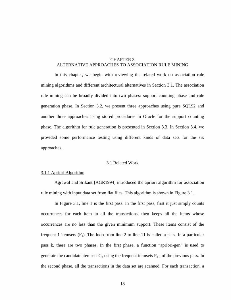
Agrawal and Srikant [AGR1994] introduced the apriori algorithm for association
rule mining with input data set from flat files. This algorithm is shown in Figure 3.1.
In Figure 3.1, line 1 is the first pass. In the first pass, first it just simply counts
occurrences for each item in all the transactions, then keeps all the items whose
occurrences are no less than the given minimum support. These items consist of the
frequent 1-itemsets (F1). The loop from line 2 to line 11 is called a pass. In a particular
pass k, there are two phases. In the first phase, a function “apriori-gen” is used to
generate the candidate itemsets Ck using the frequent itemsets Fk-1 of the previous pass. In
the second phase, all the transactions in the data set are scanned. For each transaction, a
19
function “subset” is called to determine the candidates in Ck that are contained in a given
transaction, then the support of candidates in Ck is counted. At the end of pass k, the
candidate itemsets Ck is examined to determine which of the candidates are frequent.
Those candidates consist of the frequent itemsets Fk of pass k. The loop continues until
Fk-1 is empty, indicating that there is no more frequent itemsets.
The six support counting approaches and rule generation process presented in this
thesis are based on the framework of the above apriori algorithm.
Figure 3.1 Apriori Algorithm
3.1.2 Architectural Alternatives
There are several architectural alternatives for integrating data mining with
relational DBMS [THO1998]. These alternatives include Cache-Mine, SQL-based
approach, and Integrated approach. In this section, we discuss these three architectures.
3.1.2.1 Cache-Mine
Figure 3.2 illustrates the architecture of Cache-Mine approach. In this
architecture, the GUI resides in the client side and the mining kernel can reside in the
1) F1 = {frequent 1-itemsets};2) for ( k=2; Fk-1<>0, k++ ) do begin3) Ck = apriori-gen(Fk-1); // generate new candidate sets4) for all transactions t ∈ D do begin5) Ct = subset(Ck, t); // find all candidate sets contained in t6) for all candidates c ∈ Ct do7) c.count++;8) end9) end10) Fk = {c ∈ Ck | c.count ≥ minsup};11) end12) Answer = ∪ k Fk;

20
client side (2-tier architecture), or in the application server (3-tier architecture). When the
user sends the mining request to the mining kernel, the mining kernel reads data from
DBMS only once and copies the data in flat files on local disk for later use. After the
mining algorithm is executed, the results will be first stored in flat files on local disk, then
sent back to the database server and stored in DBMS. This architecture works very
efficiently because once the data are stored on local disk, the access to the data will be
very fast. One of the disadvantages is that it requires additional disk space to store the
data, especially when the data set is very large.
Figure 3.2 Cache-Mine Architecture
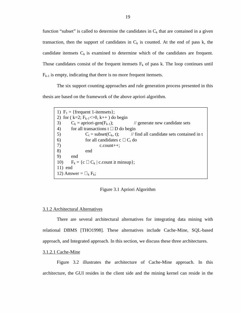
3.1.2.2 SQL-based Approach
The architecture of SQL-based approaches is illustrated in Figure 3.3. When the
user specifies the mining operation, a preprocessor will generate the appropriate SQL
statements for this operation. All the intermediate results are stored in the database. The
SQL statements can be executed on the SQL-92 relational engine, as well as on the newer
object-relational (SQL-OR) engine. SQL-OR provides some more features, such as
CLOB, user-defined function, table function, stored procedure, etc. For this architecture,
all the data and results are stored in the database and the data is never copied into a flat
GUI orMining Language
Mining
Reques
Mining
Kernel
File
DBMS
Data/ Result
DB
21
file on the local disk. This alternative has the following advantages: (1) Additional disk
space is not needed to store the data. (2) The database indexing and query processing
capabilities can be exploited as much as possible. (3) The DBMS check-pointing and
space management can be especially valuable for long-running mining algorithms on
huge volumes of data. (4) SQL-based mining algorithm is very portable if we use only
the standard SQL features. The disadvantage is that it is not as fast as Cache-Mine
alternative because accessing the database generally is slower than accessing a flat file on
the local disk.
Figure 3.3 SQL-based Architecture
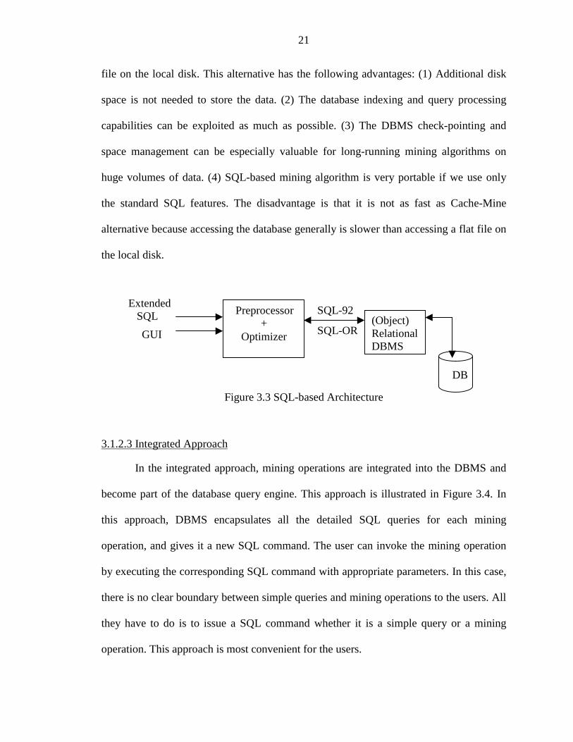
3.1.2.3 Integrated Approach
In the integrated approach, mining operations are integrated into the DBMS and
become part of the database query engine. This approach is illustrated in Figure 3.4. In
this approach, DBMS encapsulates all the detailed SQL queries for each mining
operation, and gives it a new SQL command. The user can invoke the mining operation
by executing the corresponding SQL command with appropriate parameters. In this case,
there is no clear boundary between simple queries and mining operations to the users. All
they have to do is to issue a SQL command whether it is a simple query or a mining
operation. This approach is most convenient for the users.
Extended SQL Preprocessor
+ Optimizer
(Object)RelationalDBMS
DB
GUI
SQL-92
SQL-OR
22
Figure 3.4 Architecture for the Integrated Approach
3.2 Support Counting
For the support counting phase, first we need to generate the candidate sets Ck for
each pass k. Below, we show SQL formulations for candidate set generation.
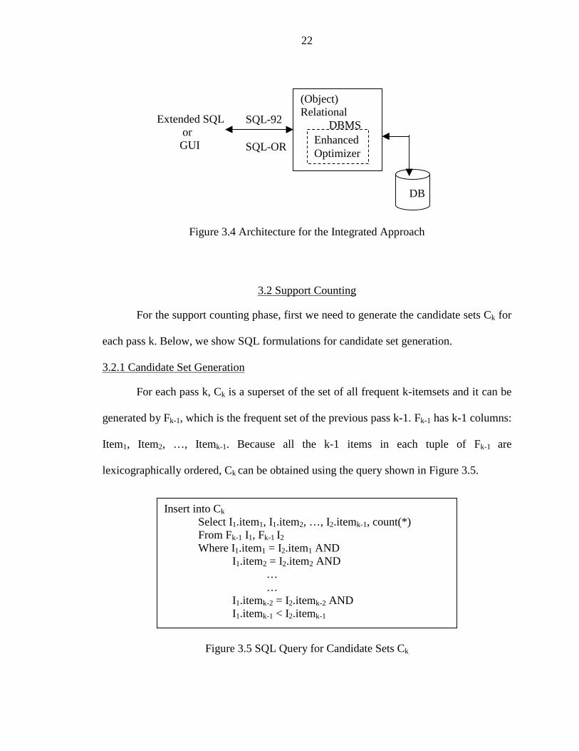
3.2.1 Candidate Set Generation
For each pass k, Ck is a superset of the set of all frequent k-itemsets and it can be
generated by Fk-1, which is the frequent set of the previous pass k-1. Fk-1 has k-1 columns:
Item1, Item2, …, Itemk-1. Because all the k-1 items in each tuple of Fk-1 are
lexicographically ordered, Ck can be obtained using the query shown in Figure 3.5.
Figure 3.5 SQL Query for Candidate Sets Ck
Extended SQL or GUI
(Object)Relational DBMS
DB
SQL-92
SQL-OREnhancedOptimizer
Insert into Ck
Select I1.item1, I1.item2, …, I2.itemk-1, count(*)From Fk-1 I1, Fk-1 I2
Where I1.item1 = I2.item1 ANDI1.item2 = I2.item2 AND
……
I1.itemk-2 = I2.itemk-2 ANDI1.itemk-1 < I2.itemk-1
23
As an illustration, if F3 is {{1, 2, 3}, {1, 2, 4}, {1, 3, 4}, {1, 3, 5}, {2, 3, 4}}, then
the candidate sets of the next pass C4 are {1, 2, 3, 4}, and {1, 3, 4, 5}.
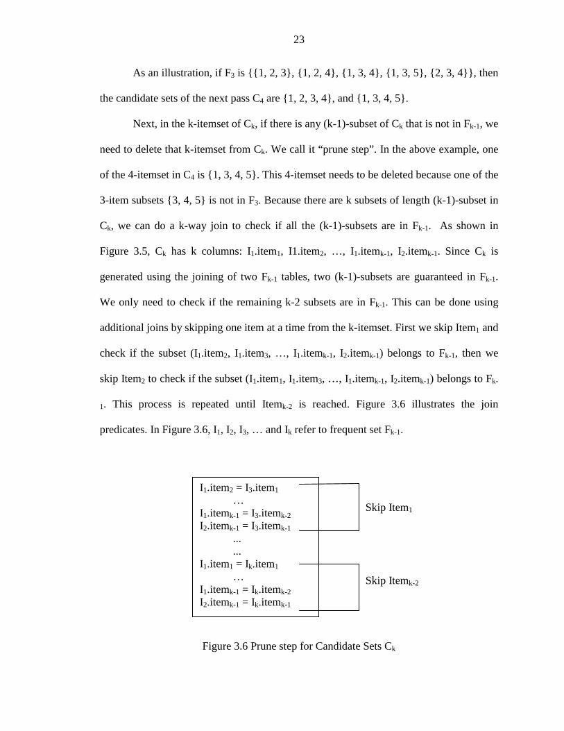
Next, in the k-itemset of Ck, if there is any (k-1)-subset of Ck that is not in Fk-1, we
need to delete that k-itemset from Ck. We call it “prune step”. In the above example, one
of the 4-itemset in C4 is {1, 3, 4, 5}. This 4-itemset needs to be deleted because one of the
3-item subsets {3, 4, 5} is not in F3. Because there are k subsets of length (k-1)-subset in
Ck, we can do a k-way join to check if all the (k-1)-subsets are in Fk-1. As shown in
Figure 3.5, Ck has k columns: I1.item1, I1.item2, …, I1.itemk-1, I2.itemk-1. Since Ck is
generated using the joining of two Fk-1 tables, two (k-1)-subsets are guaranteed in Fk-1.
We only need to check if the remaining k-2 subsets are in Fk-1. This can be done using
additional joins by skipping one item at a time from the k-itemset. First we skip Item1 and
check if the subset (I1.item2, I1.item3, …, I1.itemk-1, I2.itemk-1) belongs to Fk-1, then we
skip Item2 to check if the subset (I1.item1, I1.item3, …, I1.itemk-1, I2.itemk-1) belongs to Fk-
1. This process is repeated until Itemk-2 is reached. Figure 3.6 illustrates the join
predicates. In Figure 3.6, I1, I2, I3, … and Ik refer to frequent set Fk-1.
Figure 3.6 Prune step for Candidate Sets Ck
I1.item2 = I3.item1
…I1.itemk-1 = I3.itemk-2
I2.itemk-1 = I3.itemk-1
...
...I1.item1 = Ik.item1
…I1.itemk-1 = Ik.itemk-2
I2.itemk-1 = Ik.itemk-1
Skip Item1
Skip Itemk-2
24
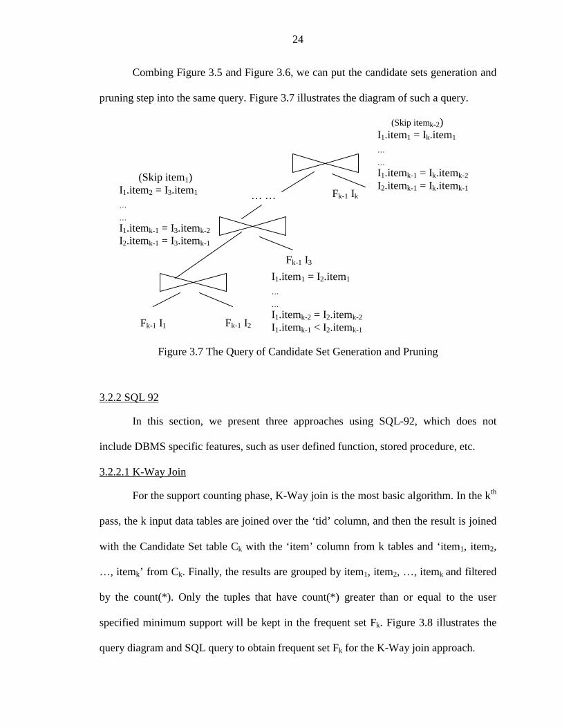
Combing Figure 3.5 and Figure 3.6, we can put the candidate sets generation and
pruning step into the same query. Figure 3.7 illustrates the diagram of such a query.
Figure 3.7 The Query of Candidate Set Generation and Pruning
3.2.2 SQL 92
In this section, we present three approaches using SQL-92, which does not
include DBMS specific features, such as user defined function, stored procedure, etc.
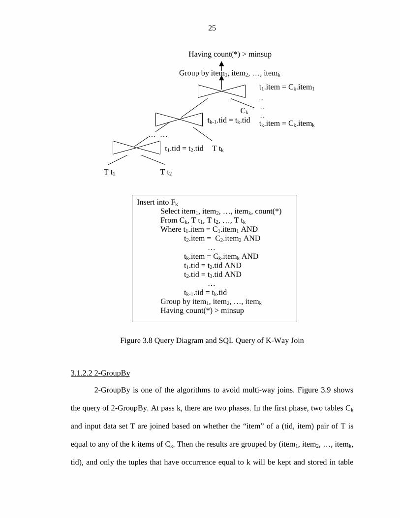
3.2.2.1 K-Way Join
For the support counting phase, K-Way join is the most basic algorithm. In the kth
pass, the k input data tables are joined over the ‘tid’ column, and then the result is joined
with the Candidate Set table Ck with the ‘item’ column from k tables and ‘item1, item2,
…, itemk’ from Ck. Finally, the results are grouped by item1, item2, …, itemk and filtered
by the count(*). Only the tuples that have count(*) greater than or equal to the user
specified minimum support will be kept in the frequent set Fk. Figure 3.8 illustrates the
query diagram and SQL query to obtain frequent set Fk for the K-Way join approach.
Fk-1 I1 Fk-1 I2
Fk-1 I3
… … Fk-1 Ik
I1.item1 = I2.item1
…
…
I1.itemk-2 = I2.itemk-2
I1.itemk-1 < I2.itemk-1
(Skip item1)I1.item2 = I3.item1
…
…
I1.itemk-1 = I3.itemk-2
I2.itemk-1 = I3.itemk-1
(Skip itemk-2)I1.item1 = Ik.item1
…
…
I1.itemk-1 = Ik.itemk-2
I2.itemk-1 = Ik.itemk-1
25
Figure 3.8 Query Diagram and SQL Query of K-Way Join
3.1.2.2 2-GroupBy
2-GroupBy is one of the algorithms to avoid multi-way joins. Figure 3.9 shows
the query of 2-GroupBy. At pass k, there are two phases. In the first phase, two tables Ck
and input data set T are joined based on whether the “item” of a (tid, item) pair of T is
equal to any of the k items of Ck. Then the results are grouped by (item1, item2, …, itemk,
tid), and only the tuples that have occurrence equal to k will be kept and stored in table
T t1 T t2
T tkt1.tid = t2.tid
tk-1.tid = tk.tid
… …
Ck
t1.item = Ck.item1
...
…
…
tk.item = Ck.itemk
Group by item1, item2, …, itemk
Having count(*) > minsup
Insert into Fk
Select item1, item2, …, itemk, count(*)From Ck, T t1, T t2, …, T tk
Where t1.item = C1.item1 ANDt2.item = C2.item2 AND
…tk.item = Ck.itemk ANDt1.tid = t2.tid ANDt2.tid = t3.tid AND
…tk-1.tid = tk.tid
Group by item1, item2, …, itemk
Having count(*) > minsup
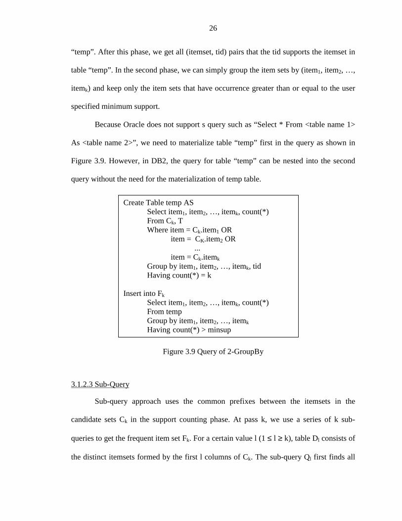
26
“temp”. After this phase, we get all (itemset, tid) pairs that the tid supports the itemset in
table “temp”. In the second phase, we can simply group the item sets by (item1, item2, …,
itemk) and keep only the item sets that have occurrence greater than or equal to the user
specified minimum support.
Because Oracle does not support s query such as “Select * From <table name 1>
As <table name 2>”, we need to materialize table “temp” first in the query as shown in
Figure 3.9. However, in DB2, the query for table “temp” can be nested into the second
query without the need for the materialization of temp table.
Figure 3.9 Query of 2-GroupBy
3.1.2.3 Sub-Query
Sub-query approach uses the common prefixes between the itemsets in the
candidate sets Ck in the support counting phase. At pass k, we use a series of k sub-
queries to get the frequent item set Fk. For a certain value l (1 ≤ l ≥ k), table Dl consists of
the distinct itemsets formed by the first l columns of Ck. The sub-query Ql first finds all
Create Table temp ASSelect item1, item2, …, itemk, count(*)From Ck, TWhere item = Ck.item1 OR
item = CK.item2 OR...
item = Ck.itemk
Group by item1, item2, …, itemk, tidHaving count(*) = k
Insert into Fk
Select item1, item2, …, itemk, count(*)From tempGroup by item1, item2, …, itemk
Having count(*) > minsup

27
tids that match the distinct itemsets of Dl. Then the result is joined with the input data
table T and table Dl+1 to get Ql+1. Finally, the frequent item set Fk can be get by grouping
Qk and only keep the tuples that have their occurrence greater than or equal to the user
specified minimum support. Figure 3.10 illustrates the SQL query and query diagram of
this approach.
Figure 3.10 Query Diagram and SQL Query of Sub-Query
Rl-1.iteml = Dl.iteml
…
Rl-1.iteml-1 = Dl.iteml-1
T tl
item1, item2, …., iteml, tid
Subquery Ql
Subquery Ql-Select distinctitem1, …, iteml from Ck
Rl-1Dl
tl.item = Dl.iteml
Insert into Fk
Select item1, item2, …, itemk, count(*)From (Subquery Qk) tGroup by item1, item2, …, itemk
Having count(*) > minsup
Subquery Ql (for any l between 1 and k)Select item1, item2, …, iteml, tidFrom T tl, (Subquery Ql-1) as Rl-1,
(Select distinct item1, item2, …, iteml From Ck) as Dl
Where Rl-1.item1 = Dl.item1 AND …
Rl-1.iteml-1 = Dl.iteml-1 ANDRl-1.tid = tl.tid ANDtl.item = Dl.iteml
Subquery Q0: No subquery Q0

28
3.2.3 SQL-OR
Besides the standard SQL, each DBMS has some particular features that extend
the ability of standard SQL. For example, DB2 allows the user to create “User Defined
Function” (UDF) using a (host) programming language. The UDF is registered with the
server and executed either within or outside the server address space (unfenced and
fenced, respectively). The unfenced mode executes more efficiently than runs on the
client side in the Client/Server computing environment. In Oracle, the user can define
“Stored Procedure,” which uses PL/SQL (Oracle’s procedural extensions to SQL), as the
programming language. The advantages of using stored procedure in Oracle have been
listed in Chapter 2. In this section, we present three approaches using stored procedure.
For DB2, we use the UDF feature for the following three approaches. The algorithms that
use UDF in DB2 are presented in Mahesh’s thesis [DUD2000]. The major difference of
DB2 UDF and Oracle Stored procedure is that UDF uses a host programming language,
while Oracle Stored procedure uses PL/SQL.
In stored procedure, the table names that are used in the stored procedure should
exist when the stored procedure is compiled because Oracle checks the syntax during
compiling. So we can not pass the table name as a parameter to the stored procedure.
Because of this reason, we reserve “TIDITEM” as the input table name. Each time,
before applying the mining algorithm, we rename the input table to “TIDITEM”, then
table “TIDITEM” is renamed back to the original name after the mining algorithm is
finished.
3.2.3.1 Vertical
In the vertical approach, first we transfer the input data into a vertical form by
creating a table “TIDT” which has three columns: ITEM, CNT and TIDS. ITEM is the
29
distinct item from all transactions, TIDS contains all the tids that associated with this
particular item, and CNT is the number of tid for a particular item. For the sample data
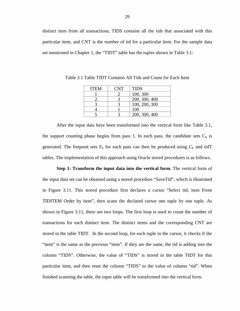
set mentioned in Chapter 1, the “TIDT” table has the tuples shown in Table 3.1:
Table 3.1 Table TIDT Contains All Tids and Count for Each Item
ITEM CNT TIDS1 2 100, 3002 3 200, 300, 4003 3 100, 200, 3004 1 1005 3 200, 300, 400
After the input data have been transformed into the vertical form like Table 3.1,
the support counting phase begins from pass 1. In each pass, the candidate sets Ck is
generated. The frequent sets Fk for each pass can then be produced using Ck and tidT
tables. The implementation of this approach using Oracle stored procedures is as follows.
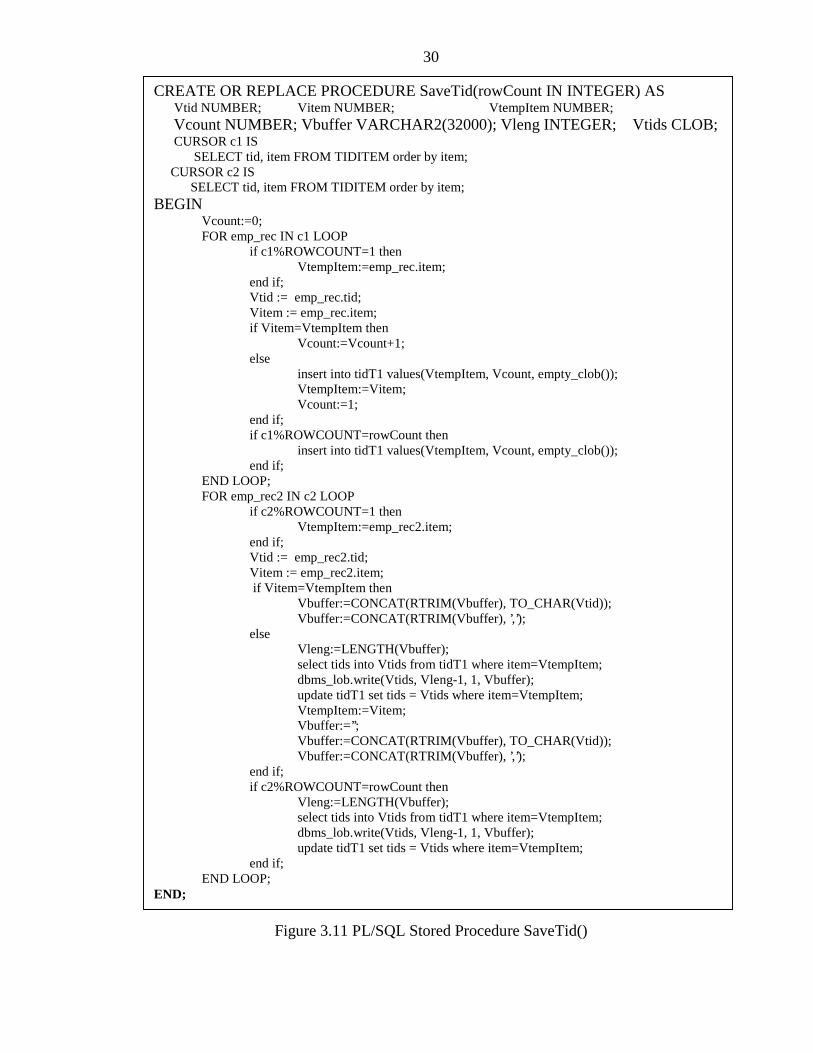
Step 1: Transform the input data into the vertical form. The vertical form of
the input data set can be obtained using a stored procedure “SaveTid”, which is illustrated
in Figure 3.11. This stored procedure first declares a cursor “Select tid, item From
TIDITEM Order by item”, then scans the declared cursor one tuple by one tuple. As
shown in Figure 3.11, there are two loops. The first loop is used to count the number of
transactions for each distinct item. The distinct items and the corresponding CNT are
stored in the table TIDT. In the second loop, for each tuple in the cursor, it checks if the
“item” is the same as the previous “item”. If they are the same, the tid is adding into the
column “TIDS”. Otherwise, the value of “TIDS” is stored in the table TIDT for this
particular item, and then reset the column “TIDS” to the value of column “tid”. When
finished scanning the table, the input table will be transformed into the vertical form.
30
Figure 3.11 PL/SQL Stored Procedure SaveTid()
CREATE OR REPLACE PROCEDURE SaveTid(rowCount IN INTEGER) AS Vtid NUMBER; Vitem NUMBER; VtempItem NUMBER; Vcount NUMBER; Vbuffer VARCHAR2(32000); Vleng INTEGER; Vtids CLOB; CURSOR c1 IS SELECT tid, item FROM TIDITEM order by item; CURSOR c2 IS SELECT tid, item FROM TIDITEM order by item;BEGIN
Vcount:=0;FOR emp_rec IN c1 LOOP
if c1%ROWCOUNT=1 thenVtempItem:=emp_rec.item;
end if;Vtid := emp_rec.tid;Vitem := emp_rec.item;if Vitem=VtempItem then
Vcount:=Vcount+1;else
insert into tidT1 values(VtempItem, Vcount, empty_clob());VtempItem:=Vitem;Vcount:=1;
end if;if c1%ROWCOUNT=rowCount then
insert into tidT1 values(VtempItem, Vcount, empty_clob());end if;
END LOOP;FOR emp_rec2 IN c2 LOOP
if c2%ROWCOUNT=1 thenVtempItem:=emp_rec2.item;
end if;Vtid := emp_rec2.tid;Vitem := emp_rec2.item;
if Vitem=VtempItem thenVbuffer:=CONCAT(RTRIM(Vbuffer), TO_CHAR(Vtid));Vbuffer:=CONCAT(RTRIM(Vbuffer), ’,’);
elseVleng:=LENGTH(Vbuffer);select tids into Vtids from tidT1 where item=VtempItem;dbms_lob.write(Vtids, Vleng-1, 1, Vbuffer);update tidT1 set tids = Vtids where item=VtempItem;VtempItem:=Vitem;Vbuffer:=’’;Vbuffer:=CONCAT(RTRIM(Vbuffer), TO_CHAR(Vtid));Vbuffer:=CONCAT(RTRIM(Vbuffer), ’,’);
end if;if c2%ROWCOUNT=rowCount then
Vleng:=LENGTH(Vbuffer);select tids into Vtids from tidT1 where item=VtempItem;dbms_lob.write(Vtids, Vleng-1, 1, Vbuffer);update tidT1 set tids = Vtids where item=VtempItem;
end if;END LOOP;
END;
31
Step 2: Get the frequent set F1 in pass 1. Because we already have the table
TIDT, which contains the columns ITEM, CNT, and TIDS, it is very easy to get the
frequent set F1. We can just keep the ITEM where CNT is greater than or equal to the
given minimum support. This can be done using a query “Insert into F1 select ITEM,
CNT from TIDT Where CNT>=:minsupport”.
Step 3: In pass k (k>=2), get the candidate set Ck. Table Ck has k columns
item1, item2, …, itemk. It can be obtained using the method described in Section 3.1
Step 4: In pass k (k>=2), get the frequent set Fk. For the support counting, we
need to get the occurrence of each tuple in Ck. After we have the table “TIDT”, we can
obtain the occurrence of “item1, item2, …, itemk” by counting the number of tids in the
intersection of these items. In this example (Table 3.1), for the item set “2, 3”, the
common tids of the items “2” and “3” are “200”, and “300”, so the number of common
tids is 2. Therefore, the support of item set “2, 3” is 2. We created a series of stored
procedures “CountAndk” for this task. The stored procedure “CountAndk” takes k
parameters (each parameter is a tid-list), and return the number of common tids among
these k tids. . Figure 3.12 illustrates the stored procedure “CountAnd2”. “CountAnd2”
first read the two tid-lists into two arrays, then the number of common tids among these
two tid-lists can be obtained by scanning these two arrays. We can apply the stored
procedure “CountAndk” for each tuple in Ck to get the number of common tid for each
item set. The item sets Ck can be expanded to the frequent sets Fk by adding the support
count for each tuple into the table Ck and then delete the tuples whose support count is
less than the user specified minimum support.

32
Figure 3.12 Stored Procedure CountAnd2()
CREATE OR REPLACE FUNCTION countAnd2(in1 CLOB, in2 CLOB) RETURN NUMBER IS returnCountNUMBER;
TYPE vType IS VARRAY(10000) OF VARCHAR2(50); v1 vType; v2 vType; pos1 INTEGER; pos2 INTEGER; item VARCHAR2(20); curChar CHAR(1); patt VARCHAR2(10); len INTEGER; clob1Len INTEGER; clob2Len INTEGER; loopCount INTEGER; lastItem INTEGER;BEGIN returnCount:=0;-- initialize the varrays v1:=vType(NULL); v2:=vType(NULL); patt:=’,’; -- pattern i s ’,’ clob1Len := DBMS_LOB.GETLENGTH(in1); --get the clob1 length item:=’’; loopCount:=0;-- dbms_output.put_line(’Varray 1’); FOR i IN 1..clob1Len LOOP curChar:=DBMS_LOB.SUBSTR(in1,1,i); IF curChar=patt THEN
loopCount:=loopCount+1;v1(loopCount):=item;v1.extend;item:=’’;
-- dbms_output.put_line(’v1(’ ||loopCount|| ’) : ’ || v1(loopCount)); ELSE
item:=item || curChar; END IF; END LOOP; loopCount:=loopCount+1; v1(loopCount):=item;-- dbms_output.put_line(’v1(’ ||loopCount|| ’) : ’ || v1(loopCount));-----------Till here for VARRAY v1 clob2Len := DBMS_LOB.GETLENGTH(in2); --get the clob1 length item:=’’; loopCount:=0;-- dbms_output.put_line(’Varray 2’); FOR i IN 1..clob2Len LOOP curChar:=DBMS_LOB.SUBSTR(in2,1,i); IF curChar=patt THEN
loopCount:=loopCount+1;v2(loopCount):=item;v2.extend;item:=’’;
-- dbms_output.put_line(’v2(’ ||loopCount|| ’) : ’ || v2(loopCount)); ELSE
item:=item || curChar; END IF; END LOOP; loopCount:=loopCount+1; v2(loopCount):=item;-- dbms_output.put_line(’v2(’ ||loopCount|| ’) : ’ || v2(loopCount));-----------Till here for VARRAY v2-- now have to loop till the end of the arrays and meanwhile count the common items. clob1Len := v1.COUNT; clob2Len := v2.COUNT; FOR i IN 1..clob1Len LOOP
FOR j IN 1..clob2Len LOOPIF v1(i)=v2(j) THEN
returnCount:=returnCount+1;END IF;
END LOOP; END LOOP; return (returnCount);END;

33
3.2.3.2 GatherJoin
The GathoerJoin approach first transer the input data into a vertical form by
creating a table “TITEM” which has three columns: TID, CNT and ITEMS. TID contains
the distinct tids in all transactions. ITEMS contain all the items that belong to a particular
tid. CNT is the number of items for the particular tid. The table TIETM created from the
example input data set is shown in Table 3.2.
Table 3.2 Table TITEM Contains All Items and Count for each Tid
TID CNT ITEMS100 3 1, 3, 4200 3 2, 3, 5300 4 1, 2, 3, 5400 2 2, 5
After the input data has been transformed into the vertical form like Table 3.2, the
support counting phase begins from pass 1. In each pass, the candidate sets Ck is not
needed because we already have the table TITEM. The frequent item sets Fk can be
produced based purely on table TITEM. The implementation of this approach using
Oracle stored procedures is as follows.
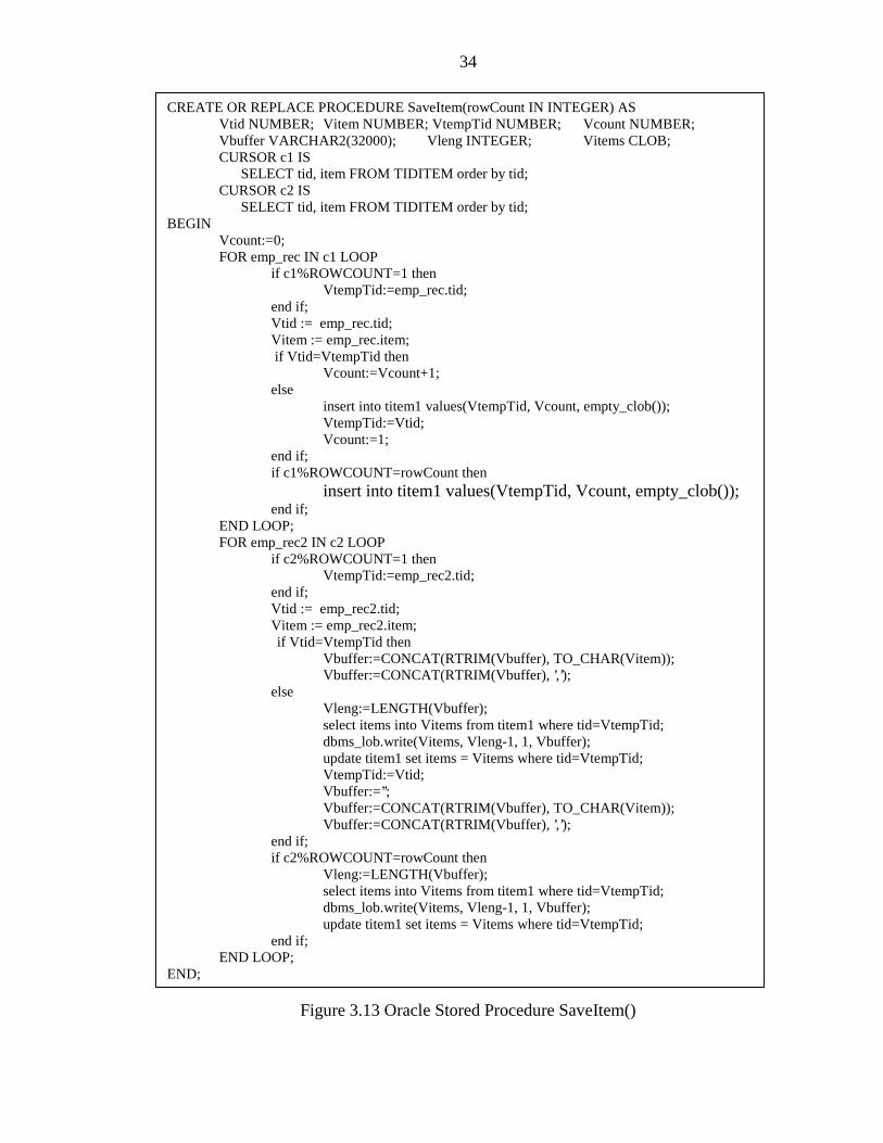
Step 1: Transform the input data into the vertical form. The vertical form of
the input data set can be obtained using a stored procedure “SaveItem”, which is shown
in Figure 3.13. This stored procedure first declares a cursor “Select tid, item From
TIDITEM Order by tid”, then scans the declared cursor one tuple by one tuple. As shown
in Figure 3.13, there are two loops. The first loop is used to count the number of items for
each distinct transaction. The distinct transactions and the corresponding CNT are stored
in the table TITEM.
34
Figure 3.13 Oracle Stored Procedure SaveItem()
CREATE OR REPLACE PROCEDURE SaveItem(rowCount IN INTEGER) ASVtid NUMBER; Vitem NUMBER; VtempTid NUMBER; Vcount NUMBER;Vbuffer VARCHAR2(32000); Vleng INTEGER; Vitems CLOB;CURSOR c1 IS SELECT tid, item FROM TIDITEM order by tid;CURSOR c2 IS SELECT tid, item FROM TIDITEM order by tid;
BEGIN Vcount:=0;
FOR emp_rec IN c1 LOOPif c1%ROWCOUNT=1 then
VtempTid:=emp_rec.tid;end if;Vtid := emp_rec.tid;Vitem := emp_rec.item;
if Vtid=VtempTid thenVcount:=Vcount+1;
elseinsert into titem1 values(VtempTid, Vcount, empty_clob());VtempTid:=Vtid;Vcount:=1;
end if;if c1%ROWCOUNT=rowCount then
insert into titem1 values(VtempTid, Vcount, empty_clob());end if;
END LOOP;FOR emp_rec2 IN c2 LOOP
if c2%ROWCOUNT=1 thenVtempTid:=emp_rec2.tid;
end if;Vtid := emp_rec2.tid;Vitem := emp_rec2.item;
if Vtid=VtempTid thenVbuffer:=CONCAT(RTRIM(Vbuffer), TO_CHAR(Vitem));Vbuffer:=CONCAT(RTRIM(Vbuffer), ’,’);
elseVleng:=LENGTH(Vbuffer);select items into Vitems from titem1 where tid=VtempTid;dbms_lob.write(Vitems, Vleng-1, 1, Vbuffer);update titem1 set items = Vitems where tid=VtempTid;VtempTid:=Vtid;Vbuffer:=’’;Vbuffer:=CONCAT(RTRIM(Vbuffer), TO_CHAR(Vitem));Vbuffer:=CONCAT(RTRIM(Vbuffer), ’,’);
end if;if c2%ROWCOUNT=rowCount then
Vleng:=LENGTH(Vbuffer);select items into Vitems from titem1 where tid=VtempTid;dbms_lob.write(Vitems, Vleng-1, 1, Vbuffer);update titem1 set items = Vitems where tid=VtempTid;
end if;END LOOP;
END;

35
In the second loop, for each tuple in the cursor, it checks if the “tid” is the same as
the previous “tid”. If they are the same, the item is adding into the column “ITEMS”.
Otherwise, the value of “ITEMS” is stored in the table TITEM for this particular tid, and
then reset the column “ITEMS” to the value of column “item”. When finished scanning
the table, the input table will be transformed into the vertical form.
Step 2: Get the frequent set F1 in pass 1. The frequent set F1 can be obtained by
querying the input table TIDITEM. We just keep the items that the occurrence is greater
than or equal to the given minimum support. The query “Insert into F1 Select item,
count(*) from TIDITEM Group by item Having count(*)>=:minsupport” should do it.
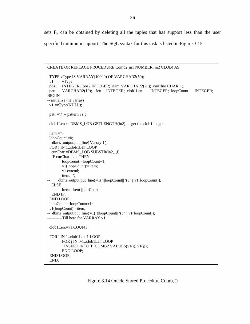
Step 3: In pass k (k>=2), get the frequent set Fk. Once we got the TITEM table,
we have stored all the items which has the same tid into one column (ITEMS). For the
support counting in pass k, we have a series of stored procedures “Combk” to find all the
k-item combinations of items in the column ITEMS. For example, for the third row of
Table 3.2 (TID=300), at pass 3, the stored procedure “Comb3” generates the following
combinations: {1,2,3}, {1,2,5}, {1,3,5}, and {2,3,5}. Figure 3.14 shows stored procedure
“Comb2”, which takes one parameter (item-list) and generates all the 2-item
combinations of items in the column ITEMS. As shown in Figure 3.14, it first reads the
item-list into an array, and then the 2-item combinations of items can be obtained by
scanning the array. In pass k, each tuple of table TITEM is processed using the stored
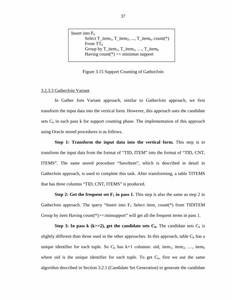
procedure “Combk” and the generated k-item combinations are stored in a table TTk
which has k columns: T_item1, T_item2, …, T_itemk. Finally, the support of each k-item
combination can be obtained easily by using the “Group By” query and the frequent item
36
sets Fk can be obtained by deleting all the tuples that has support less than the user
specified minimum support. The SQL syntax for this task is listed in Figure 3.15.
Figure 3.14 Oracle Stored Procedure Comb2()
CREATE OR REPLACE PROCEDURE Comb2(in1 NUMBER, in2 CLOB) AS
TYPE vType IS VARRAY(10000) OF VARCHAR2(50); v1 vType; pos1 INTEGER; pos2 INTEGER; item VARCHAR2(20); curChar CHAR(1); patt VARCHAR2(10); len INTEGER; clob1Len INTEGER; loopCount INTEGER;BEGIN-- initialize the varrays v1:=vType(NULL);
patt:=’,’; -- pattern i s ’,’
clob1Len := DBMS_LOB.GETLENGTH(in2); --get the clob1 length
item:=’’; loopCount:=0;-- dbms_output.put_line(’Varray 1’); FOR i IN 1..clob1Len LOOP curChar:=DBMS_LOB.SUBSTR(in2,1,i); IF curChar=patt THEN
loopCount:=loopCount+1;v1(loopCount):=item;v1.extend;item:=’’;
-- dbms_output.put_line(’v1(’ ||loopCount|| ’) : ’ || v1(loopCount)); ELSE
item:=item || curChar; END IF; END LOOP; loopCount:=loopCount+1; v1(loopCount):=item;-- dbms_output.put_line(’v1(’ ||loopCount|| ’) : ’ || v1(loopCount));-----------Till here for VARRAY v1
clob1Len:=v1.COUNT;
FOR i IN 1..clob1Len-1 LOOPFOR j IN i+1..clob1Len LOOP INSERT INTO T_COMB2 VALUES(v1(i), v1(j));END LOOP;
END LOOP; END;
37
Figure 3.15 Support Counting of GathorJoin
3.2.3.3 GatherJoin Variant
In Gather Join Variant approach, similar to GatherJoin approach, we first
transform the input data into the vertical form. However, this approach uses the candidate
sets Ck in each pass k for support counting phase. The implementation of this approach
using Oracle stored procedures is as follows.
Step 1: Transform the input data into the vertical form. This step is to
transform the input data from the format of “TID, ITEM” into the format of “TID, CNT,
ITEMS”. The same stored procedure “SaveItem”, which is described in detail in
GatherJoin approach, is used to complete this task. After transforming, a table TITEMS
that has three columns “TID, CNT, ITEMS” is produced.
Step 2: Get the frequent set F1 in pass 1. This step is also the same as step 2 in
GatherJoin approach. The query “Insert into F1 Select item, count(*) from TIDITEM
Group by item Having count(*)>=:minsupport” will get all the frequent items in pass 1.
Step 3: In pass k (k>=2), get the candidate sets Ck. The candidate sets Ck is
slightly different than those used in the other approaches. In this approach, table Ck has a
unique identifier for each tuple. So Ck has k+1 columns: oid, item1, item2, …, itemk
where oid is the unique identifier for each tuple. To get Ck, first we use the same
algorithm described in Section 3.2.1 (Candidate Set Generation) to generate the candidate
Insert into Fk
Select T_item1, T_item2, ..., T_itemk, count(*)From TTk
Group by T_item1, T_item2, …, T_itemk
Having count(*) >= minimun support
38
sets, then we use the stored procedure “CreateCk” to add one column “oid” into the
candidate sets. “oid” will be filled with the unique number begin with 1.
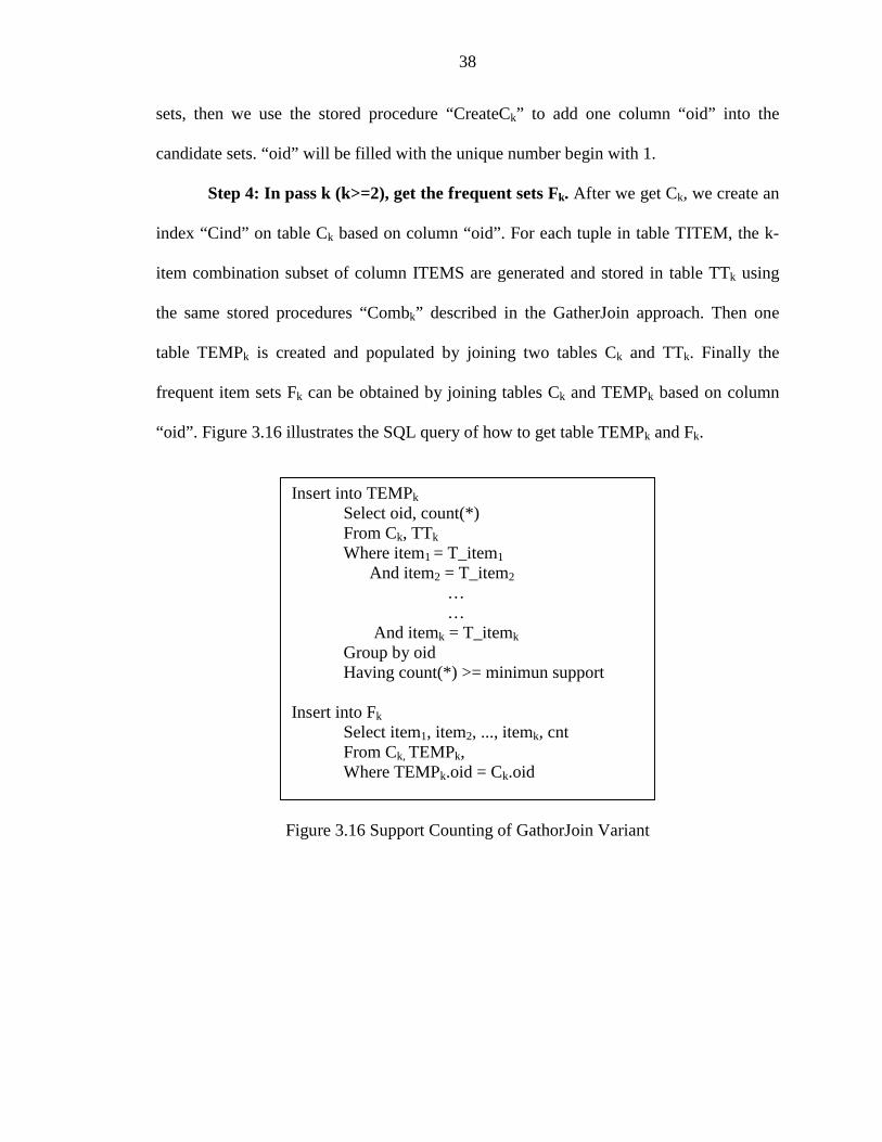
Step 4: In pass k (k>=2), get the frequent sets Fk. After we get Ck, we create an
index “Cind” on table Ck based on column “oid”. For each tuple in table TITEM, the k-
item combination subset of column ITEMS are generated and stored in table TTk using
the same stored procedures “Combk” described in the GatherJoin approach. Then one
table TEMPk is created and populated by joining two tables Ck and TTk. Finally the
frequent item sets Fk can be obtained by joining tables Ck and TEMPk based on column
“oid”. Figure 3.16 illustrates the SQL query of how to get table TEMPk and Fk.
Figure 3.16 Support Counting of GathorJoin Variant
Insert into TEMPk
Select oid, count(*)From Ck, TTk
Where item1 = T_item1
And item2 = T_item2
……
And itemk = T_itemk
Group by oidHaving count(*) >= minimun support
Insert into Fk
Select item1, item2, ..., itemk, cntFrom Ck, TEMPk,Where TEMPk.oid = Ck.oid
39
3.3 Rule Generation
3.3.1 Intermediate Rule Generation
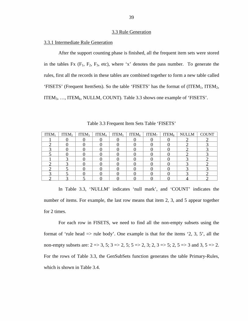
After the support counting phase is finished, all the frequent item sets were stored
in the tables Fx (F1, F2, F3, etc), where ‘x’ denotes the pass number. To generate the
rules, first all the records in these tables are combined together to form a new table called
‘FISETS’ (Frequent ItemSets). So the table ‘FISETS’ has the format of (ITEM1, ITEM2,
ITEM3, …, ITEMk, NULLM, COUNT). Table 3.3 shows one example of ‘FISETS’.
Table 3.3 Frequent Item Sets Table ‘FISETS’
ITEM1 ITEM2 ITEM3 ITEM4 ITEM5 ITEM6 ITEM7 ITEM8 NULLM COUNT1 0 0 0 0 0 0 0 2 22 0 0 0 0 0 0 0 2 33 0 0 0 0 0 0 0 2 35 0 0 0 0 0 0 0 2 31 3 0 0 0 0 0 0 3 22 3 0 0 0 0 0 0 3 22 5 0 0 0 0 0 0 3 33 5 0 0 0 0 0 0 3 22 3 5 0 0 0 0 0 4 2
In Table 3.3, ‘NULLM’ indicates ‘null mark’, and ‘COUNT’ indicates the
number of items. For example, the last row means that item 2, 3, and 5 appear together
for 2 times.
For each row in FISETS, we need to find all the non-empty subsets using the
format of ‘rule head => rule body’. One example is that for the items ‘2, 3, 5’, all the
non-empty subsets are: 2 => 3, 5; 3 => 2, 5; 5 => 2, 3; 2, 3 => 5; 2, 5 => 3 and 3, 5 => 2.
For the rows of Table 3.3, the GenSubSets function generates the table Primary-Rules,
which is shown in Table 3.4.
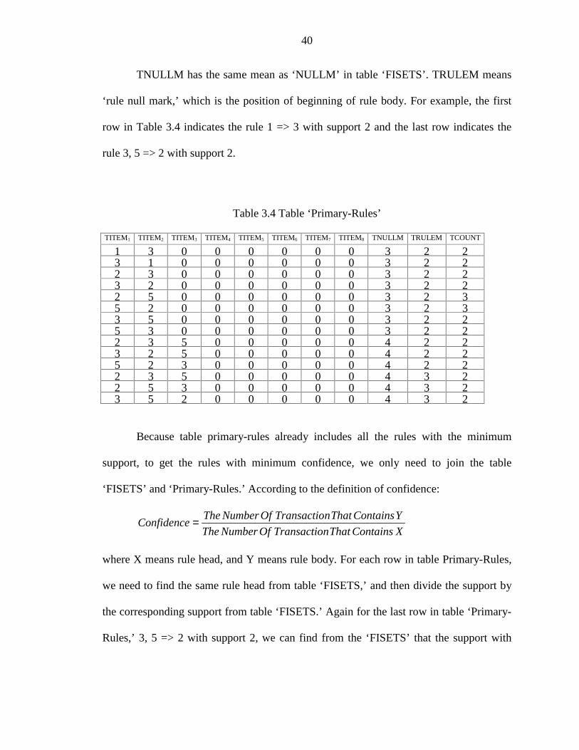
40
TNULLM has the same mean as ‘NULLM’ in table ‘FISETS’. TRULEM means
‘rule null mark,’ which is the position of beginning of rule body. For example, the first
row in Table 3.4 indicates the rule 1 => 3 with support 2 and the last row indicates the
rule 3, 5 => 2 with support 2.
Table 3.4 Table ‘Primary-Rules’
TITEM1 TITEM2 TITEM3 TITEM4 TITEM5 TITEM6 TITEM7 TITEM8 TNULLM TRULEM TCOUNT
1 3 0 0 0 0 0 0 3 2 23 1 0 0 0 0 0 0 3 2 22 3 0 0 0 0 0 0 3 2 23 2 0 0 0 0 0 0 3 2 22 5 0 0 0 0 0 0 3 2 35 2 0 0 0 0 0 0 3 2 33 5 0 0 0 0 0 0 3 2 25 3 0 0 0 0 0 0 3 2 22 3 5 0 0 0 0 0 4 2 23 2 5 0 0 0 0 0 4 2 25 2 3 0 0 0 0 0 4 2 22 3 5 0 0 0 0 0 4 3 22 5 3 0 0 0 0 0 4 3 23 5 2 0 0 0 0 0 4 3 2
Because table primary-rules already includes all the rules with the minimum
support, to get the rules with minimum confidence, we only need to join the table
‘FISETS’ and ‘Primary-Rules.’ According to the definition of confidence:
XContainsThatnTransactioOfNumberThe
YContainsThatnTransactioOfNumberTheConfidence =
where X means rule head, and Y means rule body. For each row in table Primary-Rules,
we need to find the same rule head from table ‘FISETS,’ and then divide the support by
the corresponding support from table ‘FISETS.’ Again for the last row in table ‘Primary-
Rules,’ 3, 5 => 2 with support 2, we can find from the ‘FISETS’ that the support with

41
item ‘3, 5’ is 2, so the confidence of rule ‘3, 5 => 2’ is 2/2=100%. Figure 3.17 is the join
query to accomplish this task.
Figure 3.17 Association Rules Generation Query
Table 3.5 shows all the rules that has the confidence >=50%.
Table 3.5 Table ‘Rules’
ITEM1 ITEM2 ITEM3 ITEM4 ITEM5 ITEM6 ITEM7 ITEM8 NULLM RULEM CONF SUP
1 3 0 0 0 0 0 0 3 2 100 503 1 0 0 0 0 0 0 3 2 66.67 502 3 0 0 0 0 0 0 3 2 66.67 503 2 0 0 0 0 0 0 3 2 66.67 502 5 0 0 0 0 0 0 3 2 100 755 2 0 0 0 0 0 0 3 2 100 753 5 0 0 0 0 0 0 3 2 66.67 505 3 0 0 0 0 0 0 3 2 66.67 502 3 5 0 0 0 0 0 4 2 66.67 503 2 5 0 0 0 0 0 4 2 66.67 505 2 3 0 0 0 0 0 4 2 66.67 502 3 5 0 0 0 0 0 4 3 100 502 5 3 0 0 0 0 0 4 3 66.67 503 5 2 0 0 0 0 0 4 3 100 50
Insert into RulesSelect TITEM1, TITEM2, …, TITEMk, TNULLM, TRULEM,
TCOUNT, (TCOUNT/COUNT)*100From Primary-Rules t1, FISETS t2Where (t1.titem1 = t2.item2 or t1.TRULEM<=1) AND
(t1.titem2 = t2.item3 or t1.TRULEM<=2) AND…
(t1.titemk= t2.itemk or t1.TRULEM<=k) AND t1.TRULEM = t2.NULLM AND(TCOUNT/COUNT)*100 >= min confidence
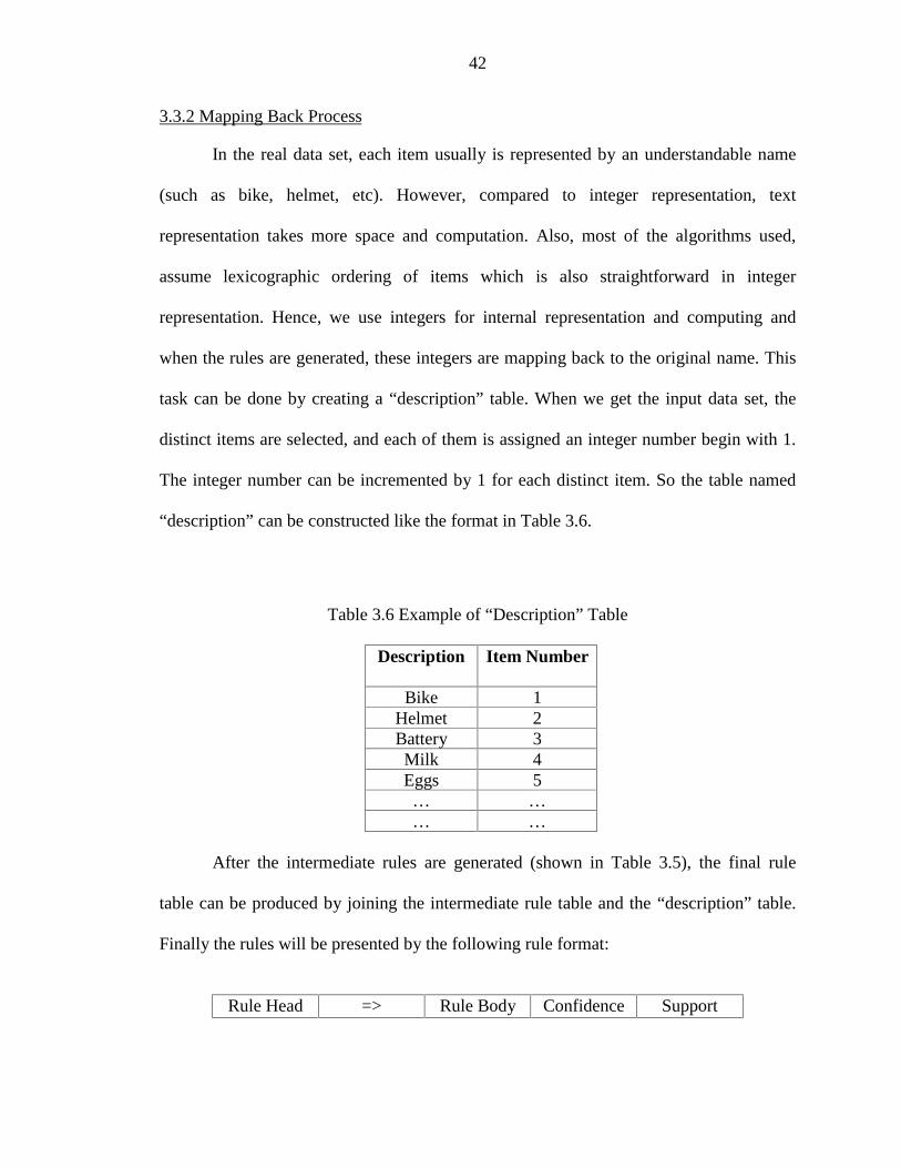
42
3.3.2 Mapping Back Process
In the real data set, each item usually is represented by an understandable name
(such as bike, helmet, etc). However, compared to integer representation, text
representation takes more space and computation. Also, most of the algorithms used,
assume lexicographic ordering of items which is also straightforward in integer
representation. Hence, we use integers for internal representation and computing and
when the rules are generated, these integers are mapping back to the original name. This
task can be done by creating a “description” table. When we get the input data set, the
distinct items are selected, and each of them is assigned an integer number begin with 1.
The integer number can be incremented by 1 for each distinct item. So the table named
“description” can be constructed like the format in Table 3.6.
Table 3.6 Example of “Description” Table
Description Item Number
Bike 1Helmet 2Battery 3Milk 4Eggs 5… …… …
After the intermediate rules are generated (shown in Table 3.5), the final rule
table can be produced by joining the intermediate rule table and the “description” table.
Finally the rules will be presented by the following rule format:
Rule Head => Rule Body Confidence Support

43
The items can be put in rule head or rule body by checking the value of
“NULLM” and “RULEM” columns of each rule.
3.4 Performance Testing
The performance testing of these six approaches use the synthetic generated data
sets with different size. The description of these data sets is detailed in Section 3.4.1. In
Section 3.4.2, we compare the performance of SQL-92 and SQL-OR approaches with
Intelligent Miner. Scale-Up experiments are conducted with various sized data sets in
Section 3.4.3. All the experiments are conducted on IBM DB2 Universal (Version 5)
installed on Window NT Server with 2 processors, 256 MB main memory, and 12 GB
disk. For all the experiments, the minimum confidence is kept as a constant 50%. We run
3 times for each dataset/approach/support combination and take the average time of the
last 2 run as the average run time for this combination.
3.4.1 Synthetic Data Generation
We use the synthetic data generator from IBM to generate various data sets. This
data generator provides some options to generate different size of data sets. Some of the
options that we used are:
• -ntrans <number_of_transactions> (in 1000's) (default: 1000)
• -tlen avg_items_per_transaction (default: 10)
• -nitems number_of_different_items (in '000s) (default: 100000)
• -fname <filename> (write to filename.data and filename.pat)
We vary these options to generate different kinds of data sets that are listed in
Table 3.7. For example, if we want to have a data set with the following parameters:
• 200K transactions
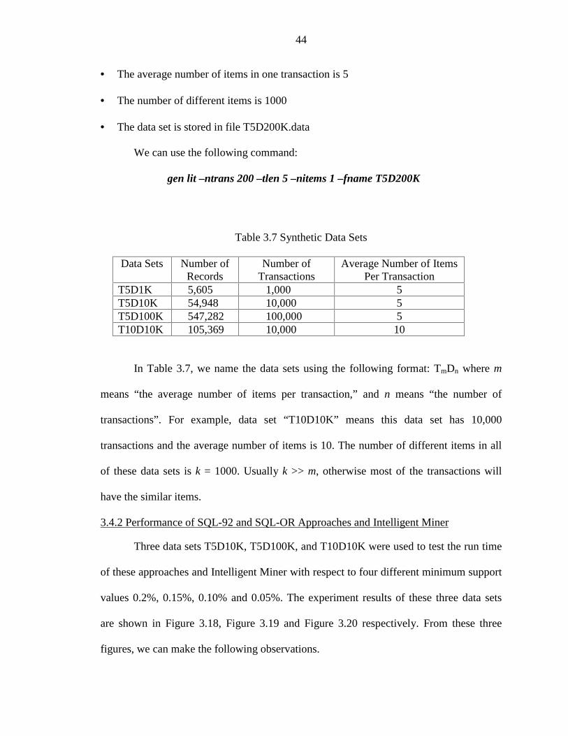
44
• The average number of items in one transaction is 5
• The number of different items is 1000
• The data set is stored in file T5D200K.data
We can use the following command:
gen lit –ntrans 200 –tlen 5 –nitems 1 –fname T5D200K
Table 3.7 Synthetic Data Sets
Data Sets Number ofRecords
Number ofTransactions
Average Number of ItemsPer Transaction
T5D1K 5,605 1,000 5T5D10K 54,948 10,000 5T5D100K 547,282 100,000 5T10D10K 105,369 10,000 10
In Table 3.7, we name the data sets using the following format: TmDn where m
means “the average number of items per transaction,” and n means “the number of
transactions”. For example, data set “T10D10K” means this data set has 10,000
transactions and the average number of items is 10. The number of different items in all
of these data sets is k = 1000. Usually k >> m, otherwise most of the transactions will
have the similar items.
3.4.2 Performance of SQL-92 and SQL-OR Approaches and Intelligent Miner
Three data sets T5D10K, T5D100K, and T10D10K were used to test the run time
of these approaches and Intelligent Miner with respect to four different minimum support
values 0.2%, 0.15%, 0.10% and 0.05%. The experiment results of these three data sets
are shown in Figure 3.18, Figure 3.19 and Figure 3.20 respectively. From these three
figures, we can make the following observations.
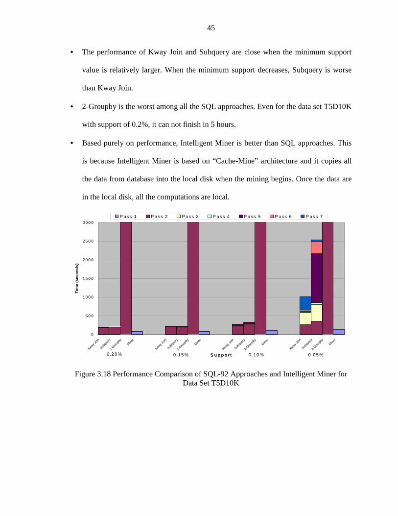
45
• The performance of Kway Join and Subquery are close when the minimum support
value is relatively larger. When the minimum support decreases, Subquery is worse
than Kway Join.
• 2-Groupby is the worst among all the SQL approaches. Even for the data set T5D10K
with support of 0.2%, it can not finish in 5 hours.
• Based purely on performance, Intelligent Miner is better than SQL approaches. This
is because Intelligent Miner is based on “Cache-Mine” architecture and it copies all
the data from database into the local disk when the mining begins. Once the data are
in the local disk, all the computations are local.
0
50 0
1 00 0
1 50 0
2 00 0
2 50 0
3 00 0
Kway Jo
in
Subqu
ery
2-Gro
upby
Mine
r
Kway Jo
in
Subqu
ery
2-Gro
upby
Mine
r
Kway Jo
in
Subqu
ery
2-Gro
upby
Mine
r
Kway Jo
in
Subqu
ery
2-Gro
upby
Mine
r
S u p p o rt
Tim
e (s
eco
nd
s)
P a ss 1 P a ss 2 P as s 3 P as s 4 P ass 5 P a ss 6 P a ss 7
0 .2 0% 0 .10 %0 .15% 0 .05 %
Figure 3.18 Performance Comparison of SQL-92 Approaches and Intelligent Miner forData Set T5D10K

46
0
5 0 0
1 0 0 0
1 5 0 0
2 0 0 0
2 5 0 0
3 0 0 0
Kway Jo
in
Subqu
ery
2-Gro
upby
Mine
r
Kway Jo
in
Subqu
ery
2-Gro
upby
Mine
r
Kway Jo
in
Subqu
ery
2-Gro
upby
Mine
r
Kway Jo
in
Subqu
ery
2-Gro
upby
Mine
r
S u p p o r t
Tim
e (s
eco
nd
s)
P a s s 1 P a s s 2 P a s s 3 P a s s 4 P a s s 5 P a s s 6 P a s s 7
0 .2 0 % 0 .1 0 % 0 .0 5 %0 .1 5 %
Figure 3.19 Performance Comparison of SQL-92 Approaches and Intelligent Miner forData Set T5D100K
0
5 00
10 00
15 00
20 00
25 00
30 00
Kway Jo
in
Subqu
ery
2-Gro
upby
Mine
r
Kway Jo
in
Subqu
ery
2-Gro
upby
Mine
r
Kway Jo
in
Subqu
ery
2-Gro
upby
Mine
r
S u p p o rt
Tim
e (s
eco
nd
s)
P a ss 1 P as s 2 P a ss 3 P as s 4 P a ss 5 P as s 6 P a ss 7
0 .20% 0 .15% 0 .10%
Figure 3.20 Performance Comparison of SQL-92 Approaches and Intelligent Miner forData Set T10D10K

47
3.4.3 Scale-Up Experiments
We used different synthetic generated data sets to study the scale-up behavior
SQL approaches with respect to increasing number of records. We varied the number of
records using the different number of transactions and the average number of items per
transaction. Figure 3.21 shows how these SQL approaches scales up as the number of
records is increased from 5K to 500K. The minimum support and confidence values are
constant for all the four data sets, which are 0.2% and 50% respectively.
From Figure 3.21 we observed that run time scale quite linearly as the number of
records increased. It also shows that both Kway Join and Subquery approaches have the
similar scale-up behavior. The 2-Groupby approach has not been included in Figure 3.21
because it can not complete even the smallest data sets T5D1K in 2-3 hours.
0
1 0 0
2 0 0
3 0 0
4 0 0
5 0 0
6 0 0
7 0 0
8 0 0
9 0 0
0 5 0 K 5 0 0 K
N u m b e r o f R e c o r d s
Tim
e (s
eco
nd
s)
K w a y J o in S u b q u e ry
Figure 3.21 Scale-Up Experiments for SQL-92 Approaches

48
CHAPTER 4VISUALIZATION OF ASSOCIATION RULES
Visualization is the process of transforming data, information, and knowledge into
visual form making use of human’s natural visual capabilities [GER1998]. There are
three kinds of visualization categories in data mining [GRI1995]. The first approach is to
use visualization techniques to present the information obtained from mining the data in
the database, and this approach is conventionally being used in many data mining tools.
The second approach is to visualize the data in database before applying the data mining
algorithms. By using this approach, the user can have a better understanding of the data.
The third approach is to use visualization techniques to complement the data mining
techniques. It is also known as visual data mining allowing user to understand the data
mining process and the data mining models being used. In this chapter, we will focus on
the first approach by reviewing the related work of visualization in data mining, then we
provide our design of rule table and 3-D rule visualization system for association rule.
4.1 Related Work
In this section, we first summarize the different categories of data visualization
techniques for data mining, then visualization techniques for association rule will be
reviewed.
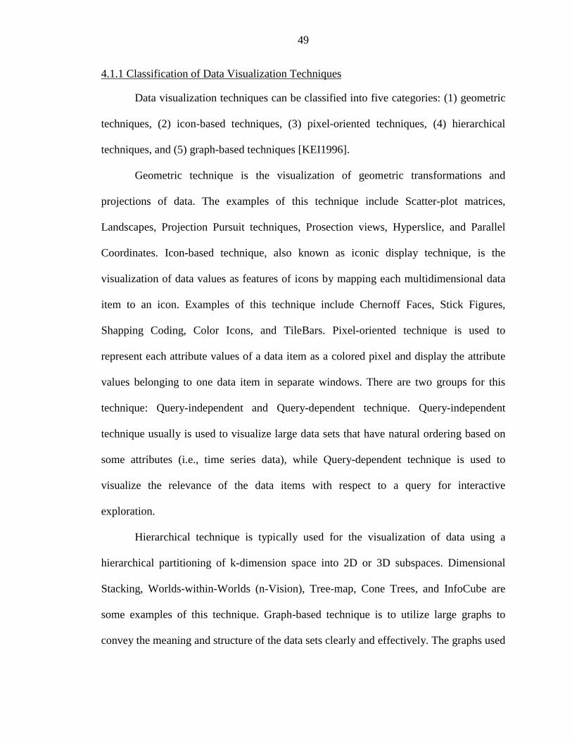
49
4.1.1 Classification of Data Visualization Techniques
Data visualization techniques can be classified into five categories: (1) geometric
techniques, (2) icon-based techniques, (3) pixel-oriented techniques, (4) hierarchical
techniques, and (5) graph-based techniques [KEI1996].
Geometric technique is the visualization of geometric transformations and
projections of data. The examples of this technique include Scatter-plot matrices,
Landscapes, Projection Pursuit techniques, Prosection views, Hyperslice, and Parallel
Coordinates. Icon-based technique, also known as iconic display technique, is the
visualization of data values as features of icons by mapping each multidimensional data
item to an icon. Examples of this technique include Chernoff Faces, Stick Figures,
Shapping Coding, Color Icons, and TileBars. Pixel-oriented technique is used to
represent each attribute values of a data item as a colored pixel and display the attribute
values belonging to one data item in separate windows. There are two groups for this
technique: Query-independent and Query-dependent technique. Query-independent
technique usually is used to visualize large data sets that have natural ordering based on
some attributes (i.e., time series data), while Query-dependent technique is used to
visualize the relevance of the data items with respect to a query for interactive
exploration.
Hierarchical technique is typically used for the visualization of data using a
hierarchical partitioning of k-dimension space into 2D or 3D subspaces. Dimensional
Stacking, Worlds-within-Worlds (n-Vision), Tree-map, Cone Trees, and InfoCube are
some examples of this technique. Graph-based technique is to utilize large graphs to
convey the meaning and structure of the data sets clearly and effectively. The graphs used
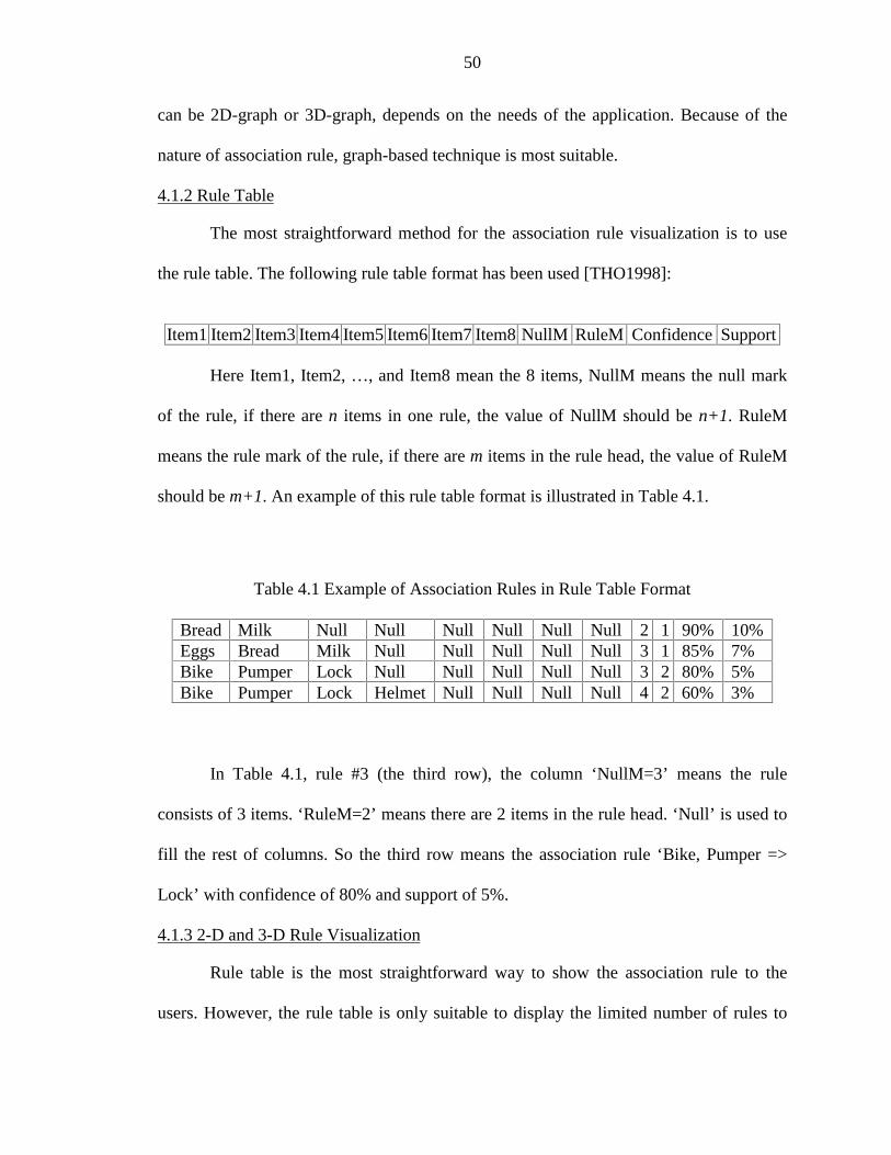
50
can be 2D-graph or 3D-graph, depends on the needs of the application. Because of the
nature of association rule, graph-based technique is most suitable.
4.1.2 Rule Table
The most straightforward method for the association rule visualization is to use
the rule table. The following rule table format has been used [THO1998]:
Item1 Item2 Item3 Item4 Item5 Item6 Item7 Item8 NullM RuleM Confidence Support
Here Item1, Item2, …, and Item8 mean the 8 items, NullM means the null mark
of the rule, if there are n items in one rule, the value of NullM should be n+1. RuleM
means the rule mark of the rule, if there are m items in the rule head, the value of RuleM
should be m+1. An example of this rule table format is illustrated in Table 4.1.
Table 4.1 Example of Association Rules in Rule Table Format
Bread Milk Null Null Null Null Null Null 2 1 90% 10%Eggs Bread Milk Null Null Null Null Null 3 1 85% 7%Bike Pumper Lock Null Null Null Null Null 3 2 80% 5%Bike Pumper Lock Helmet Null Null Null Null 4 2 60% 3%
In Table 4.1, rule #3 (the third row), the column ‘NullM=3’ means the rule
consists of 3 items. ‘RuleM=2’ means there are 2 items in the rule head. ‘Null’ is used to
fill the rest of columns. So the third row means the association rule ‘Bike, Pumper =>
Lock’ with confidence of 80% and support of 5%.
4.1.3 2-D and 3-D Rule Visualization
Rule table is the most straightforward way to show the association rule to the
users. However, the rule table is only suitable to display the limited number of rules to

51
the users. If the user needs to have a global view of all the rules, the rule table is not a
suitable approach.
Several commercial data mining products provide a visualization module. Becker
[BEC1998] presented a technique to visualize the decision table classifiers. In this
visualization module, the interactive drill down, drill-up, drill-through, filtering, and
animation gave the user more flexibility.
As to association rule visualization, lots of work has been done using directed
graph, 2-D matrix, and 3-D visualization.
4.1.3.1 Directed Graph
Directed Graph is used as the association rule visualization technique in the
IBM’s data mining software “Intelligent Miner”. In directed graph, the nodes of a
directed graph represent the items, and the edges represent the associations. Figure 4.1
shows 3 association rules (Bread => Milk; Bread => Butter; Eggs => Bread + Milk).
Milk
Bread
Bread Eggs
Butter Milk
Figure 4.1 Association Rules Represented by Directed Graph
The confidence and support of the rules can be depicted using different colors and
width of arrow. For example, the wider the length of arrow, the more confidence the rule
has.
Directed Graph is a good visualization technique when the number of rules and
the items in each rule is very small. When the number of rules and the items in each rule
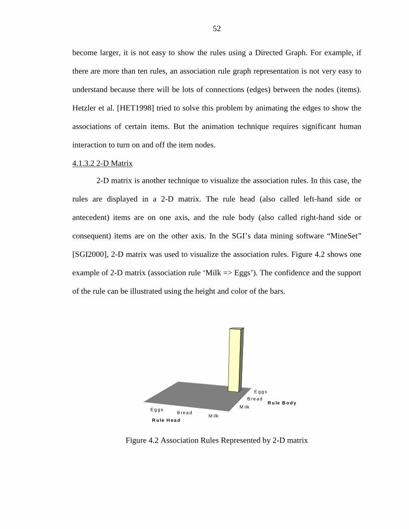
52
become larger, it is not easy to show the rules using a Directed Graph. For example, if
there are more than ten rules, an association rule graph representation is not very easy to
understand because there will be lots of connections (edges) between the nodes (items).
Hetzler et al. [HET1998] tried to solve this problem by animating the edges to show the
associations of certain items. But the animation technique requires significant human
interaction to turn on and off the item nodes.
4.1.3.2 2-D Matrix
2-D matrix is another technique to visualize the association rules. In this case, the
rules are displayed in a 2-D matrix. The rule head (also called left-hand side or
antecedent) items are on one axis, and the rule body (also called right-hand side or
consequent) items are on the other axis. In the SGI’s data mining software “MineSet”
[SGI2000], 2-D matrix was used to visualize the association rules. Figure 4.2 shows one
example of 2-D matrix (association rule ‘Milk => Eggs’). The confidence and the support
of the rule can be illustrated using the height and color of the bars.
E g g sB re a d
M ilk
M ilk
B re a d
E g g s
R u le H e a d
R u le B o d y
Figure 4.2 Association Rules Represented by 2-D matrix

53
But Figure 4.2 only can show the ‘one-to-one’ relationship, that is, only one item
can be allowed in rule head and rule body, respectively. For example, in Figure 4.3, it is
almost impossible to tell whether there is only one rule (Bread + Milk => Eggs) or there
are two separate rules (Bread => Eggs; Milk => Eggs).
E g g sB re a d
M ilk
M ilk
B re a d
E g g s
R u le H e ad
R u le B o d y
Figure 4.3 Association Rules Represented by 2-D Matrix
MineSet tried to allow multiple items in rule head and rule body by grouping the
each of the items combinations in rule head or rule body as one unit. Figure 4.4 shows
that rule “Bread + Milk => Eggs” can be plotted by adding one more unit “Bread + Milk”
in one axis. The other rule in Figure 4.4 is “Milk => Eggs”.
Although Figure 4.4 can show ‘many-to-many’ relationship, it works well only
when the items in the rule head and rule body is very few. When the number of items in
the rule head is large, the number of units is expected to be very large if there are lots of
combinations. This is because all combinations of items in the rule head and the rule
body will be added in X or Y axes as one unit.
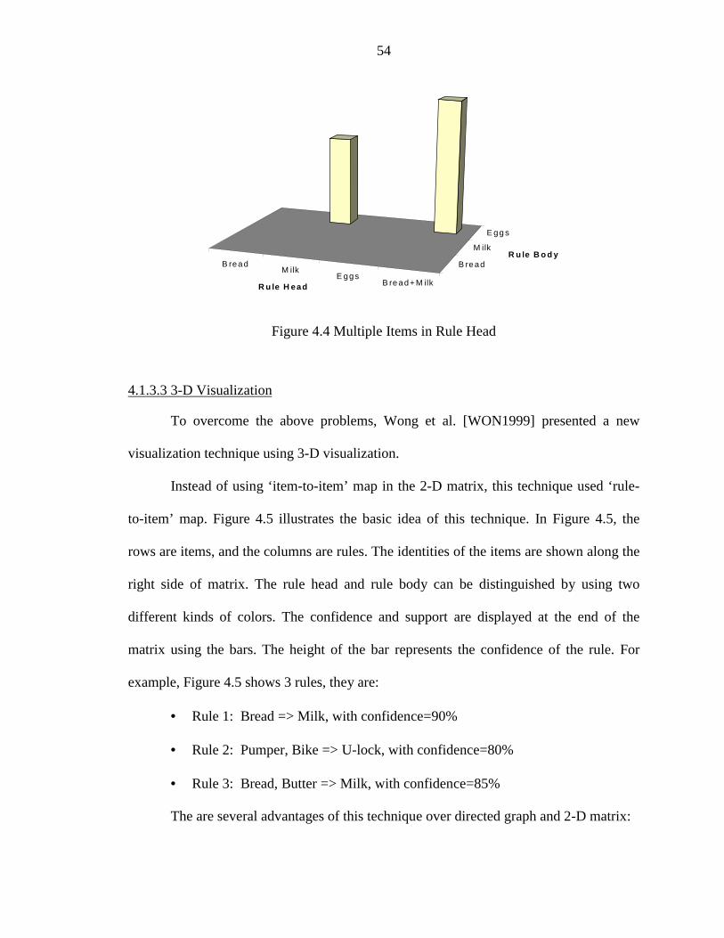
54
B readM ilk
E ggsB re ad+ M ilk
B read
M ilk
E gg s
R u le H ead
R u le B o d y
Figure 4.4 Multiple Items in Rule Head
4.1.3.3 3-D Visualization
To overcome the above problems, Wong et al. [WON1999] presented a new
visualization technique using 3-D visualization.
Instead of using ‘item-to-item’ map in the 2-D matrix, this technique used ‘rule-
to-item’ map. Figure 4.5 illustrates the basic idea of this technique. In Figure 4.5, the
rows are items, and the columns are rules. The identities of the items are shown along the
right side of matrix. The rule head and rule body can be distinguished by using two
different kinds of colors. The confidence and support are displayed at the end of the
matrix using the bars. The height of the bar represents the confidence of the rule. For
example, Figure 4.5 shows 3 rules, they are:
• Rule 1: Bread => Milk, with confidence=90%
• Rule 2: Pumper, Bike => U-lock, with confidence=80%
• Rule 3: Bread, Butter => Milk, with confidence=85%
The are several advantages of this technique over directed graph and 2-D matrix:

55
1. The identity of individual items within the rule head is clearly shown.
2. The metadata such as confidence and support are shown at the end of the matrix, so
the whole view is clearer to the users.
3. In theory, there is no upper limit on the number of items in the rule head.
4. It is not needed any more to create the additional units in the matrix because of the
combination of the items in the rule head. The number of unites in axes is depend
only on the number of items and the number of rules.
Because 3-D visualization has the above advantages, it is a big improvement over
the directed graph and 2-D matrix visualization.
4.2 Rule Table
In Table 4.1, the user has to distinguish the rule head and rule body by the value
of ‘NULLM’ and ‘RULEM’. It’s very difficult for the user to understand the rules. To
address this problem, we can introduce the following rule table format.
Rule Head ‘Imply’ Symbol Rule Body Confidence Support
So all the rules in Table 4.1 can be represented by this format in Table 4.2.
Table 4.2 Example of Association Rules in Rule Table Format
Bread => Milk 90% 10%Eggs => Bread, Milk 85% 7%Bike, Pumper => Lock 80% 5%Bike, Pumper => Lock, Helmet 60% 3%
There are several reasons for the new rule table format:
1. In Table 4.1, the maximum item numbers in the association rules is fixed. For
example, the maximum item number in Table 4.1 is 8. It can not show the rules that

56
have more than 8 items. If we need to display more than 8 items, the additional
columns need to be added. However, the new rule table format does not have this
problem.
1 2 3
Pumper
Bike
Bread
ButterCarHelmetInsuranceMilkRegisterU-lock
0
10
20
30
40
50
60
70
80
90
Confidence (%)
Rule
Item
Figure 4.5 3-D Visualization of Association Rules
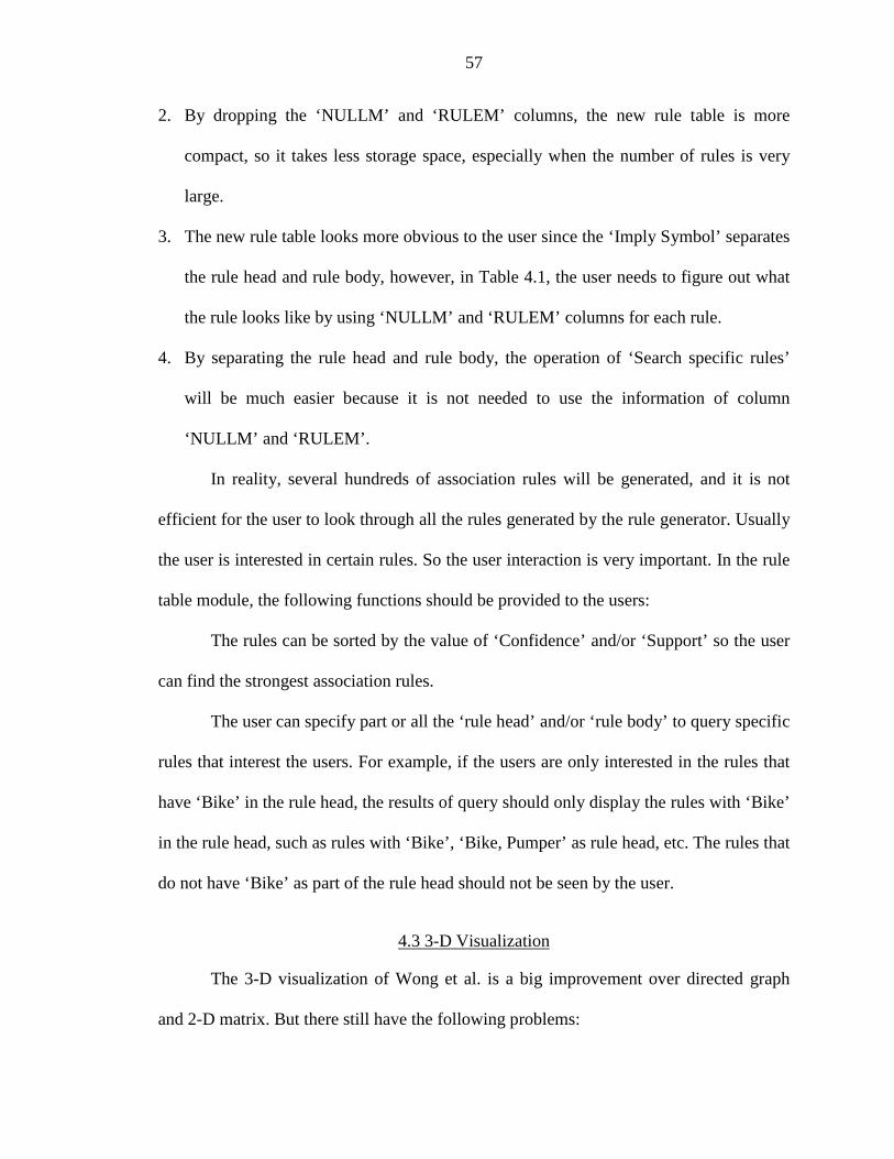
57
2. By dropping the ‘NULLM’ and ‘RULEM’ columns, the new rule table is more
compact, so it takes less storage space, especially when the number of rules is very
large.
3. The new rule table looks more obvious to the user since the ‘Imply Symbol’ separates
the rule head and rule body, however, in Table 4.1, the user needs to figure out what
the rule looks like by using ‘NULLM’ and ‘RULEM’ columns for each rule.
4. By separating the rule head and rule body, the operation of ‘Search specific rules’
will be much easier because it is not needed to use the information of column
‘NULLM’ and ‘RULEM’.
In reality, several hundreds of association rules will be generated, and it is not
efficient for the user to look through all the rules generated by the rule generator. Usually
the user is interested in certain rules. So the user interaction is very important. In the rule
table module, the following functions should be provided to the users:
The rules can be sorted by the value of ‘Confidence’ and/or ‘Support’ so the user
can find the strongest association rules.
The user can specify part or all the ‘rule head’ and/or ‘rule body’ to query specific
rules that interest the users. For example, if the users are only interested in the rules that
have ‘Bike’ in the rule head, the results of query should only display the rules with ‘Bike’
in the rule head, such as rules with ‘Bike’, ‘Bike, Pumper’ as rule head, etc. The rules that
do not have ‘Bike’ as part of the rule head should not be seen by the user.
4.3 3-D Visualization
The 3-D visualization of Wong et al. is a big improvement over directed graph
and 2-D matrix. But there still have the following problems:

58
1. It is best for the ‘many-to-one’ relationship. That is, the rule body has only one item.
When the rule body has more than 1 item, the matrix floor is covered with many
blocks.
2. The users have to distinguish the rule head and rule body by the different color of
blocks. Usually not all the items in the rule head will be displayed together, so the
users can not figure out what is the rule looks like at the first glance, especially when
the number of items in the rule body is more than 1. Figure 4.7 shows this problem. In
Figure 4.7, Rule 4 means rule ‘b, e, i, j => d, g’ with confidence=58%. But because
not all the items in the rule head display at the one end, and not all the items in the
rule body display at the other end, it is not clear to the user of how the rule looks like.
It is idea if all the items in the rule head can be put on the one end, and all the items in
the rule body can by put on the other end so the user can see the rules very clearly.
3. Although it can show lots of rules at the same time, the interaction between the
visualization system and the user is definitely needed because most of the time, the
users are only interested in some specific rules with some specific items in the rule
head and/or rule body. So the system should provide the user a very good interface to
interact with the system.
To address the above three problems, the new 3-D visualization system should try
to achieve the following goals:
1. It should have a very good interactive graphic user interface. The user can sort, filter
the rules according to the user’s interest.
2. The items in the rule head and the items in the rule body should be separated very
obviously. That means, it is the best if all the items in the rule head are at the one end,
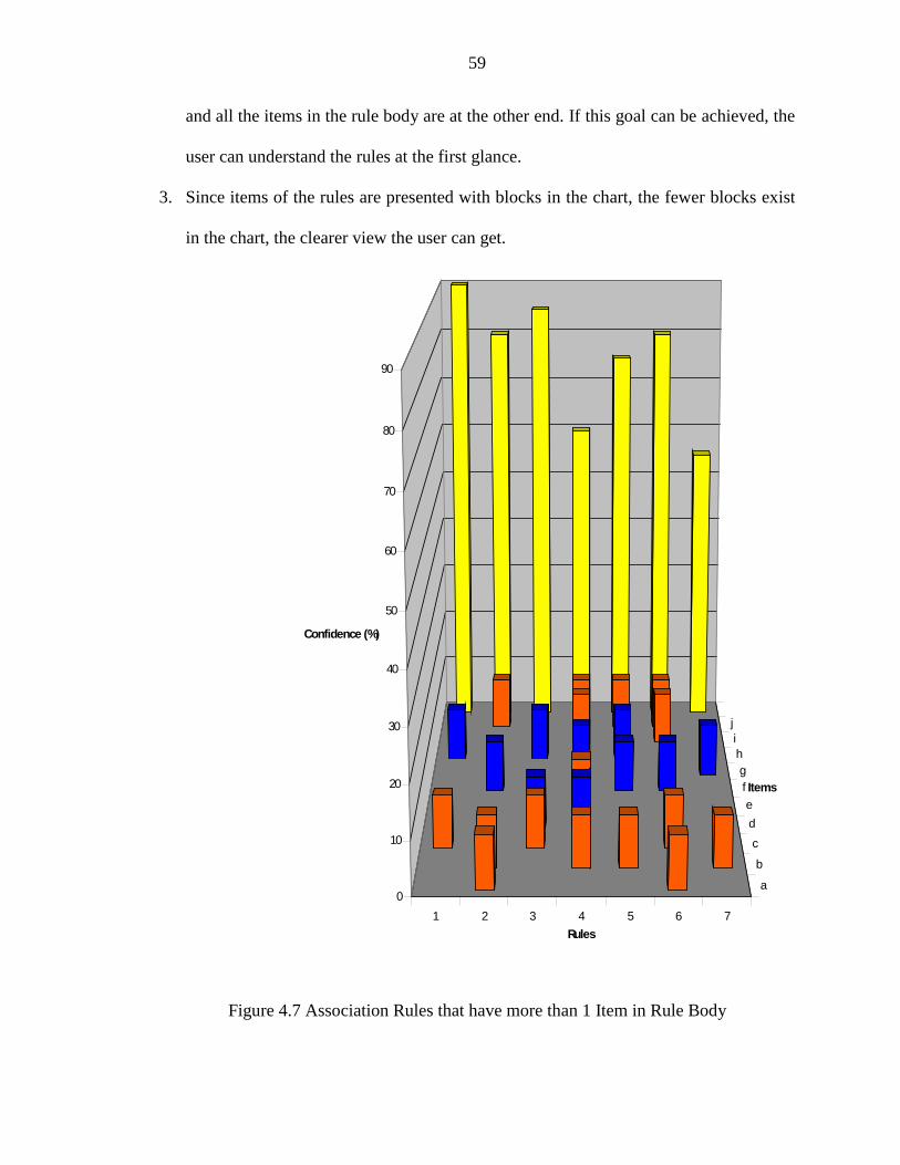
59
and all the items in the rule body are at the other end. If this goal can be achieved, the
user can understand the rules at the first glance.
3. Since items of the rules are presented with blocks in the chart, the fewer blocks exist
in the chart, the clearer view the user can get.
1 2 3 4 5 6 7
a
b
c
d
e
fg
hij
0
10
20
30
40
50
60
70
80
90
Confidence (%)
Rules
Items
Figure 4.7 Association Rules that have more than 1 Item in Rule Body

60
Based on the above goals, we improved the 3-D visualization technique of Wong
et al. by adding the following new features:
1. There will be a graphic user interface provided to the user to do the sorting, filtering,
animation, etc. It will be very flexible for the user to use. Goal #1 is achieved. Details
of the user interface will be discussed in Chapter 6.
2. The items in the rule body are shown in axis X using the text. So the rule head and
rule body is visually separated and the user can see what the rules look like at the first
glance. Goal #2 is achieved.
3. Removes the blocks of items in rule body, as a result, on the chart only the items in
the rule head remains, and only one color is enough, and there are fewer blocks on the
chart. Goal #3 is achieved.
Figure 4.8 illustrates the basic idea of the above modification.

61
1 2 3 4 5 6 7
a
b
c
d
e
f
g
h
i
j
k
l
Rules
Head
Support
Confidence
h f d, h d, gf, h f g
0
50%
100%
1.0
2.0
3.0
Figure 4.8 Association Rule Visualization

62
CHAPTER 5SYSTEM IMPLEMENTATION
In the previous chapters, we presented the several different association rule
algorithms, and then provided our design of association rule visualization technique. The
input of the rule generation algorithm is a table with two columns “tid, item”, and the
output is a table with each rule occupies one row. However, in reality, the data are
usually not exactly in the form of “tid, item”, and some of them are in text format, instead
of integer format. For example, in the supermarket, each transaction consists of
transaction id, and items that each customer buys. In this case, the date and time may
work as the transaction id, and the items can be identified by their names. To fit this kind
of data set into the input format of our rule generation algorithm, we should have a very
good graphic user interface (GUI) for the user to manipulate their existing data set to feed
to our rule generation algorithm. We choose Java as the programming language for this
project based on the following reasons:
1. Java program is platform independent. Instead of generating the executable
machine instructions by the C++ compiler, Java compiler outputs Java byte
codes. Java byte codes are instructions written for some virtual Java machines
that do not really exist. These byte codes run through the Java Virtual
Machine (JVM), which works as an interpreter to execute the Java byte codes.
There is a different JVM emulator for each different type of machines, so Java
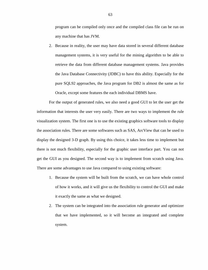
63
program can be compiled only once and the compiled class file can be run on
any machine that has JVM.
2. Because in reality, the user may have data stored in several different database
management systems, it is very useful for the mining algorithm to be able to
retrieve the data from different database management systems. Java provides
the Java Database Connectivity (JDBC) to have this ability. Especially for the
pure SQL92 approaches, the Java program for DB2 is almost the same as for
Oracle, except some features the each individual DBMS have.
For the output of generated rules, we also need a good GUI to let the user get the
information that interests the user very easily. There are two ways to implement the rule
visualization system. The first one is to use the existing graphics software tools to display
the association rules. There are some softwares such as SAS, ArcView that can be used to
display the designed 3-D graph. By using this choice, it takes less time to implement but
there is not much flexibility, especially for the graphic user interface part. You can not
get the GUI as you designed. The second way is to implement from scratch using Java.
There are some advantages to use Java compared to using existing software:
1. Because the system will be built from the scratch, we can have whole control
of how it works, and it will give us the flexibility to control the GUI and make
it exactly the same as what we designed.
2. The system can be integrated into the association rule generator and optimizer
that we have implemented, so it will become an integrated and complete
system.

64
3. By using Java, it will not only run as the application, also it can be put on the
web and run as the applet.
4. Java provides a set of Java 3D APIs that serve as the interface to a
sophisticated three-dimensional graphics rendering system. A Java 3D
program creates instances of Java 3D objects and places them into a scene
graph data structure. Despite all of the 3D functionality, the Java 3D API is
still straightforward to use.
Because of the above reasons, we choose Java 3D to implement the association
rule visualization module.
In this chapter, the system architecture of our software is presented in Section 5.1.
The interfaces of rule generator and rule visualization, as well as their implementations
are detailed in Section 5.2 and 5.3.
5.1 System Architecture
Our system is based on the two-tier model because no business logic is
incorporated in our system. The system architecture is shown in Figure 5.1.
In Figure 5.1, the database resides in the server machine. The stored procedures
(Oracle) and UDFs (DB2) also reside in the server side. Our Java application runs in the
client machine. It consists of several modules: LogIn, Rule Generator, and Visualization
module. LogIn module is used to connect to the database server. Rule Generator is used
to mining the association rules given the information provided by the user. Visualization
module consists of two sub-modules Rule table and 3-D visualization. These modules can
be accessed using the Main window. The interfaces and their implementation are
presented in the following sections.
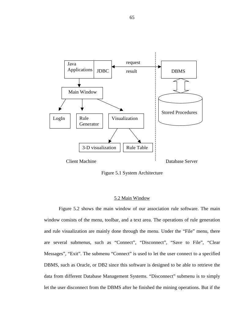
65
Figure 5.1 System Architecture
5.2 Main Window
Figure 5.2 shows the main window of our association rule software. The main
window consists of the menu, toolbar, and a text area. The operations of rule generation
and rule visualization are mainly done through the menu. Under the “File” menu, there
are several submenus, such as “Connect”, “Disconnect”, “Save to File”, “Clear
Messages”, “Exit”. The submenu “Connect” is used to let the user connect to a specified
DBMS, such as Oracle, or DB2 since this software is designed to be able to retrieve the
data from different Database Management Systems. “Disconnect” submenu is to simply
let the user disconnect from the DBMS after he finished the mining operations. But if the
JavaApplications JDBC
request
DBMS
Client Machine Database Server
result
LogIn RuleGenerator
Visualization
Rule Table3-D visualization
Stored Procedures
Main Window
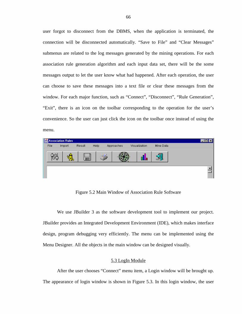
66
user forgot to disconnect from the DBMS, when the application is terminated, the
connection will be disconnected automatically. “Save to File” and “Clear Messages”
submenus are related to the log messages generated by the mining operations. For each
association rule generation algorithm and each input data set, there will be the some
messages output to let the user know what had happened. After each operation, the user
can choose to save these messages into a text file or clear these messages from the
window. For each major function, such as “Connect”, “Disconnect”, “Rule Generation”,
“Exit”, there is an icon on the toolbar corresponding to the operation for the user’s
convenience. So the user can just click the icon on the toolbar once instead of using the
menu.
Figure 5.2 Main Window of Association Rule Software
We use JBuilder 3 as the software development tool to implement our project.
JBuilder provides an Integrated Development Environment (IDE), which makes interface
design, program debugging very efficiently. The menu can be implemented using the
Menu Designer. All the objects in the main window can be designed visually.
5.3 LogIn Module
After the user chooses “Connect” menu item, a Login window will be brought up.
The appearance of login window is shown in Figure 5.3. In this login window, the user
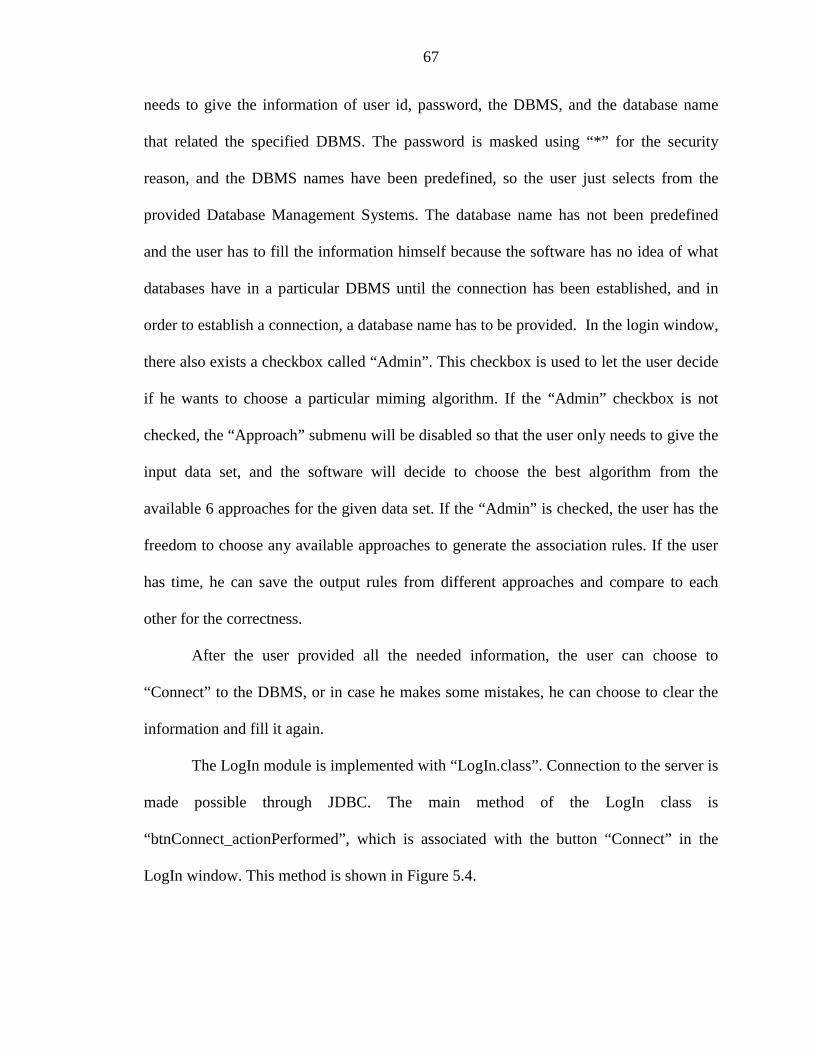
67
needs to give the information of user id, password, the DBMS, and the database name
that related the specified DBMS. The password is masked using “*” for the security
reason, and the DBMS names have been predefined, so the user just selects from the
provided Database Management Systems. The database name has not been predefined
and the user has to fill the information himself because the software has no idea of what
databases have in a particular DBMS until the connection has been established, and in
order to establish a connection, a database name has to be provided. In the login window,
there also exists a checkbox called “Admin”. This checkbox is used to let the user decide
if he wants to choose a particular miming algorithm. If the “Admin” checkbox is not
checked, the “Approach” submenu will be disabled so that the user only needs to give the
input data set, and the software will decide to choose the best algorithm from the
available 6 approaches for the given data set. If the “Admin” is checked, the user has the
freedom to choose any available approaches to generate the association rules. If the user
has time, he can save the output rules from different approaches and compare to each
other for the correctness.
After the user provided all the needed information, the user can choose to
“Connect” to the DBMS, or in case he makes some mistakes, he can choose to clear the
information and fill it again.
The LogIn module is implemented with “LogIn.class”. Connection to the server is
made possible through JDBC. The main method of the LogIn class is
“btnConnect_actionPerformed”, which is associated with the button “Connect” in the
LogIn window. This method is shown in Figure 5.4.
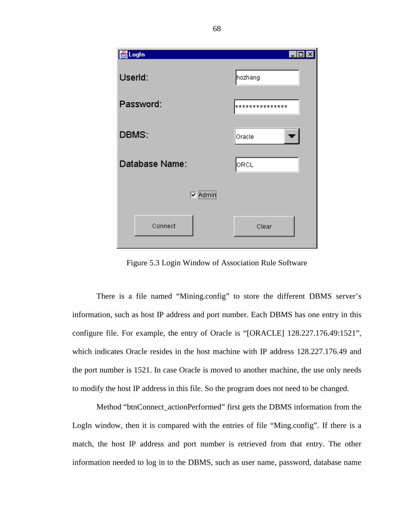
68
Figure 5.3 Login Window of Association Rule Software
There is a file named “Mining.config” to store the different DBMS server’s
information, such as host IP address and port number. Each DBMS has one entry in this
configure file. For example, the entry of Oracle is “[ORACLE] 128.227.176.49:1521”,
which indicates Oracle resides in the host machine with IP address 128.227.176.49 and
the port number is 1521. In case Oracle is moved to another machine, the use only needs
to modify the host IP address in this file. So the program does not need to be changed.
Method “btnConnect_actionPerformed” first gets the DBMS information from the
LogIn window, then it is compared with the entries of file “Ming.config”. If there is a
match, the host IP address and port number is retrieved from that entry. The other
information needed to log in to the DBMS, such as user name, password, database name
69
can be obtained through the user’s input in the LogIn window. Once all the information is
ready, JDBC first loads the corresponding database driver using the method
“Class.forName”. After the driver is loaded, a connection can be made using the method
“DriverManager.getConnection (url, user, passwd)”. The highlighted lines of code in
Figure 5.4 illustrates how to load the database driver and how to make a connection to the
server.
Figure 5.4 btnConnect_actionPerformed Method
void btnConnect_actionPerformed(ActionEvent e) { fin = new FileInputStream("Mining.config"); while((bytes_read = fin.read(buffer)) != -1); fileText = new String(buffer); Vector vc=new Vector(); StringTokenizer st = new StringTokenizer(fileText); while (st.hasMoreTokens())
vc.addElement(st.nextToken()); for(int i=0;i<vc.size();i++) { if(vc.elementAt(i).toString().equals("[ORACLE]")) server = vc.elementAt(i+1).toString(); } if ( (cmbDBMS.getSelectedItem().toString()).equals("DB2") ) { Class.forName("COM.ibm.db2.jdbc.app.DB2Driver"); //for .app url = "jdbc:db2:"; url = url.concat(db); } else if ( (cmbDBMS.getSelectedItem().toString()).equals("Oracle") ) { Class.forName("oracle.jdbc.driver.OracleDriver");// url = "jdbc:oracle:thin:@tokyo.dbcenter.cise.ufl.edu:1521"// server = "128.227.176.49"; url = "jdbc:oracle:thin:@" + server + ":"; url = url.concat(db); } con = DriverManager.getConnection (url, user, passwd);} // end of btnConnect_actionPerformed

70
5.4 Rule Generator
For each input data set, some parameters have to be specified by the user for the
association rule generation. This kind of information can be input by the Parameter Input
window. Parameter Input window is shown in Figure 5.5. For the data source, because
the data is not always in the same table, and sometimes it is needed to obtain the data
from two or more different tables, the user should have the ability to select multiple
tables as the data source. For this reason, the available table names have been populated
in the list box. The user can choose multiple tables by using “Shift” or “Control” key. For
the multiple tables, the “Join” and “Union” operations are also provided to let the user
manipulate the data source from multiple tables and combine them into one table. The
user may also want to specify the lowest support and confidence value to get the
interested association rules. The value of stop level is used to let the user decide that after
how much passes that the user wants the rule generation needs to be canceled. The
“Statistics” button is used to show the user some basic statistics (such as number of
transactions, number of rows, number of different items, average number of items in each
transaction, etc) of the selected tables. After all of the information is completed, the user
can click the “Generate Rules” to begin to merge the data from different tables. Then the
association rule generation algorithm will be called to generate the rules.
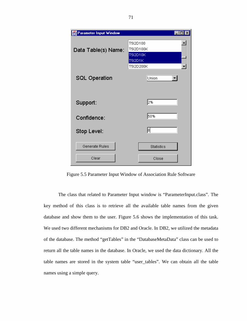
71
Figure 5.5 Parameter Input Window of Association Rule Software
The class that related to Parameter Input window is “ParameterInput.class”. The
key method of this class is to retrieve all the available table names from the given
database and show them to the user. Figure 5.6 shows the implementation of this task.
We used two different mechanisms for DB2 and Oracle. In DB2, we utilized the metadata
of the database. The method “getTables” in the “DatabaseMetaData” class can be used to
return all the table names in the database. In Oracle, we used the data dictionary. All the
table names are stored in the system table “user_tables”. We can obtain all the table
names using a simple query.

72
Figure 5.6 Retrieve All the Table Names Available in the Database
5.5 Visualization Module
In the association rule software, we implemented two kinds of rule visualization
tools to view the mining results: rule table and 3-D graphic. Each tool allows the user to
work in the interactive environment. This section describes these tools in detail.
5.5.1 Rule Table
Figure 5.7 shows the rule table visualization window. In this window, all the rules
shows according to the rule format introduced in Chapter 4. Because usually hundreds of
Statement stmt = LogIn.con.createStatement( );DatabaseMetaData dbmd = LogIn.con.getMetaData(); if(LogIn.cmbDBMS.getSelectedItem().toString().equals("DB2")){
String[] type={"TABLE"};ResultSet rs =dbmd.getTables("",LogIn.user_id.toUpperCase(),"",type);ResultSetMetaData rsmd = rs.getMetaData();
boolean more = rs.next(); while ( more ) { String rsts=rs.getString(3); tables.addElement(rsts); more = rs.next(); // move to next row } rs.close();} // end of first ’if’else if(LogIn.cmbDBMS.getSelectedItem().toString().equals("Oracle")){ String qs="select table_name from user_tables"; ResultSet rs=stmt.executeQuery( qs ); boolean more = rs.next(); while ( more ) { String rsts=rs.getString(1); tables.addElement(rsts); more = rs.next(); // move to next row } rs.close();} // end of ’if’stmt.close();
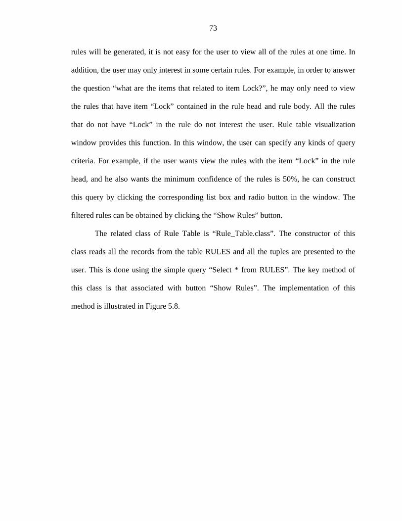
73
rules will be generated, it is not easy for the user to view all of the rules at one time. In
addition, the user may only interest in some certain rules. For example, in order to answer
the question “what are the items that related to item Lock?”, he may only need to view
the rules that have item “Lock” contained in the rule head and rule body. All the rules
that do not have “Lock” in the rule do not interest the user. Rule table visualization
window provides this function. In this window, the user can specify any kinds of query
criteria. For example, if the user wants view the rules with the item “Lock” in the rule
head, and he also wants the minimum confidence of the rules is 50%, he can construct
this query by clicking the corresponding list box and radio button in the window. The
filtered rules can be obtained by clicking the “Show Rules” button.
The related class of Rule Table is “Rule_Table.class”. The constructor of this
class reads all the records from the table RULES and all the tuples are presented to the
user. This is done using the simple query “Select * from RULES”. The key method of
this class is that associated with button “Show Rules”. The implementation of this
method is illustrated in Figure 5.8.
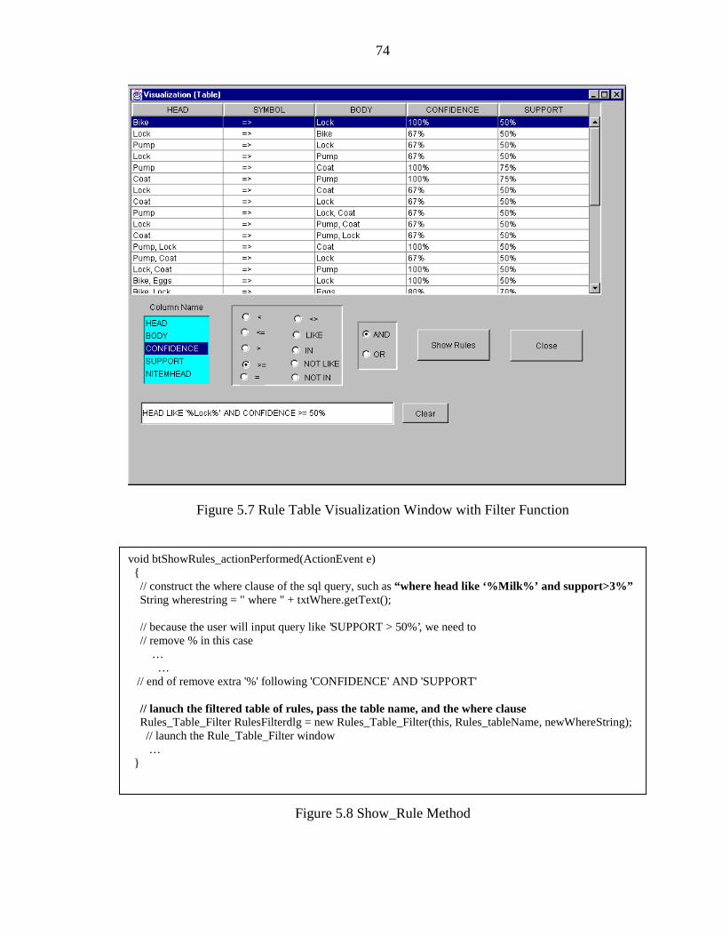
74
Figure 5.7 Rule Table Visualization Window with Filter Function
Figure 5.8 Show_Rule Method
void btShowRules_actionPerformed(ActionEvent e) { // construct the where clause of the sql query, such as “where head like ‘%Milk%’ and support>3%” String wherestring = " where " + txtWhere.getText();
// because the user will input query like ’SUPPORT > 50%’, we need to // remove % in this case … … // end of remove extra '%' following 'CONFIDENCE' AND 'SUPPORT'
// lanuch the filtered table of rules, pass the table name, and the where clause Rules_Table_Filter RulesFilterdlg = new Rules_Table_Filter(this, Rules_tableName, newWhereString); // launch the Rule_Table_Filter window … }

75
In Figure 5.8, the key point is to construct the where clause for the query. We
provide the user a set of standard SQL operators, such as ‘LIKE’, ‘NOT LIKE’, ‘IN’,
‘NOT IN’, ‘>’, ‘>=’, ‘AND’, ‘OR’, etc. For example, the query “Head Like ‘%Lock%’”
means that any rules that have “Lock” in the rule head satisfies the requirement. After the
user finished clicking the operators, the where clause is shown in a text box. The string in
the text box needs to be further processed (remove % from the support value, etc) for the
string becomes a where clause that any DBMS will accept it. At last, the final where
clause, together with the “RULE” table name, is passed to another class
Rule_Filter_Table to show the user filtered rules.
Figure 5.9 Rule Table Visualization Window with Sort Function

76
After filtering the rules, the user can also sort these rules by “confidence”, and
“support” columns with descending or ascending order. Figure 5.9 shows one example of
filtered rules with the query “HEAD LIKE ‘%Lock%’ AND CONFIDENCE >= 50%”
with the order of “confidence ascending, support descending”. This window also shows
the number of rules that satisfy the above query.
One issue about rule table is the feature of DBMS independence. The rule table
works on a table representation. Because all the operators provided to the user are
standard SQL operators, the corresponding SQL query can be executed in any DBMS. So
by using JDBC, the code for retrieving the rules from any DBMS is exactly the same and
no other extra codes are necessary for the different DBMSs.
5.5.2 3-D Visualization
Besides the rule table visualization tool, the other visualization tool is 3-D
graphic. First the rules are classified according to the number of items in the rule head.
Figure 5.10 shows the different categories of rules based on the number of the items in
the rule head. In Figure 5.10, it shows that there are three categories of rules, which have
1, 2, and 3 items in the rule head. In each category, the number of rules that falls into
each confidence or support interval (50%-60%, etc) is labeled. The labels for confidence
and support are in different colors. In Figure 5.10, it shows that for all the rules which
have 1 item in the rule head, 8 rules have the confidence between 60% to 70%, and 2
rules have the confidence between 90%-100%. As to the support, 9 rules have the value
of 40% to 50%, and only 1 rule has the value of 70%-80%. Double click the column bar
will invoke the 3-D visualization window that shows the rules with the particular number
of items in the rule head.
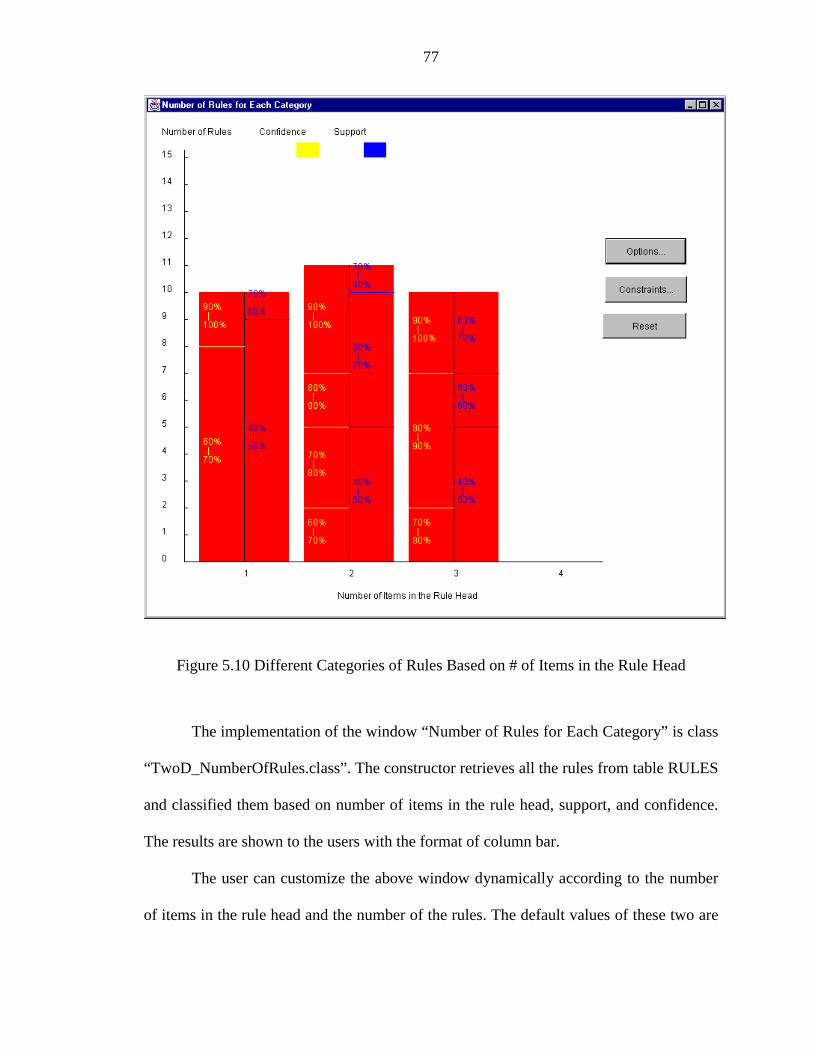
77
Figure 5.10 Different Categories of Rules Based on # of Items in the Rule Head
The implementation of the window “Number of Rules for Each Category” is class
“TwoD_NumberOfRules.class”. The constructor retrieves all the rules from table RULES
and classified them based on number of items in the rule head, support, and confidence.
The results are shown to the users with the format of column bar.
The user can customize the above window dynamically according to the number
of items in the rule head and the number of the rules. The default values of these two are
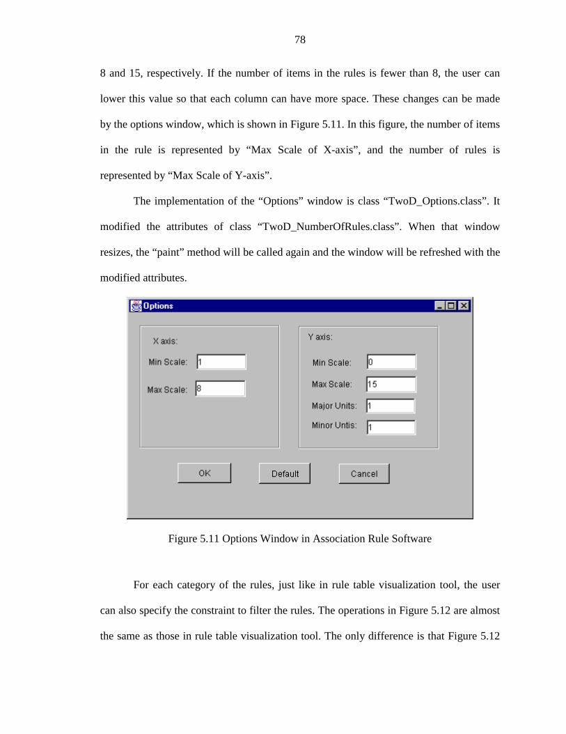
78
8 and 15, respectively. If the number of items in the rules is fewer than 8, the user can
lower this value so that each column can have more space. These changes can be made
by the options window, which is shown in Figure 5.11. In this figure, the number of items
in the rule is represented by “Max Scale of X-axis”, and the number of rules is
represented by “Max Scale of Y-axis”.
The implementation of the “Options” window is class “TwoD_Options.class”. It
modified the attributes of class “TwoD_NumberOfRules.class”. When that window
resizes, the “paint” method will be called again and the window will be refreshed with the
modified attributes.
Figure 5.11 Options Window in Association Rule Software
For each category of the rules, just like in rule table visualization tool, the user
can also specify the constraint to filter the rules. The operations in Figure 5.12 are almost
the same as those in rule table visualization tool. The only difference is that Figure 5.12
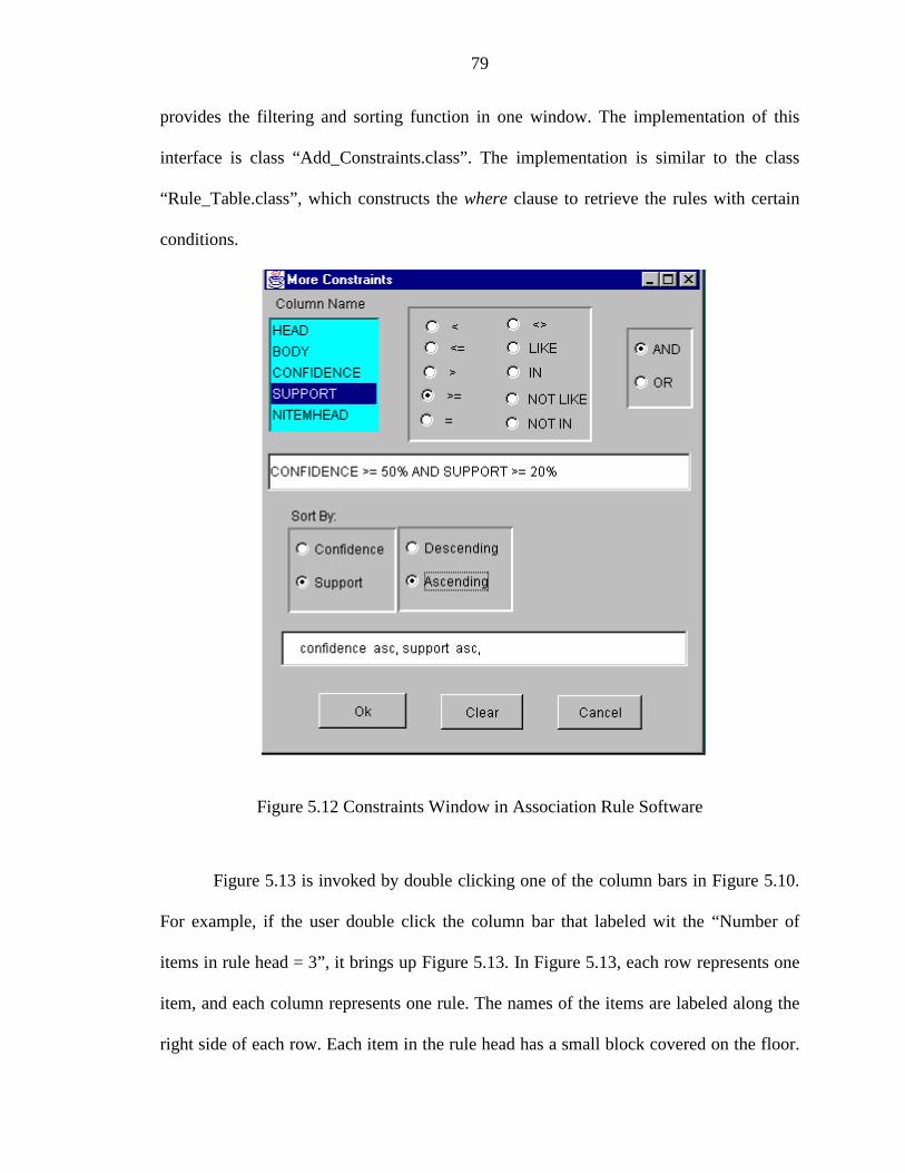
79
provides the filtering and sorting function in one window. The implementation of this
interface is class “Add_Constraints.class”. The implementation is similar to the class
“Rule_Table.class”, which constructs the where clause to retrieve the rules with certain
conditions.
Figure 5.12 Constraints Window in Association Rule Software
Figure 5.13 is invoked by double clicking one of the column bars in Figure 5.10.
For example, if the user double click the column bar that labeled wit the “Number of
items in rule head = 3”, it brings up Figure 5.13. In Figure 5.13, each row represents one
item, and each column represents one rule. The names of the items are labeled along the
right side of each row. Each item in the rule head has a small block covered on the floor.
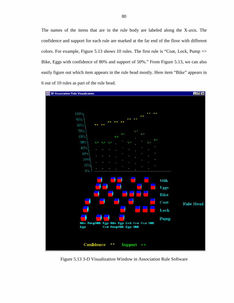
80
The names of the items that are in the rule body are labeled along the X-axis. The
confidence and support for each rule are marked at the far end of the floor with different
colors. For example, Figure 5.13 shows 10 rules. The first rule is “Coat, Lock, Pump =>
Bike, Eggs with confidence of 80% and support of 50%.” From Figure 5.13, we can also
easily figure out which item appears in the rule head mostly. Here item “Bike” appears in
6 out of 10 rules as part of the rule head.
Figure 5.13 3-D Visualization Window in Association Rule Software
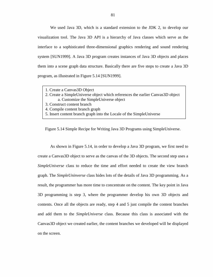
81
We used Java 3D, which is a standard extension to the JDK 2, to develop our
visualization tool. The Java 3D API is a hierarchy of Java classes which serve as the
interface to a sophisticated three-dimensional graphics rendering and sound rendering
system [SUN1999]. A Java 3D program creates instances of Java 3D objects and places
them into a scene graph data structure. Basically there are five steps to create a Java 3D
program, as illustrated in Figure 5.14 [SUN1999].
Figure 5.14 Simple Recipe for Writing Java 3D Programs using SimpleUniverse.
As shown in Figure 5.14, in order to develop a Java 3D program, we first need to
create a Canvas3D object to serve as the canvas of the 3D objects. The second step uses a
SimpleUniverse class to reduce the time and effort needed to create the view branch
graph. The SimpleUninverse class hides lots of the details of Java 3D programming. As a
result, the programmer has more time to concentrate on the content. The key point in Java
3D programming is step 3, where the programmer develop his own 3D objects and
contents. Once all the objects are ready, step 4 and 5 just compile the content branches
and add them to the SimpleUniverse class. Because this class is associated with the
Canvas3D object we created earlier, the content branches we developed will be displayed
on the screen.
1. Create a Canvas3D Object2. Create a SimpleUniverse object which references the earlier Canvas3D object
a. Customize the SimpleUniverse object3. Construct content branch4. Compile content branch graph5. Insert content branch graph into the Locale of the SimpleUniverse
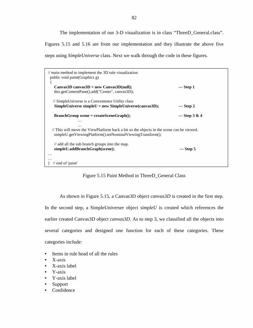
82
The implementation of our 3-D visualization is in class “ThreeD_General.class”.
Figures 5.15 and 5.16 are from our implementation and they illustrate the above five
steps using SimpleUniverse class. Next we walk through the code in these figures.
Figure 5.15 Paint Method in ThreeD_General Class
As shown in Figure 5.15, a Canvas3D object canvas3D is created in the first step.
In the second step, a SimpleUniverser object simpleU is created which references the
earlier created Canvas3D object canvas3D. As to step 3, we classified all the objects into
several categories and designed one function for each of these categories. These
categories include:
• Items in rule head of all the rules• X-axis• X-axis label• Y-axis• Y-axis label• Support• Confidence
// main method to implement the 3D rule visualization public void paint(Graphics g) { Canvas3D canvas3D = new Canvas3D(null); --- Step 1 this.getContentPane().add("Center", canvas3D);
// SimpleUniverse is a Convenience Utility class SimpleUniverse simpleU = new SimpleUniverse(canvas3D); --- Step 2
BranchGroup scene = createSceneGraph(); --- Step 3 & 4……
// This will move the ViewPlatform back a bit so the objects in the scene can be viewed. simpleU.getViewingPlatform().setNominalViewingTransform();
// add all the sub branch groups into the map. simpleU.addBranchGraph(scene); --- Step 5……} // end of 'paint'

83
• Support label• Confidence label• Items name.
The purpose of classify these categories is for the convenience of update our
visualization system. For example, if we want to change the color of support, we only
need to modify one function that is related to this category. These functions are
developed to create the objects we needed.
Figure 5.16 illustrates one of these functions createSceneGraph. This function is
used to create all the items in rule head of each rule. Each item is represented with a
small cube and all the cubes are displayed on a three-dimensional graph. The default of
the cube shows only one face. To show more than one face of the cube, we need to rotate
the cube. Rotation can be made about X-axis, Y-axis or Z-axis. The method rotX, rotY
and rotZ in class Transform3D are used to for this task. In order to rotate about two axes,
two different transformations should be specified for a single visual object. Figure 5.16
shows how to combine the two transformations to make a complex rotation.
After we specified the rotation, we began to retrieve the data from RULE table.
All the items in rule head of each rule are retrieved and stored in a Vector. Then a cube is
created for each item retrieved using the class ColorCube. The position of each cube in
the three-dimensional graph is set by the setTranslation method in Transform3D class.
The parameter of method setTranslation is a Vector3f object, which stores the position of
each cube in three-dimensional graph.
After all the cubes have been created, we compile these objects in the content
branch in step 4. Compiling the content branch converts it to a more efficient form, thus
this step is used for the optimization.

84
Figure 5.16 Content Branch for Items in the Rule Head of All Rules
public BranchGroup createSceneGraph() // create the items { // Create the root of the branch graph BranchGroup objRoot = new BranchGroup(); Appearance app = new Appearance();
TransformGroup objRotate = null; Transform3D transform = new Transform3D(); Transform3D transformZ = new Transform3D(); transform.rotX(Math.PI/6.0d); transformZ.rotZ(Math.PI/2.0d); // rotate to adjust the viewer’s color transform.mul(transformZ);
for(int i=0;i<rcount;i++)
{ Vector vCurHead = new Vector(); String TotalHead = vHead.elementAt(i).toString().trim(); StringTokenizer st = new StringTokenizer(TotalHead, ","); while (st.hasMoreTokens()) // add all items in the current rule head vCurHead.addElement(st.nextToken().trim()); // into the vCurHead
for(int j=0;j<vCurHead.size();j++) { int jPos=0; String CurHead = vCurHead.elementAt(j).toString().trim(); for(int w=0;w<vDisctHead.size();w++) { if(CurHead.equals(vDisctHead.elementAt(w).toString().trim())) { jPos = w; break; } } // end of ’for(w)’ // create ColorCube objects transform.setTranslation(new Vector3f( (float)(-1.0+i*0.1), (float)(-0.6+jPos*0.1), (float)(-1.2-jPos*0.1))); objRotate = new TransformGroup(transform); objRotate.setCapability(TransformGroup.ALLOW_TRANSFORM_WRITE); objRotate.setCapability(TransformGroup.ALLOW_TRANSFORM_READ); objRoot.addChild(objRotate); objRotate.addChild(new ColorCube(0.03)); } // end of inner ’for’ } // end of outer ’for’ // Let Java 3D perform optimizations on this scene graph. objRoot.compile(); --- Step 4
return objRoot; } // end of CreateSceneGraph method
85
As in rule table module, in the 3-D visualization module, all the operators that we
used for database access, such as ‘LIKE’, ‘IN’, ‘NOT’, ‘AND’, ‘OR’, ‘>’, etc, are
standard operators. As a consequence, using JDBC, all the operations in our visualization
tool are identical for any DBMS. No extra code is necessary for different DBMSs. So our
visualization tool is purely independent of specific DBMS.
86
CHAPTER 6CONCLUSION AND FUTURE WORK
6.1 Conclusion
We first discussed the architectures of JDBC application. Between 2-tier and 3-
tier architectures, 2-tier is chosen because no business logic is incorporated and hence
addition of a tier adds complexity without any gains for what we are trying to do. Next,
the advantages and disadvantages of two data mining architecture alternatives “Cache-
Mine” and “SQL-based” are analyzed.
We used association rule mining to compare these two architecture alternatives.
Intelligent Miner is chosen as the representative of “Cache-Mine” architecture. We
implemented three mining algorithms (K-Way Join, 2-Groupby, and Subquery) based
purely on SQL-92 and three ones (Vertical, GatherJoin, and GatherJoin Variant) based on
SQL-OR. We did some performance tests over DB2 for Intelligent Miner and our six
approaches using the different sized synthetic generated data sets. Based only on the
performance, Cache-Mine is better than SQL-based approach, but it needs additional
space to store the data in the local disk. In additional, SQL-based approach can utilize the
SQL capability provided by DBMS. But the Cache-Mine does not have this advantage.
Everything (including results) is stored in the local disk.
We implemented the mapping of intermediate rule table into the format that the
user can understand easily. A visualization module that includes rule table and 3-D

87
graphics was developed to help the user get the interested information easier through
sorting, and filtering functions.
Besides the performance, there are some more differences between Intelligent
Miner and our implementation:
• Intelligent Miner can use the data stored in flat file and DB2 database.
However, our software can access the data stored in multiple DBMS through
JDBC, such as DB2 and Oracle.
• Intelligent Miner can only use the data from one table. However, we can use
the data from multiple tables through join/union operation.
• In Intelligent Miner, “Transaction ID” and “Item” has to be a single field. But
we extend this ability to process multiple fields. The user can specify which
fields are used as “Transaction ID” and which fields are used as “Item”.
• Intelligent Miner uses Directed – Graph as the base of rule visualization
technique. As described in Chapter 4, it uses ‘item-item’ relationship so it
works well in the situation of few rules. However, our visualization module
uses ‘rule-item’ relationship so that it can display more rules at one time. In
additional, the rule sorting and filtering ability of our visualization module
gives the user more flexibility and efficiency in managing and understanding
the association rule.
• Intelligent Miner stores the results in the local disk as flat file. In our
implementation, we store the generated rules in the database. Once the rules
are stored in database, they can be easily handled because of the SQL
capabilities.
88
6.2 Contributions
In this thesis, we have addressed the following problems.
• Implement three SQL-92 approaches and three SQL-OR approaches using
Oracle stored procedures for association rule mining.
• Once the intermediate rule table is generated, map back to the final rule table
so that each item has a self-explain name
• Compare the performance of three SQL-92 approaches and three SQL-OR
approaches using different sized synthetically generated data sets.
• Conduct the scale-up experiments for our six approaches using different sized
synthetically generated data sets.
• Develop a visualization module using Java 3D to help the user manage and
understand the association rules.
• Compare our implementation with one of the commercial data mining tools
Intelligent Miner in various aspects, such as user interface, input/output, and
visualization.
6.3 Future Work
We have identified the following work for future research.
1. In our implementation, although we can access different DBMSs, the data
from only one DBMS (either DB2 or Oracle) are used for mining. We plan to
provide the user an interface to generate the input data set using the data from
all the databases the user specified and apply our mining algorithm to the
generated input data set.
89
2. We plan to extend the existing mining operations. In this thesis, we
implemented “association rule” using a series of SQL queries. The next step is
to explore the possibility of implement the other mining operations, such as
classification and clustering using SQL queries.
3. As to the visualization module, we plan to add more function such as zoom in,
zoom out so that the user can have more control over the rules.
4. We plan to explore the possibility of developing some of the operations for
association rule as the operators of the database. These operations include
SaveTid(), which is used to create the tid list for each item, and CountAndk(),
which is used to get the number of common elements from k CLOBs, etc. If
these operations can be part of the database operators, it will make mining for
an association rule easier. Further, we can explore the possibility of
developing the whole association rule mining as one operator of the database
so that the user only needs to give the DBMS the input table. If this happens,
there is no clear boundary of issuing a basic query command and a data
mining operation to the user.

90
APPENDIXASSOCIATION RULE MINING EXAMPLE USING KWAY JOIN
This appendix lists one example input data set, the intermediate candidate sets Cx,
the intermediate frequent item set Fx, and the final association rules using KWay Join
approach with minimum support of 50%, and minimum confidence of 50%.
Input Data Set
We use a small input data set that has 4 transactions (different TID denotes
different transactions). Each transaction has 2 or 3 items. The total number of records is
12. Table A-1 shows the items of all the transactions. For example, for the transaction
where TID=100, the items are “Milk, Eggs, Bread”.
Table A-1 Example of Input Data Set
TID ITEM100 Milk100 Eggs100 Bread200 Sugar200 Eggs200 Cake300 Milk300 Sugar300 Eggs300 Cake400 Sugar400 Cake

91
In order to convert the string format of item to integer format, we generate a
“description” table for each item. We can do this by scanning the input data set. For each
distinct item, we assign it a distinct number. Table A-2 shows the description table of the
example input data set. It has 5 distinct items.
Table A-2 Example of Description Table
ITEM NUMBER DESCRIPTION1 Milk2 Sugar3 Eggs4 Bread5 Cake
The “Mapping” process is to convert all the TID and ITEM from string format to
integer format. Based on Table A-1 and Table A-2, the final input data set is generated
and stored in database as Table A-3.
Table A-3 TIDITEM Table
TID ITEM100 1100 3100 4200 2200 3200 5300 1300 2300 3300 5400 2400 5
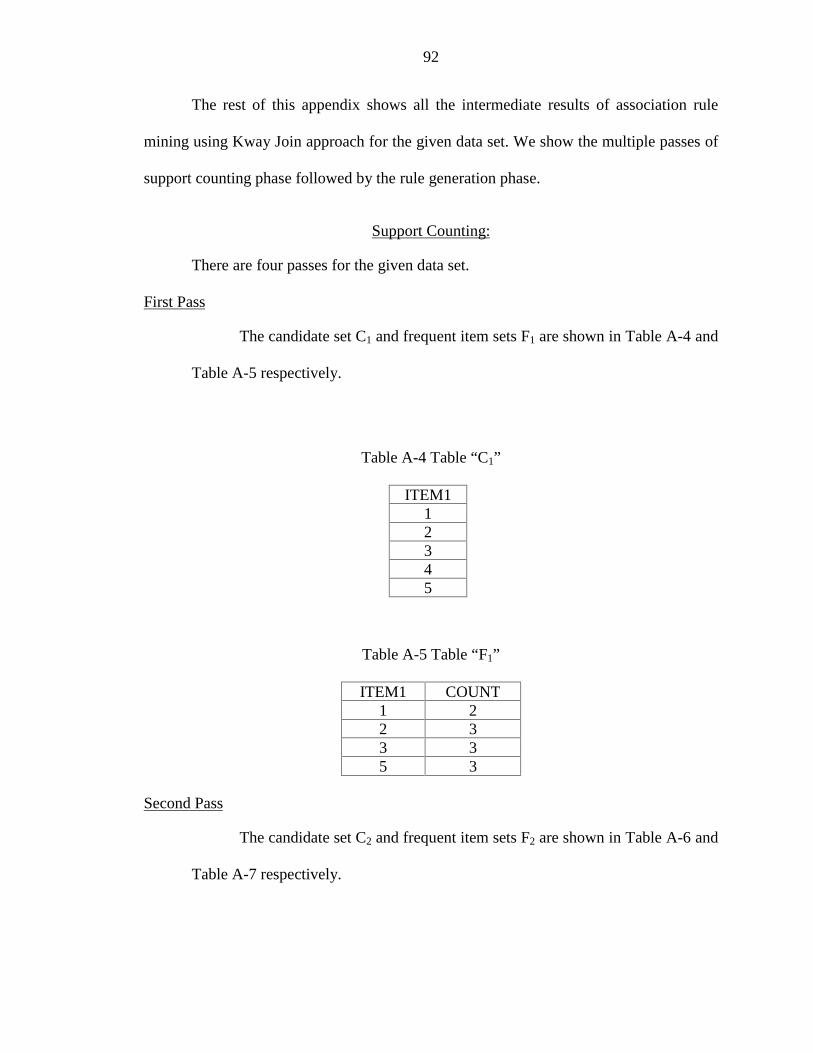
92
The rest of this appendix shows all the intermediate results of association rule
mining using Kway Join approach for the given data set. We show the multiple passes of
support counting phase followed by the rule generation phase.
Support Counting:
There are four passes for the given data set.
First Pass
The candidate set C1 and frequent item sets F1 are shown in Table A-4 and
Table A-5 respectively.
Table A-4 Table “C1”
ITEM112345
Table A-5 Table “F1”
ITEM1 COUNT1 22 33 35 3
Second Pass
The candidate set C2 and frequent item sets F2 are shown in Table A-6 and
Table A-7 respectively.

93
Table A-6 Table “C2”
ITEM1 ITEM21 21 31 41 52 32 42 53 43 54 5
Table A-7 Table “F2”
ITEM1 ITEM2 COUNT1 3 22 3 22 5 33 5 2
Third Pass
The candidate set C3 and frequent item sets F3 are shown in Table A-8 and
Table A-9 respectively.
Table A-8 Table “C3”
ITEM1 ITEM2 ITEM31 2 31 2 51 3 41 3 52 3 5
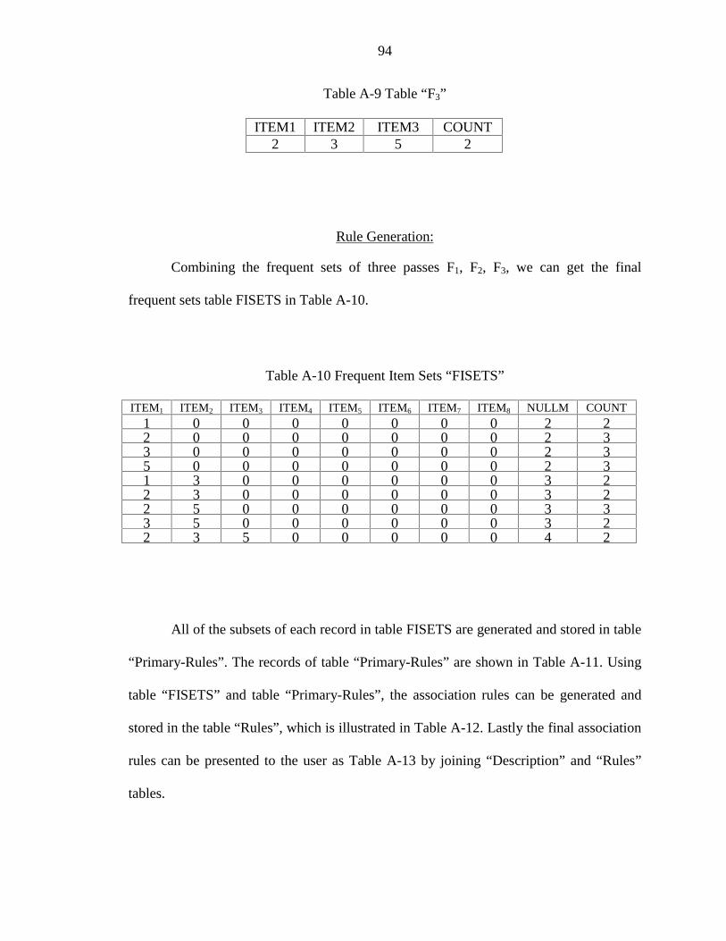
94
Table A-9 Table “F3”
ITEM1 ITEM2 ITEM3 COUNT2 3 5 2
Rule Generation:
Combining the frequent sets of three passes F1, F2, F3, we can get the final
frequent sets table FISETS in Table A-10.
Table A-10 Frequent Item Sets “FISETS”
ITEM1 ITEM2 ITEM3 ITEM4 ITEM5 ITEM6 ITEM7 ITEM8 NULLM COUNT1 0 0 0 0 0 0 0 2 22 0 0 0 0 0 0 0 2 33 0 0 0 0 0 0 0 2 35 0 0 0 0 0 0 0 2 31 3 0 0 0 0 0 0 3 22 3 0 0 0 0 0 0 3 22 5 0 0 0 0 0 0 3 33 5 0 0 0 0 0 0 3 22 3 5 0 0 0 0 0 4 2
All of the subsets of each record in table FISETS are generated and stored in table
“Primary-Rules”. The records of table “Primary-Rules” are shown in Table A-11. Using
table “FISETS” and table “Primary-Rules”, the association rules can be generated and
stored in the table “Rules”, which is illustrated in Table A-12. Lastly the final association
rules can be presented to the user as Table A-13 by joining “Description” and “Rules”
tables.
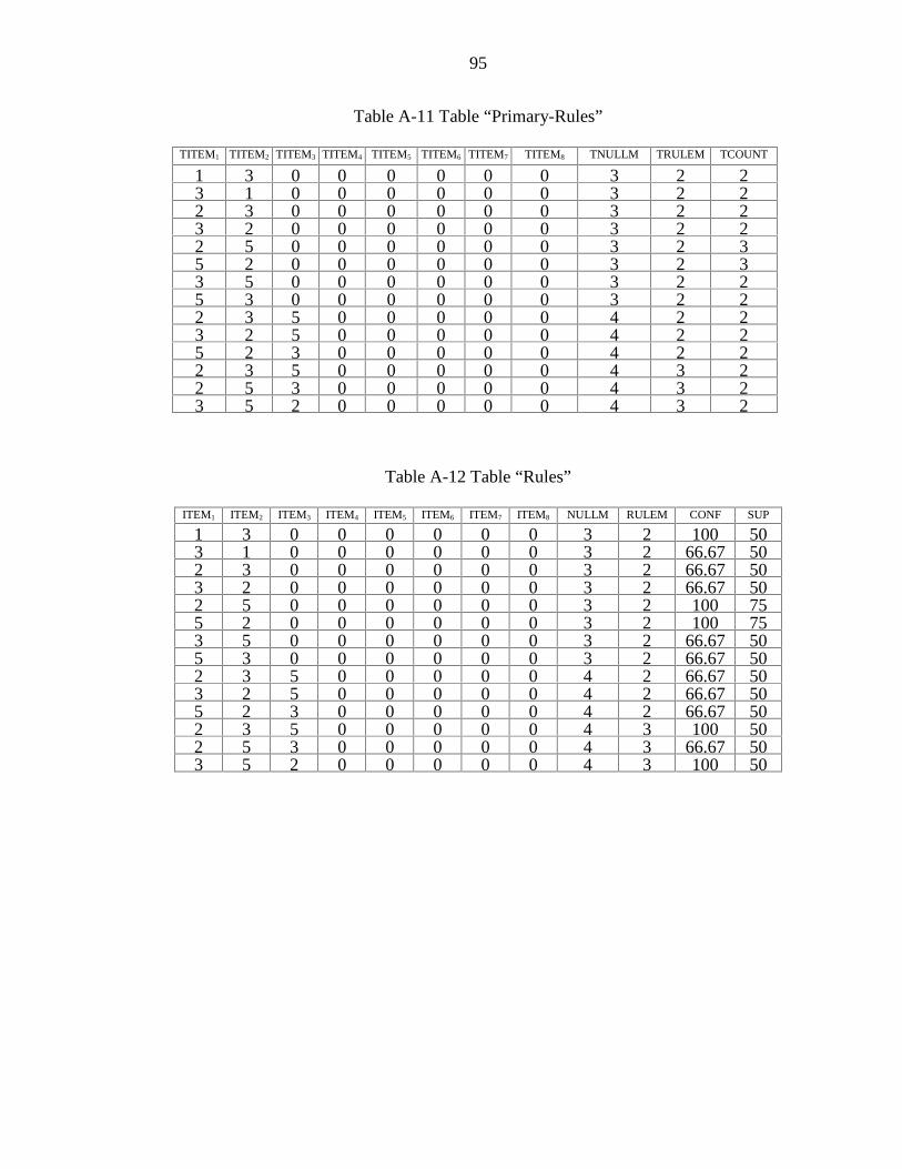
95
Table A-11 Table “Primary-Rules”
TITEM1 TITEM2 TITEM3 TITEM4 TITEM5 TITEM6 TITEM7 TITEM8 TNULLM TRULEM TCOUNT
1 3 0 0 0 0 0 0 3 2 23 1 0 0 0 0 0 0 3 2 22 3 0 0 0 0 0 0 3 2 23 2 0 0 0 0 0 0 3 2 22 5 0 0 0 0 0 0 3 2 35 2 0 0 0 0 0 0 3 2 33 5 0 0 0 0 0 0 3 2 25 3 0 0 0 0 0 0 3 2 22 3 5 0 0 0 0 0 4 2 23 2 5 0 0 0 0 0 4 2 25 2 3 0 0 0 0 0 4 2 22 3 5 0 0 0 0 0 4 3 22 5 3 0 0 0 0 0 4 3 23 5 2 0 0 0 0 0 4 3 2
Table A-12 Table “Rules”
ITEM1 ITEM2 ITEM3 ITEM4 ITEM5 ITEM6 ITEM7 ITEM8 NULLM RULEM CONF SUP
1 3 0 0 0 0 0 0 3 2 100 503 1 0 0 0 0 0 0 3 2 66.67 502 3 0 0 0 0 0 0 3 2 66.67 503 2 0 0 0 0 0 0 3 2 66.67 502 5 0 0 0 0 0 0 3 2 100 755 2 0 0 0 0 0 0 3 2 100 753 5 0 0 0 0 0 0 3 2 66.67 505 3 0 0 0 0 0 0 3 2 66.67 502 3 5 0 0 0 0 0 4 2 66.67 503 2 5 0 0 0 0 0 4 2 66.67 505 2 3 0 0 0 0 0 4 2 66.67 502 3 5 0 0 0 0 0 4 3 100 502 5 3 0 0 0 0 0 4 3 66.67 503 5 2 0 0 0 0 0 4 3 100 50

96
Table A-13 Final “Association Rules”
Rule Head Symbol Rule Body Confidence(%) Support(%)Milk => Eggs 100 50Eggs => Milk 67 50Sugar => Eggs 67 50Eggs => Sugar 67 50Sugar => Cake 100 75Cake => Sugar 100 75Eggs => Cake 67 50Cake => Eggs 67 50Sugar => Eggs, Cake 67 50Eggs => Sugar, Cake 67 50Cake => Sugar, Eggs 67 50Sugar, => Cake 100 50Sugar, => Eggs 67 50Eggs, Cake => Sugar 100 50
97
LIST OF REFERENCES
[AGR1993] Agrawal R., Imielinski T., and Swami S., Mining Association rulesbetween sets of items in large databases, Proc. of the ACM SIGMODConference on Management of Data, Washington, DC, May 1993.
[AGR1994] Agrawal R., Srikant R., Fast Algorithms for Mining Association Rules,Proc. of the 20th Int’l Conference on Very Large Database, Santiago,Chile, September 1994.
[AGR1995a] Agrawal R., Psaila G., Active Data Mining, Proc. of the 1st Int'lConference on Knowledge Discovery and Data Mining, Montreal, August1995.
[AGR1995b] Agrawal R., Psaila G., Wimmers E., and Zait M., Querying shapes ofhistories, Proceedings of the 21st International Conference on Very LargeDatabases, Zurich, Switzerland, September 1995.
[AGR1995c] Agrawal R., Srikant R., Mining Sequential Patterns, Proc. of the Int’lConference on Data Engineering, Taipei, Taiwan, 1995.
[AGR1998] Agrawal R., Gehrke J., Gunopulos D., Raghavan P., Automatic SubspaceClustering of High Dimensional Data for Data Mining Applications, Proc.of the ACM SIGMOD Int’l Conference on Management of Data, Seattle,Washington, June 1998.
[BEC1998] Becker B. G., Visualizing Decision Table Classifiers, Proceedings ofInformation Visualization, Research Triangle Park, North Carolina,October 1998.
[CHA1995] Chakravarthy S., Krishnaprasad V., Tamizuddin Z., and Badani R. H.,ECA Rule Integration into an OODBMS: Architecture andImplementaion, 11th International Conference on Data Engineering,Taipei, Taiwan, March 1995.
[CHA1998] Chamberlin D., A Complete Guide to DB2 Universal Database, MorganKaufmann Publishers, Inc, San Mateo, California, 1998.
[DUD2000] Dudgikar M., A Layered Approach for Mining Association Rules overRelational DBMS, Master’s thesis, University of Florida, Gainesville,2000.
98
[GER1998] Gershon N., Eick S. G., and Card S., Information Visualization, ACMInteractions, vol. 5, no. 2, pp. 9-15, March/April 1998.
[GRI1995] Grinstein G. and Thuraisingham D., Data Mining and Data Visualization,Database Issues for Data Visualization, Proceedings of IEEEVisualization’95 Workshop, Phoenix, Arizona, October 1995.
[HET1998] Hetzler B., Harris W. M., Havre S., and Whiteny P., Visualizing the FullSpectrum of Document Relationships, Proceedings of the FifthInternational Society for Knowledge Organization Conference, SanFrancisco, California, April 1998.
[IBM2000] IBM, http://www.software.ibm.com/data/iminer, January 2000.
[KEI1996] Keim D. A., and Kriegel H. P., Visualization Techniques for MiningLarge Databases: A Comparison, IEEE Transactions on Knowledge andData Engineering, vol. 8, no. 6, pp. 923-938, December 1996.
[LEN1997] Lent B., Agrawal R., and Srikant R., Discovering Trends in TextDatabases, Proc. of the 3rd Int’l Conference on Knowledge Discovery inDatabases and Data Mining, Newport Beach, California, August 1997.
[MEH1996] Metha M., Rissanen J., and Agrawal R., SLIQ: A Fast Scalable Classifierfor Data Mining, Proc. of the Fifth Int’l Conference on ExtendingDatabase Technology, Avignon, France, March 1996.
[ORA1997] Oracle 8 Application Developer’s Guide, Chapter 10: Using Proceduresand Packages, Oracle, Belmont, California, 1997.
[SGI2000] SGI, http://www.sgi.com/software/mineset/index.html, February 2000.
[SHA1996] Shafer J. C., Agrawal R., and Mehta M., A Scalable Parallel Classifier forData Mining, Proc. of the 22th Int’l Conference on Very Large Databases,Mumbai (Bombay), India, September 1996.
[SUN1999] Sun Microsystems, http://java.sun.com/products/java-media/3D/collateral,July 1999.
[SUN2000] Sun Microsystems, http://java.sun.com/products/jdk/1.2/docs/guide/jdbc/,January 2000.
[THO1998] Thomas S., Architectures and Optimizations for Integrating Data MiningAlgorithms with Database Systems, Ph.D. dissertation, University ofFlorida, Gainesville, 1998.

99
[WON1999] Wong P. C., Whitney P., Thomas J., Visualizing Association Rules forText Mining, Proceedings of the 1999 IEEE Symposium on InformationVisualization, San Francisco, California, October 1999.
100
BIOGRAPHICAL SKETCH
Hongen Zhang was born on October 27, 1972, in Xinchang county, Zhejiang
province, P.R. China. He received his bachelor’s degree in forest genetics from Zhejiang
Forest College in June 1994. After his graduation, he was admitted to Bejing Forest
University in September 1994 and received his Master of Science degree in forest
genetics from Beijing Forest University in June 1997.
He joined the Department of Computer and Information Science and Engineering
at the University of Florida in spring 1999. He has worked as a graduate research
assistant in the Database Systems Research and Development Center of the department.
He worked with Dr. Sharma Chakravarthy to study the different SQL approaches of
association rules. He will receive his Master of Science degree in August 2000.