Minimum Specific Energy and Transcritical Flow in …375793/UQ375793_OA.pdf · 61 equation for steady flow that always predicts dh/dx→∞ at ... O., and CHANSON, H. (2016). "Minimum

CASTRO-ORGAZ, O., and CHANSON, H. (2016). "Minimum Specific Energy and Transcritical Flow in Unsteady Open-Channel Flow." Journal of Irrigation and Drainage Engineering, ASCE, Vol. 142, No. 1, Paper 04015030, 12 pages (DOI: 10.1061/(ASCE)IR.1943-4774.0000926) (ISSN 0733-9437 [Print]; ISSN: 1943-4774 [online]).

1

Minimum Specific Energy and Transcritical Flow in unsteady Open 1

Channel Flow 2

3

Oscar Castro-Orgaz1 and Hubert Chanson2 4

5

Abstract: The study and computation of free surface flows is of paramount importance in 6

hydraulic and irrigation engineering. These flows are computed using mass and momentum 7

conservation equations whose solutions exhibit special features depending on whether the local 8

Froude number is below or above unity, thereby resulting in wave propagation in the up- and 9

downstream directions or only in the downstream direction, respectively. This dynamic condition is 10

referred in the literature to as critical flow and is fundamental to the study of unsteady flows. 11

Critical flow is also defined as the state at which the specific energy and momentum reach a 12

minimum, based on steady-state computations, and it is further asserted that the backwater equation 13

gives infinite free surface slopes at control sections. So far, these statements were not demonstrated 14

within the context of an unsteady flow analysis, to be conducted herein for the first time. It is 15

demonstrated that the effects of unsteadiness break down critical flow as a generalized open channel 16

flow concept, and correct interpretations of critical flow, free surface slopes at controls, minimum 17

specific energy and momentum are given within the context of general unsteady flow motion in this 18

educational paper. 19

20

DOI: 21

22

CE Database subject headings: Critical flow condition, Open channel, Transcritical flow, Water 23

discharge measurement, Unsteady Flow, Weir 24

______________________________________________________________________ 25


2

1Professor of Hydraulic Engineering, University of Cordoba, Spain, Campus Rabanales, Leonardo 26

Da Vinci building, E-14071, Cordoba, Spain. E-Mail: [email protected], [email protected] 27

(author for correspondence) 28

29

2Professor in Hydraulic Engineering, The University of Queensland, School of Civil Engineering, 30

Brisbane QLD 4072, Australia. Email: [email protected]. 31


3

Introduction 32

Shallow open channel flows occurs in a wide range of engineering problems including irrigation 33

canals, dam spillways, or drainage channels. These flows are mathematically computed using 34

vertically-integrated conservation equations of mass and momentum assuming that the pressure 35

distribution is hydrostatic (Yen 1973, 1975; Liggett 1993, Montes 1998). Free surface flows are 36

classified as sub- or supercritical depending on whether the local Froude number F is above or 37

below the threshold value F=1, respectively. The limiting value F=1 is a dynamic criterion defining 38

critical flow as the flow condition for which the mean flow velocity exactly equals the celerity of an 39

elementary gravity wave (Liggett 1993, 1994). Critical flow is defined by the following 40

simultaneous proprieties in the literature (Chow 1959, Henderson 1966, Montes 1998, Hager 1999, 41

Jain 2001, Sturm 2001, Chanson 2004, Chaudhry 2008): (i) Specific energy is minimum 42

(Bakhmeteff 1932, Jaeger 1949), (ii) Mean flow velocity equals the celerity of a small gravity wave 43

(Stoker 1957, Liggett 1993), (iii) Specific force reaches a minimum (Jaeger 1949, Chow 1959), (iv) 44

Water surface slope is infinite in the steady backwater equation (Bélanger 1828, Henderson 1966), 45

and (v) Discharge per unit width is maximum, as used in the design of MEL culverts (Apelt 1983, 46

Chanson 2004). These properties may be also extended to non-hydrostatic pressure fields (Chanson 47

2006). The five conditions stated are linked in the literature as simultaneous conditions defining 48

critical flow as a unique dynamic state. However, a number of critiques may be raised: 49

(i) Critical depth in a rectangular channel is hc=(q2/g)1/3, with q as the unit discharge. This depth 50

originates by setting dE/dh=0 in the specific energy definition E[=h+q2/(2gh2)], or dS/dh=0 in the 51

specific force or specific momentum expression S[=h2/2+q2/(gh)]. The minimum values Emin and 52

Smin corresponding to hc are obtained assuming that the flow is steady (Jaeger 1949). However, 53

critical flow defined as F=1 is obtained by setting the slope of the unsteady backward characteristic 54

curve dx/dt=U−(gh)1/2=0 (Liggett 1993), from which U=(gh)1/2, where F=U/(gh)1/2 is the Froude 55

number, U=q/h is the mean flow velocity, x is the longitudinal coordinate, t is time and h the water 56


4

depth. This results from an unsteady flow analysis, in contradiction to the steady flow analysis 57

while computing the extremes of E and S. 58

(ii) Unsteady computation of transcritical flows using the Saint-Venant equations lacks from infinite 59

free surface slopes away from shocks (Toro 2002). This is not in agreement with the backwater 60

equation for steady flow that always predicts dh/dx→∞ at critical flow. This is a paradox, given that 61

the backwater equation is a simplification for steady state of the unsteady Saint-Venant equations 62

(Chanson 2004), from which both should be identical. 63

These observations indicate that the effect of unsteadiness on critical flow was so far not 64

investigated. This research was designed to fill in this gap, given that critical flow is one of the most 65

important concepts on which the theory of open channel flow relies. The first objective of this 66

research is to verify the computation of the steady transcritical water surface profiles over variable 67

topography, with weir flow as a representative test case, using the gradually-varied flow equation 68

assisted by the singular point method to remove the indetermination at the critical point, given the 69

lack of general acceptance of this method in the hydraulics community. Unsteady flow 70

computations using a finite volume model are conducted to compute the asymptotic steady flow 71

profile starting from another steady state. The asymptotic unsteady flow computations are then used 72

to track if a singular point is formed in the computational domain as steady state is approached. 73

Unsteady flow results are further used to compute numerically the water surface slope at the 74

channel control to its comparison with the corresponding steady state solution using L'Hopital's 75

rule. This analysis will serve to decide if the backwater equation is associated with singularities that 76

can be handled using L'Hopital's rule or, in contrast, with an infinity free surface slope, as normally 77

assumed in the literature. 78

The second objective of this work is to investigate if critical flow is a unique dynamic state in 79

transient flows. Following Liggett (1993) the definition of critical flow should specify the point at 80

which the equations of motion (both steady and unsteady) are singular. He further indicated that the 81


5

critical depth could be defined by minimizing the specific energy, but such a definition would not 82

expose the singularities in the equations of motion, and, therefore, would have little use. However, 83

no proof or discussion of these differences was given so far. As pointed out above the definition of 84

critical flow using the continuity and momentum equations in unsteady flow [dx/dt=0, with q=q(x, 85

t) and h=h(x, t)] is not coherent with the steady definition of critical flow as the state for which the 86

specific energy becomes a minimum [dE/dh=0, with q=const and h=h(x)]. This is in close 87

agreement with the statements of Liggett (1993). This point is especially important given that all 88

hydraulic books, so far available and used for teaching and research in open channel hydraulics, 89

implicitly assume that both conditions are equivalent, without any analytical or numerical proof. 90

Thus, general unsteady flow computations of transcritical flow over a weir are conducted in this 91

work to compute the evolution of E(x, t), F(x, t) and S(x, t) in the x-t computational domain. The 92

aim of these computations is to investigate if the point F=1 (dx/dt=0) generally agrees with the 93

points where E and S reach a minimum value. Further, critical flow defined as the maximum 94

discharge for a given specific energy permits to define head-discharge relationships used for 95

discharge measurements purposes (Bos 1976, Chanson 2004). Computation of the relationship 96

between discharge and specific energy at a weir crest during unsteady flow will reveal if the 97

maximum discharge condition applies for water discharge measurement. This study therefore will 98

reveal if critical flow can be defined as a unique flow state in transient flows, or if the effect of 99

unsteadiness is to break down critical flow as a generalized open channel flow concept. 100

101

Steady flow 102

Governing equations 103

Steady-state shallow water open channel flows are computed using the gradually-varied flow 104

equation (Chow 1959, Henderson 1966, Jain 2001, Sturm 2001, Chanson 2004) 105

106


6

2

d

d 1o fS Sh

x

F (1) 107

108

Here So=channel slope and Sf=friction slope. For the sake of simplicity a rectangular cross-section 109

of constant width is considered in this work. Equation (1) is a first order differential equation that 110

must be solved subjected to one boundary condition that is a known flow depth for a given 111

discharge (Chaudhry 2008). The specific energy E in open channel flow is defined as (Bakhmeteff 112

1912, 1932; Chow 1959, Henderson 1966) 113

114

2 2

22 2

U qE h h

g gh (2) 115

116

It is well known that the minimum specific energy dE/dh=0 is reached at the critical depth 117

hc=(q2/g)1/3 (i.e. Henderson 1966), where the specific momentum S=h2/2+q2/(gh) also reaches a 118

minimum value (Jaeger 1949). Inserting this depth into the definition of F yields U=(gh)1/2 and 119

dh/dx→∞ in Eq. (1). The consequence is that it is routinely stated in the literature that the 120

gradually-varied flow equation breaks down at the critical flow condition. In an attempt to justify 121

that from a physical standpoint, one argument is that near the critical depth the pressure is non-122

hydrostatic and, therefore, Eq. (1) is invalid. However, the mathematical validity of Eq. (1) at a 123

critical point is different from the physical correctness of the gradually-varied flow theory if 124

pressure is not hydrostatic, as detailed in the next section. The Belanger-Böss theorem (Jaeger 1949, 125

Montes 1998) states the equivalence of dE/dh=0 for q=const and dq/dh=0 for E=const. Thus, the 126

discharge becomes a maximum for the given specific energy head under critical flow in steady 127

flows. 128

129


7

Singular point method 130

An important case of transcritical open channel flow is the passage from sub- (F<1) to supercritical 131

(F>1) flow over variable topography, typically over a weir (Fig. 1). Let zb(x) be the bed profile and 132

assume that the flow is frictionless, i.e. Sf=0, so that Eq. (1) reduces to 133

134

2

d

d 1

bzh xx

F

(3) 135

136

An infinite free surface slope is not observed experimentally in transcritical flow over a weir (Blau 137

1963, Wilkinson 1974, Hager 1985, Chanson and Montes 1998, Chanson 2006). If F=1, then Eq. 138

(3) must equal the indeterminate identity dh/dx=0/0. This automatically fixes the critical point at the 139

weir crest ∂zb/∂x=0 (Hager 1985, 1999). However, the value of dh/dx remains unknown, although 140

the slope is definitely not infinite. This singularity is removed by applying L’Hospital's rule to 141

Eq. (3), resulting in (Massé 1938, Escoffier 1958) 142

143

1 22

2

d

d 3c b

c

h zh

x x

(4) 144

145

This technique to remove flow depth gradients of the kind 0/0 on the shallow-water steady state 146

equations is known as the singular point method. It originates from the work of Poincaré (1881) on 147

ODE equations, and was applied to open channel transition flow problems by Massé (1938), 148

Escoffier (1958), Iwasa (1958), Wilson (1969) and Chen and Dracos (1996). However, this method 149

is rarely accepted by open channel flow workers given that the argument still prevails that Eq. (1) is 150

invalid for h=hc given the existence of a non-hydrostatic pressure distribution. As discussed above 151

the gradually-varied flow model is mathematically valid at the critical depth, but it is physically 152


8

inaccurate if the flow curvature is high (Montes 1998). The singular point method is rarely 153

explained in open channel flow books, with Chow (1959) and Montes (1998) as exceptions. 154

However, mathematical books often describe it for general application in engineering (i.e. von 155

Kármán and Biot 1940). Given the lack of general acceptance of the singular point method for the 156

steady, gradually-varied flow equation, its validity will be assessed using general unsteady flow 157

computations to produce an asymptotic steady state. This will permit to track if a singular point is 158

asymptotically formed in the computational domain as a steady state is approached. 159

160

Unsteady flow 161

Governing equations 162

One-dimensional unsteady shallow water flows are described by the Saint-Venant equations, 163

written in conservative vector form as (Vreugdenhil 1994, Chaudhry 2008) 164

165

t x

U F

S (5) 166

167

Here U is the vector of conserved variables, F is the flux vector and S the source term vector, given 168

by 169

170

2 2

0

; ;1

2b

f

hUh

zgh ShU hU gh

x

U F S (6) 171

172

Again, Eq. (5) is based on the assumption of hydrostatic pressure. It can be solved to compute the 173

transcritical flow profile over variable topography subjected to suitable initial and boundary 174

conditions. A steady flow profile can be simulated using unsteady flow computations until an 175


9

equilibrium state is obtained as given by the corresponding boundary and initial conditions. Modern 176

shock-capturing methods like the finite volume method apply to produce transcritical flow profiles 177

over variable topography without any additional special care or technique as the flow passes across 178

the point h=hc. This unsteady flow computation of a free surface profile can be therefore compared 179

with the steady state computation based on Eq. (3) assisted by Eq. (4) to remove the singularity at 180

the critical point. The unsteady flow computations can also be used to compute the asymptotic 181

steady free surface slope at the critical point and, then, to compare the numerical estimates with the 182

analytical steady-state solution given by Eq. (4). Further, during the transient flow, the functions 183

E=E(x, t), S=S(x, t) and F=F(x, t) can be tracked to detail their evolution as functions of both time 184

and space. It will serve to highlight if steady-state definitions of critical flow, i.e. E=Emin and 185

S=Smin, apply to unsteady flow motion and agree with the unsteady critical flow condition dx/dt=0 186

(or F=1). The numerical computations used in this work are described in the next section. 187

188

Numerical method of solution 189

Among the possible methods of solution for Eq. (5) the finite volume method was selected. Shock 190

capturing finite volume solutions using the Godunov upwind method assisted by robust Riemann 191

solvers (approximate or exact) are well established today as accurate solutions of shallow-water 192

flows (Toro 2002, LeVeque 2002). The integral form of Eq. (5) over a control volume is (Toro 193

1997, 2002) 194

195

d d dA

At

U

n F S (7) 196

197

where Ω is the control volume, A the cell boundary area and n the outward unit vector normal to A. 198

Choosing a quadrilateral control volume in the x-t plane, the conservative Eq. (7) reads (Toro 2002) 199


10

200

11 2 1 2

n ni i i i i

tt

x

U U F F S (8) 201

202

Here n refers to the time level, i is the cell index in the x-direction, and Fi+1/2 is the numerical flux 203

crossing the interface between cells i and i+1 (Fig.2a). Source terms Si and the fluxes Fi+1/2 are 204

evaluated at a suitable time level depending on the specific method. In this work the MUSCL-205

Hancock method is used (Toro 1997, 2002), which is second-order accurate in both space and time. 206

Specific aspects of the method are detailed below. 207

208

Reconstruction of solution 209

The solution process starts with the cell-averaged values of conserved variables at time level n, Uin. 210

To obtain second order accuracy in space, a piecewise linear reconstruction is made within each cell 211

(Toro 2002) (Fig. 2a). Linear slopes resulting from the reconstructed solution must be limited to 212

avoid spurious oscillations near discontinuities. Let letters L and R denote the reconstructed 213

variables at the left and right sides of a cell interface, so that the resulting values of U at each of its 214

sides are with 1 2i

and 3 2i

as diagonal limiter matrices (Toro 2002) 215

216

1 2 1 2 1 2 3 21 1 2 1

1 1;

2 2i i i i

L n n n R n n ni i i i i i

U U U U U U U U (9) 217

218

A Minmod limiter is used in all computations presented herein. Further, Eq. (9) implies that the 219

water depths at each time level n are reconstructed. This technique is denoted as the depth-gradient 220

method (Aureli et al. 2008). Another option is to use the auxiliary vector Q=(h+zb, Uh) instead of 221

U=(h, Uh). The reason is that reconstruction using water depths may lead to non-physical flows 222


11

over variable topography under static conditions, an issue that is fully resolved if the reconstruction 223

is based on the water surface elevation zs=h+zb (Zhou et al. 2001) using a suitable bottom source 224

term discretization. However, as pointed out by Aureli et al. (2008), the surface gradient method 225

may lead to oscillations and unphysical depths (even negative) for shallow supercritical flows. In 226

contrast, the depth-gradient method is more stable and robust for bore front tracking. During this 227

work both methods were applied to transcritical flow over weirs; it was found that the surface 228

gradient method leads in some cases to unstable results in the tailwater supercritical portion of the 229

weir face, in agreement with the results of Aureli et al. (2008). In contrast, the results using the 230

depth-gradient method were found accurate enough, and, thus, results based on that technique are 231

presented herein. 232

233

Numerical flux 234

The computation of the numerical flux Fi+1/2 at each interface requires knowledge of boundary-235

extrapolated values of variables at the left and right sides of the interface 1 2i

L

U and

1 2i

R

U . In the 236

MUSCL-Hancock method an additional step is added rendering a non-conservative evolution of 237

boundary extrapolated values 1 2i

L

U and

1 2i

R

U at interface i+1/2 over half the time step, to regain 238

second order accuracy in time as (Fig. 2b) 239

240

1 2 1 2 1 2 1 2

1 2 1 2 3 2 1 2 1

;2 2

2 2

i i i i

i i i i

L L L Ri

R R L Ri

t t

xt t

x

U U F U F U S

U U F U F U S

(10) 241

242

With these evolved boundary extrapolated variables 1 2i

L

U and 1 2i

R

U defining states L and R the 243

numerical flux is computed using the HLL approximate Riemann solver (Fig.2c) as (Toro 2002) 244


12

245

1/2

if 0

, if 0

if 0

LL

R L L R R L R Li L R

R LR

R

SS S S S

S SS S

S

F

F F U UF

F

(11) 246

247

Here FL and FR are the fluxes computed at states L and R. Robust wave speeds estimates SL and SR 248

(Fig.2d) are given by (Toro 2002) 249

250

;L L L L R R R RS U a q S U a q (12) 251

252

where a=(gh)1/2, and qK(K=L, R) is 253

254

1 2

* **2

*

( )1

2

1

K

KK

K

K

h h hh h

q h

h h

(13) 255

256

The flow depth at the start region of the Riemann problem at each interface h* is (Toro 2002) 257

258

2

*

1 1 1

2 4L R L Rh a a U Ug

(14) 259

260

Time stepping 261

For stability in time of the explicit scheme, the Courant-Friedrichs-Lewy number CFL must be less 262

than unity (Toro 1997, 2002). For selection of the time step, CFL was fixed to 0.9 in this work and 263

Δt was determined at time level n using the equation 264


13

265

1 2

max n ni i

xt

U gh

CFL (15) 266

267

Here ∆t and ∆x are the step sizes in the x and t axes, respectively. 268

269

Source terms 270

The computation of shallow-water flow over variable topography must be conducted using a well-271

balanced scheme. It implies that once a discretization is applied to the source terms, the time 272

evolution of the conserved variables must reach a stable steady state Uin+1=Ui

n if afforded by the 273

boundary conditions. That is, the asymptotic steady state version of Eq. (8) 274

275

1 2 1 2i i ix F F S 0 (16) 276

277

may be regarded as an identity that is verified only if the discretization of S is correctly done. For 278

the MUSCL-Hancock scheme using the surface gradient method a well-balanced discretization of 279

the bottom slope term is (Zhou et al. 2001) 280

281

1 2 1 2

2

L Rbi bib i i

z zz h hh

x x

(17) 282

283

It implies that the bed profile is linearly distributed within a cell, with a mean bed elevation for cell 284

i given by 285

286


14

1 2 1 2

2bi bi

bi

z zz

(18) 287

288

For the depth-gradient method the model would give unphysical flows under static conditions, 289

however. Static tests resulted in discharges of less than 10−5 m2/s for the weirs simulated, so that the 290

model was considered accurate enough. In the numerical literature passing a static test (q=0) is 291

considered an index of good predictions of steady-state solutions. However, it does not imply, in 292

general, that the identity given by Eq. (16) is verified for any discharge q≠0. So, in turn, an 293

unsteady numerical model must be checked and compared with steady-state solutions, as done in 294

this work. 295

296

Initial conditions 297

The test cases considered in this work are weir flows of parabolic and Gaussian shapes. Specific 298

details of each weir tested are given in the results section. An initial steady free surface profile over 299

the weir, for which q=constant and h=h(x) is known, must be prescribed to initiate unsteady 300

computations. In this work Eq. (1) was used to produce an initial free surface profile for a low 301

discharge over the weir, i.e. q=0.01 m2/s. The profile was numerically computed using the 4th order 302

Runge-Kutta method (Chaudhry 2008). Computations started at the crest section where h=hc. At 303

this section Eq. (4) was implemented in the Runge-Kutta solver, and the corresponding sub- and 304

supercritical branches of the water surface profile were computed in the up- and downstream 305

directions, respectively. 306

307

Boundary conditions 308

For transcritical flow over a weir one boundary condition must be prescribed at the subcritical 309

section on the upstream weir side, whereas at the supercritical outlet section no boundary conditions 310


15

need to be prescribed. The inlet boundary condition is given by an instantaneous rise in the 311

discharge, which is kept constant during all the transient flow. Unknown values of conserved 312

variables at boundary sections are then computed using ghost cells by extrapolation of values at 313

adjacent interior cells (LeVeque 2002). The use of ghost cells is a common technique in finite 314

volume methods and gives results that are enough accurate (LeVeque 2002, Ying et al. 2004). 315

316

Alternative solution 317

In this work the MUSCL-Hancock method was further compared with the one-sided upwind finite 318

volume method of Ying et al. (2004). In this model the Saint-Venant equations are recast with zs as 319

the free surface elevation in the form 320

321

2

0

; ;s

f

h hUz

gh ShU hUx

U F S (19) 322

323

With this formulation the model equations automatically pass the still water numerical test (Ying et 324

al. 2004). The gradient ∂zs/∂x is computed based on the Courant number, as given by Ying et al. 325

(2004), and the numerical flux is 326

327

21/2

ni k

ni i k

ni k

q

q

h

F (20) 328

329

Here k=0 if qi and qi+1>0, k=1 if qi and qi+1<0, and k=1/2 for any other case, where i+1/2 means in 330

that case average values at i and i+1 grid points. 331

332


16

Accuracy of Saint Venant equations for variable topography 333

For steady, frictionless flow over a weir, Eq. (1) or Eqs. (5) are equivalent to conservation of the 334

total energy head H as 335

336

2

22b

qH z h

gh (21) 337

338

This equation gives smooth mathematical solutions for transcritical flow over a weir and is 339

consistent with the formation of steady singular points asymptotically during an unsteady flow. 340

However, these issues are related to the mathematical possibility of computing transcritical flows 341

using gradually-varied flow models, but not to the physical accuracy or correctness of the theory 342

itself. One aspect widely criticised in the water discharge measurement literature is that for weir 343

flows the pressure is non-hydrostatic, making Eq. (21) invalid (Blau 1963, Bos 1976, Hager 1985, 344

Montes 1994, Chanson 2006, Castro-Orgaz 2013). In contrast, numerical literature widely uses the 345

transcritical flow over a weir as a performance test of numerical schemes for solving the Saint-346

Venant equations. Thus, their validity for variable bed topography is examined herein. Matthew 347

(1991), using Picard’s iteration technique, obtained with the sub-index indicating ordinary 348

differentiation with respect to x the second order equation for potential free surface flow as 349

350

222

2

21

2 3xx x

b bxx bx

hh hqH z h hz z

gh

(22) 351

352

This is a second order differential equation describing the flow depth profile h=h(x). For its 353

solution, an initial value of H is adopted and the upstream boundary flow depth is computed as the 354

subcritical root of Eq. (21). The free surface slope is set to zero at that section. Using these 355


17

boundary conditions Eq. (22) is then integrated using the 4th-order Runge-Kutta method. The 356

upstream head must be iterated until the supercritical root of Eq. (21) is reached at the tailwater 357

section. 358

359

Results 360

Steady water surface profiles 361

The steady water surface profile over a weir of bed shape zb=0.2−0.01x2(m) was computed for a 362

target discharge of q=0.18 m2/s using the MUSCL-Hancock method, and the results are shown in 363

Fig. 3a. This particular weir is widely used to test unsteady numerical models (i.e. Zhou et al. 2001, 364

Ying et al. 2004). In this case ∆x=0.05 m and CFL=0.9 were used. The results presented in the 365

figure correspond to a simulation time of t=50 s. The steady water surface profile computed using 366

Eqs. (3) and (4) is presented in the same figure, showing excellent agreement with the finite volume 367

computation. This suggests that the application of the singular point method correctly produces the 368

transcritical flow profile over variable topography. As further observed the discharge is conserved 369

with good accuracy by the unsteady flow model. The same computations were conducted in Fig. 3b 370

using the one-sided upwind finite volume method, with results almost identical (the two profiles 371

deviates in the 3rd decimal position) to those using the MUSCL-Hancock method, justifying the use 372

of the depth-gradient method in the present work. 373

374

Water surface slope at critical point 375

The unsteady flow model was used to compute numerically the water surface slope at the weir crest 376

at any instant of time to second order accuracy as 377

378

1 1d

d 2i i

c

h hh

x x

(23) 379


18

380

Computational simulations until reaching a steady state over the weir were conducted for varying 381

discharges at the weir inlet. The unsteady numerical results at t=50 s obtained from Eq. (23) are 382

plotted in Fig. 4 together with the analytical steady-state Eq. (4). Both results almost perfectly 383

match, thereby indicating that the unsteady flow over a weir produces a singular point 384

asymptotically in the crest section as the steady state is approached. It demonstrates that the singular 385

point method is a correct mathematical tool permitting to remove indeterminations in the 386

computational domain as the flow passes from sub- to supercritical. This technique permits to 387

mimic with a steady-state computation what shock-capturing unsteady computations automatically 388

do. Experimental data of Wilkinson (1974) for steady flow over cylindrical weirs are plotted in Fig. 389

4, indicating the accuracy of the Saint-Venant theory in predicting the free surface slope at the 390

control section up to −hczbxx=0.15. Following Wilkinson (1974) the accuracy of water surface slope 391

computations using the singular point method is restricted to the limit −hczbxx≈0.25, given the 392

curvilinear flow over the crest domain. The accuracy of the theory is further exploited below by 393

considering the existence of a non-hydrostatic pressure. 394

395

Accuracy of Saint-Venant theory 396

Figure 5 contains the experimental data of Sivakumaran et al. (1983) for a Gaussian hump of profile 397

zb=20exp[−0.5(x/24)2] (cm) for two test cases. The computed Saint-Venant solution using the finite 398

volume method is presented for both cases and compared in the same figures with the non-399

hydrostatic steady flow computations using Eq. (22). The clear departure between the two for the 400

test case of Fig. 5a (Emin/R=0.516, q=0.111 m2/s) indicates that the effect of the vertical acceleration 401

as the flow passes from sub- to supercritical is significant, so that the Saint-Venant theory does not 402

apply despite the flow is shallow. For the test case of Fig. 5b (Emin/R=0.253, q=0.0359 m2/s) the 403

deviation of results is small, but still appreciable. This computation sets as limit of application of 404


19

the Saint-Venant theory roughly −hczbxx=(2/3)(E/R)≈0.168, or simply 0.15, in agreement with 405

previous results of Fig. 4. No explicit limit of application of the Saint-Venant theory for flow over 406

variable topography appears to be previously available. 407

408

Water wave celerity, minimum specific energy and flow momentum in unsteady flow 409

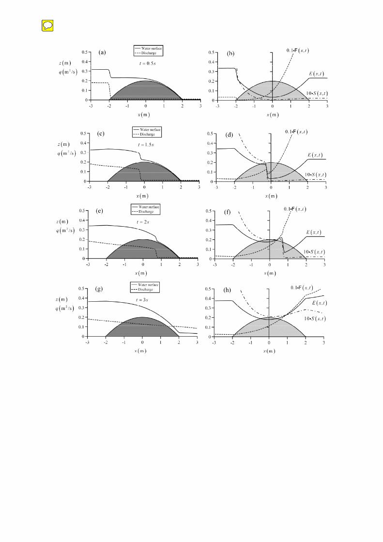
The unsteady flow motion corresponding to the steady water surface profiles of Fig. 3a is detailed 410

in Fig. 6. Figures 6 (a), (c), (e) and (g) show water and discharge profiles at computational times 411

t=0.5, 1.5, 2 and 3 s, respectively. The functions E(x, t), F(x, t) and S(x, t) are plotted for the same 412

times in Fig.6 (b), (d), (f) and (h). Note firstly that a shock is formed given the sudden rise in 413

discharge (Fig.6a), and a smooth unsteady flow without discontinuities follows at t=3 s (Fig.6g). As 414

observed, E(x, t), F(x, t) and S(x, t) are discontinuous as the shock propagates, with left-side 415

variables affected by unsteady motion and right-side variables corresponding to the initial steady-416

state conditions. The values of E(x, t), F(x, t) and S(x, t) at crest vicinity are detailed in Fig. 7 for the 417

previous simulation times. At time t=0.5 s the shock has not reached yet the crest (Fig.6a) so E(x, t), 418

F(x, t) and S(x, t) at the weir zone are those of the initial steady flow (Fig.7a). At time t=1.5 s the 419

discontinuity associated with the shock is near the crest (Fig. 7b), but the crest is not yet affected by 420

the transient flow. At time t=2 s the shock front is roughly at x=0.9 m, so the flow variables near the 421

crest are effected by unsteadiness. Note that the section of Emin is clearly not at the crest, and further 422

different from the section where F=1. There is not a minimum in the S function at this instant of 423

time. Computations at t=3 s indicate that the entire computational domain is free from 424

discontinuities in the solution (Fig. 6g), so all sections are affected by unsteadiness. The results of 425

Fig. 7d are most revealing. The specific energy E=Emin occurs at the crest section (x=0) but the 426

condition F=1 is reached at a section x<0. There is a minimum of specific momentum S=Smin, but it 427

is at a section x>0. These results clearly reveal that the effect of unsteadiness provokes non-428

uniqueness of the critical flow concept, i.e. each critical flow definition is related to a different 429


20

depth located at a different channel section, so that the traditional results are of no use here. At 430

t=50 s the flow is steady and all definitions of critical flow converge with a single control section at 431

the weir crest (Fig. 7e). 432

433

Unstable transcritical flow profiles 434

In the singular point theory Eq. (4) gives two roots (positive/negative), each associated with a 435

different transcritical flow profile (Chow 1959, Montes 1998). The negative sign correspond to the 436

transition from sub- to supercritical flow, already used herein in the former computations. It remains 437

to investigate if the inverse transition from super- to subcritical flow is likely to be of practical 438

significance. Kabiri-Samani et al. (2014) demonstrated experimentally that the transition from 439

super- to subcritical flow without a hydraulic jump is possible. Both experiments and steady-state 440

singular point theory, therefore, support this transitional flow profile as a valid solution. The 441

purpose of this section is to investigate if this transition profile is a rubust and stable profile relative 442

to unsteady flow perturbations (as is the transition from sub- to supercritical flow). The steady-state 443

computations for this kind of transitional flow proceed with no problem just taking the positive root 444

in Eq. (4). This was done for the weir test of Fig. 3, where the water surface profiles for the initial 445

discharge, and the target discharge of 0.18 m2/s, are plotted in Fig. 8a. The question is if the 446

unsteady flow computations produce the target steady profile of this transitional flow type, starting 447

from another transition profile corresponding to the initial steady flow. For this test case, as the inlet 448

flow is supercritical, two boundary conditions, depth and discharge, must be prescribed. These are 449

taken from the target steady flow profile. At the outlet subcritical section only the depth is specified, 450

whereas the discharge is computed using ghost cells. The evolution of the unsteady flow motion is 451

depicted in Fig. 8, where two shocks are formed (Fig. 8b and c) until they intersect at t=1.5 s 452

(Fig.8d), thereby leading to a single shock propagating toward the inlet section (Fig. 8e and f). If the 453

boundary conditions at the inlet section are changed to permit the flow passage, a whole subcritical 454


21

flow profile is finally formed over the weir once steady state is reached. The same behaviour was 455

obtained using small variations of the target steady-state over the initial steady flow profile. It was 456

impossible to obtain the transcritical flow profile from F>1 to F<1 as the result of asymptotic 457

unsteady flow computations. In contrast, the reverse transitional flow (i.e. Fig. 3) was always stable 458

and convergent in unsteady flow computations. 459

460

Rating curve in unsteady flow 461

In steady flows, critical flow defined as the maximum discharge for a given E yields the rating 462

curve (Montes 1998, Chanson 2004) 463

464

3 2

1 232

3c cq gE

(24) 465

466

For weir flow Ec and qc are specific energy and discharge at the crest section, respectively. This is a 467

basic steady-state rating curve assumed to apply for water discharge measurement purposes (Bos 468

1976), or to characterize outflow structures of dams (Montes 1998) (with correction coefficients as 469

for non-hydrostatic pressure if the flow curvature is high). To test its accuracy during unsteady 470

flows the values of Ec(t) and qc(t) for the weir flow problem shown in Fig. 3 were computed. 471

Equation (24) and the unsteady flow results are shown in Fig. 9. The first unsteady point 472

corresponding to the initial steady flow (q=0.01 m2/s) lies on Eq. (24). As soon as the shock waves 473

passes the crest section, and the flow there becomes unsteady, the unsteady crest rating curve 474

deviates from Eq. (24), implying, physically, that the value of qc is not a maximum for Ec. As the 475

unsteady flow tends to the new steady state corresponding to q=0.18 m2/s, the unsteady data point 476

tends to lie on Eq. (24). Lines of ±5% of deviation in q relative to Eq. (24) are plotted in the same 477

figure as doted lines. Note that a significant part of the unsteady rating curve is outside this domain, 478


22

rendering Eq. (24) inaccurate for water discharge measurements purposes during the entire unsteady 479

flow motion. Unsteady flow data of Chanson and Wang (2013) yielded a rating curve for a V-notch 480

weir close to steady flow, despite the highly-rapidly flow motion in their experiments. However, the 481

problem investigated herein is different, involving a shock wave propagating over the weir crest 482

(Fig. 6c and e). The flow just behind the shock induced a strong unsteadiness effect on the weir 483

crest conditions (i.e. Fig. 6e for t=2 s). Thus, the flow profile over the weir crest is continuous 484

(∂h/∂x is finite) with a strong effect of unsteadiness on both qc and Ec induced by the shock wave 485

propagating in the tailwater weir face. At time t=3 s (Fig. 6g) there are no shocks in the 486

computational domain and the unsteady rating curve is within ±5% of deviation for the steady 487

rating curve (Fig. 9). 488

489

Discussion 490

Saint-Venant equations produce realistic free-surface profile solutions across the critical depth 491

using shock capturing numerical methods. The computation of a steady flow profile using an 492

unsteady flow computation produces a solution that automatically crosses the critical depth. This 493

unsteady flow computation is performed without any further special treatment at the critical point, 494

as the unsteady computation does not suffer from any mathematical indetermination. However, the 495

steady backwater equation has an indetermination at critical flow conditions that must be resolved 496

using L'Hopital's rule. The unsteady computation produces such singular point asymptotically as the 497

steady state is approached. 498

The steady free surface slope for the transition from sub- to supercritical flow computed from the 499

unsteady flow model perfectly matches the analytical solution for steady flow obtained using 500

L´Hospital's rule. It means that the unsteady flow model produces automatically such a critical point 501

gradient in the computational domain to pass across the critical depth. The Saint-Venant equations 502


23

are mathematically valid at the critical depth over variable topography. However, this model is 503

physically inaccurate if the flow curvature is high, with the threshold value of −hczbxx=0.15. 504

During a transient flow the positions of the points corresponding to E=Emin, S=Smin and F=1 are 505

different, and none is located at the weir crest. Once a steady flow is reached all definitions of 506

critical flow converge, with a unique control section at the weir crest. Thus, the time variable 507

produces non-uniqueness of the critical depth concept, with 3 different critical points in the 508

computational domain, each consistent with a definition of critical flow. The relevant definition for 509

unsteady flow is U=(gh)1/2 (for a rectangular channel), which is coherent with momentum 510

conservation and the singularity of the equations of motion, as suggested by Liggett (1993) without 511

proof. It means that the minimum specific energy is a steady-state concept, a point so far not 512

revealed in the literature, to the Authors' knowledge. Thus, the notion of critical flow as defined 513

from the specific energy minimum has little use in unsteady flow, but is a fundamental tool for 514

steady flows. In addition to the numerical results presented herein, a mathematical proof of 515

divergence between the conditions U=(gh)1/2 and E=Emin is given in the Appendix. 516

Starting unsteady flow computations with a transitional profile from F<1 to F>1 results in a new 517

stable transcritical flow profile after applying a perturbation at the inlet section in the form of a 518

discharge pulse. The same type of computation was conducted for the inverse transcritical flow 519

profile from F>1 to F<1, that is also theoretically possible within the singular point theory. 520

However, starting with this kind of steady transcritical flow profile and inducing perturbations 521

compatible with a new transitional profile from F>1 to F<1 (corresponding to a different steady 522

discharge) provokes unsteady flow profiles that do not result in a new transcritical flow profile 523

(from F>1 to F<1) as the steady flow condition is reached. Thus, the transition from super- to 524

subcritical flow over variable topography without a hydraulic jump is an unstable steady flow 525

profile relative to small unsteady flow perturbations. Possibly, this flow profile is generated using 526


24

very delicate adjustments of boundary conditions, but the present results indicate that this is not 527

likely to be a natural profile in real life conditions. 528

A weir crest is a discharge meter in steady flow where the rating curve is given by the maximum 529

discharge principle. During unsteady flow the relationship between E and q at the weir crest does 530

not follow the steady rating curve, thereby indicating that it is not a control section. Physically, it 531

means that if a discharge equation is defined based on the crest section then the discharge 532

coefficient and the ratio of crest depth to specific energy depend on time, and not constant values as 533

obtained in the classical steady-state analysis. From a practical standpoint this may have severe 534

implications, given that deviations of the real unsteady rating curve from the steady rating curve 535

may not be acceptable for water discharge measurement purposes. Thus, the major finding is that 536

Eq. (24) is never verified exactly in unsteady flow over a weir. As long as there are shocks in any 537

point of the computational domain downstream from the weir crest, the unsteadiness affect is 538

strong, and deviations of the unsteady rating curve from Eq. (24) are unacceptable. However, if the 539

instantaneous water surface profile is free from shocks deviations of the unsteady rating curve from 540

the critical depth rating curve are acceptable. 541

542

Conclusions 543

Unsteady computations of transcritical flow over variable bed topography were conducted using 544

weir flow as a representative case. Comparison of asymptotic unsteady flow profiles with steady 545

flow backwater computations indicates that the Saint-Venant equations produce a singular point 546

during the transient flow to cross critical points. This states that the singular point method is a 547

steady technique permitting to mathematically resolve the existence of these indeterminations, 548

which, in turn, are automatically computed with unsteady flow models. This demonstrates the 549

general validity of the singular point method and that the steady backwater equation is 550

mathematically valid at a critical point. However, although mathematically valid, the outcome of 551


25

the gradually-varied flow model is accurate only if the flow curvature in the vicinity of the critical 552

depth is small. 553

Unsteady numerical flow computations reveal that the section isolated from water waves 554

[U=(gh)1/2] is generally different from the sections where the specific energy and the specific 555

momentum reach minimum values. An analytical proof of the divergence of results is also given. 556

This leads to the conclusion that the only relevant definition of critical flow for both unsteady and 557

steady flow is F=U(x, t)/[gh(x, t)]1/2=1, that exhibits singularities in the equations of motion. 558

Consequently, the minimum specific energy and force are steady flow concepts of little use in 559

unsteady flow, although they are important tools for steady flow computations. 560

Computation of the relation between the discharge and specific energy at the weir crest during 561

unsteady flow revealed that the maximum discharge principle is not verified. Thus, use of crest 562

sections as discharge meters during unsteady flows needs to be done with caution, given that the 563

effect of unsteadiness may induce appreciable errors, that are, however, acceptable if the flow is 564

free from shocks. 565

This work was designed as an educational piece of work from which is concluded that the general 566

definition of critical flow implies a section where the flow is isolated from water waves (valid for 567

both unsteady and steady flows), as stated by Liggett (1993). The specific energy is a powerful 568

steady state concept, with a minimum value coincident with the definition of critical flow 569

originating from the equations of motion, if these are detailed to steady flow. Thus, minimum 570

specific energy and momentum should henceforth not used to define critical flow, but rather quoted 571

as particular cases where the simplification of critical flow to steady state regain an additional 572

physical meaning. 573

574

Acknowledgements 575


26

The Authors are very much indebted to Dr. Sergio Montes, University of Hobart, Tasmania, for his 576

advice on this research. The first Author is further greateful to Dr. L. Mateos, IAS-CSIC, for his 577

comments at several stages of this research work. This work was supported by the Spanish project 578

CTM2013-45666-R, Ministerio de Economía y Competitividad and by the Australian Research 579

Council (Grant DP120100481). 580

APPENDIX: Minimum specific energy and water wave celerity in unsteady flow 581

The specific energy is a function E=E(h, q), where both h and q are functions of (x, t). The total 582

variation of E is generally given by 583

584

d d dE E

E h qh q

(A1) 585

586

Further, the partial differentials of E are with Eq. (2) 587

588

2

3 21 ,

E q E q

h gh q gh

(A2) 589

590

Now, q and h vary in the (x, t) plane according to 591

592

d d d , d d dq q h h

q x t h x tx t x t

(A3) 593

594

Combining Eqs. (A1)-(A3) results in 595

596

2

3 2d 1 d d d d

q h h q q qE x t x t

gh x t gh x t

(A4) 597


27

598

The derivative dE/dh is thus given by the general equation 599

600

2d d d d d

1d d dt d d

E U t h x h U t q x q

h gh h x t gh h x t t

(A5) 601

602

Based on Eq. (A5) it is demonstrated that if dx/dt=0, that further implies F=U/(gh)1/2=1, does not 603

results in an extreme of the specific energy dE/dh=0 in unsteady flow, given that the term ∂q/∂t0. 604

605

Notation 606

The following symbols are used in this paper: 607

A=area of finite volume (m2) 608

a=shallow-water wave celerity=(gh)1/2 (m/s) 609

CFL= Courant-Friedrichs-Lewy number (-) 610

E = specific energy head (m) 611

F = Froude number (-) 612

F = vector of fluxes (m2/s, m3/s2) 613

g = gravity acceleration (m/s2) 614

H = total energy head (m) 615

h = flow depth measured vertically (m) 616

h*=intermediate flow depth in Riemann problem (m) 617

hc = critical depth for parallel-streamlined flow (m)=(q2/g)1/3 618

i = cell index in x-axis (-) 619

k = index (-) 620

n = node index in t-axis (-) 621


28

q = unit discharge (m2/s) 622

Q = alternative vector of conserved variables (m, m2/s) 623

qL, qR = auxiliary variables (-) 624

R =crest radius of curvature (m) 625

Sf = friction slope (-) 626

So = channel bottom slope (-) 627

S = specific force (or momentum) (m2) 628

SL, SR = slope of characteristics lines (negative and positive) in Riemann problem (-) 629

S = vector of source terms (m/s, m2/s2) 630

t = time (s) 631

U = mean flow velocity (m/s) = q/h 632

U = vector of conserved variables (m, m2/s) 633

x = horizontal distance (m) 634

zs = free surface elevation (m) 635

zb = channel bottom elevation (m) 636

+, − = limiter matrices (-) 637

Ω = control volume (m3) 638

Subscripts 639

min=minimum value 640

c=crest section 641

L=left state in Riemann problem 642

R=right state in Riemann problem 643

644

References 645


29

Apelt, C.J. (1983). Hydraulics of minimum energy culverts and bridge waterways. Australian Civil 646

Engrg Trans., I.E.Aust. CE25(2), 89-95. 647

Aureli, F., Maranzoni, A., Mignosa, P., Ziveri, C. (2008). A weighted surface-depth gradient 648

method for the numerical integration of the 2D shallow water equations with topography. 649

Advances in Water Resources 31(7), 962–974. 650

Bakhmeteff, B.A. (1912). O neravnomernom wwijenii jidkosti v otkrytom rusle (St Petersburg, 651

Russia [in Russian]. (Varied flow in open channels) 652

Bakhmeteff, B.A. (1932). Hydraulics of open channels. McGraw-Hill, New York. 653

Bélanger, J.B. (1828). Essai sur la solution numérique de quelques problèmes relatifs au 654

mouvement permanent des eaux courantes. Carilian-Goeury, Paris [in French]. (On the 655

numerical solution of some steady water flow problems) 656

Bos, M.G. (1976). Discharge measurement structures. Publ. 20, Intl. Inst. for Land Reclamation 657

(ILRI), Wageningen NL. 658

Blau, E. (1963). Der Abfluss und die hydraulische Energieverteilung über einer parabelförmigen 659

Wehrschwelle (Distributions of discharge and energy over a parabolic-shaped weir). 660

Mitteilungen der Forschungsanstalt für Schiffahrt, Wasser- und Grundbau, Berlin, Heft 7, 5-72 661

[in German]. 662

Castro-Orgaz, O. (2013). Potential flow solution for open channel flows and weir crest overflows. J. 663

Irrig. Drain. Engng. 139(7), 551-559. 664

Chanson, H., Montes, J.S. (1998). Overflow characteristics of circular weirs: effects of inflow 665

conditions. J. Irrig. Drain. Engng. 124(3), 152-162. 666

Chanson, H. (2004). The hydraulics of open channel flows: An introduction. Butterworth-667

Heinemann, Oxford, UK. 668

Chanson, H. (2006). Minimum specific energy and critical flow conditions in open channels. J. 669

Irrig. Drain. Engng. 132(5), 498-502. 670


30

Chanson, H., Wang, H. (2013). Unsteady discharge calibration of a large V-notch weir. Flow 671

measurement and Instrumentation 29, 19-24. 672

Chaudhry, M.H. (2008). Open-channel flow, 2nd ed. Springer, New York. 673

Chen, J., Dracos, T. (1996). Water surface slope at critical controls in open channel flow. J. Hydr. 674

Res. 34(4), 517-536. 675

Chow, V.T. (1959). Open channel hydraulics. McGraw-Hill, New York. 676

Escoffier, F.F. (1958). Transition profiles in nonuniform channels. Trans. ASCE 123, 43-56. 677

Henderson, F.M. (1966). Open channel flow. MacMillan Co., New York. 678

Hager, W.H. (1985). Critical flow condition in open channel hydraulics. Acta Mechanica 54(3-4), 679

157-179. 680

Hager, W.H. (1999). Wastewater hydraulics: theory and practice. Springer, Berlin. 681

Iwasa, Y. (1958). Hydraulic significance of transitional behaviours of flows in channel transitions 682

and controls. Memoires of the Faculty of Engineerig, Kyoto University, 20(4), 237-276. 683

Jaeger, C. (1949). Technische Hydraulik (Technical hydraulics). Birkhäuser, Basel [in German]. 684

Jain, S.C. (2001). Open channel flow. John Wiley & Sons, New York. 685

Kabiri-Samani, A., Hossein Rabiei, M., Safavi, H., Borghei, S.M. (2014). Experimental–analytical 686

investigation of super- to subcritical flow transition without a hydraulic jump. J. Hydraul. Res. 687

52(1), 129-136. 688

LeVeque, R.J. (2002). Finite volume methods for hyperbolic problems. Cambridge Univ. Press, 689

New York. 690

Liggett, J.A. (1993). Critical depth, velocity profile and averaging. J. Irrig. Drain. Engng. 119(2), 691

416-422. 692

Liggett, J.A. (1994). Fluid mechanics. McGraw-Hill, New York. 693


31

Massé, P. (1938). Ressaut et ligne d´eau dans les cours à pente variable (Hydraulic jump and free 694

surface profile in channels of variable slope). Rev. Gén. Hydr. 4(19), 7-11; 4(20), 61-64 in 695

French. 696

Matthew, G.D. (1991). Higher order one-dimensional equations of potential flow in open channels. 697

Proc. ICE 91(3), 187-201. 698

Montes, J.S. (1994). Potential flow solution to the 2D transition from mild to steep slope. J. Hydr. 699

Engng. 120(5), 601-621. 700

Montes, J.S. (1998). Hydraulics of open channel flow. ASCE, Reston, Va. 701

Poincaré, H. (1881). Mémoire sur les courbes définies par une équation différentielle (Memoir on 702

the defined curves of a partial differential equation). J. Math. Pures Appl. 7, 375-422 in 703

French. 704

Sivakumaran, N.S., Tingsanchali, T., Hosking, R.J. (1983). Steady shallow flow over curved beds. 705

J. Fluid Mech. 128, 469-487. 706

Stoker, J.J. (1957). Water waves: The mathematical theory with applications. Interscience 707

Publishers, New York. 708

Sturm, T.W. (2001). Open channel hydraulics. McGraw-Hill, New York. 709

Toro, E.F. (1997). Riemann solvers and numerical methods for fluid dynamics. Springer, London. 710

Toro, E.F. (2002). Shock-capturing methods for free-surface shallow flows. John Wiley & Sons, 711

Singapore. 712

von Kármán, T., Biot, M.A. (1940). Mathematical methods in engineering: an introduction to 713

mathematical treatment of engineering problems. McGraw-Hill, New York. 714

Vreugdenhil, C.B. (1994). Numerical methods for shallow water flow. Kluwer, Norwell MA. 715

Wilkinson, D.L. (1974). Free surface slopes at controls in channel flow. J. Hydr. Div., ASCE, 716

100(8), 1107-1117. 717


32

Wilson, E.H. (1969). Surface profiles in non-prismatic rectangular channels. Water Power 21(11), 718

438-443. 719

Yen, B.C. (1973). Open-channel flow equations revisited. J. Engng. Mech. Div. ASCE 99(5), 979-720

1009. 721

Yen, B.C. (1975). Further study on open-channel flow equations. SFB 80/T/49. Universität 722

Karlsruhe. 723

Ying, X., Khan, A., Wang, S. (2004). Upwind conservative scheme for the Saint Venant equations. 724

J. Hydraul. Eng. 130(10), 977–987. 725

Zhou, J.G., Causon, D.M., Mingham, C.G., Ingram, D.M. (2001). The surface gradient method for 726

the treatment of source terms in the shallow water equations. J. Comput Phys. 168(1), 1-25. 727

728


33

List of figures 729

730

Figure 1. Transcritical flow profile over variable topography: formation of steady singular point 731

Figure 2. Finite volume solution using MUSCL-Hancock method: (a) Linear reconstruction within each cell, (b) 732

evolution of boundary extrapolated values, HLL Riemann solver for each interface in (c) (U-x) plane, (d) (x-t) plane 733

Figure 3. Finite volume solution of flow over parabolic weir by (a) MUSCL-Hancock scheme, (b) one-sided upwind 734

scheme 735

Figure 4. Water surface slope at weir control section obtained from MUSCL-Hancock finite-volume model, analytical 736

steady result [Eq.(4)] and experiments (Wilkinson 1974) 737

Figure 5. Accuracy of shallow-water, gradually-varied flow theory over weir for Emin/R= (a) 0.516, (b) 0.253 738

Figure 6. Propagation of positive wave and temporal evolution of variables F, E and 739

Figure 7. Variables F, E and S at crest zone during transient flow 740

Figure 8. Unstable transcritical flow profile from super- to subcritical flow during unsteady flow 741

Figure 9 Comparison of steady rating curve with results of unsteady flow computation 742

e2hchans

Sticky Note

CASTRO-ORGAZ, O., and CHANSON, H. (2016). "Minimum Specific Energy and Transcritical Flow in Unsteady Open-Channel Flow." Journal of Irrigation and Drainage Engineering, ASCE, Vol. 142, No. 1, Paper 04015030, 12 pages (DOI: 10.1061/(ASCE)IR.1943-4774.0000926) (ISSN 0733-9437 [Print]; ISSN: 1943-4774 [online]). Figure 1

e2hchans

Sticky Note


e2hchans

Sticky Note


e2hchans

Sticky Note


e2hchans

Sticky Note


e2hchans

Sticky Note


e2hchans

Sticky Note


e2hchans

Sticky Note


e2hchans

Sticky Note


Documents

Minimum Specific Energy and Transcritical Flow in …375793/UQ375793_OA.pdf · 61 equation for steady flow that always predicts dh/dx→∞ at ... O., and CHANSON, H. (2016). "Minimum