Minimization of the positional errors for an accurate determinationof the kinematic parameters of a rigid-body system with miniature

inertial sensors

Jurij Zumera, Janko Slavica, Miha Boltezara,∗

aUniversity of Ljubljana, Faculty of Mechanical Engineering, Askerceva 6, SI-1000 Ljubljana, SloveniaCite as:

Zumer, Jurij, Janko Slavic, and Miha Boltezar. ”Minimization of the positional errors for an accuratedetermination of the kinematic parameters of a rigid-body system with miniature inertial sensors.” Mechanism

and Machine Theory 81 (2014): 193-208.DOI: 10.1016/j.mechmachtheory.2014.07.008

http://www.sciencedirect.com/science/article/pii/S0094114X14001840

Abstract

This paper presents an approach to minimize and control the error of the kinematic parame-ters of the space-constraint rigid-body system by using inertial micro-electro-mechanical sensors(MEMS). We analyze the error propagation when the kinematic joint constraints are observed fora sensor-fusion update in the kinematic model because of the uncertain position of the inertial sen-sors. The minimization of the errors of the kinematic parameters comes from applying multipleinertial units on every rigid body with the controlled input positional error between each inertialunit. The analytical approach proposes the inclusion of the position vectors from the inertial unitsto the kinematical joints into the state vector that consists of the observed kinematical and sensorparameters. A Kalman-filtering procedure is used to observe the state vector and, additionally,the adaptive estimation of the position vectors from the inertial units to the kinematic joints orconstraints is presented in order to achieve the optimum performance of the filter. The analyticalapproach is experimentally validated on a pendulum mechanism, where the improved performanceof the proposed approach is confirmed.

Keywords: rigid-body system, kinematic joint, accelerometer, gyroscope, sensor fusion, errorminimization

1. Introduction

Control over the kinematics of a rigid-body system, such as an industrial mechanism, is essen-tial in engineering practice. On the one hand, the kinematic parameters of the observed system canbe analytically defined, but this procedure might be time consuming because of the complexity of

∗Corresponding authorEmail address: miha.boltezar@fs.uni-lj.si (Miha Boltezar)

Preprint submitted to Elsevier August 29, 2014

the system, and furthermore, obtaining information about the exact external forces over time isusually not straightforward if the system is not kinematically driven. On the other hand, the exper-imental observation and control of the kinematic parameters is a strongly competitive approach,especially if the parameters must be observed or controlled at a later stage. These experimentalprocedures are possible with inertial MEMS sensors, which in the past decade have begun to offeran alternative to traditional inertial sensors, or other appropriate devices, such as encoders and op-tical systems. The advantages of MEMS are a small weight and size and an attractive price, whiletheir disadvantages relate to their long-term stability and accuracy, which become crucial duringan integration procedure over time.

To control the long-term precision of experimentally defined kinematic parameters researchershave used aiding systems to update the inertial parameters. The fusion of different systems largelydepends on the observed application. In the field of biomechanics Roetenberg [1, 2] and Schep-ers [3, 4] presented extensive research on combining the magnetic and inertial principle for anorientation determination of the human body. In industrial environments the use of the magneticprinciple might be critical because of the interference with local magnetic fields or because of theferromagnetic materials of the mechanisms, despite the proposed calibration procedures. Further-more, the use of the magnetic and inertial principles shows reduced precision when the humanbody is exposed to increased translational and rotational accelerations because of the loosely-coupled constraints between the parts of the human body and the environment, as was shown byBrodie [5]. Therefore, other aiding systems were combined, such as a satellite signal [5, 6], likein car navigation [7]. Also, in the field of biomechanics and entertainment the inertial principleis combined with an optical system [8, 9], especially for an orientation determination, and withthe UWB-RF system [10] for positioning purposes. However, the disadvantage of these aidingsystems is more expensive hardware in comparison to the inertial MEMS sensors, the possibilityof their installation in mechanisms in a robust industrial environment and the inaccessibility ofthe aiding signal. Therefore, the correction of the inertial principle in the case of a rigid-bodymechanism should primarily rely on the constraints in the kinematic joints as much as possible.

A more specific approach to the observation of the kinematic parameters of the mechanismswas presented by Wagner [11]. He observed the independent degrees of freedom of the mechanismwith the inertial principle and then corrected the calculated positions of the bodies and the inertialparameters with aiding radar units. However, his approach still requires more detailed knowledgeof the observed kinematics and is therefore time consuming. Cheng [12] made a survey of theapproaches to measuring the relative angles between coupled rigid bodies on a human body and arobotic mechanism using only inertial sensors. The observed methods differ in the type of inertialsensors used, in their number and in their layout on every body. Besides the lack of accuracy whenusing gyroscopes over a long period of time, Cheng highlighted the reduced angular accuracy dueto the uncertain positioning of the accelerometers, which is problematic during fast rotations. Heconfirmed, on a simple mechanism, that the best solution is obtained when two accelerometerswith a known distance and without any gyroscopes on each rigid body are used. However, inorder to observe the position and velocity conditions the relations between the rigid bodies of theobserved system must again be known in detail.

The observation of the kinematic parameters of the rigid-body system using inertial MEMSsensors is therefore challenged by the use of the appropriate aiding systems or kinematic con-

2

straints and by the precise positioning of the inertial units. The following research, in contrastto [1–11], focuses on the rigid-body mechanism problem, where only kinematic constraints areavailable for the long-term control of the kinematic and inertial parameters. Furthermore, in con-trast to [11] and [12] we propose a general approach to the simultaneous characterization of thekinematic parameters with no need to inspect the independent and dependent degrees of freedomusing a Kalman-filter formulation. Consequently, the expected uncertain estimation of the positionvectors from the inertial units to the kinematic joints in everyday engineering practice might causeinaccuracy or the divergent behavior of the filter. Therefore, we present a solution by applyingmultiple inertial units on each rigid body with controlled positional errors between each other,which is based on the deduction of the error-propagation analysis in kinematic joints.

In the following Sec. 2 the inertial positioning is overviewed. The error propagation of thekinematic-constraints update is investigated and the conclusion for the use of the multiple inertialunit on each rigid body is presented. Sec. 3 presents a general formulation of the state and obser-vation vector for a rigid-body system in a Kalman filter with the included adaptive estimation ofthe position vectors from the inertial units to the kinematic joints for optimum filter performance.Finally, in Sec. 4 the experimental validation is presented on a two-body pendulum mechanism toconfirm the improved accuracy of the kinematic parameters.

2. Error-propagation analysis of the observation constraints in kinematic joints

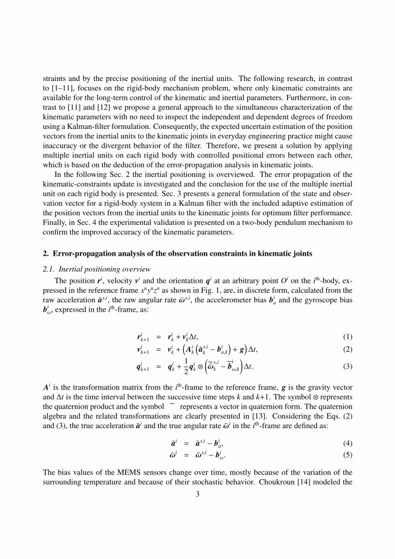
2.1. Inertial positioning overviewThe position ri, velocity vi and the orientation qi at an arbitrary point Oi on the ith-body, ex-

pressed in the reference frame xnynzn as shown in Fig. 1, are, in discrete form, calculated from theraw acceleration as,i, the raw angular rate ωs,i, the accelerometer bias bi

a and the gyroscope biasbiω, expressed in the ith-frame, as:

rik+1 = ri

k + vik∆t, (1)

vik+1 = vi

k +(Ai

k

(as,i

k − bia,k

)+ g

)∆t, (2)

qik+1 = qi

k +12

qik ⊗

(˜ωs,ik − b

iω,k

)∆t. (3)

Ai is the transformation matrix from the ith-frame to the reference frame, g is the gravity vectorand ∆t is the time interval between the successive time steps k and k+1. The symbol ⊗ representsthe quaternion product and the symbol ˜ represents a vector in quaternion form. The quaternionalgebra and the related transformations are clearly presented in [13]. Considering the Eqs. (2)and (3), the true acceleration ai and the true angular rate ωi in the ith-frame are defined as:

ai = as,i − bia, (4)

ωi = ωs,i − biω. (5)

The bias values of the MEMS sensors change over time, mostly because of the variation of thesurrounding temperature and because of their stochastic behavior. Choukroun [14] modeled the

3

bias values as constants; however, the identification of the stochastic parameters in the time domainusing the Allan variance [15, 16] shows that the long-term changing of the bias can be modeled asthe exponentially correlated Gauss-Markov process [17]. This approach of the stochastic modelingat the same time satisfies the condition of the normally distributed noise if the sensor bias isobserved within the state vector in the Kalman filter. Furthermore, because it is hard to distinguishand separate different sources in practice, Gebre [18] showed that the Gauss-Markov model canalso be efficient when the temperature changes slowly in the surrounding environment. Followingthe latter approach, the bias vectors ba and bω can be written in discrete form as [19]:

bia,k+1 = bi

a,k e−βia∆t, (6)

biω,k+1 = bi

ω,k e−βiω∆t, (7)

where the components of the bias vectors βia and βi

ω stand for the inverse values of the correlationtimes τi

c,a and τic,ω of the accelerometer and the gyroscope, respectively.

2.2. Error-propagation analysis in kinematic jointsThe error of the kinematic parameters increases rapidly during the integration procedure over

time if Eqs. (1)-(7) are used in a straightforward manner. If only the kinematic constraints are con-sidered within the Kalman-filter formulation to minimize this error, the rigid-body system shouldfulfill the conditions that each rigid body needs at least one kinematic relation to the other bodiesand at least one rigid body in the system must have a kinematic relation to the environment. Inanother case an additional aiding system should be used. However, the accuracy of the kinematicconstraints, such as the position and velocity conditions in kinematic joints, also has an influenceon the efficiency of the Kalman filter.

Assuming the arbitrary lth-kinematic joint between the ith- and jth-body in Fig. 1, the positionvector rl

c and the velocity vlc at the point Cl can be written with respect to the ith-body:

rlc = ri + Aiui, (8)

vlc = vi + Ai

(ωi × ui

), (9)

where ui represents the position vector from the inertial unit on the ith-body to the kinematic jointCl, expressed in the ith-body frame. Analogously, Eqs. (8) and (9) can be written with the respectto the jth-body. The position vector ui is estimated when the inertial unit is fixed to the body andis assumed to be constant in the following deduction. The opposite case will be discussed laterin the text. The error propagation of the position vector δrl

c and the velocity δvlc can be deduced

with the total differentiation of Eqs. (8) and (9). Additionally, we must consider the followingequality [13]:

A{q + δq} = A(I + δφ×

), (10)

that describes the change of the transformation matrix A because of the orientation change δq.δφ× is a skew-symmetric matrix of the vector φ, which represents the imaginary vector part of thequaternion change δq. It follows that:

δrlc = δri − Ai(ui)×δφi + Aiδui, (11)

δvlc = δvi − Ai

(ωi × ui

)×δφi − Ai(ui)×δωi + Ai(ωi)×δui, (12)4

where × stands for the skew-symmetric matrix of the observed vector. Analyzing Eqs. (11) and (12)the errors δri, δvi, δφi and the angular rate error δωi, which can be simplified to the error ofthe gyroscope bias δbi

ω, represent the group of errors that are related to the estimated position,velocity, quaternion and bias parameter for the ith-body described by Eqs. (1)-(3) and (7). If theseparameters are observed within the state vector in the Kalman filter, using the theory of [19], theirerrors should be normally distributed and their mean values should be equal to zero.

The remaining error δui is the error of the estimated position vector ui. This error mechanismcannot be assumed to be normally distributed, because it is hard to achieve the accuracy of theposition vector ui to the level of the measurement-tool accuracy in everyday practice. Such a casecould be the exact position of the accelerometer, which is hidden inside the inertial unit. Further,the accessibility to the kinematic joints could be reduced and consequently, the position vectorscould only be estimated. Furthermore, the measurement tool could have inadequate accuracy.Therefore, the error vector δui can only have an initial estimation. However, if the error mecha-nism, which has an influence on the observation constraint, is not normally distributed there mightbe inferior performance from the Kalman filter, which can also lead to a divergence.

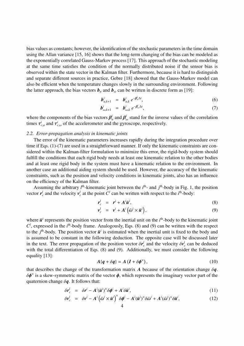
Therefore, an accurate estimation of the position vectors from the inertial units to the kinematicjoints represents an important step toward an accurate estimation of the kinematic parameters. Inthe following step the procedure for minimizing this error will be deduced.Fig. 2 presents the samearbitrary rigid bodies with the kinematic joint as Fig. 1, with the difference being that there is anarbitrary number of inertial units on each body. Consider the position vector ui

mn between themth-unit and nth-unit on the ith-body, expressed in the reference frame:

rin − ri

m = uimn. (13)

In addition, the following relation can be written regarding the equality of the description of theposition vector rl

c = rlc,m = rl

c,n of the kinematic joint Cl with respect to the mth-unit and the nth-uniton the ith-body:

rlc,n − rl

c,m = rin + ul,i

n − rim − ul,i

m = rin + Ai

nul,in − ri

m − Aimul,i

m = 0, (14)

where ul,im and ul,i

n represent the position vectors from the mth-unit and the nth-unit on the ith-bodyto the arbitrary lth-kinematic joint. The ¯ above these vectors indicates that they are expressedin the local sensor frames. Furthermore, considering Eqs. (13) and (14) it is possible to show thefollowing relation:

ul,im − ul,i

n = uimn. (15)

Finally, the error propagation of the position vector δrlc,m and the velocity vector δvl

c,m of the l-kinematic joint with respect to the ith-body can be written with a consideration of Eq. (15):

δrlc,m = δri

m − Aim(ul,i

m)×δφim +

(δul,i

n + δuimn

), (16)

δvlc,m = δvi

m − Aim

(ωi

m × ul,im

)×δφi

m − Aim(ul,i

m)×δωim + (ωi

m)×(δul,i

n + δuimn

), (17)

whereωm represents the angular rate of the mth-unit expressed in the reference frame. Analogously,we can write the error propagation of the position vector δrl

c,n and the velocity vector δvlc,n of the

5

lth-kinematic joint. However, in Eqs. (12) and (13) there is another error mechanism δuimn, which

is related to the error of the position vector between the mth and nth-units. In contrast to the errorsδul,i

m and δul,in , the amplitude of δui

mn can be minimized if the position vector uimn is controlled when

the inertial units are placed on the rigid body. This action is possible in practice with a plannedallocation of inertial units. δui

mn can be minimized to the accuracy level, which is negligiblecompared to the amplitude of the bodies’ movement. If the described assumption is fulfilled,the position vectors from the inertial units to the kinematic constraints can be estimated togetherwith the kinematic and sensor parameters within the state vector in the Kalman filter, becausethe position vectors between the inertial units, such as ui

mn, represent the additional positionalconstraints.

3. Formulation of the kinematic model

3.1. Process modelIn general, the kinematic parameters described with Eqs. (1)-(5) can be observed at every

point on the arbitrary ith-body, where the inertial units are attached. However, while the positionand velocity vectors differ between each other during the motion in these points, the orientationof the ith-body remains the same. Therefore, in order to reduce the number of sensors on everybody, the arbitrary n number of inertial units actually represents the n number of accelerometersand only one gyroscope. If the angular rate is measured at the mth-unit, then the state vector xi ofthe kinematic and sensor parameters on the ith-body can be written as:

xi =((ri

1)T , (vi1)T , (bi

a,1)T , · · · , (rim)T , (vi

m)T , (bia,m)T , · · · , (qi

m)T , (biω,m)T

)T=

=((xi

1)T , · · · , (xim)T , · · · , (qi

m)T , (biω,m)T

)T. (18)

If the system consists of n rigid bodies, then the state vector x of all the observed kinematic andsensors parameters is:

x =((x1)T , · · · , (xi)T , · · · , (xn)T

)T(19)

Considering the assumption of observing the position vectors from the inertial units to the kine-matic joints, a state vector xu can be additionally written:

xu = ((u1,11 )T , · · · , (ul,i

m)T , · · · )T . (20)

These position vectors are modeled as constants; therefore, the arbitrary position vector ul,im from

the mth-inertial unit on the ith-body to the lth-kinematic joint between two successive time steps iscalculated as:

ul,im,k+1 = ul,i

m,k. (21)

Finally, all the observed parameters are joined in the state vector xkin:

xkin =(xT , xT

u

)T. (22)

6

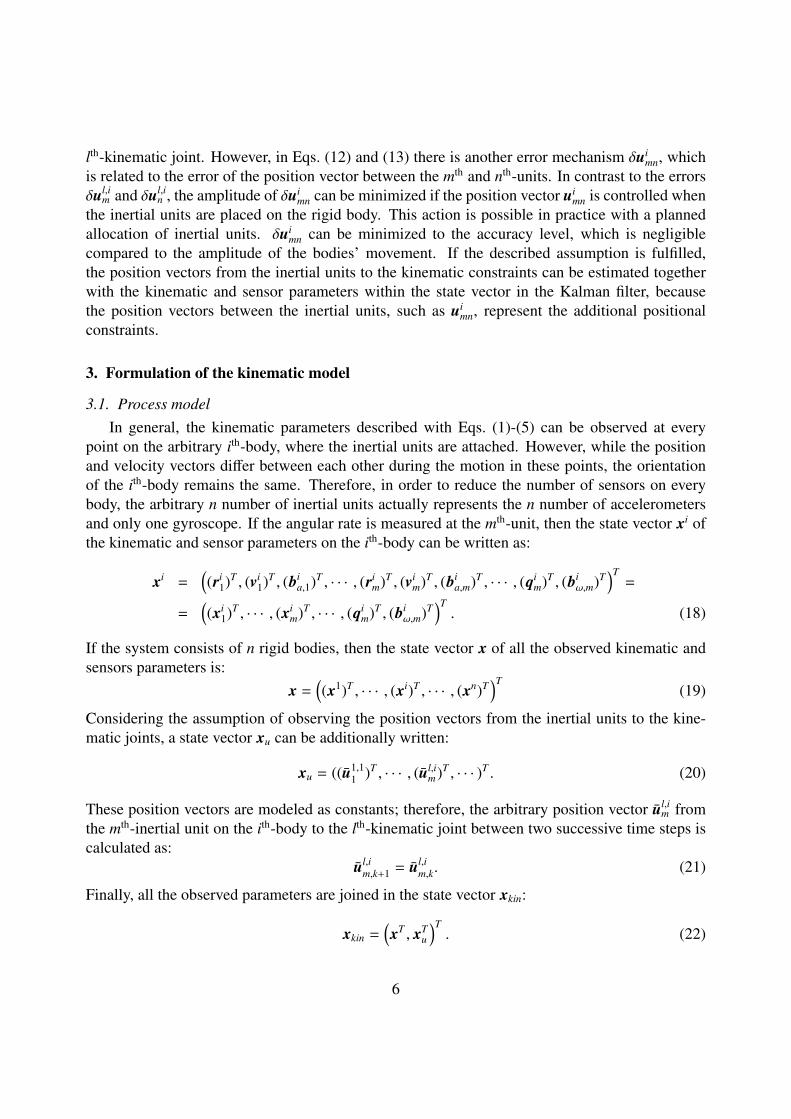
The nonlinear relation between the two successive observation steps of the state vector xkin de-scribes a function f kin:

xkin,k+1 = f kin(xkin,k, as,11,k, ω

s,11,k, . . . , a

s,im,k, ω

s,im,k, . . .) + wk (23)

where wk represents the process noise with the covariance matrix Qkin =

[Q 00 Qu

]= E[wkwT

k ].

Because the parameters of the state vector xkin have nonlinear relations, the extended Kalmanfilter (EKF) is used in this study with the total formulation [20]. Therefore, the state transitionmatrix Φk in k-th step is defined as:

Φk(xkin,k) =∂ f kin(xkin,k)

∂xkin. (24)

The details of the Kalman filter, followed by this research, are discussed elsewhere [14, 18, 19].

3.2. Observation modelObserving the kinematic constraints between the rigid bodies and the position vectors between

the inertial units on every rigid body, three types of observation equation can be defined:

1. Observation of the kinematic constraints: The number of these constraints depends on thenumber and the types of the kinematic joints. In general, the mathematical description ofthese joints, such as spherical, cylindrical, translational joint, etc., are discussed in detailsby Shabana in [21]. Regarding the parameters in the state vector x the positional constraintequations hcr, the velocity constraint equations hcv and the orientational constraint equationshcφ should be defined if they are possible. For the arbitrary lth-kinematic joint the constraintsare joined in the observation vector yl

c:

ylc = hl

c (xkin) =

hl

cr (xkin)hl

cv (xkin)hl

cφ (xkin)

= 0. (25)

For the rigid-body system all the available kinematic constraints are joined in the followingobservation vector:

yc = hc(xkin) =((h1

c)T , · · · , (hlc)

T , · · ·)T

= 0, (26)

2. Observation of the kinematic parameters at different positions on every rigid body: Theseobservations relate to Eq. (13). Because the inertial values are primarily expressed in thelocal coordinate systems of the inertial units, we first write the transformation matrix Amn

that describes the relation between the local coordinate systems of the arbitrary mth- andnth-inertial units:

Ain = Ai

m Aimn, (27)

The transformation matrix Amn is constant if the inertial units are fixed on the rigid body.Assuming the observation in the coordinate system of the mth-inertial unit, the positional and

7

velocity constraints in the vector yiI,mn can be defined between the origin of the mth- and the

nth-inertial units on the ith-body, based on the known position vector uimn, which is written as

uim,mn in the mth-coordinate system:

yiI,mn = hi

I,mn(xim, x

in, u

im,mn) =

(ri

n − rim − Ai

muim,mn

vin − vi

m − Aim(ωi

m × uim,mn)

)= 0. (28)

Observing the whole system the observation vector yI can be written as:

yI = hI(x) = ((y1I,12)T , · · · , (yi

I,mn)T , · · · )T = 0. (29)

3. Observation of the position vectors from the inertial units to the kinematic joints: The thirdgroup of observation equations comes from Eq. (15). Observing the position vectors fromthe arbitrary mth- and nth-inertial units on the ith-body to the lth-kinematic joint, the observa-tion vector yl,i

u,mn is:

yl,iu,mn = hl,i

u,mn(ul,im , u

l,in , u

im,mn) = ul,i

m − Aimnul,i

n − uim,mn = 0. (30)

Regarding all the difference vectors on all the rigid bodies, the observation vector yu isdefined as:

yu = hu(xu) = ((y1,1u,12)T , · · · , (yl,i

u,mn)T , · · · )T = 0. (31)

The second and third groups of the observation equations can be defined because of the use ofthe multiple inertial units on every rigid body and, consequently, they represent the additionalconditions for the correction of the kinematic parameters within the state vector xkin. All threegroups of observations are grouped into the observation vector y:

y = h(xkin) = (yTc , y

TI , y

Tu )T . (32)

The matrix H represents the relation between the predicted state x −kin and the observations atthe linearization point of the function h and is defined as:

H =

Hc

HI

Hu

=

∂hc∂xkin∂hI∂xkin∂hu∂xkin

. (33)

The covariance matrix R of the normally distributed observation deviations is also divided intothree parts:

R =

Rc 0 00 RI 00 0 Ru

. (34)

The covariance matrix Rc in practice depends on the tightness conditions in the joints, whilethe covariance matrices RI and Ru depend on the accuracy of the allocation of the inertial unitsbetween each other on every rigid body. The part of RI that relates to the velocity observations,also depends on the normally distributed angular rate noise. Consequently, the expected deviationin the kinematic joints and the accuracy of the inertial unit positioning also influence the accuracyof the observed state vector xkin.

8

3.3. Adaptive estimation of the joint position vectorsThe initial estimation of the covariance matrix Qu describes the initial, normally distributed

deviations of the position vectors from the inertial units to the kinematic joints. If the positionvectors in xu converge to the exact values, then the values of the covariance matrix Qu shoulddecrease over time. For the optimum operation of the Kalman filter the covariance matrix Qu mustbe adjusted with respect to the estimated deviation of the position vectors in xu.

The deviation of the state vector xu can be estimated in every kth-step of the Kalman filter whenthe predicted vector x −u,k+1 is compared to the observation vector yu,k+1:

∆yu,k+1 = yu,k+1 − Hu,k+1 x −u,k+1, (35)

where ∆yu,k+1 represents the residual error of the position vectors from the inertial units to thekinematic joints. If the state vector xu converges to the true value, the covariance matrix Qumust be adjusted in such a way that the residual error ∆yu,k+1 is minimized. In this study theminimization process follows the approach in [14] and is adapted for the estimation of the statevector xu.

For every pair of position vectors ul,im and ul,i

n on the ith-body the minimization equation J(µi)can be written [14]:

J(µi) = |∆yiu,k+1(∆yi

u,k+1)T − Si−k+1(µi)|2, (36)

where | | stands for the Frobenius norm of the observed matrix. Vector ∆yiu,k+1 consists of all the

residual errors that can be determined on the ith-body using arbitrary yl,iu,mn vectors:

∆yiu,k+1 =

∆yl,i

u,12,k+1...

∆yl,iu,mn,k+1...

. (37)

Si−k+1 represents the part of the Kalman gain factor S−k+1 that relates to the covariance matrix of the

residual error ∆yiu,k+1. S−k+1 follows as [14]:

S−k+1 =(Hk+1 P−k+1HT

k+1 + Rk+1

)−1. (38)

µi is a minimization factor for the adjustment of the covariance matrix Qu at the position of thesubcovariance matrices Qi

u,1, . . . , Qiu,m, . . . on the ith-rigid body. It is deduced in [14] that the factor

µi is defined as:

µi =tr(∆yi

u,k+1(∆yiu,k+1)T − N1)LT

1

tr(L1LT1 )

(39)

and

µi =

{µi; µi > 00; µi ≤ 0 . (40)

9

The components N1 and L1 in Eq. (34) are calculated as follows [14]:

N1 = H?u,k+1IH?T

u,k+1, (41)

L1 = H?u,k+1 P?

k+1H?T

u,k+1 + R?k+1. (42)

The matrices H?u,k+1, P?

k and R?k+1 represent the parts of the matrices Hu,k+1, P−k+1 and Rk+1 in

the Kalman filter that relate to the position vectors from the inertial units to the kinematic jointson the ith-body:

H?u,k+1 =

Hl,i

u,12,k+1...

Hl,iu,mn,k+1...

, (43)

P?k+1 =

P−ul,i

1 ,k+1· · · · · · 0

.... . .

...... P−

ul,im ,k+1

...

0 · · · · · ·. . .

, (44)

R?k+1 =

Rl,i

u,12,k+1 · · · · · · 0...

. . ....

... Rl,iu,mn,k+1

...

0 · · · · · ·. . .

. (45)

When the coefficient µi is determined, the adapted covariance matrices of the position vectors fromthe inertial units to the arbitrary lth-kinematic joint on the arbitrary ith-body are:

Ql,iu,1 = . . . = Ql,i

u,m = . . . = µiI. (46)

3.4. Discussion on the kinematic modelThe presented kinematic model is deduced generally for the multiple inertial units on every

rigid body with controlled position vectors between the inertial units. Fig. 3 summarize the appli-cation of the proposed process and the observation model within the Kalman-filtering iteration.However, the use of the multiple inertial units on every rigid body would result in unnecessarycosts and processing power, especially if large systems would be observed. Therefore, the pre-sented approach would follow the simplification of the use of only two inertial units on every rigidbody, because in this case the condition of the controlled position vectors is also satisfied. Theselection of the same number of accelerometers was also made in practice by Cheng [12], wherehe showed an improved performance of the angle determination at lower rotation speeds.

In Sec. 2.2 we consider the constant position vectors from the inertial units to the kinematicjoints. However, the presented approach should not differ if these position vectors are time depen-dent, because we showed in Sec. 3.1 that they are included in the state vector xkin. On the otherhand, the advantage of the constant position vectors from the inertial units to the kinematic jointsis the possibility of their elimination from state vector xkin, when they converge to the real values.

10

4. Experimental validation

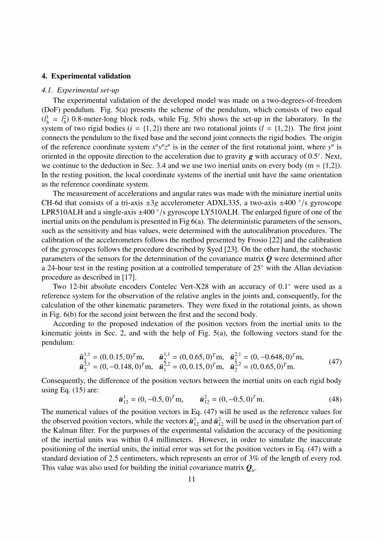
4.1. Experimental set-upThe experimental validation of the developed model was made on a two-degrees-of-freedom

(DoF) pendulum. Fig. 5(a) presents the scheme of the pendulum, which consists of two equal(l1

b = l2b) 0.8-meter-long block rods, while Fig. 5(b) shows the set-up in the laboratory. In the

system of two rigid bodies (i = {1, 2}) there are two rotational joints (l = {1, 2}). The first jointconnects the pendulum to the fixed base and the second joint connects the rigid bodies. The originof the reference coordinate system xnynzn is in the center of the first rotational joint, where yn isoriented in the opposite direction to the acceleration due to gravity g with accuracy of 0.5◦. Next,we continue to the deduction in Sec. 3.4 and we use two inertial units on every body (m = {1,2}).In the resting position, the local coordinate systems of the inertial unit have the same orientationas the reference coordinate system.

The measurement of accelerations and angular rates was made with the miniature inertial unitsCH-6d that consists of a tri-axis ±3g accelerometer ADXL335, a two-axis ±400 ◦/s gyroscopeLPR510ALH and a single-axis ±400 ◦/s gyroscope LY510ALH. The enlarged figure of one of theinertial units on the pendulum is presented in Fig 6(a). The deterministic parameters of the sensors,such as the sensitivity and bias values, were determined with the autocalibration procedures. Thecalibration of the accelerometers follows the method presented by Frosio [22] and the calibrationof the gyroscopes follows the procedure described by Syed [23]. On the other hand, the stochasticparameters of the sensors for the determination of the covariance matrix Q were determined aftera 24-hour test in the resting position at a controlled temperature of 25◦ with the Allan deviationprocedure as described in [17].

Two 12-bit absolute encoders Contelec Vert-X28 with an accuracy of 0.1◦ were used as areference system for the observation of the relative angles in the joints and, consequently, for thecalculation of the other kinematic parameters. They were fixed in the rotational joints, as shownin Fig. 6(b) for the second joint between the first and the second body.

According to the proposed indexation of the position vectors from the inertial units to thekinematic joints in Sec. 2, and with the help of Fig. 5(a), the following vectors stand for thependulum:

u1,11 = (0, 0.15, 0)T m, u1,1

2 = (0, 0.65, 0)T m, u2,11 = (0,−0.648, 0)T m,

u2,12 = (0,−0.148, 0)T m, u2,2

1 = (0, 0.15, 0)T m, u2,22 = (0, 0.65, 0)T m.

(47)

Consequently, the difference of the position vectors between the inertial units on each rigid bodyusing Eq. (15) are:

u112 = (0,−0.5, 0)T m, u2

12 = (0,−0.5, 0)T m. (48)

The numerical values of the position vectors in Eq. (47) will be used as the reference values forthe observed position vectors, while the vectors u1

12 and u212 will be used in the observation part of

the Kalman filter. For the purposes of the experimental validation the accuracy of the positioningof the inertial units was within 0.4 millimeters. However, in order to simulate the inaccuratepositioning of the inertial units, the initial error was set for the position vectors in Eq. (47) with astandard deviation of 2.5 centimeters, which represents an error of 3% of the length of every rod.This value was also used for building the initial covariance matrix Qu.

11

According to Eq. (27) the initial difference in the orientation of the inertial units must be de-termined despite the fact that the positioning of the inertial units on each rigid body is controlled.Using the comparison of the response of the calibrated accelerometers in different static posi-tions, the matrices A1

12 and A212 can be defined using the least-squares method. For the case of

the proposed experiment these matrices are functions of the following Euler angles with the zyxsuccessive rotations [21]:

Θ112 = (0.36◦,−0.4◦, 0.81◦)T , Θ2

12 = (0.54◦, 0.02◦,−0.45◦)T . (49)

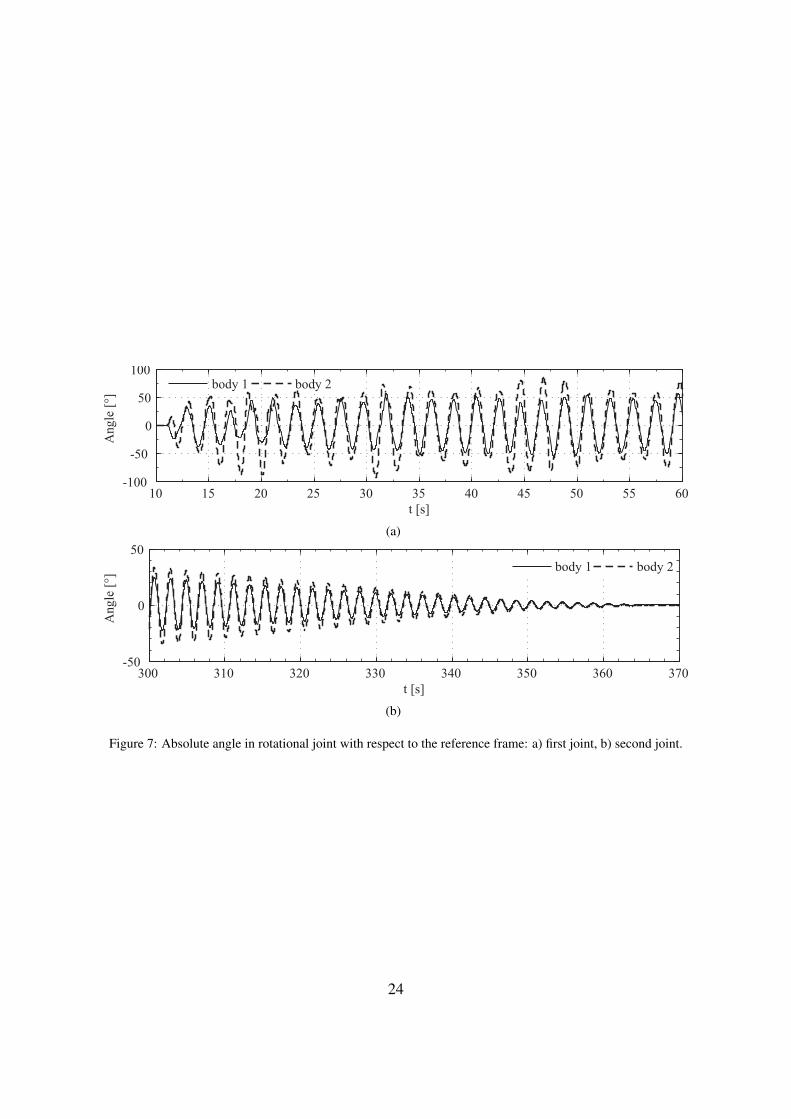
For the experimental validation we proposed a combination of the different motion regimes.From the initial resting position, the pendulum was forced into accelerated motion. During themotion the pendulum was exposed to accelerations and decelerations until it swung back to theinitial position. The motion was observed for approximately six minutes. For reasons of clarity,Fig. 7(a) presents the change of the absolute angle in the rotational joint with respect to the refer-ence frame in the first minute of motion, while Fig. 7(b) presents the change of the absolute anglein the last minute, when the pendulum swung down.

4.2. Kinematic model of a 2-DoF pendulumFor the observed 2-DoF pendulum, according to Eq. (18) the state vectors x1 and x2 that

describe the kinematic and sensor parameters for the first and second rigid bodies can be definedas:

x1 =((r1

1)T , (v11)T , (b1

a,1)T , (r12)T , (v1

2)T , (b1b,2)T , (q1

t )T , (b1ω)T

)T, (50)

x2 =((r2

1)T , (v21)T , (b2

a,1)T , (r22)T , (v2

2)T , (b2b,2)T , (q2

t )T , (b2ω)T

)T, (51)

As shown in Fig. 5(a), the state vector xu of the position vectors to the kinematic constraintsfor the observed pendulum can be written considering Eq. (20):

xu =

((u1,1

1

)T,(u1,1

2

)T,(u2,1

1

)T,(u2,1

2

)T,(u2,2

1

)T,(u2,2

2

)T)T. (52)

Using Eqs. (22) the state vector xkin of the kinematic model is therefore:

xkin =((x1)T , (x2)T , xT

u

)T. (53)

Furthermore, the observation vector y in Eq. (32) follows to the separation on three parts. Thevector of kinematic constraints yc in the kinematic joints regarding Eq. (26) is defined as:

yc =(

(h1cr)

T , (h1cv)T , (h1

cφ,1)T , (h1cφ,2)T , (h2

cr)T , (h2

cv)T , (h2cφ,1)T , (h2

cφ,2)T)T

=

=

r11 + r1

2 + A1(u1,1

1 + A112u1,1

2

)v1

1 + v12 + A1

(ω1×

(u1,1

1 + A112u1,1

2

))(en

z )T(A1e1

x1

)(en

z )T(A1e1

y1

)r1

1 + r12 + A1

(u2,1

1 + A112u2,1

2

)− r2

1 − r22 − A2

(u2,2

1 + A212u2,2

2

)v1

1 + v12 + A1

(ω1×

(u2,1

1 + A112u2,1

2

))− v2

1 − v22 − A2

(ω2×

(u2,2

1 + A212u2,2

2

))(en

z )T(A2e2

x1

)(en

z )T(A2e2

y1

)

= 0, (54)

12

where h1cr represents the positional constraints in the rotational joint between the base and the first

rod. Two independent constraints with respect to the first and second inertial frames on the firstbody:

r11 + A1u1,1

1 = 0, r12 + A1 A1

12u1,12 = 0 (55)

are simplified in one equation to minimize the total number of equations. Similarly, the functionhcv represents the velocity constraints in the first joint, while h2

cr and h2cv stand for the positional

and velocity constraints in the second joint. The functions h1cφ,1, h1

cφ,2, h2cφ,1 and h2

cφ,2 stand for theconstraints that are related only to the rotational joint. The rotation is available only around thezn-axis in the reference frame. These constraints are not dependent on the positional and velocityconstraints; therefore, they are written with the unity vectors en

z , e1x1

, e1y1

, e2x1

and e2y1

, which areexpressed in the appropriate coordinate frames.

The observation vector yI with respect to Eq. (29) is defined as:

yI =

(h1

I,12(x1, u11,12)

h2I,12(x2, u2

1,12)

)=

r1

2 − r11 − A1u1

1,12v1

2 − v11 − A1((ω1)×u1

1,12)r2

2 − r21 − A2u2

1,12v2

2 − v21 − A2((ω2)×u2

1,12)

= 0, (56)

and finally, the observation vector yu with respect to Eq. (31) follows as:

yu =

h1,1

u,12(u1,11 , u1,1

2 , u11,12)

h2,1u,12(u2,1

1 , u2,12 , u1

1,12)h2,2

u,12(u2,21 , u2,2

2 , u21,12)

=

u1,1

1 − A112u1,1

2 − u11,12

u2,11 − A1

12u2,12 − u1

1,12u2,2

1 − A212u2,2

2 − u21,12

= 0. (57)

The covariance matrix R using Eqs. (34) was defined according to the expected deviations in thekinematic constraints. The covariance matrix Rc depends on the tightness in the joint bearings.Because of the tight connection the positional deviation was set to 0.1 millimeter. Furthermore,the positional deviations in the covariance matrices RI and Ru depend on the accuracy of themeasurement tool or on the accuracy of the positioning procedure between inertial units. In thisstudy, the deviation was found to be 0.4 millimeter. On the other hand, the deviations of thevelocity constraints depend mainly on the normally distributed noise in the angular rate data. Theorientational constraints were limited to a 0.1◦ deviation.

4.3. Analysis of the experimental resultsIn the experimental analysis the presented adaptive Kalman formulation with the estimation

of the position vectors from the inertial units to the kinematic joints (KF1) will be compared withthe formulation that does not consider the estimation of the position vectors from the inertial unitsto the kinematic joints in the state vector xkin (KF2). However, the results calculated straightfor-wardly from the inertial data will not be presented because the errors increase enormously in a fewseconds.

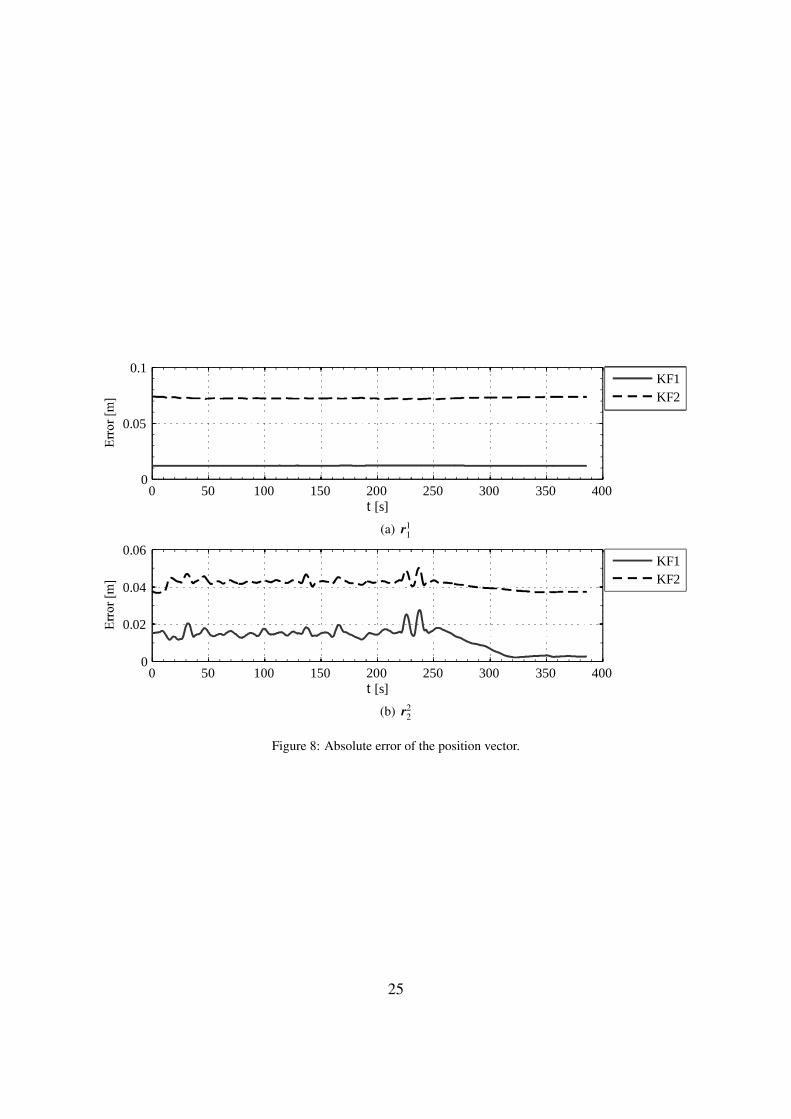
In the first step the errors of the kinematic parameters are examined. Fig. 8 presents the abso-lute error value of the position vector r1

1 on the first body and of the position vector r22 on the second

body, expressed in the reference frame. The results show the minimized and steady errors of the

13

position vectors when the KF1 formulation with the adaptive estimation is used. In contrast, theKF2 formulation also shows steady, but higher, absolute errors. These errors are the consequenceof the inaccurate initial estimation of the position vectors from the inertial units to the kinematicjoints and, furthermore, they influence the assumption of the Kalman filter that the error of theobservation vector yc is normally distributed with the zero mean value. A larger deviation of theposition vector r2

2 is related to the fact that this inertial unit has the greatest distance from the baseof the pendulum. Therefore, when the pendulum is accelerated or decelerated, a possible move-ment in the zn-axis can reduce the performance of the filter. When the pendulum swung down theerror also decreases. Regarding the size of the pendulum in Fig. 5 and the large angle changesover time in Fig. 7, the constant error under 2% shows the appropriate approach when using theadaptive formulation.

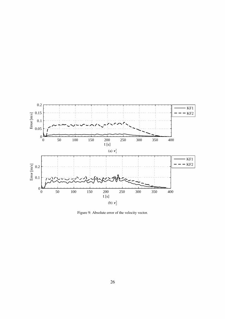
Fig. 9 shows the absolute error of the velocity vectors v11 on the first body and v2

2 on the secondbody in the reference frame. The KF1 formulation shows better or equivalent results compared tothe KF2 formulation. However, there is a clear difference in the error values when the pendulum isin the resting position or when it moves between 10 and 250 seconds. The difference can be relatedto the noise in the angular rate data, which affects the observations in Eqs. (54) and (56). How-ever, the absolute errors are consistently under 2%, which again supports the use of the proposedadaptive filter.

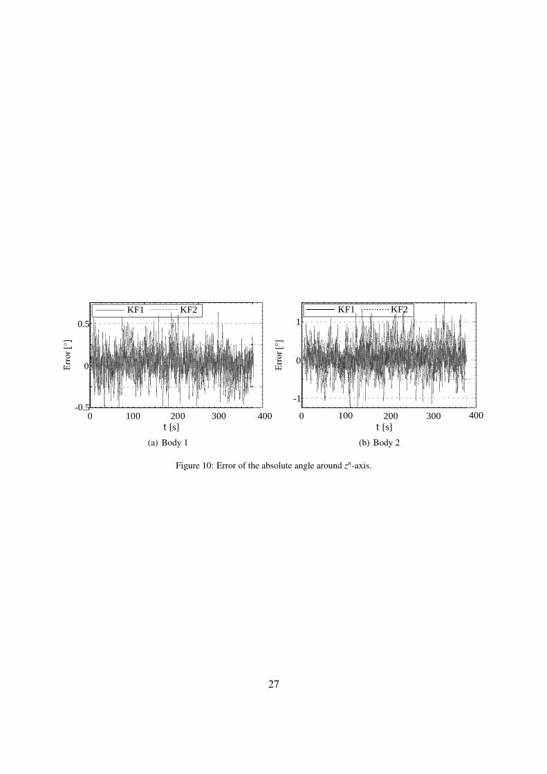
Another kinematic parameter is the orientations of the rigid bodies. Fig. 10 presents the ab-solute angle error around the zn-axis in the reference frame. The angle is calculated from theestimated quaternion [13]. KF1 again shows a better angle estimation over the KF2 formulations.The errors of the KF1 and KF2 approaches have constant zero mean values over time. Betterresults of the KF2 formulation, which shows inferior positional and velocity results, are the conse-quence of good orientation constraints in the rotational joint and because the position vectors fromthe inertial units to the kinematic joint do not directly affect the orientation constraints in Eq. (54).

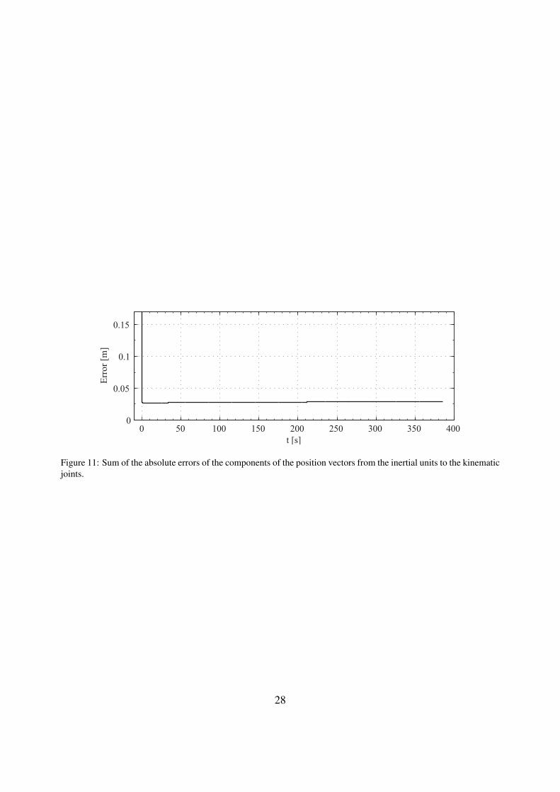
In the second step the estimation of the position vectors from the inertial units to the kinematicjoints is discussed. Fig. 11 shows the absolute sum of all the position-vector errors. When using theadaptive approach the initial error value of 0.1704 meter decreases to a value of 0.0274 meter overapproximately 100 iterations and stays constant or changes negligibly over the entire observationtime. Considering the estimated and the reference position vectors in Eq. (47) the error vectorscan be calculated:

∆u1,11 = (0,−0.0002, 0.013)T m, ∆u1,1

2 = (0,−0.0004, 0.013)T m,∆u2,1

1 = (0, 0.0018,−0.0123)T m, ∆u2,12 = (0, 0.0018,−0.0123)T m,

∆u2,21 = (−0.0017,−0.0011, 0.01)T m, ∆u2,2

2 = (−0.0017,−0.0011, 0.01)T m.(58)

The deviations in the x and y-axis in the local frames show a negligible error, while the errorsin the z-axis in the local frames deviate constantly by around 1 centimeter. These deviations canbe related to the positioning and orientation of the inertial units on the rigid bodies with respectto the reference frame, because the motion is tightly restricted in the z-axis of the reference andlocal frames, but in practice there could be minor deviations. However, the rapid convergenceof the position vectors from the inertial units to the kinematic joints is the consequence of thethe adaptive approach, which adjust the initial covariance matrix Qu toward the zero values withrespect to the residual error of the observed position vectors.

14

The use of the adaptive approach with multiple inertial units on every rigid body might causea problem with the observation of the state vector xkin in real time if there are many bodies inthe system or if there are many constraint equations. For these reasons the approach with themultiple inertial units can only provide the calibration procedure for the estimation of the positionvectors. On the other hand, when the position vectors from the inertial units to the kinematic jointsconverge, the redundant kinematic parameters in the state vector xkin and in the observation vectory can be eliminated in a way that we observe the kinematic parameters with only one inertial uniton every rigid body.

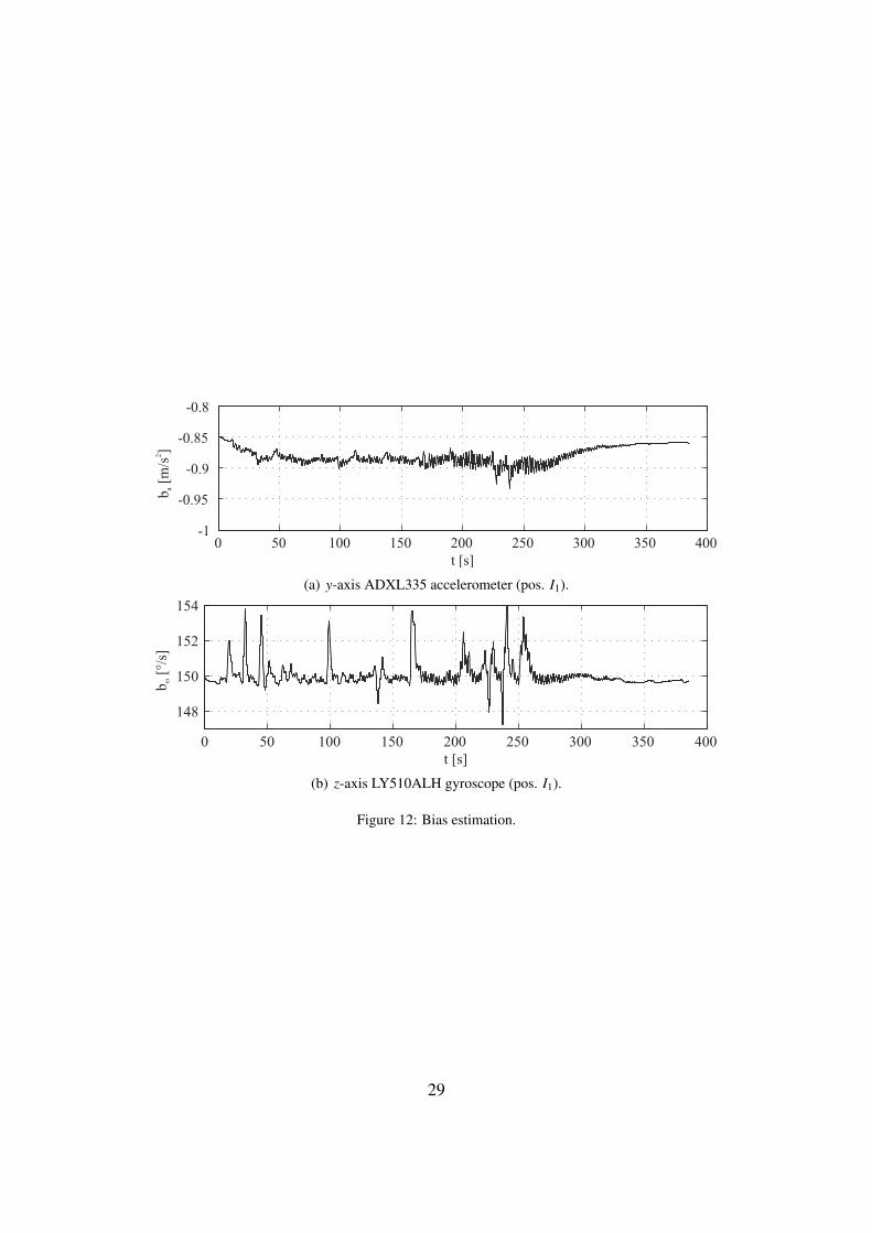
In the last step the estimation of the sensors’ bias vectors is discussed. Fig. 12 shows theestimation of the bias values on the selected axes of the accelerometer and the gyroscope. Despitethe assumptions of the exponentially correlated change of the bias values, the figures show thatthe bias can also change because of the other influences, such as the change of the temperatureor the internal changes in the sensors, which do not have the exponentially correlated stochasticbehavior. The Kalman filter considers the estimation of the bias values with respect to the processand observation formulation.

5. Conclusion

In this study we present an approach to minimize the error of the kinematic parameters of arigid body system due to the inaccurate positioning of the inertial units on the rigid body for thecase when only the kinematic constraints are used for the correction of the inertial principle withinthe Kalman formulation. Based on the error propagation of the observation equations a generalapproach to the use of multiple inertial units on every rigid body is deduced if we are able tocontrol the position vectors between the inertial units. The method was experimentally validatedon a simple pendulum mechanism with the use of the minimum number of inertial units. Weconfirmed that the adaptive formulation gave better results than the standard formulation withoutan estimation of the position vectors from the inertial units to the kinematic joints.

The proposed approach has an advantage when we do not know the dynamics of the observedmechanism in advanced, because the independent and dependent parameters are observed simulta-neously in the state vector. Therefore, this approach offers a quick solution in applications. On theother hand, we must be aware that increasing the number of rigid bodies in the system or possiblya larger number of inertial units can cause problems with the processing power. From the latterpoint of view this approach can represent a calibration procedure for the estimation of the positionvector from the inertial units to the kinematic joints before the kinematic parameters are eventuallyobserved.

The accuracy of the kinematic parameters when only the kinematic constraints are observeddepends not only on the accurate positioning of the inertial units, but in general on the level ofaccuracy in the observation equations. A high level of noisy observation or a deviation from theassumed normally distributed noise can result in poorer performance or divergence of the Kalmanfilter. However, industrial mechanisms usually have well-defined constraints, and therefore thepresented approach offers an appropriate alternative.

15

References

[1] E. D. Roetenberg, P. J. Slycke, P. H. Veltink, Ambulatory position and orientation tracking fusing magnetic andinertial sensing, IEEE Trans. on Bio. Eng. 54 (2007) 883–890.

[2] E. D. Roetenberg, C. T. M. Baten, P. H. Veltink, Estimating body segment orientation by applying inertial andmagnetic sensing near ferromagnetic materials, IEEE Trans. Neural. Sys. & Rehab. Eng. 54 (2007) 883–890.

[3] H. M. Schepers, E. D. Roetenberg, P. H. Veltink, Ambulatory human motion tracking by fusion of inertial andmagnetic sensing with adaptive actuation, Med. Bio. Eng. Comput. 48 (2010) 27–37.

[4] H. M. Schepers, P. H. Veltink, Stochastic magnetic measurement model for relative position and orientationestimation, Meas. Sci. Technol. 21 (2010).

[5] M. Brodie, A. Walmsley, W. Page, Fusion motion capture: a prototype system using inertial measurement unitsand GPS for the biomechanical analysis of ski racing, Sports Technology 1 (2008) 17–28.

[6] M. Supej, 3d measurements of alpine skiing with an inertial sensor motion capture suit and GNSS RTK system,Journal of Sports Sciences 28 (2010) 759–769.

[7] I. Skog, P. Handel, In-car positioning and navigation technologies–a survey, IEEE Transactions on IntelligentTransportation Systems 10 (2009) 4–21.

[8] J. D. Hol, T. B. Scon, H. J. Luinge, P. J. Slycke, F. Gustafsson, Robust real-time tracking by fusing measurementfrom inertial and vision sensors, Journal of Real-Time Image Processing 116 (2007) 266–271.

[9] J. D. Hol, T. B. Schon, F. Gustafsson, Modeling and calibration of inertial and vision sensors, InternationalJournal of Robotics Research 29 (2010) 231–244.

[10] J. Youssef, B. Denis, C. Godin, S. Lesecq, Loosly-coupled IR-UWB handset and ankle-mounted inertial unitfor indoor navigation, International Journal of Robotics Research 29 (2010) 231–244.

[11] J. F. Wagner, Adapting the principle of integrated navigation systems to measuring the motion of rigid multibodysystems, Multibody System Dynamics 1 (2004) 87–110.

[12] P. Cheng, B. Oelmann, Joint-angle measurement using accelerometers and gyroscopes – a survey, IEEE Trans-actions on Instrumentation and Measurement 59 (2010) 404–414.

[13] J. Kuipers, Quaternions and Rotation Sequences, Princeton University Press, 1999.[14] D. Choukroun, I. Y. Bar-Itzhack, Y. Oshman, Novel quaternion kalman filter, IEEE Transactions on Aerospace

and Electronic Systems 42 (2006) 174–190.[15] D. W. Allan, Statistics of atomic frequency standards, Proceedings of the IEEE 54 (1966) 221–230.[16] D. W. Allan, Should the classical variance be used as a basic measure in standards metrology?, IEEE Transac-

tions on Instrumentation and Measurement IM-36 (1987) 646–654.[17] IEEE Aerospace, E. S. Society, IEEE standard specification format guide and test procedure for single-axis laser

gyros, IEEE Std 647–2006, 2006.[18] D. Gebre–Egziabher, R. C. Hayward, J. D. Powell, Design of multi-sensor attitude determination systems, IEEE

Transactions on Aerospace and Electronic Systems 40 (2004) 627–649.[19] R. G. Brown, P. Y. C. Hwang, Introduction to Random Signals and Applied Kalman Filtering, John Wiley &

Sons, Inc., 1997.[20] D.–J. Jwo, T.–S. Cho, Critical remarks on the linearised and extended kalman filters with geodetic navigation

examples, Measurements 43 (2010) 1077–1089.[21] A. A. Shabana, Computational dynamics, A John Wiley & Sons, Inc., 1994.[22] I. Frosio, F. Pedersini, N. A. Borghese, Autocalibration of MEMS accelerometers, IEEE Transactions on

Instrumentation and Measurements 58 (2009) 2034–2041.[23] Z. F. Syed, P. Aggarwal, C. Goodall, X. Niu, N. El–Sheimy, A new multi-position calibration method for MEMS

inertial navigation system, Measurement Science and Technology 18 (2007) 1897–1907.

16

List of Figures

1 Observation of the arbitrary kinematic constraint with one inertial unit on eachrigid body. . . . . . . . . . . . . . . . . . . . . . . . . . . . . . . . . . . . . . . 18

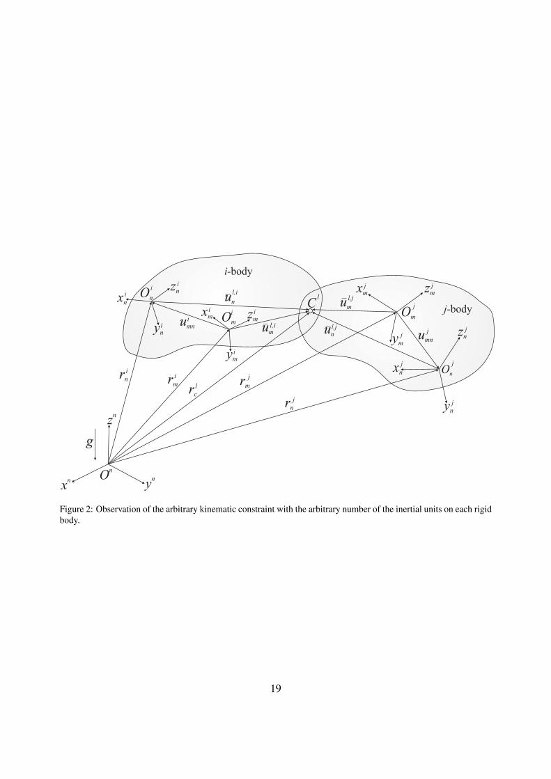
2 Observation of the arbitrary kinematic constraint with the arbitrary number of theinertial units on each rigid body. . . . . . . . . . . . . . . . . . . . . . . . . . . 19

3 Application of the proposed process and observation models within the Kalman-filtering formulation. . . . . . . . . . . . . . . . . . . . . . . . . . . . . . . . . 20

4 2-DoF pendulum. . . . . . . . . . . . . . . . . . . . . . . . . . . . . . . . . . . 215 2-DoF pendulum. . . . . . . . . . . . . . . . . . . . . . . . . . . . . . . . . . . 226 Inertial unit CH-6d and encoder positioning in the rotational joint. . . . . . . . . 237 Absolute angle in rotational joint with respect to the reference frame: a) first joint,

b) second joint. . . . . . . . . . . . . . . . . . . . . . . . . . . . . . . . . . . . 248 Absolute error of the position vector. . . . . . . . . . . . . . . . . . . . . . . . . 259 Absolute error of the velocity vector. . . . . . . . . . . . . . . . . . . . . . . . . 2610 Error of the absolute angle around zn-axis. . . . . . . . . . . . . . . . . . . . . . 2711 Sum of the absolute errors of the components of the position vectors from the

inertial units to the kinematic joints. . . . . . . . . . . . . . . . . . . . . . . . . 2812 Bias estimation. . . . . . . . . . . . . . . . . . . . . . . . . . . . . . . . . . . . 29

17

xn

yn

zn

g

Clx

y

z zj

y j

xj

rcr

uujO

Oj

On

i i

i

i

l

i

r i

r j

i-body

j-body

Figure 1: Observation of the arbitrary kinematic constraint with one inertial unit on each rigid body.

18

nx

ny

nz

g

Cl

xm

ym

zm

zmj

ymj

xmj

rc

um

l,j

OmOm

j

nO

Onxn

On

jxnj

ynj

znjyn

zn

umn unl,j

i

i

i

i i

i

ii

l

umnj

un

l,i

uml,i

i

i-body

j-body

rmirn

i

rmj

rnj

Figure 2: Observation of the arbitrary kinematic constraint with the arbitrary number of the inertial units on each rigidbody.

19

ams,i

ms,i

Q

iadaptive factor

xkin-^

Adaptive extended Kalman filter

xkin,0

R

xkin^

f (x , ..., a , , ...) kin kin m,k m,k

Process model:

Th( x ) =(y y y ) kin c , I , u -^ TTT

Observation model:(x )kin

H( x )kin-^

++

xkin

QuQkin

s,i s,i

Figure 3: Application of the proposed process and observation models within the Kalman-filtering formulation.

20

nx

ny

1x1

1y1

1x2

1y2

2x1

2y1

2x2

2y2

1l

2l

g

u121

u122

u 2,2

2

u 1,1

1

u1,1

2

u2,1

1

u 2,2

2

u2,2

1

1O1

1O2

2O1

2O2

(a) Pendulum scheme. (b) Pendulum set-up in the lab-oratory.

Figure 4: 2-DoF pendulum.

21

nx

ny

1x1

1y1

1x2

1y2

2x1

2y1

2x2

2y2

1l

2l

g

u121

u122

u 2,2

2

u 1,1

1

u1,1

2

u2,1

1

u 2,2

2

u2,2

1

1O1

1O2

2O1

2O2

(a) Pendulum scheme. (b) Pendulum set-up in the lab-oratory.

Figure 5: 2-DoF pendulum.

22

(a) Inertial unit CH-6d. (b) Encoder fixing in the rotationaljoint between two rigid bodies.

Figure 6: Inertial unit CH-6d and encoder positioning in the rotational joint.

23

10 15 20 25 30 35 40 45 50 55 60-100

-50

0

50

100

t [s]

An

gle

[°]

body 1 body 2

(a)

300 310 320 330 340 350 360 370-50

0

50

t [s]

An

gle

[°]

body 1 body 2

(b)

Figure 7: Absolute angle in rotational joint with respect to the reference frame: a) first joint, b) second joint.

24

0 50 100 150 200 250 300 350 4000

0.05

0.1

t [s]

KF1KF2

(a) r11

0 50 100 150 200 250 300 350 4000

0.02

0.04

0.06

t [s]

KF1KF2

(b) r22

Figure 8: Absolute error of the position vector.

25

0 50 100 150 200 250 300 350 4000

0.05

0.1

0.15

0.2

t [s]

KF1KF2

(a) v11

0 50 100 150 200 250 300 350 4000

0.1

0.2

t [s]

KF1KF2

(b) v22

Figure 9: Absolute error of the velocity vector.

26

0 100 200 300-0.5

0

0.5

t [s]400

KF1 KF2

(a) Body 1

0 100 200 300

-1

0

1

t [s]

KF1 KF2

400

(b) Body 2

Figure 10: Error of the absolute angle around zn-axis.

27

0 50 100 150 200 250 300 350 4000

0.05

0.1

0.15

t [s]

Err

or

[m]

Figure 11: Sum of the absolute errors of the components of the position vectors from the inertial units to the kinematicjoints.

28

0 50 100 150 200 250 300 350 400-1

-0.95

-0.9

-0.85

-0.8

t [s]

b[m

/s]

a

2

(a) y-axis ADXL335 accelerometer (pos. I1).

0 50 100 150 200 250 300 350 400

148

150

152

154

t [s]

b[°

/s]

�

(b) z-axis LY510ALH gyroscope (pos. I1).

Figure 12: Bias estimation.

29