b i o s y s t e m s e n g i n e e r i n g 1 0 1 ( 2 0 0 8 ) 1 – 1 2

Avai lab le a t www.sc iencedi rec t .com

journa l homepage : www.e lsev ie r . com/ loca te / i ssn /15375110

Research Paper: AEdAutomation and Emerging Technologies

Minimising the non-working distance travelledby machines operating in a headland field pattern

D.D. Bochtis*, S.G. Vougioukas

Aristotle University of Thessaloniki, Faculty of Agriculture, Department of Agricultural Engineering,

Box 275, 54124 Thessaloniki, Greece

a r t i c l e i n f o

Article history:

Received 29 November 2007

Received in revised form 6 June 2008

Accepted 18 June 2008

Published online 6 August 2008

* Corresponding author.E-mail address: dionmpo@agro.auth.gr (D

1537-5110/$ – see front matter ª 2008 IAgrEdoi:10.1016/j.biosystemseng.2008.06.008

When treating an area of field using agricultural equipment, the field is usually traversed

by a series of parallel tracks using a pattern established by the experience of the operator.

At the end of each track the process is constrained by the ability of the operator to distin-

guish the next track to be followed. The introduction of commercially available auto-

steering or navigation-aid systems for agricultural machines has made it possible to upload

arbitrary field pattern sequences into programmable navigational computers and for the

machines to follow them with precision. This new technology also offers a new perspective

for improving machine field efficiency, since not all field traversal sequences are similar in

terms of total non-working distance travelled.

This paper presents an algorithmic approach towards computing traversal sequences for

parallel field tracks, which improve the field efficiency of machines by minimising the total

non-working distance travelled. Field coverage is expressed as the traversal of a weighted

graph and the problem of finding an optimum traversing sequence is shown to be equiva-

lent to finding the shortest route in the graph. The optimisation is formulated and solved as

a binary integer programming problem. Experimental results show that by using optimum

sequences, the total non-working distance can, depending on operation, be reduced by up

to 50%.

ª 2008 IAgrE. Published by Elsevier Ltd. All rights reserved.

1. Introduction in the field due to non-working travel (Hunt, 2001). A large por-

Modern agricultural machines are, in theory, capable of

achieving very high performance in terms of work rate and

quality. A measure of machine performance during field oper-

ations is its field efficiency, Ef, which is defined (ASAE, 2005) as

the ratio between the productivity of the machine under field

conditions and the theoretical maximum productivity. Field

efficiency is not a constant for a particular machine, but varies

with the size and shape of the field, pattern of field operation,

crop yield, crop moisture, and other conditions. In particular,

the pattern of field operation affects very much the time lost

.D. Bochtis).. Published by Elsevier Ltd

tion of the non-working time occurs during turning and the

strong negative influence of turning time on field efficiency

has been verified experimentally in grain harvesting opera-

tions (Taylor et al., 2002; Hansen et al., 2003), as well as by using

simulation tools (Benson et al., 2002).

When turning on the headland non-working time depends

on the distance travelled during turning (i.e., the length of the

manoeuvre), and the mean turning speed. Some types of ma-

noeuvre are easily executed and consequently can be executed

at high speed, while other types demand skilful driving, or

even reversing, resulting in lower mean speeds and requiring

. All rights reserved.

Nomenclature

A set of arcs of the headland traversal graph G:

A¼ T� T

bl(i) symbolises the type of the traditional where i is the

number of tracks which constitute one block (see

Fig. 6)

cij cost that is associated to each arc Aij of the graph

G. This cost corresponds to the distance that

a machine has to travel in order to go from the end

of track i to the beginning of track j, i.e.,

cij ¼ Lminðji� jjÞ ¼ LminðdijÞDab Euclidean distance between the beginning of the

first track of field a, and the beginning of the first

track of field b

d degree of a manoeuvre which is given by

dij ¼ ji� jj, where i is the track through which the

machine exits at the beginning of the manoeuvre

and j is the track the machine enters at the end of

the manoeuvre

Ef field efficiency

G field headland traversal graph: G ¼ fT;Ag, where T

is the set of graph nodes (which is also the set of

tracks) and A¼ T� T is the set of arcs

G0 the extended graph G0 which contains the field

coverage graph G, plus the node 0 which represent

the machine’s initial position and the node kTk þ 1

which represents the final position of the machine

Jturn(s) the total travelled distance during the turnings at

the headlands for the field track coverage

sequence s (see Eq. (3))

Lmin(d ) the function that gives minimum length of

a manoeuvre of degree d (see Eq. (2))

l the headland length

N set of the nodes of the graph G0: N ¼ TWf0; kTk þ 1g

pð$Þ : T/T bijective function which for every field track,

i˛T, returns the order in which the machine covers

the ith field track

rmin minimum turning radius of the machine

T set of the field track indices. The cardinality kTk of

the set T which is equal to the total number of

tracks that cover the entire field area

w machine effective operating width

xij decision variable of the optimisation problem

which is xij¼ 1 if and only if immediately after

visiting node i the machine travels to node j;

otherwise xij¼ 0

D set Di represents the same tracks as Ti with an offset in

their indexing

3ij stochastic variable that gives the deviation of the

measured manoeuvre distance from the

theoretical minimum manoeuvre distance

P-turn manoeuvre type executed by an agricultural

machine operating in a headland pattern (see

Fig. 2b). The function P(d ) gives the minimum

lengths for a P-turn manoeuvre of degree d (see

Eq. (1))

T-turn manoeuvre type executed by an agricultural

machine operating in a headland pattern (see

Fig. 2c)

s permutation that gives the traversal sequence of

the tracks for the entire field covering. The

notation s* represents the optimal sequence of the

tracks (see Eq. (5)), while the symbol stype the

sequence of the tracks according to the traditional

pattern: type

U-turn manoeuvre type executed by an agricultural machine

operating in a headland pattern (see Fig. 2a). The

function U(d ) gives the minimum lengths for a U-

turn manoeuvre of degree d (see Eq. (1))

b i o s y s t e m s e n g i n e e r i n g 1 0 1 ( 2 0 0 8 ) 1 – 1 22

larger headland areas. Furthermore, some manoeuvres unfav-

ourably influence soil condition (Keller, 2005; Ansorge & God-

win, 2007). Vertical disturbance of the soil is caused by the

weight of the machine, and horizontal disturbances are caused

by changes in the direction of travel. As a consequence the

headland areas constitute ‘‘low productivity’’ field areas (Wit-

ney, 1996). The controlled traffic systems can reduce the im-

pact of the machine but only in the body of the field and not

at the headlands (Bailey, 1997). Finally, the headland manoeu-

vres affect the fuel consumption, with longer and more com-

plex manoeuvres requiring more fuel.

Recently, research on route planning for agricultural

machines has been carried out in order to increase their field

efficiency. Research has been directed towards computing the

optimum decomposition of a complex-geometry field into

sub-fields and the optimum driving direction in each field.

Two algorithms for coverage path planning for agricultural

fields were presented by Oksanen (2007); one (off-line), which

uses a top–down approach to split complex-shaped fields into

simple ones, and another (on-line), which uses a bottom–up

approach to cover the field using prediction and exhaustive

search methods. Sørensen et al. (2004) used a combinatorial

optimisation method in order to optimise the driving pattern

based on a priori characteristics of the field, the vehicle, and

the corresponding implement. Another research direction is

concerned with computing optimal tractor manoeuvres at

the headlands (Vougioukas et al., 2006; Oksanen, 2007). All

the previous research in this area has been directed towards

the use of autonomous agricultural vehicles. A survey on the

topic of autonomous agricultural vehicles and related issues

was given by Blackmore & Griepentrog (2006).

The goal of this work is to analyse one of the most common

field patterns, the headland pattern, in order to develop an al-

gorithmic method which minimises the non-working distance

travelled by the machine. In this paper the term ‘‘headland

pattern’’ refers to the complete covering, in a geometrical

sense, of a field by a set of parallel tracks, or trips, which starts

at one boundary of the field and terminates at the opposite

boundary. Given such a headland pattern, the sequence in

which a machine can traverse all the tracks during its

operation is not unique. For example, the consecutive tracks

covered by the machine may be adjacent (Fig. 1a) (continuous

headland pattern), or non-adjacent (Fig. 1b) (alternating

headland pattern).

Fig. 1 – Headland pattern: (a) adjacent and (b) non-adjacent

traversal; tracks are arbitrarily ordered from left to right.

b i o s y s t e m s e n g i n e e r i n g 1 0 1 ( 2 0 0 8 ) 1 – 1 2 3

In terms of total non-working distance travelled, some

headland sequences are better than others. The main reason

for this is that the turning distance between any two tracks

depends on the turning radius of the vehicle as well as on the

distance between these tracks. Additionally, the non-working

distance from the initial position of the vehicle to the first track,

and from the last track to its desired final position, depends on

the coverage sequence.

Typically, the choice of headland traversal sequence is

based on the experience of the machine operator and is

strongly constrained by the presence of a human operator. A

major constraint stems from the ability of the operator to

distinguish the next track to be followed at the end of the track

currently being taken. In some cases, this is a relatively simple

task, due to the nature of the operation (e.g., harvesting or not

harvesting), or due to various methods that provide traces on

the field surface (soil-engaging discs, foam markers etc.). As

a result, the routes followed by agricultural machines tend

to form repetitions of standard patterns. This may be conve-

nient for the operators, but it may lead to patterns which are

far from optimal in terms of field efficiency, compaction, etc.

The introduction of commercially available auto-steering

or navigation-aid systems for agricultural machines (Zhang

et al., 1999; Keicher & Seufert, 2000; Reid et al., 2000) has

made it possible, in principle, to enter arbitrary field pattern

sequences into programmable navigation computers and

then for the machine to follow them precisely.

The objective of this paper is to present an algorithmic

approach towards computing traversal sequences for

headland patterns, which improve field efficiency by minimis-

ing the total non-working travelled distance. In the next

section, the traversal of a headland pattern is expressed as

the traversal of a weighted graph. Next, the problem of finding

an optimal traversal sequence is shown to be equivalent to

finding the shortest tour in the graph, also known as the

TSP. The problem is formulated as a binary integer

programming (BIP) problem which effectively solves the TSP

problem. Finally, experimental results for some case studies

are presented which demonstrate the effectiveness of the

proposed approach.

2. Modelling of headland pattern traversal

The headland pattern is one of the most common field cover-

age patterns for agricultural machines. A given field is covered

by a set of parallel tracks, or trips, which start at one boundary

of the field and terminate at the opposite. It is assumed that

the direction of the tracks on the field has already been deter-

mined (e.g., along its longest side) and that the field will be

covered by a single machine with effective operating width

w, using the headland pattern. Let T ¼ f1; 2; 3;.g be the arbi-

trarily ordered set of the field track indices (e.g., from left to

right). The complete covering of the field by the tracks is

defined uniquely by the dimension of the field across the

tracks and by the working width of the machine. The total

number of tracks that cover the entire field area is given by

the cardinality of the set T:

lw� kTk � P

lw

Rþ 1

where l is the headland length, w is the operating width of the

machine and the symbol PR denotes the floor function.

For any possible coverage sequence of the field, it is

assumed that the entry-point of the next track and the exit-

point of the current track belong to the same field headland.

Then, a bijective function (one to one and onto) pð$Þ : T/T

can be defined, such that for every field track, i˛T, the function

value p(i) returns the order in which the machine covers the ith

field track. For example, in the pattern that is illustrated in

Fig. 1b, the values of this function are as follows: p(5)¼ 1,

p(1)¼ 2, p(6)¼ 3, etc. For the pattern in Fig. 1a, the function

p($) is an identity function because p(i)¼ i. The inverse

function p�1ð$Þ : T/T gives the traversal sequence of the field

tracks by the machine. For example p�1ð3Þ ¼ 6, means that

the 3rd track covered by the machine is the 6th field track.

Hence, the traversal sequence for the entire field is given by

the permutation s ¼ Cp�1ð1Þ;p�1ð2Þ;.; p�1ðkTkÞD. For example,

the traversal sequence for the pattern in Fig. 1b is

s ¼ C5; 1; 6;2;7;.D and for the pattern in Fig. 1a it is

s ¼ C1; 2; 3;.D.

2.1. Headland manoeuvres

Fig. 2 illustrates some of the most common manoeuvres for an

agricultural machine operating in a headland pattern. These

are the double round corner (P-turn), the loop, or forward-

turn (U-turn) and the reverse, or switch-back-turn (T-turn)

(Witney, 1996; Hunt, 2001). The last two types of turn arise

from the kinematic restrictions of the machine and they are

executed only when P-turns cannot be performed. Which of

the two (U or T ) will be executed is determined by factors

such as the type of implement the machine caries, the opera-

tor’s skill and attitude, and the available space etc. The execu-

tion of a P-turn is restricted by the constraint x> 2rmin, where

x is the distance from the exit-point of the current track to the

entry-point of the next track and rmin is the minimum turning

radius of the machine. The farm equipment industry gener-

ally defines the minimum turning radius of a machine, as

the radius of the circle within which the machine can make

its shortest turn. Such a definition reports the radius of the

Fig. 2 – Manoeuvres in the headland turns (a) loop turn

(U-turn), (b) double round corner (P-turn), (c) reverse turn

(T-turn).

b i o s y s t e m s e n g i n e e r i n g 1 0 1 ( 2 0 0 8 ) 1 – 1 24

path of an extreme part of the machine. In this work the

turning radius refers to the distance from the instantaneous

centre of curvature (ICC) to the midpoint between the two

rear wheels, while the steer-able wheels are at their maxi-

mum steering angle (Fig. 3) (Dudek & Jenkin, 2000).

For shake of presentation simplicity only the P-turn and

the U-turn are considered in this work. This assumption

does not affect the formulation and the solution of the

optimisation problem as it will be seen later.

2.2. Non-working turning distance

We define the degree of a manoeuvre as the number

dij ¼ ji� jj, where i is the track through which the machine

exits at the beginning of the manoeuvre and j is the track

the machine enters at the manoeuvre’s end. The minimum

lengths for a manoeuvre of degree d, for the U-turn and

P-turns, respectively, can be computed by the kinematic

equations of motion of a non-holonomic vehicle and are given

by the following expressions (Bochtis et al., 2006):

UðdÞ ¼ rmin

�3p� 4 sin�1

�2rmin þ d$w

4rmin

��

and

PðdÞ ¼ d$wþ ðp� 2Þrmin (1)

Fig. 3 – Minimum turning radius for a vehicle with

Ackerman steering.

Given that a P-turn can be executed only if 2rmin� d$w, the

minimum length of a manoeuvre of degree d is given by the

function:

L minðdÞ ¼�

UðdÞ; d > 2rmin=wPðdÞ; d � 2rmin=w

(2)

note that this function gives us a theoretical minimum

distance based only on vehicle dynamics under the assump-

tions of an ‘‘ideal’’ driver and non slip conditions. The

measured travelled distance after executing a manoeuvre of

degree d in the field would actually be Lmin(d )þ 3d. For a given

combination of rmin and w, the term 3d is a positive number

that represents the additional distance due to factors such

as the driver’s skill, soil condition and tyre–soil interaction,

vehicle dynamics, etc. This term cannot be modelled

analytically and, therefore, it can be thought of as being

a stochastic variable.

From the definitions of the manoeuvre degree and the

function p�1ð$Þ it easily arises that the manoeuvre degree of

the two tracks covered consecutively by the machine at the

steps i, and iþ 1, can be written as di ¼ jp�1ðiþ 1Þ � p�1ðiÞj.Hence, for any field track coverage sequence

s ¼< p�1ð1Þ;p�1ð2Þ;.;p�1ðkTkÞ > the total distance travelled

during the turnings at the headlands is given by:

JturnðsÞ ¼XkTk�1

i¼1

L min

�p�1ðiþ 1Þ � p�1ðiÞ

�¼XkTk�1

i¼1

L minðdiÞ (3)

2.3. Field headland traversal graph

The problem of interest is the minimisation of the distance

travelled JturnðsÞ during the turning of a machine at the head-

land. Considering this, the length of each in field track is not

important for the problem, since all tracks have to be traversed

anyway. What is important is the sequence in which the tracks

are processed, since the total turning distance depends on this

sequence. Hence, we can represent the traversal of a field head-

land pattern as the traversal of an undirected weighted graph

G ¼ fT;Ag where T is the set of graph nodes and A¼ T� T is

the set of arcs. Each node in the graph corresponds to a single

track and the number of nodes is equal to the number of tracks.

Traversing all field tracks is equivalent to visiting all nodes in G.

Each arc, Aij, (i s j ), joins node i to node j, in this sequence. Each

arc Aij is associated with a cost cij which corresponds to the dis-

tance that a machine has to travel in order to go from the end of

track i to the beginning of track j, i.e., cij ¼ Lminðji� jjÞ ¼ LminðdijÞ.Clearly, such a graph represents the coverage of a field by

a machine of a certain implementwidth, working in a headland

pattern; it does not represent the geometry, or shape of a given

field. Fig. 4 illustrates simple examples of this representation.

In Fig. 4a, a field is divided into four tracks based on the operat-

ing width of the implement. It is assumed that the minimum

turning radius of the machine with the implement makes it

possible to use a P-turn only between tracks 1 and 4; all the

other tracks can be connected only by U-turns. Hence the

manoeuvring length is

LminðdÞ ¼�

UðdÞ d ¼ 1; 2PðdÞ d ¼ 3

:

In Fig. 4b the field and the implement width are the same as

in the previous case, but a machine with smaller minimum

Fig. 4 – Combinations of operating width and minimum

turning radius for the same field and their corresponding

graphs.

Fig. 5 – Three different fields with the same operation

graph, for a given machine implement.

b i o s y s t e m s e n g i n e e r i n g 1 0 1 ( 2 0 0 8 ) 1 – 1 2 5

turning radius is used, and so the cost of each connection

between the graph vertices is changed:

LminðdÞ ¼�

UðdÞ d ¼ 1PðdÞ d ¼ 2;3

:

Finally, if an implement with larger width is used, and a dif-

ferent graph is created. In Fig. 4c the graph for an implement

dividing the previous field into three tracks is shown.

Using this graphical representation, the problem of cover-

ing a field in a headland pattern is equivalent to traversing

all nodes of its coverage graph; different field shapes with

equivalent graphs correspond to the same problem. For exam-

ple, the coverage of each one of the three fields in Fig. 5, for

a given machine–implement combination, is represented by

the same graph and consequently corresponds to the same

problem; only the turning costs may differ.

In practice, any machine that is going to operate inside

a field has to have an initial location, which is its current phys-

ical position before the operation starts, and a final location

which is its desired position after the operation has been

completed. These locations are defined by the problem type.

For example in the harvesting case these locations may

correspond to the locations of a transport truck, or a silo

where the harvester unloads its grain hopper. In the case of

a spraying operation they could correspond to the locations

where the machine refuels or simply to the barn where the

sprayer parks. Therefore, the total operation of covering

a set T of tracks in a headland pattern must be represented

by an extended graph G0 which contains the field coverage

graph G, plus two additional nodes. The initial location is

represented by node 0 and the final location by node kTk þ 1;

letting N ¼ TWf0; kTk þ 1g be the set of the nodes of the new

graph. No arc terminates at node 0, and no arc originates

from node kTk þ 1. The cost of connecting node 0 to any other

node j is equal to the distance c0j so that the machine has to

move from its initial position to reach track j. Similarly, the

cost of going from any node j to node kTk þ 1, is equal to the

driving distance cj Nþ1 from the track j to the final position.

If there is no feasible route between any pair of nodes, the

cost that is associated with this arc is infinite (or a very large

positive number). Finally, it is assumed that the graph con-

tains at least one sequence of nodes connecting node 0 to

node kTk þ 1, with finite cost, i.e., that there is at least one

feasible traversal sequence for the field.

The traversal graph can be easily extended to model the

coverage of numerous separate fields, each covered by a head-

land pattern (see Appendix).

3. Optimisation of headland patterntraversal

For any traversal sequence s ¼ Cp�1ð1Þ;p�1ð2Þ;.; p�1ðkTkÞD, the

total non-working distance is given by:

JðsÞ ¼ c0p�1ð1Þ þ JturnðsÞ þ cp�1ðkTkÞkTkþ1: (4)

This distance is the sum of the total turning distance at the

headlands and the distances from the initial position to the

first track and from the last track to the final position. The

optimal traversal sequence of the headland pattern which

maximises field efficiency is the permutation s* which consti-

tutes the solution of the following optimisation problem:

s� ¼ argmins

JðsÞ: (5)

b i o s y s t e m s e n g i n e e r i n g 1 0 1 ( 2 0 0 8 ) 1 – 1 26

Solving the above problem is equivalent to finding the

shortest route in the extended graph G0, which starts at

node 0 and finishes at node kTk þ 1 and visits every node

only once. This is equivalent to solving the TSP, a well-known

discrete or combinatorial optimisation problem (Gutin &

Punnen, 2007). The TSP is an non-deterministic polynomial

hard (NP-hard) problem (Garey & Johnson, 1979) and various

heuristic algorithms have been developed to find near-opti-

mal (and sometimes optimal) solutions for very large prob-

lem instances. Examples of such algorithms are simulated

annealing, tabu search, genetic algorithms, etc. (Glover &

Kochenberger, 2002).

Alternatively, the TSP can be formulated as a BIP problem

(Wolsey, 1998). Let us definefor each arc Aij where isj; iskTk þ1; js0 the decision variable xij which is xij¼ 1 if and only if

immediately after visiting node i the machine travels to node j;

otherwise xij¼ 0. Then, the minimisation of the non-working

travelled distance can be expressed using the following.

For any traversal sequence s ¼ Cp�1ð1Þ; p�1ð2Þ;.;p�1ðkTkÞDthe total non-working distance is given by:

Minimise :Xi˛N

Xj˛N

cijxij (6)

Subject to :Xj˛N

xij ¼ 1 ci˛T (7)

Xj˛N

x0j ¼ 1 (8)

Xi˛N

xih �Xj˛N

xhj ¼ 0 ch˛T (9)

Xi˛N

xi;kTkþ1 ¼ 1 (10)

Xi˛S

Xj˛S

xij � kSk � 1 cS4N; kSk > 1 (11)

xij˛f0; 1g ci; j˛N: (12)

The constraints in Eq. (7) state that the track represented by

a node must be traversed only once. Eq. (8) ensures that the

route of the machine originates at node 0. Eq. (9) ensures

that if the machine enters track h, it will exit from that track

after the operation. Eq. (10) ensures that the route of the

machine ends at node kTk þ 1. Eq. (11) is the well-known

‘‘sub-tour elimination constraint’’ which excludes any

disjoint sub-tours from a feasible solution. Finally, Eq. (12)

constrains the variables to use only binary values.

The BIP problem can be solved by various techniques, such

as branch-and-bound, branch-and-cut, Lagrangean relaxa-

tion, etc. (Wolsey, 1998).

4. Materials and methods

A number of field operation experiments were performed in

order to demonstrate the optimal patterns resulting from

the above-mentioned methodology. The tractor that was

used in all the experiments was a Ford 64.40. The trajectory

of the tractor was recorded using an ‘‘AgGPS 106 Smart An-

tenna’’ EGNOS-enabled DGPS receiver from Trimble, CA,

USA. The field tracks were marked and numbered at their

two ends and also at intermediate points, in order to make it

easier for the drivers to identify and follow them.

All the corresponding BIP problems were solved using an

implementation of the Clarke–Wright savings algorithm

(Clarke & Wright, 1964; Snyder & Daskin, 2004). Each optimal

node sequence was transformed to a motion sequence. This

is carried out using another Cþþ program, which in a first in-

stance transforms the node sequence into a field work pattern

and an accompanying sequence of manoeuvre types and in

the second instance transforms these sequences into

a sequence of Universal Transverse Mercator (UTM) path-

coordinates.

In practice, the track sequence followed by an operator de-

pends on the field, the machine, the operation and of course

the experience of the operator. In order to compare the optimal

sequences with a standard set of ‘‘traditional’’ field patterns,

the established system of splitting fields into blocks was

used. These blocks come about as follows: the driver starts

from the first track of the block. After the completion of the op-

eration in this track, he drives the machine into the track

which he considers more ‘‘convenient’’ to carry out the ma-

noeuvre, e.g., of degree a. Then, he returns to the first adjacent

uncultivated track by performing a manoeuvre of degree a� 1.

Following this, he performs a manoeuvre of the same degree

a as the first and so on. The direction of travel of the machine,

during its operation in the initial track of a block, alternates

from one block to another. Fig. 6 illustrates the patterns where

blocks are formed by three tracks (a) and by five tracks (b). In

the following, this type of pattern will be represented by the

symbol bl(i), where i is the number of tracks which constitute

one block. In order to generalise this type of patterns, we can

consider that the continuous headland pattern is the degener-

ative case where each block is constituted by one track. So, the

continuous headland pattern will be symbolised bl(1).

5. Experimental results

A number of field operation examples are presented in order

to demonstrate the optimal paths that result from the

above-mentioned optimisation. The implemented algorithm

can easily handle problem instances with hundreds of tracks.

However, for illustration purposes the examples presented

here correspond to small-sized problems. The field operations

took place at the farm of the Aristotle University of Thessalo-

niki, Northern Greece [40�3201300N, 22�5901700E].

5.1. Headland traversal of a single-field

A very simple problem consisting of covering a single-field

was solved first. It corresponded to the cultivation of a small

field (approximately 24 m� 30 m) using a disk harrow of work-

ing width 2.89 m. The field was divided by the harrow working

width into eight tracks. The minimum turning radius of the

tractor used was measured as 3.5 m. The planned operation

demanded that the machine start from an initial position (a

barn) on the north-west side of the field, and return to the

same position after the cultivation.

A driver was asked to perform the cultivation following

three different traditional headland patterns. The first was

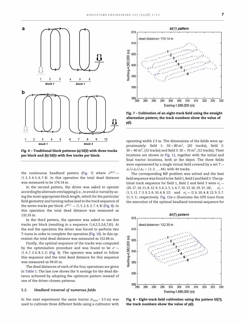
Fig. 7 – Cultivation of an eight-track field using the straight

alternation pattern; the track numbers show the value of

p(i).

Fig. 6 – Traditional block patterns (a) bl(3) with three tracks

per block and (b) bl(5) with five tracks per block.

Fig. 8 – Eight-track field cultivation using the pattern bl(7);

the track numbers show the value of p(i).

b i o s y s t e m s e n g i n e e r i n g 1 0 1 ( 2 0 0 8 ) 1 – 1 2 7

the continuous headland pattern (Fig. 7) where sblð1Þ ¼C1; 2;3;4; 5; 6;7;8D. In this operation the total dead distance

was measured to be 174.14 m.

In the second pattern, the driver was asked to operate

according by alternate overlapping (i.e., to avoid U-turns) by us-

ing the most appropriate block length, which for the particular

field geometry and turning radius lead to the track sequence of

the seven tracks per block: sblð7Þ ¼ C1; 5;2;6; 3; 7;4;8D (Fig. 8). In

this operation the total dead distance was measured as

132.35 m.

In the third pattern, the operator was asked to use five

tracks per block (resulting in a sequence C1,4,2,5,3,6,7,8D). At

the end the operation the driver was forced to perform two

T-turns in order to complete the operation (Fig. 10). In this op-

eration the total dead distance was measured as 152.84 m.

Finally, the optimal sequence of the tracks was computed

by the optimisation procedure and was found to be s� ¼C1; 4;7;3; 6; 8;5;2D (Fig. 9). The operator was asked to follow

this sequence and the total dead distance for this sequence

was measured as 99.65 m.

The dead distances of each of the four operations are given

in Table 1. The last row shows the % savings for the dead dis-

tance achieved by adopting the optimum pattern instead of

one of the driver-chosen patterns.

5.2. Headland traversal of numerous fields

In the next experiment the same tractor (rmin¼ 3.5 m) was

used to cultivate three different fields using a cultivator with

operating width 2.5 m. The dimensions of the fields were ap-

proximately: field 1: 50� 80 m2, (20 tracks), field 2:

30� 40 m2, (12 tracks) and field 3: 30� 70 m2, (12 tracks). Their

locations are shown in Fig. 11, together with the initial and

final tractor locations, both at the depot. The three fields

were represented by a single virtual field covered by a set T ¼D1WD2WD3 ¼ f1; 2;.;44g with 44 tracks.

The corresponding BIP problem was solved and the best

field sequence was found to be: field 1, field 2 and field 3. The op-

timal track sequence for field 1, field 2 and field 3 were s�1 ¼C20; 17;14;11;8;12;9;3; 6; 2;5;1;4; 7;10; 13; 16;19;15;18D, s�2 ¼C1;5;11;7;3; 9; 2;6;10;4;8;12D and s�3 ¼ C2; 6;10; 4;8;12;9;3;7;

11;5; 1D, respectively. Fig. 12a–c illustrates the GPS trace from

the execution of the optimal headland traversal sequence for

Fig. 9 – The Eight-track field cultivation using the optimal

sequence; the track numbers show the value of p(i).

Table 1 – Measured dead distances during turnings forfour different patterns

Pattern s* sbl(1) sbl(7) sbl(5)

Dead distance (m) 99.65 174.14 132.35 152.84

Savings (%)a – 42.8 24.7 34.8

a JðsblÞ � Jðs�Þ=JðsblÞ � 100%.

b i o s y s t e m s e n g i n e e r i n g 1 0 1 ( 2 0 0 8 ) 1 – 1 28

each field. The total path is optimal in the sense that it

minimises the total non-working distance travelled during

headland turnings and out-of-the field distance (from the

depot to the first field, from one field to the other, and from

the last field back to the depot).

When themachine operatorwasaskedto usehisown judge-

ment, he visited the fields in the same sequence, but the track

sequences he followed for covering each field were as follows:

sdr1 ¼ sblð19Þ ¼ C1; 11;2;12;3; 13; 4;14;5; 15; 6;16;7;17; 8;18;9;19;

10;20D and sdr2 ¼ sdr

3 ¼ sblð11Þ ¼ C1; 7; 2;8;3;9; 4; 10;5;11; 6; 12D.

The non-working travelled distances measured during the

headlands turnings for all fields and for both traversal

sequences (algorithmic and operator-selected) are given in

Table 2. The last column shows the % savings for the measured

Fig. 10 – Eight-track field cultivation using the overlapping

alternation pattern; the track numbers show the value of

p(i).

turning distances using the optimal and driver-chosen

sequences, i.e., the ratio of the turning distance difference

over the turning distance using the driver-chosen pattern.

5.3. Comparison of theoretical and measured savings

Given an arbitrary track traversal sequence and an optimal

sequence, the turning distance savings can be computed

theoretically, using Eq. (3) to compute the corresponding total

turning distances. The savings reported in the previous exper-

iments were based on measurements from a set of experiment

instances. In order to compare the theoretical or predicted vs.

the measured savings when using optimal patterns instead

of traditional ones, three cultivations were performed on three

fields A, B, C, with different operating width for each field. The

operating width was 3 m in field A, 4.5 m in field B and 6 m in

field C. The total width of each field was such that the tractor

covered 40 tracks. Hence, field A was 120 m wide, field B

180 m, and field C 240 m. The best driver-chosen block pattern

was selected for each field. Field A was covered with a pattern

of 5 tracks per block: sblð5Þ ¼ C 1;4;2;5; 3zfflfflfflfflfflfflffl}|fflfflfflfflfflfflffl{

;6; 9;7;10;8zfflfflfflfflfflfflfflffl}|fflfflfflfflfflfflfflffl{

;.D, field B

with three tracks per block: sblð3Þ ¼ C 1;3;2zfflffl}|fflffl{

;4;6;5zfflffl}|fflffl{

;7;9; 8zfflffl}|fflffl{

;.D

and field C with the continuous pattern: sblð1Þ ¼ C1; 2;3;.D. In

each field the driver was asked to follow the corresponding

driver-chosen block pattern and the optimal pattern computed

by the optimisation.

Fig. 11 – Locations of the three dispersed fields for the

cultivation operation.

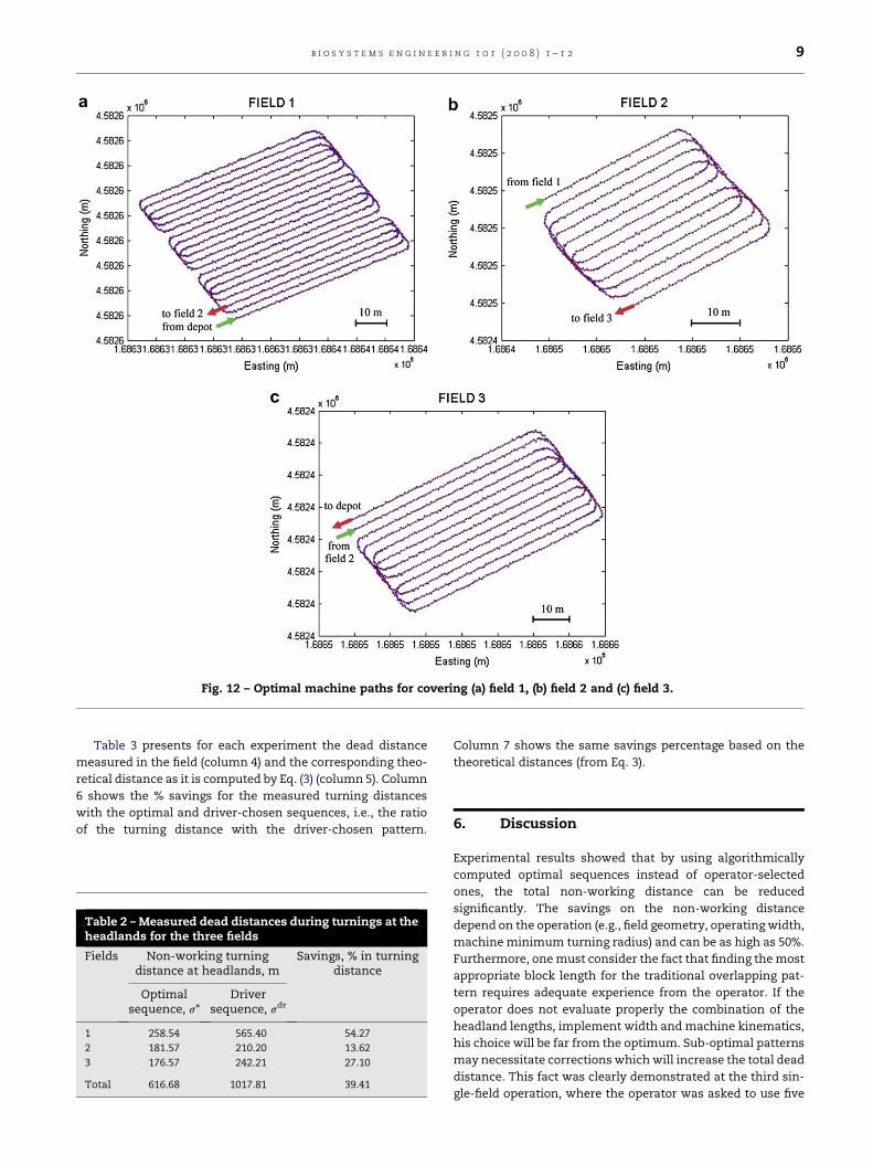
Fig. 12 – Optimal machine paths for covering (a) field 1, (b) field 2 and (c) field 3.

b i o s y s t e m s e n g i n e e r i n g 1 0 1 ( 2 0 0 8 ) 1 – 1 2 9

Table 3 presents for each experiment the dead distance

measured in the field (column 4) and the corresponding theo-

retical distance as it is computed by Eq. (3) (column 5). Column

6 shows the % savings for the measured turning distances

with the optimal and driver-chosen sequences, i.e., the ratio

of the turning distance with the driver-chosen pattern.

Table 2 – Measured dead distances during turnings at theheadlands for the three fields

Fields Non-working turningdistance at headlands, m

Savings, % in turningdistance

Optimalsequence, s*

Driversequence, sdr

1 258.54 565.40 54.27

2 181.57 210.20 13.62

3 176.57 242.21 27.10

Total 616.68 1017.81 39.41

Column 7 shows the same savings percentage based on the

theoretical distances (from Eq. 3).

6. Discussion

Experimental results showed that by using algorithmically

computed optimal sequences instead of operator-selected

ones, the total non-working distance can be reduced

significantly. The savings on the non-working distance

depend on the operation (e.g., field geometry, operating width,

machine minimum turning radius) and can be as high as 50%.

Furthermore, one must consider the fact that finding the most

appropriate block length for the traditional overlapping pat-

tern requires adequate experience from the operator. If the

operator does not evaluate properly the combination of the

headland lengths, implement width and machine kinematics,

his choice will be far from the optimum. Sub-optimal patterns

may necessitate corrections which will increase the total dead

distance. This fact was clearly demonstrated at the third sin-

gle-field operation, where the operator was asked to use five

Table 3 – Theoretical and measured dead distances and corresponding savings

Comparison Pattern Operatingwidth, m

Measured dead distance, m,J ¼

P39i¼1ðLminðdiÞ þ 3di

ÞTheoretical dead distance, m,

J ¼P39

i¼1 LminðdiÞSavings

measured, %Savings

theoretical, %

A Optimal 3 J(s*)¼ 618.25 J(s*)¼ 554.25 35.84 34.66

Traditional J(sbl(5))¼ 963.65 J(sbl(5))¼ 848.32

B Optimal 4.5 J(s*)¼ 599.36 J(s*)¼ 542.31 28.95 26.70

Traditional J(sbl(3))¼ 843.65 J(sbl(3))¼ 739.82

C Optimal 6 J(s*)¼ 674.53 J(s*)¼ 650.40 32.87 29.60

Traditional J(sbl(1))¼ 1004.83 J(sbl(1))¼ 923.88

b i o s y s t e m s e n g i n e e r i n g 1 0 1 ( 2 0 0 8 ) 1 – 1 210

tracks per block. This pattern proved to be inappropriate,

because at the end of the field the driver was forced to perform

two T-turns in order to complete the operation (Fig. 10). A big-

ger problem could arise in cases where there is not adequate

space for an U-turn. For example, an implement such as

a cultivator may reversing impractical. In such cases the

driver would have to manoeuvre the machine inside the field

interior.

Beyond the minimising the non-working distance when

turning a machine, the algorithmically computed optimal se-

quences also minimise the out-of-field travelled distance. For

example, when operating in the single-field experiments, the

optimal sequence caused the machine to start its operation

from track 1 and complete it after traversing track 2 (Fig. 9).

This makes sense, since the machine had to complete the

route ‘‘barn-field-barn’’ and so, it had to enter to the field

and exit the field from as close as possible to the barn (track

1). This fact can also be noticed at the numerous field opera-

tions experiment (Fig. 11). As illustrated in Fig. 12a, according

to the optimum path the machine had to start from the depot

and enter the first field close to its southern corner. After

covering field 1, it had to exit the field again close to its south-

ern corner and drive to field 2. For the operation in field 2 the

machine had to enter and exit the field from opposite sides of

the field (Fig. 12b). Finally, for field 3 (Fig. 12c) the machine had

to enter and exit the field from the western field tracks (tracks

1 and 2). The reason was that the starting location for the

route (the last track of field 2) and the final location (the depot)

were located both at the west side of the field. Notice that the

entry and exit tracks for each field are computed

automatically by the optimisation. In the case of the driver-

chosen pattern, as it appears from the sequence sdr1 , the driver

started the operation in field 1, from track 1, which was

located at the north side of the field. So, the tractor had to

travel across the field headland without operating. Similarly,

after operating in field 3, he travelled across the headland in

order to reach the depot. So, in this case a distance equal to

the sum of the lengths of the two headlands (about 80 m)

was travelled, more than with the optimal patterns.

A point that has to be noticed is the absence of any U-turns

with the optimal patterns. This fact leads to two significant

benefits that arise from the adoption of the optimal patterns.

The first is reduced soil disturbance because smooth P-turns

result in smaller lateral forces during manoeuvring. The sec-

ond benefit is a reduction in the headland area itself. Due to

the larger space that is required to execute U-turns, the

absence of this kind of turns decreases the required space at

the headlands. Furthermore, the optimal solution for most

problem instances is not unique, i.e., different track

sequences may minimise the total turning distance. These

solutions are generated randomly from the algorithms that

are usually used for this kind of optimisation problems.

Hence, the execution of such randomly generated optimal

patterns may lead to a more ‘‘fairly’’ distributed compaction

at the headlands than the repeated execution of the same

pattern over the years.

Regarding the comparison of theoretical and experimental

savings, as it was expected the theoretical turning distance

was always shorter than the measured one, for any traversal

pattern; yet, their difference was relatively small (3.6–12%).

This small difference arises mainly from the driver’s inability

to execute perfect shaped turn and the interaction between

soil and vehicle dynamics. The closeness of the theoretically

and experimentally measured turning distances implies that

Eq. (3) can be used to compute a reasonable approximation

of the turning distances, i.e., the cumulative distance term

(P39

i¼1 edi) is small. The measured savings in dead distance

were very close to the theoretical ones (in the order of 1.18,

2.25 and 3.27 for the corresponding operations in fields A, B

and C, respectively) because the approximation termP39

i¼1 edi

is small and it is also present in both the numerator and de-

nominator of the savings ratio.

7. Conclusions

An algorithmic approach for computing traversal sequences

for an agricultural machine operating in parallel tracks has

been developed. The computed sequences are optimal in the

sense that they minimise the total non-working distance trav-

elled. Field coverage was expressed as the traversal of

a weighted graph and the problem of finding an optimal tra-

versal sequence was shown to be equivalent to finding the

shortest tour in the graph. The optimisation was formulated

and solved as a BIP problem.

Experimental results showed that by using algorithmically

computed optimal sequences instead of operator-selected

ones, the total non-working distance could be reduced by up

to 50% depending on the operation. The reduction of non-

working distance entails equivalent reduction of the fuel

consumption as well as of the non-productive time. Moreover,

apart from improved efficiency, the adoption of optimal head-

land patterns may also lead to reduced soil compaction in the

headland area. The optimal patterns consist mainly of

P-turns and fewer – if any – U-turns. The smooth P-turns

b i o s y s t e m s e n g i n e e r i n g 1 0 1 ( 2 0 0 8 ) 1 – 1 2 11

result in smaller lateral forces during manoeuvring and conse-

quently in less compaction.

Beyond the reduction of the soil compaction at the head-

land area, the proposed optimal patterns reduce the headland

area itself. Due to the larger space that is required for the

execution of U-turns, the absence of this kind of turns

decreases the proportion of the field area that constitutes

the headland area and consequently the proportion of the

low productivity area, resulting in economic benefits.

The optimal track sequences are often counter-intuitive for

human operators. However, the programmable navigation-

aid systems supported by the terminals or auto-steering

systems which have been developed in recent years make it

feasible for a vehicle to follow arbitrary optimal patterns. In

addition to its application in present day navigation systems,

this technique is directly applicable to route planning of

autonomous agricultural vehicles.

Appendix.Extension to numerous fields

The traversal graph can be easily extended to model the cov-

erage of numerous separate fields, each covered by a headland

pattern. Consider k fields arbitrarily numbered from 1 to k,

with the ith field covered by a set of tracks Ti ¼ f1; 2;.; kTikg.The union of all tracks can be thought of as a ‘virtual’ field

which is covered by a set of tracks T ¼ D1WD2W/WDk where

the set Di represents the same tracks as Ti with an appropriate

offset in their indexing, i.e.,

Di ¼

8<:X

i�1

j¼1

��Tj

��þ 1;Xi�1

j¼1

��Tj

��þ 2;.Xi

j¼1

��Tj

��9=;; i ¼ 1;.; k (13)

for example, if T1 ¼ f1;2;3g and T2 ¼ f1;2g then D1 ¼ f1;2;3gand D2 ¼ f3þ 1;3þ 2 ¼ f4; 5gg , respectively, and T ¼f1; 2; 3;4;5g.

The extended traversal graph G0 for the virtual field is

defined exactly as the graph for the single-field case. It

contains all the nodes in the track set, T, the nodes which

correspond to the initial and final position, and the set of

arcs, A, which connect all nodes. However, the cost cij

associated with arc Aij must be calculated differently,

depending on whether tracks i and j belong to the same field

or not. If they do, then cij is equal to the turning cost Lmin(dij),

just as in the single-field case. Otherwise, the cost of going

from the end of track i in a field a, to the beginning of track

j in a field b, depends on the relative position of the different

fields a, and b, and the positions of the tracks in their

respective field.

In principle, one could calculate these costs exactly based

on geometry and on the dynamics of the machine. Let Dab be

the Euclidean distance between the beginning of the first

track of field a, and the beginning of the first track of field

b; obviously Dab¼Dba. In typical situations, this inter-field

distance is much larger than the distance between any two

tracks of the same field and orders of magnitude larger

than the turning radius of the machine. Therefore, for all

practical purposes it should suffice to assign the costs cij

based on estimates of straight-line distances. Such an esti-

mate is given next.

When track i belongs to field a and track j belongs to field b,

the cost cij is set equal to the inter-field distance Dab plus two

signed terms which account for the distance (in multiples of

the operating width, w) of track i from the first track in field

a, and the distance of track j from the first track of field b,

respectively:

cij ¼DabHw$

"i�

1þXa�1

m¼1

kTmk!#�w$

"j�

1þXb�1

m¼1

kTmk!#

(14)

in the above expression the terms 1þPx�1

m¼1 kTmk correspond to

the number of the first track in Dx. The upper signs are used

when a< b, i.e., field a, comes before field b in the arbitrarily

numbered field sequence (e.g., a¼ 2, b¼ 4), whereas the lower

signs are used when a> b. The sign change can be expressed

algebraically as ða� bÞ=ja�bj. To summarise, the cost cij is

given by:

cij ¼

8><>:

Lminðji� jjÞ; if a¼ b

Dabþ a�bja�bjw

�i�� Pa�1

m¼1kTmkþ 1

�

�"

j� Xb�1

m¼1

kTmkþ 1

!#); if asb: ð15Þ

Again, it is assumed that the graph contains at least one se-

quence of nodes connecting node 0 to node kTkþ1 with finite

cost, i.e., that there is at least one feasible traversal sequence

connecting all tracks in all fields.

r e f e r e n c e s

Ansorge D; Godwin R J (2007). The effect of tyres and a rubbertrack at high axle loads on soil compaction. Part 1: single axlestudies. Biosystems Engineering, 98(1), 115–126.

ASAE. (2005). ASAE S495.1 NOV2005. Uniform Terminology forAgricultural Machinery Management. ASABE, St. Joseph,Michigan.

Bailey J (1997). Tractor-based systems for traffic control in arablecrops. Landwards, 52(2), 2.

Benson E R; Hansen A C; Reid J F; Warman B L; Brand M A(2002). Development of an In-field Grain Handling Simulationin ARENA. ASAE Paper No. 02-3104. ASAE, St. Joseph,Michigan.

Blackmore B S; Griepentrog H W (2006). Autonomous vehicles androbotics, In: CIGR Handbook of Agricultural Engineering, Vol.VI, pp 204–215.

Bochtis D; Vougioukas S; Tsatsarelis C (2006). A vehicle routingproblem formulation of agricultural field operations planningfor self-propelled machines, In: XVI CIGR Word Congress,Bonn, Germany. Abstract in Book of Abstracts, pp 301–302,(Full paper on CD 6pp).

Clarke G; Wright J (1964). Scheduling of vehicles from a centraldepot to a number of delivery points. Operations Research,12(4), 568–581.

Dudek G; Jenkin M (2000). Computational Principles of MobileRobotics. Cambridge University Press.

Garey M; Johnson D (1979). Computers and Intractability: a Guideto the Theory of NP-Completeness. Freeman, San Francisco,CA, USA.

Glover F; Kochenberger G (2002). Handbook of Metaheuristics.Kluwer Academic Publishers, Norwell, MA, USA.

Gutin G; Punnen A (2007). The Traveling Salesman Problem andIts Variations. Springer.

b i o s y s t e m s e n g i n e e r i n g 1 0 1 ( 2 0 0 8 ) 1 – 1 212

Hansen A C; Hornbaker R H; Zhang Q (2003). Monitoring and analysisof in-field grain handling operations. ASEA Paper No 701P1103e.Proceedings of International Conference on Crop Harvesting,Louisville, Kentucky, USA. ASAE, St. Joseph, Michigan.

Hunt D (2001). Farm Power and Machinery Management (tenthed.). Iowa State Press, Ames, Iowa.

Keicher R; Seufert H (2000). Automatic guidance for agriculturalvehicles in Europe. Computers and Electronics in Agriculture,25, 169–194.

Keller T (2005). A model for the prediction of the contact area and thedistribution of vertical stress below agricultural tyres from readilyavailable tyre parameters. Biosystems Engineering, 92(1), 85–96.

Oksanen T (2007). Path planning algorithms for agricultural fieldmachines. PhD Thesis, Helsinki University of TechnologyAutomation, Technology Laboratory, Finland.

Reid J F; Zhang Q; Noguchi N; Dickson M (2000). Agriculturalautomatic guidance research in North America. Computersand Electronics in Agriculture, 25, 155–167.

Snyder L; Daskin M (2004). A Random-Key Genetic Algorithm forthe Generalized Traveling Salesman Problem. Technical

Report #04T-018. Department of Industrial & SystemsEngineering, Lehigh University.

Sørensen C G; Bak T; Jorgensen R N (2004). Mission planner foragricultural robotics, In: AgEng 2004, Leuven, Belgium, 12–16September 2004. Abstract in Book of Abstracts, pp 894–895(Full paper on CD 8pp).

Taylor R K; Schrock M D; Staggenborg S A (2002). ExtractingMachinery Management Information from GPS Data. ASAE, St.Joseph, Michigan. Paper No. 02-10008.

Witney B (1996). Choosing and Using Farm Machines. LandTechnology, Edinburgh.

Wolsey L A (1998). Integer Programming. John Wiley and Sons,New York.

Vougioukas S; Blackmore S; Nielsen J; Fountas S (2006). A two-stage optimal motion planner for autonomous agriculturalvehicles. Precision Agriculture, 7, 361–377.

Zhang Q; Reid J F; Noguchi N (1999). Agricultural vehiclenavigation using multiple guidance sensors, In:Proceedings of International Conference on Field andService Robotics.