Ann Inst Stat Math (2015) 67:673–685DOI 10.1007/s10463-014-0470-0

Minimax design criterion for fractional factorial designs

Yue Yin · Julie Zhou

Received: 12 November 2013 / Revised: 15 March 2014 / Published online: 18 May 2014© The Institute of Statistical Mathematics, Tokyo 2014

Abstract An A-optimal minimax design criterion is proposed to construct fractionalfactorial designs, which extends the study of the D-optimal minimax design criterionin Lin and Zhou (Canadian Journal of Statistics 41, 325–340, 2013). The resulting A-optimal and D-optimal minimax designs minimize, respectively, the maximum traceand determinant of the mean squared error matrix of the least squares estimator (LSE)of the effects in the linear model. When there is a misspecification of the effectsin the model, the LSE is biased and the minimax designs have some control overthe bias. Various design properties are investigated for two-level and mixed-levelfractional factorial designs. In addition, the relationships amongA-optimal,D-optimal,E-optimal, A-optimal minimax and D-optimal minimax designs are explored.

Keywords A-optimal design · D-optimal design · Factorial design ·Model misspecification · Requirement set · Robust design

1 Introduction

Factorial designs are very useful in industrial experiments to investigate possible influ-ential factors. A full factorial design allows us to examine all the main effects andinteractions among the factors. However, the total number of runs in a full factorialdesign can be huge for a large number of factors, and often there may not be enoughresources to run it. In this situation, a fractional factorial design (FFD) can be applied,although it does not allow us to estimate all the main effects and interactions. There area couple of ways to deal with this. One way is to assume that higher-order interactionsare negligible, and we only estimate lower-order effects. Another way is to specify and

Y. Yin · J. Zhou (B)Department of Mathematics and Statistics, University of Victoria, Victoria, BC V8W 2Y2, Canadae-mail: jzhou@uvic.ca

123

674 Y. Yin, J. Zhou

analyze a subset of possible significant effects. The subset is referred as a requirementset that usually contains all the main effects and some interactions. In this paper, weconstruct optimal/robust FFDs for given requirement sets.

Suppose N is the run size of a full factorial design, and n is the affordable run sizewith n < N . There are

(Nn

)possible choices to choose a FFD. Which one should we

choose? Various optimal criteria have been explored in the literature. For example, seeMukerjee and Wu (2006) for regular FFD criteria based on the component hierarchyprinciple, and developments for nonregular FFDs are reviewed in Xu et al. (2009).

The commonly used A-, D- and E-optimal design criteria are model based. Theyhave been investigated extensively in the literature, and optimal designs have beenconstructed for various regression models. For example, see Fedorov (1972) andPukelsheim (1993). These criteria can also be applied to select optimal FFDs. InTang and Zhou (2009, 2013), D-optimal designs for two-level FFDs are studied forvarious requirement sets and run sizes.

If the requirement set includes all the significant effects of the factors in the exper-iment, then the bias of the least squares estimator (LSE) is negligible. However, therequirement set may not be correctly specified, and in particular it may miss some sig-nificant effects.When this happens, the bias of the LSE is not negligible and needs to beconsidered in the construction of optimal FFDs. This motivated the research inWilmutand Zhou (2011), where a D-optimal minimax criterion was proposed for two-levelfactorial designs. A D-optimal minimax design (DOMD) minimizes the maximumdeterminant of the mean squared error (MSE) of the LSE, and the maximum is takenover small possible departures of the requirement set. Lin and Zhou (2013) extendedthis criterion tomixed-level factorial designs and derived several interesting propertiesof DOMDs. These designs are robust against misspecification of the requirement setwhich is similar to the misspecification in the regression response function. The biasof the LSE is also the focus in minimum aberration designs, which have been studiedby many authors including Cheng and Tang (2005).

In this paper, the minimax approach is further extended to the A-optimal minimaxcriterion, and properties of A-optimal minimax FFDs are explored. In addition, therelationships among A-optimal, D-optimal, E-optimal, A-optimal minimax and D-optimal minimax designs are investigated and several theoretical results are obtained.

2 Notation

Consider a full factorial design for k factors, F1, F2, . . . , Fk , witha1, a2, . . . , ak levels,respectively. The total number of runs is N = a1a2 · · · ak . In this paper, all the maineffects and interactions are coded to be orthogonal when we fit a full linear model toestimate those effects. There are N − 1 coded variables in the model and denoted byx1, x2, . . . , xN−1. Let U be the N × N model matrix of the full model, and its firstcolumn is a vector of ones 1N for the grand mean term.

A FFD of n runs is selected from the N rows of U without replacement. The FFDshould allow us to estimate all the effects in a requirement set R. Since the columnsof U can be permuted, without loss of generality, we assume that the first q variablesx1, . . . xq represent all the effects inR. For the i th run in the FFD, those variables take

123

Minimax design criterion 675

values as xi1, . . . xiq , which comes from a selected row of U. Then the linear modelforR is, yi = θ0 + θ1xi1 + . . . + θq xiq + εi , i = 1, . . . , n, where yi is the observedresponse at the i th run, and the errors εi ’s are assumed to be i.i.d. with mean 0 andvariance σ 2. Let X1 be the model matrix, y = (y1, . . . , yn)�, θ1 = (θ0, θ1, . . . , θq)

�,and ε = (ε1, . . . , εn)

�. Then the model can be written in a matrix form as

y = X1θ1 + ε. (1)

The LSE of θ1 is θ̂1 = (X�1 X1

)−1X�1 y, and Cov(θ̂1) = σ 2

(X�1 X1

)−1.

Partition matrix U into U = (U1,U2), where U1 contains the column 1N and thecolumns for variables x1, . . . , xq , and U2 contains the others. Since the columns of Uare orthogonal, we have

U�U =(U�1 U1 U�

1 U2

U�2 U1 U�

2 U2

)

=(V1 00 V2

), (2)

where both V1 = U�1 U1 and V2 = U�

2 U2 are diagonal matrices.If R misses some significant effects, then model (1) is misspecified. A possible

model with small departures from (1) is derived in Lin and Zhou (2013), which canbe written as y = X1θ1 + X2θ2 + ε, where X2 is the model matrix for variablesxq+1, . . . , xN−1, and θ2 = (θq+1, . . . , θN−1)

� is an unknown parameter vector sat-isfying 1

N θ�2 V2θ2 ≤ α2. Here α ≥ 0 controls the size of departures. When α = 0,

model (1) is assumed to be correct. It is clear that X1 and X2 are submatrices of U1and U2, respectively.

3 Design criteria

Commonly used A-optimal, D-optimal, and E-optimal criteria are based on mea-sures of the covariance matrix of the LSE. In particular, the A-optimal design(AOD), D-optimal design (DOD), and E-optimal design (EOD) minimize the trace,the determinant and the largest eigenvalue of Cov(θ̂1), respectively. However, ifmodel (1) is misspecified, then the LSE θ̂1 is biased with bias (θ̂1) = E(θ̂1) − θ1 =(X�1 X1

)−1X�1 X2θ2. The MSE is

MSE (θ̂1,X1, θ2) =(X�1 X1

)−1X�1 X2θ2θ

�2 X

�2 X1

(X�1 X1

)−1 + σ 2(X�1 X1

)−1.

(3)

Consider the loss function LDM(X1) = maxθ2∈� det(MSE(θ̂1,X1, θ2)

), where

� = {θ2 | 1

N θ�2 V2θ2 ≤ α2

}. Then the design minimizing LDM(X1) over all pos-

sible designs X1 is called a DOMD, which has been investigated in Wilmut and Zhou(2011) and Lin and Zhou (2013).

123

676 Y. Yin, J. Zhou

Similar to theD-optimalminimaxcriterion,wenowpropose theA-optimalminimaxcriterion based on the trace of the MSE as follows. Define a loss function

LAM(X1) = maxθ2∈�

trace(MSE(θ̂1,X1, θ2)

), (4)

and an A-optimal minimax design (AOMD) minimizes LAM(X1) over X1.Both AOMDs and DOMDs are robust against misspecification of the requirement

set. It looks like we need to solve minimax problems to find AOMDs and DOMDs.Since the analytical expressions for LAM(X1) and LDM(X1) can be derived, we onlyneed to solve minimization problems. Thus, it is not more difficult to find AOMDsand DOMDs than AODs and DODs. The expression for LDM(X1) is,

LDM(X1) = σ 2(q+1)1 + Nα2

σ 2

(1 − λmin

(V−1/21 X�

1 X1V−1/21

))

det(X�1 X1

) , (5)

where λmin() is the smallest eigenvalue of a matrix, from Lin and Zhou (2013). Theanalytical expression for LAM(X1) is obtained in the next theorem.

Theorem 1 The loss function in (4) equals to

LAM(X1) = σ 2{trace

((X�1 X1

)−1)

+ Nα2

σ 2 λmax

((X�1 X1

)−1 − V−11

)}, (6)

where λmax() denotes the largest eigenvalue of a matrix.

The proof of Theorem 1 is in the Appendix. This result is very useful to exploretheoretical properties of AOMDs and find relationships with other optimal designs.From (5) and (6), it is clear that DOMDs and AOMDs depend on parameter α2 onlythrough a parameter v = α2/σ 2, which can be viewed as the bias to variance ratio. Ifthe bias is not important, choose v close to zero. Some optimal designs do not dependon v, and detailed results and comments are given in Sects. 4 and 5.

Theorem 2 For a given requirement set, the minimum loss for AOMDs,minX1 LAM(X1), is a nonincreasing function of n.

The proof of Theorem 2 is in the Appendix. Similar results have been proved forother optimal designs, such as DOMDs in Lin and Zhou (2013).

4 Results for two-level designs

For a two-level factor, “+1” and “−1” are used to code the high and low levels. Allthe regression variables x1, . . . , xN−1 take values ±1 and are orthogonal for a fullfactorial design. Thus, from (2), matrix V1 = N Iq+1 with N = 2k , and the lossfunctions in (5) and (6) become,

123

Minimax design criterion 677

LDM(X1) = σ 2(q+1) 1 + v(N − λmin

(X�1 X1

))

det(X�1 X1

) , (7)

LAM(X1) = σ 2

{

trace

((X�1 X1

)−1)

+ v

(N

λmin(X�1 X1

) − 1

)}

. (8)

Also AOD, DOD and EOD minimize the following loss functions, respectively,

LA(X1) = σ 2trace

((X�1 X1

)−1)

, LD(X1) = σ 2(q+1)

det(X�1 X1

) ,

LE (X1) = 1

λmin(X�1 X1

) .

If v = 0, then there is no bias and the loss functions in (7) and (8) are the same as thosefor D-optimal and A-optimal criteria, respectively. In general, we have the followingrelationships,

LDM(X1) = LD(X1)

(1 + v

(N − 1

LE (X1)

)),

LAM(X1) = LA(X1) + α2 (NLE (X1) − 1) .

From these relationships, it is obvious that

(1) If a design is both DOD and EOD, then it is a DOMD for all values of v.(2) If a design is both AOD and EOD, then it is an AOMD for all values of α2.(3) If α2 = 0, then a DOMD is a DOD and an AOMD is an AOD.(4) For large α2 and v, an EOD tends to be a DOMD and AOMD.

For a given requirement set R, a design X1 is said to be orthogonal for R if itsatisfies X�

1 X1 = n Iq+1. This definition of orthogonal design is slightly differentfrom the one in Tang and Zhou (2009) and other papers, where an orthogonal designimplies that the main effects are orthogonal. Here orthogonal designs for R make allthe effects in R orthogonal, so they are more restricted than the orthogonal designsfor main effects only.

Lemma 1 An orthogonal design forR is an AOD, DOD, EOD, AOMD and DOMD.

It is well anticipated from the results on universal optimality for full rank models(Sinha andMukerjee 1982). This result shows that optimal designs can be constructedby finding orthogonal designs for R if they exist. However, for many run sizes of nand requirement setsR, orthogonal designs forR do not exist. For example, if n is nota multiple of 4, orthogonal designs do not exist for any R with q ≥ 2. Next theoremshows another result that orthogonal designs do not exist.

Theorem 3 Orthogonal designs for R do not exist for run size n ∈ [N − q, N − 1],where q is the number of effects in R.

123

678 Y. Yin, J. Zhou

The proof of Theorem 3 is in the Appendix. This result indicates that orthogonaldesigns forR do not exist if the run size is close to N − 1. Orthogonal designs forRmay not exist even when n is a multiple of 4 and is small. For example, if n is not amultiple of 8, e.g.,n = 12 or 20, and R includes some two-factor interactions and/orthree-factor interactions, then orthogonal designs for R do not exist from Deng andTang (2002, Proposition 1).

If the regressors x1, · · · , xN−1 aremultiplied by constant nonzero numbers b1, · · · ,

bN−1, respectively, do optimal designs stay the same? This is a scale invariant issue.DODs are known to be scale invariant. Lin and Zhou (2013) also proved that DOMDsare scale invariant. However, AODs are not scale invariant. Since AODs are AOMDswhen v = 0, AOMDs are not scale invariant either. Nevertheless, this lack of scaleinvariance is not amatter of concern becauseAODs andAOMDs are usedwhen interestlies in the parameters as they stand and not in their multiplies or linear transformations.

Another property is the level-permutation invariance. DODs and DOMDs are level-permutation invariant (Lin and Zhou 2013) for a special class of permutations. Fortwo-level designs, there is only one level permutation: switching the two levels (highlevel ↔ low level). It turns out that AODs and AOMDs are also level-permutationinvariant, which is a result of the next theorem.

Theorem 4 Let X̃1 = X1Q, where Q is a diagonal matrix with diagonal elementsbeing ±1. Then we have LAM(X̃1) = LAM(X1), where function LAM is given in (8).

The proof of Theorem 4 is straight forward and is omitted. If a factor’s two levelsare permuted, then the corresponding main effect variable and interaction variablesinvolving this factor change a sign. Therefore, we have X̃1 = X1Q, where X1 and X̃1are the model matrices before and after the permutation, and the diagonal elementsof Q are ±1. The result in Theorem 4 implies that AOMDs are level-permutationinvariant. This result can have the following two interpretations:

(1) It does not matter how we label the two levels as high and low levels. It is veryhelpful in practice, since the high and low levels are not clear for categoricalfactors, such as tool type or material type.

(2) AOMDs are not unique. Switching the levels of one or more factors in an AOMDyields another AOMD.

The following two examples will show the properties for two-level designs. Sinceoptimal designs do not depend on the value of σ 2, it is set to be 1 in all the examples.

Example 1 Consider an experiment to investigate 4 factors and a requirement setR = {F1, F2, F3, F4, F1F2, F3F4}. For this R, we have N = 16 and q = 6. Weconstruct optimal designs for n = 8, 9, · · · , 15 to illustrate design properties discussedin this section. For each run size n, a complete search is done to find AODs, DODs,EODs, AOMDs and DOMDs. The following is the summary of the results.

(1) Orthogonal designs for R do not exist for any n ∈ [8, 15]. For 9 ≤ n ≤ 15, thisresult is obvious from Theorem 3 and the comments after Lemma 1. For n = 8,it is due to the specific structure of the effects inR.

(2) Optimal designs are not unique, which is consistent with the comments afterTheorem 4.

123

Minimax design criterion 679

Table 1 Optimal designs and minimum loss functions in Example 1

n Optimal designs LA LAM L1/(q+1)D L1/(q+1)

DM LE

8 1, 2, 5, 8, 10, 11, 15, 16 1.3750 7.2034 0.1524 0.2236 0.4268

9 1, 2, 3, 5, 8, 10, 12, 15, 16 1.0417 4.0417 0.1281 0.1848 0.2500

10 1, 2, 4, 5, 6, 9, 11, 14, 15, 16 0.9072 3.9072 0.1127 0.1626 0.2500

11 AOD, DOD and DOMD: 1, 2,3, 5, 6, 8, 9, 11, 12, 14, 15

0.7750 0.0993 0.1429

EOD and AOMD: 1, 2, 3, 5, 6, 8, 9, 11, 12, 13, 16 3.4237 0.2266

12 1, 2, 3, 5, 6, 8, 9, 11, 12, 14, 15, 16 0.6458 1.6458 0.0876 0.1200 0.1250

13 1, 2, 3, 4, 5, 6, 7, 9, 11, 12, 13, 14, 16 0.5909 1.5909 0.0804 0.1100 0.1250

14 1, 2, 3, 4, 5, 6, 7, 8, 9, 10, 11, 14, 15, 16 0.5375 1.5375 0.0738 0.1010 0.1250

15 1, 2, 3, 4, 5, 6, 7, 8, 9, 10, 11, 12, 13, 14, 15 0.4861 1.2639 0.0679 0.0913 0.1111

(3) All the optimal designs are equivalent when n = 9, 12, 13, 14, 15. As a result,AOMDs and DOMDs do not depend on the value of v. When n = 8 and 10,there are more EODs than the other optimal designs. AODs, DODs, AOMDs andDOMDs are equivalent, and they are all EODs. Thus, AOMDs and DOMDs donot depend on the value of v either. Some EODs are not AODs, DODs, AOMDsand DOMDs. When n = 11, AODs and DODs are different from EODs, soAOMDs and DOMDs depend on the value of v. For v = 1, AOMDs and EODsare equivalent, while DOMDs and DODs are the same.

(4) Table 1 presents the minimum loss functions and optimal designs. For LAM andLDM, the results are for v = 1. Since optimal designs are not unique, one designis given for each case. The numbers in the optimal designs are the run numbersfrom a full factorial design and generated as follows (Wilmut and Zhou 2011):the first run is for all the factors at level −1, then factor Fi alters between −1 and+1 for every 2i−1 runs, i = 1, 2, 3, 4. The results show that the loss functionsdecrease as n increases for all the criteria, which is consistent with Theorem 2.

Example 2 Consider a requirement set R = {F1, F2, F3, F4, F5, F1F2, F1F3} withN = 32 and q = 7. We construct optimal designs for n = 8, 12, 15, 16, 19, 20. Since(Nn

)can be huge, we apply the simulated annealing algorithm in Wilmut and Zhou

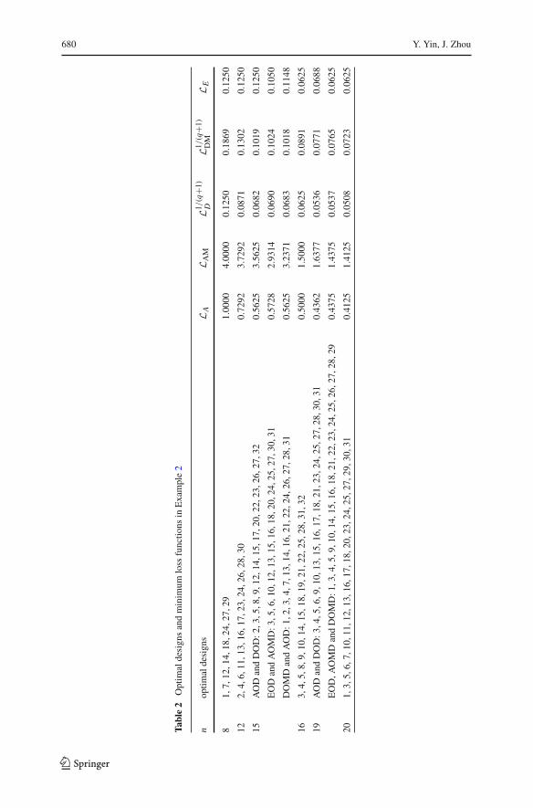
(2011) to search for the optimal designs. A simulated annealing algorithm is knownto be effective finding optimal designs and has been applied by many authors; seeother references and the detailed algorithm inWilmut and Zhou (2011). Table 2 showssome optimal designs and the minimum loss functions, over a wide class of designs ascovered by the simulated annealing algorithm. Here is the summary of the numericalresults, where AOMDs and DOMDs are computed for v = 1.

(1) Orthogonal designs forR exist for n = 8 and 16. In fact, many regular fractionalfactorial designs (25−2 and 25−1) are orthogonal designs for this R.

(2) For n = 8, 12, 16 and 20, all the optimal designs are equivalent.(3) For n = 15 and 19, the optimal designs are different. For n = 15, some AODs

are DODs, some EODs are AOMDs, and some DOMDs are AODs. For n = 19,

123

680 Y. Yin, J. Zhou

Table2

Optim

aldesign

sandminim

umloss

functio

nsin

Example2

nop

timaldesign

sL A

L AM

L1/(q

+1)

DL1

/(q

+1)

DM

L E8

1,7,12

,14,18

,24,

27,29

1.00

004.00

000.12

500.18

690.12

50

122,

4,6,

11,13,

16,17,23

,24,26

,28,

300.72

923.72

920.08

710.13

020.12

50

15AODandDOD:2

,3,5

,8,9,1

2,14

,15,

17,20,

22,23,26

,27,32

0.56

253.56

250.06

820.10

190.12

50

EODandAOMD:3

,5,6

,10,12

,13,

15,16,18

,20,24

,25,

27,30,31

0.57

282.93

140.06

900.10

240.10

50

DOMDandAOD:1

,2,3,4

,7,1

3,14

,16,21

,22,

24,26,27

,28,31

0.56

253.23

710.06

830.10

180.11

48

163,

4,5,

8,9,

10,14,

15,18,19

,21,22

,25,28

,31,

320.50

001.50

000.06

250.08

910.06

25

19AODandDOD:3

,4,5

,6,9,1

0,13

,15,

16,17,

18,21,23

,24,25

,27,

28,30,31

0.43

621.63

770.05

360.07

710.06

88

EOD,A

OMDandDOMD:1

,3,4,5

,9,1

0,14

,15,16

,18,

21,22,23

,24,25

,26,

27,28,29

0.43

751.43

750.05

370.07

650.06

25

201,

3,5,

6,7,

10,11,

12,13,16

,17,18

,20,23

,24,

25,27,29

,30,31

0.41

251.41

250.05

080.07

230.06

25

123

Minimax design criterion 681

Table 3 Orthogonal codes for athree-level factor

Factor level xL xQ

0 −1 +1

1 0 −2

2 +1 +1

some EODs are both AOMDs and DOMDs. AOMDs and DOMDs depend on thevalue of v.

5 Results for mixed-level designs

In this section, we consider designs with some factors taking more than two levels.The following two cases are discussed in detail, but the methodology is quite generaland can be applied to other cases.

Case 1: Factors have mixed two levels and three levels.Case 2: All the factors have three levels.A two-level factor is coded the same as in Sect. 4. A three-level factor needs two

variables to represent the main effect, and they are called the linear xL and quadraticxQ components and coded orthogonally as in Table 3.

For two-level designs, we have V1 = NIq+1, so the loss functions of AOMDsand DOMDs can be simplified and several nice properties about the optimal designshave been derived in Sect. 4. However, mixed-level designs usually do not have V1 =NIq+1, which makes it harder to obtain minimax design properties.

Consider a level permutation π , and let X1 and Xπ1 be the model matrices before

and after the permutation, respectively. The permutation can involve level changes inone or more factors. Define a class of permutations,

= {π | Xπ

1 = X1Qπ , where Qπ is a diagonal matrix with elements ± 1}.

Next theorem shows that AOMDs are invariant under the level permutations in .

Theorem 5 Let Xπ1 = X1Qπ , whereQπ is a diagonal matrix with diagonal elements

being ±1. Then, we have LAM(Xπ1 ) = LAM(X1), where function LAM is given in (6).

The proof of Theorem 5 is in the Appendix. This result is true for factors with anylevels. This includes the permutation for two-level factors discussed in Sect. 4 andthe permutation for three-level factors by switching levels 0 and 2. Next two examplespresent some AOMDs for mixed-level designs and their properties.

Example 3 Suppose there are three factors, F1, F2 and F3, and each has three levels.A requirement set includes all the main effects and the interaction between F1 andF2, i.e., R = {F1, F2, F3, F1F2} with N = 27 and q = 10. We construct AOMDsfor n = 21 and 24 using a complete search, and the results are presented in Tables 4and 5. For n = 21, there is only one AOD, and there are eight AOMDs. The AOD isdifferent from the AOMDs. All the eight AOMDs can be generated from the AOMD

123

682 Y. Yin, J. Zhou

Table 4 Optimal designs for n = 21 in Example 3

Factor Factor levels

AOD: LA = 0.5394

F1 0 1 2 0 2 0 1 2 0 2 1 0 2 0 1 2 0 2 0 1 2

F2 0 0 0 1 1 2 2 2 0 0 1 2 2 0 0 0 1 1 2 2 2

F3 0 0 0 0 0 0 0 0 1 1 1 1 1 2 2 2 2 2 2 2 2

AOMD: LAM = 1.5574

F1 0 2 0 1 2 0 2 1 2 0 1 1 2 0 1 2 0 2 0 1 2

F2 0 0 1 1 1 2 2 0 0 1 1 2 2 0 0 0 1 1 2 2 2

F3 0 0 0 0 0 0 0 1 1 1 1 1 1 2 2 2 2 2 2 2 2

Table 5 Optimal designs for n = 24 in Example 3

factor factor levels

AOD and AOMD: LA = 0.4595, LAM = 0.9595

F1 0 1 2 0 1 2 0 1 2 0 1 2 1 0 1 2 0 1 2 0 2 0 1 2

F2 0 0 0 1 1 1 2 2 2 0 0 0 1 2 2 2 0 0 0 1 1 2 2 2

F3 0 0 0 0 0 0 0 0 0 1 1 1 1 1 1 1 2 2 2 2 2 2 2 2

in Table 4 by permuting the levels 0 and 2 of F1 and F3 and by switching two factorsF1 and F2. Permuting the levels 0 and 2 of F2 does not generate more designs. Theconstruction through switching factor levels is from the result in Theorem 5, whilethe construction through switching two factors works because of the symmetry of therequirement setR in F1 and F2. For n = 24, all the AODs and AOMDs are the same.There are four AODs and AOMDs. Table 5 shows one of them, and the other threecan be generated by permuting the levels 0 and 2 of F3 and by switching two factorsF1 and F2.

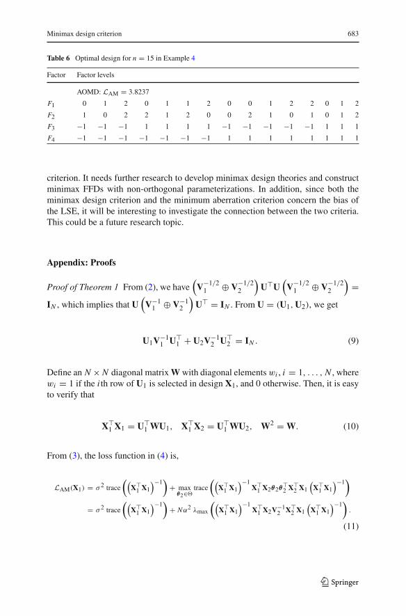
Example 4 Consider an experiment with four factors: F1 and F2 with three levels,and F3 and F4 with two levels. We want to estimate all the main effects, the inter-action between F1 and F3, and the interaction between F3 and F4, so requirementset R = {F1, F2, F3, F4, F1F3, F3F4}, N = 36 and q = 9. For each run sizen = 12, 15, 18, 20, 24 and 30, a simulated annealing algorithm is run 10 times andthe design with the smallest loss function is taken as an AOMD. Table 6 presents oneAOMD for n = 15.

6 Discussion

All the results are derived for an orthogonal parameterization in this paper. In practice,there are situations for a non-orthogonal parameterization, such as in Mukerjee andTang (2012), where two-level FFDs are constructed using the minimum aberration

123

Minimax design criterion 683

Table 6 Optimal design for n = 15 in Example 4

Factor Factor levels

AOMD: LAM = 3.8237

F1 0 1 2 0 1 1 2 0 0 1 2 2 0 1 2

F2 1 0 2 2 1 2 0 0 2 1 0 1 0 1 2

F3 −1 −1 −1 1 1 1 1 −1 −1 −1 −1 −1 1 1 1

F4 −1 −1 −1 −1 −1 −1 −1 1 1 1 1 1 1 1 1

criterion. It needs further research to develop minimax design theories and constructminimax FFDs with non-orthogonal parameterizations. In addition, since both theminimax design criterion and the minimum aberration criterion concern the bias ofthe LSE, it will be interesting to investigate the connection between the two criteria.This could be a future research topic.

Appendix: Proofs

Proof of Theorem 1 From (2), we have(V−1/21 ⊕ V−1/2

2

)U�U

(V−1/21 ⊕ V−1/2

2

)=

IN , which implies that U(V−11 ⊕ V−1

2

)U� = IN . From U = (U1,U2), we get

U1V−11 U�

1 + U2V−12 U�

2 = IN . (9)

Define an N × N diagonal matrixW with diagonal elementswi , i = 1, . . . , N , wherewi = 1 if the i th row of U1 is selected in design X1, and 0 otherwise. Then, it is easyto verify that

X�1 X1 = U�

1 WU1, X�1 X2 = U�

1 WU2, W2 = W. (10)

From (3), the loss function in (4) is,

LAM(X1) = σ 2 trace

((X�1 X1

)−1)

+ maxθ2∈�

trace

((X�1 X1

)−1X�1 X2θ2θ

�2 X

�2 X1

(X�1 X1

)−1)

= σ 2 trace

((X�1 X1

)−1)

+ Nα2 λmax

((X�1 X1

)−1X�1 X2V

−12 X�

2 X1

(X�1 X1

)−1)

.

(11)

123

684 Y. Yin, J. Zhou

Now using (9) and (10), we get

λmax

((X�1 X1

)−1X�1 X2V

−12 X�

2 X1

(X�1 X1

)−1)

= λmax

((X�1 X1

)−1U�1 W(I − U1V

−11 U�

1 )WU1

(X�1 X1

)−1)

= λmax

((X�1 X1

)−1 − V−11

). (12)

Putting (12) into (11) gives the result in (6). �Proof of Theorem 2 For a given requirement set and run size n, define l(n) =minX1 LAM(X1), and we want to show that l(n + 1) ≤ l(n). Suppose X∗

1(n) min-

imizes LAM(X1) for run size n, and let A(n) = (X∗1(n)

)� X∗1(n). Matrix A(n)

must be positive definite. When the run size is n + 1, let design Xc1(n + 1)

contain all the n runs in X∗1(n) and one more run, say u� (a row vector), that

is not in X∗1(n), i.e., Xc

1(n + 1) =(X∗1(n)

u�)

. Then we have B(n + 1) :=(Xc1(n + 1)

)� Xc1(n + 1) = A(n) + uu�. It is easy to see that B(n + 1) − A(n) and

A−1(n) −B−1(n + 1) are positive semidefinite matrices. Thus, trace(B−1(n + 1)

) ≤trace

(A−1(n)

)and λmax

(B−1(n + 1) − V−1

1

)≤ λmax

(A−1(n) − V−1

1

), which

implies that LAM(Xc1(n + 1)) ≤ l(n). Since l(n + 1) = minX1 LAM(X1), we have

l(n + 1) ≤ LAM(Xc1(n + 1)) ≤ l(n). �

Proof of Theorem 3 LetH1 be the (N − n) × (q + 1) matrix consisting of those rowsof U1 which are not rows of X1. Then, X�

1 X1 + H�1 H1 = U�

1 U1 = NIq+1. So, ifX�1 X1 = nIq+1, then H�

1 H1 = (N − n)Iq+1, i.e., H1 has rank q + 1. Since H1 hasN − n rows, this yields N − n ≥ q + 1, which contradicts n ∈ [N − q, N − 1]. �Proof of Theorem 5 Since V1 and Qπ are diagonal matrices and Q2

π = I, we have

QπV−11 Qπ =V−1

1 Q2π =V−1

1 and((Xπ

1 )�Xπ1

)−1−V−11 =Qπ

((X�1 X1

)−1 − V−11

)Qπ ,

and the result follows. �Acknowledgments The authors would like to thank an associate editor and two referees for helpfulcomments and suggestions which have led to improvements in the presentation of this paper. This researchwork is supported by Discovery Grants from the Natural Science and Engineering Research Council ofCanada.

References

Cheng, C. S., Tang, B. (2005). A general theory of minimum aberration and its applications. Annals ofStatistics, 33, 944–958.

Deng, L., Tang, B. (2002). Design selection and classification for Hadamard matrices using generalizedminimum aberration criteria. Technometrics, 44, 173–184.

Fedorov, V.V. (1972). Theory of Optimal Experiments. New York: Academic Press.Lin, D. K. J., Zhou, J. (2013). D-optimal minimax fractional factorial designs. Canadian Journal of

Statistics, 41, 325–340.

123

Minimax design criterion 685

Mukerjee, R., Tang, B. (2012). Optimal fractions of two-level factorials under a baseline parameterization.Biometrika, 99, 71–84.

Mukerjee, R., Wu, C. F. J. (2006). A Modern Theory of Factorial Designs. New York: Springer.Pukelsheim, F. (1993). Optimal Design of Experiments. New York: Wiley.Sinha, B. K., Mukerjee, R. (1982). A note on the universal optimality criterion for full rank models. Journal

of Statistical Planning and Inference, 7, 97–100.Tang, B., Zhou, J. (2009). Existence and construction of two-level orthogonal arrays for estimating main

effects and some specified two-factor interactions. Statistica Sinica, 19, 1193–1201.Tang, B., Zhou, J. (2013). D-optimal two-level orthogonal arrays for estimating main effects and some

specified two-factor interactions. Metrika, 76, 325–337.Wilmut, M., Zhou, J. (2011). D-optimal minimax design criterion for two-level fractional factorial designs.

Journal of Statistical Planning and Inference, 141, 576–587.Xu, H., Phoa, F. K. H., Wong,W. K. (2009). Recent developments in nonregular fractional factorial designs.

Statistics Surveys, 3, 18–46.

123