Milton Keynes Transport Model Traffic Forecast Report

Milton Keynes Transport Model Traffic Forecast Report

Milton Keynes Transport Model

Milton Keynes Council

May 2012

Halcrow Group Limited

Elms House, 43 Brook Green, London W6 7EF

tel +44 20 3479 8000 fax +44 20 3479 8001

halcrow.com

Halcrow Group Limited is a CH2M HILL company

Halcrow Group Limited has prepared this report in accordance with

the instructions of client Milton Keynes Council for the client’s sole and specific use.

Any other persons who use any information contained herein do so at their own risk.

© Halcrow Group Limited 2012

Milton Keynes Transport Model Traffic Forecast Report



May 2012

Traffic Forecast Report

Document history




This document has been issued and amended as follows:

Version Date Description Created by Verified by Approved by

1 6 Sept

2011

First Draft Issue to Milton

Keynes Council

Simon Bingham Simon

Bingham

2 4th May

2012

Final Simon Bingham Simon

Bingham



Contents

1 Introduction 1 1.1 Structure of Report 1

2 Forecasting Approach 2 2.1 Forecasting Approach 3

2.2 Regional Model Forecasting Process 4

2.3 Local Demand Model 13

2.4 Future Year Application of the Travel Demand Models 17

2.5 Pivoting 17

3 Forecast Year Matrix Development 22 3.1 Introduction 22

3.2 Development Assumptions 22

4 Network development 24 4.1 Introduction 24

4.2 Highway changes 24

4.3 External Buffer Network speeds 27

5 Results 28 5.1 Introduction 28

5.2 Model Convergence 28

5.3 Forecast Travel Growth and Mode Share 28

5.4 Highway Network Performance 30

5.5 Public Transport Network Performance 39

5.6 Congestion hotspots 41

5.7 Journey Time Impacts 42

5.8 Strategic Road Network Impact 46

6 Conclusion 51


Appendix A Planning Data A.1 MKC Planning Data: SEP and RCS Scenarios

Appendix B SATURN Model Plots B.1 2009 Base Year Model: Nodes/Links RFC > 0.90

B.2 2026 SEP Scenario: Nodes/Links RFC > 0.90

B.3 2026 RCS Scenario: Nodes/Links RFC > 0.90


1

1 Introduction

This Travel Demand Forecasting Report forms part of the transport

assessment of the Milton Keynes Revised Core Strategy.

The Core Strategy forms part of a wider Milton Keynes Transport Strategy

(MKTS) which has been proposed in response to the various challenges that

the Milton Keynes area faces and has been developed as a result of

numerous studies and extensive consultation. It provides a sustainable

approach in order to deal with the planned housing and employment

growth in Milton Keynes and the surrounding region forecast to be required

in the period to 2026.

This report documents the processes, methodologies and results from the

forecasting procedures and details the approach taken in the derivation of

the future year networks and demand matrices. The methodology applied

in the forecasting process is cognisant of, and specifically has referenced, the

following WebTag1 units:

• 3.10 Variable Demand Modelling;

• 3.11 Major Public Transport Schemes;

• 3.15 Forecasting Using Transport Models.

1.1 Structure of Report

This report is structured in the following way:

• Section 2 details the forecasting approach and demand model

structure;

• Section 3 summarises the development of the forecast year demand

matrices;

• Section 4 summarises the development of the forecast year scenario

networks;

• Section 5 presents the results of the main package and its variants;

• Section 6 concludes the report.

1 WebTag – the Department for Transport’s website for guidance on the

conduct of transport studies including advice on the modelling and

appraisal appropriate for major highway and public transport schemes


2

2 Forecasting Approach

Overview of Travel Forecast Modelling Methodology

The Milton Keynes Modelling Framework is a combination of detailed

regional and local travel demand models implemented in EMME and

ALOGIT software respectively, linked to a highway assignment model

developed in SATURN and public transport assignment model in CUBE

Voyager. The model is a behaviourally based four stage Webtag compliant

model which determines the travel demand from the underlying

characteristics of the transport supply and the characteristics of the

travellers in the area. Further details of the regional and local demand

models can be found in Appendices C and D of the LMVR.

The demand models take population and employment data as an input and

use trip rates to generate the travel demand across all modes of travel. A

demand model is required as a result of major changes in travel demand

expected in and around Milton Keynes as a result of major land use and

infrastructure changes over the next twenty years or so.

Due to the nature of the study area 2 interlinked demand models provide

information for the assignment models operating in the following software

• Regional Demand model (EMME)

• Local Demand Model (ALOGIT)

• Highway Assignment model (SATURN)

• PT Assignment Model (CUBE VOYAGER)

Essentially, two independent and separate observed and synthetic models

operate in the base year:

Firstly, an Observed model – developed in line with the Design Manual for

Roads and Bridges (DMRB) Volume 12 standards and calibrated/validated

against on site observations including Origin/Destination surveys

traffic/person counts and travel times. This model includes all highway and

public transport assignments; and operates in SATURN and CUBE

VOYAGER respectively.

Secondly, synthetic Transport Demand Models consider the travel

behavioural reactions induced by changes such as land use, socio-

economics, and transport supply in developing the transport demand.

The observed model is the most accurate representation of current (base

year 2009) conditions and as such its status over the Transport Demand

Model is greater. However, in the future, given the complexities of changes

envisaged that will impact upon and affect change in travel demand, the

observed model becomes less reliable if taken forward in its own right. The

Transport Demand Model, however, is a much better tool for forecasting

travel demand changes as it considers so many of the complexities that the

observed model cannot.


3

Following the trip generation stage which determines the total volume of

trips per household a hierarchical logit model divides these person trip

matrices between the modes being modelled. A distribution model

subsequently develops synthetic trip matrices based on a residual disutility

approach which was applied to match the synthetic trip matrices to the

observed matrices developed from the surveys. The model then operates

incrementally through time.

The base matrices of car and public transport trips were built from survey

data for each time period and assigned to the respective SATURN or CUBE

VOYAGER networks. Synthetic car matrices were then calibrated to match

the observed matrices in aggregate. For forecasting, the changes in the

synthetic modal matrices were applied to the observed base matrices to

build a set of incremental demand responsive highway and PT matrices

through time.

The Travel Demand Model applies calibrated trip rates by purpose to the

zonal population and employment figures and subsequently it operates by

calculating the composite costs for each mode (car and passenger transport)

and, for each zone, the probability of travelling by car, passenger transport

or active mode is calculated using a logit based formula.

The mode choice model produces the origin trip end by mode for each zone

but not the destination end of the trip. The destination zone is identified by

calculating the probability of the destination zone being an attractor relative

to the attractiveness of all the other zones, based upon its land use and the

travel times between the origin and destination zones.

The logit choice model function is used in the calculations with the trip

distribution calculated separately for the different trip purposes and the

different modes. It is at this point that the trips are also divided up into the

time of day.

2.1 Forecasting Approach

The change in population, car ownership, land use, infrastructure, strategy

and policies are all forecast by altering the input assumptions (relative to

the base year) in the demand model. These forecast input assumptions are

fed into the four stage process outlined above in order to generate new trip

generation figures. These then go through mode choice and trip

distribution stages as in the base year. The changes between the base and

forecast synthetic trip matrices are then be applied to the observed base

matrices.

Figure 2.1 diagrammatically illustrates the demand model structure.


4

The base year for the model is 2009 with models having been developed for

the AM peak hour, an average interpeak hour and the PM peak hour. All

models are for an average weekday in a neutral month.

One forecast year has been assessed within this Traffic Forecast Report, that

of 2026 being the original RSS planning horizon.

Figure 2.1. Milton Keynes Demand Model Structure Overview

2.2 Regional Model Forecasting Process

The base year for the regional model is 2009 (having been updated from the

2006 model as part of the MK Model Development). Matrices and networks

were developed for a 12-hour day representing 0700-1900 and these are

further subdivided into time periods. In the regional model assignments are

undertaken using EMME for the following:

• Average Morning peak hour between 0700-1000;

• Average Interpeak hour between 1000 and 1600; and

• Average Evening peak hour between 1600-1900.

Initially trip matrices have been developed for a range of travel purposes

including:

• Commuting;

• Employers business;

• Education;

• Shopping; and


5

• Other.

In the demand model the education, shopping and other matrices are

combined into a single ‘other trip matrix’ such that three purposes are

assessed within the demand model (commuting, business and other).

Matrices have been produced for private vehicle and public transport users

separately. A further segmentation has been developed to represent car

available and non-car available public transport users. For the highway

assignments, matrices have also been developed of light goods vehicles and

heavy goods vehicles.

The Forecasting Methodology

The model has been developed to take account of the following influences

in travel:

• Changes in the numbers of trips generated in the model area;

• Changes in the choice of mode for trips;

• Changes in the distribution of trips; and

• Changes in the choice of route for trips.

For the most part the model operates incrementally on base demands in

proportion to changes in land use and economic quantities, and transport

generalised costs. The demand model operates for each of the trip purposes

identified in section 3.3.

Figure 4 outlines the process that is adopted within the Buckinghamshire

County Council Regional Transport Model. This shows that there is an

iterative process comprising a number of stages including:

Stage 1: Trip End Forecasting;

Stage 2: Initial Assignment;

Stage 3: Demand Model; and

Stage 4: Re-Assignment (over a number of loops).


6

Figure 2.2. Regional Model Flow Chart

Demand Model

Local Base year

and Forecast

year

Local Base year

and Forecast

year

Household

Survey

Growth Rates

by Zone

NTEM

Trip Ends

Base year

Highway and PT

Daily and Period Forecast year

Highway and PT

Daily and Period

Period Assignment

Highway

Period Assignment

Public Transport

Forecast year

Travel costs

Skim Matrices

Mode Split

Forecast year

Highway

Matrices

Forecast year

PT Matrices

Destination Choice Destination Choice

Generation/ Frequency Generation/ Frequency

Final Assignment

Highway

Final Assignment

PT


7

Stage 1 Reference Case Demands

The first stage of the BCC regional demand model is to predict an initial

number of trips forecast to be made by people and households in the

forecast year. This is to provide trip matrices for an initial assignment in

order to derive future year travel costs.

Assumptions were developed for a reference case network for 2026. These

assumptions were based on the proposed measures included in regional

transport strategies where these were committed, under construction or

under detailed consideration.

The measures included in the reference case include:

• Rail

- East west rail link assuming

o New stations at Aylesbury North, Winslow and Newton

Longville

o East west rail link services between Oxford and Bletchley

o East west rail link services between Aylesbury and Bletchley

- High Speed 2

• Highway

- A421 improvement J13- Bedford

- A421 Great Barford Bypass

- A418 improvements

- M1 HSR/widening J10-J13

- M25 widening

- Dunstable Northern bypass

- Luton Northern bypass

- Bedford western bypass

• Bus

- Aylesbury PT Hub

- Express service between Milton Keynes and Aylesbury

The first stage of the demand forecasting model involves the expansion of

base matrices to future ‘reference’ matrices. The ‘reference’ matrix for a

particular year and land use scenario is the demand that corresponds to

changes in land use and demographic variables, but excludes feedback

effects that this change in demand has on transport generalised costs.


8

Forecasting Highway Demands

The trip end forecasting for car and bus uses two approaches. For zones in

areas outside of the detailed Milton Keynes Study area use has been made

of the Tempro 6.2 dataset. This includes information on households,

population, workers and jobs and can be used to derive trip forecasts by

mode, purpose and location. A correspondence file is set up to define

Tempro forecasts for external zones. Using this approach we can use the trip

ends forecast by the NTEM.

Within the Tempro zone areas of the detailed modelling area planning

assumptions are consistent with the planning data supplied by MKC and

thus with the planning assumptions made within the local model (RAND).

The base highway demand is expanded by application of trip end growth

rates which have been derived from Tempro. The output matrix of the trip

end forecasting stage is the ‘initial’ future reference demand.

The trip end model operates at 24 hour ProductionAttraction level at this

stage and is controlled to productions and attractions. Separate time period

Origin-Destination matrices are developed using the proportion of the P/A

or A/P trip being made in that time period.

From this stage the planning data have been used to derive an initial set of

matrices which have been divided by:

• Purpose

• Mode

• Car availability

• Time of day

The forecasting of the growth in commercial vehicle trips is taken from DfT

forecasts. Separate factors are used for light goods vehicle and other goods

vehicles separately. The growth is applied across all zones within the

model.

Forecast Rail Demand

For rail use, the base demand is expanded by application of Passenger

Demand Forecasting Handbook (PDFH) elasticities. The growth factor

applied is calculated as follows:

Gij(rp) = a(rp)t . GDPijb(rp) . JOBijc(rp)

Where:

Gij(rp) = trip growth factor for cell ij for rail segment p;

a(rp) = exogenous annual trend for rail segment p;

t = number of years to future year;

GDP = test/base GDP ratio (average of origin i and destination j);


9

JOB = test/base Job ratio (average of origin i and destination j); and

a(rp), b(rp) and c(rp) are PDFH parameters.

Forecast Bus Demand

For bus use, the base demand is expanded by application of growth factors

provided by Tempro. As in the case of the private vehicle matrices these

take into account local planning data and changes identified by tempro 5.4.

Stage 2- Initial Assignment

The initial car available public transport matrices output from the demand

model are added to the no-car available matrices and assigned to the public

transport network. Routes through the network are forecast according to the

time and cost minimisation algorithm of the EMME software.

The car and commercial matrices are assigned to the highway network

within EMME. Routes through the network are forecasts according to the

generalised cost minimisation algorithm of the EMME software. The rail

assignment utilises a crowded algorithm.

The Initial assignment is used to provide time and distance cost matrices

which can be fed back into the next stages of the Variable Demand Model.

Generalised Costs

The calculations in the demand model are driven by changes in Generalised

Costs (GCs).

Public Transport GCs are calculated for each purpose, differing only in

respect of the value of time. They are derived as follows:

Cij(pt.p) = f.Dij/v(pt) + Iij + w.Wij + x.Xij + a.Aij

Where:

Cij(pt.p) = generalised cost by public transport between i and j for

purpose segment (p);

f = fare per kilometre in pence;

D = travel distance in km;

v(pt) = value of time for segment p in pence per minute;

I = in-vehicle time in min;

w = wait time weight;

W = wait time in min;

x = transfer penalty in min;

X = number of transfers;

a = access and egress time weight; and


10

A = access and egress time in min.

Private vehicle GCs are calculated for each purpose, differing in respect of

the value of time and the treatment of non fuel costs:

Cij(car.p) = Iij + (f.c.Dij + nfij+Pj + Rij)/v(p)

Where:

Cij (car.p) = generalised cost by car between i and j, for segment p;

I = in-vehicle time in min;

f = fuel cost in pence per litre;

c = fuel consumption in litres per kilometre;

nf = non fuel cost in p per kilometre:

D = highway distance in km;

P = parking charge in pence (taken as half per trip);

R = road user charges in pence (taken as half per trip); and

v(p) = value of time for segment p in pence per minute.

The parameters for calculation of generalised costs are sourced from

Transport Analysis Guidance (TAG) Unit 3.5.6.

The weights applied for walking, waiting are as follows:

Walk = 2.0

Wait = 2.0

The assumptions related to fuel costs also follow WebTAG Unit 3.5.6.

Non fuel costs are also derived using WebTAG values. These are only

applied to Working time journeys in line with the guidance which states

that drivers on non-working time journeys (commuting and other journeys)

do not perceive non-fuel vehicle operating costs.

The travel times are taken from the public transport and highway

assignments.

The changes in generalised cost that drive the calculations in the mode

choice model are calculated as follows:

∆Cijm(p) = (Cijm(p)’-Cijm(p))

Where:

∆Cijm(p) = change in generalised cost for mode m for segment p;

Cijm(p)’ = test cost for mode m for segment p; and

Cijm(p) = base cost for mode m for segment p.


11

Stage 3 Mode Choice, Destination Choice, Suppression

Within the demand model, a hierarchy of choices are allowed in which

mode choice is treated above destination choice and trip

suppression/generation. The key elements are outlined below. Modules for

frequency and macro time period choice have also been examined.

However, trip frequency is dealt with as part of a generation/suppression

function applied within the model. Macro period choice between AM

period and Interpeak period has not been found to change results. For time

period choice within a peak period we are assuming that this is dealt with

within the generation/suppression element.

The Demand Model

The mode choice model follows the form:

Tijpt(p) = Tijd(p) (Pij pt(p) exp(-λm(p) ∆Cijpt(p)))

/ (Pij pt(p) exp(-λm(p) ∆Cijpt(p))+ Pij car(p) exp(-λm(p) ∆Cijcar(p)))

and:

Tijcar(p) = Tijd(p) - Tijpt(p)

Where:

Tijrail(p) = public transport trips for segment p;

Tijd(p) = input trips from model stage 2 for segment p;

Pij pt(p) = public transport mode share from model stage 2;

λm(p) = mode split spread parameter for segment p;

Pij car(p) = car mode share from model stage 3;

∆Cijrail(p) = change in rail generalised cost (note these are composite

costs fed up from the lower levels);

∆Cijcar(p) = change in car generalised cost(note these are composite

costs fed up from the lower levels); and

Tijcar(p) = car trips for segment p.

The output shares ‘pivot’ on the base mode shares in proportion to changes

in generalised cost by the two modes. The ‘pivot’ shares are calculated from

the matrices output from Stage2 of the model. The λm(p) values are taken

from WebTAG Unit 3.10

• Work =0.68

• Business = 0.45

• Other = 0.59 (weighted from HBO and NHO)


12

The probabilities of using a mode are adjusted by further calculations to

derive the probability of choosing a destination and making more/less trips

within a time period. Destination choice is handled for each mode

separately and is based on the changes in the generalised costs specified

above. Typically the distribution model uses the form

Tijmp) = ai Oi bj Dj *f(Cijm(p)))

However, we make use of a logit function

f(Cijm(p) )= (exp(-λd(p) ∆Cijm(p))/ Σ(exp(-λd(p) ∆Cijm(p)))

The λd(p) values are taken from WebTAG Unit 3.10

• Car Work =0.065

• Car Business = 0.067

• Car Other = 0.087 (weighted from HBO and NHO)

• PT work = 0.033

• PT business =0.036

• PT other= 0.036

Ratios of test to base generalised cost also drive an elasticity calculation for

application to the reference matrices (i.e. after reference growth factors have

been applied). The purpose of this is to both suppress (or generate) trips

and to redistribute. Matrix cells (OD pairs) that experience decreases in

generalised cost will ‘generate’ more trips; those that experience increases in

generalised cost will ‘suppress’ trips.

Tijg(mp) = Tijr(mp) . (Cijm(p)’/Cijm(p))g

Where:

Tijg(mp) = trips adjusted for generation for mode m, segment p;

Tijr(mp) = input trips from model for mode m, segment p;

Cij(mp)’ = test GC for mode m, segment p;

Cij(mp) = base GC for mode m, segment p; and

g is the model parameter.

The values adopted are taken from WebTAG Unit 3.10.3 appendix A.

• Work =-0.14

• Business = -0.35

• Car Other = -0.2

We note that the parameters for frequency alone are -0.04, -0.15 and -0.1

respectively. We have assumed that the parameters outlined above

incorporate frequency. There is no advice provided for public transport so

the same values have been applied.


13

As a result of these functions within the demand model we have a series of

probabilities that can be applied to the starting matrices to derive matrices

for re-input into the assignment packages in order to derive new costs.

For each model run the convergence is checked. There are two elements

here- Firstly the convergence between the supply and demand model is

checked. The model operates for a series of loops until a Gap of 0.2 is

achieved.

Assignment

The revised car available public transport matrices output from the demand

model are added to the no-car available matrices and assigned to the public

transport network. Routes through the network are forecast according to

the time and cost minimisation algorithm of the EMME software.

The revised car and commercial matrices are assigned to the highway

network within EMME. Routes through the network are forecast according

to the generalised cost minimisation algorithm of the EMME software.

During assignment of trips onto the network a number of iterations of the

EMME assignment program are carried out until one or more convergence

criteria are satisfied and it looks as though any further iteration will not be

cost-effective.

2.3 Local Demand Model

The second aspect of the demand model forecasting process is how the

Milton Keynes local demand model (in ALOGIT) has been applied to

forecast changes in travel relative to the 2009 base year for the two 2026

scenarios within the main Milton Keynes urban area and related

development zones only.

The first section describes the base year application of the model. The

second section describes the pivoting process, the procedure used to

combine base matrix information with the growth in trips predicted by the

demand models to produce best-estimate forecasts of future travel. Finally,

the third section describes how the demand model has been applied to

generate the forecasts for the two 2026 scenarios.

Base Year Application of Demand Model

For a given year, the demand models are applied using a two-step

procedure:

• generate the population by zone and segments

• apply the travel demand models


14

The base year population by zone and segment is generated using a

prototypical sample procedure. In the prototypical sampling procedure, the

base year sample of households from the 2009 Household Interview (HI)

data is expanded to best meet target numbers of persons, resident workers,

and households for each internal model zone. For 2009, these numbers have

been generated using 2001 Census data, combined with information from

MKC on new developments between 2001 and 2009.

An important point to note is that the population model is only applied to

households in the internal MK area, which is approximately the area

covered by the 2009 HI. This means that the local demand model can

predict travel made by MK residents only, and in particular it does not

forecast travel made by individuals living outside the area who travel in, for

example in-commuting from Oxford.

An additional step is undertaken to adjust the car ownership levels to

ensure that they are consistent with the levels in TEMPRO. As the following

table illustrates, car ownership levels are higher in the 2009 HI compared to

TEMPRO.

Table 2.1. Car Ownership Levels : Household Survey vs Tempro

No car 1 car 2 cars 3+ cars Total

2009 HI 0.113 0.391 0.400 0.096 1.0000

2009 TEMRPO 0.162 0.461 0.301 0.077 1.0000

Difference 0.049 0.070 -0.099 -0.020 0.000

Once the future year population by zone and segment has been generated,

the travel demand models are applied for each of the demand model

purposes:

• home-work (commute)

• home-business

• home-education (primary and secondary only)

• home-shopping

• home-other travel (including tertiary education travel)

• non-home-based business

• non-home-based other

Each travel demand model represents an implementation of a frequency

model to predict how much travel is made on a given weekday from each

zone in MK, and a mode-destination model that predicts the modes and

destinations chosen for this travel. The destinations chosen will include both

destinations within MK, and destinations outside.


15

To validate the base year performance of the travel demand models,

frequency rates, mode shares are tour/trip lengths have been compared to

the 2009 HI data.

Tour/trip frequency rates validate fairly well, as shown in Table 2.2

Table 2.2. Tour/Trip Frequency Rates

HI TravDem Diff

Commute 0.597 0.607 1.6 %

Business 0.067 0.060 -11.0 %

Education 0.716 0.728 1.6 %

Shopping 0.223 0.233 4.1 %

Other travel 0.445 0.424 -4.7 %

NHB bus trips 0.140 0.124 -11.5 %

NHB other trips 0.354 0.318 -10.1 %

Validation of the mode shares and trip lengths is shown in the tables

presented overleaf.

For mode share, there is a consistent pattern of the travel demand models

predicting lower car driver shares compared to the 2009 HI data. This is

consistent with the adjustment of 2009 car ownership levels to match those

in TEMPRO, which are lower than the levels in the 2009 HI. Shares for the

other modes are generally predicted well, with shares slightly higher than

the 2009 HI following from the differences for car driver.

For tour length, the base year predictions of the travel demand models are

compared to both the trip lengths observed in the HI. Overall mean tour are

predicted well. Larger differences are observed for individual modes, in

particular for public transport.


16

Table 2.3. Tour Length Calibration

Mode Shares

HI forecast diff HI forecast diff HI forecast diff HI forecast diff HI forecast diff

PT 8.81% 13.9% 5.1% 13.5% 15.4% 1.9% 6.9% 14.7% 7.9% 10.1% 7.7% -2.3% 5.7% 5.8% 0.1%

Car driver 73.78% 65.3% -8.5% 78.7% 75.4% -3.3% 0.0% 0.0% 0.0% 53.8% 45.7% -8.0% 55.2% 52.0% -3.2%

Car passenger 8.19% 9.4% 1.2% 5.6% 6.7% 1.1% 39.3% 30.9% -8.3% 20.3% 22.9% 2.6% 18.8% 22.5% 3.7%

Cycle 3.83% 4.0% 0.1% 10.6% 12.0% 1.4% 2.2% 3.3% 1.1% 2.6% 3.0% 0.4%

Walk 5.39% 7.5% 2.1% 2.2% 2.4% 0.2% 43.3% 42.4% -0.9% 13.6% 20.3% 6.7% 17.7% 16.8% -0.9%

HI forecast diff HI forecast diff

PT 1.5% 2.4% 0.9% 3.9% 4.5% 0.6%

Car driver 88.2% 86.0% -2.2% 66.9% 59.1% -7.8%

Car passenger 8.7% 9.8% 1.1% 15.0% 18.9% 3.9%

Cycle 0.0% 0.0% 0.0% 1.7% 2.4% 0.7%

Walk 1.5% 1.8% 0.3% 12.5% 15.2% 2.7%

Tour Lengths

HI obs forecast diff HI obs forecast diff HI obs forecast diff HI obs forecast diff HI obs forecast diff

PT 133.8 125.7 -6.0% 240.0 125.0 -47.9% 23.2 28.6 23.4% 18.6 17.5 -5.9% 27.4 42.2 53.8%

Car driver 35.0 36.6 4.6% 69.5 84.6 21.8% 11.5 12.9 11.3% 17.5 18.3 4.5%

Car passenger 9.9 11.1 13.0% 83.8 85.9 2.5% 5.2 6.3 22.0% 14.2 15.8 11.0% 17.5 18.2 3.7%

Cycle 10.9 12.2 11.1% 3.5 4.1 16.1% 3.9 4.2 7.9% 7.8 7.9 2.0%

Walk 3.9 4.1 5.2% 2.5 2.7 8.3% 2.4 2.9 19.4% 2.2 2.3 7.4% 2.3 2.5 9.5%

Total 39.3 43.2 10.0% 91.8 89.0 -3.1% 5.1 7.9 54.6% 11.3 11.5 1.2% 15.1 16.7 10.2%

HI obs HI pred forecast HI obs HI pred forecast

PT 126.0 44.8 -64.4% 21.2 27.8 31.3%

Car driver 21.2 21.8 2.6% 7.8 9.2 17.8%

Car passenger 80.9 30.1 -62.8% 9.5 9.9 3.7%

Cycle 4.3 4.8 11.2%

Walk 2.1 2.0 -4.4% 1.4 1.6 14.6%

Total 27.8 22.8 -18.1% 7.7 8.9 15.6%

Other

NHB Business NHB Other

Shopping Other

NHB Business NHB Other

Commute Business Education

Commute Business Educ Shopping


17

2.4 Future Year Application of the Travel Demand Models

The process used to apply the travel demand models for the two 2026 scenarios is the

same as per the base year application, except that for the future year runs it is

necessary to apply the travel demand models iteratively until the assigned demand

from successive iterations reaches acceptable levels of convergence.

Zonal target data for the two 2026 scenarios (Revised Core Strategy, South East Plan)

was supplied by MKC, expressed in terms of changes relative to the 2001 Census

data.

Car ownership levels in the expanded 2026 populations for the two scenarios have

been adjusted to match the levels observed in TEMPRO:

Table 2.4. Car Ownership Forecast levels.

No car 1 car 2 cars 3+ cars Total

2009 HI 0.1130 0.3910 0.3997 0.0963 1.0000

2009 TEMPRO 0.1619 0.4606 0.3009 0.0767 1.0000

2026 TEMRPO 0.1504 0.4780 0.2896 0.0820 1.0000

It is noted that because TEMPRO is forecasting only slight growth in car ownership

between 2009 and 2926, the 2026 TEMPRO forecasts for MK remain lower than the

levels observed in the 2009 HI.

Values of time in the models have been increased using the guidance given in

WebTAG Unit 3.5.6. Car operating costs have also been adjusted using the WebTAG

predictions of changes between 2009 and 2026.

In the absence of other information, no real terms increase in public transport fare has

been assumed over the forecast period. Most public transport tours in the modelling

are bus trips within MK, rather than rail trips where above-inflation changes might be

assumed.

2.5 Pivoting

Pivoting is a procedure to combine base matrix information, which is the best

available description of base year travel patterns, with information from the demand

model to predict future growth in travel demand. The basic formula in the pivoting

procedure can be termed cell factor pivoting, in that each cell of the base matrix is

increased by a factor given by the growth in the synthetic demand model:

P = B (Sf/Sb)

where: B is the base matrix

Sb is the ‘synthetic base’, the base year application of the travel demand

models

Sf is the ‘synthetic future’, the future year application of the travel demand

models


18

So if B=100, Sb = 75, Sf = 150 then P = 200, i.e. the 100% growth in the synthetic is

applied to the base matrix.

Pivoting is complicated by the fact that one or more of the three matrices B, Sb and Sf

may be zero, and that if Sf >> Sb there may be an explosion in the predicted number

of trips. The procedure uses special rules to take account of these cases. In particular,

beyond a switch point of Sf > 5.Sb growth is classified as ‘extreme’, and the difference

in the synthetic (Sf-Sb) is added to B rather than the factored growth. Furthermore, in

greenfield cases of new developments where B and Sb are zero, the approach uses the

formula P=Sf to ensure that demand to/from new developments is predicted.

A final complication is that, while the formula given above ensures that the

percentage growth in the synthetic is matched at the cell level (for those cells where

B, Sb and Sf are all non-zero), it does not ensure that the overall growth summed

across all cells for a mode matches. This can lead to problematic results, typically that

the synthetic growth predicted by the demand models for a given mode is damped

after pivoting. In extreme cases, sign changes can occur between synthetic and

predicted growth.

To overcome these problems, a mode normalisation is applied. This procedure is

applied after pivoting at the cell level, and factors all the predictions for a given mode

by a factor that ensures that pivoted growth and synthetic match exactly. So if the

synthetic predicts car trips increase by 25% overall, the row normalisation ensures

that the sum of the predicted matrix P is 25% higher than the base matrix.

The pivoting procedure is applied to the 18 different base matrices, which comprise:

• 2 modes: car and public transport

• 3 time periods: AM-peak, inter-peak and PM-peak

• 3 user classes: commute, business, other

Before applying the pivoting procedure, it is necessary to convert from tours to trips

which entails transposing the return tours legs to convert to trips, and aggregate over

the more detailed purposes represented in the travel demand models.

The process of converting tours into trips from the outward and return tour legs is

illustrated in the following figure, noting that the tour models predict tours made by

households within MK to attractions both within MK (internal zones), and outside of

MK (external zones).


19

Figure 2.5. Matrix Elements

Tour Model

P I

r n

o t

d. E

s x

Outward tour legs + Return tour legs

O I O I

r n r n

i t i t

g. E g. E

s x s x

Total trips

O I

r n

i t

g. E

s x

Attractions

Internal External

Destinations

Internal External

Internal External

Attractions

Destinations

Internal External

Tours Converted to Trips

It can be seen that at the OD level, the models only provide partial coverage of the I-E

and E-I movements, corresponding to tours with the home end in MK. For this

reason, the pivoting procedure only uses the local demand model to predict growth

in I-I movements. The regional model is used to factor up demand for I-E and E-I

movements.

The purposes represented in the travel demand models are aggregated into the three

user classes represented in the assignments as shown in Table 2.5


20

Table 2.6. Assignment User Classes

User Class Travel Demand Purpose

Commute Home-work tours

Business Home-business tours

Non-home-based business trips

Other Home-education tours

Home-shopping tours

Home-other travel tours

Non-home-based other trips

Once the local demand matrices have been estimated forecast year growth for those

trips not covered i.e. E-I, I-E and E-E are added to the matrices from the Regional

Model (RM). The RM provides growth factors for those trip sectors and pivots off the

base observed matrices. These factors are derived by mode, time period and purpose

separately.

HGV/LGV Growth

HGV and LGV traffic growth was derived from the Great Britain Freight Model

(GBFM)2. This takes base year data from 2004 on international and domestic freight

movements for 15 different commodities. The GBFM model grows this traffic over

time by modelling the effect of changes in macroeconomic variables and also changes

in generalised cost.

Park and Ride assumptions

The park and ride model is a logit based function which takes place after destination

choice and for car only trips. Origin zones are split into 3 sectors with one for each of

the 3 proposed sites (A421 East, Denbigh and Coachway) shown on Figure 2.4 . The

destination zones are those in CMK. Generalised costs of travel from all destinations

2 http://www.dft.gov.uk/pgr/economics/rdg/gbfreightmodel/gbfm5report1.pdf


21

to the CMK zones for car and public transport modes are calculated, subsequently the

logit model assesses how many would switch to park and ride, these then have their

destination zone changed from CMK to the relevant park and ride site and the trips

subsequently added into the PT service file and route for assignment through the

CUBE public transport model.

Park and Ride services will run every 10 minutes and will provide a non-stopping

service to Central Milton Keynes (CMK) with the exception of a stop via Coachway

for the A421 East Park and Ride site. A charge of £2 is assumed for a Park and Ride

passenger which compares to an assumed average cost of £2.50 per trip to the City

Centre by car. It has been assumed that 50% of car trips parking in the City Centre

Controlled Parking area will pay for parking for a preliminary assessment of park

and ride demand.

Since the exact number of parking spaces at each park and ride size is uncertain at

this stage no restriction was applied in terms of the number of car trips transferring to

each of the park and ride sites.

Figure 2.4 Park and Ride Locations

Combining the Demand forecasts

The forecast growth from both demand models are combined in to the final matrices

for assignment. In essence the regional demand model provided the growth for the

external to external and external to internal movement whilst the local demand

model determined and applied the growth for the internal movements and internal to

external including the major development zones. As specified in the respective

demand model reports growth is applied via a pivoting procedure from the base year

matrices as recommended by DfT.

The resultant matrices are then assigned to their respective networks via the use of

either SATURN (highway model) or Cube Voyager (PT network). Following

assignment network skims of time and distance are taken by mode, time period and

purpose and provided back to the demand model and iterations undertaken until

model convergence and stability is achieved. The results of the model convergence

are contained in section 5.


22

3 Forecast Year Matrix Development

3.1 Introduction

This section of the report summarises the planning data details used to determine the

travel demand growth to be experienced in the Milton Keynes region. Travel demand

growth is based on a combination of the housing and employment allocations as

determined by both the RSS and South East Plan and a revised strategy determined

by MKC and proposed to be taken forward as their Core Strategy for subsequent EiP.

3.2 Development Assumptions

Development assumptions have been identified through consultation with MKC and

planning staff for the horizon year of 2026.

Planning data (households, employment and school places) has been provided by

Milton Keynes Council for two main scenarios for which modelling is required in

support of the Core Strategy. There are:

• a Revised Core Strategy (RCS) and;

• the South East Plan (SEP),

The information contained in each option included proposed development between

2009 and 2026, made up of new homes, new employment (1 home per 1.5 jobs) and

secondary school pupils.

A summary of the data provided is shown in Table 3.1. Appendix A contains the

planning data by respective model zone.

Table 3.1. Summary Planning Data Changes, 2009 - 2026

Households employment school

2009 96888 148,250 12477

SEP +44457 +66685 +10975

RCS +27608 +41412 +7800

The household growth proposals represent an average build rate of between 1624 and

2615 units per annum up to 2026 for the RCS and SEP scenarios respectively.

There are two main sources of travel demand:

• Regional Demand – trips external to the Milton Keynes area providing

background nationally based travel demand. This provides background

growth in traffic between 2009 and 2026.

• Local demand – trips to and from the Milton Keynes urban area, which are

determined by the local planning data provided by MKC as summarised in

Table 3.1. The local demand model covers the main Milton Keynes Urban area

but also includes the proposed major development sites.

The main difference between the SEP and RCS scenarios in terms of development is

the inclusion of the Local Transport Plan (LTP) South East and South West


23

development areas in the South East Plan. The additional houses, jobs and school

places are set out in Table 3.2.

Table 3.2. Additional developments with the South East Plan

Households Employment School

LTP developments – South East 4,800 6,501 1900

LTP Developments South East

( Bedfordshire)

5,600 5,225

LTP Development – South West 5,390 6,077 1275

Other Development areas 1,059 7,468

Total 16,849 25,270 3,175


24

4 Network development

4.1 Introduction

The network infrastructure interventions proposed have been derived in consultation

with MKC and the highways Agency. The strategic allocations are as specified in

Table 4.1 and the local interventions in Table 4.2 based on LTP3 information and

Development Area Plans.

4.2 Highway changes

The 2026 highway network scenario will be amended to include current ‘committed’

highway schemes.

Table 4.1 has been compiled from available data and previous model information in

conjunction with discussion with MKC and analysis of the current Core Strategy

document3

Core Strategy – Revised Proposed Submission Publication Version, October 2010,



25

Table 4.1 – ‘Committed’ Strategic Infrastructure Changes

CORE STRATEGY 2026 - STRATEGIC INFRASTRUCTURE SCHEMES

Existing Highway Agency Schemes

M1 Junctions 10 – 13

A421 Bedford to M1

Highways Agency Schemes starting work before 2015

None

Schemes starting work post 2015

A5-M1 Link Road (Dunstable North)

Local Major Transport Schemes by Other Local Authorities

None

Strategic Rail Schemes

High Speed Two (HS2 :-

This is due to open in 2026. It will release capacity on the West Coast Main Line

(WCML) to allow MK to have a more frequent train service to/from places already

having through service, e.g., London, Birmingham and Manchester, and to allow new

through services to places like Liverpool, Central Lancashire, Scotland and possibly

even Yorkshire. If an intermediate station is built on HS2 in the Claydon area (where

it crosses EWR), faster train services to/from the more distant locations in North

Lancashire, Cumbria and Scotland might be possible. These would all have to be

lobbied for, but if achieved would again cause transfer of journeys from car to train.

East – West Rail:-

Anticipated start date is from 2016 to 2018. The Western Section, currently being

progressed, aims to have Oxford/Aylesbury – MK Central/Bedford train services,

which may well run through to/from Reading or Didcot, and ultimately (many years

from now, when work on the Central Section is more advanced) to/from Cambridge

and further east. A Cross-Country service between Southampton and Manchester via

Oxford, MK Central and the Trent Valley line has also been suggested. The effect of

these services will be to divert existing and expanded rail traffic away from London

(thus reducing overcrowding on routes like MK Central – Euston), and to encourage

direct journeys between places like MK and Oxford to transfer from car to train.


26

Table 4.2 Local Network Infrastructure Schemes

Scheme

Local Public Transport Network Schemes

CMK Public Transport Access Scheme Improvements

Station Square access changes

MK Busways between Northfield and EEA (CIF bid)

Park and Ride Sites (Coachway, Denbigh, A421 East)

Roundabouts Signalised

A5/A4146/Watling St

Kingston (URS)

Brinklow (WSP)

Monkston (WSP)

South Grafton (PFA – WEA)

H3/V9 Great Linford (WYG)

H3/V10 Blakelands (WYG)

H3/V8 Redbridge (WYG)

A422/Willen Rd Marsh End (WYG)

A422/A509 Tickford (WYG)

Roundabouts converted to Traffic Signal Junctions

Kiln Farm (JMP – WEA) - 1235

Crownhill (PFA – WEA) – 1280

Loughton (PFA – WEA) – 1312

Knowlhill – 1353

Oakhill (PFA – WEA) – 1601

Oxley Park (PFA – WEA) – 1346

New Bradwell – 1673

Coffee Hall with left slips (Jacobs Babtie) – 1433

Silbury – completed 2007 (Atkins) – 1334

Marina & Netherfield (Jacobs Babtie) – 1437/1573

Watling Street/Saxon Street (WSP) – 1501

Fairways (JMP – WEA) – 1251

Roundabouts Adjusted

The Bowl – 1392

Grange Farm – 1705

Priority converted to Traffic Signal junctions

Watling Street/Tilers Road (JMP – WEA) – 1246

Watling Street/High Street (JMP – WEA) – 1279


27

4.3 External Buffer Network speeds

Besides the main changes in both strategic and local infrastructure additional changes

were made to reflect reductions in fixed buffer network speeds in those areas more

distant from the detailed modelling area.

These were based on forecasts from the National Transport Model4 and are as

specified in Table 4.3. These changes effected show only minor reductions in forecast

traffic speeds due to the general growth in national traffic.

Table 4.3. Buffer Network Speed Adjustments.

% difference in Speed by 2026

Motorway Trunk Principal Minor

Eastern England 2026 -1.49% -5.93% -3.82% -2.10%

South East 2026 -2.91% -2.91% -3.72% -2.20%

London 2026 -2.30% 0.00% -15.41% -7.68%

East Midlands 2026 0.60% -1.59% -3.82% -1.71%

West Midlands 2026 -0.30% -3.92% -6.67% -5.03%

External 2026 0.00% 0.00% 0.00% 0.00%

4 English Regional plus Welsh Traffic Growth and Speed Forecasts, Rev 1.1 May 2010


28

5 Results

5.1 Introduction

This section of the report provides the results based on key statistics for the 2026

forecasts, being:

• Model convergence

• Forecast growth and mode share

• Highway network performance

• Public transport network performance

The results are presented for both the SEP and RCS Scenarios.

5.2 Model Convergence

Model convergence provides data on the stability of the model and is an important

factor when comparing the impacts of schemes or policies. Generally measured by

the %Gap parameter a figure tending towards 0.1% is preferred but less than 0.2% is

acceptable and this shows the difference between respective demand and supply

iterations.

The demand model convergence is shown in Table 5.1 with that for the highway

assignment models in Table 5.4. Convergence for the PT models is not shown as this

is undertaken without capacity restraint resulting in very high levels of convergence.

Table 5.1. Demand model convergence results

Criteria SEP RCS

No. of Loops 9* 13

%Gap 0.40% 0.18%

NB. The SEP scenario has not been taken forward since changes to the transport model due to the RSS

revocation.

5.3 Forecast Travel Growth and Mode Share

The impact of the planned developments occurring in the period to 2026 is

considered in the following paragraphs. Following the running of the demand

models both locally and regionally the total volume of trips made by mode can be

provided

Total matrix growth

Following the development of the combined trip matrices the overall volume of trips

by mode can be assessed. This is presented in the following table followed by sections

concerning the growth from the local demand models


29

Table 5.2. Regional Model Trip Growth 2009:2026

2009 2026 % Growth

AM IP PM AM IP PM AM IP PM

Car 1,408,272 957,533 1,291,231 1,585,453 1,089,011 1,456,638 +13 +14 +13

Bus 3,403 13,099 3,403 4,054 15,320 3,974 +19 +17 +17

Rail 235,553 110,753 235,350 281,844 126,574 281,678 +20 +14 +20

LGV 10,188 9,054 8,558 15,588 13,852 13,094 +53 +53 +53

HGV 7,347 9,599 4,934 9,919 12,959 6,661 +35 +35 +35

Total 1,664,764 1,100,037 1,543,475 1,896,858 1,257,716 1,762,045 +14 +14 +14

Table 5.2 contains the overall growth resultant from Tempro v6.2 planning

assumptions for the traffic movements it deals with as detailed in section 2.5. Tables

5.3 and 5.4 contain the resultant growth levels within Milton Keynes following

planning data and assumptions used in the local demand model.

Table 5.3: MK Local Trips: SEP Scenario

Mode AM Peak Hour Inter Peak Hour PM Peak Hour

2009 2026 %

change

2009 2026 %

change

2009 2026 %

change

Car 54,887 81,126 +48 38,478 79,349 +106 47,958 72,506 +51

Public

Transport

985 3,111 +216 1,242 3,183 +156 1,182 2,465 +108

Total 55,872 84,237 +51 39,721 82,532 +108 49,141 74,971 +53

Table 5.4: MK Local Trips: RCS Scenario

Mode AM Peak Hour Inter Peak Hour PM Peak Hour

2009 2026 %

change

2009 2026 %

change

2009 2026 %

change

Car 54,887 71,569 +30 38,478 63,150 +64 47,958 63,387 +32

Public

Transport

985 1,847 +88 1,242 2,050 +65 1,182 1,544 +31

Total 55,872 73,417 +31 39,721 65,200 +64 49,141 64,931 +32

Clearly there is a wide difference between the two scenarios due to the different

levels of development assumed between the SEP and RCS options, the latter being

the revised strategy Milton Keynes wish to implement.


30

Whilst growth is seen in public transport trips the greatest change is found in the

highway trip matrices. This reflects the car based dominance of the Milton Keynes

population and their preponderance not to switch to public transport. The growth in

highway trip matrices for the entire model is shown in figure 5.1.

Figure 5.1. Highway Model Trip Growth 2009 – 2026

Highway Trip Growth 2009 - 2026

0

50000

100000

150000

200000

250000

300000

AM IP PM

2009

SEP

RCS

As noted earlier the model results, highway trip growth and network performance as

a result of the SEP scenario should be treated with caution as recent changes to the

Milton Keynes Transport Model have not been incorporated into the SEP scenario

model results due to the RSS revocation. As a result all SEP results are now out of

date and, whilst providing an indication of likely network impacts resulting form

larger quantum’s of development they should not be relied upon. They remain in this

report as a point of reference and/or comparison with the proposed revised core

strategy only and network impacts from the 2009 base year.

5.4 Highway Network Performance

The result of the growth in the number of trips on the performance of the highway

network is summarised in Table 5.5 and Table 5.6. Table 5.5 initially shows the

convergence levels achieved from the SEP Scenario assignments to confirm that

robust and stable assignments have been achieved with similar information also

contained in Table 5.6 for the RCS scenario.

Table 5.5. Highway Network Convergence Statistics: SEP Scenario

loops % flows % delays % Gap

AM 39 98.1 97.6 0.11

IP 20 96.0 97.5 0.013

PM 40 98.6 97.5 0.012


31

Table 5.6. Highway Network Convergence Statistics: RCS Scenario

loops % flows % delays % Gap

AM 35 98.1 97.7 0.013

IP 15 95.9 99.0 0.0071

PM 40 98.5 97.3 0.009

The above tables confirm that the highway models are stable. This is particularly

demonstrated by the very low %gap statistic.

Tables 5.7 and 5.8 contain the network summary statistics for the following key

elements of network performance:

• Total Distance Travelled (pcu kilometres) - the total distance travelled on the

modelled highway network

• Total Travel Time (pcu hours) - the total time travelled on the modelled

highway network

• Average Network Speed (km/hr) - the average speed is the total distance

travelled divided by the total travel time; and

• Total Delay (pcu hours) - total delay is taken as the difference between

congested and free flow travel time on the modelled highway network in hours

multiplied by the number of passenger car units (pcu’s).

The highway network performance is presented for the network as a whole and also for the simulation area of the network. The simulation area covers the more detailed modelled area and corresponds with the main Milton Keynes Urban area but also includes Newport Pagnall, Stoke

Hammond bypass and M1 J12 to J 15. It is illustrated in Appendix B.


32

Table 5.7: Network Wide Summary Statistics

2009 SEP RCS


Total Distance

Travelled (pcu km) 8,695,036 6,845,365 8,249,035 12,385,364 10,339,116 11,651,285 10,158,324 8,085,735 9,479,666

Total Time Travelled

(pcu hr) 123,907 90,664 116,844 182,089 145,219 169,623 150,968 113,995 139,323

Cruise Time (pcu hr) 118,614 88,721 111,776 169,465 139,390 158,071 140,194 109,957 130,019

Total Delay (pcu hr) 5,292 1,943 5,068 12,624 5,829 11,552 10,775 4,038 9,304

Average Network

Speed (kmh) 70.2 75.5 70.6 68 71.2 68.7 67.3 70.9 68

Table 5.8. Detailed Modelling Area (Simulation) Statistics

2009 SEP RCS


Total Distance

Travelled (pcu km) 816,875 597,230 827,035 1,155,105 978,322 1,123,047 1,021,239 788,751 990,230

Total Time Travelled

(pcu hr) 13,876 8,685 13,903 25,301 17,615 23,985 21,788 13,210 19,867

Cruise Time (pcu hr) 10,647 7,445 10,788 16,631 13,540 15,738 14,226 10,347 13,312

Total Delay (pcu hr) 3,228 1,240 3,115 8,670 4,075 8,247 7,562 2,862 6,555

Average Network

Speed (kmh) 58.9 68.8 59.5 45.7 55.5 46.8 46.9 59.7 49.8


33

.

Figures 5.2 show the change in network performance graphically for the two main

scenarios compared to the base situation.

Figure 5.2 Key Network Performance Statistics

400000

500000

600000

700000

800000

900000

1000000

1100000

1200000Veh KMs

AM IP PM

Total Travel Distance in Detailed Modelling Area

Base

SEP

RCS

5000

10000

15000

20000

25000

30000

PCU Hrs

AM IP PM

Total Travel TIme in Detailed Modelling Area

Base

SEP

RCS

0

1000

2000

3000

4000

5000

6000

7000

8000

9000

10000

Pcu Hrs

AM IP PM

Total Vehicle Delay in Detailed Modelling Area

Base

SEP

RCS


34

It is clear from the preceding figures and charts that the original SEP scenario would

have had a greater and more detrimental impact on the Milton Keynes highway

network. The lower levels of development assumed for the RCS scenario have

lessened this impact which is demonstrated by the difference in the above network

statistics for the RCS and SEP scenarios only. Figures 5.3 and 5.4 show the overall

impact of the SEP and RCS scenarios as a percentage change from the base year.

Figure 5.3. SEP % Change in Network Statistics from 2009 Base Year

-50.0%

0.0%

50.0%

100.0%

150.0%

200.0%

250.0%

Total Distance

travelled

Total Time

Travelled

Cruise Time Total Delay Average Netw ork

Speed

SEP Change from 2009 Base Year

in Detailed Model Area

AM

IP

PM

0

2000

4000

6000

8000

10000

12000

14000

16000

18000

Pcu Hrs

AM IP PM

Total Cruise Time in Detailed Modelling Area

Base

SEP

RCS

0

10

20

30

40

50

60

70

Kph

AM IP PM

Average Network Speed in Detailed Modelling Area

Base

SEP

RCS


35

Figure 5.4. RCS % Change in Network Statistics from 2009 Base Year

-50.0%

0.0%

50.0%

100.0%

150.0%

200.0%

250.0%

Total Distance

travelled

Total Time

Travelled

Cruise Time Total Delay Average Network

Speed

RCS Change from 2009 Base Year

in Detailed Model Area

AM

IP

PM

For example, this shows that total delay is increased by over 150% in the SEP scenario

for the AM and PM peaks whereas in the RCS scenario this is lower at approximately

105 to 125%. Similar impacts can be seen in the other key metrics.

The impacts of the network changes have been further reviewed via recourse to the

cordons and screenlines assessed during the model construction. The locations of

these are shown on Figure 5.5 with the differences shown for each peak and scenario

in Figures 5.7 to 5.9.

Figure 5.5. Cordon and Screenline Locations


36

Figure 5.6. AM peak Cordon flow Changes 2009 – 2026


37

Figure 5.7. Inter peak Cordon flow Changes 2009 – 2026


38

Figure 5.8. PM peak Cordon flow Changes 2009 – 2026


39

5.5 Public Transport Network Performance

The public transport performance has been assessed from both the regional model

and the local assignment models. The regional model data as contained in table 5.2

showed that public transport trips had grown by between 17% and 20% across the

network for both rail and bus trips.

The regional model was used to assess the more strategic impacts of major public

transport interventions, the key ones here being the implementation of both east-west

rail and high speed 2. whilst the model ahs forecast patronages for these two new

services it must be borne in mind that the Milton Keynes model does not incorporate

all trips which may transfer to such services and thus these forecasts are centred on

trips previously going through or to Milton Keynes itself. Table 5.9 shows the

forecasts for HS 2 and Table 5.10 the same for East –West Rail.

Table 5.9. HS2 Forecast demand

HS2 AM IP PM

North Bound 1064 1251 2391

South Bound 2339 1347 990

Table 5.10. E-W Rail forecast Demand

E-W AM IP PM

West Bound 57 30 94

East Bound 32 19 34

For the local area of the model the network statistics are summarised in Table 5.11.

these statistics relate to the trip matrix growth shown in Tables 5.3 and 5.4 but differ

due to “passengers” below relating to the number of boarders of services. Thus a trip

requiring an interchange and 2 services would be recorded as 2 passengers, the

matrix having recorded it as one origin destination movement.

Table 5.11. Public Transport Statistics

Base Year 2009 SEP 2026 RCS 2026


Passengers 2,792 2,430 3,236 7,115 6,164 5,789 5,336 4,403 5,166

Passenger

hours

1,258 937 1,571 2,795 1,995 2,522 2,259 1,510 2,386

Passenger distance

112,135 75,619 124,720 192,330 159,073 186,389 150,664 111,989 162,610

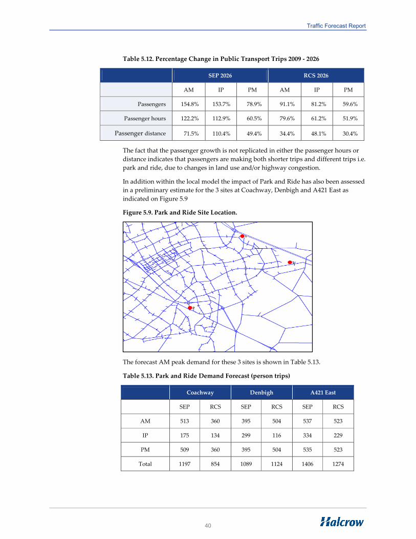
Table 5.12 shows the relative increase in public transport trips as a percentage change

from 2009.


40

Table 5.12. Percentage Change in Public Transport Trips 2009 - 2026

SEP 2026 RCS 2026

AM IP PM AM IP PM

Passengers 154.8% 153.7% 78.9% 91.1% 81.2% 59.6%

Passenger hours 122.2% 112.9% 60.5% 79.6% 61.2% 51.9%

Passenger distance 71.5% 110.4% 49.4% 34.4% 48.1% 30.4%

The fact that the passenger growth is not replicated in either the passenger hours or

distance indicates that passengers are making both shorter trips and different trips i.e.

park and ride, due to changes in land use and/or highway congestion.

In addition within the local model the impact of Park and Ride has also been assessed

in a preliminary estimate for the 3 sites at Coachway, Denbigh and A421 East as

indicated on Figure 5.9

Figure 5.9. Park and Ride Site Location.

The forecast AM peak demand for these 3 sites is shown in Table 5.13.

Table 5.13. Park and Ride Demand Forecast (person trips)

Coachway Denbigh A421 East

SEP RCS SEP RCS SEP RCS

AM 513 360 395 504 537 523

IP 175 134 299 116 334 229

PM 509 360 395 504 535 523

Total 1197 854 1089 1124 1406 1274


41

The above table provides a preliminary forecast to gauge potential future demand

which may assist with determining park and ride parking provision. Revisions to

parameters, service provision, fares, and car park charges or network infrastructure

will influence future patronage.

5.6 Congestion hotspots

Analysis of the traffic model outputs has been undertaken to identify those locations

where congestion will have deteriorated beyond an acceptable level. The main

parameter used to identify this concentrating primarily on the MK urban area is

where the ratio of flow to capacity (RFC) is greater than 90% for links and/or

junctions. The figure of 90% has been chosen as this is consistent with the figure

chosen by the Highway’s Agency’s consultants in assessing traffic impact on the

Strategic Road Network as being the level at which severe congestion and unreliable

journey times become present.

Plots of these from the respective highway model are provided for the base year

situation and the two scenarios modelled. These are contained within Appendix B.

Viewing these plots indicates that in 2009 RFC values over 90% were fairly limited

and showed a similar representation between both AM and PM peaks. The inter peak

showed no junctions with such an RFC.

In the 2026 scenarios although it is clear that the number of junctions reaching

capacity has increased there are some, which, due to improvement works assumed

within the network, have decreased values of congestion. Primarily these are located

along the A422 where signalisation of the roundabouts is proposed.

The SEP scenario figures are indicative only as since the RSS revocation revisions to

the Milton Keynes Transport Model have not been carried through to this scenario.

They do, however, provide some indication of worsening conditions had that

quantum of development be taken forward.

The figures in Appendix B3 for the RCS scenario show deteriorating conditions and it

is these locations which require future investigation.

Table 5.14 indicates the number of junctions which experience a RFC of over 90%

between the scenarios and the base year.

Table 5.14. Number of Junctions with RFC >90% (RCS Scenario)

The plots indicate clearly where attention needs to be concentrated to determine the

level of congestion and queuing and whether this would demonstrate real problems

into the future.

AM Peak Inter Peak PM Peak

Base Year 3 0 5

SEP 25 14 33

RCS 14 4 24


42

5.7 Journey Time Impacts

In a similar manner to the comparison cordon and screenline flows undertaken to

determine the forecast impact of traffic growth a comparison has also been made of

the journey time routes surveyed for the base year model development.

In total 8 routes were assessed as shown in Figure 5.10 and summarised in table 5.15.

Figure 5.10 Journey Time Routes

Table 5.15. Journey Time Route Description

Route Name Road

1 A421 to M1 Junction 13 A421

2 Old Stratford to Chicheley A5, A422 & A509

3 Old Stratford to Watling St, Little Brickhill A5

4 Portway/Fulmer St. to Newport Pagnell A509

5 Childs Way/Tattenhoe St. to Moulsoe A4146, Childs Way

6 A4146/Stoke Rd. to Saxon St/Newport Rd

7 M1 Junction 13 - Junction 15 M1

8 Brunel Rndabout, Bletchley to Newport Pagnell A4146


43

Table 5.16.Journey Time Comparison AM Peak 2009 - 2026

Route Direction Name Road AM 2009 (Min)

SEP % change

RCS % change

Eastbound A421 to M1 Junction 13 A421 16.0 43% 33%

1

Westbound A421 to M1 Junction 13 A421 14.9 30% 25%

Eastbound Old Stratford to Chicheley A5, A422 & A509 16.0 20% 22%

2

Westbound Chicheley to Old Stratford A509, A422 & A5 17.4 1% 4%

Southbound Old Stratford to Watling St, Little Brickhill A5 13.8 31% 28%

3

Northbound Watling St., Little Brickhill to Old Stratford A5 15.7 45% 16%

Eastbound Portway/Fulmer St. to Newport Pagnell A509 16.7 44% 49%

4

Westbound Newport Pagnell to Portway/Fulmer St. A509 18.2 28% 43%

Eastbound Childs Way/Tattenhoe St. to Moulsoe A4146, Childs

Way 18.8 32% 32%

5

Westbound Moulsoe to Childs Way/Tattenhoe St. Childs Way,

A4146 18.9 21% 35%

Northbound A4146/Stoke Rd. to Saxon St/Newport Rd 19.6 38% 31%

6

Southbound Saxon St/Newport Rd to A4146/Stoke Rd 18.9 15% 15%

Northbound M1 Junction 13 - Junction 15 M1 16.0 30% 7%

7

Southbound M1 Junction 15 - Junction 13 M1 12.9 63% 47%

Northbound Brunel Rndabout, Bletchley to Newport Pagnell A4146 17.0 30% 29%

8

Southbound Newport Pagnell to Brunel Rndabout, Bletchley A4146 17.5 32% 34%


44

Table 5.17.Journey Time Comparison Inter Peak 2009 - 2026

Route Direction Name Road IP

2009

SEP

% change

RCS

% change

Eastbound A421 to M1 Junction 13 A421 14.0 38% 30% 1


Eastbound Old Stratford to Chicheley A5, A422 & A509 13.0 22% 21% 2


Southbound Old Stratford to Watling St, Little Brickhill A5 12.2 21% 16% 3


Eastbound Portway/Fulmer St. to Newport Pagnell A509 15.4 19% 16% 4


Eastbound Childs Way/Tattenhoe St. to Moulsoe A4146, Childs Way 16.1 12% 10% 5

Westbound Moulsoe to Childs Way/Tattenhoe St. Childs Way, A4146 15.7 21% 17%

Northbound A4146/Stoke Rd. to Saxon St/Newport Rd 17.5 19% 14% 6


Northbound M1 Junction 13 - Junction 15 M1 16.0 23% 4% 7


Northbound Brunel Rndabout, Bletchley to Newport Pagnell A4146 15.6 23% 17% 8



45

Table 5.18.Journey Time Comparison PM Peak 2009 - 2026

Route Direction Name Road PM

2009

(mins)

SEP

% change

RCS

% change

Eastbound A421 to M1 Junction 13 A421 15.5 24% 19% 1


Eastbound Old Stratford to Chicheley A5, A422 & A509 18.5 9% 9% 2


Southbound Old Stratford to Watling St, Little Brickhill A5 14.8 19% 15% 3


Eastbound Portway/Fulmer St. to Newport Pagnell A509 18.0 36% 38% 4


Eastbound Childs Way/Tattenhoe St. to Moulsoe A4146, Childs Way 19.1 7% 5% 5

Westbound Moulsoe to Childs Way/Tattenhoe St. Childs Way, A4146 17.2 38% 32%

Northbound A4146/Stoke Rd. to Saxon St/Newport Rd 18.4 34% 33% 6


Northbound M1 Junction 13 - Junction 15 M1 16.7 29% 8% 7


Northbound Brunel Rndabout, Bletchley to Newport Pagnell A4146 16.9 44% 41% 8



46

Analysis of the journey time increases shows that for the RCS scenario percentage

increases in time are of the order of upto a maximum of 49% on a journey time of 16

minutes. In the inter peak period increase are in the region of 20% whilst in the PM

peak increase are up to 44% (A5 Northbound)

Over all journey time routes the modelled forecast times indicate that on average AM

peak journey times increase by 4.7 minutes, Inter peak times by 2.2 minutes and PM

peak times by 3.7 minutes compared to the average times in 2009.

5.8 Strategic Road Network Impact

Due to the proximity of strategic road network links in the form of the M1 and A5 a

comparison of traffic growth for the RCS scenario has been undertaken. This has

focused on outputs from the highway model and has considered the change in flow

(in pcus) and the RFC value as output by the SATURN model.

M1

The section of the M1 which is included within the detailed model area (junctions 12 -

15) has been examined. Tables 5.19 to 5.22 show the respective traffic flows as actual

flows in pcus.

Table 5.19. M1 AM Peak Southbound

Year/Scenario J15 -J14 J14 - J13 J13 - J12

2009 Base Year 4862 4144 4260

2026 RCS 5802 5101 5786

2009 - 2026 19% 23% 36%

Table 5.20 M1 AM Peak Northbound


2009 Base Year 3712 4488 4550

2026 RCS 4426 5475 5401

2009 - 2026 19% 22% 19%

Table 5.21 M1 PM Peak Southbound


2009 Base Year 4111 4595 4603

2026 RCS 4790 5412 5801

2009 - 2026 17% 18% 26%

Table 5.22 M1 PM Peak Northbound


2009 Base Year 4667 4559 4761

2026 RCS 5322 5162 5601

2009 - 2026 14% 13% 18%


47

The above tables indicate that due to the forecast growth in traffic from general

regional growth and that pertaining to the Milton Keynes Core Strategy that flows on

the M1 are due to rise. This varies by direction and peak hour with maximum flows

reaching approximately 5800 pcus on J12-J13 and J14 – J15 with percentage increase

ranging from 13% to 36%.

M1 Volume/Capacity ratios

Increase in traffic flow can lead to increases in congestion, flow breakdown and

stress. Stress can be assessed in terms of the ratio of flow to capacity as indicated

earlier (with reference to the SATURN plots in Appendix B). Following information

from the Highways Agency RFC’s have been grouped into four key categories to

reflect the level of congestion and reliability of journey times as indicated below.

Table 5.23. Network Stress defined bandings.

Tables 5.24 – 5.27 show the comparison of RFC for those relevant sections of the M1.

Table 5.24. M1 Am Peak Southbound RFC


2009 Base Year 77 66 64

2026 RCS 92 81 66

2009 - 2026 19% 23% 3%

Table 5.25. M1 Am Peak Northbound RFC


2009 Base Year 56 68 72

2026 RCS 70 83 62

2009 - 2026 25% 22% -14%

Table 5.26. M1 PM Peak Southbound RFC


2009 Base Year 65 73 69

2026 RCS 76 86 66

2009 - 2026 17% 18% -4%

Table 5.27. M1 PM Peak Northbound RFC


2009 Base Year 71 69 76

2026 RCS 80 78 64

2009 - 2026 13% 13% -16%


48

The above comparison indicates that only one link will experience a level of stress

likely to cause severe congestion in 2026, this being J15 to J14 in the AM peak. Other

sections, mainly J14 – J13 experience moderate stress. The results for J13 – J12 show a

reduction in stress in both directions in the PM peak and northbound in the AM peak.

This is reflective of the increased capacity this section has as a result of the M1 J10 –

J13 improvement incorporating hard should running which opened after the base

year model had been completed but is incorporated in the forecast year models.

A5

A similar comparison has been undertaken for the A5 sections within Milton Keynes

shown in table 5.28 to 5.31.

Table 5.28. A5 Southbound AM Peak, Actual flows

Year/Scenario Bletcham Way

to Little

Brickhill

A421 to

Bletcham

Way

A509 to

A421

A422 to

A509

A508 to

A422

2009 Base Year 1176 1482 2028 3302 3014

2026 RCS 1431 2308 2923 4227 3292

2009 - 2026 22% 56% 44% 28% 9%

Table 5.29 A5 Northbound AM Peak, Actual flows


to Little

Brickhill

A421 to

Bletcham

Way

A509 to

A421

A422 to

A509

A508 to

A422

2009 Base Year 1870 2102 2373 1895 1206

2026 RCS 1911 2688 3327 2530 1577

2009 - 2026 2% 28% 40% 34% 31%

Table 5.30 A5 Southbound PM Peak, Actual flows


to Little

Brickhill

A421 to

Bletcham

Way

A509 to

A421

A422 to

A509

A508 to

A422

2009 Base Year 1405 1917 1846 1638 1327

2026 RCS 2122 2756 2730 2353 1728

2009 - 2026 51% 44% 48% 44% 30%

Table 5.31 A5 Northbound AM Peak, Actual flows


to Little

Brickhill

A421 to

Bletcham

Way

A509 to

A421

A422 to

A509

A508 to

A422

2009 Base Year 1399 1940 2772 3532 2689

2026 RCS 1758 2624 3427 3839 2784

2009 - 2026 26% 35% 24% 9% 4%


49

Tables 5.32 to 5.35 show the respective RFC performance for each of the links based

on the congestion level banding proposed in table 5.23.

Table 5.32. A5 Southbound AM Peak, RFC


to Little

Brickhill

A421 to

Bletcham

Way

A509 to

A421

A422 to

A509

A508 to

A422

2009 Base Year 101 36 48 76 71

2026 RCS 39 54 69 99 77

2009 - 2026 -61% 50% 44% 30% 8%

Table 5.33 A5 Northbound AM Peak, RFC


to Little

Brickhill

A421 to

Bletcham

Way

A509 to

A421

A422 to

A509

A508 to

A422

2009 Base Year 44 50 56 45 28

2026 RCS 45 63 79 60 37

2009 - 2026 2% 26% 41% 33% 32%

Table 5.34 A5 Southbound PM Peak, RFC


to Little

Brickhill

A421 to

Bletcham

Way

A509 to

A421

A422 to

A509

A508 to

A422

2009 Base Year 107 45 43 39 31

2026 RCS 84 65 64 55 41

2009 - 2026 -21% 44% 49% 41% 32%

Table 5.35 A5 Northbound PM Peak, RFC


to Little

Brickhill

A421 to

Bletcham

Way

A509 to

A421

A422 to

A509

A508 to

A422

2009 Base Year 33 46 65 83 63

2026 RCS 41 62 81 90 65

2009 - 2026 24% 35% 25% 8% 3%

Performance on the A5 is varied with improvements seen as a result of the

signalisation of the A5/A4146 roundabout at Little Brickhill reducing link based stress

levels during a period when traffic volumes have grown.

The largest growth in traffic tends to be on the sections between the A421 and A422

which would represent a greater propensity for junction hoping between areas in

Milton Keynes as well as dealing with overall traffic growth.


50

The section between the A422 and A509 northbound in both peaks shows signs of

increased stress and potential severe congestion and should be investigated further.


51

6 Conclusion

Halcrow, in association with RAND Europe, Stirling Maynard Transportation (SMT)

and Count on Us were appointed by Milton Keynes Council (MKC )in 2009 to

develop an up to date transport modelling capability for the Milton Keynes (MK)

area. This involved the development of spatially detailed highway and pubic

transport models and their interaction to demand models to enable the assessment of

planning and infrastructure schemes planned for the Milton Keynes area.

The model is a behaviourally based four stage model developed in line with current

WebTAG guidance on model form and procedures. The model determines the travel

demand from the underlying characteristics of the transport supply and the

characteristics of the travellers in the area.

The demand models take population and employment data as an input and use trip

rates to generate the travel demand across all modes of travel to all destinations

based on the respective change in cost of travel by the different modes. A demand

model is required as a result of major changes in travel demand expected in and

around Milton Keynes as a result of major land use and infrastructure changes over

the next twenty years or so.

The base year 2009 Milton Keynes Transport Model has been approved by the

Highways Agency as providing a robust representation of base year traffic flows

based on the strategic and local highway network. As a result it has been confirmed

as providing a suitable platform for the development of a 2026 forecast model capable

of assessing the proposed Core Strategy for development and infrastructure in Milton

Keynes to 2026.

The 2026 Forecast models took planning and infrastructure information for 2

scenarios, one based on the revocated South East Plan (SEP) and the other, a Revised

Core Strategy for Milton Keynes. Due to changes to the Milton Keynes Transport

Model since initial forecasts and the fact that the SEP is no longer valid the majority

of results in this report have concentrated on the RCS strategy.

Planning data for the RCS provided indicated a desire for an additional 27,608

households (as opposed to 44,457 for the SEP) to be built within the MK area in the

period to 2026, combined with an intention of creating 1.5 jobs per household (an

additional 41,412 jobs) this represented a significant increase in travel demand.

Infrastructure schemes for both highway and public transport networks for both the

strategic and local networks were compiled and updated within the respective model

platforms. Planning inputs were applied to both the Regional and Local demand

models.

The resultant highway trip growth for the RCS scenario increased vehicle trips by

20% in the AM and PM peaks and 32% in the inter peak period. This level of growth

led to increased total travel times of up to 50% and travel distance of between 19%

and 25%. Whilst travelling conditions have deteriorated within the MKC area the

network still operates to a suitable level.

Allied to the highway trip growth has been a significant percentage increase in public

transport trips of up to 90% in the AM peak (albeit from a low base year total). Public

transport travel times and distances have not increased by a similar level indicating


52

an increase in shorter distance trips due both to increased congestion, improved

public transport provision and the implementation of park and ride initiatives.

Analysis of traffic flows and stress levels on the strategic road network links of the

M1 and A5 within and adjacent to Milton Keynes has also established that whilst

traffic growth occurs severe congestion is not predicted on the network as a whole.

Increase in flows on A5 sections indicates an increased level of junction hopping

which does create congestion particularly for the A422 to A509 section.

Plots of congestion and increased levels of highway stress have been provided

primarily to identify locations for further investigation as so far with the modelling

undertaken neither mitigation works have been undertaken to ascertain whether the

congestion indicated could be ameliorated nor whether it is specific to any particular

development. This is a particular area where attention should now be directed.


Appendix A Planning Data


A.1 MKC Planning Data: SEP and RCS Scenarios



Appendix B SATURN Model Plots

.


B.1 2009 Base Year Model: Nodes/Links RFC > 0.90

2009 AM Peak

2009 Inter Peak


2009 PM Peak


B.2 2026 SEP Scenario: Nodes/Links RFC > 0.90

2026 SEP AM Peak

2026 SEP Inter Peak


2026 SEP PM Peak


B.3 2026 RCS Scenario: Nodes/Links RFC > 0.90

2026 RCS AM Peak

2026 RCS Inter Peak


2026 RCS PM Peak

For details of your nearest Halcrow office, visit our website halcrow.com

Documents

Milton Keynes Transport Model Traffic Forecast Report