Midterm Review

Calculus

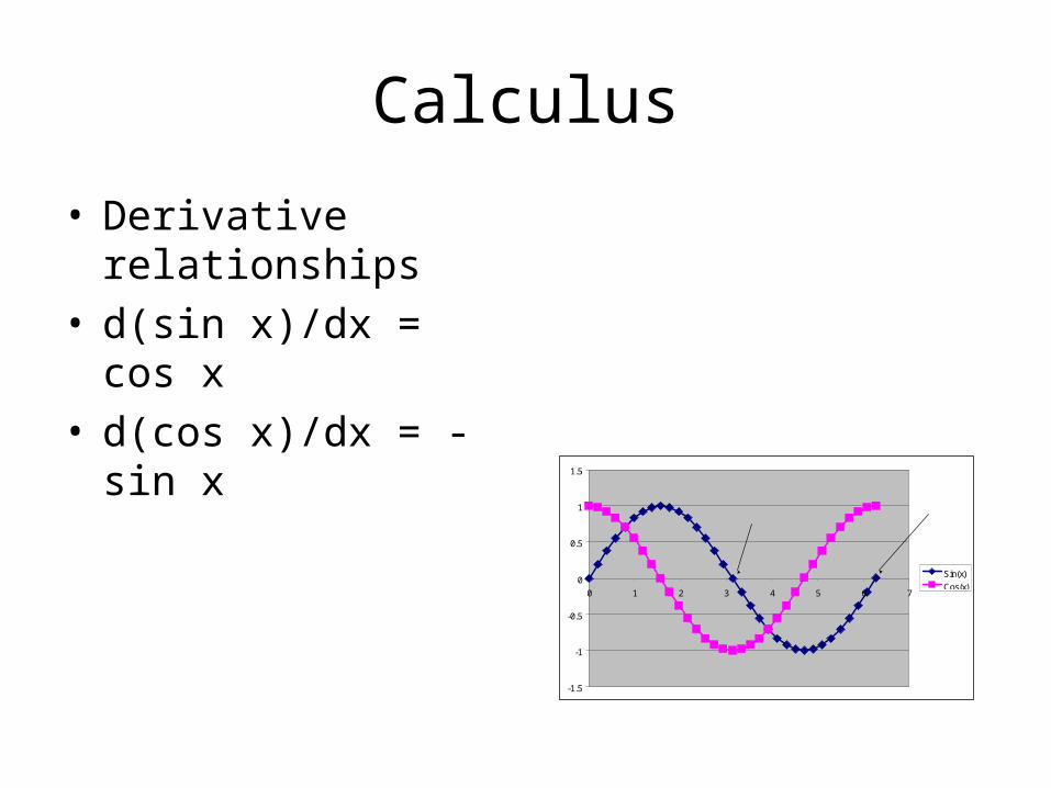
• Derivative relationships

• d(sin x)/dx = cos x• d(cos x)/dx = -sin x

-1.5

-1

-0.5

0

0.5

1

1.5

0 1 2 3 4 5 6 7

Sin(x)

Cos(x)

Calculus

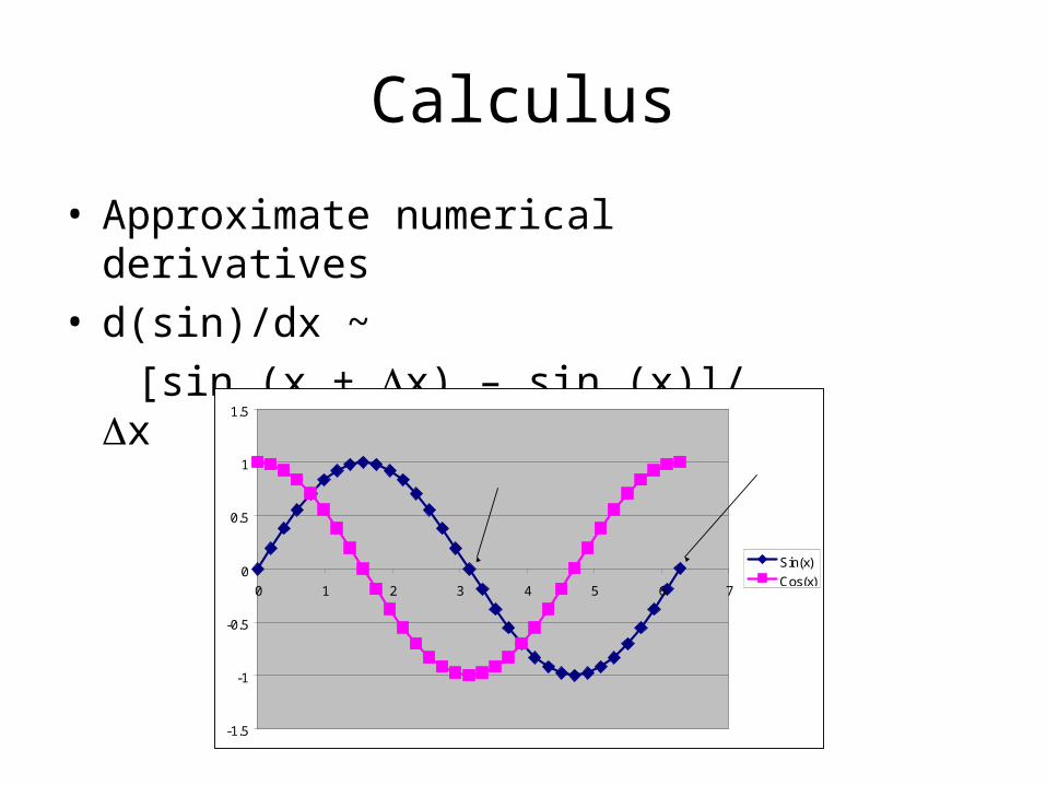
• Approximate numerical derivatives• d(sin)/dx ~

[sin (x + x) – sin (x)]/ x

-1.5

-1

-0.5

0

0.5

1

1.5

0 1 2 3 4 5 6 7

Sin(x)

Cos(x)

Calculus

• Partial derivatives• h(x,y) = x4 + y3 + xy• The partial derivative of h with respect to x

at a y location y0 (i.e., ∂h/∂x|y=y0),

• Treat any terms containing y only as constants – If these constants stand alone they drop out of

the result – If the constants are in multiplicative terms

involving x, they are retained as constants

• Thus ∂h/ ∂x|y=y0 = 4x3 + y0

Ground Water Basics

• Porosity

• Head

• Hydraulic Conductivity

• Transmissivity

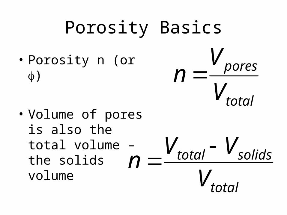
Porosity Basics

• Porosity n (or )

• Volume of pores is also the total volume – the solids volume

total

pores

V

Vn

total

solidstotal

V

VVn

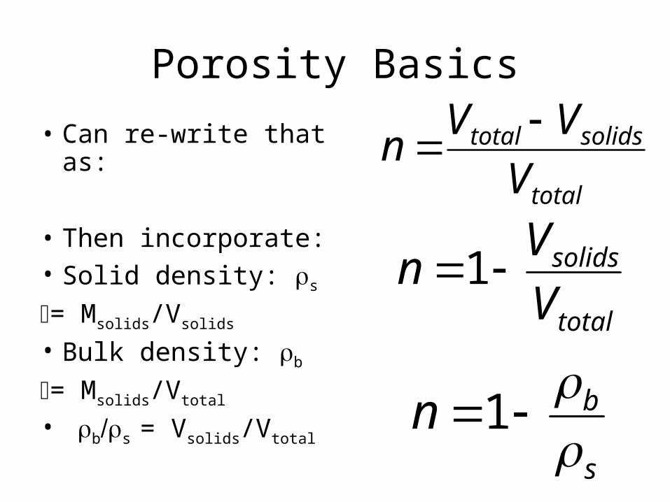
Porosity Basics

• Can re-write that as:

• Then incorporate:• Solid density: s

= Msolids/Vsolids

• Bulk density: b

= Msolids/Vtotal • bs = Vsolids/Vtotal

total

solidstotal

V

VVn

total

solids

V

Vn 1

s

bn

1

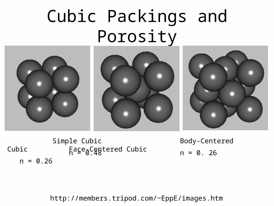
Cubic Packings and Porosity

http://members.tripod.com/~EppE/images.htm

Simple Cubic Body-Centered Cubic Face-Centered Cubic n = 0.48 n = 0. 26 n = 0.26

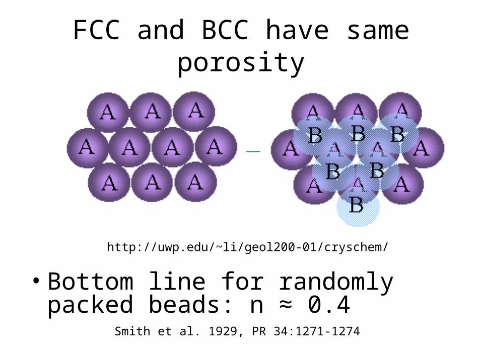
FCC and BCC have same porosity

• Bottom line for randomly packed beads: n ≈ 0.4

                                                             

http://uwp.edu/~li/geol200-01/cryschem/

Smith et al. 1929, PR 34:1271-1274

Effective

Porosity

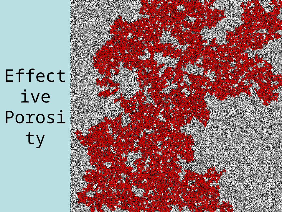
Effective

Porosity

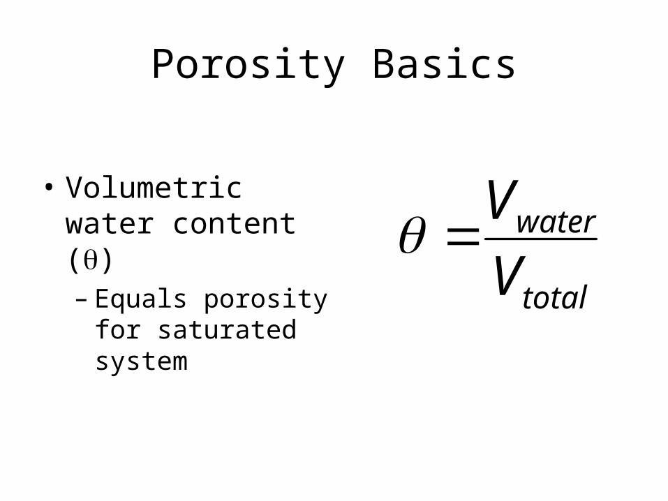
Porosity Basics

• Volumetric water content ()– Equals porosity for

saturated system total

water

V

V

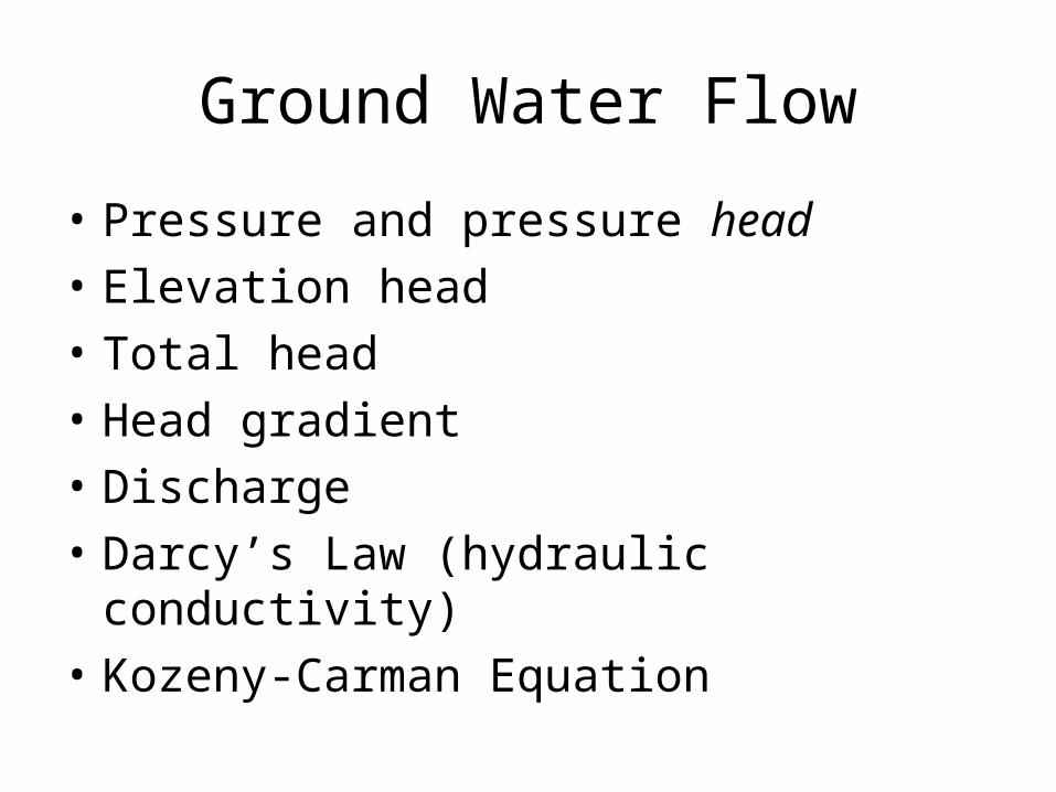
Ground Water Flow

• Pressure and pressure head

• Elevation head

• Total head

• Head gradient

• Discharge

• Darcy’s Law (hydraulic conductivity)

• Kozeny-Carman Equation

Multiple Choice:Water flows…?

• Uphill

• Downhill

• Something else

Pressure

• Pressure is force per unit area• Newton: F = ma

– Fforce (‘Newtons’ N or kg m s-2)– m mass (kg)– a acceleration (m s-2)

• P = F/Area (Nm-2 or kg m s-2m-2 =

kg s-2m-1 = Pa)

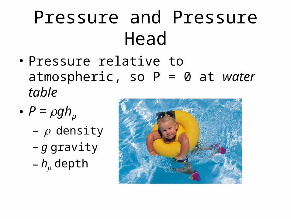
Pressure and Pressure Head

• Pressure relative to atmospheric, so P = 0 at water table

• P = ghp

– density– g gravity

– hp depth

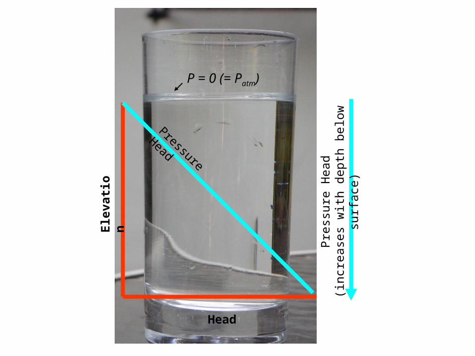
P = 0 (= Patm)

Pre

ssur

e H

ead

(incr

ease

s w

ith d

epth

bel

ow s

urfa

ce)

Pressure Head

Elevation

Head

Elevation Head

• Water wants to fall

• Potential energy

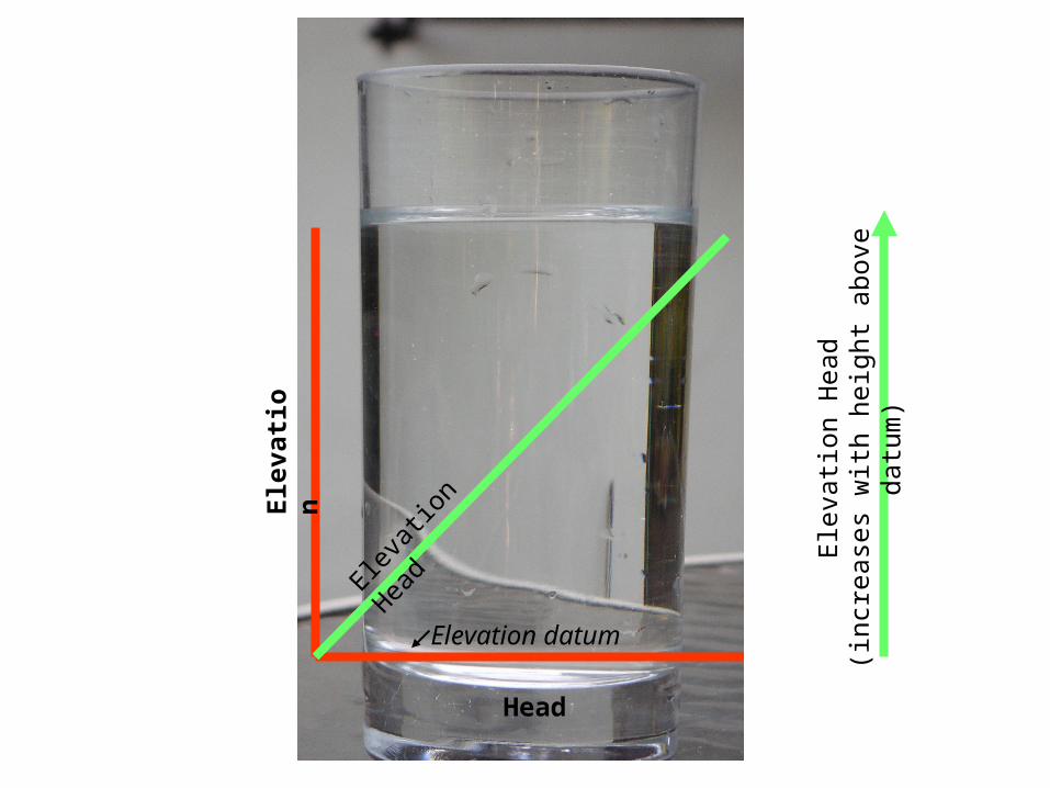
Ele

vatio

n H

ead

(incr

ease

s w

ith h

eigh

t ab

ove

datu

m)

Eleva

tion

Head

Elevation

Head

Elevation datum

Total Head

• For our purposes:

• Total head = Pressure head + Elevation head

• Water flows down a total head gradient

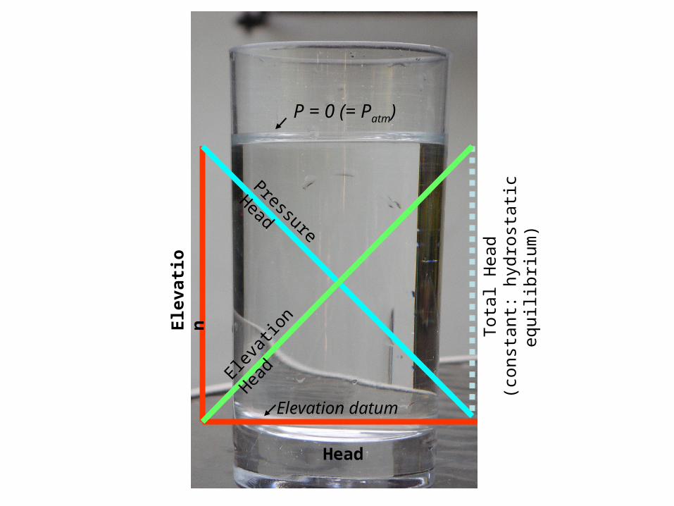
P = 0 (= Patm)

Tot

al H

ead

(con

stan

t: h

ydro

stat

ic e

quili

briu

m)

Pressure Head

Eleva

tion

Head

Elevation

Head

Elevation datum

Head Gradient

• Change in head divided by distance in porous medium over which head change occurs

• dh/dx [unitless]

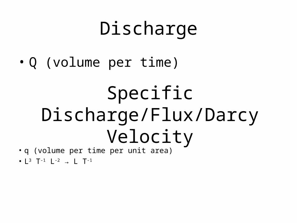
Discharge

• Q (volume per time)

Specific Discharge/Flux/Darcy Velocity

• q (volume per time per unit area)• L3 T-1 L-2 → L T-1

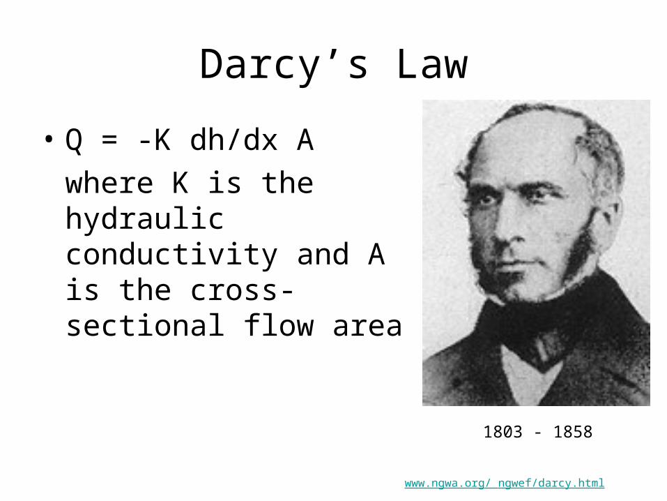
Darcy’s Law

• Q = -K dh/dx A

where K is the hydraulic conductivity and A is the cross-sectional flow area

www.ngwa.org/ ngwef/darcy.html

1803 - 1858

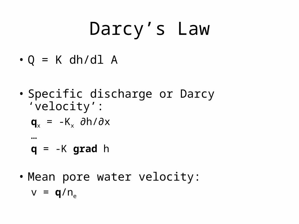
Darcy’s Law

• Q = K dh/dl A

• Specific discharge or Darcy ‘velocity’:qx = -Kx ∂h/∂x…q = -K grad h

• Mean pore water velocity:v = q/ne

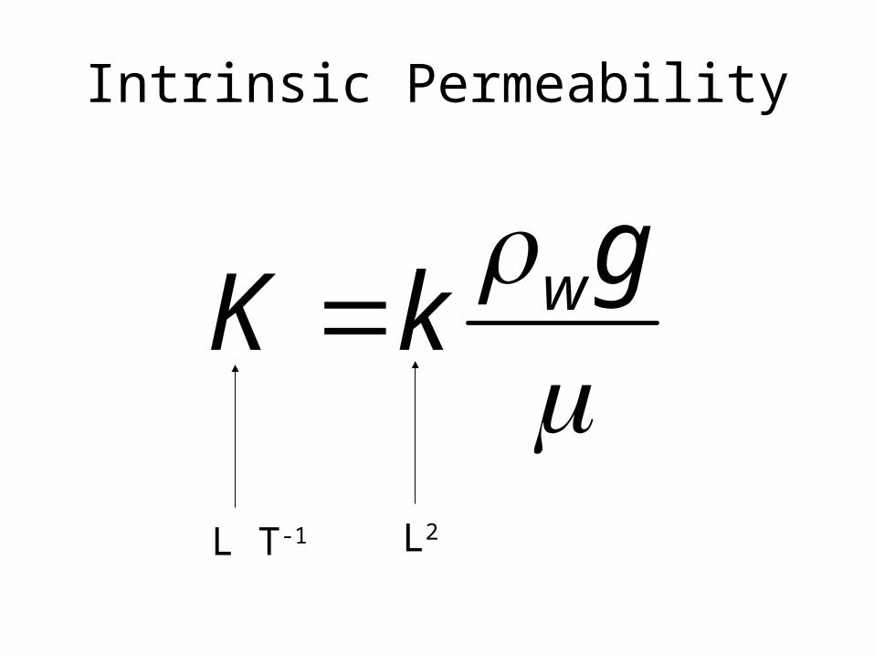
Intrinsic Permeability

gkK w

L T-1 L2

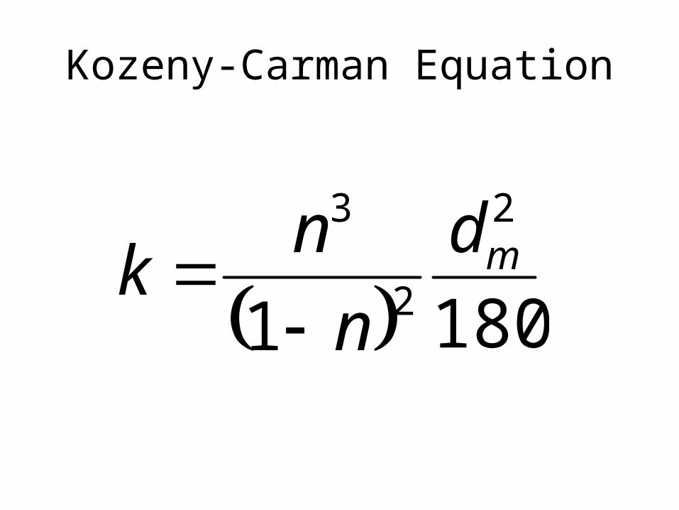
Kozeny-Carman Equation

1801

2

2

3md

n

nk

Transmissivity

• T = Kb

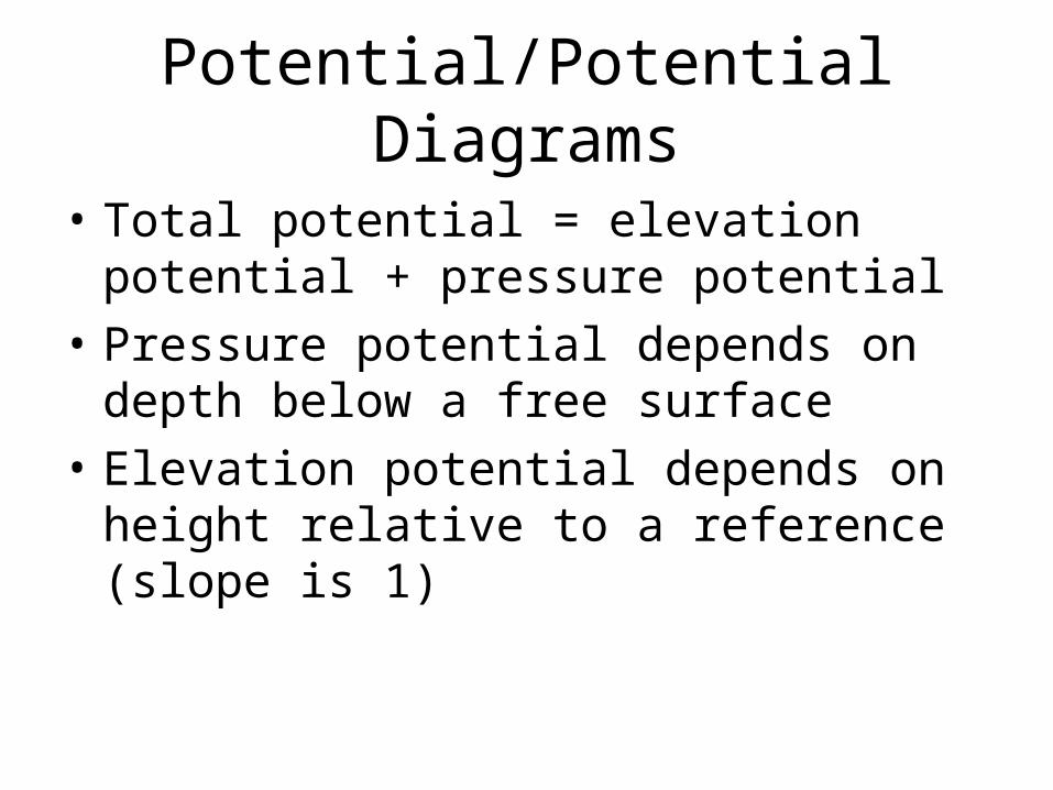
Potential/Potential Diagrams

• Total potential = elevation potential + pressure potential

• Pressure potential depends on depth below a free surface

• Elevation potential depends on height relative to a reference (slope is 1)

Darcy’s Law

• Q = -K dh/dl A

• Q, q

• K, T

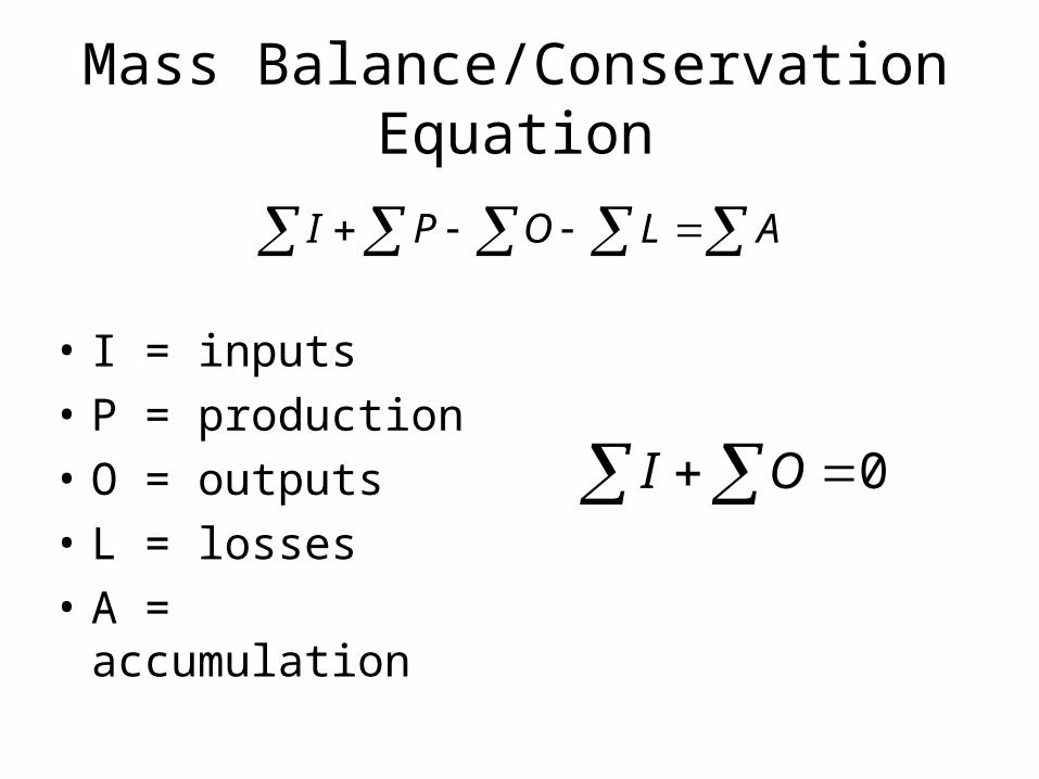
Mass Balance/Conservation Equation

• I = inputs

• P = production

• O = outputs

• L = losses

• A = accumulation

ALOPI

0OI

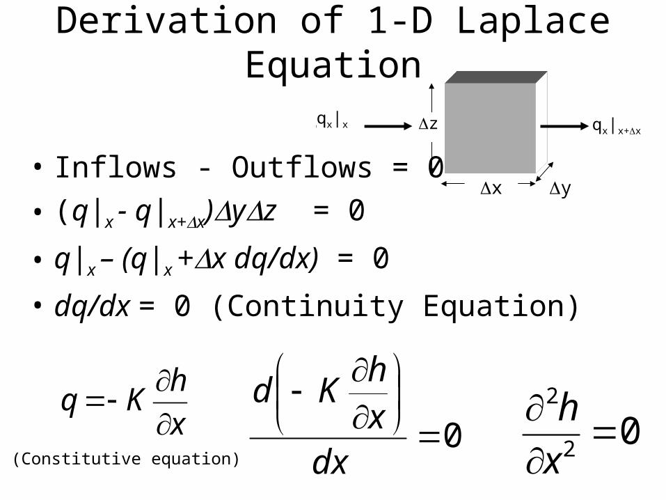
Derivation of 1-D Laplace Equation

• Inflows - Outflows = 0

• (q|x - q|x+x)yz = 0

• q|x – (q|x +x dq/dx) = 0

• dq/dx = 0 (Continuity Equation)

x

hKq

x y

qx|x qx|x+xz

0

dxxh

Kd0

2

2

x

h(Constitutive equation)

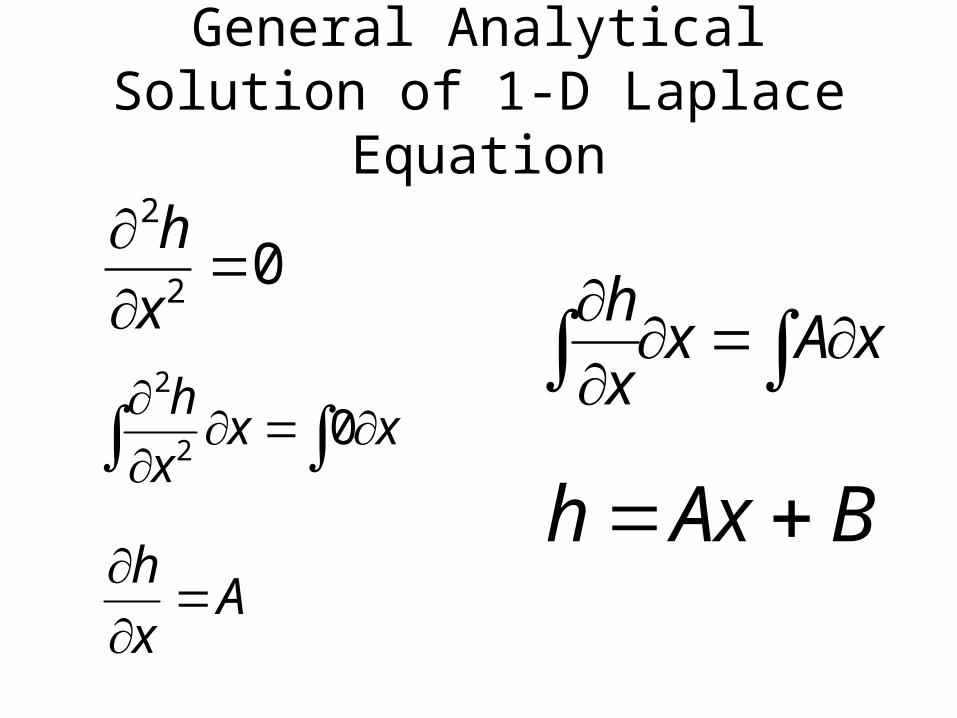
General Analytical Solution of 1-D Laplace Equation

Ax

h

xAxx

h

0

2

2

x

h

xxx

h0

2

2

BAxh

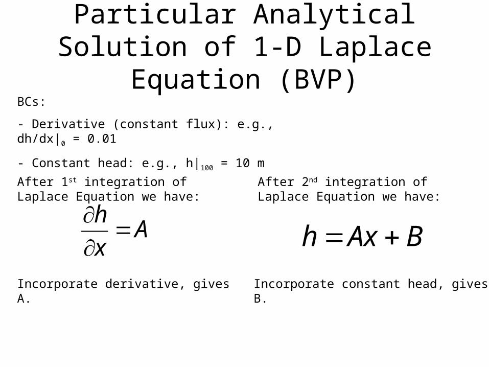
Particular Analytical Solution of 1-D Laplace Equation (BVP)

Ax

h

BAxh

BCs:

- Derivative (constant flux): e.g., dh/dx|0 = 0.01

- Constant head: e.g., h|100 = 10 m

After 1st integration of Laplace Equation we have:

Incorporate derivative, gives A.

After 2nd integration of Laplace Equation we have:

Incorporate constant head, gives B.

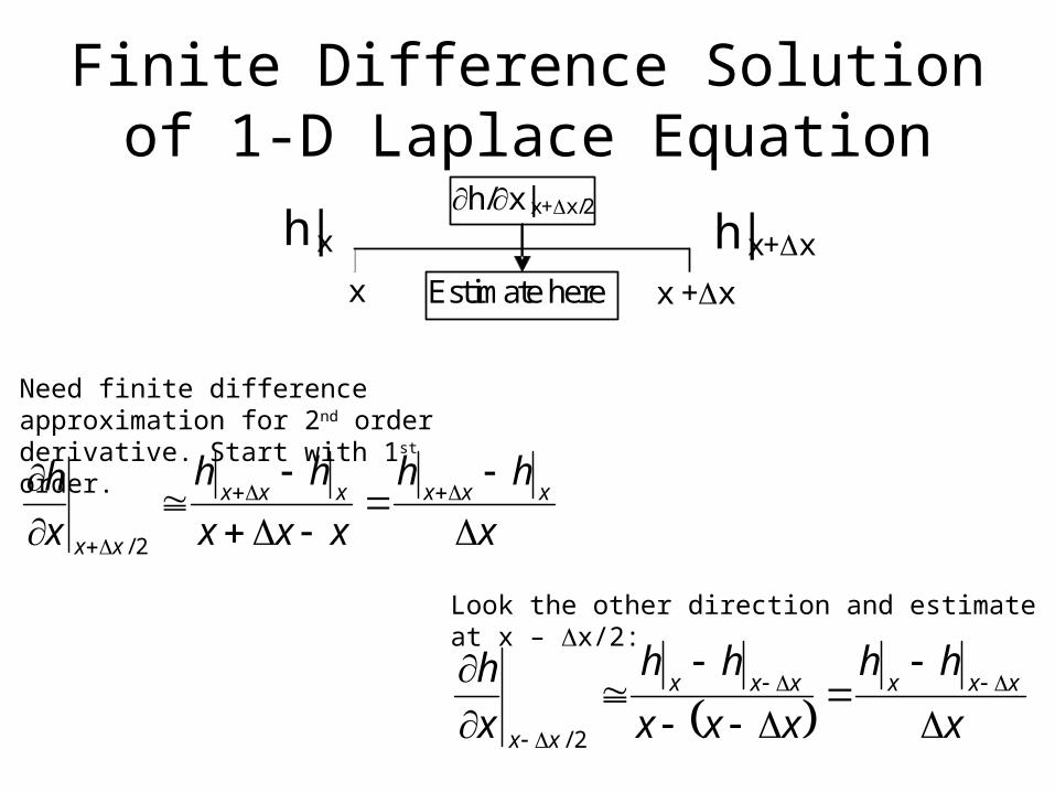
Finite Difference Solution of 1-D Laplace Equation

Need finite difference approximation for 2nd order derivative. Start with 1st order.

Look the other direction and estimate at x – x/2:

x

hh

xxx

hh

x

h xxxxxx

xx

2/

x

hh

xxx

hh

x

h xxxxxx

xx

2/

h|x h|x+x

x x +x

h/x|x+x/2

Estimate here

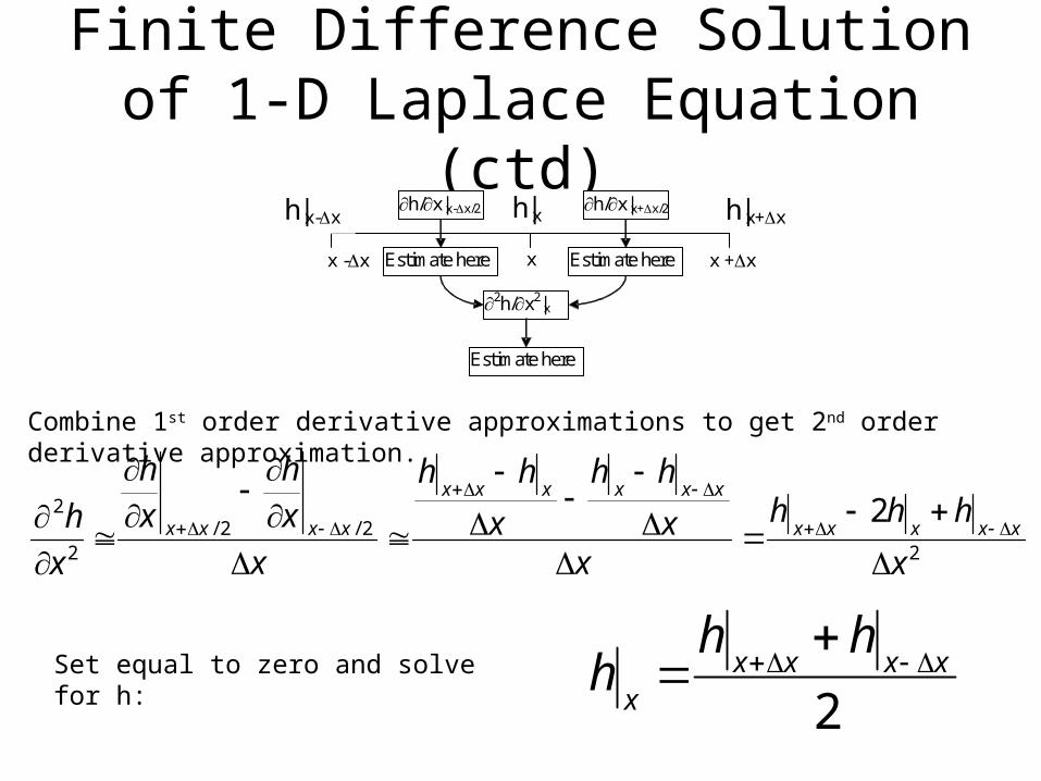
Finite Difference Solution of 1-D Laplace Equation (ctd)

Combine 1st order derivative approximations to get 2nd order derivative approximation.

h|x h|x+x

x x +x

h|x-x

x -x

h/x|x+x/2

Estimate here

h/x|x-x/2

Estimate here

2h/x2|x

Estimate here

22/2/

2

2 2

x

hhh

xx

hh

x

hh

x

x

h

x

h

x

h xxxxx

xxxxxx

xxxx

Set equal to zero and solve for h:

2xxxx

x

hhh

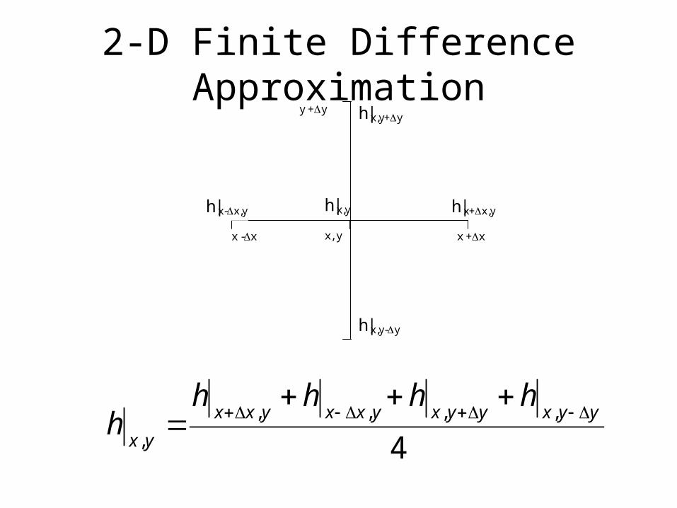
2-D Finite Difference Approximation

h|x,y h|x+x,y

x, y

y +y

h|x-x,y

x -x x +x

h|x,y-y

h|x,y+y

4,,,,

,

yyxyyxyxxyxx

yx

hhhhh

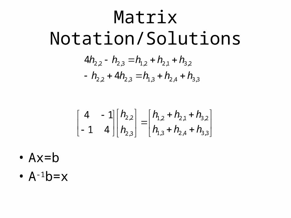
Matrix Notation/Solutions

• Ax=b

• A-1b=x

3,34,23,13,22,2

2,31,22,13,22,2

4

4

hhhhh

hhhhh

3,34,23,1

2,31,22,1

3,2

2,2

41

14

hhh

hhh

h

h

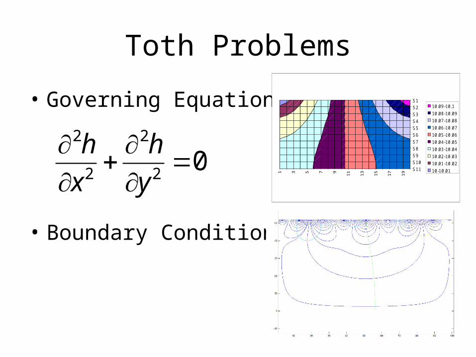
Toth Problems

• Governing Equation

• Boundary Conditions

1 3 5 7 9

11

13

15

17

19

S 1

S 2

S 3

S 4

S 5

S 6

S 7

S 8

S 9

S 10

S 11

10.09-10.1

10.08-10.09

10.07-10.08

10.06-10.07

10.05-10.06

10.04-10.05

10.03-10.04

10.02-10.03

10.01-10.02

10-10.0102

2

2

2

y

h

x

h

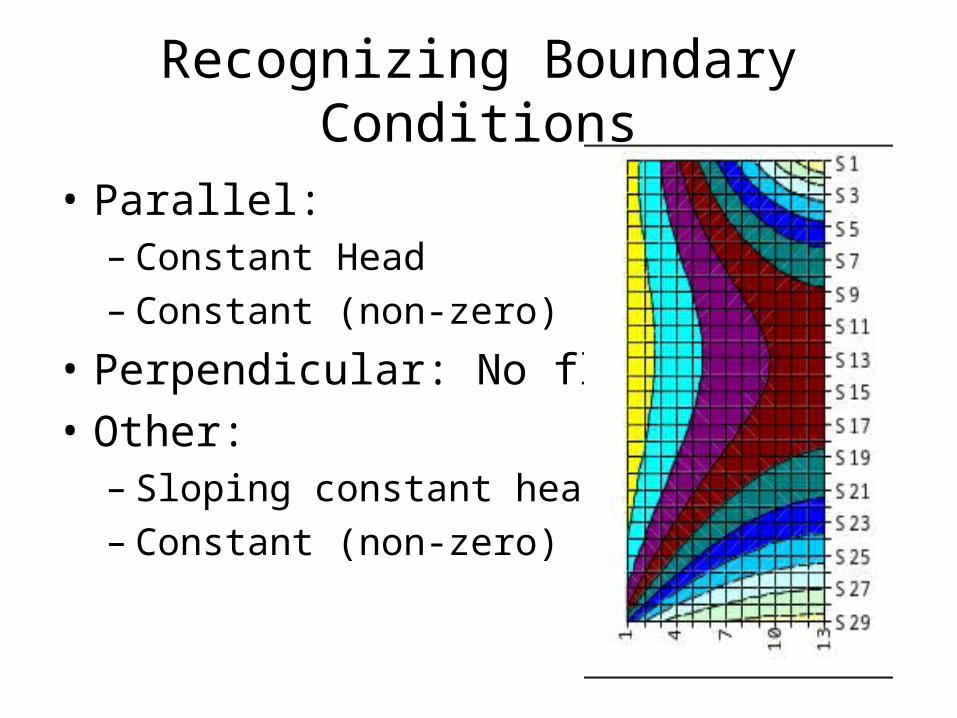
Recognizing Boundary Conditions

• Parallel: – Constant Head – Constant (non-zero) Flux

• Perpendicular: No flow

• Other: – Sloping constant head– Constant (non-zero) Flux

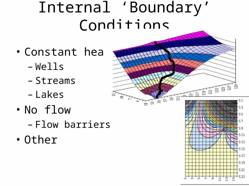
Internal ‘Boundary’ Conditions

• Constant head – Wells– Streams– Lakes

• No flow– Flow barriers

• Other

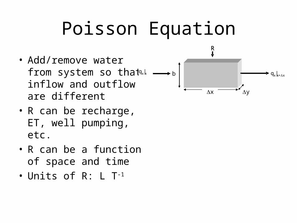
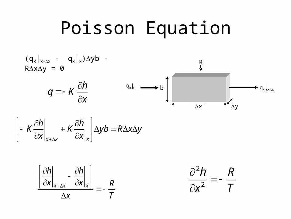
Poisson Equation

• Add/remove water from system so that inflow and outflow are different

• R can be recharge, ET, well pumping, etc.

• R can be a function of space and time

• Units of R: L T-1

x y

qx|x qx|x+xb

R

x y

qx|x qx|x+x

x yx yx y

qx|x qx|x+xb

R

Poisson Equation

x y

qx|x qx|x+xb

R

x y

qx|x qx|x+x

x yx yx y

qx|x qx|x+xb

R(qx|x+x - qx|x)yb -Rxy = 0

x

hKq

yxRybx

hK

x

hK

xxx

T

R

x

xh

xh

xxx

T

R

x

h

2

2

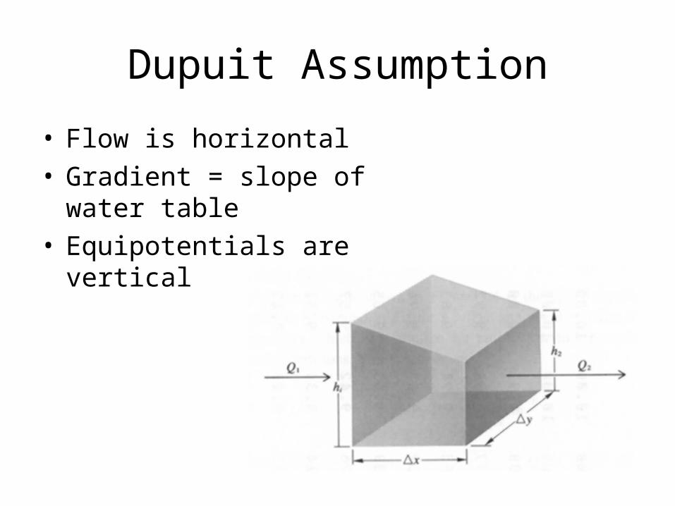
Dupuit Assumption

• Flow is horizontal• Gradient = slope of water table• Equipotentials are vertical

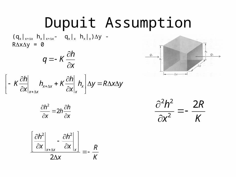
Dupuit Assumption

K

R

x

h 22

22

(qx|x+x hx|x+x- qx|x hx|x)y - Rxy = 0

x

hKq

yxRyhx

hKh

x

hK x

xxx

xx

K

R

x

xh

xh

xxx

2

22

x

hh

x

h

22

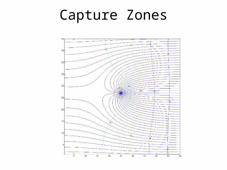
Capture Zones

Water Balance and Model Types

X

0

2x1x

2y

1y

0

Y

Effective outflow boundary

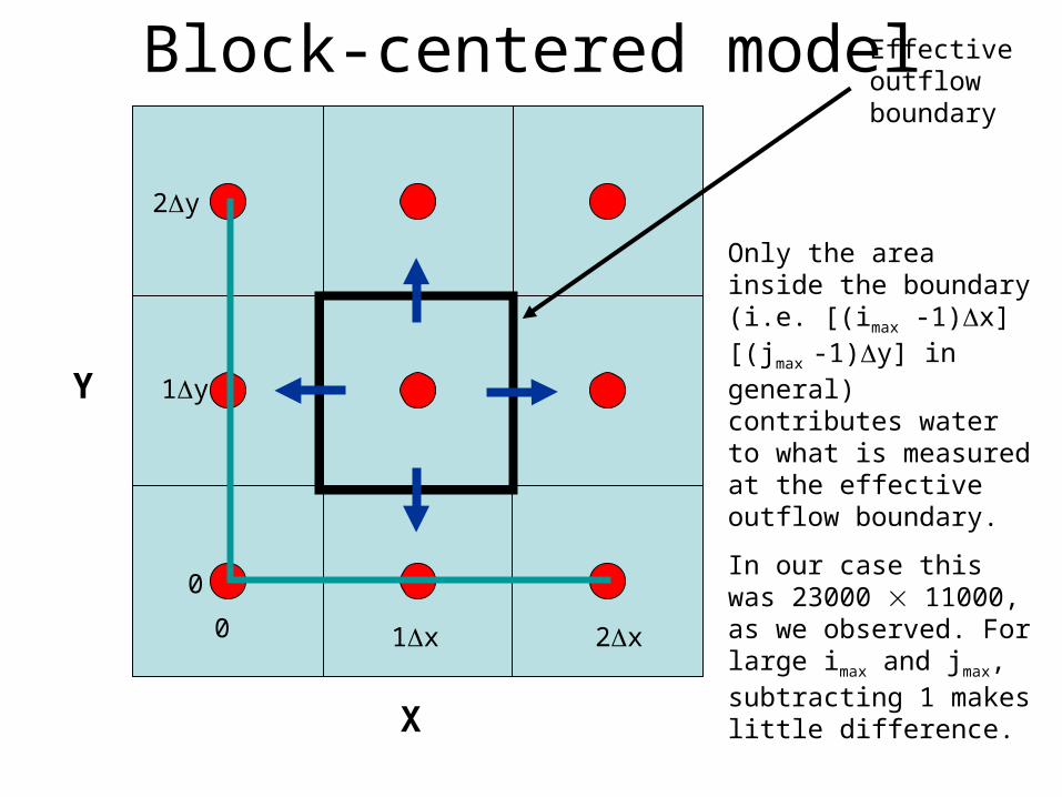
Only the area inside the boundary (i.e. [(imax -1)x] [(jmax -1)y] in general) contributes water to what is measured at the effective outflow boundary.

In our case this was 23000 11000, as we observed. For large imax and jmax, subtracting 1 makes little difference.

Block-centered model

X

0

2x1x

2y

1y

0

Y

Effective outflow boundary

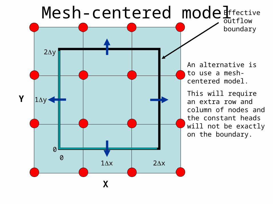
An alternative is to use a mesh-centered model.

This will require an extra row and column of nodes and the constant heads will not be exactly on the boundary.

Mesh-centered model

Summary

• In summary, there are two possibilities:– Block-centered and– Mesh-centered.

• Block-centered makes good sense for constant head boundaries because they fall right on the nodes, but the water balance will miss part of the domain.

• Mesh-centered seems right for constant flux boundaries and gives a more intuitive water balance, but requires an extra row and column of nodes.

• The difference between these models becomes negligible as the number of nodes becomes large.

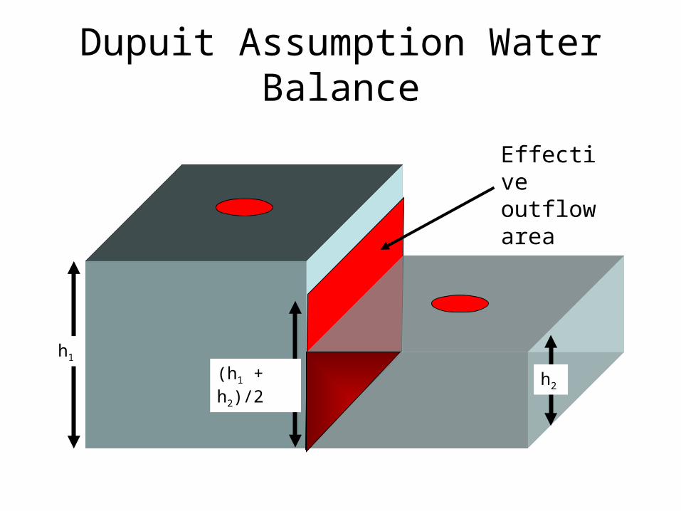
Dupuit Assumption Water Balance

h1

h2

Effective outflow area

(h1 + h2)/2

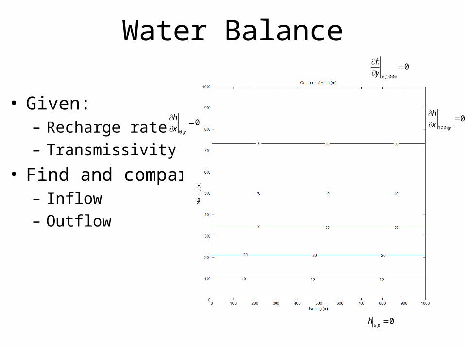
Water Balance

• Given: – Recharge rate – Transmissivity

• Find and compare:– Inflow– Outflow

0,1000

yx

h0

,0

yx

h

01000,

xy

h

00,

xh

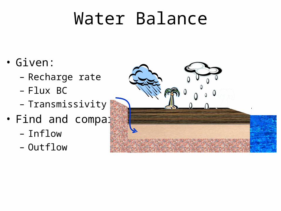
Water Balance

• Given: – Recharge rate – Flux BC– Transmissivity

• Find and compare:– Inflow– Outflow