MIDAS MatLab Toolbox - NYU Stern School of Businesspages.stern.nyu.edu/~ehedegaa/PDFs/MidasManual.pdf · MIDAS MatLab Toolbox Esben Hedegaardy August 29, 2011 ... following code (it’s

MIDAS MatLab Toolbox∗

Esben Hedegaard†

August 29, 2011

Contents

1 Introduction 21.1 The MIDAS model . . . . . . . . . . . . . . . . . . . . . . . . . . . . . . . . . . . . . . . . . . 21.2 Estimation . . . . . . . . . . . . . . . . . . . . . . . . . . . . . . . . . . . . . . . . . . . . . . 41.3 Components of the MIDAS model . . . . . . . . . . . . . . . . . . . . . . . . . . . . . . . . . 41.4 A Note on Calendar Time . . . . . . . . . . . . . . . . . . . . . . . . . . . . . . . . . . . . . . 5

2 Data Classes and their Construction 52.1 MidasDataGenerator . . . . . . . . . . . . . . . . . . . . . . . . . . . . . . . . . . . . . . . . . 52.2 MidasYData . . . . . . . . . . . . . . . . . . . . . . . . . . . . . . . . . . . . . . . . . . . . . 62.3 MidasXData . . . . . . . . . . . . . . . . . . . . . . . . . . . . . . . . . . . . . . . . . . . . . 6

3 Parameters 7

4 Weighting Schemes 7

5 Specifying the Conditional Moments 8

6 The Objective Function 10

7 The MidasModel class 10

8 Estimating the Model 118.1 Keeping Track of Parameters . . . . . . . . . . . . . . . . . . . . . . . . . . . . . . . . . . . . 128.2 How the MidasModel and MidasEstimator classes work . . . . . . . . . . . . . . . . . . . . . 13

A Standard Errors 14A.1 MLE standard errors (check assumptions!) . . . . . . . . . . . . . . . . . . . . . . . . . . . . . 15

B Pseudo maximum likelihood using the normal likelihood function 15B.1 The standard MIDAS model . . . . . . . . . . . . . . . . . . . . . . . . . . . . . . . . . . . . . 15B.2 The MIDAS model with skewness . . . . . . . . . . . . . . . . . . . . . . . . . . . . . . . . . . 17

∗I would like to thank Eric Ghysels, Arthur Sinko, and Ross Valkanov who generously shared their code for several of theirpapers using MIDAS models, and some of the functionality in this toolbox is taken from their code. The main purpose of thistoolbox is to make it easy to combine several weighting schemes to model both conditional variance and conditional skewnessin a MIDAS framework.†[email protected]

1

C MidasYData and MidasXData 17C.1 MidasYData . . . . . . . . . . . . . . . . . . . . . . . . . . . . . . . . . . . . . . . . . . . . . 17

C.1.1 Constructing a MidasYData . . . . . . . . . . . . . . . . . . . . . . . . . . . . . . . . . 18C.1.2 Additional examples . . . . . . . . . . . . . . . . . . . . . . . . . . . . . . . . . . . . . 20

C.2 MidasXData . . . . . . . . . . . . . . . . . . . . . . . . . . . . . . . . . . . . . . . . . . . . . 20

D Simulation Experiment 21D.1 Simulating from the MIDAS Model . . . . . . . . . . . . . . . . . . . . . . . . . . . . . . . . . 21

D.1.1 MIDAS Model with µ = 0 . . . . . . . . . . . . . . . . . . . . . . . . . . . . . . . . . . 21D.1.2 MIDAS Model with µ > 0 . . . . . . . . . . . . . . . . . . . . . . . . . . . . . . . . . . 21D.1.3 A Different Specification of Conditional Variance . . . . . . . . . . . . . . . . . . . . . 23

D.2 The Simulation . . . . . . . . . . . . . . . . . . . . . . . . . . . . . . . . . . . . . . . . . . . . 24D.3 Large Sample Properties . . . . . . . . . . . . . . . . . . . . . . . . . . . . . . . . . . . . . . . 25D.4 Small Sample Properties: 850 Months . . . . . . . . . . . . . . . . . . . . . . . . . . . . . . . 32D.5 Small Sample Properties: 450 Months . . . . . . . . . . . . . . . . . . . . . . . . . . . . . . . 37D.6 Large Sample Properties: Alternative Specification . . . . . . . . . . . . . . . . . . . . . . . . 42D.7 Small Sample Properties, 850 Months: Alternative Specification . . . . . . . . . . . . . . . . . 48D.8 Small Sample Properties, 450 Months: Alternative Specification . . . . . . . . . . . . . . . . . 54

1 Introduction

1.1 The MIDAS model

This toolbox handles the estimation of univariate MIDAS models. Some examples from this class of modelsare

Example 1. Ghysels et al. (2005) estimate a model where the conditional expected return in month t is alinear function of the conditional variance of the return in month t, and where the conditional variance isgiven by a MIDAS estimate. The model is

Rt+1 = Mt+1

(µ+ γVMIDAS

t + εt+1

)(1)

εt+1 ∼ N(0, VMIDASt ) (2)

VMIDASt =

K∑i=1

wi(θ)r2t−i (3)

and the parameters µ, γ and θ are estimated jointly using MLE. Rt+1 denotes the monthly return in montht+ 1, rt−i denotes the daily return on date t− i, and (w1(θ), . . . , wK(θ)) is a ‘weighting function’ where theweights sum to 1. Finally, Mt+1 is the number of trading days in month t + 1, ensuring the return is inmonthly values. Note that VMIDAS

t is an estimate of the conditional variance of daily returns overthe next month, and the variance of Rt+1 is thus Mt+1V

MIDASt . γ is interpreted as relative risk aversion,

and µ is a expected daily return due to possible omitted risk factors: The expected monthly return isMt+1(µ+ γVMIDAS

t ). ◦

Example 2. In the same paper, Ghysels et al. (2005) also estimate a model where the MIDAS estimate ofconditional variance is given by an ‘asymmetric’ model where past positive and negative returns can havedifferent weights. The model is

Rt+1 = Mt+1

(µ+ γVMIDAS

t + εt+1

)(4)

εt+1 ∼ N(0, VMIDASt ) (5)

VMIDASt = φ

K∑i=1

wi(θ+)r2t−i1(rt−i>0) + (2− φ)

K∑i=1

wi(θ−)r2t−i1(rt−i<0) (6)

2

Positive and negative daily returns now have different impacts on the estimate of conditional variance forfuture periods. If φ = 1 and θ+ = θ−, this gives the model in Example 1. As above, the variance of Rt+1 isMt+1V

MIDASt , and the expected monthly return is Mt+1(µ+ γVMIDAS

t ). ◦

Example 3. ? generalize the MIDAS model to the following form, where we write wxt =∑Ki=1 wixt−i:

yt+1 = f(w1(θ1)x11t , . . . , w1(θ1)x1l1t , . . . , wk(θk)xk1t , . . . , wk(θk)xklkt , xOLSt

)+ εt+1 (7)

For example, yt will typically be monthly observations. k is the number of different weighting schemesused, and each weighting scheme i can load on li different regressors. Note that potentially the xij’s can besampled at different frequencies (one can predict monthly observations using past, say, daily and monthlyobservations), and that each weighting scheme can have a different number of lags. ◦

The models in Examples 1 and 2 are clearly special cases of this model. Additional examples of models ofthe form in Example 3 are

Example 4. Suppose the conditional expected return is a linear function of conditional variance and con-ditional skewness, that conditional variance is modeled using daily squared returns, and that conditionalskewness is modeled using daily cubed returns. To use the same weighting scheme for conditional varianceand conditional skewness, take k = 1 weighting scheme and l = 2 regressors for this one weighting scheme.The model is

Rt+1 = Mt+1

(µ+ γ1V

MIDASt + γ2S

MIDASt + εt+1

)(8)

εt+1 ∼ SN(0, VMIDASt , SMIDAS

t ) (9)

VMIDASt =

K∑i=1

wi(θ)r2t−i (10)

SMIDASt =

K∑i=1

wi(θ)r3t−i (11)

where SN denotes the skew normal distribution. ◦

Example 5. Suppose again the conditional expected return is a linear function of conditional variance andconditional skewness, that conditional variance is modeled using daily squared returns, and that conditionalskewness is modeled using daily cubed returns. To use different weighting schemes for conditional varianceand conditional skewness, take k = 2 weighting schemes and l1 = l2 = 1 regressor for each weighting scheme.The model is

Rt+1 = Mt+1

(µ+ γ1V

MIDASt + γ2S

MIDASt + εt+1

)(12)

εt+1 ∼ SN(0, VMIDASt , SMIDAS

t ) (13)

VMIDASt =

K∑i=1

w1,i(θ1)r2t−i (14)

SMIDASt =

K∑i=1

w2,i(θ2)r3t−i (15)

◦

The toolbox allows the user to easily construct the ‘pairs’ of weighting schemes and MIDAS regressors, andthen specify the transformation f .

3

1.2 Estimation

There are two main applications of the MIDAS model. First, it can be used to estimate the risk-returntradeoff as in the examples above. The model is then estimated using MLE.

Second, the MIDAS model can be used to forecast volatility. In this case yt+1 in equation (7) will bea measure of realized volatility over the following month, RVt,t+1, and xt will contain measures of pastrealized volatility. An example of such a model is

RVt,t+1 = µ+ βw(θ)xt + εt+1, (16)

where xt = (RVt−1, . . . , RVt−N ) and RVt−d denotes the realized volatility on day t− d. The model may beestimated using nonlinear least squares (NLS), minimizing the sum of squared errors.

1.3 Components of the MIDAS model

To estimate a MIDAS model, the following parts must be specified:

1. The y variable and one or more x variables to use in the model.

2. One or more weighting schemes.

3. The combination of weighting schemes and regressors.

4. The transformation f , specifying the expected return

5. An objective function, such as the sum of squared errors, or a likelihood function.

Example 6. To give an idea of what the code to estimate a MIDAS model will look like, suppose daily returnsand the corresponding dates are stored in the variables returns and dates (the dates in dates must be inMatLab datenum format). We wish to estimate the risk-return tradeoff with the MIDAS model in Example1, using monthly returns on the LHS and 252 lags of daily squared returns with beta-polynomial weights onthe RHS. The model is estimated using MLE, assuming the innovations are normally distributed.

% Specify how data should be aggregated

lagLength = 252; % Use 252 days lags

periodType = ’monthly’; % Monthly model

freq = 1; % The y-data will be aggregated over 1 month

isSimpleReturns = true; % The returns are simple, not log

% This class makes sure the LHS and RHS of the MIDAS model are conformable

generator = MidasDataGenerator(dates, periodType, freq, lagLength, isSimpleReturns);

% Construct data classes for y- and x-variables

yData = MidasYData(generator);

xData = MidasXData(generator);

yData.setData(returns);

xData.setData(returns.^2);

% Construct weighting scheme

theta1 = MidasParameter(’Theta1’, -0.001, 0, -10, true);


weight = MidasExpWeights([theta1; theta2]);

% Specify the conditional variance as V^{MIDAS} = w*x_t = sum_{i=1}^N w_i x_{t-i}

V_R = weight * xData;

4

% Let E = mu + gamma V. Scale mu and gamma assuming 22 days per month.

mu = MidasParameter(’Mu’, 0.5/22, 10, -10);

gamma = MidasParameter(’Gamma’, 2/22, 10, -10);

E_R = mu + gamma * V_R;

% Construct the objective function

llf = MidasNormalLLF;

% Put it all together into a model

model = MidasModel(yData, E_R, V_R, llf);

% Now estimate the model

% Sdm specifies the Spectral Density Matrix used to calculate robust standard errors

sdm = SdmWhite;

estimator = MidasEstimator(model, sdm);

results = estimator.estimate();

1.4 A Note on Calendar Time

The program allows for estimating the models in ‘calendar time,’ meaning that the conditional expectedreturn and conditional variance are calculated for each month. Given that different months have a differentnumber of trading days, one must be careful in scaling the estimates correctly. If returns are iid, both themean and the variance of monthly returns will be proportional to the number of trading days in the month.

2 Data Classes and their Construction

One of the main purposes of MIDAS is to handle data recorded with different frequencies. I first describehow to construct and handle the data used for the MIDAS model. There are two data objects: MidasYDataand MidasXData for the LHS and RHS variables, respectively. To ensure the data in MidasXData will matchthat in MidasYData, both classes use a MidasDataGenerator class.

2.1 MidasDataGenerator

The MidasDataGenerator determines how observations are aggregated on the LHS of the MIDAS equation,and how many lags are used on the RHS. It also ensures the LHS and RHS have the same number ofobservations. The class is constructed using the constructor

MidasDataGenerator(dates, periodType, freq, lagLength, isSimpleReturns)

where the input variables are:

• dates: N × 1 vector of dates for which the observations are recorded. In MatLab datenum format.

• periodType: Can be ‘monthly,’ ‘weekly’ or ‘daily’. Specifies the type of period over which the aggre-gation for the LHS should be done.

• freq: Integer. Specifies the number of periods that should be aggregated, e.g. 1 month or 2 weeks.

• lagLength: Integer. The lag length used for constructing the x variable in the MIDAS regression.

5

• isSimpleReturn: True/False. Specifies whether the returns to be used will be simple returns or logreturns (as this will influence how to aggregate them).

Example: To construct monthly returns, specify periodType = ‘monthly’ and freq = 1.Example: To construct bi-weekly returns, let periodType = ‘weekly’ and freq = 2.Example: To use a fixed aggregation interval of, say, 22 trading days, use periodType = ‘daily’ andfreq = 22.

2.2 MidasYData

The MidasYData class stores the observations to be used on the LHS of the MIDAS regression. To constructan instance of the class and set the data use the two class methods

MidasYData(generator) Constructor. Takes a MidasDataGenerator as input.setData(data) Sets the actual data. data is an N × 1 vector, typi-

cally consisting of daily returns.

Example: To construct monthly aggregated returns to use on the LHS of the MIDAS equation, use thefollowing code (it’s assumed you have already constructed a vector dateNums of dates in MatLab datenumformat, and a vector returns of daily returns).

lagLength = 252;

periodType = ’monthly’;

freq = 1;

isSimpleReturns = true;

generator = MidasDataGenerator(dateNums, periodType, freq, lagLength, isSimpleReturns);



The MidasYData class provides functionality to easily visualize the data, and verify that it has been con-structed correctly. See Appendix C for details.

2.3 MidasXData

The MidasXData stores the variables to be used on the RHS of the MIDAS regression. To construct aninstance of the class and set the data use the two class methods

MidasXData(generator) Constructor. Takes a MidasDataGenerator as input.setData(data) Sets the actual data. data is an N × 1 vector, typi-

cally consisting of daily returns.

Example: To use 252 lags of daily squared returns on the RHS of the MIDAS equation, use the followingcode (again it’s assumed you have already constructed a vector dateNums of dates in MatLab datenumformat, and a vector returns of daily returns):

lagLength = 252;


freq = 1;





6

To use absolute returns instead, write

xDataAbs = MidasXData(generator);

xDataAbs.setData(abs(returns));

The MidasXData class provides functionality to easily visualize the data, and verify that it has been con-structed correctly. See Appendix C for details.

3 Parameters

The next step in constructing the MIDAS model is to specify the parameters of the model. The classMidasParameter helps with this. To construct a variable, use the constructor

MidasParameter(name, theta, upperBound, lowerBound, calibrate)

where the input variables are:

• name: String specifying the name of the parameter, say ‘theta1.’

• theta: Double. Initial value of the parameter. Changed during calibration.

• upperBound: Double. The upper bound on the parameter.

• lowerBound: Double. The lower bound on the parameter.

• calibrate: True/False. Specifies whether to calibrate the parameter (true) or hold the parameterfixed (false).

You will use MidasParameter in the weight functions described next, as well as when specifying the expectedreturn as a function of the variance.

4 Weighting Schemes

The following weighting schemes are available:

• MidasExpWeights: The exponential weights of order Q and lag length K are given by

wd(θ) =exp(θ1d+ θ2d

2 + · · ·+ θQdQ)∑K

i=1 exp(θ1i+ θ2i2 + · · ·+ θQdQ), d = 1, . . . ,K (17)

The constructor of MidasExpWeights takes as input a vector of MidasParameters which determinesthe order Q (say 2) of the polynomial (see example below).

• MidasBetaWeights: For lag length K, the weights are given by

wd(θ1, θ2) =f (ud, θ1, θ2)∑Ki=1 f (ui, θ1, θ2)

, f(ui, θ1, θ2) = uθ1−1i (1− ui)θ2−1, d = 1, . . . ,K (18)

where u1, . . . , uK ∈ (0, 1) are the points where f is evaluated. Two options for ui are available: ui canbe equally spaced over (ε, 1 − ε) where ε is the machine precision, or ui can be equally spaced over(1/K, 1 − 1/K). In the latter case we say the lags are ‘offset.’ The latter specification is often morenumerically stable.

Example: To use exponential polynomial weights of order 2 with 252 lags, write

7

theta1 = MidasParamter(’Theta1’, -0.01, -0.0001, -10, true);

theta2 = MidasParamter(’Theta2’, -0.01, -0.0001, -10, true);

expWeights = MidasExpWeights([theta1; theta2]);

Here, both parameters will be calibrated using an upper bound of −0.0001 and a lower bound of −10.

Example: To use beta polynomial weights with 252 lags, write

theta1 = MidasParamter(’Theta1’, 1, 20, 0.0001, true);

theta2 = MidasParamter(’Theta2’, 2, 20, 0.0001, true);

offsetLags = false;

betaWeights = MidasBetaWeights([theta1; theta2], offsetLags);

Both parameters will be calibrated using an upper bound of 20 and a lower bound of 0.0001.

Example: A common weight function is the beta polynomial with θ1 fixed at 1. This is accomplished bynot calibrating θ1:

theta1 = MidasParamter(’Theta1’, 1, 0.0001, 20, false); % Do not calibrate theta1

theta2 = MidasParamter(’Theta2’, 2, 0.0001, 20, true);

offsetLags = false;

betaWeights = MidasBetaWeights([theta1; theta2], offsetLags);

5 Specifying the Conditional Moments

We are now ready to combine the weighting schemes and the data in the desired way. This is done by writingthe code in a way similar to what you would do when writing the model on a piece of paper.The usage is most easily illustrated with some examples (in all examples it is assumed the user has alreadyconstructed the weight functions and data objects such as the x-data to use).

Example 7. Consider the standard MIDAS model from Example 1: VMt =∑Ni=1 wir

2t−i, E(Rt+1) =

Mt+1

(µ+ γVMt

). This can be set up the following way:

V_R = weights * xDataSquared;

mu = MidasParameter(’Mu’, 0.01/22, 10, -10, true); % Monthly value of 1%

gamma = MidasParameter(’Gamma’, 2, 10, -10, true); % Relative risk aversion of 2


First, the Midas estimate of conditional variance is defined by combining the weight function with past squaredreturns. Then the expected return is specified as a linear function of the conditional variance. Note that theexpected return will be scaled to monthly values, but that you don’t explicitly specify this in the code. ◦

Example 8. Extending the standard MIDAS model to include skewness, we have VMt =∑Ni=1 w1,ir

2t−i, S

Mt =∑N

i=1 w2,ir3t−i, E(Rt+1) = Mt+1

(µ+ γ1V

Mt + γ2S

Mt

)where we model both conditional variance and skew-

ness, and let the conditional expected return be a linear function of both. This can be set up the followingway:

V_R = varWeights * xDataSquared;

S_R = skewWeights * xDataCubed;


gamma1 = MidasParameter(’Gamma1’, 2, 10, -10, true);


E_R = mu + gamma1 * V_R + gamma2 * S_R;

8

◦

Now consider the asymmetric MIDAS model. There are three steps in constructing the model: The firststep constructs two pairs of weights and data, the second step makes the variance a function of these twopairs, and the third step makes the expected return a function of the variance.

Example 9. The asymmetric Midas model is VMt = φ∑Ni=1 w1,ir

2t−i1(rt−i>0)+(2−φ)

∑Ni=1 w2,ir

2t−i1(rt−i<0),

E(Rt+1) = Mt+1

(µ+ γVMt

). This can be set up the following way:

lagLength = 252;


freq = 1;



% Construct squared returns times indicator for positive return

xDataSquaredPos = MidasXData(generator);

xDataSquaredPos.setData(returns.^2 .* (returns > 0));

% Construct squared returns times indicator for negative return

xDataSquaredNeg = MidasXData(generator);

xDataSquaredNeg.setData(returns.^2 * (returns < 0));

% Combine data with weighting schemes

wxPos = weightsPos * xDataSquaredPos;

wxNeg = weightsNeg * xDataSquaredNeg;

% Specify conditional variance

phi = MidasParameter(’Phi’, 1, 10, -10, true);

V_R = phi * wxPos + (2-phi) * wxNeg;

% Specify conditional expected return


gamma = MidasParameter(’Gamma’, 2, 10, -10, true);


◦

Example 10. Extending the asymmetric MIDAS model to include skewness, the model is

VMt = φ1

N∑i=1

w1,ir2t−i1(rt−i>0) + (2− φ1)

N∑i=1

w2,ir2t−i1(rt−i<0) (19)

SMt = φ2

N∑i=1

w3,ir3t−i1(rt−i>0) + (2− φ2)

N∑i=1

w4,ir3t−i1(rt−i<0) (20)

E(Rt+1) = Mt+1

(µ+ γ1V

Mt + γ2S

Mt

)(21)

This can be set up the following way:

wx1 = weightsSquaredPos * xDataSquaredPos;

wx2 = weightsSquaredNeg * xDataSquaredNeg;

wx3 = weightsCubedPos * xDataCubedPos;

wx4 = weightsCubedNeg * xDataCubedNeg;

9

phi1 = MidasParameter(’Phi1’, 1, 10, -10, true);

V_R = phi1 * wx1 + (2-phi1) * wx2;

phi2 = MidasParameter(’Phi2’, 1, 10, -10, true);

S_R = phi2 * wx3 + (2-phi2) * wx4;





◦Example 11. The above examples are likely to be over-parameterized. Suppose instead we use the sameweights to model conditional variance and skewness: VMt =

∑Ni=1 wir

2t−i, S

Mt =

∑Ni=1 wir

3t−i, E(rt+1) =

Mt+1

(µ+ γ1V

Mt + γ2S

Mt

). This is easily set up like this:

V_R = weights * xDataSquared;

S_R = weights * xDataCubed; % Use same weight function





◦

6 The Objective Function

We can now specify the objective function. This can either be the sum of squared errors, or one of severallikelihood functions (currently only the normal likelihood function is implemented). The following objectivefunctions are implemented

MidasNormalLLF Likelihood function for the normal distribution.MidasSSEObjective Objective function for minimizing the sum of squared

errors.

To use the normal likelihood function, simply write


7 The MidasModel class

The MIDAS model in general consists of a LHS variable, an expected return, a conditional variance, and anobjective function such as the normal likelihood function. The class MidasModel collects all of these things.It has the constructor

MidasModel(yData, E R, V R, obj)

where the input variables are

• yData: MidasYData. The data on the LHS of the MIDAS equation.

• E R: The expected return.

• V R: The conditional variance.

• obj: MidasObjective class, specifying the objective function.

10

8 Estimating the Model

The model is estimated using the class MidasEstimator. It has two methods:

MidasEstimator(midasModel, sdm) Constructor. Takes an instance of MidasModel asinput as well as a spectral density matrix (see Ap-pendix A).

estimate(options, params) Estimates the model. The options argument ispassed on to the optimizer, allowing the user to eas-ily change the desired tolerance, or to print out theiterations. The params is also optional and specifiesthe sequence the estimated parameters are reportedin.

The following repeats Example 12, showing the code to construct a MIDAS model from scratch.

Example 12. Suppose daily returns and the corresponding dates (in MatLab datenum format) are storedin the variables returns and dates. We wish to estimate the risk-return tradeoff with the MIDAS model inExample 1, using monthly returns on the LHS and 252 lags of daily squared returns with exponential weightson the RHS. The model is estimated using MLE, assuming the innovations are normally distributed.

% Specify how data should be aggregated

lagLength = 252; % Use 252 days lags

periodType = ’monthly’; % Monthly model

freq = 1; % The y-data will be aggregated over 1 month

isSimpleReturns = true; % The returns are simple, not log

% This class makes sure the LHS and RHS of the MIDAS model are conformable

generator = MidasDataGenerator(dates, periodType, freq, lagLength, isSimpleReturns);





% Construct weighting scheme



weight = MidasExpWeights([theta1; theta2]);

% Specify the conditional variance as V^{MIDAS} = w*x_t = sum_{i=1}^N w_i x_{t-i}

V_R = weight * xData;

% Let E = mu + gamma V.

mu = MidasParameter(’Mu’, 0.01/22, 10, -10); % Monthly value of 1%

gamma = MidasParameter(’Gamma’, 2, 10, -10);


% Construct the objective function


% Put it all together into a model

model = MidasModel(yData, E_R, V_R, llf);

11

% Now estimate the model

% Sdm specifies the Spectral Density Matrix used to calculate robust standard errors

sdm = SdmWhite;



Calling the method estimate returns an instance of the class MidasModelEstimate with the variables

Estimates Vector of estimates of the parameters.ParameterNames Vector of the parameter names.Likelihood Value of the objective function.VRobust Robust estimate of the variance matrix for the pa-

rameter estimates (see Appendix A).StdErrorRobust Robust standard errors of the parameters.TstatRobust Robust t-statistics for the parameters.VMleScore MLE estimate of the variance matrix for the param-

eter estimates (see Appendix A).StdErrorMleScore MLE standard errors of the parameters.TstatMleScore MLE t-statistics for the parameters.VMleHessian MLE estimate of the variance matrix for the param-

eter estimates (see Appendix A).StdErrorMleHessian MLE standard errors of the parameters.TstatMleHessian MLE t-statistics for the parameters.MidasModel The MidasModel estimated.

8.1 Keeping Track of Parameters

As described above, the toolbox allows the user to combine multiple weight functions and transformationsinto one model. Potentially, the model can thus have a large number of parameters. We need to be able tointerpret the output.Calling the function estimate on the MidasEstimator returns an instance of the class MidasModelEstimate.This class has a variable ParameterNames, holding the names of all the parameters estimated. To estimatea model, write



Calling results.ParameterNames returns

ans =

Theta1

Theta2

Mu

Gamma

This way it’s easy to see which estimates correspond to which parameters.If you are not happy with the sequence of the parameters, you can force the estimator to use a specificsequence by passing it to the estimate function:


results = estimator.estimate(options, {Mu Gamma Theta1 Theta2});

Calling results.ParameterNames now returns

12

ans =

Mu

Gamma

Theta1

Theta2

8.2 How the MidasModel and MidasEstimator classes work

As described above, the user has great flexibility to construct weighting functions, as well as expressions forthe conditional expected return and the conditional variance. All these functions involve parameters to becalibrated. This section briefly describes how the program keeps track of the parameters. The MidasModel

class collects the conditional expected return and the variance, and in doing so figures out which parametersthe model contains. Put simply, the MidasModel ‘asks’ the conditional expected return and the conditionalvariance for their parameters. In turn, the conditional variance ‘asks’ its members for their parameters,ending with the weight function. This way, all parameters are collected in the MidasModel class. Notethat the conditional expected return and the conditional variance contain many of the same parameters:The conditional expected return is constructed from the conditional variance, so all parameters used in theconditional variance are included twice. Hence, the final step is to pick out the unique parameters. Oncethis is done, the model knows which parameters to calibrate.

13

A Standard Errors

Both the ML estimator and the NLS estimator are M-estimators. Let wt = (yt, xt). An M-estimator is anextremum estimator where the objective function to be maximized has the following form

QT (θ) = − 1

T

T∑t=1

m(wt; θ). (22)

For MLE, m(wt; θ) is the log-likelihood function for observation t, and for NLS m(wt; θ) is the squared errorfor observation t.Let

s(wt; θ) =∂m(wt; θ)

∂θ(23)

H(wt; θ) =∂2m(wt; θ)

∂θ∂θ′(24)

We will call s(wt; θ) the score vector for observation t (not the same as the gradient of the objective function),and H(wt; θ) the Hessian for observation t (not the same as the Hessian of the objective function).

Under certain regularity conditions, the M-estimator θ is asymptotically normal:

√T (θ − θ0)

D→ N(θ0, Avar(θ)). (25)

The covariance matrix returned in the output is 1T Avar(θ), as this is what will be used for calculating

confidence regions and t-statistics. Indeed, for a univariate parameter, the t-statistic is

√T (θ − θ)√Avar(θ)

=θ − θ√

1T Avar(θ)

. (26)

The asymptotic variance is given by

Avar(θ) = (E[H(wt; θ0)])−1Σ(E[H(wt; θ0)])−1 (27)

where Σ is the long-run variance matrix of the process s(wt; θ) in the sense that

1√T

T∑t=1

s(wt; θ)D→ N(0,Σ). (28)

To estimate Σ, we need the process s(wt; θ), t = 1, . . . , T which is found by numerical differentiation. Oncethe process s(wt; θ0) is obtained, the long-run variance matrix Σ (also known as the spectral density matrixevaluated at zero), can be calculated in a number of ways. The method used is determined by the input sdmwhich must be a child-class of SpectralDensityMatrix. The following child-classes are currently available:

SdmWhite Calculates the spectral density matrix using White’smethod (the outer product of the gradient).

SdmNeweyWest Calculates the spectral density matrix using theNewey West weighting scheme.

SdmHansenHodrick Calculates the spectral density matrix using theHansen-Hodrick weighting scheme.

For the MLE we assume that the innovations are independent, but with different variance, so it is mostnatural to use White’s estimate.The estimate of the expected Hessian for observation t, E[H(wt; θ0)], is calculated as 1/T times the Hessianof the objective function. However, evaluating this is often difficult: The entries in the Hessian are often

14

huge, of the order 1010, and some simple estimates can be way off. This toolbox evaluates the Hessian usingthe function hessian from the MatLab Toolbox DERIVESTsuite. This seems very reliable, and also returnsan estimated upper bound on the error of each of the second partial derivatives.The code for calculating the robust variance estimate is this:

H = hessian(@(a) estimator.MidasObj.val(a), results.aopt); % Calculate the Hessian

g = estimator.MidasObj.gradientProcessNumerical(results.aopt); % Calculate the gradient process

S = estimator.Sdm.calc(g); % Find the spectral density matrix for the gradient process

T = size(g,1);

% H above is the Hessian for the obj function. H/T is the Hessian for one obs.

Hinv = inv(H / T);

VRobust = 1 / T * Hinv * S * Hinv; % Estimate of asymptotic variance, scaled by 1/T

The robust variance estimate is returned in the output structure as VRobust, and the corresponding standarderrors and t-statistics are returned in stdErrorRobust and tstatRobust.

A.1 MLE standard errors (check assumptions!)

Importantly, when estimating the model using MLE, the usual MLE standard errors are not correct. Thereason is that the observations in the MIDAS model are generally not iid: For instance, when using monthlyreturns on the LHS and one year of lagged daily returns on the RHS, the RHS observations are clearly notindependent. As a consequence, the ‘information matrix equality’

E(H(wt; θ)) = −E (s(wt; θ)s(wt; θ)′) (29)

does not hold. Note that if the information matrix equality did hold, the asymptotic variance simplifies to

Avar(θ) = −(E[H(wt; θ0)])−1 = (E[s(wt; θ)s(wt; θ)′])−1. (30)

These two estimates of the asymptotic variance are reported in results.VmleHessian and results.VmleScore.The corresponding standard errors are reported in stdErrorMleHessian and stdErrorMleScore, and thecorresponding t-statistics are reported in tstatMleHessian and tstatMleScore.

B Pseudo maximum likelihood using the normal likelihood func-tion

B.1 The standard MIDAS model

This section considers a special application of the normal likelihood function. Suppose we do not know thetrue distribution of the error term εt+1 in the MIDAS model in Example 1:

Rt+1 = µ+ γVMt + εt+1. (31)

However, assume we impose the restrictions Et(εt+1) = 0 and Vt(εt+1) = VMt . As shown in the followingthis model can be estimated using GMM, where the moment conditions are given by the score function fromthe normal likelihood function. In other words, the model can be estimated consistently using the normallikelihood function, even though the error term is not assumed normal.Let φ denote the density for the standard normal distribution. The score function for a single observationbased on the normal distribution is

s(wt; θ) = ∇θ log(φ(wt; θ)) =1

φ(wt; θ)∇θφ(wt; θ). (32)

15

Now, the density will be a function of the MIDAS estimates of the mean and variance:

φ(wt; θ) =1√

2πVMt (κ)exp

(− (Rt+1 − µ− γVMt (κ))2

2VMt (κ)

)(33)

Differentiating wrt. µ and γ we get

∂φ(wt; θ)

∂µ=

1√2πVMt (κ)

exp

(− (Rt+1 − µ− γVMt (κ))2

2VMt (κ)

)Rt+1 − µ− γVMt (κ)

VMt (κ)(34)

= φ(wt; θ)Rt+1 − µ− γVMt (κ)

VMt (κ)= φ(wt; θ)

εt+1

VMt (κ)(35)

∂φ(wt; θ)

∂γ=

1√2πVMt (κ)

exp

(− (Rt+1 − µ− γVMt (κ))2

2VMt (κ)

)(Rt+1 − µ− γVMt (κ)

)(36)

= φ(wt; θ)(Rt+1 − µ− γVMt (κ)

)= φ(wt; θ)εt+1 (37)

Assuming only that Et(εt+1) = 0 without specifying the entire distribution of εt+1, the expectation of thescore is

E

(∂

∂µlog(φ(wt; θ))

)= E

(1

φ(wt; θ)φ(wt; θ)

εt+1

VMt (κ)

)= E

(εt+1

VMt (κ)

)(38)

= E

(Et

(εt+1

VMt (κ)

))= E

(1

VMt (κ)Et(εt+1)

)= 0 (39)

E

(∂

∂γlog(φ(wt; θ))

)= E

(1

φ(wt; θ)φ(wt; θ)εt+1

)= E(εt+1) = E(Et(εt+1)) = 0 (40)

Similarly, differentiating wrt. κ we get

∂φ(wt; θ)

∂κ=

1√2π

−1

2VMt (κ)√VMt (κ)

∂

∂κVMt (κ) exp

(− (Rt+1 − µ− γVMt (κ))2

2VMt (κ)

)(41)

+1√

2πVMtexp

(− (Rt+1 − µ− γVMt (κ))2

2VMt (κ)

)(42)

×

(2(Rt+1 − µ− γVMt )γ ∂

∂κVMt (κ)2VMt (κ) + (Rt+1 − µ− γVMt (κ))22 ∂

∂κVMt (κ)

4(VMt (κ))2

)(43)

= φ(wt; θ)

(− ∂

∂κVMt (κ)

1

2VMt (κ)

)+ φ(wt; θ)

(εt+1γ

∂∂κV

Mt (κ)

VMt (κ)+ε2t+1

∂∂κV

Mt (κ)

2(VMt )2

)(44)

Assuming only Et(εt+1) = 0 and Vt(εt+1) = VMt without specifying the entire distribution of εt+1, theexpectation of the score is

E

(∂

∂κlog(φ(wt; θ))

)= − ∂

∂κVMt (κ)

1

2VMt (κ)+ E

(εt+1γ

∂∂κV

Mt (κ)

VMt (κ)+ε2t+1

∂∂κV

Mt (κ)

2(VMt )2

)(45)

= − ∂

∂κVMt (κ)

1

2VMt (κ)+VMt (κ) ∂

∂κVMt (κ)

2(VMt )2= 0. (46)

This shows that it is possible to consistently estimate the parameters of the standard MIDAS model inExample 1 without making assumptions about the distribution of εt+1.

16

B.2 The MIDAS model with skewness

Perhaps more interestingly, we can use the same approach to estimate the parameters in a MIDAS modelwhere the expected return also depends on conditional skewness. Consider the model

Rt+1 = µ+ γ1VMt + γ2S

Mt + εt+1 (47)

and assume only that Et(εt+1) = 0 and Vt(εt+1) = VMt . Let the MIDAS estimate of skewness be a functionof the parameter ψ. Using the likelihood function based on a normal distribution for εt+1, we have

∂φ(wt; θ)

∂ψ=

1√2πVMt (κ)

exp

(− (Rt+1 − µ− γ1VMt (κ)− γ2SMt (ψ))2

2VMt (κ)

)(48)

× Rt+1 − µ− γ1VMt (κ)− γ2SMt (ψ)

VMt (κ)

(−γ2

∂

∂ψSMt (ψ)

)(49)

= φ(wt; θ)Rt+1 − µ− γ1VMt (κ)− γ2SMt (ψ)

VMt (κ)

(−γ2

∂

∂ψSMt (ψ)

)(50)

= φ(wt; θ)εt+1

VMt (κ)

(−γ2

∂

∂ψSMt (ψ)

)(51)

and taking the expectation of the score gives

E

(∂

∂ψlog(φ(w; θ))

)= E

(1

φ(w; θ)

∂

∂ψφ(wt; θ)

)= 0. (52)

Again, we can use the normal likelihood function to get consistent estimates of the parameters, even thoughin this case the error term εt+1 is clearly not normally distributed—the model assumes Skew(εt+1) = SMt .This is sometimes called quasi maximum likelihood estimation (QMLE). As the likelihood function is mis-specified, only the robust variance estimate should be used.

C MidasYData and MidasXData

C.1 MidasYData

The MidasYData class has the following properties:

Generator The MidasDataGenerator used.y N × 1 vector of observations.Dates N × 1 vector of dates for which the observations are

recorded. In MatLab datenum format.EndOfLastPeriod N × 1 vector of dates denoting the end of the period

previous to the recording of y. In MatLab datenumformat.

DateRange N × 1 vector where each entry contains the fieldrange, e.g. DateRange(1).range. This range fieldis a vector of dates covered by the observations in y.

PeriodLength N × 1 vector with the number of daily observationsused to calculate the aggregated observations in y.

NoObs Number of observations in y.

For example, y could contain monthly returns starting January 2000. Dates would contain the dates for Jan31, 2000, Feb 28, 2000, and so on (more precisely, the last trading date of each month in datenum format).EndOfLastPeriod would be Dec 31, 1999; Jan 31, 2000 and so on, because Dec 31, 1999, is the end ofthe period immediately before the period for the first observation in y (it would really be the last trading

17

day in December). DateRange(1).range would contain the trading days in Jan 2000, DateRange(2).rangewould contain the trading days in Feb 2000 and so on (so the entries in DateRange do not have the samelength). RangeLength contains the number of trading days in each month, and finally NoObs is the numberof monthly returns in y.The variable EndOfLastPeriod is used later to construct the RHS variable x of the MIDAS regression: todo this we must pick the K previous trading days for each return in y, where K is the lag length. DateRangeis included so the user can verify how the data were constructed. RangeLength can be used to scale theMIDAS forecast of conditional variance: If one month has 25 trading days and another has 22, we mightwant to scale the forecast by 25 and 22, respectively.The MidasYData class has the following methods, in addition to methods for accessing the properties (whichare accessed by writing e.g. yData.y() where yData is an instance of MidasYData).

viewSummaryY() Prints the first and last 5 returns in y

viewSummaryDate() Prints the first and last 5 dates in Dates

viewSummaryDateRange() Prints the first and last 5 rows, and the first and last3 columns of the dates in DateRange, along with thenumber of returns in each row (that is, the values inPeriodLength).

The purpose of the methods viewSummaryY, viewSummaryDate and viewSummaryDateRange is to make iteasy to get a visual summary of the data to make sure it contains what it’s supposed to contain.

C.1.1 Constructing a MidasYData

In this example we download daily returns from CRSP. We want to construct model using squared dailyreturns to forecast the variance of monthly returns, using a lag-length of 252 days. The data from CRSPlook like this:

19280103 0.00444419280104 -0.001197

......

20001228 0.00942120001229 -0.011276

The dates must first be converted to the MatLab datenum-format. We then construct a MidasDataGenerator:


freq = 1;

lagLength = 252;


generator = MidasDataGenerator(dnum, periodType, freq, lagLength, isSimpleReturns);

Next, we can use the generator to construct a MidasYData:



Using the methods NoObs(), viewSummaryY(), viewSummaryDate() and viewSummaryDateRange() the out-put is

NoObs()

864

ViewSummary();

Obs y

18

1 0.0064

2 0.0514

3 -0.0001

4 -0.0073

5 0.0193

...

861 0.0767

862 -0.0513

863 -0.0249

864 -0.1032

865 0.0203

viewSummaryDate();

Obs Date EndOfLastPeriod

1 19281231 19281130

2 19290131 19281231

3 19290228 19290131

4 19290328 19290228

5 19290430 19290328

...

860 20000731 20000630

861 20000831 20000731

862 20000929 20000831

863 20001031 20000929

864 20001130 20001031

viewSummaryDateRange();

Obs 1 2 3 ... n-2 n-1 n n=

1 19281201 19281203 19281204 19281228 19281229 19281231 25

2 19290102 19290103 19290104 19290129 19290130 19290131 26

3 19290201 19290202 19290204 19290226 19290227 19290228 20

4 19290301 19290302 19290304 19290326 19290327 19290328 24

5 19290401 19290402 19290403 19290427 19290429 19290430 26

...

860 20000703 20000705 20000706 20000727 20000728 20000731 20

861 20000801 20000802 20000803 20000829 20000830 20000831 23

862 20000901 20000905 20000906 20000927 20000928 20000929 20

863 20001002 20001003 20001004 20001027 20001030 20001031 22

864 20001101 20001102 20001103 20001128 20001129 20001130 21

Note the following:

1. Because we need 252 daily returns to forecast the next month’s return, the MidasDataGenerator startsthe monthly return in December 1928, although the data set starts in January 1928. As we’ll see belowwhen looking at MidasXData, this is the first months for which we have 252 prior daily returns.

2. Even though the daily data continue to the end of December 2000, the last monthly return is forNovember. The reason is that the code looks for changes in the month (or week, or day) and does notsee the change to January 2001.

3. As shown in the last section of the output, the first return (for 19281231) is calculated by aggregatingthe returns on 19281201, 19281203,. . . ,19281231, a total of 25 daily returns.

19

C.1.2 Additional examples

The file MidasYDataDemo also contains examples of constructing data sets for forecasting weekly, bi-weekly,and 10-day observations.

C.2 MidasXData

Continuing the above example, I now demonstrate how to use the MidasDataGenerator to construct aMidasXData:



Using the functions NoObs(), viewSummaryX() and viewSummaryDateMatrix() the output is

NoObs()

864

viewSummaryX()

Obs 1 2 3 ... 250 251 252

1 1.2574e-005 1.1451e-004 1.2299e-005 2.8016e-005 1.1415e-004 1.1903e-005

2 1.8295e-004 4.2107e-006 1.7873e-004 2.1800e-005 3.3856e-006 1.1903e-005

3 1.8887e-004 8.9580e-006 4.6656e-006 6.7600e-008 3.1011e-006 9.8149e-005

4 9.9222e-005 1.0609e-004 1.4493e-005 1.1594e-005 5.2563e-005 1.7245e-004

5 2.9046e-004 1.0695e-003 1.5969e-004 4.2477e-006 2.9604e-005 3.1784e-004

...

860 5.1999e-005 4.8651e-005 5.8003e-005 1.0201e-008 5.1348e-006 6.1009e-008

861 1.0897e-004 5.4995e-004 1.0435e-004 3.2365e-005 1.9980e-004 5.1552e-005

862 1.4378e-004 7.0896e-007 2.8516e-007 2.3581e-005 7.1129e-006 7.6292e-004

863 1.5361e-004 5.1784e-004 6.0812e-006 3.1343e-004 7.9032e-007 2.7852e-004

864 8.0514e-004 4.5064e-005 7.4391e-005 5.4686e-005 4.2903e-005 5.1912e-005

viewSummaryDateMatrix()

Obs 1 2 3 ... 250 251 252

1 19281130 19281128 19281127 19280126 19280125 19280124

2 19281231 19281229 19281228 19280227 19280225 19280224

3 19290131 19290130 19290129 19280328 19280327 19280326

4 19290228 19290227 19290226 19280424 19280423 19280420

5 19290328 19290327 19290326 19280525 19280524 19280523

...

860 20000630 20000629 20000628 19990708 19990707 19990706

861 20000731 20000728 20000727 19990805 19990804 19990803

862 20000831 20000830 20000829 19990908 19990907 19990903

863 20000929 20000928 20000927 19991006 19991005 19991004

864 20001031 20001030 20001027 19991105 19991104 19991103

The first return in the y-data is for 19281231 (see the previous section). The output shows that the 252daily squared returns used to forecast that observation cover 19281130,. . . ,19280124. That is, we use returnsending in November to forecast the observation for December.

20

D Simulation Experiment

To verify the calculation of both the point estimates and standard errors, I perform a simulation experimentfor the standard MIDAS model in Example 1. The model is

Rt+1 = µ+ γVMIDASt + εt+1 (53)

εt+1 ∼ N(0, VMIDASt ) (54)

VMIDASt = Mt

K∑i=1

wi(θ)r2t−i (55)

D.1 Simulating from the MIDAS Model

D.1.1 MIDAS Model with µ = 0

When simulating from the MIDAS model with µ = 0, the resulting returns have the same unconditionalmean and variance, but their distribution changes over time. In fact, although the unconditional varianceof rt is the same for all t, the distribution of rt becomes increasingly peaked as t grows large. This makessimulating from the MIDAS model very complicated: Most simulated paths will ‘die out’ as the distributionof returns becomes more peaked around zero, and once in a while a tail-event occurs and the variance blowsup.To see this, consider the simplest example of a MIDAS model: The variance is estimated based on 1 pastreturn, and is used to describe only the next day. For simplicity, consider the case where µ = γ = 0. Thismodel is thus, with rt denoting daily returns,

rt+1 = εt+1

√VMIDASt (56)

εt+1 ∼ N(0, 1) (57)

VMIDASt = r2t (58)

Let σ20 = VMIDAS

0 be given. We can the explicitly write out the sequence of returns as

r1 = ε1σ0 (59)

σ21 = r21 = ε21σ

20 (60)

r2 = ε2σ1 = ε2|ε1σ0| (61)

σ22 = r22 = ε22ε

21σ

20 (62)

r3 = ε3σ2 = ε3|ε2ε1σ0| (63)

Clearly, we will have rt = εt∏t−1s=1 |εs|σ0. As the εt’s are independent, E(rt) = 0 for all t, and V (rt) =

E(r2t ) = σ20 . This shows that all returns have the same unconditional mean and variance. However, the

distribution of rt clearly changes with t. Figure 1 shows the density of r2, r3, r4, and r5 when σ0 = 1, as wellas a typical simulated path for rt. Clearly the distribution quickly becomes very peaked in the top plot, andthe simulated path for rt dies out after just a few time-periods in the bottom plot. This effect also occurswhen the variance estimate is based on a long history of returns, and when the variance is used to model aperiod, such as a month, of future returns.

D.1.2 MIDAS Model with µ > 0

With µ > 0, the variance of the returns will no longer be constant over time—instead, it will grow as afunction of t. Despite this, it’s actually easier to simulate from this specification: Although the varianceof rt grows with t, the tails of the distribution of rt becomes longer and thinner. This makes the variance

21

Figure 1: Density of rt when simulated from the MIDAS model in Section D.1.1.

grow, but because the tail events are rarely realized in-sample, µ can be chosen to make the process appearstationary.Using the same simple model as above, it’s easy to see that the returns become

rt = µ+ εtσt−1 (64)

σ2t = r2t = µ2 + ε2tσ

2t−1 + 2µεtσt−1 (65)

Here, Et−1(rt) = µ and Vt−1(rt) = σ2t−1. Thus, V (rt) = E(Vt−1(rt)) + V (Et−1(rt)) = E(σ2

t−1). NowEt−1(σ2

t ) = Et−1(r2t ) = Et−1(µ2 + ε2tσ2t−1 + 2µεtσt−1) = µ2 + σ2

t−1 and thus E(σ2t−1) = µ2 +E(σ2

t−1) whichincreases in t because the mean µ is not subtracted from rt when calculating the variance estimate for thenext period (this is how the MIDAS model has been used in practice).Figure 2 shows the density of r2, r5, r10, r50, and r100 when simulated with µ = 0.5 (the densities are kernelestimates based on 1,000,000 simulated paths), as well as a typical sample path for rt. The densities for r5and up are now virtually indistinguishable, even though the expected variance of rt is E(σt) = 0.52(t−1)+1(because E(σ2

t+1) = 0.52 + E(σ2t )). Also, the sample path now doesn’t die out, but instead has a period of

extreme outliers after approx. 5,400 steps.Table 1 shows the theoretical expected variance, as well as the empirical variance of rt for different values oft. The empirical variances are based on 1,000,000 simulated paths. For small t the empirical variance is closeto the expected one, but when t becomes larger the empirical variance is a lot smaller than the theoreticalvariance because the extreme outliers have not been realized in-sample.Both of these specifications are undesirable: With µ = 0 the distribution of rt has constant mean andvariance, but otherwise it exhibits counterfactual features. With µ > 0, the distribution of rt appears tohave constant variance in simulations, but will occasionally blow up. Also, µ needs to be chosen carefullyto obtain this apparent stationarity, and may not match a reasonable average return. For this reason, wepropose a variation of the MIDAS model that circumvents these issues.

22

Figure 2: Density of rt when simulated from the MIDAS model with µ = 0.5 in Section D.1.2.

Table 1: Theoretical and Empirical Variances.The table shows the theoretical and empirical variance of rt for different values of t. The empirical variancesare based on 1,000,000 simulated paths.

t True Emp1 1 1.0002 1.25 1.2473 1.5 1.5034 1.75 1.754

10 3.25 3.06720 5.75 8.09950 13.25 4.627

100 25.75 4.252

D.1.3 A Different Specification of Conditional Variance

Let the conditional variance estimate be given by

VMIDASt = ω +Mt

K∑i=1

wi(θ)r2t−i (66)

where 0 < ω < 1 and the weights wi now sum to a constant less than 1. To analyze this specification,consider again the simplest possible version:

rt = εtσt−1 (67)

σ2t = ω + δr2t = ω + δε2tσ

2t−1 (68)

23

The general formula for the variance is found by induction. To get the idea for the induction assumption,write out the first few returns and variances: Let σ2

0 = VMIDAS0 be given. Then

r1 = ε1σ0 (69)

σ21 = ω + δr21 = ω + δε21σ

20 (70)

r2 = ε2σ1 = ε2

√ω + δε21σ

20 (71)

σ22 = ω + δr22 = ω + δωε22 + δ2σ2

0ε21ε

22 (72)

Soon the pattern emerges:

σ2t = ω

t−1∑i=0

δit∏

j=t+1−iε2j + σ2

0δtt∏i=1

ε2i . (73)

The induction step proceeds as follows. We have rt+1 = εt+1σt and then

σ2t+1 = ω + δr2t+1 (74)

= ω + δε2t+1σ2t (75)

= ω + ωδε2t+1

t−1∑i=0

δit∏

j=t+1−iε2j + δε2t+1σ

20δtt∏i=1

ε2i (76)

= ω + ω

t−1∑i=0

δi+1t+1∏

j=t+1−iε2j + σ2

0δt+1

t+1∏i=1

ε2i (77)

= ω + ω

t∑i=1

δit+1∏

j=t+2−iε2j + σ2

0δt+1

t+1∏i=1

ε2i (78)

= ω

t∑i=0

δit+1∏

j=t+2−iε2j + σ2

0δt+1

t+1∏i=1

ε2i (79)

which completes the induction step. Now, assuming E(σ2) ≡ E(σ2t ) exists and is independent of t, it must

solveE(σ2) = ω + δE(σ2) (80)

such thatE(σ2) =

ω

1− δ. (81)

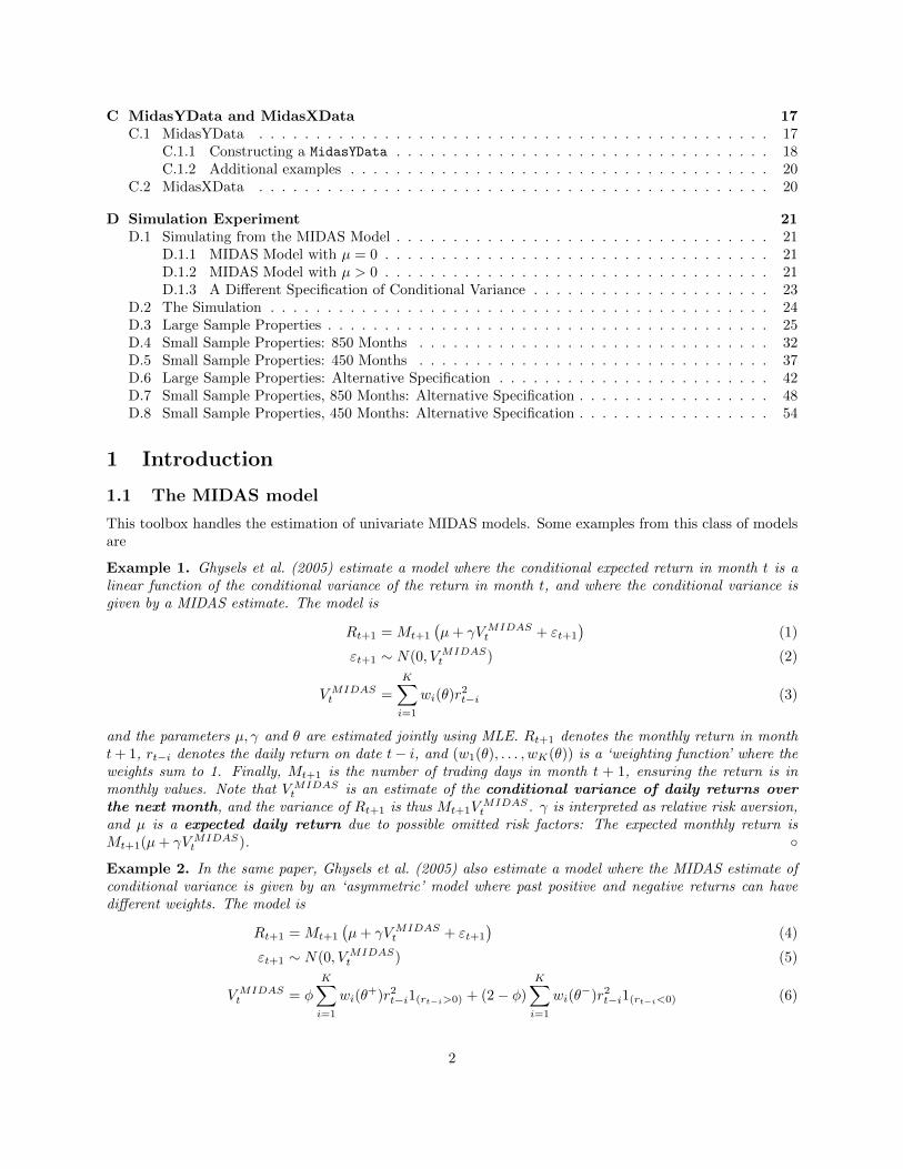
Figure 3 shows the density of r2, r5, r10, r50, and r100 when simulating from the specification (the densities arekernel estimates based on 1,000,000 simulated paths), as well as a typical sample path for rt. The densities forr10 and up are virtually indistinguishable, and the sample path shows clear evidence of volatility clusteringwithout dying out or blowing up.

D.2 The Simulation

I simulate from the model with γ = 0 as I’m primarily interested in the distribution of the parameterestimates under the null of γ = 0. In this case, the volatility of εt is time-varying but the mean of returns isconstant. I choose µ = 0.015 as this keeps the simulated paths roughly stationary (see the above discussion.The time-series is not stationary in theory, but in most samples it behaves as if it were). Simulations wherethe absolute value of a daily return is above 50% are discarded.The weighting scheme used has exponential weights with a 2nd order polynomial, and the simulation exper-iments use use the following parameter values:

µ = 0.015 γ = 0 κ1 = −0.001 κ2 = −0.0001. (82)

24

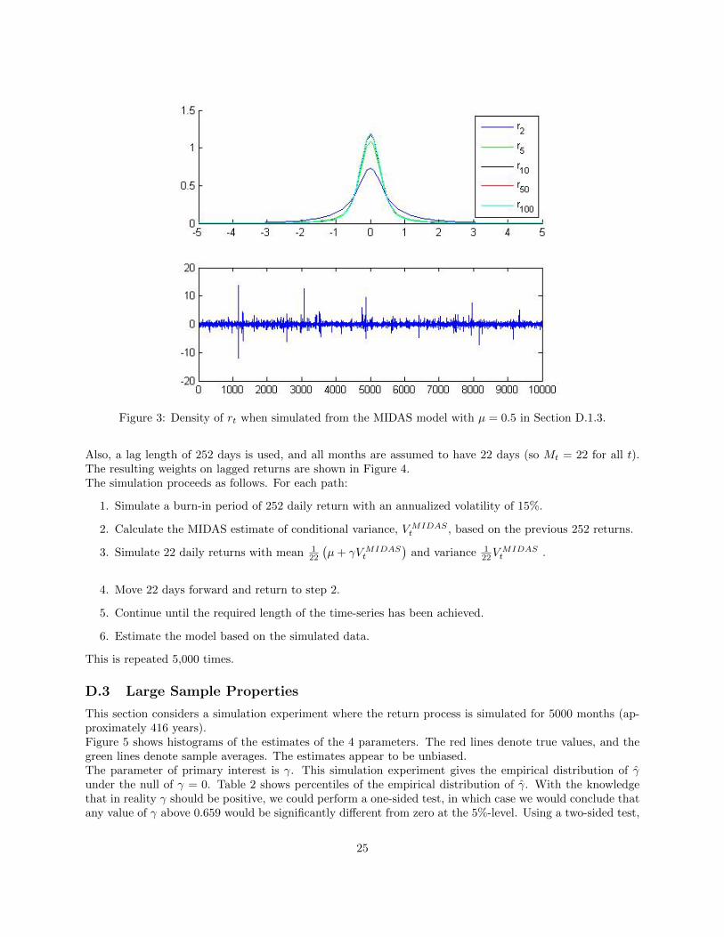
Figure 3: Density of rt when simulated from the MIDAS model with µ = 0.5 in Section D.1.3.

Also, a lag length of 252 days is used, and all months are assumed to have 22 days (so Mt = 22 for all t).The resulting weights on lagged returns are shown in Figure 4.The simulation proceeds as follows. For each path:

1. Simulate a burn-in period of 252 daily return with an annualized volatility of 15%.

2. Calculate the MIDAS estimate of conditional variance, VMIDASt , based on the previous 252 returns.

3. Simulate 22 daily returns with mean 122

(µ+ γVMIDAS

t

)and variance 1

22VMIDASt .

4. Move 22 days forward and return to step 2.

5. Continue until the required length of the time-series has been achieved.

6. Estimate the model based on the simulated data.

This is repeated 5,000 times.

D.3 Large Sample Properties

This section considers a simulation experiment where the return process is simulated for 5000 months (ap-proximately 416 years).Figure 5 shows histograms of the estimates of the 4 parameters. The red lines denote true values, and thegreen lines denote sample averages. The estimates appear to be unbiased.The parameter of primary interest is γ. This simulation experiment gives the empirical distribution of γunder the null of γ = 0. Table 2 shows percentiles of the empirical distribution of γ. With the knowledgethat in reality γ should be positive, we could perform a one-sided test, in which case we would conclude thatany value of γ above 0.659 would be significantly different from zero at the 5%-level. Using a two-sided test,

25

Figure 4: Weights on past returns used in the simulation.

we would conclude that any value of γ above 0.831 would be significantly different from zero (recall that thisis based on 5,000 months of observations).

0.5% 2.5% 5% 10% 90% 95% 97.5% 99.5%γ -1.5271 -1.0031 -0.7845 -0.5692 0.4661 0.6591 0.8309 1.2315

Table 2: Percentiles of the empirical distribution of γ when the model is simulated with γ = 0.

Figure 7 shows histograms of the t-statistics calculated using robust variance estimates for each of the fourparameters. The t-stats using MLE variance estimates based on the Hessian are shown in Figure 8 and 9.Table 3 shows the variance of the estimates from the simulation, which can be viewed as the true variance ofthe estimates. Also, the table shows the mean of the robust variance estimates, the MLE Hessian estimateand the MLE score estimate. For γ the robust variance estimate has the smallest bias.I also calculate the rejection rate for the tests µ = µ0, γ = γ0, κ1 = κ10 and κ2 = κ20, where µ0, γ0, κ10and κ20 denote the true parameters used in the simulation. The test is done as a t-test, and the risks ofincorrectly rejecting these hypothesis, a type 1 error, should be 5%. As shown in Table 4, when using robuststandard error, the numbers are 5.74%, 5.10%, 6.20% and 10.52%. So for µ, γ and κ1 a type 1 error occursin approximately 5% of the simulations, but for κ2 a type 1 error occurs more often. When using MLEstandard errors, the rejection rates are a bit higher and thus farther from 5%.To investigate how the precision of the estimates depends on the volatility of the simulated returns, Figure 10first shows a histogram of the annualized volatility of the simulated return processes (calculated as std(r) ·√

250). Most simulations have an annualized volatility between 10 and 20 percent, but for some simulationsthe volatility is higher.Second, Figure 11 plots the estimate for a given simulation as a function of the annualized volatility forthat simulation. The red lines show the true values of the parameters used in the simulations. Clearly, the

26

Figure 5: Parameter estimates for simulated data, when 5000 months of returns are simulated. The red linesdenote true values, the green lines denote sample averages.

True Robust MLE Hessian MLE Scoreµ 2.34e-007 2.36e-007 2.29e-007 2.23e-007Bias 2.49e-009 -4.76e-009 -1.08e-008γ 1.95e-001 1.90e-001 1.86e-001 1.83e-001Bias -4.19e-003 -8.19e-003 -1.11e-002κ1 3.21e-004 4.81e-004 2.93e-004 2.61e-004Bias 1.60e-004 -2.83e-005 -6.04e-005κ2 2.31e-008 3.96e-008 2.14e-008 1.81e-008Bias 1.65e-008 -1.64e-009 -5.01e-009

Table 3: Empirical variance of the simulated estimates (‘true variance’) and the mean of different varianceestimates. The variance estimates are calculated in three ways: Using White’s method (robust); using MLEstandard errors based on the Hessian; and using MLE standard errors based on the score.

estimate of γ becomes more precise when volatility is high. This is intuitive—if volatility is zero, γ is notidentified. It also looks like the estimates of µ, κ1 and κ2 become more precise when volatility is high.Maybe we should look at the conditional distribution of γ given that the volatility of simulatedreturns is btw. something like 10% and 20%. This would make the empirical distribution lesspeaked, and make any given number less significant.

27

Figure 6: Scatter plot of the estimates of κ1 and κ2, showing that these estimates are strongly negativelycorrelated. The red lines show the true values of κ1 and κ2 used for the simulation.

Figure 7: Histogram of t-stats using Robust variance estimates for simulated data, when 5000 months ofreturns are simulated.

28

Figure 8: Histogram of t-stats using MLE variance estimates based on the Hessian for simulated data, when5000 months of returns are simulated.

Figure 9: Histogram of t-stats using MLE variance estimates based on the score for simulated data, when5000 months of returns are simulated.

29

Hypothesis Robust MLE Hessian MLE Scoreµ = µ0 0.0574 0.0608 0.0646γ = γ0 0.0510 0.0542 0.0572κ1 = κ10 0.0620 0.0706 0.0778κ2 = κ20 0.1052 0.1050 0.1174

Table 4: Frequency of type 1 errors (rejection rate for the hypothesis that each parameter equals its truevalue), when 5000 months of returns are simulated. The standard errors of the estimates are calculated inthree ways: Using White’s method (robust); using MLE standard errors based on the Hessian; and usingMLE standard errors based on the score.

Figure 10: Annualized volatility for each of the 5000 simulations, when 5000 months of returns are simulated.

30

Figure 11: Parameter estimates as a function of the annualized volatility of the simulated return process,when 5000 months of returns are simulated.

31

D.4 Small Sample Properties: 850 Months

This section considers a simulation experiment where the return process is simulated for 850 months (ap-proximately the sample length available from CRSP). The simulation is repeated 5000 times. Figure 12shows histograms of the estimates of the 4 parameters. The red lines denote true values, and the green linesdenote sample averages. As before the estimates of µ and γ appear to be unbiased. However, the estimatesof κ1 and κ2 now have a small bias due to outliers.


Table 5 shows percentiles of the empirical distribution of γ. With the knowledge that in reality γ shouldbe positive, we could perform a one-sided test, in which case we would conclude that any value of γ above2.17 would be significantly different from zero. Using a two-sided test, we would conclude that any valueof γ above 2.80 would be significantly different from zero. Ghysels, Santa-Clara and Valkanov (2005) findγ = 2.606 with a t-stat of 6.7 using data from 1928 to 2000.

0.5% 2.5% 5% 10% 90% 95% 97.5% 99.5%γ -5.6233 -3.7061 -2.8742 -2.0525 1.5130 2.1704 2.8015 4.2306


Figure 14 shows histograms of the t-stats using robust variance estimates for each of the four parameters.Histograms of the t-stats using MLE variance estimates based on the Hessian and score are shown in Figure 15and 16.Table 6 shows the variance of the estimates from the simulation, which can be viewed as the true variance ofthe estimates. Also, the table shows the mean of the robust variance estimates, the MLE Hessian estimateand the MLE score estimate. For γ the robust variance estimate now has the largest bias.

32


Figure 14: Histograms of t-stats using Robust variance estimates for simulated data, when 850 months ofreturns are simulated.

33

True Robust MLE Hessian MLE Scoreµ 3.97e-006 4.01e-006 3.72e-006 3.59e-006Bias 4.09e-008 -2.51e-007 -3.82e-007γ 2.44e+000 2.55e+000 2.45e+000 2.46e+000Bias 1.14e-001 1.67e-002 1.95e-002κ1 2.71e-002 4.74e-002 1.29e-002 9.25e-003Bias 2.04e-002 -1.41e-002 -1.78e-002κ2 1.90e-006 5.42e-006 1.19e-006 8.06e-007Bias 3.52e-006 -7.04e-007 -1.09e-006

Table 6: Empirical variance of the simulated estimates (‘true variance’) and the mean of different varianceestimates, when simulating 850 months of returns. The variance estimates are calculated in three ways:Using White’s method (robust); using MLE standard errors based on the Hessian; and using MLE standarderrors based on the score.

I also calculate the rejection rate for the tests µ = µ0, γ = γ0, κ1 = κ10 and κ2 = κ20, where µ0, γ0, κ10and κ20 denote the true parameters used in the simulation. The test is done as a t-test, and the risks ofincorrectly rejecting these hypothesis, a type 1 error, should be 5%. As shown in Table 7 the numbers are5.32%, 4.84%, 7.34% and 11.54% using robust standard errors. So, as with 5000 months of simulated return,for µ, γ and κ1 a type 1 error occurs in approximately 5% of the simulations, but for κ2 a type 1 error occursmore often. The robust standard errors no longer perform the best across all parameters.To investigate how the precision of the estimates depends on the volatility of the simulated returns, Figure 17first shows the annualized volatility of the simulated return processes (calculated as std(r) ·

√250). Most

simulations have an annualized volatility between 10 and 20 percent, but for some simulations the volatilityis higher.Second, Figure 18 plots the estimate for a given simulation as a function of the annualized volatility for

Figure 15: Histograms of t-stats using MLE variance estimates based on the Hessian for simulated data,when 850 months of returns are simulated.

34

Figure 16: Histograms of t-stats using MLE variance estimates based on the score for simulated data, when850 months of returns are simulated.



that simulation. The red lines show the true values of the parameters used in the simulations. Clearly, theestimate of γ becomes more precise when volatility is high. It also looks like the estimates of µ, κ1 and κ2become more precise when volatility is high. Maybe we should look at the conditional distributionof γ given that the volatility of simulated returns is btw. something like 10% and 20%.

35



36

D.5 Small Sample Properties: 450 Months

Finally, this section considers a simulation experiment where the return process is simulated for 450 months(approximately half of the period available from CRSP). Figure 19 shows histograms of the estimates of the4 parameters. The red lines denote true values, and the green lines denote sample averages. As before theestimates of µ and γ appear to be unbiased. However, the estimates of κ1 and κ2 now have a some bias dueto outliers.


Table 8 shows percentiles of the empirical distribution of γ. With the knowledge that in reality γ shouldbe positive, we could perform a one-sided test, in which case we would conclude that any value of γ above3.42 would be significantly different from zero. Using a two-sided test, we would conclude that any valueof γ above 4.56 would be significantly different from zero. Ghysels, Santa-Clara and Valkanov (2005) findγ = 1.547 with a t-stat of 3.38 using data from 1928 to 1963, and γ = 3.748 with a t-stat of 8.61 using datafrom 1964 to 2000.

0.5% 2.5% 5% 10% 90% 95% 97.5% 99.5%γ -8.2602 -5.8820 -4.6321 -3.3683 2.4321 3.4188 4.5578 6.7694


Figure ?? shows histograms of the t-stats using robust variance estimates for each of the four parameters.The t-stats using MLE variance estimates based on the Hessian and score are shown in Figure ?? and ??.Table 9 shows the variance of the estimates from the simulation, which can be viewed as the true variance ofthe estimates. Also, the table shows the mean of the robust variance estimates, the MLE Hessian estimateand the MLE score estimate. As with 850 months of observations, the robust variance estimate has the

37


Figure 21: Histograms of t-stats using robust variance estimates for simulated data, when 450 months ofreturns are simulated.

38


largest bias for γ.I also calculate the rejection rate for the tests µ = µ0, γ = γ0, κ1 = κ10 and κ2 = κ20, where µ0, γ0, κ10and κ20 denote the true parameters used in the simulation. The test is done as a t-test, and the risks of


39

True Robust MLE Hessian MLE Scoreµ 1.38e-005 1.38e-005 1.21e-005 1.15e-005Bias -7.48e-008 -1.78e-006 -2.30e-006γ 6.09e+000 6.44e+000 5.92e+000 5.98e+000Bias 3.55e-001 -1.63e-001 -1.09e-001κ1 3.75e-001 7.46e-001 1.82e-001 1.38e-001Bias 3.71e-001 -1.93e-001 -2.37e-001κ2 1.93e-005 2.83e-005 1.01e-005 7.82e-006Bias 8.95e-006 -9.23e-006 -1.15e-005


incorrectly rejecting these hypothesis, a type 1 error, should be 5%. As shown in Table 10 the numbers are5.16%, 5.52%, 9.40% and 12.58% using robust standard errors. As before, for µ and γ a type 1 error occursin approximately 5% of the simulations, but for both κ1 and κ2 a type 1 error occurs more often.



To investigate how the precision of the estimates depends on the volatility of the simulated returns, Figure 24first shows the annualized volatility of the simulated return processes (calculated as std(r) ·

√250). Most

simulations have an annualized volatility between 10 and 20 percent, but for some simulations the volatilityis higher, sometimes as high as 80% annualized.Second, Figure 25 plots the estimate for a given simulation as a function of the annualized volatility forthat simulation. The red lines show the true values of the parameters used in the simulations. Clearly, theestimate of γ becomes more precise when volatility is high, and this is now also clearly the case for theestimates of κ1 and κ2. Maybe we should look at the conditional distribution of γ given that thevolatility of simulated returns is btw. something like 10% and 20%.

40



41

D.6 Large Sample Properties: Alternative Specification

I now consider the alternative specification of variance, in which

VMIDASt = ω + δ

K∑t=0

wi(θ)r2t−i. (83)

The unconditional variance is given by ω/(1−δ). Hence, I simulate the model by specifying the unconditionalvolatility to be 15% annualized and let the variance be given by

VMIDASt = V ar(r)(1− δ) + δ

K∑t=0

wi(θ)r2t−i. (84)

Next, I also estimate the model using this specification, which only requires estimating δ and not ω (this issometimes known as ‘volatility targeting’ and is also common when estimating GARCH models).Because δ is required to be in (0, 1) to ensure a positive variance, I use the transformation δ = exp(φ)/(1 +exp(φ) where φ ∈ (−∞,∞). For the simulations I choose φ = 1 which corresponds to δ = 0.7311.When simulating using this specification, the return process no longer blows up or dies out. Hence, I nowtake µ = 0, but keep the other parameters as before. Thus,

µ = 0.0 γ = 0.0 κ1 = −0.001 κ2 = −0.0001 φ = 1 (85)

This section considers a simulation experiment where the return process is simulated for 5000 months (ap-proximately 416 years).Figure 26 shows histograms of the estimates of the 4 parameters. The red lines denote true values, and thegreen lines denote sample averages. The figure now includes a histogram of the estimates of φ. All estimatesappear to be unbiased.The parameter of primary interest is γ. This simulation experiment gives the empirical distribution of γunder the null of γ = 0. Table 11 shows percentiles of the empirical distribution of γ. With the knowledgethat in reality γ should be positive, we could perform a one-sided test, in which case we would concludethat any value of γ above 1.15 would be significantly different from zero at the 5%-level. Using a two-sidedtest, we would conclude that any value of γ above 1.38 would be significantly different from zero (recall thatthis is based on 5,000 months of observations). Note that the distribution of γ found for this specificationof the MIDAS model is much wider than before. Think about why: is it because volatility is loweron average, or is it because vol of vol is different?

0.5% 2.5% 5% 10% 90% 95% 97.5% 99.5%γ -1.9553 -1.4784 -1.2061 -0.9278 0.9046 1.1532 1.3804 1.7734


Figure 27 shows histograms of the t-stats using robust variance estimates for each of the four parameters,and the t-stats using MLE variance estimates based on the Hessian and score are shown in Figure 28 and29.Table 12 shows the variance of the estimates from the simulation, which can be viewed as the true varianceof the estimates. Also, the table shows the mean of the robust variance estimates, the MLE Hessian estimateand the MLE score estimate. The size of the bias is an order of magnitude smaller than the mean.I also calculate the rejection rate for the tests µ = µ0, γ = γ0, κ2 = κ20 and φ = φ0, where µ0, γ0, κ20, and φ0denote the true parameters used in the simulation. The test is done as a t-test, and the risks of incorrectlyrejecting these hypothesis, a type 1 error, should be 5%. As shown in Table 13, when using robust standarderror, the numbers are 4.86%, 4.78%, 4.76%, 6.88% and 3.66%.Figure 30 shows the annualized volatility of the simulated return processes (calculated as std(r) ·

√250).

With this specification of the conditional variance, the simulated variance is always close to the target of15%.

42

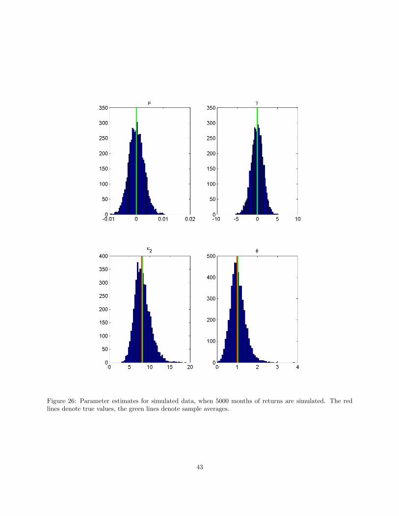
Figure 26: Parameter estimates for simulated data, when 5000 months of returns are simulated. The redlines denote true values, the green lines denote sample averages.

43


True Robust MLE Hessian MLE Scoreµ 7.88e-006 7.96e-006 7.82e-006 7.84e-006Bias 8.57e-008 -5.28e-008 -3.13e-008γ 2.14e+000 2.17e+000 2.13e+000 2.14e+000Bias 2.62e-002 -1.14e-002 -5.24e-003κ2 3.82e+000 4.40e+000 3.87e+000 3.75e+000Bias 5.79e-001 5.35e-002 -7.11e-002φ 1.38e-001 1.43e-001 1.39e-001 1.38e-001Bias 4.59e-003 4.80e-004 7.04e-005

Table 12: Empirical variance of the simulated estimates (‘true variance’) and the mean of different varianceestimates. The variance estimates are calculated in three ways: Using White’s method (robust); using MLEstandard errors based on the Hessian; and using MLE standard errors based on the score.

44


Hypothesis Robust MLE Hessian MLE Scoreµ = µ0 0.0478 0.0488 0.0482γ = γ0 0.0476 0.0486 0.0480κ2 = κ20 0.0688 0.0652 0.0696φ = φ0 0.0366 0.0382 0.0392


45


46


47

D.7 Small Sample Properties, 850 Months: Alternative Specification

This section considers a simulation experiment where the return process is simulated for 850 months (approx-imately the sample length available from CRSP). The simulation is repeated 5000 times. Figure 31 showshistograms of the estimates of the 5 parameters as well as the annualized volatility of the simulated returns.The red lines denote true values, and the green lines denote sample averages. As before the estimates of µand γ appear to be unbiased. Because of the transformation φ = exp(φ)/(1 + exp(φ)), the estimate of φ nowhas a cluster between 10 and 15, which corresponds to φ ≈ 1. This is, the optimizer would really like to driveφ above 1, but because of the restriction 0 < φ < 1 the estimates instead cluster around 1, corresponding tolarge values of φ between 10 and 15.Table 14 shows percentiles of the empirical distribution of γ, which is now much wider than before. With theknowledge that in reality γ should be positive, we could perform a one-sided test, in which case we wouldconclude that any value of γ above 6.59 would be significantly different from zero. Using a two-sided test,we would conclude that any value of γ above 7.95 would be significantly different from zero.

0.5% 2.5% 5% 10% 90% 95% 97.5% 99.5%γ -12.8724 -8.5316 -6.5524 -4.9517 4.9736 6.5850 7.9501 12.1776


Figure 32 shows histograms of the t-stats using robust variance estimates for each of the four parameters,and the t-stats using MLE variance estimates based on the Hessian and score are shown in Figure 33 and34.Table 15 shows the variance of the estimates from the simulation, which can be viewed as the true varianceof the estimates. Also, the table shows the mean of the robust variance estimates, the MLE Hessian estimateand the MLE score estimate. For µ and γ the bias of the variance estimates is an order of magnitude smallerthan the variance itself. However, for κ2 and φ the bias in the variance is significant.

True Robust MLE Hessian MLE Scoreµ 6.46e-005 8.92e-005 6.79e-005 6.32e-005Bias 2.46e-005 3.29e-006 -1.40e-006γ 1.76e+001 2.38e+001 1.83e+001 1.72e+001Bias 6.24e+000 7.23e-001 -4.54e-001κ2 9.81e+001 1.62e+002 7.69e+001 8.73e+001Bias 6.42e+001 -2.12e+001 -1.08e+001φ 6.53e+000 4.74e+001 5.52e+003 6.22e+008Bias 4.08e+001 5.51e+003 6.22e+008


I also calculate the rejection rate for the tests µ = µ0, γ = γ0, κ2 = κ20, and φ = φ0 where µ0, γ0, κ10,and φ0 denote the true parameters used in the simulation. The test is done as a t-test, and the risks ofincorrectly rejecting these hypothesis, a type 1 error, should be 5%. As shown in Table 16 the numbers are3.24%, 3.02%, 15.14% and 7.44% using robust standard errors. So, as with 5000 months of simulated return,for µ, γ and κ1 a type 1 error occurs in approximately 5% of the simulations, but for κ2 a type 1 error occursmore often.Figure 35 shows the annualized volatility of the simulated return processes (calculated as std(r) ·

√250).

48


49




50


51


52


53

D.8 Small Sample Properties, 450 Months: Alternative Specification

Finally, this section considers a simulation experiment where the return process is simulated for 450 months(approximately half of the period available from CRSP). Figure 36 shows histograms of the estimates of the4 parameters. The red lines denote true values, and the green lines denote sample averages. As before theestimates of µ and γ appear to be unbiased. However, the estimates of κ2 now have a some bias due tooutliers, and the estimate of φ is heavily biased due to the clustering of estimates around 10-15 (correspondingto δ ≈ 1). For both µ, γ and κ2 we also see some clustering of estimates close to the boundaries I’ve imposedwhen doing the optimization.


54

Table 17 shows percentiles of the empirical distribution of γ, which is now very wide. With the knowledgethat in reality γ should be positive, we could perform a one-sided test, in which case we would concludethat any value of γ above 9.85 would be significantly different from zero. Using a two-sided test, we wouldconclude that any value of γ above 13.13 would be significantly different from zero.

0.5% 2.5% 5% 10% 90% 95% 97.5% 99.5%γ -48.8653 -14.8473 -10.8029 -7.4182 7.3999 9.8503 13.1344 32.7321


Figure 37 shows histograms of the t-stats using robust variance estimates for each of the four parameters,and the t-stats using MLE variance estimates based on the Hessian and score are shown in Figure 38 and39.Table 18 shows the variance of the estimates from the simulation, which can be viewed as the true varianceof the estimates. Also, the table shows the mean of the robust variance estimates, the MLE Hessian estimateand the MLE score estimate. There is now a heavy bias in all variance estimates due to outliers!

True Robust MLE Hessian MLE Scoreµ 2.37e-004 8.99e-002 -2.70e-001 4.43e+005Bias 8.96e-002 -2.71e-001 4.43e+005γ 6.47e+001 2.45e+004 -7.79e+004 1.17e+011Bias 2.45e+004 -7.80e+004 1.17e+011κ2 4.21e+002 5.29e+003 -3.63e+006 1.63e+013Bias 4.87e+003 -3.63e+006 1.63e+013φ 1.63e+001 1.31e+002 2.40e+004 3.58e+010Bias 1.14e+002 2.40e+004 3.58e+010


I also calculate the rejection rate for the tests µ = µ0, γ = γ0, κ2 = κ20, and φ = φ0, where µ0, γ0, κ20,and φ0 denote the true parameters used in the simulation. The test is done as a t-test, and the risks ofincorrectly rejecting these hypothesis, a type 1 error, should be 5%. As shown in Table 19 the numbersare 2.54%, 2.44%, 18.70% and 13.78% using robust standard errors. For µ and γ a type 1 error occurs inapproximately 2.5% the simulations—half of the target frequency, but for κ2 a type 1 error occurs moreoften, and for φ it depends on the variance estimate used.



Figure 40 shows the annualized volatility of the simulated return processes (calculated as std(r) ·√

250).

55


References

Ghysels, E., P. Santa-Clarab, and R. Valkanov (2005). There is a risk-return trade-off after all. Journal ofFinancial Economics 76, 509–548.

56


57


58


59

Documents

MIDAS MatLab Toolbox - NYU Stern School of Businesspages.stern.nyu.edu/~ehedegaa/PDFs/MidasManual.pdf · MIDAS MatLab Toolbox Esben Hedegaardy August 29, 2011 ... following code (it’s