HAL Id: hal-00705536https://hal.archives-ouvertes.fr/hal-00705536

Submitted on 18 Dec 2015

HAL is a multi-disciplinary open accessarchive for the deposit and dissemination of sci-entific research documents, whether they are pub-lished or not. The documents may come fromteaching and research institutions in France orabroad, or from public or private research centers.

L’archive ouverte pluridisciplinaire HAL, estdestinée au dépôt et à la diffusion de documentsscientifiques de niveau recherche, publiés ou non,émanant des établissements d’enseignement et derecherche français ou étrangers, des laboratoirespublics ou privés.

Mid-tropospheric δD observations from IASI/MetOp athigh spatial and temporal resolution

Jean-Lionel Lacour, Camille Risi, Lieven Clarisse, Sandrine Bony, DanielHurtmans, Cathy Clerbaux, Pierre-François Coheur

To cite this version:Jean-Lionel Lacour, Camille Risi, Lieven Clarisse, Sandrine Bony, Daniel Hurtmans, et al.. Mid-tropospheric δD observations from IASI/MetOp at high spatial and temporal resolution. AtmosphericChemistry and Physics, European Geosciences Union, 2012, 12 (22), pp.10817-10832. �10.5194/acp-12-10817-2012�. �hal-00705536�

Atmos. Chem. Phys., 12, 10817–10832, 2012www.atmos-chem-phys.net/12/10817/2012/doi:10.5194/acp-12-10817-2012© Author(s) 2012. CC Attribution 3.0 License.

AtmosphericChemistry

and Physics

Mid-tropospheric δD observations from IASI/MetOpat high spatial and temporal resolution

J.-L. Lacour1, C. Risi2, L. Clarisse1, S. Bony2, D. Hurtmans1, C. Clerbaux3,1, and P.-F. Coheur1

1Spectroscopie de l’Atmosphere, Service de Chimie Quantique et Photophysique,Universite Libre de Bruxelles, Belgium2LMD/IPSL, CNRS, Paris, France3UPMC Univ. Paris 06, Universite Versailles St.-Quentin, CNRS/INSU, LATMOS-IPSL, Paris, France

Correspondence to:J.-L. Lacour (jlacour@ulb.ac.be)

Received: 18 April 2012 – Published in Atmos. Chem. Phys. Discuss.: 25 May 2012Revised: 12 October 2012 – Accepted: 23 October 2012 – Published: 16 November 2012

Abstract. In this paper we retrieve atmospheric HDO, H2Oconcentrations and their ratioδD from IASI radiances spec-tra. Our method relies on an existing radiative transfer model(Atmosphit) and an optimal estimation inversion scheme, butgoes further than our previous work by explicitly consider-ing correlations between the two species. A global HDO andH2O a priori profile together with a covariance matrix werebuilt from daily LMDz-iso model simulations of HDO andH2O profiles over the whole globe and a whole year. The re-trieval parameters are described and characterized in termsof errors. We show that IASI is mostly sensitive toδD inthe middle troposphere and allows retrievingδD for an inte-grated 3–6 km column with an error of 38 ‰ on an individ-ual measurement basis. We examine the performance of theretrieval to capture the temporal (seasonal and short-term)and spatial variations ofδD for one year of measurement attwo dedicated sites (Darwin and Izana) and a latitudinal bandfrom −60◦ to 60◦ for a 15 day period in January. We reporta generally good agreement between IASI and the model andindicate the capabilities of IASI to reproduce the large scalevariations ofδD (seasonal cycle and latitudinal gradient) withgood accuracy. In particular, we show that there is no system-atic significant bias in the retrievedδD values in comparisonwith the model, and that the retrieved variability is similar tothe one in the model even though there are certain local dif-ferences. Moreover, the noticeable differences between IASIand the model are briefly examined and suggest modeling is-sues instead of retrieval effects. Finally, the results further re-veal the unprecedented capabilities of IASI to capture short-term variations inδD, highlighting the added value of thesounder for monitoring hydrological processes.

1 Introduction

Water vapor is a key gas for the climate system. It is thestrongest absorber of infrared radiation in our atmosphere,contributing to approximately 50 % of the total greenhouseeffect (Schmidt et al., 2010; Kiehl and Trenberth, 1997).Moist processes also play a key role in controlling the large-scale atmospheric circulation (Randall et al., 1989; Frierson,2007) and its sensitivity to climate forcing (Kang et al., 2008;Zhang et al., 2010). Even though hydrological processes havebeen studied abundantly, there is still an insufficient under-standing of the factors controlling water amount (Sherwoodet al., 2010; Schneider et al., 2010b). As major climate feed-backs (cloud and water vapor feedbacks) are associated withtropospheric water vapor (Soden and Held, 2006; Bony et al.,2006), there is a need to better assess the mechanisms thatcontrol the humidity distribution in the troposphere.

Because vapor pressure depends on the mass of the watermolecules, there is a fractionation of the different isotopo-logues during evaporation and condensation processes: heav-ier isotopologues (H218O, H2

17O and HDO) have a lowervapor pressure and will preferentially condensate, leadingto a depletion of the heavier isotopologues in an airmassthat experiences condensation. The isotopic composition ofan air parcel therefore gives a fingerprint of the history ofthe phase changes. Because the factors that control the wa-ter vapor amount also control the isotopic fractionation ofthe air parcel, an accurate measurement of isotopologues ra-tio is invaluable for the study of humidity processes. Mea-surements from various instruments (cavity ring down spec-trometers, ground-based FTIR, atmospheric sounders) have

Published by Copernicus Publications on behalf of the European Geosciences Union.

10818 J.-L. Lacour et al.: Mid-tropospheric δD observations from IASI/MetOp

demonstrated this and have been used to examine, for in-stance, air mass mixing (Noone et al., 2011), transport pro-cesses (Strong et al., 2007), evaporation of hydro-meteors(Worden et al., 2007), cloud processes (Lee et al., 2011) andintra-seasonal climate variability in the tropics (Kurita et al.,2011; Berkelhammer et al., 2012). Isotopic concentrationsare commonly expressed asδ values that define the relativedeviation of the ratio with respect to a standard ratio. Forexample, the concentration in HDO with respect to H2O isexpressed as

δD = 1000

( HDOH2O

VSMOW− 1

), (1)

where VSMOW (Vienna Standard Mean Ocean Water) is thereference standard for water isotope ratios (Craig, 1961).

Today, several space-borne instruments can capture iso-topic variations. The Tropospheric Emission Spectrometer(TES) and the SCanning Imaging Absorption spectroMe-ter for Atmospheric CartograpHY (SCIAMACHY) instru-ments have been the first to provide global distributions ofδD representative of the mid-troposphere (Worden et al.,2006, 2007) and the boundary layer (Frankenberg et al.,2009), respectively. The inter comparisons of observationswith isotopologues-enabled atmospheric general circulationmodels have demonstrated the added value of such measure-ments to identify biases in the modeling of the isotopic frac-tionation and thus to better characterize hydrological pro-cesses (Risi et al., 2010a, 2012a,b; Yoshimura et al., 2011).

Two other space-based remote sensing instruments canmeasure the isotopic composition in the troposphere: theInfrared Atmospheric Sounding Interferometer on boardMetOp (Clerbaux et al., 2009) and the Thermal And Nearinfrared Sensor for carbon Observation (TANSO) on boardGOSAT (C. Frankenberg, personal communication, 2012).IASI is especially attractive for this purpose, considering itsunprecedented spatial coverage and temporal sampling (seebelow), and the long-term character of the mission with 15 yrof planned continuous data. The potential of IASI to measureδD was first investigated byHerbin et al.(2009) who car-ried out a sensitivity study. More recently retrievals ofδDapplying IASI spectra have been presented and comparedto ground-based FTIR measurements (Schneider and Hase,2011).

This paper focuses on the retrieval ofδD from IASIspectral radiances and their evaluation. Tropospheric watervapour concentrations are very variable, while the HDO/H2Oratio is rather stable in comparison. For measuring watervapour isotopologues ratios, we thus need a technique that issensitive over a large dynamic range, and at the same timeprecise enough to capture small isotopic variations. Sinceit is difficult for any measurement technique to optimallymeet both requirements; tropospheric water vapor isotopo-logues ratio measurements are very difficult. We use a ra-diative transfer model that is similar to the one used in the

Herbin et al.(2009) study. Their retrieval was based on a si-multaneous but independent retrieval of H2

16O and HDO.Here we constrain the retrieval with a full covariance matrixthat takes into account the correlations between H2

16O andHDO. This new retrieval methodology named the HDO/H2Ocorrelated approach is described in Sect. 3. In that section wealso extensively characterize the retrievals in terms of verticalsensitivity and errors. In Sect. 2 we first briefly recall someof the main IASI characteristics. In Sect. 4 we describe thefirst retrieval results, focusing on the ability of IASI to cap-ture theδD seasonal cycle but also rapid temporal variationsat two sites (Izana 28◦18′ N 16◦29′ W, and Darwin 12◦27′ S130◦50′ E), as well as latitudinal variations over the globe.The retrievals are evaluated by comparing the retrieved val-ues to those modeled by the LMDz-iso General CirculationModel (GCM) (Risi et al., 2010b).

2 IASI observations

IASI is a Fourier transform spectrometer on board theMETOP series of European meteorological polar-orbit satel-lites. The first model, designed to provide 5 yr of global-scaleobservations, was launched in October 2006. A second anda third instrument will be launched in 2012 and 2016, re-spectively. IASI measures a large part of the thermal infraredspectral region (645–2760 cm−1) continuously at a mediumspectral resolution (0.5 cm−1 apodized). It has a low noise of0.1–0.2 K for a reference blackbody at 280 K, with the lowernoise values in the useful range forδD retrievals (Hiltonet al., 2012). Primarily designed for operational meteoro-logical soundings with a high level of accuracy, the instru-ment achieves a global coverage twice a day (orbits crossingthe Equator at 09:30 and 21:30 LT) with a relatively smallpixel size of 12 km diameter at nadir, larger at off nadir view-ing angles. IASI makes about 1.3 million measurements perday and coping with this volume of data is very challeng-ing, requiring important computing resources coupled witha fast radiative transfer model (e.g.,Hurtmans et al., 2012).In this study we primarily aim at characterizing the newδDretrievals and therefore we have analyzed observations overselected regions.

The main isotopologues of water (H216O, H2

18O andHDO) have large absorption bands in the thermal infraredregion (Rothman et al., 2003; Toth, 1999). Spectral signa-tures of these species are well detected by IASI (Herbinet al., 2009) despite the instrument’s medium spectral res-olution. δ18O retrievals remain challenging as its small vari-ations in the atmosphere require very high accuracy.δD vari-ations are larger by one order of magnitude and are there-fore targeted here. Figure1 shows part of an IASI spec-trum with the spectral windows used in the retrieval (redcurve). These have been chosen to avoid major interferencesof CH4 and N2O in this range. Note that these two smallspectral ranges differ from the large spectral range approach

Atmos. Chem. Phys., 12, 10817–10832, 2012 www.atmos-chem-phys.net/12/10817/2012/

J.-L. Lacour et al.: Mid-tropospheric δD observations from IASI/MetOp 10819

1195 1200 1205 1210 1215 1220 1225 1230 1235 1240 1245 1250

-4.0x10-6-2.0x10-6

0.02.0x10-64.0x10-63.0x10-4

4.0x10-4

5.0x10-4

6.0x10-4

Wavenumbers [cm-1]

R

adia

nce

W c

m-1

sr-1 /

cm-1

Observed spectrum Calculated spectrum Residual

1160 1180 1200 1220 1240 1260 1280 130020

40

60

80

100

N2O simulated transmittance

CH4 simulated transmittance

Tran

smitt

ance

260

280

300

observed spectrum

Brig

htne

ss T

[K]

Fig. 1. Spectral window used in the retrieval. Top panel: IASI spectra (black curve) in brigthness temperature with the spectral signature ofCH4 and N2O. Bottom panel: example of an IASI observed spectra (blue curve), the calculated spectrum (red curve) and the residual (greencurve). The gap between 1223 and 1251 cm−1 avoids major CH4 and N2O interferences.

of Schneider and Hase(2011), which was selected to maxi-mize the level of information. The chosen channels include asufficient number of baseline channels needed to fit the watercontinuum, but at the same time optimize the computationaltime.

3 Retrieval methodology

To retrieveδD from IASI spectral radiances we used the opti-mal estimation method, mainly following the approach pro-posed byWorden et al.(2006) andSchneider et al.(2006).It involves retrieving HDO and H2O with an a priori covari-ance matrix that represents the variability of the two speciesbut also contains information on the correlations betweenthem. The retrieval performed on a log scale allows bet-ter constraint of the solution and minimization of error onthe δD profile (Worden et al., 2006; Schneider et al., 2006;Schneider and Hase, 2011). The line-by-line radiative trans-fer model software Atmosphit developed at the UniversiteLibre de Bruxelles and used in our first attempt to retrieveδD from IASI (Herbin et al., 2009) has been adapted to al-low this HDO/H2O correlated approach.

Using correlations between log(HDO) and log(H2O) helpsto constrain the joint HDO/H2O retrieval to a physicallymeaningful solution, as demonstrated on TES measurements(Worden et al., 2006, 2007, 2012), ground based measure-ments (Schneider et al., 2010a, 2006), and a limited number

of IASI measurements (Schneider and Hase, 2011). How-ever, it is anticipated that the retrieval will greatly dependon the choices of the retrieval setup. We discuss our choiceof a priori constraint specifically in Sect. 3.3. The choice ofretrieval parameters also affects the vertical resolution andthe error budget associated to the retrieval; this is discussedin Sect. 3.2.

3.1 General description

An atmospheric state vector can be related analytically toa corresponding measurement vector using a forward func-tion describing the physics of the measurement. This rela-tionship can be written as

y = F(x,b) + ε, (2)

wherey is the measurement vector (in our case, the IASI ra-diances),ε the instrumental noise,x the state vector that con-tains the parameters to be retrieved, andb the vector contain-ing all other model parameters impacting the measurement(for instance, interfering species, pressure and temperatureprofiles).F is the forward function.

In the case of a linear problem, the maximum a posteriorisolution can be written perRodgers(2000) as

x = xa+ (KT S−1ε K + S−1

a )−1KT S−1ε (y − Kxa), (3)

wherexa is the a priori state vector andK is the Jacobian con-taining the partial derivatives of the forward model elements

www.atmos-chem-phys.net/12/10817/2012/ Atmos. Chem. Phys., 12, 10817–10832, 2012

10820 J.-L. Lacour et al.: Mid-tropospheric δD observations from IASI/MetOp

with respect to the state vector element

K ij =∂Fi(x)

∂xj

. (4)

Sε is the measurement error covariance, andSa is the a prioricovariance matrix. The retrieved state is therefore a combi-nation of the measurement and the a priori state inverselyweighted by their respective covariance matrices.

Retrieving atmospheric quantities from space measure-ments is often a non-linear problem that requires numeri-cal methods to solve. For a moderately non-linear problem,which is the case here, the best estimate of the state vectorcan be found by iteration of

xi+1 = xi + (S−1a + KT

i S−1ε K i)

−1KTi S−1

ε

[y − F(xi) + K i(xi − xa)]. (5)

3.2 Retrieval parameters

We retrieve profiles of HDO and H216O of the 10 first kilo-meters of the atmosphere in 10 discretized layers of 1 kmthickness. The corresponding a priori profile is kept fixed intime and in space. The atmosphere from 10 to 24 km is de-fined and varies according to the EUMETSAT L2 water va-por profiles. We do not retrieve HDO and H2

16O in this upperrange of the atmosphere because in the spectral range used(from 1193 to 1223 cm−1 and from 1251 to 1253 cm−1);variations of the water concentrations fixed from the EU-METSAT L2 water product do not significantly affect themeasurement. We note that our vertical grid is coarser thanthat used in previous studies (Schneider and Hase, 2011;Worden et al., 2012) so that some small improvements maybe provided by using a finer griding; this at the cost of alonger calculation time. Methane (retrieved as a column) aswell as surface temperature are also part of the state vector.We do not retrieve the temperature profiles as inSchneiderand Hase(2011) and we instead use EUMETSAT L2 pro-cessor temperature profiles retrieved for each IASI field ofview (Schlussel et al., 2005), estimated with an error of 1.5 Kat the surface, 0.6 K between 800 and 300 mb and 1.5 K inthe tropopause (Pougatchev et al., 2009). Spectrally resolvedsurface emissivities (on IASI sampling) are explicitly con-sidered above land surfaces, using the monthly climatologyof Zhou et al.(2011). We approximated the measurementnoise covariance matrix as a diagonal matrix with an error1σ of 8× 10−9W/(cm2cm−1sr). Only spectra with an EU-METSAT’s level 2 cloud fraction below 10 % have been con-sidered in this study.

3.3 The a priori information

Retrieving the state vectorx from Eq. (3) is in general an ill-posed problem and to obtain a physical meaningful solutionwe need to constrain the retrieval with a prior information. Inthe optimal estimation framework, the a priori information is

a measure of the knowledge of the state vector prior to themeasurement. The usual approach is to assume a Gaussiandistribution of the state vector, which can then be character-ized by a mean and covariance matrix. The covariance matrixdescribes to which extent parameters co-vary, for an ensem-ble ofn vectors{yi}. It is given by

Si,j =

∑i,j

{(yi − y)(yj − y)}/n2. (6)

Its diagonal elements are the variances of the individual pa-rameters.

Here, our state vector contains log(H2O) and log(HDO)

profiles. Within one profile, different altitude levels are cor-related. However, there are also strong correlations betweenlog(H2O) and log(HDO). These correlations can be cap-tured in a total covariance matrixSa, which can naturally begrouped into four sub-blocks as

Sa =

(SH2OL

)1

(S(H2OL ,HDOL)

)3(

S(HDOL ,H2OL)

)4

(SHDOL

)2

, (7)

where the two blocksSH2OL andSHDOL are the covariancematrices of the log(H2O) and log(HDO), respectively. ThematricesS(H2OL ,HDOL) = ST

(HDOL ,H2OL) contain the correla-tions between log(H2O) and log(HDO).

The choice of the a priori information is critical in theregularization of an ill-posed problem (Rodgers, 2000). Thebest way to get adequate prior information is to derive themean and covariance from independent measurements dataat high spatial resolution. Only few measurements ofδD ver-tical profiles (Ehhalt, 1974; Strong et al., 2007) as surfacemeasurements (Galewsky et al., 2007, 2011; Johnson et al.,2011) are available. They are not representative for our pur-pose, which is to retrieveδD profiles over extended areas,covering polar to tropical latitudes. Therefore, to constructa priori information we used outputs from the isotopologues-enabled general circulation model LMDz (Risi et al., 2010b),which has demonstrated reasonably well its capabilities tocapture water vapor and isotopic distributions at seasonal andintra-seasonal time scales (Risi et al., 2010a, 2012b). Thesesimulations were nudged by ECMWF reanalyzed winds tosimulate a day-to-day variability of weather regimes con-sistent with observations. To avoid spatial dependency ofthe results on the a priori profile, a single a priori statevector has been calculated as the mean of an ensembleof HDO and H2O simulated profiles representative of thewhole globe and the whole year. The associated covariances(SHDOL ,SH2OL ,S(H2OL ,HDOL) defined by Eq.7) have beencomputed to build the a priori covariance matrix. The H2O,andδD a priori profiles are plotted in Fig.2.

With the covariance matrix constructed in this way, a sig-nificant number of retrievals failed to converge to a solution.A possible reason for this could lie in the specifics of thecalculation of the numerical derivatives. We found that this

Atmos. Chem. Phys., 12, 10817–10832, 2012 www.atmos-chem-phys.net/12/10817/2012/

J.-L. Lacour et al.: Mid-tropospheric δD observations from IASI/MetOp 10821

0.0 0.1 0.2 0.3 0.40

1

2

3

4

5

6

7

8

9

10

50 100 150 200 250 300 0.01 0.1 1 100

1

2

3

4

5

6

7

8

9

10

-500 -400 -300 -200 -100 00

1

2

3

4

5

6

7

8

9

10

original LMDz 1 modified 1

c)A priori D [per mil]

A priori H2O variability 1 [%]

Approximated a priori variability in per mil

A priori H2O [g/kg]

SR

1/2

original LMDz 1 approximated original LMDz 1 approximated modified 1

d)

b)

80 100 120 140 160

apriori D profile

a)

Fig. 2.Description of a priori information.(a) A priori δD profile.(b) Log(HDO/H2O) variability (1σ ) that originally comes from the LMDzsimulations (blue line) and Log(HDO/H2O) variability (1σ ) applied in the retrievals (red line) after modification (see details in the text).(c) Exact variability that originally comes from the model in per mil (blue line) and approximated (dashed blue line). Approximated 1σ

variability introduced in the retrieval after the modification (dashed red line).(d) A priori H2O profile (green line) and its 1σ variabilityexpressed in % (dashed red line).

issue could be solved by lowering the correlation betweenHDO and H2O. This also has the advantage of increasing thea priori variability of HDO/H2O ratio, which could poten-tially be too constrained in the model. The correlation waslowered by multiplying the inter species correlation elementsof Sa (sub-blocks 3 and 4 of Eq.7) by an empirical factor thatmaximizes the number of converging retrievals while main-taining a sufficient constraint on the ratio. Next, we analyzethe effect of this modification on the variability that initiallycomes from the model. To compute the covariance matrixof log(HDO/H2O) from our modifiedSa matrix (Eq.7) weuse the following relationship to allow computation of thecovariance between differences of random variables:

S[D1 − H1,D2 − H2

]= S

[D1,D2

]− S

[H1,D2

]− S

[D1,H2

]+ S

[H1,H2

],

(8)

with H1, H2, D1 and D2 random variables. Each elementof the covariance matrix of the logarithm of the ratioS[log(HDO/H2O] = SRi,j

can be written as follows:

SRi,j= S

[log

(HDOi

H2Oi

), log

(HDOj

H2Oj

)]= S

[(Di − Hi), (Dj − Hj )

],

(9)

with D = log(HDO) andH = log(H2O). The a priori covari-anceSR can therefore be calculated using Eq. (8) as

SR = SHDOL − SHDOL ,H2OL − SH2OL ,HDOL + SH2OL . (10)

The square root of the diagonal elements ofSR before and af-ter the modification are plotted in Fig.2. Note that the squareroot of the diagonal elements of theSR can be approximatedby the fractional error:

1 log

(HDO

H2O

)'

1HDOH2O

HDOH2O

. (11)

This corresponding variability is also plotted in Fig.2c in permil. The figure shows that the impact of the modification onthe HDO/H2O constraint is important. TheδD standard devi-ation that originally comes from LMDz varies from about 60per mil in the lower troposphere to about 120 ‰ in the freetroposphere; theδD variability introduced in our retrievalvaries from about 200 ‰ in the lower troposphere to about300 ‰ in the mid troposphere. In comparison with the con-straint applied in the last version of TES retrievals (Wordenet al., 2012) and already existing IASI retrievals (Schneiderand Hase, 2011), this constraint is looser. However, we showin the next section that this constraint allows estimatingδDwith a reasonable error.

3.4 Sensitivity diagnostic and error estimation

3.4.1 Sensitivity of the measurement

The Jacobians, which are the derivatives of the measurementvector with respect to the state vector elements (Eq.4), de-scribe the sensitivity of the measurement to changes of the

www.atmos-chem-phys.net/12/10817/2012/ Atmos. Chem. Phys., 12, 10817–10832, 2012

10822 J.-L. Lacour et al.: Mid-tropospheric δD observations from IASI/MetOp

-3.9E-03

-3.3E-03

-2.6E-03

-1.9E-03

-1.2E-03

-5.4E-04-5.0E-04HDO Jacobians

-1.1E-02

-8.9E-03

-6.7E-03

-4.5E-03

-2.3E-03

-1.0E-040.0E+00H

2O Jacobians

1

2

3

4

5

6

7

8

9

1195 1200 1205 1210 1215 1220 1225 1230 1235 1240 1245 1250

0.00 E-3

Alit

ude

[km

]

0.00 E-3

Wavenumber [cm-1

]

2.5x10-4

3.0x10-4

3.5x10-4

4.0x10-4

4.5x10-4

5.0x10-4

5.5x10-4

6.0x10-4

Radi

ance

[W c

m-2

sr-1

/ c

m-1

]

Fig. 3. Jacobians of H2O (yellow to dark red) and HDO (light blue to dark blue) as function of altitude and wavenumber. The smallestderivatives values indicate the maximum sensitivities. The gray dashed lines indicate the altitude of maximum sensitivity for both.

state vector. In Fig.3, the Jacobians of HDO and H216O are

shown in function of the altitude in the relevant spectral win-dow. The altitudes of maximum sensitivity (most negativederivatives corresponding to the largest derivatives) are dif-ferent for each isotopologue: for HDO, maximum sensitiv-ity is achieved between 2 and 6 km, while for H2

16O it isat higher altitudes, between 4 and 7 km, due to saturation atlower altitude at the H216O line centers. For H216O, sensitiv-ity below 4 km remains important but is typically acquired inthe selected spectral range in the line wings or between thelines, where continuum absorption dominates.

3.4.2 Sensitivity of the retrieval

The averaging kernel matrix is composed of elements thatare the derivatives of the estimated statex with respect to thestate vectorx:

A =∂x

∂x, (12)

with in our casex or x being expressed in logarithmic space.Averaging kernels are commonly used to evaluate the sen-sitivity of a retrieval. The matrix can be calculated for to-tal retrieved states vectors (H2O, HDO) but is not well de-fined for the calculatedδD ratio, as a variation ofδD can-not uniquely be translated in variations of HDO and H2O to-gether.Worden et al.(2006) have developed an approach toevaluate the sensitivity of their retrieval to HDO/H2O. Thisapproach allows computing the smoothing error covariancematrix for HDO/H2O ratios from the averaging kernel matri-ces of HDO, H2O, as well as the cross term elements of theaveraging kernels matrix. The covariance of the smoothing

error in its general form (for the complete equations used inthe calculation of the smoothing error of HDO/H2O retrieval,seeWorden et al., 2006, Sect. 3.2) is expressed as

Sm = (A − In)Se(A − In)T , (13)

with Se the covariance matrix of a real ensemble of statesgenerally approximated by the a priori covariance matrixSa. Equation (13) explicitly includes a vertical sensitivitythrough theA matrix, and it is obvious that the smoothing er-ror decreases when averaging kernels are close to one and/orif the variability in Sa is small. We therefore use the ratioof the diagonal elements of the smoothing error (adapted forthe joint retrieval) to the diagonal elements of the a priori co-variance to identify the altitude at which the retrieval is mostsensitive. The results are shown in Fig.4; they correspond toa mean error profile calculated from all error profiles acrossa latitudinal band. They reveal a very strong reduction in theuncertainty after the retrieval, over the entire altitude range,but especially between 4 and 6 km.

3.4.3 Error estimation from forward simulations

The error of a retrieval can be separated into 3 principal com-ponents: (1) the smoothing error, (2) the error due to uncer-tainties in model parameters, and (3) the error due to the mea-surement noise. Following this, there are two ways to con-duct an error analysis, depending whether one considers theretrieval as an estimate of the true state with an error contri-bution due to smoothing, or as an estimate of the true statesmoothed by the averaging kernels (Rodgers, 2000). The firstmethod requires the covariance matrix of a real ensemble ofstates to compute the smoothing error. A real ensemble of

Atmos. Chem. Phys., 12, 10817–10832, 2012 www.atmos-chem-phys.net/12/10817/2012/

J.-L. Lacour et al.: Mid-tropospheric δD observations from IASI/MetOp 10823

0.0 0.1 0.2 0.3 0.4 0.5 0.6 0.7 0.8 0.90

1

2

3

4

5

6

7

8

9

10

Alti

tude

[km

]

Fig. 4. Ratio of the square root of the diagonal elements of thesmoothing error covariance matrix to the square root of the diag-onal elements of the a priori covariance matrix.

states is rarely available. In our case it is approximated by thea priori covariance matrix, for which variability was manu-ally increased to aid the retrieval as outlined in Sect.3.3, andwould lead to largely overestimating the smoothing error (seeEq.13). Here, we therefore estimate errors (2) and (3). To doso, we perform retrievals on a set of simulated IASI spec-tra (with instrumental noise), representative of different at-mospheric conditions. More precisely, 800 spectra have beensimulated with temperature and humidity (H2O and HDO)profiles ranging from standard Arctic profile to tropical stan-dard atmospheres. These various profiles have been extractedfrom LMDz-iso simulations. We then compared the retrievedprofiles with the real ones, smoothed with the averaging ker-nels to remove the contribution of the smoothing error. Thesmoothed profiles of water mixing ratios (qmAK) are obtainedas

log(qmAK) = Ahh · log(qm) + (In − Ahh) · log(qp), (14)

whereq is the vector of water mixing ratios for the real (sub-script m) or the a priori profiles (subscript p).Ahh are the av-eraging kernels of H2O. ForδD, the smoothing also requiresinvolving the cross terms elements of the averaging kernelsmatrix. FollowingWorden et al.(2006) andSchneider et al.(2006), the real ratioR = HDO/q as seen with the sensitivityof our retrieval is

log(RmAK) = log(Rp)

+[(Add− Ahd) · (log(HDOm)− log(HDOp))

− (Ahh− Adh) · (log(qm) − log(qp))]. (15)

An extensive study of the different error sources onδD re-trievals from IASI (Schneider and Hase, 2011) shows that

the two largest contributions to the total error are due to themeasurement noise and the uncertainties of the temperatureprofiles, while other sources of error (spectroscopy, interfer-ing species, surface temperature and emissivity) contributeto less than 4 ‰ to the total error. For our error estimationwe therefore evaluate these two major contributions (we as-sume that the interference errors are small as we avoid thepart of the spectra where major CH4 and N2O interferencesoccur). First, we performed retrievals on simulated spectrawith identical temperature profiles in the simulation and inthe retrieval. Doing so, there is no uncertainty in the tem-perature profile and the errors between retrieved and origi-nal profiles are only due to the measurement noise. Then, toevaluate the error due to the uncertainties in the temperatureprofile, we performed the retrievals on simulated spectra withaltered temperature profiles. We considered an uncertainty onthe temperature of 1.5 K from 0 to 2 km and 0.6 K for the restof the atmosphere, based on first validation results of the EU-METSAT L2 temperature profiles (Pougatchev et al., 2009).Differences between original and retrieved profiles give theerror due to measurement noise and uncertainties in the tem-perature profiles, which can then be isolated. Figure5 showsthe total error profile expressed as the standard deviation ofthe difference between original and retrieved profiles and itstwo main contributions. It shows that the total error is alwaysbelow 50 ‰ in the altitude range 1–7 km, decreasing to be-low 40 ‰ between 2 and 5 km. The measurement noise isstrongly dominating the error budget throughout the tropo-sphere but especially above 1 km.

The altitude region where the retrieval has the most sensi-tivity is inferred by the reduction in smoothing error shownin Fig. 4, which indicates a maximum of reduction in errorbetween 3 and 6 km. This range also corresponds to the bestcompromise in the overlapping of HDO and H2

16O maxi-mum measurement sensitivities (see Fig.3). The total er-ror shown in Fig.5, which includes contributions from thenoise and temperature uncertainties, is reduced between 1and 5 km. However, the IASI HDO/H2O estimates cannotdistinguish the HDO/H2O variability in the lowermost tro-posphere from that in the middle troposphere.

3.5 Degree of freedom for signal (DOFS)

The trace of the averaging kernels matrix, called the degreesof freedom for signal (DOFS), can be used to characterize theinformation content of the retrieval (Rodgers, 2000). Whilethis metric should be limited by the spectral characteristicsof the instrument (radiometric noise and spectral resolution)only, the full capabilities of the instrument are generally un-derused due to the choice of retrieval setup (mainly the spec-tral region and a priori information). For example, limitingthe number of channels in the retrieval is likely to limit thetotal information content available in the spectra. The opti-mal estimation retrieval itself, if over-constrained through thechoice ofSa andSε , can prevent extracting all the available

www.atmos-chem-phys.net/12/10817/2012/ Atmos. Chem. Phys., 12, 10817–10832, 2012

10824 J.-L. Lacour et al.: Mid-tropospheric δD observations from IASI/MetOp

Table 1. Statistics between LMDz-iso simulated and IASI retrieved values for the different datasets presented.r is the correlation co-efficient; σLMDz and σIASI are the standard deviations of LMDz-iso and IASI, respectively;Rσ the ratio of standard deviations withRσ = σLMDz/σIASI ; E is the overall bias (E = LMDz − IASI); and N the number of values considered. The standard deviations as theoverall bias are expressed in permil and in gkg−1 for δD and H2O, respectively.

r σLMDz σIASI σ∗LMDz σ∗

IASI Rσ Rσ ∗ E N

Izana δD 0.50 44.57 44.57 35.16 36.68 1.00 0.96−15.38 324H2O 0.62 0.83 1.00 0.75 0.83 0.83 0.94 0.28 324

Darwin δD 0.55 29.94 33.47 27.44 31.53 0.89 0.87 −1.92 267H2O 0.69 1.35 1.43 1.30 1.38 0.94 0.94 −0.36 267

Latitudinal Gradient δD 0.83 74.02 53.46 / / 1.38 / −3.41 48H2O 0.90 0.99 0.94 / / 1.05 / 0.32 48

0 10 20 30 40 50 60 70 80 900

1

2

3

4

5

6

7

8

9

10

Error [permil]

Alt

itud

e [k

m]

Fig. 5. Total error profile onδD in ‰ (red line) with the contribu-tions due to the measurement noise (blue line) and to the uncertain-ties in the temperature profile (cyan line).

information. The sensitivity can also vary with the concentra-tion of the species or due to the temperature profile. TypicalHDO and H2O DOFS of our retrievals are shown in Fig.6for total columns as well as for several partial columns as afunction of latitude. We use HDO DOFS here as an approxi-mation forδD DOFS. Indeed, whileδD DOFS should ideallybe used to characterize the information content, this is notpossible in our case because our retrieval setup is not opti-mally designed to do so (note that an alternative has recentlybeen proposed bySchneider et al., 2012). Our approxima-tion leads to an overestimation of the true sensitivity (Wor-den et al., 2012). The total DOFS varies depending on the

latitude: between 2.7 and 3.4 for H2O, and between 1.5 and1.9 for HDO. Note that the total DOFS for HDO and H2O de-creases between−20◦ and 20◦, due to a loss of sensitivity inthe first retrieval layers, itself resulting from a larger opacity.The DOFS for the 3–6 km layer is pretty constant throughout.Worden et al.(2012) document typical DOFS values fromTES retrieval V5 of 5.54 and 1.96 for H2O and HDO, re-spectively.Schneider and Hase(2011) from IASI retrievalsat Izana calculates a DOFS of 3.4 for H2O and between 0.7and 0.8 forδD. As we use a smaller retrieval spectral range,the high DOFS found here can only be interpreted as a directconsequence of the choice of a priori covariance matrix withlarge diagonal elements values (Rodgers, 2000).

4 Spatio-temporal variability of δD retrievals

To evaluate the performance of our retrievals on real spectra,we present in this section retrievals at two sites character-ized by very different hydrological regimes – namely a subsi-dence site (Izana) and a convective site (Darwin) for the year2010. In addition we provideδD variations along a latitudinalgradient from−60◦ to 60◦. The evaluation is carried out bycomparing the retrievedδD values, and their time and spatialvariations with the LMDz HDO and H2O outputs, smoothedby the averaging kernels of the retrieval (Eqs.14 and 15).Note that due to the model grid size, the averaging kernelsused here correspond to the daily mean averaging kernels ofthe retrievals contained in the LMDz grid box (grid size of2.5◦ of latitude and 3.75◦ of longitude).

To evaluate the differences between observations andmodel, we first report in Table1 some statistical diagnos-tics (Taylor, 2001) for the three studied cases. We reportthe correlation coefficient (r), the standard deviations of theLMDz-iso and IASI datasets (σLMDz and σIASI), the ratioof their standard deviations (Rσ = σLMDz/σIASI), the overallbias (E), andN , the number of observations. These statisticsare used to support the discussion in the next two subsections.

Atmos. Chem. Phys., 12, 10817–10832, 2012 www.atmos-chem-phys.net/12/10817/2012/

J.-L. Lacour et al.: Mid-tropospheric δD observations from IASI/MetOp 10825

0.2

0.3

0.4

0.5

0.6

0.7

0.8

0.91.4

1.6

1.8

2.0

0-3 km 3-6 km 6-9 km TC

D

OFS

HD

O

-60 -45 -30 -15 0 15 30 45 600.60.70.80.91.0

1.11.21.31.4

2.8

3.0

3.2

3.4

DO

FS H

2O

Fig. 6. DOFS for total columns (purple line), and for the partialcolumns 0–3 km (dashed orange line), 3–6 km (dashed red line), and6–9 km (dashed blue line). For HDO (top panel) and H2O (bottompanel).

For this comparison, we removed retrievals with a RMS ofthe residual of the fit that exceeds the measurement noiseσε

by a factor of two or more.

4.1 Annual and day-to-day variability at Izana andDarwin

The principal advantage of IASI over other satellite soundersmeasuringδD is its spatial and temporal coverage. Indeed,IASI provides global coverage twice a day, which allowsstudying day-to-day variability of isotopic distributions. Thisis not possible with TES and SCIAMACHY instruments asthey need several days to achieve global coverage.

RetrievedδD and H2O time series for the Darwin andIzana sites are shown respectively in Figs.7 and8 togetherwith LMDz-iso simulations (blue crosses). The studied zonesextend from 128◦ E to 133◦ E, 14◦ S to 10◦ S for Darwin, andfrom 18.5◦ W to 14.5◦ W, 26◦ N to 30◦ N for Izana. Plottedvalues are integratedδD values for the 3–6 km layer. Daily-averaged retrieved values (full red circles) have been spa-tially averaged over the model grid box. A 30 days smooth-

ing filter applied on modeled (thick blue line) and observed(thick red line) values is also plotted to highlight the under-lying seasonal and intra-seasonal pattern. We discuss here-after the seasonal variations and then the short term varia-tions, which strongly overlap the seasonal cycle.

4.1.1 Seasonal variability

Darwin is a tropical site with two distinct seasons: a dry sea-son, from May to October (Austral winter), and a wet sea-son from November to April (Austral summer) characterizedby cloudy and rainy conditions caused by large scale con-vective processes. Figure7, which gives the 2010 time seriesof δD, shows well-marked seasonal differences (80 ‰ ampli-tude) with lower retrievedδD values in winter (a minimum of−200 ‰ in June) and with high values in summer (maximumof −120 ‰ in February). This is in excellent agreement withLMDz-iso, which shows a±95 ‰ amplitude with a simi-lar maximum in February (−130 ‰) and a minimum in June(−225 ‰). The comparison with LMDz is particularly re-markable considering the very strong similarity in the timingand relative variations for both H2O andδD. At Darwin, theisotopic composition is mainly sensitive to two overlappingeffects: (1) a seasonality effect with lowδD values in australwinter when subsidence is important, in that case H2O andδD will be correlated; and (2) an effect due to the convectionthat contributes to deplete the air mass in HDO, in that caseδD and H2O trends will be anti-correlated. This second effectis clearly visible on the Darwin time series in January–midFebruary where H2O reaches a maximum whileδD reachesa minimum.

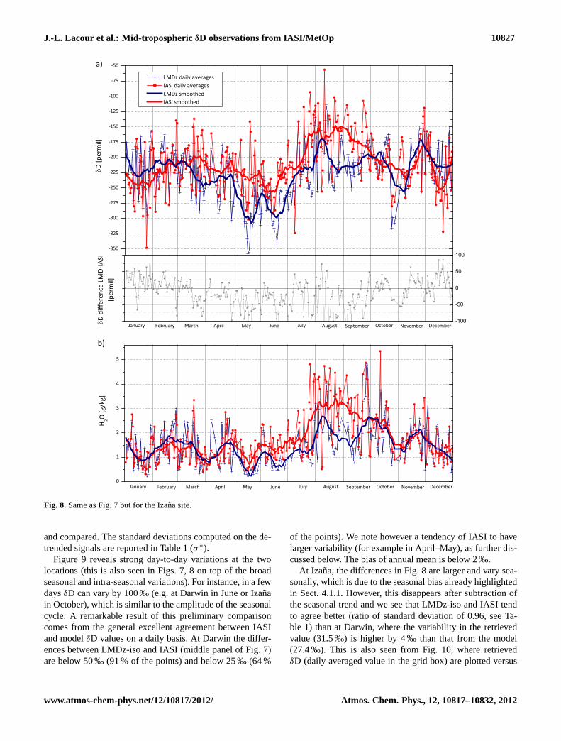
Izana, located in the northern Atlantic Ocean at subtropicallatitudes, is characteristic of a subsidence zone with a verydry climate. The time series for Izana is shown in Fig.8.A seasonal cycle is clearly identifiable with lowδD valuesin winter (min values of−250 ‰), and high values in sum-mer (max values of−150 ‰). The general agreement be-tween IASI and LMDz is good, but contrary to what we ob-served at Darwin, there are some noticeable differences inthe seasonal and intra-seasonal variations. In particular, theseasonality (difference between summer months and wintermonths) retrieved with IASI is larger than LMDz: in winterLMDz simulates higherδD values than IASI, and in summermodel simulations are lower. In the annual mean this trans-lates to a−15 ‰ bias of IASI compared to the model. Whilethese differences inδD could be due in part to the retrievals,we believe that they essentially come from the model, whichhas been shown before to underestimate theδD seasonal-ity in the subtropics (Risi et al., 2012b). Note that the dif-ferences do not apply to H2O (bottom panel of Fig.8), forwhich observations and simulations are in very good agree-ment during the winter months, but where IASI retrievals aresystematically higher than the model from May to the end ofSeptember. In June, the strong increase ofδD, followed by

www.atmos-chem-phys.net/12/10817/2012/ Atmos. Chem. Phys., 12, 10817–10832, 2012

10826 J.-L. Lacour et al.: Mid-tropospheric δD observations from IASI/MetOp

-275

-250

-225

-200

-175

-150

-125

-100

-75

LMDz daily averages IASI daily averages LMDz smoothed IASI smoothed

D [p

erm

il]

-100

-50

0

50

100

0

2

4

6

8

b)

H2O

[g/k

g]D

diff

eren

ce L

MD

-IA

SI[p

erm

il]

AugustMarch September October DecemberNovemberJune JulyFebruary April MayJanuary

a)

AugustMarch September October DecemberNovemberJune JulyFebruary April MayJanuary

Fig. 7.Time series at the Darwin site for the year 2010 for the 3–6 km layer.(a) Top pannel: IASIδD daily averages (red circles and line) arecompared to corresponding LMDz-iso simulations (blue crosses and line). A Savitzky-Golay smoothing filter has been applied (thick lines)to highlight seasonal and intra-seasonal pattern.(b) Same as(a) but for specific humidity in gkg−1.

the increase of water amount, probably indicates a decreasein subsidence.

4.1.2 Short term variability

Figure9 is provided in support of Figs.7 and8 to evaluatethe variability of the daily mean variations ofδD. Because adirect computation of the standard deviation of the daily aver-ages do not only reflect the day-to-day variability but also thevariability induced by the seasonal cycle, it is important to re-move the signal due to seasonal variations in order to analyze

the short term variability. This has been done by fitting a sea-sonal trend through the data points, which was subsequentlysubtracted. Fourier series, which integrate sum of sine andcosine functions, have been used to fit the seasonal behavior(dotted lines in Fig.9). As the model and the IASI time seriesexhibit slightly different seasonal behavior (see previous sec-tion), the fitted curve is different for each. TheδD time seriesat Izana and Darwin are plotted in Fig.9 with the fitted trendfor IASI (top panel) and LMDz (middle panel). The differ-ences for LMDz and IASI are plotted on the bottom panel

Atmos. Chem. Phys., 12, 10817–10832, 2012 www.atmos-chem-phys.net/12/10817/2012/

J.-L. Lacour et al.: Mid-tropospheric δD observations from IASI/MetOp 10827

-350

-325

-300

-275

-250

-225

-200

-175

-150

-125

-100

-75

-50

LMDz daily averages IASI daily averages LMDz smoothed IASI smoothed

D d

iffer

ence

LM

D-IA

SI[p

erm

il]H

2O [g

/kg]

D [p

erm

il]

0

1

2

3

4

5

b)

a)

AugustMarch September October DecemberNovemberJune JulyFebruary April MayJanuary

AugustMarch September October DecemberNovemberJune JulyFebruary April MayJanuary

-100

-50

0

50

100

Fig. 8.Same as Fig.7 but for the Izana site.

and compared. The standard deviations computed on the de-trended signals are reported in Table1 (σ ∗).

Figure 9 reveals strong day-to-day variations at the twolocations (this is also seen in Figs.7, 8 on top of the broadseasonal and intra-seasonal variations). For instance, in a fewdaysδD can vary by 100 ‰ (e.g. at Darwin in June or Izanain October), which is similar to the amplitude of the seasonalcycle. A remarkable result of this preliminary comparisoncomes from the general excellent agreement between IASIand modelδD values on a daily basis. At Darwin the differ-ences between LMDz-iso and IASI (middle panel of Fig.7)are below 50 ‰ (91 % of the points) and below 25 ‰ (64 %

of the points). We note however a tendency of IASI to havelarger variability (for example in April–May), as further dis-cussed below. The bias of annual mean is below 2 ‰.

At Izana, the differences in Fig.8 are larger and vary sea-sonally, which is due to the seasonal bias already highlightedin Sect.4.1.1. However, this disappears after subtraction ofthe seasonal trend and we see that LMDz-iso and IASI tendto agree better (ratio of standard deviation of 0.96, see Ta-ble 1) than at Darwin, where the variability in the retrievedvalue (31.5 ‰) is higher by 4 ‰ than that from the model(27.4 ‰). This is also seen from Fig.10, where retrievedδD (daily averaged value in the grid box) are plotted versus

www.atmos-chem-phys.net/12/10817/2012/ Atmos. Chem. Phys., 12, 10817–10832, 2012

10828 J.-L. Lacour et al.: Mid-tropospheric δD observations from IASI/MetOp

-250

-200

-150

-100

-300

-250

-200

-150

-100

-250

-200

-150

-100

-350

-300

-250

-200

-150

-100

-100

-50

0

50

100

-100

-50

0

50

100

IASI D Fitted trend

121110090807060502 040301

LMDz D Fitted trend

121110090807060502 0403

01

121110090807060502 040301

121110090807060502 040301

Izana 2010

121110090807060502 040301

Darwin 2010

LMDZ= 35 %o IASI = 37 %oLMDZ= 27 %o IASI = 32 %o

LMDz-Fitted trend IASI-Fitted trend

121110090807060502 040301

Fig. 9. δD time series at Darwin and Izana retrieved from IASI (top) and simulated by LMDz (middle). The dotted lines are fitted Fourierfunctions isolating the broad seasonal component of the variations. The bottom panels show the detrended time series obtained by subtractingthe Fourier functions from the raw data.

modelδD values. This figure also allows for a visualizationof the correlation pattern between the two different data sets.At Izana, we find a correlation coefficient of 0.5 (see also Ta-ble 1) when taking all observations into account. If we onlyconsider the IASI measurements for which the daily variabil-ity in the grid box is below 35 ‰, the correlation coefficientincreases to 0.64 with a slope still close to 1. At Darwin thiseffect is not observed; the slope of 1.22 indicates a larger am-plitude of the variations of IASI as compared to the model(similar indication than the standard deviations ratio). Thecorrelation coefficient is also relatively significant (0.55) here(Fig. 10and Table1).

4.2 Spatial variability along a latitudinal gradient

In addition to the temporal variations, we have examined theability of IASI to capture the spatial variability ofδD byconsidering a latitudinal band from−60◦ to 60◦. Figure11shows theδD and H2O latitudinal distributions representa-tive of the 3–6 km layer averaged on LMDz-iso grid boxes(from −30◦ to −25◦ in longitude above ocean surfaces) forthe first 15 days of January 2010. As expected, the retrievedδD are largest near the Equator (mean value of−140 ‰) anddecrease polewards to reach a minimum value of−350 ‰ at56◦ S (gradient of−210 ‰). Local maxima are observed inthe subtropics for both H2O andδD distributions but witha significant phase shift, withδD maxima being localized

at higher latitudes than H2O. This can be explained by thefact that at high and mid latitudes, isotopic composition fol-lows a Rayleigh type distillation, while at subtropical lati-tudes, the isotopic composition is sensitive to mixing pro-cesses, which will lead to an enrichment of the air parcel fora same water amount (Galewsky and Hurley, 2010). In thetropics, convection contributes to the depletion of air massesin the heavier isotopologues. These processes are responsiblefor the smoother behavior ofδD compared to H2O.

The retrieved values are in very good agreement withmodeled values for water vapour (correlation coefficient of0.90, ratio of standard deviations of 1.05 and a moist biasof 0.32 gkg−1). The observed variations are in phase withthe simulated ones. The only noticeable differences are thelower water concentration simulated by LMDz at the Equa-tor and the higher concentrations simulated in the southernsubtropics.

The comparison of theδD gradients is also very good ona global scale, with a correlation coefficient of 0.83. How-ever, large differences occur in the magnitude of the varia-tions with a ratio of standard deviations of 1.38 (LMDz hasa larger standard deviation (74.02 ‰) than IASI (53.46 ‰)).The timing of the variations is also quite good. The majordifferences occur in subtropical regions where LMDz sys-tematically simulates higherδD values than IASI and wherecorrespondence between the LMDz and IASI timing is not

Atmos. Chem. Phys., 12, 10817–10832, 2012 www.atmos-chem-phys.net/12/10817/2012/

J.-L. Lacour et al.: Mid-tropospheric δD observations from IASI/MetOp 10829

1

-350 -300 -250 -200 -150 -100 -50-350

-300

-250

-200

-150

-100

-50

-300 -250 -200 -150 -100 -50-300

-250

-200

-150

-100

-50

D IA

SI [

perm

il]

D LMDz [permil]

IASI = 0.9998 * LMD + 15.34 r = 0.5050 (N=324)

IASI = 1.0316 * LMD - 4.411 r = 0.6384 (N=231)

5.000

15.00

25.00

35.00

45.00

50.00

IASI= 1.22 * LMD + 39 r=0.5476 (N=267)

D

IAS

I [permil]

D LMDz [permil]

5.000

15.00

25.00

35.00

45.00

50.00

1

Fig. 10.Scatter plots of daily averagedδD IASI observations versus LMDz-iso simulations for Izana site (right) and Darwin site (left). Thecolor scale indicates the daily variability (1σ ) of IASI retrieved values in the model grid box. The dashed and the dashed-dotted lines arereduced major axis regressions on all points (dashed green lines) and, for Izana, on points with a 1σ variability in the model grid box lowerthan 35. In the case of Izana, there is clear increase of the correlation coefficient (from 0.5 to 0.64) when considering onlyδD averages witha certain variability threshold (averages with a daily variability inferior to 35 ‰, dashed-dotted violet line). The line equations, the correlationcoefficient and the number of coincident values are given above the figures.

-350 -300 -250 -200 -150 -100-60

-45

-30

-15

0

15

30

45

60-350 -300 -250 -200 -150 -100

IASI 3-6 km H2O

LMDz 3-6 km H2O

IASI 3-6 km D LMDz 3-6 km D

-25-30-25-30Longitude Longitude

Lat

itude

Lat

itude

D [permil]

0.0 0.5 1.0 1.5 2.0 2.5 3.0 3.5 4.0 4.5-60

-45

-30

-15

0

15

30

45

600.0 0.5 1.0 1.5 2.0 2.5 3.0 3.5 4.0 4.5

-350

-250

-200

-150

4.0

2.0

0.5

1.5

3.0

1.0

2.5

3.5

[g/kg]

H2O [g/kg]

[permil]

-300

Fig. 11.Latitudinal distribution ofδD (left) with δD a priori (gray dashed-dotted line) and H2O (right) retrieved with IASI (red) and simulatedby LMDz-iso (blue).δD retrievals, representative of the 3–6 km layer, have been averaged on the first 15 days of January 2010 and on theLMDz-iso grid boxes. The corresponding spatial distributions of IASI retrievals are mapped besides the latitudinal gradients.

www.atmos-chem-phys.net/12/10817/2012/ Atmos. Chem. Phys., 12, 10817–10832, 2012

10830 J.-L. Lacour et al.: Mid-tropospheric δD observations from IASI/MetOp

good. Noticeable differences also appear between 45◦ and60◦ where LMDz values are much lower than the retrievedvalues, differences reaching 100 ‰ around 54◦. In additionto the underestimation of the seasonality at subtropical lati-tudes,Risi et al.(2012b) have identified an underestimationof the latitudinal gradient (zonal annual mean) and in partic-ular a pronounced high bias inδD at subtropical latitudes asrobust features of the model. While we do not observe theunderestimation of latitudinal gradient by LMDz, our com-parison tends to confirm a misrepresentation of the processesaffectingδD in the subtropics. A detailed study of the IASIto model differences is beyond the scope of the present paperand will be the subject of forthcoming analyses.

5 Conclusions

We have described a new joint retrieval methodology forH2O and HDO from IASI radiances spectra. Based on op-timal estimation, the method is different from our previouswork in that it constrains the retrievals by explicitly intro-ducing correlations in the concentrations of the two speciesinside the a priori covariance matrixSa. This matrix was builtfrom a global set of daily vertical profiles from the LMDz-iso GCM representative of the whole year. It therefore showslarge variability around the a priori (the average profile ofH2O and HDO). TheSa matrix was slightly modified to de-crease the modeled correlations between the two species. Thespectral range for the retrievals was set to 1193 to 1253 cm−1

with a gap between 1223 and 1251 cm−1. With these settings,we show that IASI provides maximum sensitivity simultane-ously to HDO and H2O in the free troposphere with errors onthe retrievedδD vertical profiles lower than 40 ‰ between 2and 5 km. For an individual retrieval, the standard deviationonδD in the 3–6 km layer is 38 ‰ and was shown to be dom-inated by the measurement noise.

The seasonal variability of IASI retrievedδD values wasexamined at two locations for the year 2010, and comparedto that of the LMDz-iso model. We found a general excellentagreement in the magnitude of the seasonal pattern, althoughlocal differences exist. While at Izana a clear seasonal biashas been identified (overall bias of 15 ‰), the bias at Darwinis insignificant (< 2 ‰). Beyond the seasonal cycle, we havedemonstrated the good performance of IASI to capture short-term variations ofδD (e.g. day-to-day variations) despite sig-nificant differences in the amplitude of variations estimatedbetween the model and the measurements at Darwin. It isworthwhile mentioning that IASI is currently the only satel-lite sounder that allows monitoringδD on a daily basis. Fi-nally, we have investigated the performance of the retrievalsby analyzing theδD results for a 5◦ wide longitude band from−60◦ S to 60◦ N for the first 15 days of January. We showthat the retrieved values are in very good agreement with themodel (correlation coefficient of 0.83), even though notice-able differences occur. These are a significant deviation be-

tween LMDz and IASI at subtropical latitudes and also lowerδD values simulated beyond the 45◦ latitudes. While differ-ences highlighted in this study could still be due to retrievalissues, they confirm previously documented shortcomings ofthe model.

More generally, results presented here highlight further theexceptional potential of IASI to contribute to the understand-ing of hydrological processes.

Acknowledgements.IASI has been developed and built under theresponsibility of the Centre National d’Etudes Spatiales (CNES,France). It is flown onboard the MetOp satellites as part of theEUMETSAT Polar System. The IASI L1 data are received throughthe EUMETCast near real time data distribution service. Theresearch in Belgium was funded by the “Communaute Francaise deBelgique – Actions de Recherche Concertees”, the Fonds Nationalde la Recherche Scientifique (FRS-FNRS F.4511.08), the BelgianScience Policy Office and the European Space Agency (ESA-Prodex C90-327). L. Clarisse and P.-F. Coheur are respectivelyPostdoctoral Researcher (Charge de Recherches) and ResearchAssociate (Chercheur Qualifie) with F.R.S.-FNRS. C. Clerbaux isgrateful to CNES for scientific collaboration and financial support.The authors would like to thank J. Worden and M. Schneider fortheir comments during the review process which greatly improvedthis manuscript.

Edited by: G. Stiller

References

Berkelhammer, M., Risi, C., Kurita, N., and Noone, D. C.: Themoisture source sequence for the Madden-Julian Oscillation asderived from satellite retrievals of HDO and H2O, J. Geophys.Res., 117, D03106,doi:10.1029/2011JD016803, 2012.

Bony, S., Colman, R., Kattsov, V., Allan, R., Bretherton, C.,Dufresne, J., Hall, A., Hallegatte, S., Holland, M., Ingram, V.,Randall, D., Soden, B., Tselioudis, G., and Webb, M.: How WellDo We Understand and Evaluate Climate Change Feedback Pro-cesses?, J. Climate, 19, 3445–3482, 2006.

Clerbaux, C., Boynard, A., Clarisse, L., George, M., Hadji-Lazaro,J., Herbin, H., Hurtmans, D., Pommier, M., Razavi, A., Turquety,S., Wespes, C., and Coheur, P. F.: Monitoring of atmosphericcomposition using the thermal infrared IASI/MetOp sounder, At-mos. Chem. Phys., 9, 6041–6054,doi:10.5194/acp-9-6041-2009,2009.

Craig, H.: Isotopic Variations in Meteoric Waters, Science, 133,1702–1703,doi:10.1126/science.133.3465.1702, 1961.

Ehhalt, D. H.: Vertical profiles of HTO, HDO, and H2O in theTroposphere, NCAR-TN/STR-100, Natl. Cent. for Atmos. Res.,Boulder, Colo., 1974.

Frankenberg, C., Yoshimura, K., Warneke, T., Aben, I., Butz,A., Deutscher, N., Griffith, D., Hase, F., Notholt, J., Schnei-der, M., Schrijver, H., and Rockmann, T.: Dynamic Pro-cesses Governing Lower-Tropospheric HDO/H2O Ratios as Ob-served from Space and Ground, Science, 325, 1374–1377,doi:10.1126/science.1173791, 2009.

Atmos. Chem. Phys., 12, 10817–10832, 2012 www.atmos-chem-phys.net/12/10817/2012/

J.-L. Lacour et al.: Mid-tropospheric δD observations from IASI/MetOp 10831

Frierson, D. M. W.: The Dynamics of Idealized ConvectionSchemes and Their Effect on the Zonally Averaged Tropical Cir-culation, J. Atmos. Sci., 64, 1959–1976,doi:10.1175/JAS3935.1,2007.

Galewsky, J. and Hurley, J. V.: An advection-condensation modelfor subtropical water vapor isotopic ratios, J. Geophys. Res., 115,D16116,doi:10.1029/2009JD013651, 2010.

Galewsky, J., Strong, M., and Sharp, Z. D.: Measurements of watervapor D/H ratios from Mauna Kea, Hawaii, and implications forsubtropical humidity dynamics, Geophys. Res. Lett., 34, L22808,doi:10.1029/2007GL031330, 2007.

Galewsky, J., Rella, C., Sharp, Z., Samuels, K., and Ward, D.: Sur-face measurements of upper tropospheric water vapor isotopiccomposition on the Chajnantor Plateau, Chile, Geophys. Res.Lett., 38, L17803,doi:10.1029/2011GL048557, 2011.

Herbin, H., Hurtmans, D., Clerbaux, C., Clarisse, L., and Co-heur, P.-F.: H16

2 O and HDO measurements with IASI/MetOp,Atmos. Chem. Phys., 9, 9267–9290,doi:10.5194/acpd-9-9267-2009, 2009.

Hilton, F., Armante, R., August, T., Barnet, C., Bouchard, A.,Camy-Peyret, C., Capelle, V., Clarisse, L., Clerbaux, C., Co-heur, P.-F., Collard, A., Crevoisier, C., Dufour, G., Edwards, D.,Faijan, F., Fourrie, N., Gambacorta, A., Goldberg, M., Guidard,V., Hurtmans, D., Illingworth, S., Jacquinet-Husson, N., Kerzen-macher, T., Klaes, D., Lavanant, L., Masiello, G., Matricardi,M., McNally, A., Newman, S., Pavelin, E., Payan, S., Pequignot,E., Peyridieu, S., Phulpin, T., Remedios, J., Schlussel, P., Serio,C., Strow, L., Stubenrauch, C., Taylor, J., Tobin, D., Wolf, W.,and Zhou, D.: Hyperspectral Earth Observation from IASI: FiveYears of Accomplishments, B. Am. Meteor. Soc., 93, 347–370,doi:10.1175/BAMS-D-11-00027.1, 2012.

Hurtmans, D., Coheur, P.-F., Wespes, C., Clarisse, L., Scharf,O., Clerbaux, C., Hadji-Lazaro, J., George, M., and Tur-quety, S.: FORLI radiative transfer and retrieval codefor IASI, J. Quant. Spectrosc. Ra., 113, 1391–1408,doi:10.1016/j.jqsrt.2012.02.036, 2012.

Johnson, L. R., Sharp, Z. D., Galewsky, J., Strong, M., Van Pelt,A. D., Dong, F., and Noone, D.: Hydrogen isotope correction forlaser instrument measurement bias at low water vapor concentra-tion using conventional isotope analyses: application to measure-ments from Mauna Loa Observatory, Hawaii, Rapid Commun.Mass Sp., 25, 608–616,doi:10.1002/rcm.4894, 2011.

Kang, S. M., Held, I. M., Frierson, D. M. W., and Zhao, M.: TheResponse of the ITCZ to Extratropical Thermal Forcing: Ideal-ized Slab-Ocean Experiments with a GCM, J. Climate, 21, 3521–3532,doi:10.1175/2007JCLI2146.1, 2008.

Kiehl, J. T. and Trenberth, K. E.: Earth’s Annual Global MeanEnergy Budget, Bull. Amer. Meteor. Soc., 78, 197–208,doi:10.1175/1520-0477(1997)078<0197:EAGMEB>2.0.CO;2,1997.

Kurita, N., Noone, D., Risi, C., Schmidt, G. A., Yamada, H., andYoneyama, K.: Intraseasonal isotopic variation associated withthe Madden-Julian Oscillation, J. Geophys. Res., 116, D24101,doi:10.1029/2010JD015209, 2011.

Lee, J., Worden, J., Noone, D., Bowman, K., Eldering, A.,LeGrande, A., Li, J.-L. F., Schmidt, G., and Sodemann, H.: Re-lating tropical ocean clouds to moist processes using water va-por isotope measurements, Atmos. Chem. Phys., 11, 741–752,doi:10.5194/acp-11-741-2011, 2011.

Noone, D., Galewsky, J., Sharp, Z. D., Worden, J., Barnes, J., Baer,D., Bailey, A., Brown, D. P., Christensen, L., Crosson, E., Dong,F., Hurley, J. V., Johnson, L. R., Strong, M., Toohey, D., Van Pelt,A., and Wright, J. S.: Properties of air mass mixing and humidityin the subtropics from measurements of the D/H isotope ratio ofwater vapor at the Mauna Loa Observatory, J. Geophys. Res.,116, D22113,doi:10.1029/2011JD015773, 2011.

Pougatchev, N., August, T., Calbet, X., Hultberg, T., Oduleye,O., Schlussel, P., Stiller, B., Germain, K. S., and Bingham,G.: IASI temperature and water vapor retrievals – error as-sessment and validation, Atmos. Chem. Phys., 9, 7971–7989,doi:10.5194/acpd-9-7971-2009, 2009.

Randall, D. A., Harshvardhan, Dazlich, D. A., and Corsetti,T. G.: Interactions among Radiation, Convection, andLarge-Scale Dynamics in a General Circulation Model,J. Atmos. Sci., 46, 1943–1970, doi:10.1175/1520-0469(1989)046<1943:IARCAL>2.0.CO;2, 1989.

Risi, C., Bony, S., Vimeux, F., Frankenberg, C., Noone, D., andWorden, J.: Understanding the Sahelian water budget through theisotopic composition of water vapor and precipitation, J. Geo-phys. Res., 115, D24110,doi:10.1029/2010JD014690, 2010a.

Risi, C., Bony, S., Vimeux, F., and Jouzel, J.: Water-stable isotopesin the LMDZ4 general circulation model: Model evaluation forpresent-day and past climates and applications to climatic in-terpretations of tropical isotopic records, J. Geophys. Res., 115,D12118,doi:10.1029/2009JD013255, 2010b.

Risi, C., Noone, D., Worden, J., Frankenberg, C., Stiller, G., Kiefer,M., Funke, B., Walker, K., Bernath, P., Schneider, M., Bony, S.,Lee, J., Brown, D., and Sturm, C.: Process-evaluation of tropo-spheric humidity simulated by general circulation models us-ing water vapor isotopic observations: 2. Using isotopic diag-nostics to understand the mid and upper tropospheric moist biasin the tropics and subtropics, J. Geophys. Res., 117, D05304,doi:10.1029/2011JD016623, 2012a.

Risi, C., Noone, D., Worden, J., Frankenberg, C., Stiller, G.,Kiefer, M., Funke, B., Walker, K., Bernath, P., Schneider, M.,Wunch, D., Sherlock, V., Deutscher, N., Griffith, D., Wennberg,P. O., Strong, K., Smale, D., Mahieu, E., Barthlott, S., Hase,F., Garcıa, O., Notholt, J., Warneke, T., Toon, G., Sayres, D.,Bony, S., Lee, J., Brown, D., Uemura, R., and Sturm, C.: Process-evaluation of tropospheric humidity simulated by general cir-culation models using water vapor isotopologues: 1. Compar-ison between models and observations, J. Geophys. Res., 117,D05303,doi:10.1029/2011JD016621, 2012b.

Rodgers, C. D.: Inverse methods for atmospheric sounding: theoryand practise, World Scientific, 2000.

Rothman, L. S., Barbe, A., Chris Benner, D., Brown, L. R., Camy-Peyret, C., Carleer, M. R., Chance, K., Clerbaux, C., Dana, V.,Devi, V. M., Fayt, A., Flaud, J. M., Gamache, R. R., Goldman,A., Jacquemart, D., Jucks, K. W., Lafferty, W. J., Mandin, J. Y.,Massie, S. T., Nemtchinov, V., Newnham, D. A., Perrin, A., Rins-land, C. P., Schroeder, J., Smith, K. M., Smith, M. A. H., Tang,K., Toth, R. A., Vander Auwera, J., Varanasi, P., and Yoshino,K.: The HITRAN molecular spectroscopic database: edition of2000 including updates through 2001, J. Quant. Spectrosc. Ra.,82, 5–44, 2003.

Schlussel, P., Hultberg, T. H., Phillips, P. L., August, T., and Calbet,X.: The operational IASI Level 2 processor, Adv. Space Res., 36,982–988, 2005.

www.atmos-chem-phys.net/12/10817/2012/ Atmos. Chem. Phys., 12, 10817–10832, 2012

10832 J.-L. Lacour et al.: Mid-tropospheric δD observations from IASI/MetOp

Schmidt, G. A., Ruedy, R. A., Miller, R. L., and Lacis, A. A.: At-tribution of the present-day total greenhouse effect, J. Geophys.Res., 115, D20106,doi:10.1029/2010JD014287, 2010.

Schneider, M. and Hase, F.: Optimal estimation of troposphericH2O and deltaD with IASI/METOP, Atmos. Chem. Phys., 11,16107–16146,doi:10.5194/acpd-11-16107-2011, 2011.

Schneider, M., Hase, F., and Blumenstock, T.: Ground-based re-mote sensing of HDO/H2O ratio profiles: introduction and vali-dation of an innovative retrieval approach, Atmos. Chem. Phys.,6, 4705–4722,doi:10.5194/acp-6-4705-2006, 2006.

Schneider, M., Yoshimura, K., Hase, F., and Blumenstock, T.: Theground-based FTIR network’s potential for investigating the at-mospheric water cycle, Atmos. Chem. Phys., 10, 3427–3442,doi:10.5194/acp-10-3427-2010, 2010a.

Schneider, T., O’Gorman, P. A., and Levine, X. J.: Water vapor andthe dynamics of climate changes, Rev. Geophys., 48, RG3001,doi:10.1029/2009RG000302, 2010b.

Schneider, M., Barthlott, S., Hase, F., Gonzalez, Y., Yoshimura,K., Garcıa, O. E., Sepulveda, E., Gomez-Pelaez, A., Gisi, M.,Kohlhepp, R., Dohe, S., Blumenstock, T., Strong, K., Weaver,D., Palm, M., Deutscher, N. M., Warneke, T., Notholt, J., Leje-une, B., Demoulin, P., Jones, N., Griffith, D. W. T., Smale, D.,and Robinson, J.: Ground-based remote sensing of troposphericwater vapour isotopologues within the project MUSICA, Atmos.Meas. Tech. Discuss., 5, 5357–5418,doi:10.5194/amtd-5-5357-2012, 2012.

Sherwood, S. C., Roca, R., Weckwerth, T. M., and Andronova,N. G.: Tropospheric water vapor, convection, and climate, Rev.Geophys., 48, RG2001,doi:10.1029/2009RG000301, 2010.

Soden, B. J. and Held, I. M.: An Assessment of Climate Feedbacksin Coupled Ocean Atmosphere Models, J. Climate, 19, 3354–3360,doi:10.1175/JCLI3799.1, 2006.

Strong, M., Sharp, Z. D., and Gutzler, D. S.: Diagnosing moisturetransport using D/H ratios of water vapor, Geophys. Res. Lett.,34, L03404,doi:10.1029/2006GL028307, 2007.

Taylor, K. E.: Summarizing multiple aspects of model perfor-mance in a single diagram, J. Geophys. Res., 106, 7183–7192,doi:10.1029/2000JD900719, 2001.

Toth, R. A.: HDO and D2O Low Pressure, Long Path Spectra in the600–3100 cm−1 Region: I. HDO Line Positions and Strengths,J. Molec. Spectrosc., 195, 73–97, 1999.

Worden, J., Bowman, K., Noone, D., Beer, R., Clough, S., Elder-ing, A., Fisher, B., Goldman, A., Gunson, M., Herman, R., Ku-lawik, S. S., Lampel, M., Luo, M., Osterman, G., Rinsland, C.,Rodgers, C., Sander, S., Shephard, M., and Worden, H.: Tropo-spheric Emission Spectrometer observations of the troposphericHDO/H2O ratio: Estimation approach and characterization, J.Geophys. Res., 111, D16309,doi:10.1029/2005JD006606, 2006.

Worden, J., Noone, D., and Bowman, K.: Importance of rain evap-oration and continental convection in the tropical water cycle,Nature, 445, 528–532,doi:10.1038/nature05508, 2007.

Worden, J., Kulawik, S., Frankenberg, C., Payne, V., Bowman, K.,Cady-Peirara, K., Wecht, K., Lee, J.-E., and Noone, D.: Pro-files of CH4, HDO, H2O, and N2O with improved lower tro-pospheric vertical resolution from Aura TES radiances, Atmos.Meas. Tech., 5, 397–411,doi:10.5194/amt-5-397-2012, 2012.

Yoshimura, K., Frankenberg, C., Lee, J., Kanamitsu, M., Worden,J., and Rockmann, T.: Comparison of an isotopic atmosphericgeneral circulation model with new quasi-global satellite mea-surements of water vapor isotopologues, J. Geophys. Res., 116,D19118,doi:10.1029/2011JD016035, 2011.

Zhang, R., Kang, S. M., and Held, I. M.: Sensitivity of ClimateChange Induced by the Weakening of the Atlantic MeridionalOverturning Circulation to Cloud Feedback, J. Climate, 23, 378–389,doi:10.1175/2009JCLI3118.1, 2010.

Zhou, D., Larar, A., Liu, X., Smith, W., Strow, L., Yang, P.,Schlussel, P., and Calbet, X.: Global Land Surface Emis-sivity Retrieved From Satellite Ultraspectral IR Measure-ments, IEEE Trans. Geosci. Remote Sens, 49, 1277–1290,doi:10.1109/TGRS.2010.2051036, 2011.

Atmos. Chem. Phys., 12, 10817–10832, 2012 www.atmos-chem-phys.net/12/10817/2012/