Embed Size (px)
Citation preview

Adv Data Anal Classif (2016) 10:139–154DOI 10.1007/s11634-016-0234-1
REGULAR ARTICLE
Micro–macro multilevel latent class modelswith multiple discrete individual-level variables
Margot Bennink1 · Marcel A. Croon1 ·Brigitte Kroon1 · Jeroen K. Vermunt1
Received: 7 May 2014 / Revised: 5 January 2016 / Accepted: 19 January 2016 /Published online: 16 February 2016© The Author(s) 2016. This article is published with open access at Springerlink.com
Abstract An existing micro–macro method for a single individual-level variable isextended to the multivariate situation by presenting two multilevel latent class modelsin which multiple discrete individual-level variables are used to explain a group-leveloutcome. As in the univariate case, the individual-level data are summarized at thegroup-level by constructing a discrete latent variable at the group level and this group-level latent variable is used as a predictor for the group-level outcome. In the firstextension, that is referred to as theDirectmodel, themultiple individual-level variablesare directly used as indicators for the group-level latent variable. In the second exten-sion, referred to as the Indirect model, the multiple individual-level variables are usedto construct an individual-level latent variable that is used as an indicator for the group-level latent variable. This implies that the individual-level variables are used indirectlyat the group-level. Thewithin- and between components of the (co)varn the individual-level variables are independent in the Direct model, but dependent in the Indirectmodel. Both models are discussed and illustrated with an empirical data example.
Keywords Latent class analysis · Micro-macro analysis · Multilevel analysis ·Discrete data
B Margot [email protected]; [email protected]
Marcel A. [email protected]
Brigitte [email protected]
Jeroen K. [email protected]
1 Tilburg University, P.O. Box 90153, 5000 LE Tilburg, The Netherlands
123
140 M. Bennink et al.
1 Introduction
In many research areas, data are collected on individuals (micro-level units) that arenested within groups (macro-level units) (Goldstein 2011). For example, data can becollected on children nested in schools, on employees nested in organizations, or onfamily members nested in families. The variables involved may be either measured atthe individual level or at the level of the groups. Following, Snijders andBosker (2012),one can distinguish between macro–micro and micro–macro situations. In a macro–micro situation, the outcome or dependent variable is measured at the individual level,while in a micro–macro situation, the outcome variable is measured at the group level.The current article focuses on the latter type of multilevel analysis that is neededwhen, for example, characteristics of household members are related to householdownership of financial products, or when psychological characteristics of employeesare related to organizational performance outcomes. Furthermore, attention is focusedon micro–macro analysis for discrete data.
In micro–macro analysis, the individual-level data need to be aggregated to thegroup level, so the aggregated scores can be related to the group-level outcome. Whena group mean or mode is used for aggregation, measurement and sampling error in theindividual scores is not accounted for and Croon and van Veldhoven (2007) showedthat this neglect of random fluctuation in the individual scores causes bias in theestimates of the group-level parameters. Moreover, this type of aggregation wipes outall individual differences within the groups and it is well known that the variabilityof the group means and modes not only represents between-group variation but alsopartly reflects within-group variation. Therefore, the analysis of observations frommicro–macro designs requires an appropriate methodology that takes into accountthe measurement and sampling error of the individual scores and neatly separates thebetween- and within-group association among the variables (Preacher et al. 2010).
Such techniques have been developed by using a group-level latent variable for theaggregation. For continuous data, Croon and van Veldhoven (2007) provide a basicexample of this methodology. The scores of the individuals i from group j on anexplanatory variable Zi j are interpreted as exchangeable indicators of an unobservedgroup score on the continuous latent group-level variable ζ j . Furthermore, the latentvariable is treated as a group-level mediating variable between a group-level predictorX j and a group-level outcome Y j . Figure 1 represents this model graphically. Anytheory in which a group-level intervention is not only expected to influence a group-level (performance) measure directly, but also indirectly through a characteristic ofthe group members, can be tested with this model.
The model belongs to the general framework of generalized latent variable mod-els described by Skrondal and Rabe-Hesketh (2004) and can also be formulated forcategorical data (Bennink et al. 2013), by using a latent class model instead of afactor–analytic model that was used for continuous variables. The latent variable ζ jthen becomes a categorical variable with C categories, c = 1, . . . ,C . The scores Zi j
of the I j individuals in group j (collected in the vector Z j ) are treated as ‘unreliable’indicators of the group score ζ j . For an arbitrary group j , the relevant conditionalprobability distribution for the manifest variables Y j and Z j given X j is:
123

Micro–macro multilevel latent class 141
Fig. 1 Micro–macro latentvariable model with onemicro-level variable
Yj
ζj
Zij
Xj
individual level
group level
P(Y j , Z j |X j ) =C∑
c=1
P(Y j , ζ j = c|X j )P(Z j |ζ j = c). (1)
The terms on the right hand side of the equation are the between and within part thatcan be further decomposed as
P(Y j , ζ j = c|X j ) = P(ζ j = c|X j )P(Y j |X j , ζ j = c), (2)
and
P(Z j |ζ j = c) =I j∏
i=1
P(Zi j |ζ j = c). (3)
Since in the social and behavioral sciences it is very common to use multipleindividual-level variables instead of only a single one, in the present article two mul-tilevel latent class models are presented that extend the univariate case to the situationwith multiple Zi j -variables. As in the existing method, the Zi j -variables are summa-rized by a single discrete latent variable at the group level (ζ j ). In the first model,that is referred to as the Direct model, the Zi j -variables are directly used as indica-tors for ζ j , while in the second model, that is referred to as the Indirect model, thisis done indirectly through an individual-level latent variable (ηi j ). The Direct modelcan, for example, be used to construct a latent classification of households based onthe age, gender and educational level of the household members to predict householdownership of financial products. In other words, individual-level information can besummarized at the group-level by constructing a group-level typology based on theindividual-level variables. The Indirect model can, for example, be usedwhenmultipleindividual-level items on the satisfaction of employees with respect to their relation-ships at work are used to construct the individual-level latent variable ηi j that is used asan indicator for ζ j to predict organizational performance measures, such as the level oforganizational conflicts. The Indirect model makes it possible to allow groups to differwith respect to the proportion of individuals that belong to the various individual-levellatent classes. In the remaining article, both methods and their estimation proceduresare discussed and applied to empirical data examples.
123
142 M. Bennink et al.
Yj
ζj
Z2ij
Xj
ZKijZ1ij
ηij
...
Xj Yj
ζj
...Z1ij Z2ij ZKij
Direct ass model Direct lv model
individual level
group level
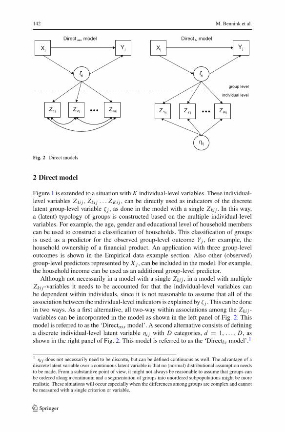
Fig. 2 Direct models
2 Direct model
Figure 1 is extended to a situation with K individual-level variables. These individual-level variables Z1i j , Zki j . . . ZKi j , can be directly used as indicators of the discretelatent group-level variable ζ j , as done in the model with a single Zki j . In this way,a (latent) typology of groups is constructed based on the multiple individual-levelvariables. For example, the age, gender and educational level of household memberscan be used to construct a classification of households. This classification of groupsis used as a predictor for the observed group-level outcome Y j , for example, thehousehold ownership of a financial product. An application with three group-leveloutcomes is shown in the Empirical data example section. Also other (observed)group-level predictors represented by X j , can be included in the model. For example,the household income can be used as an additional group-level predictor.
Although not necessarily in a model with a single Zki j , in a model with multipleZki j -variables it needs to be accounted for that the individual-level variables canbe dependent within individuals, since it is not reasonable to assume that all of theassociation between the individual-level indicators is explained by ζ j . This can be donein two ways. As a first alternative, all two-way within associations among the Zki j -variables can be incorporated in the model as shown in the left panel of Fig. 2. Thismodel is referred to as the ‘Directass model’. A second alternative consists of defininga discrete individual-level latent variable ηi j with D categories, d = 1, . . . , D, asshown in the right panel of Fig. 2. This model is referred to as the ‘Directlv model’.1
1 ηi j does not necessarily need to be discrete, but can be defined continuous as well. The advantage of adiscrete latent variable over a continuous latent variable is that no (normal) distributional assumption needsto be made. From a substantive point of view, it might not always be reasonable to assume that groups canbe ordered along a continuum and a segmentation of groups into unordered subpopulations might be morerealistic. These situations will occur especially when the differences among groups are complex and cannotbe measured with a single criterion or variable.
123

Micro–macro multilevel latent class 143
As in Eq. (1), the probability distribution of an arbitrary group j contains a betweenand a within term. For both models the between part is still represented by Eq. (2), butthey differ with respect to the within part. For the Directass model, the within part is
P(Z j |ζ j = c) =I j∏
i=1
P(Z1i j , . . . Zki j , . . . ZKi j |ζ j = c), (4)
whereas for the Directlv model, the within part is
P(Z j |ζ j = c) =I j∏
i=1
D∑
d=1
P(ηi j = d)
K∏
k=1
P(Zki j |ζ j = c, ηi j = d). (5)
The group members are used as exchangeable indicators, this implies thatP(Z1i j , Zki j , . . . ZKi j |ζ j = c) in the Directass model and P(Zki j |ζ j = c, ηi j = d)
in the Directlv model, are identical for all individuals. In the Directass model, thereis by definition local dependency among the indicators given ζ j , but in the Directlvmodel, the indicators are locally independent given ηi j and ζ j . It is also important tonote is that ηi j and ζ j are assumed to be independent.
3 Indirect model
When the K individual-level variables were intended in the first place to measure anindividual-level construct, the relationship between the group-level latent variable andthe individual-level items can be specified indirectly rather than directly. For example,suppose that the satisfaction of employees with their relationships at work is measuredby three indicators: (1) their satisfaction with the relation with their supervisor, (2) thesatisfaction with their relation with other coworkers, and (3) the degree in which theyexperience a family culture at their working environment. These three Zki j -variablesmay be treated as indicators of an underlying latent construct at the individual-level(ηi j ). In the current article ηi j is a discrete variable with D categories, d = 1, . . . , D.2
Since there may exist group differences on ηi j , a group-level latent variable (ζ j ) maybe invoked to represent these between-group differences on ηi j .
This model containing a single group-level outcome Y j is graphically shown inFig. 3 and referred to as the ‘Indirect model’. We will show an example with twogroup-level outcomes in the Empirical data examples section.
Referring to the formal general description in Eq. (1), the between part of thismodelis represented again by Eq. (2), but the within part is now:
P(Z j |ζ j = c) =I j∏
i=1
D∑
d=1
P(ηi j = d|ζ j = c)K∏
k=1
P(Zki j |ηi j = d). (6)
The groupmembers are again treated as exchangeable, so that P(Zki j |ηi j = d) has thesame form for all individuals. The individual-level variables are locally independent
2 Varriale and Vermunt (2012) proposed a similar model with a continuous ηi j and no group-level outcome.
123

144 M. Bennink et al.
Fig. 3 Indirect modelYj
ζj
Z2ij
Xj
ZKijZ1ij
ηij
...
individual level
group level
givenηi j and the two latent variables are dependent since the distribution ofηi j dependson ζ j . In this model there is no immediate need to allow for residual association amongthe individual indicators since ηi j is assumed to account for all of the associations thatexist among the indicators.
4 Estimation, identification, and model selection
The micro–macro models presented above are extended versions of the multilevellatent class model proposed by Vermunt (2003). The extension involves that, in addi-tion to having discrete latent variables at two levels, these models contain an outcomevariable at the group level. Vermunt (2003) showed how to obtain maximum likeli-hood estimates for multilevel latent class models using an EM algorithm, and a verysimilar procedure can be used here. The log-likelihood to be maximized equals:
log L =J∑
j=1
log P(Y j , Z j |X j )
=J∑
j=1
log
[C∑
c=1
P(ζ j = c|X j )P(Y j |X j , ζ j = c)
I j∏
i=1
D∑
d=1
P(ηi j = d|ζ j = c)P(Zi j |ζ j = c, ηi j = d)
⎤
⎦ , (7)
while the complete data likelihood equals:
Lcomp =J∏
j=1
P(Y j , Z j , X j , ζ j , η j )
=J∏
j=1
⎡
⎣P(X j )P(ζ j |X j )P(Y j |X j , ζ j )
I j∏
i=1
P(ηi j |ζ j )P(Zi j |ζ j , ηi j )⎤
⎦. (8)
123

Micro–macro multilevel latent class 145
The expected complete-data log-likelihood, which is computed in the E-step andmaximized in the M-step, has the following form:
E(log Lcomp) =J∑
j=1
C∑
c=1
πcj log P(ζ j = c|X j )
+J∑
j=1
C∑
c=1
πcj log P(Y j |X j , ζ j= c)
+J∑
j=1
I j∑
i=1
C∑
c=1
D∑
d=1
πcdi j log P(ηi j = d|ζ j = c)
+J∑
j=1
I j∑
i=1
C∑
c=1
D∑
d=1
πcdi j log P(Zi j |ζ j = c, ηi j = d). (9)
Here, πcj and πcd
i j denote the posterior class membership probabilities P(ζ j =c|Y j , Z j , X j ) and P(ζ j = c, ηi j = d|Y j ,Z j , X j ), respectively. These posteriorprobabilities can be obtained in an efficient manner using an upward–downward algo-rithm. In the upward step we obtain πk
j and in the downward step we obtain πcdi j
as πcj P(ηi j = d|ζ j = c,Y j , Zi j , X j ). This algorithm is implemented in the Latent
GOLD program (Vermunt and Magidson 2013) that we used for parameter estimationin the empirical examples presented in the next section.
Since the four sets of model probabilities are parametrized using logit models, theM step involves updating the estimates of a set of logistic parameters in the usual way.Note that the three special cases of the micro–macro model are all restricted versionsof the general model for which we defined the expected complete-data log-likelihood.The Directass model does not contain a lower-level latent variable, which can bespecified by setting D = 1. In this model, the joint distribution of Zi j is modeledwith a multivariate logistic model containing the two-variable associations betweenthe responses. In the Directlv model and the Indirect model, we assume responses Zki j
to be locally independent, meaning that the associations between the responses arefixed to zero. Moreover, in the former Zki j is assumed to be independent of ζ j givenP(Z1i j , . . . Zki j , . . . ZKi j and in the latter ηi j is assumed to be independent of ζ j ,which are restrictions that can be obtained by fixing the logistic parameters concernedto zero.
As regards the identifiability of the models proposed in this article, similar con-ditions apply as for regular latent class models. There is no sufficient and necessarycondition available to unassailable determine the identifiability of complex latent classmodels. A sufficient, but not necessary, condition for identification is that both theindividual- and the group-level part of the model are identified latent class models(Vermunt 2005). For the individual-level model this means that we need at least threeZki j -variables (K ≥ 3), whereas for the group-level model this means that mostgroups should have at least three individuals (I j ≥ 3). However, also when theseconditions are not fulfilled, the micro-macro model concerned may be identified. For
123
146 M. Bennink et al.
example, the Directass model, which contains only a group-level latent variable, isalso identified with two individuals per group when K ≥ 2, and the Indirect modelis also identified with K = 2 and I j ≥ 3. A formal way to check identification is todetermine the rank of the Jacobian matrix and the empirical identifiability, and not thealgebraic identifiability, of a model can be checked in Latent GOLD.
Another important issue concerns the selection of the number of classes at theindividual and the group level. For multilevel latent class models, Lukociene et al.(2010) recommended to use either the BIC (with the number of groups as sample sizein the formula) or the AIC3 for making this decision. In the Directass model, there isonly a group-level latent variable, meaning that we can simply select the model withthe number of group-level classes that provides the best fit. For the Directlv modeland the Indirect model, on the other hand, the number of classes at both levels haveto be determined simultaneously. Here, we follow the suggestion by Lukociene et al.(2010) to first determine the number of classes at the individual-level (D), keeping thenumber of group-level classes fixed to one (C = 1). The second step is then to fix Dat this value to determine the number of group-level classes (C). In the final step, thenumber of individual-level latent classes (D) is reconsidered again while fixing C atthe previously determined value.
5 Empirical data examples
In this section, the Directass model and the Indirect model are applied to empiricaldata. In the first example, data on Italian households are used to investigate howdemographic characteristics of the household members affect household ownershipof financial products. Contrarily to Fig. 2, this example does not contain an additionalgroup-level predictor X j . In the second example, data on small firms are used toinvestigate how the perceived quality of employees of their relationships atwork affectsorganizational performance measures, and whether this relationship is moderated byorganizational size. Both examples contain multiple group-level outcome variablesand residual associations among these outcomes are included in the models becausethere might me association among the outcome variables that cannot be explained bythe explanatory variables in the model. A Wald test can be used to test whether theseassociations are significant. All analyses are carried out in Latent GOLD 5.0 (Vermuntand Magidson 2013).
5.1 Example Direct model
From the 2010 Survey of Italian Household Budgets (Bank of Italy 2012), informationis available on the ownership of financial products by 7951 Italian families. Threesuch financial products are taken here as group-level outcomes: the number of postaland bank accounts (ACC), the number of postal and bank savings accounts (SAV),and the number of credit cards (CRD). In the same survey, information is available onvarious demographic characteristics, such as age (AGE), educational level (EDU), andsex (SEX), of the 19836 individual family members. These individual-level variablesare used to construct a latent typology of the families (ζ j ). The research question
123

Micro–macro multilevel latent class 147
Fig. 4 Example Direct model
SAVζ
family member level
family level
CRD
ACC
AGE EDU SEX
of interest is whether these different types of households show significant differenceswith respect to ownership of the three financial products. TheDirect model can be usedto answer this research question since the individual-level demographical informationis summarized at the family level to construct a (latent) typology of families. At thesame time can be investigated whether these typology of families differs with respectto their consumer behavior.
For the analysis, the variables on ownership of the financial products were catego-rized into two categories: either the family owned the financial product (score = 1)or it did not (score = 0). For the variables measured at the individual-level, age andeducational level were categorized into five categories (1 = <30, 2 = 30–40, 3 =41–50, 4 = 51–65, 5 = >65; 1 = none, 2 = elementary school, 3 = middle school,4 = high school, 5 = bachelor or higher) and sex had two categories (1 = male, 2 =female).
For theLatentGOLDanalyses, sixmultinomial logit equationsweredefined, one foreach group-level outcome and one for each individual-level variable. In all equations,a discrete group-level variable ζ j was used as a predictor. All two-way associationsamong the group-level outcomes and all two-way associations among the individual-level variables were specified as well. The model is graphically displayed in Fig. 4.
Both the selection criteria BIC (based on the number of groups) andAIC3 suggesteda model with at least 18 household-level classes. This large number of latent classesrequired to obtain an acceptable statistical fit is probably a consequence of the hugesize of the sample on which the analyses were carried out, but it simply precludes astraightforward and illuminative interpretation of the results. For illustrative purposes,the solution with three classes is interpreted here. These classes are well separated asindicated by the Entropy R-squared measure (Vermunt and Magidson 2005), R2
entr =.74, that is in general labeled to be good when it is larger than .70. Latent GOLD wasused to check whether the model is empirically identified.
The estimates of the logit parameters of the fitted model are all significant at the1 % significance-level and the model contained 65 parameters: two intercepts for thegroup-level latent classes (two parameters), four intercepts and eight slopes for age
123

148 M. Bennink et al.
Table 1 Class proportions andclass-specific probabilitiesExample Direct model
Class ζ 1 2 3
Class size .36 .32 .32
(a)
AGE = 1 .02 .46 .28
AGE = 2 .06 .17 .05
AGE = 3 .05 .29 .07
AGE = 4 .16 .06 .47
AGE = 5 .71 .02 .12
EDU = 1 .10 .19 .01
EDU = 2 .49 .13 .06
EDU = 3 .30 .40 .31
EDU = 4 .09 .21 .41
EDU = 5 .02 .07 .20
SEX = 1 .43 .50 .49
SEX = 2 .57 .50 .51
(b)
ACC = 0 .28 .15 .03
ACC = 1 .72 .85 .97
SAV = 0 .75 .81 .84
SAV = 1 .25 .19 .16
CRD = 0 .92 .62 .47
CRD = 1 .08 .38 .53
and educational level and one intercept and two slopes for sex (2 × 12 + 1 × 3 = 27parameters), an intercept and two slopes for each of the three group-level outcomes (3× 3 = 9 parameters), 24 parameters were needed to model all the two-way associationsamong the individual-level variables, and three parameters were needed to model thetwo-way associations among the group-level outcomes (24 + 3 = 27 parameters).
The corresponding class-specific response probabilities together with the classproportions are given in Table 1. The first group-level class contains 36% of the house-holds. FromTable 1a can be seen that the householdmembers in this class are relativelyold, lowly educated and a small majority of the family members is female. The secondgroup-level class contains 32%of the households. Themembers from this class are rel-atively young, moderately educated with an equal balance betweenmales and females.Finally, the third group-level category contains also 32%of the households. Themem-bers are relatively old, highly educated and gender is again equally distributed.
From Table 1b can be seen that, compared to the other two classes, the householdsfrom the first class have the lowest probability to own bank accounts (.72), the highestprobability to own savings accounts (.25), and a very low probability to own creditcards (.08). The households from the second class have a higher probability to ownbank accounts (.85) than the households from thefirst class (.72) but a lower probabilitythan the households from the third class (.97). They have a lower probability to ownsavings accounts (.19) than the first class (.25) but a higher probability than the third
123

Micro–macro multilevel latent class 149
class (.16). With regard to credit cards, the second type of households is in the middleof the other two classes as well (.38). The households from the third class have thehighest probability to own bank accounts (.97) and credit cards (.53) but the lowestprobability to own savings accounts (.16).
The two-way associations among the individual-level variables are all significant atthe 1 % significance level. Since they were only included in the model to account forany residual within-group association that could not be explained at the group-leveland not for substantive reasons, the estimates of the associations are not reported here.The two-way associations among the group-level outcomes are all significant at the 5%significance level. The number of postal and bank accounts and the number of postaland bank savings accounts are negatively related (r = −1.01,Wald = 185.14, d f =1, p < .001), while the number of postal and bank accounts and the number of creditcards, as well as the number of postal and bank savings accounts and the number ofcredit cards, are positively related (r = 4.81,Wald = 92.30, d f = 1, p < .001;r = 0.23,Wald = 10.37, d f = 1, p = 0.0013).
To conclude, our analysis yielded a classification of the households in three typesthat especially differ in composition with respect to age and educational level of thefamily members. Moreover, the different types of households show clear differenceswith respect to ownership of financial products. The households with older, lowereducated members have a higher probability of owning savings accounts than theother two types of households, but a lower probability of owning bank accounts orcredit cards. The households with relatively young and moderately educated membershave the highest probability to own savings accounts and fall in between the other twoclasses with respect to owning bank accounts and credit cards. The households withrelatively old and highly educated members have the highest probability to own bankaccounts and credit cards, and fall in between the other two classes with respect tosavings accounts.
5.2 Example Indirect model
In the literature on small-firm Human Resource Management (HRM), it is oftenassumed that working in a small firm is either fantastic or gruesome (Wilkinson 1999).This assumption is tested on data collected byDr. B. Kroon by administering two ques-tionnaires. In the first questionnaire, 96 HRmanagers of small organizations providedinformation about their HR system and other organizational characteristics. In thesecond questionnaire, 516 employees provided information about their perceptions ofwork-related issues, such as their experience of positive relationships at work. Theresearch question of interest is how the perception of employees on their relationshipsat work affects two organizational performancemeasures: the level of absenteeism andthe amount of conflict in the organization. At the same time, it is investigated whetherthis relationship is moderated by organizational size. The Indirect model is used toexplore this theory since the individual-level variables are intended to measure anindividual-level (latent) construct. The individual-level latent classes are aggregatedto the group-level using group-level latent classes so the individual-level informationcan be used at the group level to explain the group-level outcome variables.
123
150 M. Bennink et al.
Organizational size (SIZE) was measured by the total number of employees inthe organization, including working owners and part-time employees, as reported bythe HR manager. The variable is dichotomized into two categories; one with firmshaving less than ten employees, and one with firms having 11–50 employees. Thiscorresponds tomicro organizations and small organizations as defined by theEuropeanCommission (2005). The level of absence (ABS) and industrial conflict (CON) wasoriginally measured on a five point Likert scale ranging from very low to very high(Guest and Peccei 2001). Since the scores reported by the HR managers were veryskewed, the variables are dichotomized to organizations that have very low levels (Cat= 1) and low to very high levels (Cat = 2) of absenteeism or conflict.
At the individual-level, the perception ofwork relationshipsweremeasured by threeindicators: (1) satisfaction with the direct supervisor (SUP), (2) satisfaction with col-leagues (COL), and (3) the perception of the degree in which the individual experiencea family culture at work (FAM). These three indicators were originally measured withmultiple items, but to keep the illustration simple and as close as possible to Fig. 3, themean scale scores of each of the three scales are computed and used to construct threecategorical variables with three about equally sized categories (low, medium, high).These discrete variables were used as indicator variables in the latent class analysis.Satisfaction with the direct supervisor was originally measured by nine items on afour point Likert scale ranging from never to always (Van Veldhoven et al. 2002). Anexample item is: ”Can you count on your supervisor when you come across difficultiesin your work?”. Satisfaction with colleagues was originally measured with the samefour answer categories on six items (Van Veldhoven et al. 2002). An example itemis: ”If necessary, can you ask your colleagues for help?”. The perception of a familyculture at work was originally measured by three items on a five point scale rangingfrom totally disagree to totally agree (Goss 1991). An example item is: ”People hereare like family to me”.
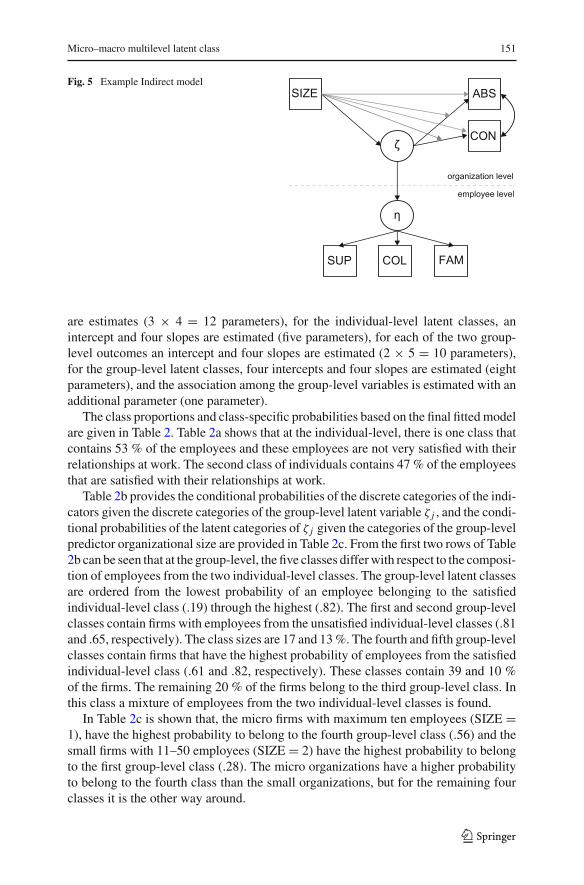
The model can be formally described with seven multinomial logit models: (1)two for the group-level outcomes in which the main effect of ζ j , the main effect oforganizational size and their interaction effect are used as predictors, (2) one for thegroup-level latent variable ζ j inwhich organizational size is used as a predictor, (3) onefor the individual-level latent variable ηi j for which ζ j is a predictor, and (4) three forthe individual-level variables for which ηi j is a predictor. Furthermore, a two-variableassociation among the two firm-level outcomes is added to the model. The model isgraphically displayed in Fig. 5 (the effects that were not significant are colored gray).
The number of classes for the two latent variables are determined following thestepwise procedure of Lukociene et al. (2010) using BIC based on the number ofgroups. This resulted in two classes at the individual-level and five classes at the group-level. The class separation of the latent variables is sufficient to good (Rη
entr = .67and Rζ
entr = .92). Again, Latent GOLD was used to check whether the model isempirically identified.
All effects were significant at the 5% level, except the main effect of organizationalsize and its interaction effect with ζ j on both group-level outcomes. Therefore, theseeffects were removed from the model and the final model contains 36 parameters:for each of the three observed individual-level variables, an intercept and three slopes
123
Micro–macro multilevel latent class 151
Fig. 5 Example Indirect modelABS
ζ
COL
SIZE
FAMSUP
η
employee level
organization level
CON
are estimates (3 × 4 = 12 parameters), for the individual-level latent classes, anintercept and four slopes are estimated (five parameters), for each of the two group-level outcomes an intercept and four slopes are estimated (2 × 5 = 10 parameters),for the group-level latent classes, four intercepts and four slopes are estimated (eightparameters), and the association among the group-level variables is estimated with anadditional parameter (one parameter).
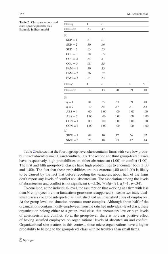
The class proportions and class-specific probabilities based on the final fittedmodelare given in Table 2. Table 2a shows that at the individual-level, there is one class thatcontains 53 % of the employees and these employees are not very satisfied with theirrelationships at work. The second class of individuals contains 47 % of the employeesthat are satisfied with their relationships at work.
Table 2b provides the conditional probabilities of the discrete categories of the indi-cators given the discrete categories of the group-level latent variable ζ j , and the condi-tional probabilities of the latent categories of ζ j given the categories of the group-levelpredictor organizational size are provided in Table 2c. From the first two rows of Table2b can be seen that at the group-level, the five classes differwith respect to the composi-tion of employees from the two individual-level classes. The group-level latent classesare ordered from the lowest probability of an employee belonging to the satisfiedindividual-level class (.19) through the highest (.82). The first and second group-levelclasses contain firms with employees from the unsatisfied individual-level classes (.81and .65, respectively). The class sizes are 17 and 13%. The fourth and fifth group-levelclasses contain firms that have the highest probability of employees from the satisfiedindividual-level class (.61 and .82, respectively). These classes contain 39 and 10 %of the firms. The remaining 20 % of the firms belong to the third group-level class. Inthis class a mixture of employees from the two individual-level classes is found.
In Table 2c is shown that, the micro firms with maximum ten employees (SIZE =1), have the highest probability to belong to the fourth group-level class (.56) and thesmall firms with 11–50 employees (SIZE = 2) have the highest probability to belongto the first group-level class (.28). The micro organizations have a higher probabilityto belong to the fourth class than the small organizations, but for the remaining fourclasses it is the other way around.
123
152 M. Bennink et al.
Table 2 Class proportions andclass-specific probabilitiesExample Indirect model
Class η 1 2
Class size .53 .47
(a)
SUP = 1 .67 .01
SUP = 2 .30 .46
SUP = 3 .03 .53
COL = 1 .58 .05
COL = 2 .34 .41
COL = 3 .08 .55
FAM = 1 .40 .15
FAM = 2 .36 .32
FAM = 3 .24 .53
Class ζ 1 2 3 4 5
Class size .17 .13 .20 .39 .10
(b)
η = 1 .81 .65 .53 .39 .18
η = 2 .19 .35 .47 .61 .82
ABS = 1 .00 1.00 .00 1.00 .00
ABS = 2 1.00 .00 1.00 .00 1.00
CON = 1 .00 .00 1.00 1.00 .00
CON = 2 1.00 1.00 .00 .00 1.00
(c)
SIZE = 1 .09 .10 .17 .56 .07
SIZE = 2 .28 .18 .23 .17 .14
Table 2b shows that the fourth group-level class contains firmswith very low proba-bilities of absenteeism (.00) and conflict (.00). The second and third group-level classeshave, respectively, high probabilities on either absenteeism (1.00) or conflict (1.00).The first and fifth group-level classes have high probabilities to encounter both (1.00and 1.00). The fact that these probabilities are this extreme (.00 and 1.00) is likelyto be caused by the fact that before recoding the variables, about half of the firmsdon’t report any levels of conflict and absenteeism. The association among the levelsof absenteeism and conflict is not significant (r=5.26,Wald=.91, d f =1, p=.34).
To conclude, at the individual-level, the assumption that working at a firm with lessthan50 employees is either fantastic or gruesome is supported, since the two individual-level classes could be interpreted as a satisfied and an unsatisfied class of employees.At the group-level the situation becomes more complex. Although about half of theorganizations containmostly employees from the satisfied individual-level class, theseorganization belong either to a group-level class that encounters low or high levelsof absenteeism and conflict. So at the group-level, there is no clear positive effectof having satisfied employees on organizational levels of absenteeism and conflict.Organizational size matters in this context, since micro organizations have a higherprobability to belong to the group-level class with no troubles than small firms.
123

Micro–macro multilevel latent class 153
6 Discussion
In the current article, two latent class models, referred to as the Direct model andthe Indirect model, are presented that can be used to predict a group-level outcomeby means of multiple individual-level variables by extending an existing method formicro-macro analysis with a single individual-level variable to the multivariate case.Bothmodels involve the construction of a group-level latent class variable based on theindividual-level variables to summarize the individual-level information at the group-level. The group-level latent variable can then be related to other group-level variables,such as a group-level outcome. In the Direct model, the group-level latent classesaffect the individual-level variables directly, while in the Indirect model these areaffected indirectly via an individual-level latent variable. TheDirectmodel seemsmostappropriate when the aim of the research is to construct a typology of groups that affectone or more group-level outcomes. In this situation the within and between componentof the individual-level variables are independent. The Indirect model seems moreappropriate when the individual-level variables are intended to measure an individual-level construct and groups are allowed to differ on the individual-level variable. Thewithin and between component of the individual-level variables are now dependent.Both methods are applied to real data examples.
In the models with a discrete latent variable at each level, the number of classes ofthe latent variables had to be decided simultaneously since the full model was esti-mated at once. Although Lukociene et al. (2010) provided guidelines on how to makethis decision, further research should be devoted to study whether their approach isalso optimal in the current context. Especially when the latent variables are dependent,one might prefer to determine the number of latent classes of the two variables inde-pendently. A stepwise procedure to do this without introducing bias in the group-levelparameter estimates, is presented in Bolck et al. (2004), Vermunt (2010), and Bakket al. (2013). A further limitation of the current method is that the group-level outcomefunctions as an additional indicator of the latent group-level variable. This implies thatthe formation of the group-level classes is affected by the outcome variable. This maybe counter intuitive since the latent variable is intended to predict the outcome. Anadditional advantage of using the stepwise procedure just referred to, is that the latentclasses can not only be defined independent of each other, but also independent of thegroup-level outcome.
Acknowledgments We would like to thank the Survey of Italian Household Budgets for providing datafor the first empirical example. Margot Bennink is supported by a Grant from the Netherlands Organisationfor Scientific Research (NWO 400-09-018).
Open Access This article is distributed under the terms of the Creative Commons Attribution 4.0 Interna-tional License (http://creativecommons.org/licenses/by/4.0/), which permits unrestricted use, distribution,and reproduction in any medium, provided you give appropriate credit to the original author(s) and thesource, provide a link to the Creative Commons license, and indicate if changes were made.
References
Bakk Z, Tekle FB, Vermunt JK (2013) Estimating the association between latent class membership andexternal variables using bias adjusted three-step approaches. Sociol Methodol 43(1):272–311
123

154 M. Bennink et al.
Bank of Italy (2012) Historical database of survey of household income and wealth, 1977–2010Bennink M, Croon MA, Vermunt JK (2013) Micro–macro multilevel analysis for discrete data: a latent
variable approach and an application on personal network data. Sociol Methods Res 42(4):431–457Bolck A, Croon MA, Hagenaars JAP (2004) Estimating latent structure models with categorical variables:
one-step versus three-step estimators. Polit Anal 12(1):3–27CroonMA, vanVeldhovenMJPM(2007) Predicting group-level outcome variables fromvariablesmeasured
at the individual level: a latent variable multilevel model. Psychol Methods 12(1):45–57European Commission (2005) The new SME definition: user guide and model declaration. Publication
Office, BrusselsGoldstein H (2011) Multilevel statistical models, 4th edn. Wiley, ChichesterGoss D (1991) Small business and society. Routledge, LondonGuest DE, Peccei R (2001) Partnership at work: mutuality and the balance of advantage. Brit J Ind Relat
39(2):207–236Lukociene O, Varriale R, Vermunt JK (2010) The simultaneous decision(s) about the number of lower- and
higher-level classes in multilevel latent class analysis. Sociol Methodol 40(1):247–283Preacher KJ, Zyphur MJ, Zhang Z (2010) A general multilevel SEM framework for assessing multilevel
mediation. Psychol Methods 15(3):209–233Skrondal A, Rabe-Hesketh S (2004) Generalized latent variable modeling: multilevel, longitudinal and
structural equation models. Chapman & Hall/CRC Press, Boca RatonSnijders TAB, Bosker RJ (2012) Multilevel analysis: an introduction to basic and advanced multilevel
modeling, 2nd edn. Sage Publications, LondonVan VeldhovenMJPM,Meijman T, Broersen S (2002) Handleiding VBBA: onderzoek naar de beleving van
psychosociale arbeidsbelasting en werkstress met behulp van de vragenlijst beleving en beoordelingvan de arbeid. Stichting Kwaliteitsbevordering Bedrijfsgezondheidszorg, Amsterdam
Varriale R, Vermunt JK (2012) Multilevel mixture factor models. Multivar Behav Res 47(2):247–275Vermunt JK (2003) Multilevel latent class models. Sociol Methodol 33(1):213–239Vermunt JK (2005) Mixed-effects logistic regression models for indirectly observed discrete outcome
variables. Multivar Behav Res 40(3):281–301Vermunt JK (2010) Latent class modeling with covariates: two improved three-step approaches. Polit Anal
18(4):450–469Vermunt JK, Magidson J (2005) Technical Guide for Latent GOLD 4.0: basic and advanced. Statistical
Innovations, Belmont, MAVermunt JK, Magidson J (2013) LG-Syntax User’s Guide: manual for Latent GOLD 5.0 syntax module.
Statistical Innovations, Belmont, MAWilkinson A (1999) Employment relations in SME’s. Empl Relat 21(3):206–217
123