MICROFLUIDIC TECHNIQUES FOR LYSING, PURIFICATION AND

BEAD-BASED DETECTION OF RNA FROM COMPLEX SAMPLES

A DISSERTATION

SUBMITTED TO THE DEPARTMENT

OF MECHANICAL ENGINEERING

AND THE COMMITTEE OF GRADUATE STUDIES

OF STANFORD UNIVERSITY

IN PARTIAL FULFILMENT OF THE REQUIREMENTS

FOR THE DEGREE OF

DOCTOR OF PHILOSOPHY

Anita Rogacs

September 2013

http://creativecommons.org/licenses/by-nc/3.0/us/

This dissertation is online at: http://purl.stanford.edu/wk525zg0251

© 2013 by Anita Rogacs. All Rights Reserved.

Re-distributed by Stanford University under license with the author.

This work is licensed under a Creative Commons Attribution-Noncommercial 3.0 United States License.

ii

I certify that I have read this dissertation and that, in my opinion, it is fully adequatein scope and quality as a dissertation for the degree of Doctor of Philosophy.

Juan Santiago, Primary Adviser

I certify that I have read this dissertation and that, in my opinion, it is fully adequatein scope and quality as a dissertation for the degree of Doctor of Philosophy.

Kenneth Goodson

I certify that I have read this dissertation and that, in my opinion, it is fully adequatein scope and quality as a dissertation for the degree of Doctor of Philosophy.

Thomas Kenny

Approved for the Stanford University Committee on Graduate Studies.

Patricia J. Gumport, Vice Provost for Graduate Education

This signature page was generated electronically upon submission of this dissertation in electronic format. An original signed hard copy of the signature page is on file inUniversity Archives.

iii

IV

V

Abstract This dissertation describes three techniques aimed at automated, sensitive sample

preparation and detection of RNA from complex samples. Microfluidic systems have

advanced the state of the art for a wide number of chemical and biological assays, but

robust and efficient sample preparation remains a major challenge. One of the most

difficult processes is the lysing, purification, and detection of target RNA from whole

blood samples. This dissertation addresses key challenges in each of these RNA

workflow phases.

In the first part of the dissertation, we demonstrate a novel assay for lysing

followed by physicochemical extraction and isotachophoresis-based purification of 16S

ribosomal RNA from whole human blood infected with Pseudomonas Putida. This assay

is unique in that the extraction can be automated on-chip using isotachophoresis in a

simple device with no moving parts, it protects RNA from degradation when isolating

from ribonuclease-rich matrices (like blood), and produces a purified total nucleic acid

(NA) sample which is compatible with enzymatic amplification assays. We show that the

purified RNA are compatible with reverse transcription-quantitative polymerase chain

reaction (RT-qPCR), and demonstrate a clinically relevant sensitivity of 0.03 bacteria per

nanoliter using RT-qPCR.

In the second part of the dissertation, we present a model to aid in design and

optimization of a wide range of electrophoresis (including isotachophoresis) assays. Our

model captures the important contributors to the effects of temperature on the observable

electrophoretic mobilities of small ions, and on solution ionic strength, conductivity and

VI

pH; the most relevant parameters in molecular reactions and separation assays. Our

temperature model includes relations for temperature-dependent viscosity, ionic strength

corrections, degree of ionization (pK), and ion solvation effects on mobility. We

incorporate thermophysical data for water viscosity; temperature-dependence of the

Onsager-Fuoss model for finite ionic strength effects on mobility; temperature-

dependence of the extended Debye-Huckel theory for correction of ionic activity; the

Clarke-Glew approach and tabulated thermodynamic quantities of ionization reaction for

acid dissociation constants as a function of temperature; and species-specific, empirically

evaluated correction terms for temperature-dependence of Stokes’ radii. We incorporated

our model into a MATLAB-based simulation tool we named Simulation of Temperature

Effects on ElectroPhoresis (STEEP). We validated our model using conductance and pH

measurements across a temperature variation of 25°C to 70°C for a set of electrolytes

routinely used in electrophoresis. The model accurately captures electrolyte solution pH

and conductivity, including important effects not captured by simple Walden type

relations.

In the third and final part of the dissertation, we introduce a cost-effective and

simple-to-implement method for direct detection of RNA, by analyzing images of

randomly distributed multicolor fluorescent beads bound by the target molecule. We term

our method particle imaging, tracking and collocation (PITC). We use a fairly standard

epifluorescence microscopy setup fitted with an off-the-shelf dual view color separator

attachment which images fluorescence emission at two wavelengths onto two respective

halves of a single CCD image array. We perform automated analysis of these two color

channels to track thousands of particle images in either or both wavelengths, and we track

VII

particle image motion in time and space. We can quantify particle image wavelength (or

wavelength ratio), absolute intensities, and particle image diameter. We also perform

cross-correlation image analyses on this multi-wavelength data to track particle

collocations and the degree of correlation of particle motion. Particles or cells can be

suspended in solution and flowed through a wide variety of microchannels (with optical

access for image collection). Particles can be transported through the detection region via

electrophoresis and/or pressure driven flow, to increase throughput of analysis. We here

introduce and evaluate the performance of our method. We use Monte Carlo simulations

to demonstrate robustness of the algorithm and optimize algorithm parameters. We

present an experimental demonstration of the method on challenging image data,

including flow of randomly distributed Brownian particles and particle populations which

undergo particle-to-particle binding. We show results of bead collocation measurements

on bead-to-bead binding created by the E.coli 16S rRNA gene.

VIII

Acknowledgments I was only 18 when I first walked the grounds of The Farm, dreaming of a life at

this prestigious University. It was only a month after I moved here from Hungary, leaving

my family and friends behind. I sat on the fields of the Oval on Palm Drive, thinking how

ridiculous this dream was, and that I should consider myself lucky to even talk to

someone attending here. Many years have passed since that day, and I find myself

wondering, how I got here. Frankly, it does not take much effort to find the answer to this

question: I had a dream and I surrounded myself with the people I admired the most.

Dreaming for a better, successful and rewarding life is easy. That was my part. But the

rest of this story is about the amazing people I met during this journey. I am humbled by

the number of individuals who have blessed me with their time, their patience, and their

knowledge.

First, I would like to thank my research advisor, Professor Juan Santiago, for

supervising my doctoral research and for guiding me through the natural ups and downs

of scientific research. Juan is a brilliant researcher with an infectious passion for science

and teaching. He motives by example, sets high expectations (definitely higher than what

you think you can achieve), and gives sometimes harsh, but always honest feedback on

progress and results. (I have heard others refer to this as “extreme professional honesty.”)

I find his professional honesty one of the most refreshing and effective aspects in his

advising methods. The greatness in his approach lies in his transparent motivation: Above

all he wants you to succeed. He takes his role as your mentor and adviser personally.

While his passion is science, his mission is preparing you for a life in research. Thanks to

his great efforts and care, I have grown infinitely more capable and confident in my

IX

work, to a point where I dare to dream bigger and better. I am incredibly fortunate to call

him my mentor and adviser.

I am also very grateful for Professor Kenneth Goodson, who was my research

adviser during the first three years of graduate school. The first year at Stanford can be

scary, overwhelming and hectic. My meetings with Ken were always constructive and

productive, as he rose above the noise of my frantic concerns and advised me to prioritize

and focus my attention on the issues with greatest impact and importance. He is a man of

few, but carefully selected words. I always admired his professional and personal wisdom

and calm demeanor. He has given me much invaluable personal and professional career

advice for which I have benefited greatly. I would also like to thank Professor Thomas

Kenny for his advice, guidance and support on my dissertation and for his genuine

curiously and interest in my work and career plans. I regard the opportunities I had for

interaction with Prof. Kenny as an absolute privilege.

I want to thank my undergraduate research adviser, Prof. Jinny Rhee, who has

taken me under her wings, introduced me to the word of research, helped me write my

first conference paper and continued to cheer me on during this journey. Jinny, you have

been a wonderful mentor and a great friend. I am also incredibly thankful for the support

and guidance I received from the team at HP Labs: Chandrakant Patel, Amip Shah, and

Cullen Bash. I especially thank Amip for the many lunch meetings, thought-provoking

discussions, and his unwavering support and mentorship.

I thank all my lab mates in both the Santiago and the Goodson labs. I greatly

appreciate the immense knowledge (professional and personal) I gained from interacting

with Jeremy, Shilpi, Lewis, Julie, Joe, Milnes, Amy, Moran, Supreet, Giancarlo, and

X

Yatian. I thank you and the rest of the group(s) for everything you taught me, for your

willingness to share ideas, and for always being supportive and encouraging. I especially

thank Lewis Marshall and Julie Steinbrenner, who spent many hours building

experiments, taking data, and debating problems and solutions with me. But what I

cherished the most was the time we spent together burning off stress by either running or

rock climbing. You guys rock (pun intended)! I admire you both for your wits, humor

and positive attitude. I am lucky to have found such great friends in lab.

I also want to give special thanks to our administrators, Cecilia Gichane-Belle and

Linda Huber, for their unwavering support. Without you, we simply could not function.

I gratefully acknowledge the financial support I received from the National

Science Foundation and from the Sandia National Laboratories Campus Executive

Graduate Research Project. Receiving these fellowships allowed me to pursue interests

that otherwise would not have been possible.

Finally, I want to say that I could not have done any of this without my family. I

am eternally grateful to my parents who have instilled in me the great value of hard work,

and the deep sense of accomplishment it offers. I am also very grateful for my family

here, Jeremy, Jane and John, for supporting me at every step of this long journey. I am

blessed to have a loving husband who understands me, who makes me laugh, and who

inspires me to be a better person every day. Jeremy has seen me at my best and at my

worst and has kept me anchored in reality throughout. I am so thankful to have him in my

life. Lastly, I want to give huge thanks to my closest friends who reminded every day that

life outside the lab is fun, exciting and beautiful. Jeremy, Zoli, Ildiko, Yasmin, Shilpi,

and Ashley: thanks for keeping me balanced all these years. You are the family I chose.

XI

Table of Contents

ABSTRACT………………………………………………………………………………...II

ACKNOWLEDGMENTS…………………………………………………………………....IV

TABLE OF CONTENTS……………………………………………………………………..V

LIST OF TABLES…………………………………………………………………………VII

LIST OF FIGURES……………………………………………………………………….VIII

1 INTRODUCTION ............................................................................................................. 1

1.1 Why target Ribonucleic acid (RNA) ............................................................................... 1

1.2 Workflow of RNA analysis .............................................................................................. 2

1.3 Sample preparation .......................................................................................................... 6

1.3.1 Sample Matrix Interference ........................................................................................ 6

1.3.2 Traditional purification methods ............................................................................... 6

1.4 Temperature effects on RNA reactions and separations ............................................ 10

1.4.1 Enzyme-based reactions, hybridization stringency and reaction rates .................... 10

1.4.2 Electrophoretic separation ....................................................................................... 12

1.5 Sequence-specific RNA detection .................................................................................. 14

1.6 Scope of thesis ................................................................................................................. 17

2 BACTERIAL RNA EXTRACTION AND PURIFICATION FROM WHOLE HUMAN BLOOD

USING ISOTACHOPHORESIS .............................................................................................. 19

2.1 Introduction .................................................................................................................... 19

2.2 Materials and methods................................................................................................... 23

2.3 Results and discussion .................................................................................................... 29

2.3.1 Assay design and evaluations ................................................................................... 29

XII

2.3.2 Demonstration of extraction purity and compatibility with RT-qPCR ..................... 33

3 TEMPERATURE EFFECTS ON ELECTROPHORESIS ..................................................... 38

3.1 Introduction .................................................................................................................... 38

3.2 Theory ............................................................................................................................. 42

3.2.1 Walden’s rule ........................................................................................................... 42

3.2.2 Ion solvation effect on limiting ion mobility ............................................................. 44

3.2.3 Ionic strength correction of limiting mobility: actual ion mobility .......................... 46

3.2.4 Degree of ionization: effective mobility ................................................................... 49

3.2.5 Solution method for temperature model ................................................................... 55

3.2.6 Quantifying the aggregate effect of temperature dependences unrelated to viscosity

56

3.2.7 Stand-alone simulation tool for temperature-dependent electrolyte properties ...... 57

3.3 Materials and Methods .................................................................................................. 60

3.4 Results and discussion .................................................................................................... 61

3.4.1 Predictions of effective mobility, conductivity, and pH ............................................ 61

3.4.2 Additional electrolyte examples ............................................................................... 67

3.4.3 Temperature model validation ................................................................................. 70

4 PARTICLE TRACKING AND MULTISPECTRAL COLLOCATION METHOD FOR

CYTOMETRY-LIKE AND PARTICLE-TO-PARTICLE BINDING ASSAYS ............................. 76

4.1 Introduction .................................................................................................................... 76

4.2 Materials and methods ................................................................................................... 80

4.2.1 Overview of Collocation method .............................................................................. 80

4.2.2 Reagents and materials ............................................................................................ 81

4.2.3 Imaging and particle residence time requirements .................................................. 83

4.2.4 Particle tracking and collocation algorithm ............................................................ 85

4.3 Validation and Performance ......................................................................................... 95

4.3.1 Monte Carlo simulations .......................................................................................... 95

4.3.2 Image SNR and median collocation threshold ......................................................... 96

XIII

4.3.3 Particle density and monitoring time ..................................................................... 100

4.4 Experimental demonstration of cytometry-like data and collocation analysis ....... 103

4.4.1 Time resolved collocation coefficient ..................................................................... 104

4.4.2 Cytometry-like fluorescence data ........................................................................... 105

5 CONCLUSIONS, CONTRIBUTIONS, AND RECOMMENDATIONS ................................... 108

5.1 Summary of conclusions .............................................................................................. 108

5.1.1 Bacterial RNA Extraction and Purification from Whole Human Blood Using

Isotachophoresis ................................................................................................................. 108

5.1.2 Temperature Effects on Electrophoresis ................................................................ 109

5.1.3 Particle Tracking and Multispectral Collocation Method for Cytometry-Like and

Particle-to-Particle Binding Assays .................................................................................... 110

5.2 Summary of major contributions ............................................................................... 111

5.2.1 Bacterial RNA Extraction and Purification from Whole Human Blood Using

Isotachophoresis ................................................................................................................. 111

5.2.2 Temperature Effects on Electrophoresis ................................................................ 112

5.2.3 Particle Tracking and Multispectral Collocation Method for Cytometry-Like and

Particle-to-Particle Binding Assays .................................................................................... 113

5.3 Recommendations for future work ............................................................................. 114

5.3.1 Bacterial RNA Extraction and Purification from Whole Human Blood Using

Isotachophoresis ................................................................................................................. 114

5.3.2 Temperature Effects on Electrophoresis ................................................................ 114

5.3.3 Particle Tracking and Multispectral Collocation Method for Cytometry-Like and

Particle-to-Particle Binding Assays .................................................................................... 115

6 BIBLIOGRAPHY ......................................................................................................... 117

7 APPENDIX A. ITP COMPATIBLE LYSIS METHODS .................................................... 143

8 APPENDIX B. PARTICLE HYBRID ANALYSIS ............................................................. 152

XIV

List of Tables Table 3.1 Examples of temperature models of aqueous electrolyte solutions from the last

25 years. Effects captured by each model are categorized into two types: pK or

actual mobility, μo corrections. Abbreviation ‘dpK/dT’ indicates that only tabulated

values of this slope were presented. ‘pKC-VC’ and ‘pKC-CG’ represent models

which account for temperature dependence of pK using van’t Hoff or the higher

accuracy Clark-Glew model, respectively. Viscosity corrections using of the Walden

rule type are indicated with ‘W’. We also list models which account for the

temperature dependence of ionic strength corrections of activity coefficient (‘ISC-

pK’) and actual mobility (‘ISC-μ’). .......................................................................... 40

Table 3.2. List of chemical species mobility, μ, (in 109 m2V-1s-1) , pK, standard free

enthalpy of ionization,∆Ho, (in J mol-1) standard free specific heat of

ionization,∆Cpo , (in J K-1 mol-1) values defined at 25°C, as used in main paper. .... 59

Table 3.3 Summary of full model (labeled “Current” in Figures 1-3) and limiting models

used for comparing the various sources of temperature effects on effective ionic

mobility. The values )(, θµ zi and )(, Tziµ are evaluated using Eq (3.22). )(, θzig ,

and )(, Tg zi are evaluated using Eq (3.20). The assumptions made for the limiting

models include temperature insensitivity of ion solvation, )1( =iβ , temperature-

independent degree of ionization ( 0/ =dTdpK ), and temperature independent ionic

strength corrections ))"(.(" TfcorrIS ≠ . T is the operating temperature and θ is the

reference temperature (25°C). ................................................................................... 62

XV

Table 3.4 Experimental validation of the temperature model for electrolyte solution pH at

25°C and 70°C. Uncertainty values indicate 95% confidence on the mean. ............ 73

Table 3.5 Summary of predictions and measurements of pH and conductivity for six

additional electrolyte solutions at temperatures 25°C and 70°C. ............................. 74

Table 4.1. Brief review and comparison of multispectral particle analysis and

enumeration techniques. We compare the capabilities and features of the current

technique (PITC) with FCM and LSC. .................................................................... 79

XVI

List of Figures Figure 1.1 (Top) Traditional RNA workflow and example techniques. The workflow

typically involves four phases: extraction, separation (involving purification and

quantitation), reaction and detection. We here show representative example methods

for each of the phases. (Bottom) Schematic of thesis contributions in the

corresponding RNA workflow phases are listed in grey blocks. The details of these

contributions are described in Chapter 2, 3 and 4, respectively. ................................ 4

Figure 2.1 Schematic of the ITP-based NA purification from a complex biological

sample such as blood lysate. After dispensing the lysate containing TE into the well

(top left of schematic and top channel), an electric field was applied (middle

channel), and the total NA migrated into the microchannel, where it was focused and

purified into the ITP interface. This process enables PCR inhibitors (including

proteins) to remain unfocused in the TE well (e.g., cations) or in channel regions

well separated from the ITP zone. After the total NA elutes into the LE well (bottom

channel), the content was extracted using a standard pipette. We then split this

extract into two equal 4 ul aliquots for parallel off-chip RT-qPCR and qPCR

analyses. .................................................................................................................... 22

Figure 2.2 Schematic summarizing protocol with one mixing and two dispensing steps

for otherwise automated on-chip RNA extraction from whole blood. TE mixed with

lysate (brown) contains target nucleic acid (green), proteins, and potential PCR-

inhibiting chemistries. Appropriate selection of trailing and leading ions enables

selective focusing of target nucleic acid while leaving PCR inhibitors behind. The

XVII

detail view shows on-chip extraction of RNA from blood stained with SYBR Green

II, focused into a concentrated zone. The amplification plot shows the result of

alkaline based lysing (enhanced with Triton X-100, DTT and carrier RNA) of total

nucleic acid from whole blood spiked with P. Putida at 30 ¢/nL, followed by

purification of total NA from lysate using ITP. The NA collected from the output

well was split to perform both RT-qPCR and qPCR to verify successful extraction of

16S rRNA (red dotted) and 16S rDNA (red bold dashed). For the negative control

template (uninfected blood) RT-qPCR amplified 16S rRNA (blue solid line) above

30 cycles and qPCR did not amplify 16S rDNA within 40 cycles, as expected. ...... 25

Figure 2.3 Microfluidic chip geometry. We performed isotachophoretic purification of

NA on a L1-4 = 60.7 mm long, 120 um wide, 35 um deep Crown glass microchannel

(NS12A) interfaced with 3.5 mm deep and 3.5 diameter wells from Caliper Science

Life Sciences, CA. The wells sit open and exposed to room air during ITP. ........... 27

Figure 2.4 Main plot shows a representative trace of measured current versus time.

Current can be used to control the timing of the experiment. Inset: Overlayed raw

current measurements for 18 experiments (13 infected samples shown in figure 2 of

the manuscript, and 5 negative controls) performed on a single chip. These repeats

have a coefficient of variation of less than 6%. ........................................................ 28

Figure 2.5 Experimental demonstrations of the combined effect of reducing agent (DTT)

and carrier RNA on ITP-based RNA purification from bacteria infected human

blood. The bars show RT-qPCR threshold cycles for 16S rRNA extracted from

blood spiked with P. putida cells. All negative controls for RT-qPCR (RNA

XVIII

extracted from uninfected blood) amplified above 30 cycles. We show results from

four sets of experiments. Lysing in the presence of DTT and carrier RNA yields

consistent and low threshold amplification cycles for two different bacterial cell

densities. In their absence, all bacterial RNA extractions failed, or were significantly

compromised. We believe that the observed effect is primarily due to the presence of

DTT. However, we hypothesize that carrier RNA would have significant effect on

extraction efficiency at very low RNA concentration (which includes RNA from the

background matrix). The latter hypothesis is supported by the typically higher

variation in threshold target levels for the “no DTT, no carrier RNA” case at lower

bacteria concentrations, such as the example data shown here. NA indicates no

amplification within 40 cycles. ................................................................................. 32

Figure 2.6 Example on-chip fluorescence images and experimental integrated

fluorescence curves of extracted nucleic acid ITP zones stained with SYBR Green

II. The inset fluorescence profile and image on the top right shows RNA extracted

from uninfected blood (negative control). The main fluorescence plot and image at

the bottom corresponds to a typical run with blood infected with P. putida at 30 ¢/nL

concentration. We corrected the ITP-focused nucleic acid fluorescence images by

subtracting a background fluorescence image and dividing this by the difference

between a flat field image and the background image (see the supplementary

information document of Persat et al. for further details). For the fluorescence peak

distribution, we integrated image intensities along the width of the channel and show

here versus distance along the channel’s main axis. These image analysis and

XIX

fluorescence integrations were performed using MATLAB (The Mathworks, MA).

................................................................................................................................... 34

Figure 2.7 RT-qPCR threshold cycles for 16S rRNA extracted from whole human blood

infected with P. putida using our DTT- and carrier-RNA-assisted, alkaline-based

lysing and ITP purification protocol. Plot contains results for a total of 13

experiments, four at 0.03 ¢/nL and three each at 0.3, 3 and 30 ¢/nL bacterial cell

concentrations. All negative controls for RT-qPCR (RNA extracted from uninfected

blood) amplified above 30 cycles, as expected (not shown). Threshold amplification

cycles for the (non RT) qPCR reactions targeting DNA were above 30 for all

experiments, also demonstrating our sensitivity to RNA versus DNA. ................... 35

Figure 2.8 Shown are the raw reverse transcription polymerase chain reaction (RT-

qPCR) amplification curves for the data shown in Figure 2 of the main paper for P.

putida 16S rRNA. P. putida was spiked into whole human blood to final

concentration of 0.03, 0.3, 3, and 30 ¢/nL. We performed RT-qPCR using Power

SYBR Green RNA-to-CT 1-Step Kit from Applied Biosystems with 150 nM forward

(5'-CAAAACTGGCAAGCTAGAGTACG) and 150 nM reverse

(5'-TAAAATCTCAAGGATTCCAACGGCT) primers, with the following thermal

profile: 30 min initial hold at 48°C, followed by 10 min hold at 95°C and 40 cycles

composed of 15 s denaturation at 95°C and 1 min annealing and extension at 60°C.

Negative RT-qPCR reactions (template: uninfected blood), and all PCR reactions

amplified above 30 cycles. ........................................................................................ 36

XX

Figure 3.1. Predicted electrophoretic mobility of Cl- in solution containing 200 mM Tris

and 100 mM HCl as a function of temperature. The pH of this simple buffer tracks

closely temperature dependent value of pK as expected. However, the degree of

Tris ionization is determined by the chloride ion whose molar density is insensitive

to pH. Therefore, this electrolyte system maintains constant ionic strength with

temperature. The simple ‘SSC’ model is fairly accurate here which suggest that the

source of the non-viscosity related temperature dependence is due to the change in

the hydration shell of the chloride ion. ..................................................................... 64

Figure 3.2. Predicted electrophoretic mobility versus temperature of boric acid anion

(borate) in solution containing 20 mM ethanolamine and 20 mM boric acid. Increase

in temperature results in strong drop in pK of ethanolamine and a moderate drop in

the pK of boric acid, resulting in an overall decrease in pH (top inset). Here, the

most prominent contribution to both anion mobility and ionic strength, I (bottom

inset) is due to the sharp decrease in degree of ionization of boric acid (hence the

proximity of ‘pKC’ model to ‘Current’). The large, positive value of log10f (bottom

inset) shows how this effect opposes contributions from the decreasing viscosity to

conductivity. Ultimately, these opposing effects are also reflected by the shallow

mobility curve (main plot). Predictions based on Walden’s rule here overestimate

the anion mobility by 116% (and buffer conductivity by 106%). ............................ 65

Figure 3.3 Predicted electrophoretic mobility of a trivalent ion, citrate, in a solution

containing 200 mM Bis-tris and 50 mM citric acid. For simplicity we show only the

pK of the trivalent anion of citric acid (citrate ion, z = -3). Increase in temperature

results in a strong drop in pK of Bis-tris and a mild increase in the pK of citrate ion,

XXI

resulting in an overall reduction in pH (top inset). The sharp decrease in the degree

of ionization of the citrate ion contributes strongly to the decrease in ionic strength

(bottom inset), which would suggest a considerable effect on its effective mobility

(see limiting model ‘pKC’). However, the ion’s multivalent nature makes citrate

extremely sensitivity to changes in the ionic strength. Therefore, the temperature-

induced reduction in ionic strength is accompanied by a reduction in the magnitude

of the Onsager-Fuoss correction term. The two effects offset each other and so the

net effects are well approximated by the Walden model (which nearly exactly

overlies the Current model). ..................................................................................... 66

Figure 3.4 Prediction of anionic (citrate) and cationic (potassium) mobilites in an

electrolyte solution composed of 50 mM potassium citrate (pK-3 = 6.396, pK-2 =

4.761, pK-1 = 3.128) mixed with 200 mM Bis-tris (pK = 6.484) (Solution 2, in Table

3 of paper). Left plot shows the predicted electrophoretic mobility of a trivalent ion,

citrate. In the inset, we show only the pK of the trivalent and divalent anion of citric

acid, which lie far from the solution pH, indicating no change in degree of

ionization. Thus we can attribute the change in the effective mobility of citrate to

temperature variation of ionic strength correction terms. Right plot shows the

predicted electrophoretic mobility of a monovalent cation, potassium. The simple

‘SSC’ model is fairly accurate here which suggest that the dominant source of the

non-viscosity related temperature dependence is due to the change in the hydration

shell of the potassium ion. The residual deviation of ‘SSC’ from the ‘Current’

solution is due to the temperature dependence of ionic strength correction, captured

XXII

by ‘ISC’. Limiting models ‘SSC’ and ‘pKC’ (and ‘pKC’ on the left plot) are not

plotted as they nearly perfectly overlap the W curve. .............................................. 68

Figure 3.5 Predicted electrophoretic mobility versus temperature for HEPES (anion) in

the solution of 30 mM Tris and 30 mM HEPES (Solution 3, in Table 3 of main

paper). Increase in temperature results in a strong drop in the pK of Tris and a

moderate drop in the pK of HEPES, resulting in an overall decrease in pH (inset).

Here, the most prominent contribution to anion mobility is due to the sharp

reduction in degree of ionization of HEPES (hence the proximity of ‘pKC’ model to

‘Current’). Predictions based on Walden rule here overestimate the anion mobility

by 30% at 70°C. Limiting models ‘SSC’ and ‘ISC’ are not plotted as they nearly

perfectly overlap the W curve. .................................................................................. 69

Figure 3.6 Predicted electrophoretic mobility versus temperature of acetate (anion) in a

solution containing 30 mM Tris and 15 mM acetic acid (Solution 4, in Table 3.3).

Here, ionic strength of solution containing cation (Tris) and titrant (acetic acid) are

determined by the molarity of the fully-ionized acetic acid. While the pH varies with

temperature dictated by the pK(T) function of the Tris, the large difference (>2 units

for all T) between acetate pK and solution pH ensures that acetic acid remains fully

ionized. Therefore, the acetate mobility predictions based on Walden’s rule estimate

anion mobility fairly accurately, within ~4%. Limiting models ‘SSC’, ‘ISC’, and

‘pKC’ are not plotted as they nearly perfectly overlap the W curve. ....................... 70

Figure 3.7 Experimental validation of the temperature model. Shown are theory curves

along with respective conductivity (σ) measurements (raw data). The measurements

XXIII

are three realizations per condition (symbols clustered at each temperature) for the

following electrolyte solutions: 20mM ethanolamine & 20mM boric acid (∆); 200

mM Bis-tris & 50 mM citric acid (X); 30 mM Tris & 15 mM HEPES (□); and

30mM Tris & 15 mM acetic acid (○). The factor f is defined as σ(θ)η(θ)/σ(T)η(T),

where θ = 25℃, and η is dynamic viscosity. For the ethanolamine buffer, Walden’s

rule prediction for σ at 70°C would result in 75% error. .......................................... 71

Figure 4.1. Particle imaging, tracking and collocation for particle monitoring and

particle-to-particle binding assays. A two-color version is shown here, but the

system is easily scalable to four colors using off-the-shelf instrumentation. A typical

experiment involves (1) loading a solution containing particles emitting in the red

and green into a microchannel; (2) electrophoresing the particles through a detection

region with optical access; and (3) imaging at a user-specified rate using a

microscope equipped with dual-view system and high-sensitivity CCD camera. The

dual-view system chromatically separates the particle images into separate spatial

domains on the CCD array. The PITC algorithm determines location and in-plane

velocity vectors of each particle in one spectral channel. This analysis is used to

track the coordinates, image size, and fluorescence intensity of the individual

particles in time. The subregions surrounding the particles in channel 1 are identified

and tracked then cross-correlated with the corresponding subregions in the other

channel. The persistence (in time) of a high cross-correlation signal indicates

deterministically bound particles. ............................................................................. 80

Figure 4.2. Fluidic channel architecture and loading protocol used in demonstration of

particle imaging, tracking and collocation method. A poly(methyl methacrylate),

XXIV

PMMA, microfluidic fluidic chip with dimensions (10 cm x 2 mm x 150 µm) is

loaded with the buffered bead suspension. The output well was filled with 50 µl of 1

M Tris-HCl (pH 8) buffer. The loading well was filled with the same buffer

containing 25% Pluronic F-127 solution in order to reduce pressure driven flow.

Platinum electrodes were placed in the loading and output well and electrophoresis

was initiated by applying 100 µA across the microchannel. In a typical experiment,

we record 200 chromatically separated particle images at a frequency of 1Hz.

During this time, order 1,000-10,000 unique beads traverse through the field of

view. .......................................................................................................................... 83

Figure 4.3. PITC algorithm structure. Each image sequence contains data for thousands

of unique particles. After registration of the two images, the algorithm proceeds in

two main phases. The first phase quantifies local drift particle velocities using

micron resolution particle image velocimetry (micro-PIV). Unique particle images

in Channel 1 (Ch1) are then identified, located and characterized via the particle

mask correlation and particle characterization (PMC-PC) method. The particle

image intensity and radius are evaluated using a non-linear Gaussian fitting routine.

The algorithm then combines results of PMC-PC and micro-PIV for a particle

tracking velocimetry (PTV) subroutine enhanced by Kalman filter and χ2-testing

method (KC-PTV). This analysis results in accurate determination and tracking of

the location of each particle over time and space. The second phase of the algorithm

cross-correlates subregions surrounding the particle locations identified in Ch1 with

corresponding subregions in the registered Ch2. Ch2 particle characteristics, such as

radius and total fluorescence, are evaluated using the Gaussian fitting subroutine.

XXV

Thresholds for intensity, size, velocity, and correlation coefficient are applied at

each step to eliminate spurious results. ..................................................................... 86

Figure 4.4. Example of misaligned (initial) and aligned (final) bright-field images of two

spectral channels recorded with a quad-view imager (Micro-Imager, Photometrics,

Tucson, AZ), used here in dual-view mode. The images are plotted using Matlab’s

function, imshowpair, which displays the differences between two images. We used

alpha blending to overlay the two spectral channel images before (left) and after

(right) image registration. Note, alpha blending is the process of combining a

translucent foreground color with a background color, which produces a new

blended color. These test images were taken with a 20x objective with a numerical

aperture of 0.5. .......................................................................................................... 87

Figure 4.5. Histogram of the number of particles that were tracked for 1 to 20 frames.

Left: Simulated particle density was set to 100 particles/domain (LIP /Lch = 5.1). The

PMC method relies on brightness patterns for identification of particles. When SNR

is too low (SNR ≤ 6), the brightness patterns are distorted and particles are not easily

identified. Right: SNR for Monte Carlo simulated images were set to 100. PMC

method fails if particle brightness pattern is overly affected by neighboring particles

and Kalman filter and χ2 test will fail as trajectories of closely spaced particles

become indistinguishable. As the inter-particle distance decreases, the particles can

be tracked successfully for progressively shorter times as they are lost due to particle

crowding. For LIP /Lch ≤ 3.6 large fractions of these particles are tracked for shorter

times than that required for collocation (i.e., the minimum evolution time, tch,

defined in Eq. 4.2). .................................................................................................... 97

XXVI

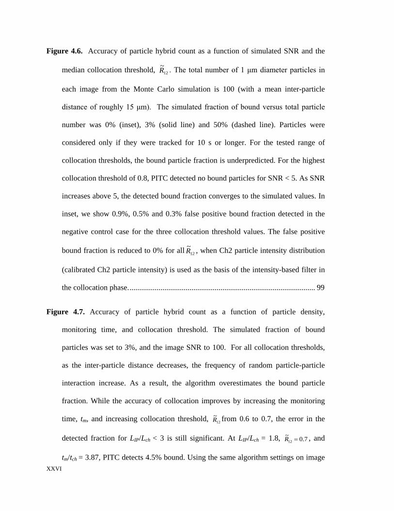
Figure 4.6. Accuracy of particle hybrid count as a function of simulated SNR and the

median collocation threshold, 12~R . The total number of 1 μm diameter particles in

each image from the Monte Carlo simulation is 100 (with a mean inter-particle

distance of roughly 15 μm). The simulated fraction of bound versus total particle

number was 0% (inset), 3% (solid line) and 50% (dashed line). Particles were

considered only if they were tracked for 10 s or longer. For the tested range of

collocation thresholds, the bound particle fraction is underpredicted. For the highest

collocation threshold of 0.8, PITC detected no bound particles for SNR < 5. As SNR

increases above 5, the detected bound fraction converges to the simulated values. In

inset, we show 0.9%, 0.5% and 0.3% false positive bound fraction detected in the

negative control case for the three collocation threshold values. The false positive

bound fraction is reduced to 0% for all 12~R , when Ch2 particle intensity distribution

(calibrated Ch2 particle intensity) is used as the basis of the intensity-based filter in

the collocation phase. ................................................................................................ 99

Figure 4.7. Accuracy of particle hybrid count as a function of particle density,

monitoring time, and collocation threshold. The simulated fraction of bound

particles was set to 3%, and the image SNR to 100. For all collocation thresholds,

as the inter-particle distance decreases, the frequency of random particle-particle

interaction increase. As a result, the algorithm overestimates the bound particle

fraction. While the accuracy of collocation improves by increasing the monitoring

time, tm, and increasing collocation threshold, 12~R from 0.6 to 0.7, the error in the

detected fraction for LIP/Lch < 3 is still significant. At LIP/Lch = 1.8, 7.0~12 =R , and

tm/tch = 3.87, PITC detects 4.5% bound. Using the same algorithm settings on image

XXVII

sets with lower particle density, PITC detects 3.23%, 2.87 % and 3.06% bound

particle fractions at LIP/Lch of 3.6, 5.1 and 7.2, respectively. .................................. 102

Figure 4.8. Collocation particle imaging for DNA detection. A solution containing red

and green beads was mixed with target DNA in a hybridization buffer. Bead doublet

formed when Probe 1 on red fluorescence bead (Bead 1) and Probe 2 on green

fluorescence bead (Bead 2) are hybridized to the target DNA sequence. The bead-

DNA mixture was electrophoresed in a channel with a transparent top wall and

visualized using a microscope equipped with a dual-view system and high-

sensitivity CCD camera. ......................................................................................... 103

Figure 4.9. Measured normalized cross-covariance coefficients between Ch1 and Ch2

particle images of a bead suspension containing two sets of oligo-conjugated

polystyrene beads (one red and one green) in the presence of complimentary DNA.

The plot shows 50 representative traces (20 of them were judged as bound by the

algorithm). The PDF of the covariance coefficients are plotted on the right hand side

of the trace plot. The collocation traces of the bound red beads (solid black) remain

relatively high during the 8 s of monitoring time, indicating deterministic interaction

between Ch1 and Ch2 beads. .................................................................................. 105

Figure 4.10. Multicolor bead hybrid fluorescence in a DNA-induced bead-to-bead

binding assay. Algorithm parameters were set to 2/ ≅chm tt and coIDR ,~

= 0.65. Here

we show overlaid results of two particle tracking approaches. In first approach, red

beads were tracked and cross-correlated with green channel. In the second approach,

green beads were tracked and cross-correlated with red channel. The green and red

XXVIII

markers correspond to green and red fluorescent bead singlets. The purple

subpopulations on the scatter plot represent the green beads that were judged by the

algorithm as collocated with the red beads (G-R). The blue subpopulation was

obtained with the second approach (R-G). When DNA is present in the bead

suspension, 33% of red and 41% of green beads were judged as bound. In the

absence of DNA, 0.8% of red and 1.6% of green beads were judged as

deterministically bound. .......................................................................................... 107

1

1 Introduction

1.1 Why target Ribonucleic acid (RNA)

RNA transcripts within a cell can be broadly classified as ribosomal RNA

(rRNA), transfer RNA (tRNA), messenger RNA (mRNA), and small RNAs.1 rRNA is the

most abundant RNA component in the cell. The abundance of rRNA allows it to be

exploited as a control signal for total RNA mass, as a set of molecular weight markers for

electrophoresis, and as a biomarker for detection of bacterial infection.2, 3 Transfer RNA

is responsible for transporting amino acids to the ribosome to support protein synthesis

and is a target of genetic and metabolic research.4 Messenger RNA is the most diverse of

all RNA transcripts and it is the central driver of cell phenotype. The abundance levels of

an individual mRNA sequence might range from a single copy to thousands of copies per

cell.5 The expression levels of low to moderate abundance mRNA can provide

information on the clinical status and outcome of cancer6 and/or the effectiveness of

applied treatment.7 Housekeeping genes typically make up the set of high abundance

mRNAs and are often used to normalize gene expression levels of other relevant

mRNAs.8 Finally, micro-RNAs (miRNAs) are subset of transcripts, which only recently

gained significant attention. They serve essential and diverse physiological functions

such as differentiation and development, proliferation, and maintaining cell type

phenotypes; and will likely serve as the basis for novel therapies and diagnostic tools in

the future.9 The menagerie of RNA species and their functions is still expanding, and it is

becoming clear that RNA species can play roles in post-transcription RNA modification,

DNA modification, telomerase extension, and a range of other functions.

2

1.2 Workflow of RNA analysis

Figure 1.1 illustrates a typical process flow for RNA analysis, which includes

steps such as RNA extraction, purification, quantitation, reaction and detection. The

choice for the method of RNA extraction or lysis is primary governed by the

subpolulation of RNA (e.g.: tRNA, mRNA, rRNA) that is of interest, the biological

source of RNA (e.g.: bacteria, virus, fungi, host mammalian cell), and of the sample

matrix (e.g.: urine, saliva and blood). Due to the enormous complexity of the extraction

process, such protocols are often empirically derived and optimized. Many efficient

methodologies which accommodate the expedient isolation of RNA have already been

developed1 and can be categorized into chemical, thermal, mechanical and electrical

based methods. After extraction, the RNA is ideally purified from interfering compounds.

The most common methods include liquid phase and solid phase extractions (See Section

1.3.2 for detailed discussion). The purified RNA quantity and quality is subsequently

analyzed via electrophoretic separations (for example, the Bioanalyzer10, 11). While the

presence of unique RNA sequence can be directly detected with various transduction

methods, its instable nature,12-14 or requirement for sequence amplification, often

necessitates its conversion to its complimentary DNA (cDNA) sequence via reverse-

transcription (RT). The conversion of RNA to DNA is accomplished by an enzyme,

called reverse transcriptase, and the process takes approximately 45 min at elevated

temperature. This process is then followed by either polymerase chain reaction (PCR) for

sequence-specific DNA amplification, and/or DNA sequencing or hybridization to solid

support, such as complimentary probe functionalized microarrays and beads. The solid

supports enable highly multiplexed platforms for sequence identification. For example,

3

microarrays rely on a single color fluorescent labeling of the target nucleic acid, and

achieve multiplexing by spatial localization of sequence identity (each spot on a glass

slide is functionalized with probes that are complimentary to different target

sequences).15 In contrast, bead based assays achieve multiplexing via differential internal

labeling of beads. As an example, Luminex Inc. offers bead populations with two

fluorescent dyes infused at unique ratios.16 Detection of the ratio of these two dyes gives

identity to the bead, and subsequently to the probe sequences that are attached to the

beads. DNA probe functionalized beads are incubated with targets which are labeled with

a fluorescent molecule that emit at a wavelength different from those used for bead

identification.

Fluorescence based detection of RNA/DNA can be based on (1) volumetric

fluorescence integration of the reaction solution where color is related to sequence

identity (e.g., PCR reactions), (2) imaging of spatially resolved fluorescent spots, where

location is correlated to sequence identity (e.g: microarray), and (3) time-resolved

measurements of florescence associated with flow-through beads, where emitted bead

color gives sequence identity, and the target label indicated its presence on the bead.

4

Figure 1.1 (Top) Traditional RNA workflow and example techniques. The workflow typically involves

four phases: extraction, separation (involving purification and quantitation), reaction and detection. We

here show representative example methods for each of the phases. (Bottom) Schematic of thesis

contributions in the corresponding RNA workflow phases are listed in grey blocks. The details of these

contributions are described in Chapter 2, 3 and 4, respectively.

Currently, the promise of NA-based diagnostics has been hampered by the

requirement for trained laboratory technicians or prohibitively complex or expensive

robotics to carry out these complex, multi-step assays. After collection, samples are sent

to centralized laboratories for processing, where they undergo extensive preparatory steps

(e.g. centrifugation, DNA/RNA extraction, multiple pipetting) before being assayed for

5

select pathogens or physiological condition. There is thus an urgent need for widely-

proliferated, unbiased, multiplexed platforms able to perform all sample extraction,

purification, and detection in a highly-automated yet robust fashion. The throughput,

recovery efficiency, reagent volume, flow rate, and various protocol parameters of

sample preparation and reaction should be compatible with the downstream molecular

analysis. These method need to be fast, cost-effective, and have high throughput

capabilities.17 Also important are methods that can be easily automated and integrated

into an analytical module.

This dissertation describes our work towards designing a robust and novel system

with no moving parts, for highly-automated, sample preparation and multiplexed

detection of bacterial RNA from infected whole human blood. We addressed critical

needs in each of the RNA workflow phases, as shown in bottom schematic of Figure 1.1.

First, we have designed a protocol and microfluidic device which uses isotachophoresis

(ITP), an electrokinetic method for sample concentration and separation, to perform,

rapid, automated RNA extraction, which avoids degradation of (extremely labile) RNA

and requires minimal or no user intervention. Next, we developed a novel

electrophoresis model which includes formulations for temperature effects on electrolyte

properties that are relevant for molecular reactions and separations. And finally, we

introduce a novel, cost-effective, and simple-to-implement RNA detection method. Our

custom particle tracking and collocation algorithm analyzes images of randomly

distributed fluorescent beads flowing through a fluidic channel. The presence of RNA is

correlated to the detection of spectral collocation of two fluorescent beads bound to the

RNA (or DNA) target.

6

In this introductory section, we first review sample matrix effects and traditional

extraction and purification methods. We then highlight the importance of temperature in

electrophoretic separations and reactions. In the final section, we review the most

common methods for RNA detection.

1.3 Sample preparation

1.3.1 Sample Matrix Interference

Urine, saliva, and blood are among the most common types of biological matrices

used for nucleic acid analysis. Whole blood is perhaps the most important sample matrix

for clinical analysis, as it is collected routinely and contains information about the entire

body.18 While the composition of whole blood can be very stable, its complexity presents

significant challenges as the matrix components interfere with sample preparation

methods, and can effect signal response of many bioanalytical assays.19, 20 These

components include cell debris, serum proteins, endogenous phospholipids, iron ions, and

anticoagulants.21 The high and variable viscosity of blood can also affect binding

efficiency and specificity. Therefore, most sample preparation techniques require that

blood components be separated by centrifugation or filtration, two techniques which are

notoriously difficult to implement in an automated format.

1.3.2 Traditional purification methods

NA preconcentration and purification from a complex biological matrix are required

preparation steps for PCR,22 capillary electrophoresis,22 microarray hybridization,23 and

many other analytical techniques used in biology and medicine. Sample preparation “is

the most error-prone and labor-intensive task in the analytical laboratory”.24 Because of

7

its impact on nearly all subsequent steps, methods involving large numbers of manual

sample manipulations are highly risky as they may result in NA degradation or sample

loss or cross-contamination, particularly when several samples are processed

simultaneously. Thus the success of fully automated, benchtop analytical device is

inherently dependent on the successful miniaturization and seamless integration of

sample preparation with downstream processing including aliquoting, parallelization, and

analysis mechanisms.25

A very common method of RNA preparation is phenol/chloroform extraction

followed by an ethanol precipitation originally devised by Chomczynski and Sacchi in

1987.26 While this purification protocol produces high purity NA at high and repeatable

recovery efficiency, it is a time- and labor-intensive process, involving a complex series

of precipitation and washing steps, centrifuging steps, and requiring relatively large

quantities of toxic organic solvents disposal of which is expensive. Despite this, such

techniques are often the norm in biology and repeated frequently. The aforementioned

Chomczynski reference alone has been cited over 59,800 times (as of August 2013).

The manual labor and reagent use of RNA purification is greatly reduced by adapting

solid-phase extraction (SPE) on silica or ion exchange resins.27 The SPE extraction

protocol leverages the use of low pH, high ionic strength chaotropic lysing agents. NAs

in such media has high affinity for silica-like surfaces to which they adsorb. Commercial

spin columns such as the QIAGEN kits (Valencia, CA) are now the standard methods for

purification of RNAs.28 Magnetic separation avoids the need for centrifugation, but still

requires trained technicians to manipulate reagents.29

8

Many of these nucleic acid sample preparation techniques have been developed

into commercial products and purifications now often take less than 1 h to perform.

However, most methods remain labor intensive; and typically involve multiple steps of

mixing, centrifugation, separation, and buffer exchange—all of which are difficult to

automate and miniaturize. Automation has been limited mostly to using robotic

machinery to mimic the actions of human hands. These actions include sample

dispensing, loading and unloading (e.g., onto a centrifuge), and buffer and reagent

loading and washing steps. One example of this is Qiagen’s Qiacube30 which automates

many of the processing steps of sample preparation; but which uses fairly standard spin-

column kits which have roughly the same figures of merit (e.g., yield, processable sample

volume) as their manual counterparts.

The last decade has also seen an impressive number of advancements in micron-

and millimeter scale fluidic systems which aim to miniaturize and automate some sample

preparation methods. This work has consisted mainly of miniaturizing SPE methods both

DNA and RNA extractions.28, 31, 32 Despite these advances and demonstrated devices, the

miniaturization of sample preparation into small scale fluidic systems still poses a major

challenge. Mariella25 calls this the “weak link in microfluidics-based detection”. Most of

these limitations include dealing with the presence of PCR inhibiting chemistry (GITC,

GuHCL, isopropanol, ethanol), the use of toxic chemicals, the requirement for special

surface chemistries, the requirement for complex fluidic pumping and valving (to replace

robotic or manual pipetting steps), and the reduced binding capacity due to competitive

protein absorptions to silica or bead surfaces. For example, a recent review on sample

matrix effects on automation21 concluded that SPE based methods lack the potential to

9

deal with the complexity of whole blood and recommended that more effort should be

expended on developing electrokinetic methods for matrix management. In our review of

current microfluidic SPE technology, we found that most micro-SPE based methods still

cannot efficiently process complex sample matrices, such as whole blood.

To date, studies reporting RNA purification using microfluidic platforms,6, 33-39

are scarce. There is still a significant need for microfluidic approaches which have

adequate RNase control, can enable direct integration of lysis, nucleic acid purification

(particularly RNA) from complex samples, and provide compatibility with hybridization

and enzymatic reaction-based detection methods. We here describe a new and emerging

alternative to traditional sample preparation of RNA from complex biological samples

using ITP as the central method of extraction, purification, and buffer exchange. The

application of ITP to sample preparation is a fairly clear departure from traditional

methods of dealing with NAs as it does not require specific surface materials, specific

surface chemistries, specific solubility of one species versus another, specialized

geometries, or pumping or valving of reagents. Instead, ITP leverages the high ionic

electrophoretic mobility of NA relative to known impurities and downstream assay

inhibitions to extraction, preconcentrate, purify, and deliver DNA and/or RNA to a

downstream location or step in a protocol.40 ITP uses an electric field to extract and pre-

concentrate only target analytes whose electrophoretic mobility is in a specific range

established by two buffers.41 Specifically, extracts and focuses NA whose mobility is

between the anion of low mobility trailing electrolyte (TE) and the anion of a high

mobility leading electrolytes (LE).42, 43

10

1.4 Temperature effects on RNA reactions and separations

1.4.1 Enzyme-based reactions, hybridization stringency and reaction rates

Enzyme-based RNA manipulation, such as digestion, reverse-transcription, and

amplification are especially sensitive to conditions such as temperature, pH and ionic

strength. Typically, as the operating temperature is raised, the rate of enzyme-catalyzed

reactions increase to a maximum. With respect to this optimum condition, variations in

reaction temperature as small as 1 or 2 degrees may introduce changes of 10 to 20% in

enzyme activity.44 Further increases in temperature decreases activity, and can eventually

result in irreversible enzyme inactivation and even denaturation. The optimum

temperature for maximum activity varies substantially between enzymes, even within

those that share the same template and functionality. For instance, reverse-transcriptase,

is an enzyme used to generate complementary DNA (cDNA) from an RNA template, a

process termed reverse transcription. Its optimum activity is at pH ~ 7, and at temperature

of 37-65 °C, depending on the type of RT.45

Temperature also has a strong influence on hybridization stringency. For example,

PCR, microarray and bead assay probe design typically involves equilibrium-based

considerations, which are aimed at maximizing the difference in melting temperatures,

ΔT, between target and mismatch sequences. There are two free-solution melting

temperature definitions, one for (1) two polynucleotides (made of 13 or more nucleotide

monomers), Tm,1 and for duplexes containing (2) at least one oligonucleotides with

another oli- or polynucleotide, Tm,2.46 Tm,1 is defined as the temperature at which 50% of

the base pairs in a duplex have been denatured, leading to polynucleotides containing

alternating duplex and denatured (loops or ends) regions.47 Tm,2 is the temperature at

11

which 50% of the oligonucleotide duplex strands separated. In both cases, because the

reaction is intramolecular and equilibrium is achieved, Tm is independent of oli- or

polynucleotide concentration and time and is only affected by the composition of the

sequences, and the composition of the solvent.46 Performing DNA hybridization in low

stringency conditions (e.g., low temperature, high salt) produces non-specific hybrids.

Melting temperature of non-specific hybrids are typically much lower than of

complimentary ones. Thus, if one raises temperate (high stringency condition) to surpass

the melting temperature of these hybrids, only perfect matches will remain bound.

Temperature also affects the rate of hybridization reactions. At the melting

temperature, Tm, the kon rate (define equation) goes to zero.47, 48 The hybridization rate

constant can be expressed as, NLkk non'= , where L is the length of the shortest strand

participating in duplex formation, N is the complexity or the total number of base pairs

present in non-repeating sequences, and kn’, is the nucleation rate constant.47 The inverse

dependence of kon, on N results from mass action, where at constant concentration,

increasing N means a lower concentration of any particular sequence. Because the yield

of base pairs for a given nucleation increases as L, the dependence of kon on L , implies

that fewer nucleation sites are available for reaction as the molecules get longer. The

nucleation rate constant, kn’ is a strong function of salt concentration, temperature and

viscosity. kn’ rises steadily as the criterion is increased to 25°C below Tm, than as it

increased towards Tm, intramolecular base pair formation occurs, leading to structures

that are no longer capable of presenting all possible sequences as nucleation sites.

Although the maximum rate occurs at a criterion of 25°C below Tm, higher hybridization

12

temperatures are often employed to increase the stringency or fidelity of hybridization

with excess target.46

1.4.2 Electrophoretic separation

In capillary electrophoresis, the primary roles of background electrolytes (BGE)

are to provide the transport of electric current and to enable fast, resolvable separation of

RNA. Electrophoretic separations rely on differences in ion drift velocities, which depend

on solvent viscosity, ionic strength of the electrolyte solution, the degree of ionization of

the ion, and solvation of the ion. The temperature sensitivity of viscosity, varying 2% per

degree Celsius near room temperature,49 has a marked influence on the electrophoretic

mobility, and is commonly utilized to speed up separations.50-52 Successful separation

also relies on appropriate migration behavior, peak shape and resolution, which are

strongly affected by the choice of BGE. For example, Joule heating is well known to

limit separation time53 and induce significant dispersion in electrophoretic separations.54,

55 The absolute temperature rise in a capillary is often not the problem,56 but rather radial

and, in the case of significant EOF, axial temperature gradients55, 57, 58 caused respectively

by the internal heat generation and differential cooling/coupling to the environment.

Temperature gradients in a given separation channel can be decreased by reducing the

power dissipated in the channel, EI, where E and I are the applied electric field and

current, respectively. To minimize EI, BGE which limits the rise in conductivity with

increasing temperature are recommended.

Peak shapes are also strongly dependent on the mobility of the background

coions. When an ionic analyte leaves its zone and experiences a higher electric field (in a

13

lower conductivity region), its velocity increases, a behavior that results in a diffuse

boundary, and broadening of the migrating zone. This phenomena is known as is

electromigration dispersion (EMD).59-61 For a low number of analyte species, it is

possible to reduce EMD by matching a BG coion to the analyte mobilites (analyte zone

conductivity to BGE conductivity). Optimization of BGE to minimize the effects of EMD

effects is challenging, as the mobilites of both the BGE and the analyte can have unique

temperature dependence.

Peak broadening can also occur in the presence of analyte-free system zones (SZ)

which migrate through an electrophoretic system. SZs form in BGEs containing two

coions, or multivalent coions with pK values close to the sytem pH, and interact with

analytes zones of similar mobility.62, 63

Despite the importance and prevalence of the various effects, we found no

comprehensive models which capture the basic, important contributors of temperature to

ion (weak and strong electrolyte) mobilities and electrolyte solution conductivity and pH.

We further note that currently available freeware simulation tools (e.g., PeakMaster,64

Simul 5,65 SPRESSO66, 67) can simulate electrophoretic behavior and electrolyte

properties only at room temperature. In this thesis, we aim to provide basic physical

insights into the temperature contributions to solution pH, ionic strength and

conductivity, the most important solvent parameters in molecular reactions and

separations.

14

1.5 Sequence-specific RNA detection

A wide variety of mechanisms exist for sequence-specific detection of RNAs. These

analytical techniques vary in key parameters such as sensitivity, assay length, and

complexity of sample preparation.

The polymerase chain reaction (PCR) is perhaps the most important and most

common analytical techniques in all of molecular biology. The widespread success of

PCR is largely due its unparalleled sensitivity, with the capability of detecting even a

single molecule of target NA in 1 h.68 While this limit cannot always be achieved, in

practice PCR can detect reliably in the range of 10–100 molecules.69-71 In terms of

sample concentration, PCR offers by far the highest sensitivity; for example, target

molecule concentration in the actual master mix is routinely as low as 1 attomolar.69

After sufficient sample preparation, PCR itself requires temperature cycling (say, up to

40 cycles) and optical volumetric fluorescence detection. However, PCR is associated

with several technical challenges including strong sensitivity to solvent composition72, 73

and nucleic acid contamination. Furthermore, the issue of amplification bias due to PCR

drift74 and/or PCR selection74 of one sequence over another is well established.75 And

while there is no theoretical limit to the number of target sequences in parallel PCR,76 the

constraints on establishing optimal PCR conditions generally limit the useful number of

target sequences and hence excludes PCR as an affordable and easily reconfigurable

solution for massively multiplexed molecular detection.

Next-generation sequencing is another very important and rapidly-advancing

technique. Commercially-available sequencing platforms provide an unprecedented

15

amount of information at an ever-decreasing cost and are expected to transition to the

diagnostics market in the future.77 However, current sequencing technologies require very

large amounts of sample (> 100 ng) and have a highly complex and lengthy (~1 day or

longer) sample preparation process.77 While prototypes of more sensitive sequencing

platforms requiring on the order of 100 pg of sample have been reported (e.g. Helicos

Heliscope), these systems are costly (~$1M), again require lengthy sample prep (up to

several days), and have very long running times (~1 week).78, 79

Surface-bound probes for RNA capture are effectively employed in microarray

technology. Fluorescence-based detection is most common, with a limit of detection of

~10 pM.15 Electrochemical and magnetoresistive detection methods were introduced

recently, with limits of detection also in the 1–10 pM range.80, 81 Surface-bound probes

are easily multiplexed, thus enabling microarrays to simultaneously screen for thousands

or even up to 106 biomarkers in a single experiment.82, 83 However, the capture process is

limited by both diffusion and slow reaction kinetics, and so incubation times typically

exceed 24 hours.84 Further, the complex sample preparation (target labeling, ligation) and

numerous surface treatments (e.g. probe rehydration) required to perform surface-bound

assays pose additional significant barriers towards automation and their utility for rapid

diagnosis.85

An alternative approach to target immobilization is to hybridize DNA or RNA

molecules to bead bound oligonucleotide probes. Using Dendrimer fluorescence DNA

labeling, DNA detection was demonstrated at a single molecule sensitivity in a Luminex

beads assay. The additional 100-color multiplexing capability of the Luminex two-color

fluorescent beads makes this assay a particular powerful molecular analysis tool.

16

However, the Luminex analyzers require expensive instrumentation, and trained

technicians to operate. These instruments are also not easily configurable to integrate

with upstream sample preparation assays.

Others have implemented a hybrid approach to nucleic acid detection, combining the

fast kinetics of beads assays with the supreme multiplexing capability of microarrays

achieving impressive sensitivity for ultralow concentration of 500 zM, without PCR

amplification.86 The method developed by the Mirkin lab relies on oligonucleotide-

modified gold nanoparticles (NPs) and oligonucleotide-modified magnetic microparticles

(MMPs). Both, the MMPs and the NPs contains probes complimentary to target

sequence. In addition, NPs contained access probes complimentary to bar-code

sequences, holding a unique ID for the target of interest. MMPs and then NPs are

incubated with the bar-code sequences and target DNA for 100 min. After MMPs-NPs

doublet capture, the beads were washed and the bar-code sequences eluted and

hybridized overnight to a microarray for detection.

A more recent publication by Leslie at al.,87 replaced the microarray hybridization

step by directly monitoring the binding events between two oligo-functionalized

magnetic beads bound by the target sequence. The assay combined target DNA with

oligonucleotide functionalized superparamagnetic beads in a rotating magnetic field and

produced multiparticle aggregates. Quantification of dark area (aggregated beads) was

correlated to the concentration of target DNA. This assay bypassed the need for

fluorescent labeling and detection, as the bead aggregates are reportedly visible with the

naked eye. However, due to the nature of aggregation, multiplexing in this assay is

17

limited to monitoring of melting temperature of and associated breakup of bead

aggregates under magnetic agitation.

In this dissertation, we developed a different approach to bead-based RNA

detection. Instead of monitoring large bead aggregates upon RNA binding, we use two

sets of fluorescent beads. Each bead had a unique spectral signature (red and green

emission) and each is functionalized with unique DNA probe complementary to a portion

of the target. When these probes hybridize to the target DNA, the two beads form a two-

color doublet. We load the bead suspension onto a microfluidic chip and image the beads

as they electrophorese through the interrogation region. We analyze the spectrally

separated bead image sets and look for spectral collocation. Since the beads are

suspended freely in solution, we can levarage Brownian motion to separate randomly

collocated beads, and distinguish these from those which are deteriminstically bound via

the RNA or DNA target.

1.6 Scope of thesis

The objective of this thesis is to improve the state of the art in RNA analysis

workflow, with a particular focus on sample preparation, modeling of temperature effects

in electrophoresis (and buffers), and bead-based RNA detection methods. We explore

methods which we believe are cost effective, simple-to-integrate with other assays steps,

and are amenable for automation.

The thesis is composed of three main chapters. In Chapter 2 we demonstrate a

novel assay for physicochemical extraction and isotachophoresis-based purification of

16S ribosomal RNA from whole human blood infected with Pseudomonas Putida. In

18

Chapter 3 we present a model capturing the important contributors to the effects of

temperature on the observable electrophoretic mobilities of small ions, and on solution

conductivity and pH. In Chapter 4, we introduce a new, imaging based cytometry-like

assay and custom particle imaging, tracking, and collocation algorithm; and present an

experimental demonstration of the method using challenging image data of a flow of

randomly distributed Brownian beads undergoing 16S rRNA gene induced bead-to-bead

binding. In Chapter 5 we present major conclusions, summarize our main achievements,

and present recommendations for future directions for integration and automation RNA

analysis.

19

2 Bacterial RNA Extraction and Purification from Whole Human Blood Using Isotachophoresis

The contents of this chapter were previously published by Rogacs, Qu, and Santiago

(2012)88 and are reproduces here with minor modifications.

2.1 Introduction

Nucleic acid amplification methods, including reverse transcription-quantitative

polymerase chain reaction (RT-qPCR), targeting the 16S ribosomal RNA (16S rRNA)

enable fast and specific detection of bacteria in complex samples such as whole blood.89,

90 16S rRNA is a universal constituent of bacterial ribosomes present at high copy

numbers (103 to 104 per actively growing cell).91, 92 Targeting these biomarkers can

potentially increase assay sensitivity compared to the assays targeting the corresponding

DNA.2, 3 Sample preparation is time-consuming and labor-intensive, involving one or

more centrifugation steps, buffer exchange(s), lysing, and associated multi-step processes

of nucleic acid extraction and purification from PCR inhibitors. The latter can include

endogenous species such as heme proteins, lactoferrin, and immunoglobin, as well as

species used in preparation including heparin, denaturants, surfactants, chaotropic salts,

and alcohols.21, 72 These sample preparation steps can be difficult to integrate, automate,

or hasten, particularly in a miniaturized system.25, 93

Fundamentally, RNA can be an exceedingly challenging blood biomarker due to

its extreme lability. RNA is susceptible to the ubiquitous action of ribonucleases

20

(RNases)12 and degradation to physicochemical conditions including elevated

temperature (>65°C)1 and high pH.13, 14, 94 Careful decontamination together with assay

standardization or automation can mitigate effects of exogenous RNase, but only careful

design of assay chemistry can provide sufficient protection against the abundant

endogenous RNases in blood. As one salient example, without adequate RNase control,

free RNA is non-amplifiable after 15 s of incubation in plasma or serum.12

To date, the majority of microfluidic-based sample preparation approaches have

focused on DNA isolation, and mainly via the miniaturization of solid-phase extraction

(SPE) methods.28, 31, 32, 95 SPE-type approaches include specialized structures such as

packed beads, monolithic porous structures, and magnetic beads. These approaches are

well-established in traditional settings but require multiple reagent wash steps and

specialized fabrication or manipulation (e.g., pumping liquids for wash steps or moving

magnets for beads). Further, SPE binding capacity can be low due to competitive protein

absorptions (e.g., to silica) and the presence of PCR inhibiting chemistry such as

guanidinium thiocyanate (GuCN), guanidinium chloride (GuHCl), isopropanol, or

ethanol. Of the few studies reporting RNA purification using a microfluidic platform,6, 33-

39 to our knowledge only two have reported using blood or blood product as a sample

matrix.33, 34 Witek et al. employed an array of photoactivated polycarbonate micropillars

as the solid-phase to purify total RNA from bacterial cells suspended in whole blood.34

Their protocol eliminated the PCR-inhibiting guanidine chemistry by adopting thermal

and mechanical lysing approaches. They also report a high, post-extraction RNA

integrity. However, their assay did not address the need for adequate RNase control34, 92

(see Tsui et. al12 for a discussion of RNA stability in blood products). We attribute their

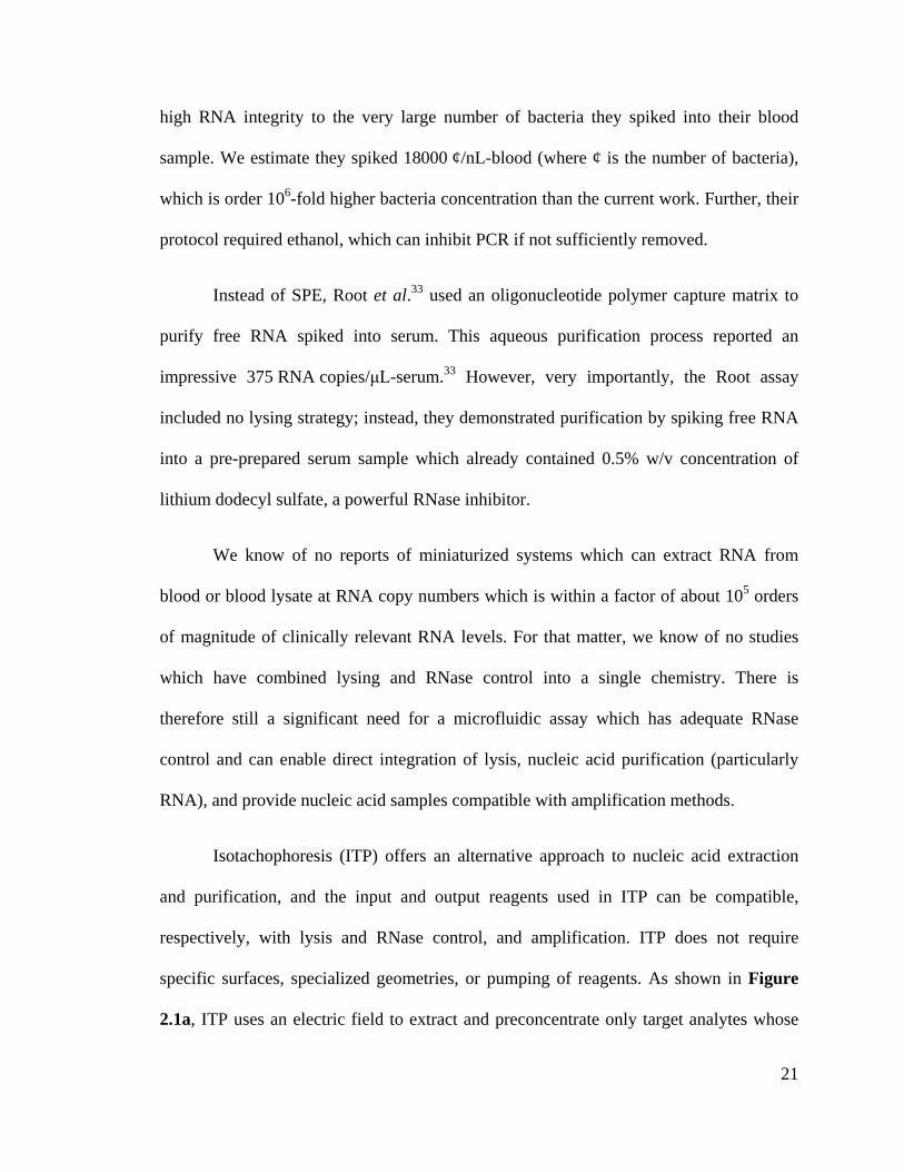
21

high RNA integrity to the very large number of bacteria they spiked into their blood

sample. We estimate they spiked 18000 ¢/nL-blood (where ¢ is the number of bacteria),

which is order 106-fold higher bacteria concentration than the current work. Further, their

protocol required ethanol, which can inhibit PCR if not sufficiently removed.

Instead of SPE, Root et al.33 used an oligonucleotide polymer capture matrix to

purify free RNA spiked into serum. This aqueous purification process reported an

impressive 375 RNA copies/μL-serum.33 However, very importantly, the Root assay

included no lysing strategy; instead, they demonstrated purification by spiking free RNA

into a pre-prepared serum sample which already contained 0.5% w/v concentration of

lithium dodecyl sulfate, a powerful RNase inhibitor.

We know of no reports of miniaturized systems which can extract RNA from

blood or blood lysate at RNA copy numbers which is within a factor of about 105 orders

of magnitude of clinically relevant RNA levels. For that matter, we know of no studies

which have combined lysing and RNase control into a single chemistry. There is

therefore still a significant need for a microfluidic assay which has adequate RNase

control and can enable direct integration of lysis, nucleic acid purification (particularly

RNA), and provide nucleic acid samples compatible with amplification methods.

Isotachophoresis (ITP) offers an alternative approach to nucleic acid extraction

and purification, and the input and output reagents used in ITP can be compatible,

respectively, with lysis and RNase control, and amplification. ITP does not require

specific surfaces, specialized geometries, or pumping of reagents. As shown in Figure

2.1a, ITP uses an electric field to extract and preconcentrate only target analytes whose

22

electrophoretic mobility is bracketed between the anions of its trailing (TE) and leading

electrolytes (LE). Anionic inhibitors with mobilites lower than of the TE do not focus,

but do electrophorese into the microchannel.

Figure 2.1 Schematic of the ITP-based NA purification from a complex biological sample such as blood

lysate. After dispensing the lysate containing TE into the well (top left of schematic and top channel), an

electric field was applied (middle channel), and the total NA migrated into the microchannel, where it was

focused and purified into the ITP interface. This process enables PCR inhibitors (including proteins) to

remain unfocused in the TE well (e.g., cations) or in channel regions well separated from the ITP zone.

After the total NA elutes into the LE well (bottom channel), the content was extracted using a standard

pipette. We then split this extract into two equal 4 ul aliquots for parallel off-chip RT-qPCR and qPCR

analyses.

The separation distance between these potentially PCR-inhibiting contaminants and the

focused nucleic acid in the ITP zone increases over time. For a channel length, L, the

separation distance between the ITP and the inhibitor zone front, L∆ , can be expressed as

( )LL TEi µµ−=∆ 1 , where iµ and TEµ are the inhibitor and TE anion mobilities,

23

respectively. For example, the zone front of an inhibitor with mobility TEi µµ 9.0= will

lag 0.6 cm behind the ITP zone at the end of our 6 cm microchannel. ITP is a highly

sensitive,96, 97 robust40, 98 sample preparation method which can, under ideal conditions,

provide up to one million-fold preconcentration.41 We have demonstrated successful ITP

extraction of small RNA from cell culture lysate;99 micro-RNA from total RNA;100, 101

genomic DNA (gDNA)102 and pathogenic DNA (malaria)103 from whole blood lysate; and

rRNA from bacteria in urine lysate.104 However, no previous nucleic acid extraction

protocols using ITP have been designed for adequate RNase control and RNA integrity.

2.2 Materials and methods

A schematic of our extraction process is shown in Figure 2.2. We started with human

whole blood infected with known concentrations of Pseudomonas Putida cells. We

chemically lysed the blood at room temperature for 1 min in a mixture of sodium

hydroxide (NaOH) (pH >12), Dithiothreitol (DTT) reducing agent, Triton X-100 non-

ionic surfactant, and synthetic carrier RNA. We then “quenched” this high pH with ice-

cold TE buffer, and then directly pipetted this combined lysate and TE into the input well

of a microfluidic chip with a single connecting channel (and single output well) pre-filled

with LE. We placed 600 μm diameter platinum wire electrodes into the wells, and applied

+1000 V to the extraction well and grounded the TE well using Keithley 2410

sourcemeter. We recorded current versus time using the sourcemeter interfaced with a

computer running a custom Matlab (Mathworks, Inc) script. As shown in Figure 2.4,

with constant voltage applied, the current monotonically decreased as the ITP zone

(containing the focused NA) advanced in the channel, and as the lower-conductivity

24

trailing electrolyte (TE) replaced the higher-conductivity leading electrolyte (LE). The

current signal plateaued near t = 220 s, coincident with the time at which the focused NA

eluted into the extraction well. With a standard pipette, we gently mixed the content of

the extraction well and collected 4 μl aliquots for each of the off-chip RT-qPCR and PCR

assays. In this study, we also performed SYBR Green based NA visualizations to

provide supporting evidence for the extracted and purified NA, however, the process can

be performed by monitoring current alone.

PSEUDOMONAS PUTIDA AND BLOOD SAMPLES: Blood samples from healthy

donors were collected in heparin tubes at the Stanford Blood Center. Aliquots of 100 μL

blood were prepared and stored at -80°C. Pseudomonas Putida cells were purchased from

ATCC (#12633), and cultured in Luria Broth (Invitrogen) at 37°C to a final concentration

of 3e6 ¢/mL, and quantified by the plate count method. Bacteria suspensions were

pelleted before diluting them in blood at 3x107, 3x106, 3x105, and 3x104 ¢/mL

concentrations, and were stored at -80°C.

LYSIS: We lysed 20 μL of whole blood with suspended P. putida using a mixture of 1%

Triton X-100, 125 mM NaOH, 40 mM DTT and 0.4 mg/mL carrier polyA RNA. After

1 min of incubation at room temperature, we mixed 10 μL of lysate with 90 μL of ice-

cold TE buffer (28 mM HEPES, 1% Triton X-100, pH~7.4).

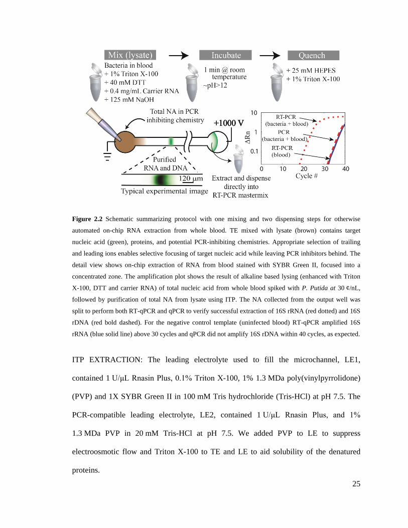
25

Figure 2.2 Schematic summarizing protocol with one mixing and two dispensing steps for otherwise

automated on-chip RNA extraction from whole blood. TE mixed with lysate (brown) contains target

nucleic acid (green), proteins, and potential PCR-inhibiting chemistries. Appropriate selection of trailing

and leading ions enables selective focusing of target nucleic acid while leaving PCR inhibitors behind. The

detail view shows on-chip extraction of RNA from blood stained with SYBR Green II, focused into a

concentrated zone. The amplification plot shows the result of alkaline based lysing (enhanced with Triton

X-100, DTT and carrier RNA) of total nucleic acid from whole blood spiked with P. Putida at 30 ¢/nL,

followed by purification of total NA from lysate using ITP. The NA collected from the output well was

split to perform both RT-qPCR and qPCR to verify successful extraction of 16S rRNA (red dotted) and 16S

rDNA (red bold dashed). For the negative control template (uninfected blood) RT-qPCR amplified 16S

rRNA (blue solid line) above 30 cycles and qPCR did not amplify 16S rDNA within 40 cycles, as expected.

ITP EXTRACTION: The leading electrolyte used to fill the microchannel, LE1,

contained 1 U/μL Rnasin Plus, 0.1% Triton X-100, 1% 1.3 MDa poly(vinylpyrrolidone)

(PVP) and 1X SYBR Green II in 100 mM Tris hydrochloride (Tris-HCl) at pH 7.5. The

PCR-compatible leading electrolyte, LE2, contained 1 U/μL Rnasin Plus, and 1%

1.3 MDa PVP in 20 mM Tris-HCl at pH 7.5. We added PVP to LE to suppress

electroosmotic flow and Triton X-100 to TE and LE to aid solubility of the denatured

proteins.

26

Triton X-100, NaOH, Tris, HEPES, and HCl were obtained from Sigma-Aldrich (St.

Louis, MO), DTT, carrier RNA, and SYBR Green II were obtained from Invitrogen

(Carlsbad, CA), PVP (MW 1.3 MDa) was purchased from ACROS Organics (Thermo

Fisher Scientific, NJ) and RNasin Plus was purchased from Promega (Madison, WI). All

solutions were prepared in UltraPure DNase/RNase free deionized (DI) water (GIBCO

Invitrogen, Carlsbad, CA).

CHANNEL PREPARATION: We performed isotachophoretic purification of RNA on a

60.7 mm long, 120 um wide, 35 um deep Crown glass microchannel (NS12A) interfaced

with 3.5 mm deep and 3.5 mm diameter wells from Caliper Science Life Sciences, CA.

Before first use, we rinsed the channel (Figure 2.3) with the following successive

washes: methanol (2 min), DI (1 min), 1 M HCl (2 min), DI (1 min), 1 M NaOH (10 min)

and DI (1 min). Between experiments, we rinsed the channel with 10% household bleach

for 2 min to remove any residual nucleic acid contaminants and then with washes of

1 min DI, 10 min NaOH and 1 min DI. To fill channel with LE1, we dispensed 10 μl of

LE1 into well 1, 2, and 3, and applied vacuum to well 4 for 1 min. We carefully emptied

well 1 and filled it with 10 μl of the PCR compatible LE2, and emptied, rinsed and filled

well 4 with 10 μl lysate containing TE. As the final step, we placed 600 μm diameter

platinum wire electrodes into the wells and applied 1000 V to initiate ITP. After the total

NA zone together with small amounts of TE anions eluted to well 1, we gently mixed the

content of this well and aspirated 4 μl for the RT-PCR and another 4 μl for the PCR

assays.

27

Figure 2.3 Microfluidic chip geometry. We performed isotachophoretic purification of NA on a L1-4 = 60.7

mm long, 120 um wide, 35 um deep Crown glass microchannel (NS12A) interfaced with 3.5 mm deep and

3.5 diameter wells from Caliper Science Life Sciences, CA. The wells sit open and exposed to room air

during ITP.

IMAGING SYSTEM: We performed on-chip visualizations using an inverted

epifluorescence microscope (Nikon Eclipse TE300) (Nikon, Tokyo, Japan) equipped with

a 10x objective (Plan, NA 0.30 (Nikon, Tokyo, Japan). A blue LED (Thor Labs, Newton,

NJ) was used for excitation of SYBR Green II (Invitrogen, Carlsbad, CA) nucleic acid

dye. We used a filter cube optimized for detection of FITC (FITC-A-Basic, Semrock,

Rochester, NY) and a 0.5x demagnification lens (Diagnostic Instruments, Sterling

Heights, MI). We captured images using 512x512, 16 bit, CCD camera (Cascade 512F,

QImaging/Photometrics, Canada). We controlled the camera using Winview32 (Princeton

Instruments, Trenton, NJ) and processed the images with MATLAB (R2007b,

Mathworks, Natick, MA).

TIMING: We recorded current over time using the sourcemeter interfaced with a

computer running a custom Matlab (Mathworks, Inc) script. As shown in Figure 2.4,

with constant voltage applied, the current monotonically decreased as the ITP zone

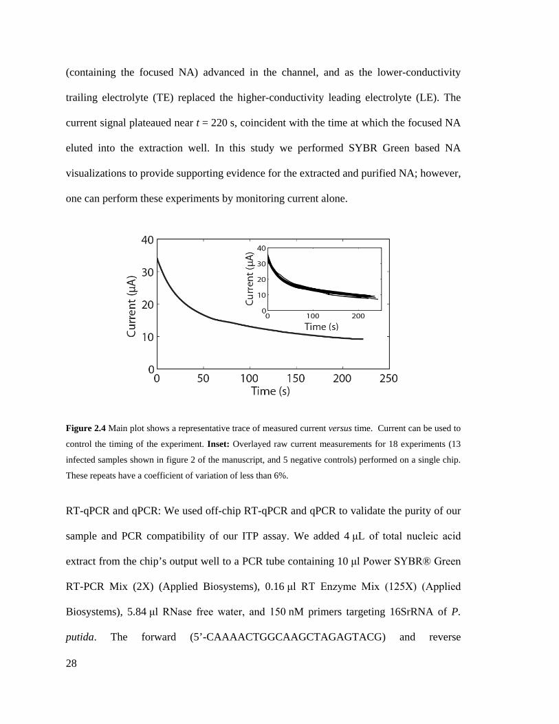
28

(containing the focused NA) advanced in the channel, and as the lower-conductivity

trailing electrolyte (TE) replaced the higher-conductivity leading electrolyte (LE). The

current signal plateaued near t = 220 s, coincident with the time at which the focused NA

eluted into the extraction well. In this study we performed SYBR Green based NA

visualizations to provide supporting evidence for the extracted and purified NA; however,

one can perform these experiments by monitoring current alone.

Figure 2.4 Main plot shows a representative trace of measured current versus time. Current can be used to

control the timing of the experiment. Inset: Overlayed raw current measurements for 18 experiments (13

infected samples shown in figure 2 of the manuscript, and 5 negative controls) performed on a single chip.

These repeats have a coefficient of variation of less than 6%.

RT-qPCR and qPCR: We used off-chip RT-qPCR and qPCR to validate the purity of our

sample and PCR compatibility of our ITP assay. We added 4 μL of total nucleic acid

extract from the chip’s output well to a PCR tube containing 10 μl Power SYBR® Green

RT-PCR Mix (2X) (Applied Biosystems), 0.16 μl RT Enzyme Mix (125X) (Applied

Biosystems), 5.84 μl RNase free water, and 150 nM primers targeting 16SrRNA of P.

putida. The forward (5’-CAAAACTGGCAAGCTAGAGTACG) and reverse

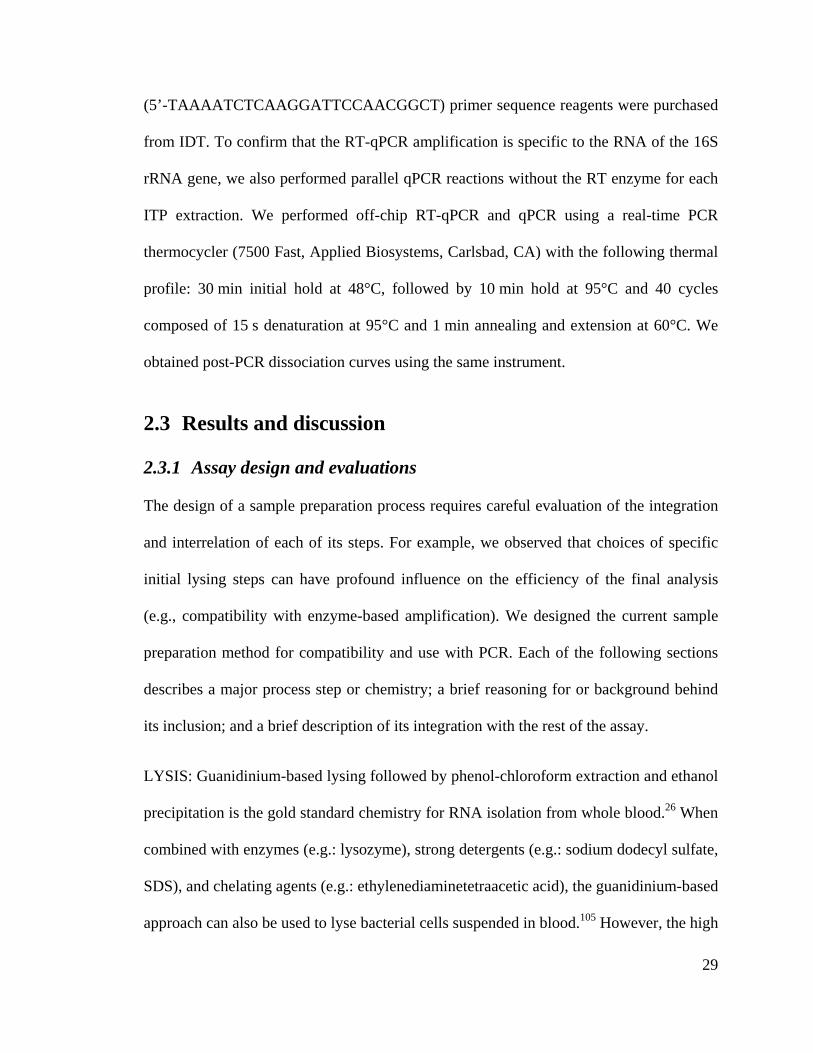
29

(5’-TAAAATCTCAAGGATTCCAACGGCT) primer sequence reagents were purchased

from IDT. To confirm that the RT-qPCR amplification is specific to the RNA of the 16S

rRNA gene, we also performed parallel qPCR reactions without the RT enzyme for each

ITP extraction. We performed off-chip RT-qPCR and qPCR using a real-time PCR

thermocycler (7500 Fast, Applied Biosystems, Carlsbad, CA) with the following thermal

profile: 30 min initial hold at 48°C, followed by 10 min hold at 95°C and 40 cycles

composed of 15 s denaturation at 95°C and 1 min annealing and extension at 60°C. We

obtained post-PCR dissociation curves using the same instrument.

2.3 Results and discussion

2.3.1 Assay design and evaluations

The design of a sample preparation process requires careful evaluation of the integration

and interrelation of each of its steps. For example, we observed that choices of specific

initial lysing steps can have profound influence on the efficiency of the final analysis

(e.g., compatibility with enzyme-based amplification). We designed the current sample

preparation method for compatibility and use with PCR. Each of the following sections

describes a major process step or chemistry; a brief reasoning for or background behind

its inclusion; and a brief description of its integration with the rest of the assay.

LYSIS: Guanidinium-based lysing followed by phenol-chloroform extraction and ethanol

precipitation is the gold standard chemistry for RNA isolation from whole blood.26 When

combined with enzymes (e.g.: lysozyme), strong detergents (e.g.: sodium dodecyl sulfate,

SDS), and chelating agents (e.g.: ethylenediaminetetraacetic acid), the guanidinium-based

approach can also be used to lyse bacterial cells suspended in blood.105 However, the high

30

ionic strengths (e.g. >500 mM) of these mixtures require careful purification including

wash and buffer exchanges as SDS, chaotropic agents, organic solvents, and alcohols are

strong PCR inhibitors. We rejected these here because high ionic strength (especially

when including high mobility anions) can be challenging to integrate with ITP. Instead,

we opted for alkali-based lysis. The alkali approach is widely used for isolation of

plasmid DNA from bacterial cells,106 but it is not commonly applied for RNA isolation,

likely due to the instability of RNA at high pH.107 While incubation in NaOH may

contribute to some RNA degradation, we found it had negligible effect on RT-qPCR

amplification of our target RNA sequences. For example, in a set of preliminary

experiments (data not shown), we found negligible differences in RT-qPCR threshold

cycle for samples of pre-purified (using a standard SPE column, PureLink RNA Mini kit

from Life Technologies Corp., Carlsbad, CA) 16S rRNA with and without treatment with

125 mM NaOH for 1 min. With respect to lysing, we found (again, through preliminary

repeated trials and lysing quantitation studies) that this 1 min incubation (required to

protect RNA) showed lysing performance on par with even 5 min of 130 mM NaOH or

higher concentration (data not shown).

RNASE CONTROL: RNA is easily hydrolyzed at elevated temperature, and at either

alkali or acidic conditions. Further, its stability is significantly compromised by the

abundance of ribonucleases (RNases) in blood. Tsui et al. showed that free RNA can no

longer be amplified after incubation in blood plasma for 15 s!12 RNase activity requires

its disulfide (S-S) bond be intact. While NaOH can reduce these S-S bonds, the half-life

of RNase in 0.2 M NaOH is ~30 min.108 Meanwhile, as we have mentioned, long

incubation in alkali conditions degrades RNA. However, RNase degradation can be

31

greatly accelerated during alkali lysing by adding detergents (e.g., SDS), and/or reducing

agents (e.g., DTT).109 While ITP can be compatible with anionic detergents, we found

that the addition of a reducing agent alone, 40 mM DTT to 125 mM NaOH in the

presence of 1% non-ionic detergent (Triton X-100), results in adequate mitigation of

RNA degradation in our assay. We hypothesize that this mixture adequately destabilizes

and covalently destroys disulfide bonds of the normally very stable RNases even during 1

min of incubation.

After the lysate is quenched to normal pH, residual RNase may be present. To inhibit the

activity of the remaining ribonucleases, we explored the use of formamide as the solvent

for the lysate and TE. While pure formamide stabilizes RNA in the presence of RNase,110

we found (again through preliminary work) that a combination of 50% formamide and

20% blood unfortunately resulted in enhanced RNA degradation. Similar observations

were reported by Strauss and Sinsheimer111 in an evaluation of initial kinetics of RNA

degradation by pancreatic ribonucleases. Instead of formamide, we opted for an indirect

approach: the addition of carrier RNA. The term ‘carrier RNA’ refers to exogenous RNA

spiked into a sample.112 Addition of carrier RNA to lysate reportedly enhances the

recovery of low traces of DNA and RNA in ethanol precipitation113, 114 and SPE-based

extraction35, 115 procedures. In our application, we spiked large amounts of polyA

synthetic carrier RNA sequences into the lysate to serve as a competitive substrate for

RNase activity. That is, we hypothesize that the abundant carrier RNA reduces enzymatic

activity on our trace-concentration, target RNA by acting as a high abundance inhibitor to

RNase. Figure 2.5 summarizes example preliminary experiments we performed in part to

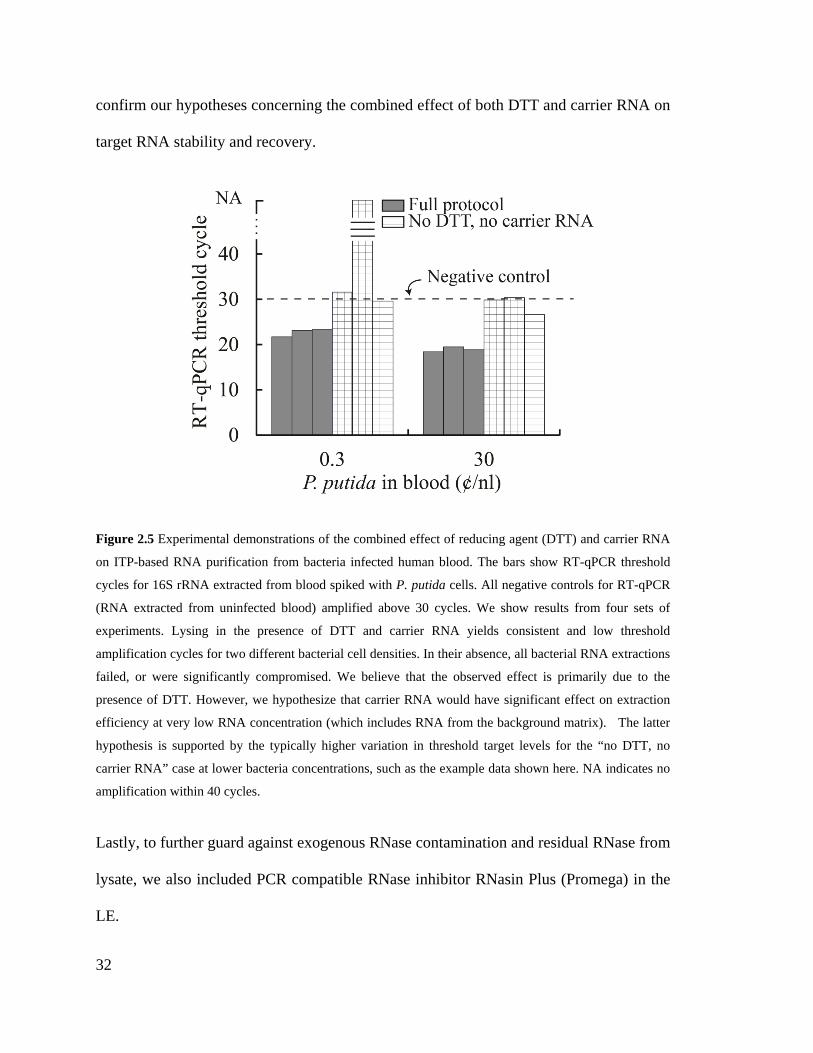
32

confirm our hypotheses concerning the combined effect of both DTT and carrier RNA on

target RNA stability and recovery.

Figure 2.5 Experimental demonstrations of the combined effect of reducing agent (DTT) and carrier RNA

on ITP-based RNA purification from bacteria infected human blood. The bars show RT-qPCR threshold

cycles for 16S rRNA extracted from blood spiked with P. putida cells. All negative controls for RT-qPCR

(RNA extracted from uninfected blood) amplified above 30 cycles. We show results from four sets of

experiments. Lysing in the presence of DTT and carrier RNA yields consistent and low threshold

amplification cycles for two different bacterial cell densities. In their absence, all bacterial RNA extractions

failed, or were significantly compromised. We believe that the observed effect is primarily due to the

presence of DTT. However, we hypothesize that carrier RNA would have significant effect on extraction

efficiency at very low RNA concentration (which includes RNA from the background matrix). The latter

hypothesis is supported by the typically higher variation in threshold target levels for the “no DTT, no

carrier RNA” case at lower bacteria concentrations, such as the example data shown here. NA indicates no

amplification within 40 cycles.

Lastly, to further guard against exogenous RNase contamination and residual RNase from

lysate, we also included PCR compatible RNase inhibitor RNasin Plus (Promega) in the

LE.

33

ITP CHEMISTRY: In addition to requiring TE and LE anions with mobilities which

bracket that of RNA, the ITP chemistry prompted two additional concerns: pH and ionic

strength. Again, throughout the course of a series of preliminary experiments, we

observed severe repeatability problems at lower pH 5-7 (e.g., using Bis-Tris as the

buffering weak base). We attribute these to the effects of (observed) protein aggregation

and protein adsorption to channel walls.116, 117 Recovery efficiency stabilized at pH ~7.5,

and so we chose Tris as the buffering counterion. We also quantified LE buffer

compatibility with RT-PCR (via independent, ex situ runs with the PCR system) and

found no change in the amplification efficiency when using 20 mM Tris-HCl (pH = 7.5)

as the sample buffer added to the RT-PCR mastermix. We filled the channel with

100 mM Tris-HCl (pH = 7.5) to improve the rate of nucleic acid accumulation42 but used

20 mM Tris-HCl (pH = 7.5) as the LE buffer in the extraction well. The latter chemistry

provided a good balance between PCR compatibility and buffering capacity in that well.

2.3.2 Demonstration of extraction purity and compatibility with RT-qPCR

FLOURESCENCE IMAGING: We monitored accumulation of RNA during ITP by

visualizing the scalar fluorescence of RNA specific-intercalating dye, SYBR Green II.

Figure 2.6 illustrates results of extractions from blood containing 0 and 30 ¢/nL P. putida

cells. Our 1X concentration of SYBR Green II (in original LE1; equivalent to 0.003X

concentration in the final PCR mix) showed no observable effect on amplification signal.

34

Figure 2.6 Example on-chip fluorescence images and experimental integrated fluorescence curves of

extracted nucleic acid ITP zones stained with SYBR Green II. The inset fluorescence profile and image on

the top right shows RNA extracted from uninfected blood (negative control). The main fluorescence plot

and image at the bottom corresponds to a typical run with blood infected with P. putida at 30 ¢/nL

concentration. We corrected the ITP-focused nucleic acid fluorescence images by subtracting a background

fluorescence image and dividing this by the difference between a flat field image and the background

image (see the supplementary information document of Persat et al. for further details). For the

fluorescence peak distribution, we integrated image intensities along the width of the channel and show

here versus distance along the channel’s main axis. These image analysis and fluorescence integrations

were performed using MATLAB (The Mathworks, MA).

RT-qPCR AND qPCR: Figure 2.7 shows typical RT-qPCR threshold cycles for 16S

rRNA extracted from P. putida suspended in whole human blood. We explored bacterial

cell densities ranging four orders of magnitude from 0.03 to 30 ¢/nL.

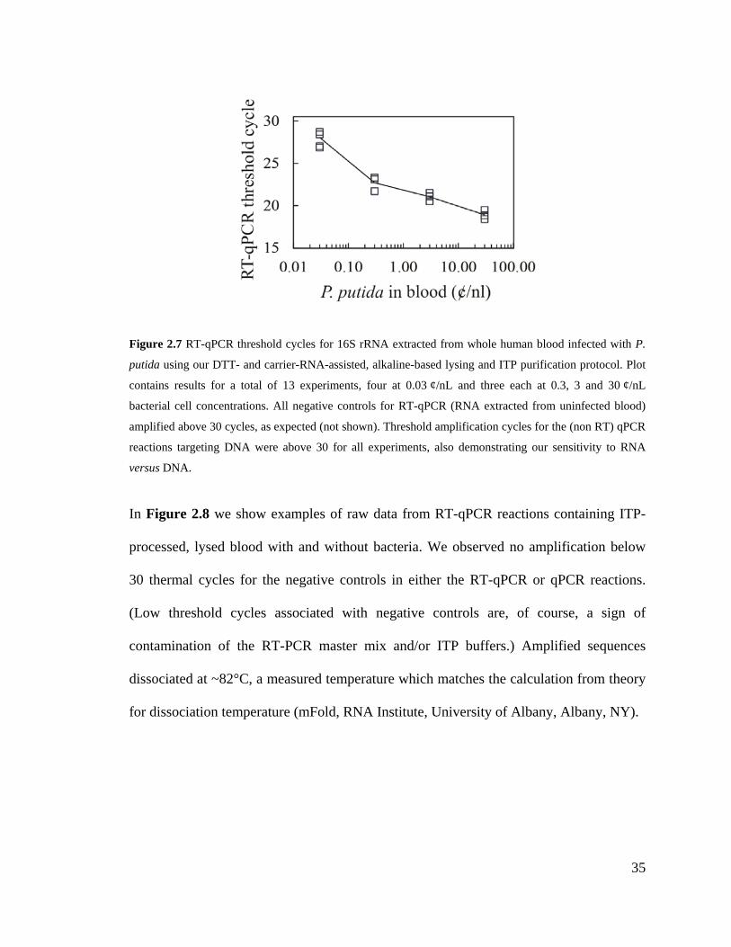
35

Figure 2.7 RT-qPCR threshold cycles for 16S rRNA extracted from whole human blood infected with P.

putida using our DTT- and carrier-RNA-assisted, alkaline-based lysing and ITP purification protocol. Plot

contains results for a total of 13 experiments, four at 0.03 ¢/nL and three each at 0.3, 3 and 30 ¢/nL

bacterial cell concentrations. All negative controls for RT-qPCR (RNA extracted from uninfected blood)

amplified above 30 cycles, as expected (not shown). Threshold amplification cycles for the (non RT) qPCR

reactions targeting DNA were above 30 for all experiments, also demonstrating our sensitivity to RNA

versus DNA.

In Figure 2.8 we show examples of raw data from RT-qPCR reactions containing ITP-

processed, lysed blood with and without bacteria. We observed no amplification below

30 thermal cycles for the negative controls in either the RT-qPCR or qPCR reactions.

(Low threshold cycles associated with negative controls are, of course, a sign of

contamination of the RT-PCR master mix and/or ITP buffers.) Amplified sequences

dissociated at ~82°C, a measured temperature which matches the calculation from theory

for dissociation temperature (mFold, RNA Institute, University of Albany, Albany, NY).

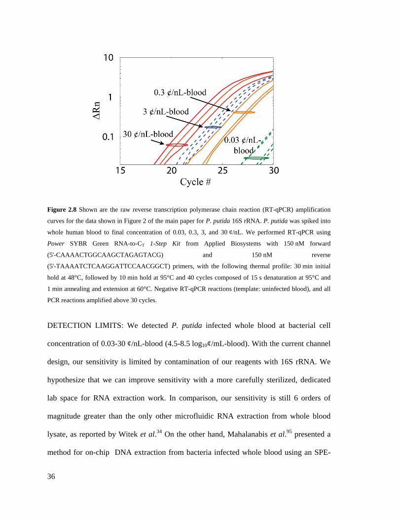
36

Figure 2.8 Shown are the raw reverse transcription polymerase chain reaction (RT-qPCR) amplification

curves for the data shown in Figure 2 of the main paper for P. putida 16S rRNA. P. putida was spiked into

whole human blood to final concentration of 0.03, 0.3, 3, and 30 ¢/nL. We performed RT-qPCR using

Power SYBR Green RNA-to-CT 1-Step Kit from Applied Biosystems with 150 nM forward

(5'-CAAAACTGGCAAGCTAGAGTACG) and 150 nM reverse

(5'-TAAAATCTCAAGGATTCCAACGGCT) primers, with the following thermal profile: 30 min initial

hold at 48°C, followed by 10 min hold at 95°C and 40 cycles composed of 15 s denaturation at 95°C and

1 min annealing and extension at 60°C. Negative RT-qPCR reactions (template: uninfected blood), and all

PCR reactions amplified above 30 cycles.

DETECTION LIMITS: We detected P. putida infected whole blood at bacterial cell

concentration of 0.03-30 ¢/nL-blood (4.5-8.5 log10¢/mL-blood). With the current channel

design, our sensitivity is limited by contamination of our reagents with 16S rRNA. We

hypothesize that we can improve sensitivity with a more carefully sterilized, dedicated

lab space for RNA extraction work. In comparison, our sensitivity is still 6 orders of

magnitude greater than the only other microfluidic RNA extraction from whole blood

lysate, as reported by Witek et al.34 On the other hand, Mahalanabis et al.95 presented a

method for on-chip DNA extraction from bacteria infected whole blood using an SPE-

37

based extraction method which processed about 100 μl of whole blood using a protocol

with five reagent pumping steps, and which achieved 102 ¢/mL sensitivity. This

sensitivity is order 300 fold higher than our assay, but used about 5 orders of magnitude

higher processed sample volume than our assay’s ~1 nL processed volume. We

hypothesize that we can exceed this sensitivity by scaling up the geometry of our channel

to process order 1000 fold higher sample volume (order ~1 µl), and hope to demonstrate

this in future work.

In addition to the P. putida results we present here, we have also successfully performed

RNA extraction from E. coli cells suspended in whole blood (data not shown). Together,

our more extensive P. putida work and our limited work with E. coli suggest that our

protocol can be successfully adapted to RNA extraction and detection from many gram-

negative bacteria species by simply changing the primer sequence and thermal cycling

conditions for RT-qPCR. One particular application that may benefit from our technique

is diagnosis of Menigococcemia, an acute and potentially life-threatening infection of the

bloodstream caused by bacteria Neisseria meningitidis. One large study including 1045

adult patients evaluated the full range bacterial loads upon hospital admission, 2.87 –

6.3 log10¢/mL,118 using qPCR analysis of whole blood samples for N. meningitides.

Another study, including a smaller cohort of 51 pediatric patients reported a slightly

higher N. meningitides load range of 4.3 - 8.2 log10¢/mL119 using a similar qPCR-based

assay.

38

3 Temperature Effects on Electrophoresis

The contents of this chapter were previously published by Rogacs and Santiago (2013)120

and are reproduces here with minor modifications.

3.1 Introduction

The fields of drug discovery, genetics, proteomics, toxin detection, and food

analysis, among others, employ electrophoretic separation as a workhorse analysis

technique. Electrophoresis methods include capillary electrophoresis (CE),

isotachophoresis (ITP), isoelectric focusing (IEF) and temperature gradient focusing

(TGF); all of which rely on differences between analyte electrophoretic mobilities for

separation.53 A wide range of these methods use temperature variation to improve

performance and enable new functionalities. Likely the most common utility of elevated

temperature is speeding up electrophoretic separations.50-52 For example, compared to

room temperature, CE separation times can be reduced by 2.5-fold at 70°C.52, 53 Other

uses include improvement of resolution by changing the degree of ionization of

analytes,121-127 and manipulation of nucleic acid secondary structure52, 128 or protein

conformation.129, 130 TGF specifically relies on temperature gradients to focus and

separate analytes.131, 132 Temperature effects on electrophoresis can also cause non-ideal

behavior, including experimental variability, Joule-heating-induced zone dispersion,54, 56,

57 and increased electromigration dispersion.59, 133 As we will discuss, a 5°C temperature

change can produce as much as 0.1 units change in the pH, and over 25% change in

observable mobility of analytes at specific conditions.

39

The observable mobility of an ion depends on the solvent viscosity, ionic strength

of the electrolyte solution, the degree of ionization of the ion, and solvation of the ion.

The temperature sensitivity of viscosity, varying 2% per °C near room temperature,49 has

a marked influence on electrophoretic mobility, and is typically modeled using the so-

called Walden’s rule. Similarly, the strong temperature dependence of ion dissociation

constant (K) can have pronounced influence on the degree of ionization and so the

observable mobility of an ion. We here refer to only acid dissociation constants, Ka and

never the related base equilibrium constants, aWa KKK = , so we drop the ‘‘a’’ with no

ambiguity.) As we shall discuss, neglecting this effect can result in gross errors in

prediction for buffer pH (e.g., greater than 0.5 pH unit), buffer conductivity (>100%) and

effective mobility of analytes (>400%) at 80°C (all relative to room temperature, see

Supporting Information for details). Although commonly used, Walden’s rule does not

hold for some small ions like potassium or chloride, which are poorly hydrated at low

temperatures. Neglecting temperature dependence of hydration shell for small ions (e.g.,

K+ or Cl-) can result in as much as ~20% error in the predicted absolute mobilities over a

70°C change.134

In general, the contributions to electrophoretic mobility from temperature

dependence of electrolyte ionization, ionic strength corrections, and ion solvation, have

been largely overlooked.135 In Table 3.1, we show the results of a brief survey of

temperature effects addressed by published models, and compare these to the current

work. Most of these studies explored temperature effects on one of two types of

electrolyte properties, but not on both. These two types are (1) weak electrolyte pK, (e.g.,

Okamoto et al.136) and (2) the ‘actual’ mobility of fully ionized electrolytes. (e.g.,

40

Anderko and Lencka137) In Table 3.1, we indicate with a dash if temperature effects on

an electrolyte property were not considered in (or if property was not relevant to) the

study. Despite the importance and prevalence of the various effects, we found no

comprehensive models which capture all important contributors of temperature to ion

(weak and strong electrolyte) mobilities and electrolyte solution conductivity and pH. For

example, we know of no studies of temperature effects on electrolyte properties which

capture both solvation effects and dissociation effects, nor models including ionic

strength corrections to both pK and absolute mobility.

Table 3.1 Examples of temperature models of aqueous electrolyte solutions from the last 25 years. Effects

captured by each model are categorized into two types: pK or actual mobility, μo corrections. Abbreviation

‘dpK/dT’ indicates that only tabulated values of this slope were presented. ‘pKC-VC’ and ‘pKC-CG’

represent models which account for temperature dependence of pK using van’t Hoff or the higher accuracy

Clark-Glew model, respectively. Viscosity corrections using of the Walden rule type are indicated with

‘W’. We also list models which account for the temperature dependence of ionic strength corrections of

activity coefficient (‘ISC-pK’) and actual mobility (‘ISC-μ’).

References Acid dissociation constant, pK(T)

Actual mobility, μ°(T)

Clancy (1987)138 dpK/dT, ISC-pK - Rush et al. (1991)129 - W Whang and Yeung (1992)126 dpK/dT W Chang and Yeung (1993)127 dpK/dT W Beynon and Easterby (1996)139 dpK/dT - Okamoto et al. (1997)136 pKC-VH, ISC-pK - Anderko and Lencka (1997)137 - W, ISC-μ, SSC Fukada and Takahashi (1998)140 pKC-VH, pKC-CG -

Rochu et al. (1999)130 - W Wang and Tsao (2004)141 - W Reijenga et al. (2007)142 dpK/dT W Evenhuis et al. (2007)135 - W, ISC-μ Mandaji et al. (2009)143 dpK/dT W Milanova et al. (2011)144 - W Current work pKC-VH, pKC-CG, ISC-pK W, ISC-μ, SSC

41

A fully comprehensive model for temperature effects on electrophoretic mobility

is challenging as temperature change may lead to ad hoc and difficult-to-predict effects

including variations in DNA gel migration dynamics,145 sieving matrix properties,146 and

electroosmotic flow (EOF).147 However, the basic phenomena associated with the

mobility of weak electrolyte ions in water and the electrolyte solution pH are addressable

using a fairly general model. These basic phenomena can be used to directly predict

temperature-dependence of electrolyte solution pH and conductivity, and analyte

mobility; likely the most relevant parameters in any separation assay.

We here present a fairly comprehensive model to quantify the effects of

temperature on analyte mobility and solution conductivity. Our model includes

temperature dependence of (1) viscosity, (2) ionic strength corrections on both mobility

and pK, (3) degree of ionization (pK), and (4) ion solvation effects on mobility. Our

model leverages thermophysical data for water viscosity;49 temperature dependence of

the Onsager-Fuoss model for finite ionic strength effects on mobility;148, 149 temperature

dependence of the extended Debye-Huckel theory for correction of ionic activity;149, 150

the Clarke-Glew generalized approach151 to predict K(T) from tabulated thermodynamic

properties;152 and species-specific, empirically evaluated correction terms for

temperature-dependence of Stokes’ radii of 11 common small ions.134 We validated our

model using a series of conductance and pH measurements across a temperature variation

of 25°C to 70°C for a set of electrolyte solutions routinely used in electrophoresis.

42

3.2 Theory

We define the mobility of species i, iµ , as the drift velocity of the ion through the

solvent divided by the applied electric field magnitude, E. As usual, we define the

‘limiting’ (or absolute) mobility of an ion in solution as the mobility that a fully ionized

ion would take in the limit of infinite dilution and with known integer values of its

valence. At finite ionic strength, the ‘actual’ mobility of an ion is obtained by considering

the effect of the ionic atmosphere on the movement of the fully ionized ion.66 For weak

electrolytes, the observed or ‘effective’ electrophoretic mobilities are dependent on the

degree of dissociation of the analyte. We here summarize the models describing the

temperature effect on limiting, actual, and effective ionic mobilites. These include

temperate dependent variations of viscosity, dielectric constant, ion solvation, ionic

strength effects, and dissociation constants.

3.2.1 Walden’s rule

The limiting mobility, oiµ , of ionic species i, can be formulated as a balance

between the applied electric force and retarding frictional forces acting on the ion. For

infinite dilution, this balance can be approximately modeled by a form of Stokes’ drag

law as follows:

𝜇𝑖0 =𝑧𝑖𝑒

6𝜋𝜂𝑟𝑠,𝑖. (3.1)

Here zi is the valence of the ion, e is the elementary charge (electron charge), η is the

dynamic viscosity of the solvent, and rs,i is the Stokes’ (or hydrodynamic) radius of the

solvated ion. Stokes’ law describes the drag on a sphere in a simple, continuum fluid

43

flow in the limit of negligible inertial effects. The Stokes’s radius of an ion can be

interpreted as the radius of a sphere with the same viscous drag as the ion. Because of

non-continuum effects and the complex interactions between the ion, nearby counterions,

and the solvent molecules, the Stokes’ radius is only roughly related to other measures of

ion dimensions such as the crystallographic radius. Even in the limit of infinite dilution,

the Stokes’ radius of an ion is therefore an empirically determined quantity which

accounts for the non-spherical nature of the ion and the effect of its hydration shell. This

quantity is often measured at some reference temperature,θ .

Treatment of limiting ion mobility as a balance between electric force and a drag

law from continuum flow theory leads to an approximate relation between mobility and

solvent viscosity. For aqueous solutions, we can leverage empirical correlations for

water viscosity, η, as a function of temperature, T, as follows:49

𝑙𝑜𝑔10 �𝜇(𝑇)

𝜇(20℃)� =20 − 𝑇𝑇 + 96

{1.2378 − 1.303 × 10−3(20 − 𝑇)

+3.06 × 10−6(20 − 𝑇)2 + 2.55 × 10−8(20 − 𝑇)3}.

(3.2)

This useful correlation covers the temperature range of -8°C ≤ T ≤ 150°C with an

uncertainty of ±0.26%. Equation (3.1) suggests that a change in the viscosity of the

medium will lead to an approximately inversely proportionate change in the limiting

mobility of the ion. This leads to the definition of the Walden’s rule or Walden’s

product, oziiWP ,ηµ= .153 Walden’s rule assumes iWP is independent of temperature for

each ion and can be used to correct the limiting mobility of ions, ozi,µ , evaluated at the

reference temperature, θ , as follows:

44

𝜇𝑖,𝑧0 (𝑇) = 𝛼𝜇𝑖,𝑧0 (𝜃), (3.3)

where ( ) ( )Tηθηα /= . (We will use “T” in parentheses periodically to emphasize the

temperature dependence of a variable.) Walden’s rule is useful in gaining physical

intuition into solvent viscosity effects on limiting ion mobility. However, as we discuss

below, application of Walden’s rule alone to predict ion mobility can result in severely

erroneous mobility predictions at a given operating temperature, T.

3.2.2 Ion solvation effect on limiting ion mobility

As we have mentioned, the idea of a Stokes’ radius and Walden’s rule in

determining limiting ion mobility has only limited use. Quantitatively, the Walden

product in Eq. (3.3) is known to vary with temperature, particularly for small ions. This

inaccuracy is due to the complexity of ion-solvent interactions which is only

approximately captured by a continuum drag law in terms of solvent viscosity. We here

present a summary discussion of the physicochemical nature of these interactions and

then propose a set of empirical corrections for prediction of limiting ion mobilities for

common small ions. We incorporate these empirical corrections in our model. E.R.

Nightingale (1959) studied and showed the importance of ion-solvent interactions in the

prediction of limiting ion mobility. Nightingale134 provided empirical data for the

Walden product (in water) of varying Stokes radii as a function of temperature. The data

show that this temperature dependence is highly specific to ions. The typical trend is for

Walden product, WP, to decrease with increasing temperature, and the effect is most

pronounced for smaller ions such as chloride, potassium, and nitrate. Nightingale

qualitatively attributed this effect to the ion-dependent disruption of water structure for

45

ions of varying size and shape. A review of such empirical data for limiting ion mobility

and the theory behind solvent-ion interactions was presented by Sadek.154 Sadek

similarly described these phenomena in the context of ‘structure making’ or ‘structure

breaking’ properties of ions and the solvent. Water possesses quartz-like molecular

structure, a tethrahedral coordination, in which each water molecule can participate in

two collective hydrogen bonds. This permits the existence of cavities of various sizes.

Sadek classified ions into three categories associated with the relative size of the ions

versus the size of these cavities in the water structure. These hypotheses propose that the

small ions occupy these cavities in the water, and the relative size of the ion and the

cavity helps determine the degree of order in the hydration shell around the ion. Stokes’

type law is most useful and accurate for ions whose size is relatively large compared to

the dimensions of these cavities.

The current theories of ion solvation are useful in providing intuition as to the ion-

specific nature of temperature dependence of limiting mobility. However, despite

significant work in the field,154 a theory for quantitative prediction of these effects is not

available. Indeed, the physicochemical nature of ion-solvent interactions is not well

understood, and considered one of the most difficult problems associated with the study

of electrolyte solutions.154-156 We here therefore take the approach of providing ion-

specific empirical corrections for the effect of solvation on limiting ion mobility. To this

end, we exploit the clear trend in the data that the smallest ions are subject to the

strongest temperature dependence of limiting ion mobility (and WP). We formulate this

correction in terms of empirical data for temperature dependence of the ion-specific,

valence-normalized Walden’s product, ioo

ii zWP ηλ= , expressed in terms of the limiting

46

conductivity, oiλ , for 11 species,134 where limiting ionic equivalent conductance is

defined as ( )osi

oi rz ηλ ,820.0= . Here, we define the solvation correction term for ion i as

( ) ( )( ) ( ) ( )( )θηθληλβ ooi

ooii TT≡ , which we use to correct for ion-solvation associated

temperature effects on limiting mobility. At the operating temperature, T, we therefore

evaluate the limiting mobility as

𝜇𝑖,𝑧0 (𝑇) = 𝛼𝛽𝑖𝜇𝑖,𝑧0 (𝜃), (3.4)

where ( )θµ ozi, is the limiting mobility of an ion measured at the reference temperature, θ,

and α accounts for the inversely proportionate change in the limiting mobility of the ion

with viscosity. The 11 cases for which we provide the temperature-dependent correction

term, βi include chloride, sodium, potassium, nitrate, lithium, magnesium, perchlorate,

rubidium, cesium, calcium, silver, and sulfate. Chloride, potassium, perchlorate, and

nitrate particularly exhibit strong temperature dependence and are also common

electrolyte ions. Our experimental validation of our model shows that neglecting these

ion solvation corrections can result in as much as 20% error in prediction of ion

mobilities (e.g., for the case of K+ over a 70°C change).

3.2.3 Ionic strength correction of limiting mobility: actual ion mobility

So far, we have discussed ion mobilities for the case of fully-ionized ions at infinitesimal

ionic strength. At finite ionic strength, the presence of an ionic atmosphere around the ion

reduces (in all cases) the limiting ion mobility to the so-called actual mobility. There is a

wide body of accepted quantitative theory describing these phenomena.66 Here, we adopt

47

the extended Onsager-Fuoss model, which is applicable to an arbitrary mixture of species

at ionic strengths up to 100 mM,157 and can be formulated as follows:

𝜇𝑖,𝑧(𝑇) = 𝛼𝛽𝑖𝜇𝑖,𝑧0 (𝜃) − �𝐴𝛼𝛽𝑖𝜇𝑖,𝑧0 (𝜃) + 𝐵�√𝛤

1 + 𝑎𝐷√2

√𝛤, (3.5)

where

𝛤 = �� 𝑧2𝑐𝑖,𝑧

𝑝𝑖

𝑧=𝑛𝑖

𝑠

𝑖=1

.

Here, s is the number of species, zi is the charge number of the i-th ionic species, ε the

permittivity of solution, k is the Boltzmann constant, e is the elementary charge, NAV is

the Avogadro constant, T is the temperature of the solution and Γ is twice ionic strength,

I. The coefficients Cn and the vectors Rn are given by Onsager and Fuoss.148

We note our formulation of the extended Onsager-Fuoss differs from previous versions

(e.g., as used by Bahga and Santiago66) in employing the pre-factors α and βi to account

for temperature effects. Recall, the temperature-dependent term, α, accounts for the

inversely proportionate change in the limiting mobility of the ion with viscosity; and βi, is

a modification of Onsager-Fuoss model which we propose here to correct for ion

solvation effects.

We use a standard approach to account for the ionic-strength-related reduction in

mobility. This reduction can be attributed primarily to two factors. The first is

represented by the temperature dependent term, A. This is the so-called relaxation effect

which captures the polarization of the ionic atmosphere surrounding the ion, which acts

48

to lower the effective, local electric field experienced by the ion. By definition, the

absolute temperature appears in parameter A, which is defined as

𝐴 = 𝑧𝑖𝑒3

12𝜋�

𝑁𝐴𝑉(𝜀𝑘𝑇)3�𝐶𝑛𝑅𝑖𝑛

∞

𝑛=0

, (3.6)

where ε is the water dielectric constant, whose temperature dependence can be

approximated by the following empirical correlation:103

𝜀 = 249.21 − 0.79069𝑇 + (0.72997 × 10−3)𝑇2. (3.7)

A depends on temperature as, ( ) 231 Tε , a fairly weak temperature dependence.

The second effect associated with ionic strength reduction of mobility is captured by the

parameter B. This is the so-called electrophoretic effect which is associated with the drag

force exerted by the moving counter-ion cloud on the central ion. Water viscosity and

dielectric constant each impact the magnitude of this drag force, formulated as

𝐵 = |𝑧𝑖|𝑒2

6𝜋𝜂�𝑁𝐴𝑉𝜀𝑘𝑇

, (3.8)

which makes B a strong function of temperature.

The aD term in the extended Onsager-Fuoss model takes into account the finite size of

ions, where a represents the mean distance of the closest approach for the ions (distance

from center of the central ion to the start of the ionic atmosphere).148, 158 The value

assigned to aD is empirically determined, and estimated to lie between 1 and 2 dm3/2 mol-

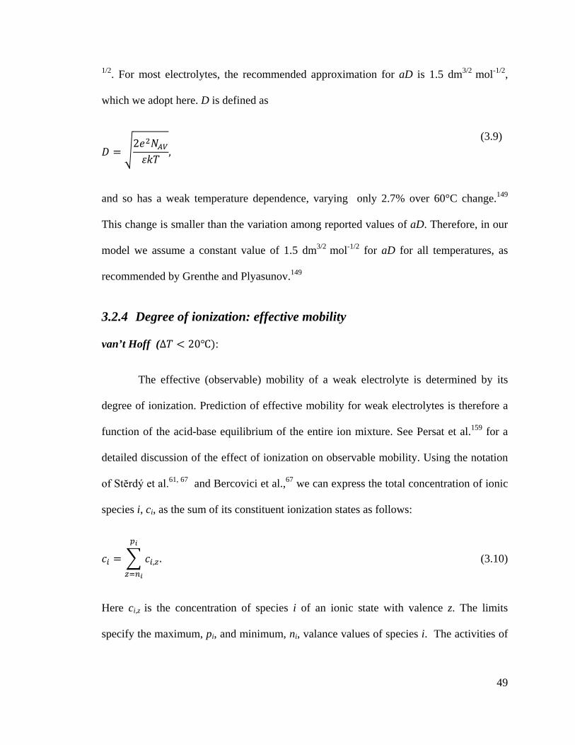
49

1/2. For most electrolytes, the recommended approximation for aD is 1.5 dm3/2 mol-1/2,

which we adopt here. D is defined as

𝐷 = �2𝑒2𝑁𝐴𝑉𝜀𝑘𝑇

, (3.9)

and so has a weak temperature dependence, varying only 2.7% over 60°C change.149

This change is smaller than the variation among reported values of aD. Therefore, in our

model we assume a constant value of 1.5 dm3/2 mol-1/2 for aD for all temperatures, as

recommended by Grenthe and Plyasunov.149

3.2.4 Degree of ionization: effective mobility

van’t Hoff (Δ𝑇 < 20℃):

The effective (observable) mobility of a weak electrolyte is determined by its

degree of ionization. Prediction of effective mobility for weak electrolytes is therefore a

function of the acid-base equilibrium of the entire ion mixture. See Persat et al.159 for a

detailed discussion of the effect of ionization on observable mobility. Using the notation

of Stĕrdý et al.61, 67 and Bercovici et al.,67 we can express the total concentration of ionic

species i, ci, as the sum of its constituent ionization states as follows:

𝑐𝑖 = � 𝑐𝑖,𝑧

𝑝𝑖

𝑧=𝑛𝑖

. (3.10)

Here ci,z is the concentration of species i of an ionic state with valence z. The limits

specify the maximum, pi, and minimum, ni, valance values of species i. The activities of

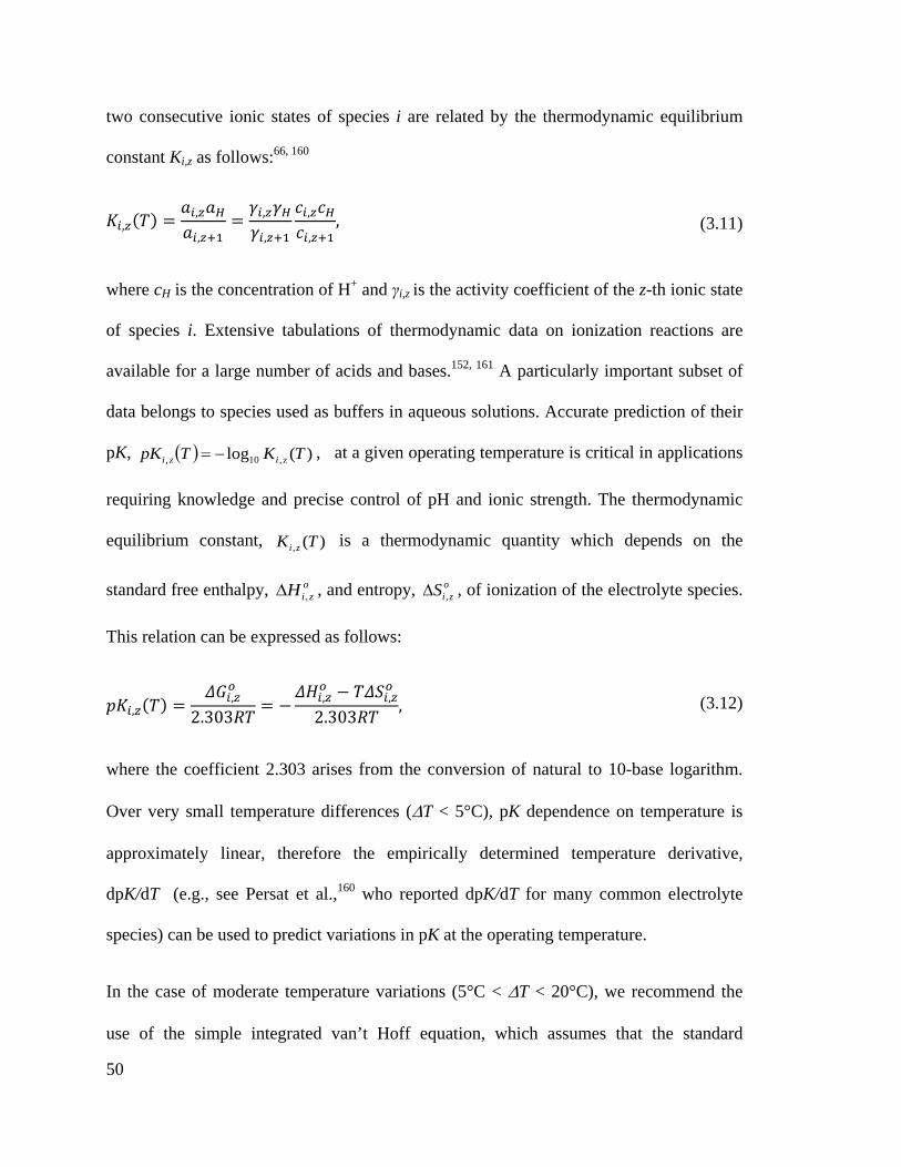
50

two consecutive ionic states of species i are related by the thermodynamic equilibrium

constant Ki,z as follows:66, 160

𝐾𝑖,𝑧(𝑇) =𝑎𝑖,𝑧𝑎𝐻𝑎𝑖,𝑧+1

=𝛾𝑖,𝑧𝛾𝐻𝛾𝑖,𝑧+1

𝑐𝑖,𝑧𝑐𝐻𝑐𝑖,𝑧+1

, (3.11)

where cH is the concentration of H+ and γi,z is the activity coefficient of the z-th ionic state

of species i. Extensive tabulations of thermodynamic data on ionization reactions are

available for a large number of acids and bases.152, 161 A particularly important subset of

data belongs to species used as buffers in aqueous solutions. Accurate prediction of their

pK, ( ) )(log ,10, TKTpK zizi −= , at a given operating temperature is critical in applications

requiring knowledge and precise control of pH and ionic strength. The thermodynamic

equilibrium constant, )(, TK zi is a thermodynamic quantity which depends on the

standard free enthalpy, oziH ,∆ , and entropy, o

ziS ,∆ , of ionization of the electrolyte species.

This relation can be expressed as follows:

𝑝𝐾𝑖,𝑧(𝑇) =𝛥𝐺𝑖,𝑧𝑜

2.303𝑅𝑇= −

𝛥𝐻𝑖,𝑧𝑜 − 𝑇𝛥𝑆𝑖,𝑧𝑜

2.303𝑅𝑇, (3.12)

where the coefficient 2.303 arises from the conversion of natural to 10-base logarithm.

Over very small temperature differences (∆T < 5°C), pK dependence on temperature is

approximately linear, therefore the empirically determined temperature derivative,

dpK/dT (e.g., see Persat et al.,160 who reported dpK/dT for many common electrolyte

species) can be used to predict variations in pK at the operating temperature.

In the case of moderate temperature variations (5°C < ∆T < 20°C), we recommend the

use of the simple integrated van’t Hoff equation, which assumes that the standard

51

enthalpy change, oziH ,∆ , and the standard entropy change, o

ziS ,∆ , are constant with

temperature. Differentiating Eq. (3.12) with respect to temperature, and then integrating

from θ to T gives

𝑝𝐾𝑖,𝑧(𝑇) = 𝑝𝐾𝑖,𝑧(𝜃) −𝛥𝐻𝑖,𝑧𝑜 (𝜃)2.303𝑅 �

1𝜃−

1𝑇�

. (3.13)

Eq. (3.13) can be used to evaluate zipK , at the operating temperature, T, provided that we

know the ( )θzipK , and ( )θoziH ,∆ . Goldberg et al.152 and Christensen et al.161 have an

extensive list for empirically determined thermodynamic properties (including zipK , and

oziH ,∆ ) of ions in aqueous solution (at K15.298=θ ). Our buffer simulation tool (see end

of Theory Section) includes a database of ( )θzipK , and ( )θoziH ,∆ for over 100 species.

Clarke and Glew relation (T<100°C):

Over wider temperature ranges, we recommend the Clarke and Glew approach,151

which accounts for the temperature dependence of the standard enthalpy, oziH ,∆ , and the

standard entropy change, oziS ,∆ , when deriving the representative function for )(, TpK zi ,

from Eq. (3.12). The temperature gradient of oziH ,∆ of species i, with valence z,

�𝜕∆𝐻𝑖,𝑧𝑜

𝜕𝑇�𝑝

= �∆𝐶𝑝𝑜�𝑖,𝑧, (3.14)

defines another thermodynamic quantity, the change in heat capacity at constant pressure,

ozipC ,,∆ .162 For many ionization reactions, the temperature dependence of o

ziS ,∆ also

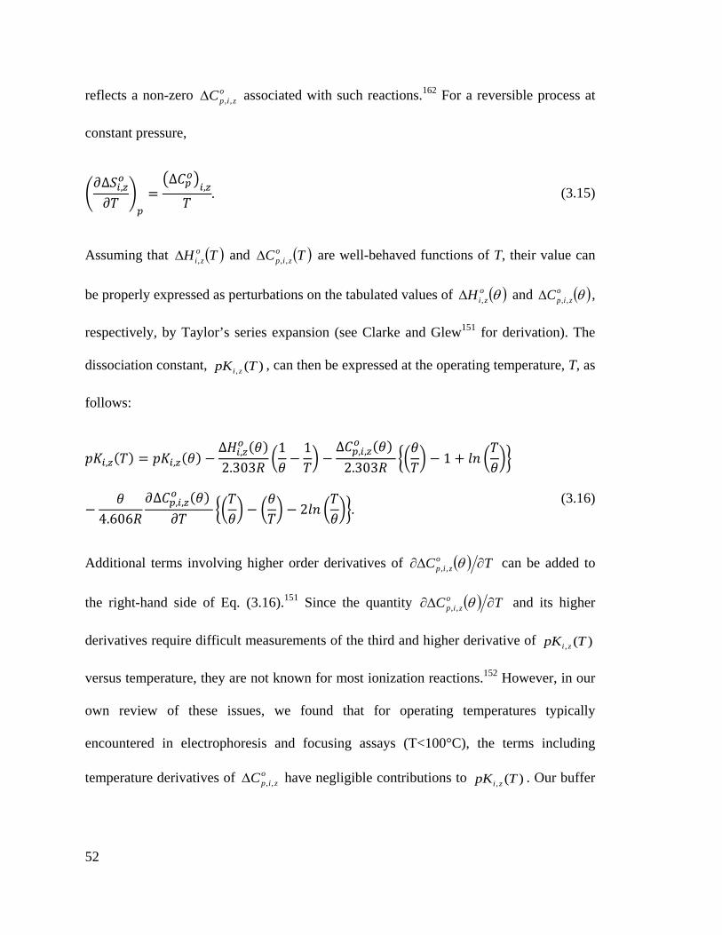
52

reflects a non-zero ozipC ,,∆ associated with such reactions.162 For a reversible process at

constant pressure,

�𝜕∆𝑆𝑖,𝑧𝑜

𝜕𝑇�𝑝

=�∆𝐶𝑝𝑜�𝑖,𝑧

𝑇. (3.15)

Assuming that ( )TH ozi,∆ and ( )TCo

zip ,,∆ are well-behaved functions of T, their value can

be properly expressed as perturbations on the tabulated values of ( )θoziH ,∆ and ( )θo

zipC ,,∆ ,

respectively, by Taylor’s series expansion (see Clarke and Glew151 for derivation). The

dissociation constant, )(, TpK zi , can then be expressed at the operating temperature, T, as

follows:

𝑝𝐾𝑖,𝑧(𝑇) = 𝑝𝐾𝑖,𝑧(𝜃) −∆𝐻𝑖,𝑧𝑜 (𝜃)2.303𝑅 �

1𝜃−

1𝑇�

−∆𝐶𝑝,𝑖,𝑧

𝑜 (𝜃) 2.303𝑅

��𝜃𝑇�

− 1 + 𝑙𝑛 �𝑇𝜃��

−𝜃

4.606𝑅𝜕∆𝐶𝑝,𝑖,𝑧

𝑜 (𝜃) 𝜕𝑇

��𝑇𝜃�

− �𝜃𝑇�

− 2𝑙𝑛 �𝑇𝜃��.

(3.16)

Additional terms involving higher order derivatives of ( ) TCozip ∂∆∂ θ,, can be added to

the right-hand side of Eq. (3.16).151 Since the quantity ( ) TCozip ∂∆∂ θ,, and its higher

derivatives require difficult measurements of the third and higher derivative of )(, TpK zi

versus temperature, they are not known for most ionization reactions.152 However, in our

own review of these issues, we found that for operating temperatures typically

encountered in electrophoresis and focusing assays (T<100°C), the terms including

temperature derivatives of ozipC ,,∆ have negligible contributions to )(, TpK zi . Our buffer

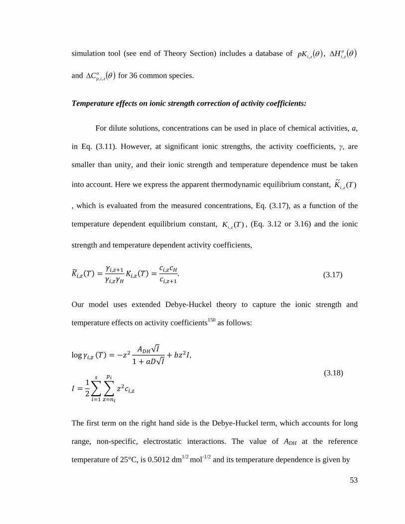
53

simulation tool (see end of Theory Section) includes a database of ( )θzipK , , ( )θoziH ,∆

and ( )θozipC ,,∆ for 36 common species.

Temperature effects on ionic strength correction of activity coefficients:

For dilute solutions, concentrations can be used in place of chemical activities, a,

in Eq. (3.11). However, at significant ionic strengths, the activity coefficients, γ, are

smaller than unity, and their ionic strength and temperature dependence must be taken

into account. Here we express the apparent thermodynamic equilibrium constant, )(~, TK zi

, which is evaluated from the measured concentrations, Eq. (3.17), as a function of the

temperature dependent equilibrium constant, )(, TK zi , (Eq. 3.12 or 3.16) and the ionic

strength and temperature dependent activity coefficients,

𝐾�𝑖,𝑧(𝑇) =𝛾𝑖,𝑧+1𝛾𝑖,𝑧𝛾𝐻

𝐾𝑖,𝑧(𝑇) =𝑐𝑖,𝑧𝑐𝐻𝑐𝑖,𝑧+1

. (3.17)

Our model uses extended Debye-Huckel theory to capture the ionic strength and

temperature effects on activity coefficients150 as follows:

log 𝛾𝑖,𝑧 (𝑇) = −𝑧2𝐴𝐷𝐻√𝐼

1 + 𝑎𝐷√𝐼+ 𝑏𝑧2𝐼,

𝐼 =12�� 𝑧2𝑐𝑖,𝑧

𝑝𝑖

𝑧=𝑛𝑖

𝑠

𝑖=1

(3.18)

The first term on the right hand side is the Debye-Huckel term, which accounts for long

range, non-specific, electrostatic interactions. The value of ADH at the reference

temperature of 25°C, is 0.5012 dm1/2 mol-1/2 and its temperature dependence is given by

54

𝐴𝐷𝐻 =𝑒3𝑁𝐴𝑣

1 2⁄

4𝜋√2(𝜀𝑘𝑇)3 2⁄ ln 10. (3.19)

As expected from the ( ) 231 Tε dependence, the variation of this parameter with

temperature is relatively small.150 Extended Debye-Huckel theory also takes into account

contributions from the finite nature of ions in the denominator (see discussion on term aD

in Section 2.3). The second term on the right hand side of Eq. (3.18) accounts for

specific, short-range, non-electrostatic interactions occurring at high ionic strengths, as

approximated by a linear, empirical correction term, b. The value of b at 25°C is 0.1 dm3

mol-1. b values at temperatures other than 25°C depend on the value adopted for aD.149

However, the variation of b with temperature, (db/dT)p, is less than 0.005 dm3 mol-1 K-

1.163, 164 The temperature effect of b is therefore very often negligible. For example, in the

range 0°C to 50°C, assuming a constant value of b, the error in Izi,logγ will be less

than 0.13 dm3 mol-1. This corresponds to a small uncertainty in zipK , of <0.026 at

I = 100 mM (see Eq. (3.17)). Therefore, in this study, we adopt constant values of

1.5 dm3/2 mol-1/2 for aD and 0.1 dm3 mol-1 for b for all temperatures.

To evaluate degree of ionization of species i, we use the apparent equilibrium

constant, )(~, TK zi , which accounts for both, temperature and ionic strength effects, in the

electroneutrality condition:67

�𝑐𝑖 � 𝑧𝑔𝑖,𝑧

𝑝𝑖

𝑧=𝑛𝑖

(𝑇)𝑠

𝑖=1

+ 𝑐𝐻 −𝐾�𝑤(𝑇)𝑐𝐻

= 0, (3.20)

55

where 𝑔𝑖,𝑧(𝑇) = 𝐿𝑖,𝑧(𝑇)𝑐𝐻𝑧 ∑ 𝐿𝑖,𝑧(𝑇)𝑐𝐻𝑧𝑝𝑖𝑧=𝑛𝑖� is the dissociation level of the species i, ci is

the total concentration, and ( ) ( ) )()(~ TTTKTK OHHWW γγ= is the apparent equilibrium

constant of water. Outside of the safe159 pH range (pH of 5 to 9), one must take into

account the variation in water equilibrium constant, ( )TKW , with temperature to

accurately determine the concentration of OH- and H+, and their contribution to

conductance. In the current model, we used the water properties ( )θWpK , ( )θoWH∆ and

( )θoWC∆ reported by Olofsson and Hepler.165 ( )TL zi, depends on the apparent equilibrium

constants as given by Bercovici et al.:67

𝐿𝑖,𝑧(𝑇) =

⎩⎪⎪⎨

⎪⎪⎧� 𝐾�𝑖,𝑧′(𝑇) 𝑧 < 0

−1

𝑧′= 𝑧1 𝑧 = 0

�𝐾�𝑖,𝑧′−1(𝑇) 𝑧 < 0.

𝑧−1

𝑧′= 0

(3.21)

3.2.5 Solution method for temperature model

Equations (3.5, 3.16, 3.17, 3.18, 3.20 and 3.21) therefore constitute our

temperature dependent model for effective mobility including the temperature effects on

viscosity, ion solvation, ionic strength correction and degree of ionization. To solve this

system, we first solve for the thermodynamic equilibrium constants of each species at the

operating temperature using Eq. (3.16), and then we propose an initial guess for 𝑐𝐻. We

take as an initial guess simply the solution of the Eq. (3.20) with zero ionic strength, and

use this to calculate the ionic concentrations, ci,z, activity coefficients, )(, Tziγ , and

apparent equilibrium constants, ( )TK zi,~ as per Eqs. (3.17, 3.18 and 3.21). Then, Eq.

56

(3.20) is solved repeatedly for ci,z by Newton iteration, until the solution for 𝑐𝐻 converges

to a value within a predefined tolerance. Similar solution methods were adopted by

Bercovici et al.67 and Bahga et al.66

The ionic strength obtained through this process is then used to calculate the fully ionized

actual mobility, )(, Tziµ , of every ionic species at the operating temperature, T, using our

version of extended (and modified) Onsager–Fuoss expression, Eq (3.5), which accounts

for viscosity, ion solvation, and ionic strength effects with temperature. This actual

mobility of species i is then corrected to the effective mobility, as given by

𝜇𝑖(𝑇) = � 𝜇𝑖,𝑧(𝑇)𝑝𝑖

𝑧=𝑛𝑖

𝑔𝑖,𝑧(𝑇), (3.22)

using the temperature dependent dissociation factor, )(, Tg zi .67

3.2.6 Quantifying the aggregate effect of temperature dependences unrelated to viscosity

In this study, we address all major physical phenomena associated with the

temperature dependence of electrolyte mobility in water. The easiest, most common, and

often most pronounced effect to take into account is the temperature dependence of

viscosity of water. We introduce factor f, which normalizes the electrolyte solution

conductance by the change associated with variations in viscosity as follows:

( ) ( )( ) ( )TT

fησθηθσ

= (3.23)

Here, conductivity, σ, is defined as

57

𝜎(𝑇) = �𝑐𝑖 � 𝐹𝑧𝑖𝜇𝑖,𝑧(𝑇)𝑝𝑖

𝑧=𝑛𝑖

𝑔𝑖,𝑧(𝑇)𝑠

𝑖=1

. (3.24)

f therefore quantifies the aggregate effect of all phenomena other than simple changes in

solvent viscosity. Namely, f describes the net effect on conductivity due to temperature-

dependent changes in degree of ionization, ion solvation, and ionic strength corrections.

An ideal ion which follows Walden’s rule exactly has an f value of unity )0(log10 =f .

The sign of f10log indicates if these effects act in concert with or against the influence

of viscosity on electrolyte solution conductivity (these effects oppose the influence of

viscosity on buffer conductivity with positive f10log ). This useful parameter and its

application were first proposed by Ross and Locascio131 in 2002 and is relevant for many

electrophoresis effects including joule heating, dispersion, and voltage versus current

requirements.

3.2.7 Stand-alone simulation tool for temperature-dependent electrolyte properties

We developed a MATLAB (R2012b Mathworks, Natick, MA) based simulation

tool for electrolyte solutions which incorporates our comprehensive temperature model.

This simulation tool inputs mobilities and thermophysical data and calculates system pH,

system conductivity, and effective mobilities for arbitrary mixtures of strong or weak

electrolytes. The electrophoretic mobilities of all analytes presented in this study (except

water ions) were obtained from Hirokawa et al.166 The ionization dissociation constants,

)(, θzipK , standard molar enthalpy change, )(, θoziH∆ , and standard molar heat capacity

change, )(,, θozipC∆ , of each species were obtained from Goldberg at al.152 (see Table 3.2).

58

We also offer an extended list of analytes with their chemical properties built into a

graphical user interface of the Matlab script. When available, we list all four of the

chemical properties. However, for the some ionic species, data on )(,, θozipC∆ is not

available, in which case, we list only the mobility, )(, θµ zi ,166 )(, θzipK ,161 and )(, θoziH∆

.161 Our code, which we named Simulation of Temperature Effects on ElectroPhoresis

(STEEP), is available for free on our website at

http://microfluidics.stanford.edu/download/index.html. We include source code, a data

base of thermophysical data, and instructions for use.

59

Tab

le 3

.2. L

ist o

f che

mic

al sp

ecie

s mob

ility

, μ, (

in 1

09 m

2 V-1

s-1) ,

pK

, sta

ndar

d fr

ee e

ntha

lpy

of io

niza

tion,

∆Ho , (

in J

mol

-1)

stan

dard

fr

ee sp

ecifi

c he

at o

f ion

izat

ion,

∆Cpo ,

(in J

K-1

mol

-1) v

alue

s def

ined

at 2

5°C

, as u

sed

in m

ain

pape

r.

Nam

eμ(-3)μ(-2)μ(-1)μ(+1)p

K(-3

)pK

(-2)p

K(-1

)pK

(+1)ΔH

°(-3)Δ

H°(-2)ΔH

°(-1)ΔH

°(+1) Δ

Cp°

(-3)ΔC

p°(-2

)ΔC

p°(-1

)ΔC

p°(+

1)A

CET

IC A

CID

42.4

4.75

6-4

10-1

42BO

RIC

AC

ID36

.59.

237

1380

0-2

40C

ITRI

C A

CID

74.4

54.7

28.7

6.39

64.

761

3.12

8-3

380

2230

4070

-254

-178

-131

HEP

ES23

.57.

564

2040

047

HY

DRO

CH

LORI

C A

CID

79.1

-20

0M

OPS

26.9

7.18

421

100

25PH

OSP

HO

RIC

AC

ID71

.561

.434

.612

.35

7.19

82.

148

1600

036

00-8

000

-242

-230

-141

BIST

RIS

266.

484

2840

027

ETH

AN

OLA

MIN

E44

.39.

498

5052

026

HIS

TID

INE

28.3

28.8

9.34

6.07

4380

029

500

-233

176

POTA

SSIU

M76

.213

00

SOD

IUM

51.9

13.7

00

TRIS

29.5

8.07

247

450

-59

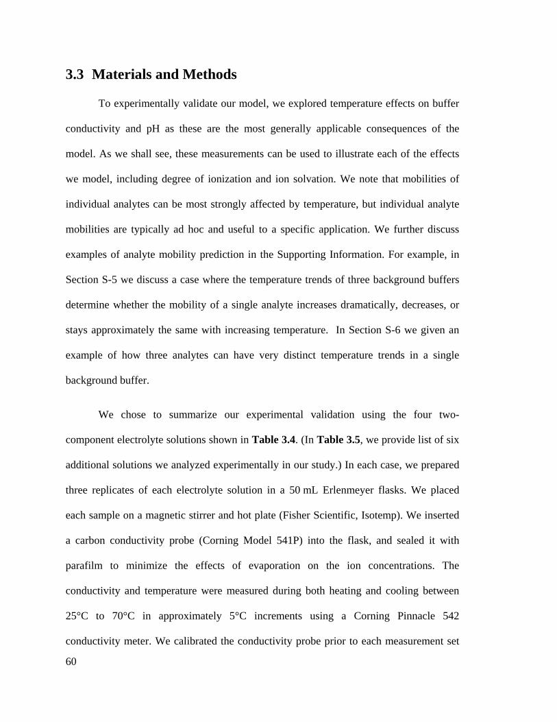
60

3.3 Materials and Methods

To experimentally validate our model, we explored temperature effects on buffer

conductivity and pH as these are the most generally applicable consequences of the

model. As we shall see, these measurements can be used to illustrate each of the effects

we model, including degree of ionization and ion solvation. We note that mobilities of

individual analytes can be most strongly affected by temperature, but individual analyte

mobilities are typically ad hoc and useful to a specific application. We further discuss

examples of analyte mobility prediction in the Supporting Information. For example, in

Section S-5 we discuss a case where the temperature trends of three background buffers

determine whether the mobility of a single analyte increases dramatically, decreases, or

stays approximately the same with increasing temperature. In Section S-6 we given an

example of how three analytes can have very distinct temperature trends in a single

background buffer.

We chose to summarize our experimental validation using the four two-

component electrolyte solutions shown in Table 3.4. (In Table 3.5, we provide list of six

additional solutions we analyzed experimentally in our study.) In each case, we prepared

three replicates of each electrolyte solution in a 50 mL Erlenmeyer flasks. We placed

each sample on a magnetic stirrer and hot plate (Fisher Scientific, Isotemp). We inserted

a carbon conductivity probe (Corning Model 541P) into the flask, and sealed it with

parafilm to minimize the effects of evaporation on the ion concentrations. The

conductivity and temperature were measured during both heating and cooling between

25°C to 70°C in approximately 5°C increments using a Corning Pinnacle 542

conductivity meter. We calibrated the conductivity probe prior to each measurement set

61

using conductivity standards purchased from Ricca Chemical Company. Using the

system’s Pinnacle “3 in 1” Premium Gel Combo electrode, we also measured the pH of

each electrolyte solution at 25°C and 70°C. Data obtained during either heating or

cooling track each other closely, consistent with negligible hysteresis effects in our

method.

3.4 Results and discussion

3.4.1 Predictions of effective mobility, conductivity, and pH

To demonstrate our model, we selected three example buffers which demonstrate

the phenomena discussed in Theory. Figures 1-3 show plots of the effective mobility of

the titrating anion for temperatures from 20°C to 80°C, with respect to its effective

mobility at the reference temperature, C°= 25θ , as follows: )_()_( θµµ T (the

subscript indicates an anion). The curves associated with our full temperature model

(including all effects considered here) are labeled “Current”. In the upper insets of

Figures 1-3, we show predictions of the full temperature model for the anion and cation

pKs and electrolyte solution pH as functions of temperature. In the lower insets, we show

plots of ionic strength, I, and normalized electrolyte solution conductance, f, as functions

of temperature.

The main plots of Figure 3.1-3.3 also include four additional curves which we

use to demonstrate the effect of individual physical phenomena described in Theory.

These curves represent incomplete versions of our model, and are described in Table 3.3.

All curves correct for changes in water viscosity. The simplest model, ‘W’, uses only the

Walden’s viscosity correction term, α, to evaluate effective mobility at elevated

62

temperature. Model ‘SSC’ captures the temperature dependence of limiting ionic

mobility due to changes in solvation, but disregards changes in degree of ionization and

the temperature sensitivity of ionic strength corrections. Model ‘ISC’ quantifies the

temperature dependence of the extended Onsager-Fuoss and the extended Debye-Huckel

theory, but the degree of ionization and the ion solvation correction terms are to always

equal the value at room temperature. Model ‘pKC’, captures the temperature effects on

degree of ionization, but assumes that ion solvation and the ionic strength correction

terms are always equal to the value at room temperature.

Table 3.3 Summary of full model (labeled “Current” in Figures 1-3) and limiting models used for

comparing the various sources of temperature effects on effective ionic mobility. The values )(, θµ zi and

)(, Tziµ are evaluated using Eq (3.22). )(, θzig , and )(, Tg zi are evaluated using Eq (3.20). The

assumptions made for the limiting models include temperature insensitivity of ion solvation, )1( =iβ ,

temperature-independent degree of ionization ( 0/ =dTdpK ), and temperature independent ionic

strength corrections ))"(.(" TfcorrIS ≠ . T is the operating temperature and θ is the reference

temperature (25°C).

Effective mobility at operating temperature, T Assumptions

Current 𝜇𝑖(𝑇) = � 𝜇𝑖,𝑧(𝑇)𝑝𝑖

𝑧=𝑛𝑖

𝑔𝑖,𝑧(𝑇)

W 𝜇𝑖(𝑇) = 𝛼 � 𝜇𝑖,𝑧(𝜃)𝑝𝑖

𝑧=𝑛𝑖

𝑔𝑖,𝑧(𝜃)

𝛽𝑖 = 1

𝑑𝑝𝐾 𝑑𝑇 = 0⁄ 𝐼𝑆 𝑐𝑜𝑟𝑟.≠ 𝑓(𝑇)

SSC 𝜇𝑖(𝑇) = 𝛼𝛽𝑖 � 𝜇𝑖,𝑧(𝜃)𝑝𝑖

𝑧=𝑛𝑖

𝑔𝑖,𝑧(𝜃)

𝑑𝑝𝐾 𝑑𝑇 = 0⁄ 𝐼𝑆 𝑐𝑜𝑟𝑟.≠ 𝑓(𝑇)

ISC 𝜇𝑖(𝑇) = � 𝜇𝑖,𝑧(𝑇)𝑝𝑖

𝑧=𝑛𝑖

𝑔𝑖,𝑧(𝑇)

𝛽𝑖 = 1 𝑑𝑝𝐾 𝑑𝑇 = 0⁄

pKC 𝜇𝑖(𝑇) =∑ 𝜇𝑖,𝑧(𝜃)𝑝𝑖𝑧=𝑛𝑖 𝑔𝑖,𝑧(𝜃)

�∑ 𝜇𝑖,𝑧(𝜃)𝑝𝑖𝑧=𝑛𝑖 𝑔𝑖,𝑧(𝜃)�

(𝐼=0)

� �𝜇𝑖,𝑧(𝑇)𝑔𝑖,𝑧(𝑇)�(𝐼=0)

𝑝𝑖

𝑧=𝑛𝑖

𝛽𝑖 = 1 𝐼𝑆 𝑐𝑜𝑟𝑟.≠ 𝑓(𝑇)

63

Figure 3.1 shows predictions for a simple, two-component buffer consisting of a

univalent weak electrolyte, 200 mM Tris, and a univalent, strong titrant anion donated by

100 mM HCl (pH = 8.18 at C°= 25θ ). The main plot shows Cl- mobility normalized by

its value at the reference temperature, θ. The anion mobility increases monotonically

from 20°C to 80°C. We see that the comparison curves W, ISC, and pKC each

overpredict anion mobility by about the same amount, while the SSC model matches the

prediction quite closely. Here, the water viscosity has the most prominent influence on

the effective mobility of the chloride ion. The most dominant, non-viscous related effect

is due to changes in the solvation of Cl-. The Stokes radius of Cl- increases with

temperature resulting in reduction of its absolute electrophoretic mobility. The top inset

plot shows that the buffer pH tracks closely the pK of the buffering Tris, as expected,

since the titrant ion Cl- is donated by a strong acid so the ionization of Tris is independent

of pH. For the same reason, the ionic strength of the solution (lower inset) is constant

(since dissociation of Tris is determined by the concentration of the pH-insensitive Cl-).

The slight overprediction by the SSC model is associated with a mild temperature

sensitivity of the Onsager-Fuoss correction. Overall, we note that simple buffers

consisting of a weak electrolyte titrated with a strongly ionized (titrant) ion typically have

uniform ionic strength but have a pH change with temperature dictated by the pK(T)

function of the weak electrolyte.

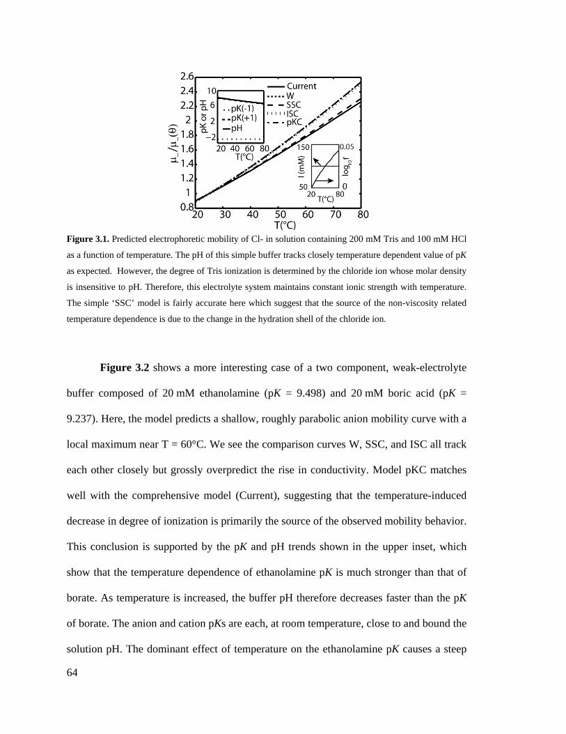
64

Figure 3.1. Predicted electrophoretic mobility of Cl- in solution containing 200 mM Tris and 100 mM HCl

as a function of temperature. The pH of this simple buffer tracks closely temperature dependent value of pK

as expected. However, the degree of Tris ionization is determined by the chloride ion whose molar density

is insensitive to pH. Therefore, this electrolyte system maintains constant ionic strength with temperature.

The simple ‘SSC’ model is fairly accurate here which suggest that the source of the non-viscosity related

temperature dependence is due to the change in the hydration shell of the chloride ion.

Figure 3.2 shows a more interesting case of a two component, weak-electrolyte

buffer composed of 20 mM ethanolamine (pK = 9.498) and 20 mM boric acid (pK =

9.237). Here, the model predicts a shallow, roughly parabolic anion mobility curve with a

local maximum near T = 60°C. We see the comparison curves W, SSC, and ISC all track

each other closely but grossly overpredict the rise in conductivity. Model pKC matches

well with the comprehensive model (Current), suggesting that the temperature-induced

decrease in degree of ionization is primarily the source of the observed mobility behavior.

This conclusion is supported by the pK and pH trends shown in the upper inset, which

show that the temperature dependence of ethanolamine pK is much stronger than that of

borate. As temperature is increased, the buffer pH therefore decreases faster than the pK

of borate. The anion and cation pKs are each, at room temperature, close to and bound the

solution pH. The dominant effect of temperature on the ethanolamine pK causes a steep

65

drop in pH. This decreases the ionization of borate ion, thereby decreasing its effective

mobility. The associated drop in the ionic strength (bottom inset), I, also influences the

effective mobility by decreasing the magnitude of the Onsager-Fuoss correction (which

explains the slight underprediction of pKC model from Current). Again, the large,

positive value for log10f (up to log10f = 0.33 or f = 2.2 at T = 80°C) shows how these

effects act together to strongly compensate for the decrease in water viscosity. These

predictions show a discrepancy between the full model and of the Walden model by as

much as 116% for the anion mobility.

Figure 3.2. Predicted electrophoretic mobility versus temperature of boric acid anion (borate) in solution

containing 20 mM ethanolamine and 20 mM boric acid. Increase in temperature results in strong drop in pK

of ethanolamine and a moderate drop in the pK of boric acid, resulting in an overall decrease in pH (top

inset). Here, the most prominent contribution to both anion mobility and ionic strength, I (bottom inset) is

due to the sharp decrease in degree of ionization of boric acid (hence the proximity of ‘pKC’ model to

‘Current’). The large, positive value of log10 𝑓 (bottom inset) shows how this effect opposes contributions

from the decreasing viscosity to conductivity. Ultimately, these opposing effects are also reflected by the

shallow mobility curve (main plot). Predictions based on Walden’s rule here overestimate the anion

mobility by 116% (and buffer conductivity by 106%).

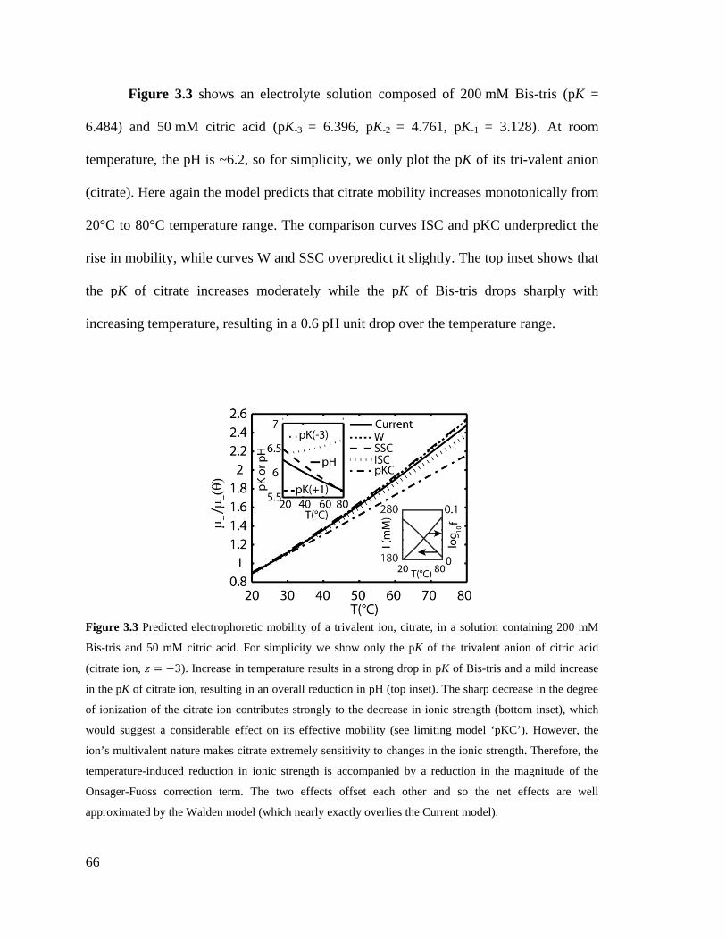
66

Figure 3.3 shows an electrolyte solution composed of 200 mM Bis-tris (pK =

6.484) and 50 mM citric acid (pK-3 = 6.396, pK-2 = 4.761, pK-1 = 3.128). At room

temperature, the pH is ~6.2, so for simplicity, we only plot the pK of its tri-valent anion

(citrate). Here again the model predicts that citrate mobility increases monotonically from

20°C to 80°C temperature range. The comparison curves ISC and pKC underpredict the

rise in mobility, while curves W and SSC overpredict it slightly. The top inset shows that

the pK of citrate increases moderately while the pK of Bis-tris drops sharply with

increasing temperature, resulting in a 0.6 pH unit drop over the temperature range.

Figure 3.3 Predicted electrophoretic mobility of a trivalent ion, citrate, in a solution containing 200 mM

Bis-tris and 50 mM citric acid. For simplicity we show only the pK of the trivalent anion of citric acid

(citrate ion, 𝑧 = −3). Increase in temperature results in a strong drop in pK of Bis-tris and a mild increase

in the pK of citrate ion, resulting in an overall reduction in pH (top inset). The sharp decrease in the degree

of ionization of the citrate ion contributes strongly to the decrease in ionic strength (bottom inset), which

would suggest a considerable effect on its effective mobility (see limiting model ‘pKC’). However, the

ion’s multivalent nature makes citrate extremely sensitivity to changes in the ionic strength. Therefore, the

temperature-induced reduction in ionic strength is accompanied by a reduction in the magnitude of the

Onsager-Fuoss correction term. The two effects offset each other and so the net effects are well

approximated by the Walden model (which nearly exactly overlies the Current model).

67

The decrease in pH results in an overall strong decrease in ionic strength by promoting

reassociation of the citrate ion with hydrogen. However, the effective mobility of the

trivalent citrate is only mildly reduced, because a decrease in ionic strength also strongly

attenuates ionic strength effects on mobility. Interestingly, in this system including a

multivalent electrolyte, the two effects (pK(T) affecting dissociation and ionic strength on

mobility) largely offset each other.

3.4.2 Additional electrolyte examples

Here we include additional curves which we use to demonstrate the effect of

individual physical phenomena described in the Table 3.4. For clarity, if one of the

physical phenomena has no temperature contribution to mobility (other than a Walden

type behavior), and its corresponding limiting model overlaps with model ‘W’; we chose

not to plot the curve. Figure 3.4 shows predictions for the second electrolyte in Table 3,

which is composed of 50 mM potassium citrate (pK-3 = 6.396, pK-2 = 4.761, pK-1 = 3.128)

mixed with 200 mM Bis-tris (pK = 6.484). Citric acid is trivalent and is therefore very

sensitive to ionic strength effects. Further, potassium is a small ion whose hydration

changes with temperature. We also added weak Bis-tris to increase the pH. We chose this

solution as a large difference between the pH and citrate pKs ensures that citrate remains

fully ionized for all temperatures. This enables the isolation of two temperature related

phenomena: ionic strength effects on citrate ion mobility (right plot) and ion solvation

effect on the potassium ion mobility (left plot). Note that, since pH > pKBis-tris - 2, Bis-tris

is practically neutral and has virtually zero effective mobility. Bis-tris therefore has

negligible contribution to solution ionic strength and conductivity. This solution is an

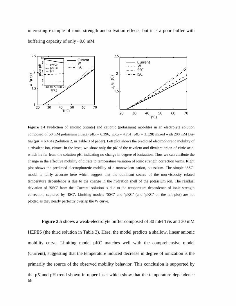
68

interesting example of ionic strength and solvation effects, but it is a poor buffer with

buffering capacity of only ~0.6 mM.

Figure 3.4 Prediction of anionic (citrate) and cationic (potassium) mobilites in an electrolyte solution

composed of 50 mM potassium citrate (pK-3 = 6.396, pK-2 = 4.761, pK-1 = 3.128) mixed with 200 mM Bis-

tris (pK = 6.484) (Solution 2, in Table 3 of paper). Left plot shows the predicted electrophoretic mobility of

a trivalent ion, citrate. In the inset, we show only the pK of the trivalent and divalent anion of citric acid,

which lie far from the solution pH, indicating no change in degree of ionization. Thus we can attribute the

change in the effective mobility of citrate to temperature variation of ionic strength correction terms. Right

plot shows the predicted electrophoretic mobility of a monovalent cation, potassium. The simple ‘SSC’

model is fairly accurate here which suggest that the dominant source of the non-viscosity related

temperature dependence is due to the change in the hydration shell of the potassium ion. The residual

deviation of ‘SSC’ from the ‘Current’ solution is due to the temperature dependence of ionic strength

correction, captured by ‘ISC’. Limiting models ‘SSC’ and ‘pKC’ (and ‘pKC’ on the left plot) are not

plotted as they nearly perfectly overlap the W curve.

Figure 3.5 shows a weak-electrolyte buffer composed of 30 mM Tris and 30 mM

HEPES (the third solution in Table 3). Here, the model predicts a shallow, linear anionic

mobility curve. Limiting model pKC matches well with the comprehensive model

(Current), suggesting that the temperature induced decrease in degree of ionization is the

primarily the source of the observed mobility behavior. This conclusion is supported by

the pK and pH trend shown in upper inset which show that the temperature dependence

69

of Tris pK is much stronger than that of HEPES. At room temperature, the anion and

cation pKs are close to and bound the solution pH. As temperature is increased, the buffer

pH decreases faster than the pK of HEPES. This decreases the ionization of HEPES ion,

thereby decreasing its effective mobility.

Figure 3.5 Predicted electrophoretic mobility versus temperature for HEPES (anion) in the solution of 30

mM Tris and 30 mM HEPES (Solution 3, in Table 3 of main paper). Increase in temperature results in a

strong drop in the pK of Tris and a moderate drop in the pK of HEPES, resulting in an overall decrease in

pH (inset). Here, the most prominent contribution to anion mobility is due to the sharp reduction in degree

of ionization of HEPES (hence the proximity of ‘pKC’ model to ‘Current’). Predictions based on Walden

rule here overestimate the anion mobility by 30% at 70°C. Limiting models ‘SSC’ and ‘ISC’ are not

plotted as they nearly perfectly overlap the W curve.

Figure 3.6 shows a weak-electrolyte buffer composed of 30 mM Tris and 15 mM

acetic acid (Solution 4 in Table 3.4). Here, the comprehensive model (Current) tracks

model ‘W’ closely, suggesting temperature effects on ion solvation, ionic strength

correction, and degree of ionization are insignificant. The latter conclusion is supported

by the pK and pH trend shown in upper inset of Figure 3.6. Tris is included at twice the

concentration of acetic acid, so the solution pH is dominated the pK(T) function of Tris.

The large difference (>2 units for all temperatures) between the acetate pK and solution

70

pH ensures the acetate remains fully ionized for all temperatures. In this electrolyte

solution, the mobility of acetate can be estimated by correcting for changes in viscosity of

water alone.

Figure 3.6 Predicted electrophoretic mobility versus temperature of acetate (anion) in a solution containing

30 mM Tris and 15 mM acetic acid (Solution 4, in Table 3.3). Here, ionic strength of solution containing

cation (Tris) and titrant (acetic acid) are determined by the molarity of the fully-ionized acetic acid. While

the pH varies with temperature dictated by the pK(T) function of the Tris, the large difference (>2 units for

all T) between acetate pK and solution pH ensures that acetic acid remains fully ionized. Therefore, the

acetate mobility predictions based on Walden’s rule estimate anion mobility fairly accurately, within ~4%.

Limiting models ‘SSC’, ‘ISC’, and ‘pKC’ are not plotted as they nearly perfectly overlap the W curve.

3.4.3 Temperature model validation

We validated our model using conductivity and pH measurements in the

temperature range of 25°C to 70°C for the two-component electrolyte solutions listed in

Table 3.4. For convenience of presentation, we present the data in terms of the f factor,

which quantifies temperature dependence that is not attributed to variations in water

viscosity (see Theory). Presentation of the experimental data in terms of f therefore also

offers a direct comparison with the commonly applied Walden’s rule. We also plot the

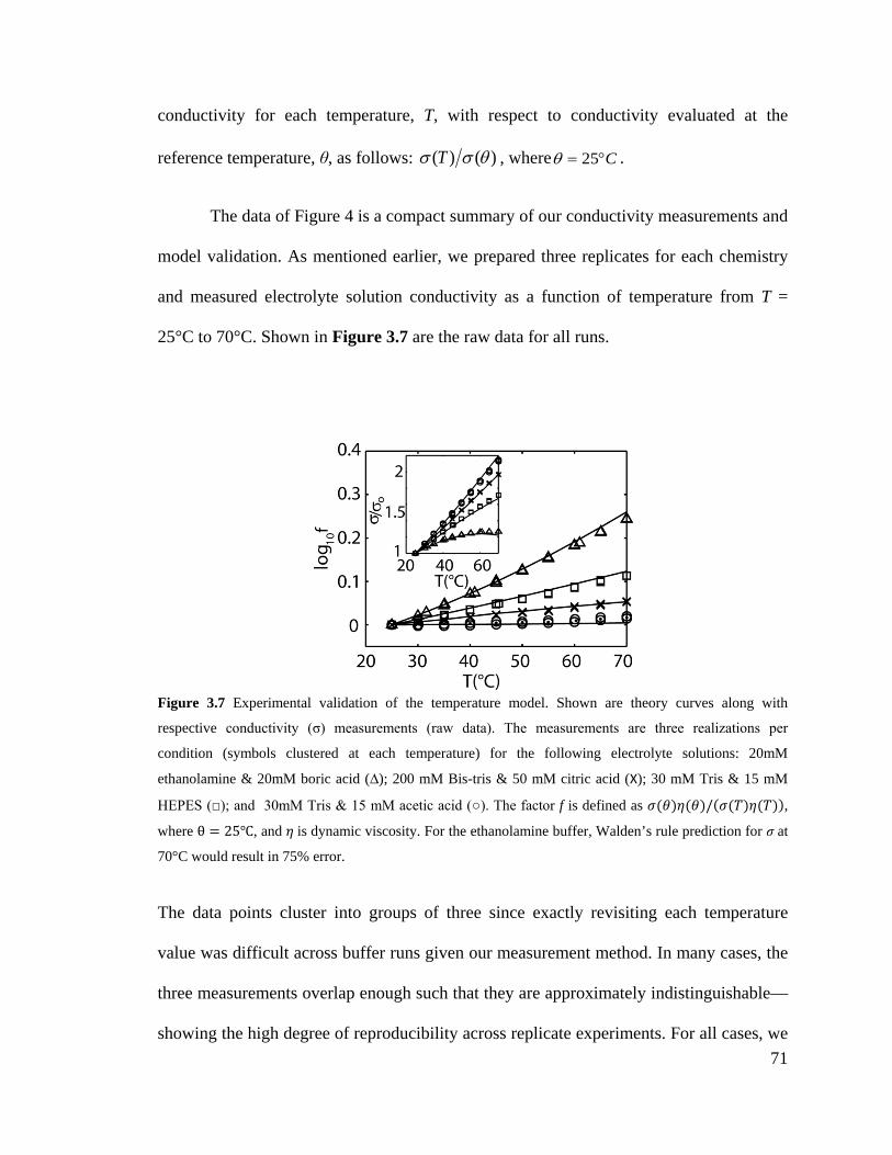
71

conductivity for each temperature, T, with respect to conductivity evaluated at the

reference temperature, θ, as follows: )()( θσσ T , where C°= 25θ .

The data of Figure 4 is a compact summary of our conductivity measurements and

model validation. As mentioned earlier, we prepared three replicates for each chemistry

and measured electrolyte solution conductivity as a function of temperature from T =

25°C to 70°C. Shown in Figure 3.7 are the raw data for all runs.

Figure 3.7 Experimental validation of the temperature model. Shown are theory curves along with

respective conductivity (σ) measurements (raw data). The measurements are three realizations per

condition (symbols clustered at each temperature) for the following electrolyte solutions: 20mM

ethanolamine & 20mM boric acid (∆); 200 mM Bis-tris & 50 mM citric acid (X); 30 mM Tris & 15 mM

HEPES (□); and 30mM Tris & 15 mM acetic acid (○). The factor f is defined as 𝜎(𝜃)𝜂(𝜃)/(𝜎(𝑇)𝜂(𝑇)),

where θ = 25℃, and 𝜂 is dynamic viscosity. For the ethanolamine buffer, Walden’s rule prediction for σ at

70°C would result in 75% error.

The data points cluster into groups of three since exactly revisiting each temperature

value was difficult across buffer runs given our measurement method. In many cases, the

three measurements overlap enough such that they are approximately indistinguishable—

showing the high degree of reproducibility across replicate experiments. For all cases, we

72

also decreased temperature from T = 70°C down to T = 25°C and measured conductivity

at 5°C increments (not shown here) to ensure our experiment showed no hysteresis

effects (e.g., due to unwanted evaporation of water during the run). None of the data

demonstrated a dependence on the sign of temperature increase. Shown together with the

raw data are predictions from the ‘Current’, full temperature model (solid curve).

In Fig. 4, the solution of ethanolamine and boric acid (parabola) shows

conductivity which is concave down and parabolic similar to the predicted anion mobility

curve shown in Fig. 2. The conductivity increases by a maximum of only 25%, due to the

steep decline of ionization of both borate and ethanolamine ions (c.f Figure 3.2 for more

details). The solutions Bis-tris-potassium citrate and Tris-hepes also show increases in

conductivity, but with shallower slopes, and associated higher values of log10f. The Bis-

tris and potassium citrate conductivity changes are influenced mostly by the change in

solvation of the potassium ion and by the temperature dependence of the ionic strength

corrections (citrate is trivalent and therefore its mobility is very sensitive to ionic

strength, see Fig. S-1). The conductivity dependence of Tris-hepes is dominated by the

change in degree of ionization of its constituent weak electrolyte ions (see Figure 3.5 for

more details). The conductivity increases by 70% for Tris-hepes and by 100% for Bis-tris

and potassium citrate (from T = 25°C to T = 70°C). The electrolyte mixture of Tris and

acetic acid has the strongest temperature dependence. We see that this buffer also shows

the smallest and nearly constant values of log10f, suggesting that this buffer’s temperature

dependence is mostly due to the Walden type dependence (Figure 3.6). In all four

electrolyte solutions, the highlighted effects oppose the influence of viscosity (Walden)

on conductivity (positive log10f). At T = 70°C, Walden’s rule would yield the following

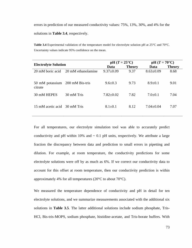
73

errors in prediction of our measured conductivity values: 75%, 13%, 30%, and 4% for the

solutions in Table 3.4, respectively.

Table 3.4 Experimental validation of the temperature model for electrolyte solution pH at 25°C and 70°C.

Uncertainty values indicate 95% confidence on the mean.

Electrolyte Solution pH (T = 25°C) pH (T = 70°C) Data Theory Data Theory

20 mM boric acid 20 mM ethanolamine 9.37±0.09 9.37 8.63±0.09 8.68

50 mM potassium citrate

200 mM Bis-tris 9.6±0.3 9.73 8.9±0.1 9.01

30 mM HEPES 30 mM Tris 7.82±0.02 7.82 7.0±0.1 7.04

15 mM acetic acid 30 mM Tris 8.1±0.1 8.12 7.04±0.04 7.07

For all temperatures, our electrolyte simulation tool was able to accurately predict

conductivity and pH within 10% and ~ 0.1 pH units, respectively. We attribute a large

fraction the discrepancy between data and prediction to small errors in pipetting and

dilution. For example, at room temperature, the conductivity predictions for some

electrolyte solutions were off by as much as 6%. If we correct our conductivity data to

account for this offset at room temperature, then our conductivity prediction is within

approximately 4% for all temperatures (20°C to about 70°C).

We measured the temperature dependence of conductivity and pH in detail for ten

electrolyte solutions, and we summarize measurements associated with the additional six

solutions in Table 3.5. The latter additional solutions include sodium phosphate, Tris-

HCl, Bis-tris-MOPS, sodium phosphate, histidine-acetate, and Tris-borate buffers. With

74

the sole exception of Tris-borate buffers, the conductivity and pH predictions agreed to

measured values within 4% and 0.2 pH units or better. These data suggest the model can

accurately predict the temperature dependence of electrolyte solution conductivity for all

the electrolyte solution explored, again with the exception of Tris-boric acid.

Interestingly we are able to well predict the behavior of Tris and of boric acid when these

species are paired with other ions we explored. However, the particular combination of

Tris and boric acid consistently showed large discrepancies between model and

measurements of conductivity and pH (respectively, 17 to 68% and as much as 0.32 pH

units). We hypothesize that Tris and boric acid ions may undergo non-acid/base reactions

with each other (see Supplementary Information). This hypothesis is strongly supported

by the work of Michov,167 which showed that Tris-borate buffers contain a cyclic

complex compound of betainic structure, and a buffer with both of these ions therefore

does not obey the Henderson-Hasselbalch equation.

Table 3.5 Summary of predictions and measurements of pH and conductivity for six additional electrolyte

solutions at temperatures 25°C and 70°C.

Composition pH (T=25°C) pH (T=70°C)

pHexp pHth σexp (μS/cm)

σth (μS/cm) pHexp pHth σexp

(μS/cm) σth

(μS/cm) 30 mM Bis-tris

30 mM MOPS 6.75 6.83 466 444 6.19 6.25 945 868

30 mM NaOH

20 mM phosphoric acid

7.22 6.98 2620 2463 7.21 6.99 5780 5358

20 mM L-histidine

20 mM acetic acid 5.34 5.41 1017 1013 5.03 5.07 1795 1796

200 mM Tris

100 mM HCL 8.19 8.15 4470 4527 7.12 7.10 8970 9378

10 mM Tris

10 mM boric acid 8.55 8.65 115 131 7.82 8.00 142 118

100 mM Tris

100 mM boric acid 8.31 8.65 749 1258 7.68 8.00 1414 1161

75

76

4 Particle Tracking and Multispectral Collocation Method for Cytometry-Like and Particle-to-Particle Binding Assays

The contents of this chapter are under review in Analytical Chemistry. They are

reproduced here with minor modifications.

4.1 Introduction

Accompanying the growing number of particle, cell, and bead-based assay

applications,86, 168-172 particle and cell analysis methods have become more rigorous and

sophisticated.173, 174 The two most frequently cited techniques are likely flow-cytometry

(FCM)174, 175 and laser-scanning cytometry (LSC).176 Flow cytometry is a workhorse

technology used routinely in immunology,177 pathology178 and hemotology.179 FCM

performs a single high content multiparametric measurement for thousands of particles in

minutes or less. (Here we shall use “particles” to denote micron-scale beads and/or living

cells.) The core of a standard cytometer is a flow chamber where a particle-laden stream

is hydrodynamically focused with the aid of sheath flow into a small interrogation region

through which particles traverse one at a time. Multicolor lasers illuminate particles in the

interrogation region. Forward scatter is approximately correlated to the size of the

particle and side scatter provides an indication of particle granularity.175 Increasing need

for multiplexing via polychromatic excitation and emission has pushed the frontiers of

flow cytometry, and enabled, for example, implementation of instruments that measure

up to 19 parameters (17 fluorescent colors and 2 physical parameters).177

77

Laser-Scanning Cytometry (LSC)176 was originally designed to provide an

imaging complement to traditional FCM and allow morphological analysis of adherent

cells.180 LSC scans stationary particles (typically cells) adhered to a surface and its

implementation has evolved to include analyses of cell proliferation, tissue architecture,

and immunophenotyping using precious samples.169 The cells are fixed onto slides and

scanned with multiple lasers. This can be repeated over time for studies of enzyme

kinetics and other time-resolved processes. The slide can be removed from the instrument

in order to change staining or otherwise modify the cells; and it can then be placed back

on the instrument for re-analysis.180 Each cell can be relocated and all of the data points

can be correlated for multivariate analysis.

There is a range of other multicolor particle image counting and analysis systems.

For example, recently the field has seen development of imaging versions of FCM

systems wherein point detectors are replaced by high speed imaging to analyze particle

morphology in more detail and using up to 12 wavelengths (e.g., the Amnis Imagestream

system). These systems employ time delay integration (TDI) wherein the camera is

panned electronically to track the cells in the flow stream. These systems track cell

velocities and use this to time the shift of photoelectrons on the CCD chip. These

systems can produce up to 12 simultaneous realizations of a darkfield, two brightfield

images, and nine fluorescence images of each particle in suspension.

Both FCM-type and LSC-type particle analysis techniques have fairly complex

and expensive instrumentation. As of the time of this writing, fluorescence flow

cytometers start at $50,000 (two-laser configuration BD Accuri C6) and easily range up

to $500,000 for units with multi-wavelength capability.168 Similarly, LSC instruments use

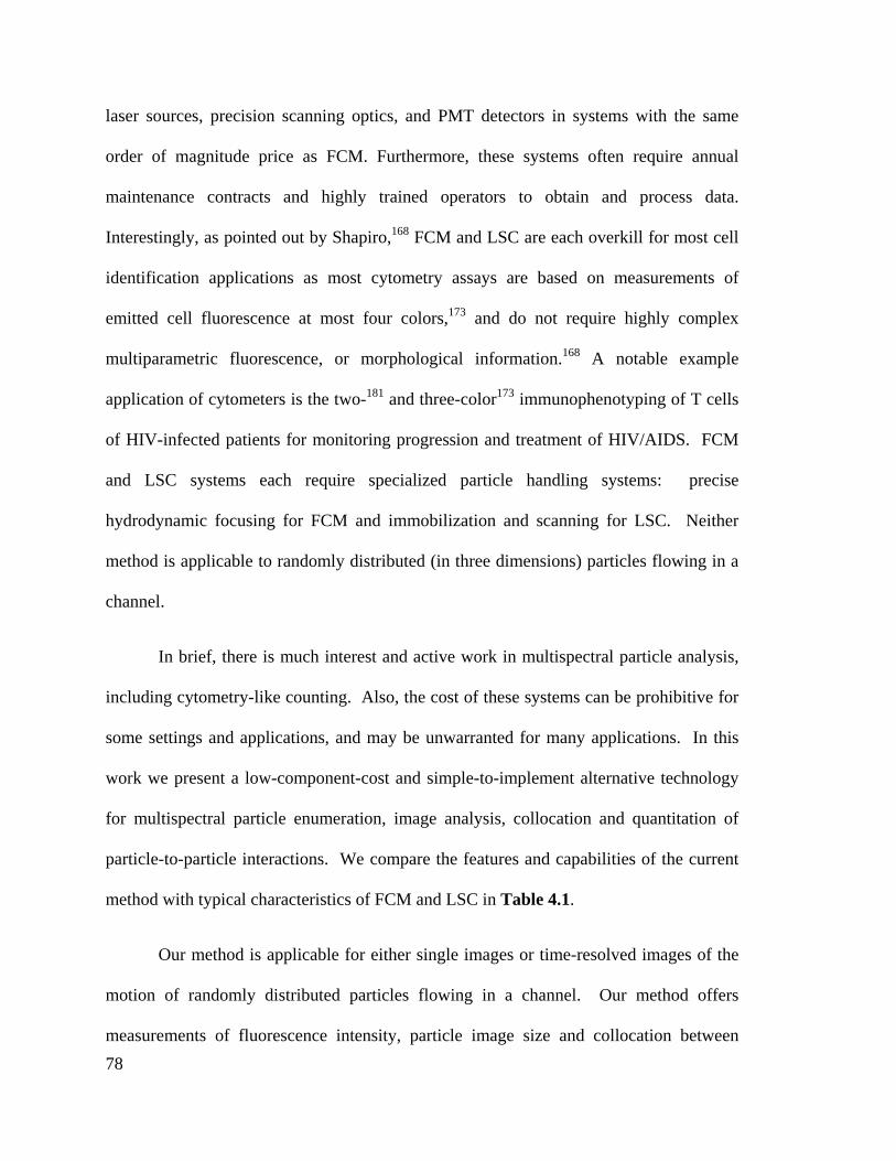
78

laser sources, precision scanning optics, and PMT detectors in systems with the same

order of magnitude price as FCM. Furthermore, these systems often require annual

maintenance contracts and highly trained operators to obtain and process data.

Interestingly, as pointed out by Shapiro,168 FCM and LSC are each overkill for most cell

identification applications as most cytometry assays are based on measurements of

emitted cell fluorescence at most four colors,173 and do not require highly complex

multiparametric fluorescence, or morphological information.168 A notable example

application of cytometers is the two-181 and three-color173 immunophenotyping of T cells

of HIV-infected patients for monitoring progression and treatment of HIV/AIDS. FCM

and LSC systems each require specialized particle handling systems: precise

hydrodynamic focusing for FCM and immobilization and scanning for LSC. Neither

method is applicable to randomly distributed (in three dimensions) particles flowing in a

channel.

In brief, there is much interest and active work in multispectral particle analysis,

including cytometry-like counting. Also, the cost of these systems can be prohibitive for

some settings and applications, and may be unwarranted for many applications. In this

work we present a low-component-cost and simple-to-implement alternative technology

for multispectral particle enumeration, image analysis, collocation and quantitation of

particle-to-particle interactions. We compare the features and capabilities of the current

method with typical characteristics of FCM and LSC in Table 4.1.

Our method is applicable for either single images or time-resolved images of the

motion of randomly distributed particles flowing in a channel. Our method offers

measurements of fluorescence intensity, particle image size and collocation between

79

multiple colors. The latter helps monitor particles which emit at multiple wavelengths

and particle-to-particle type interactions. One unique feature of our technique is that it

can monitor the time evolution of particle-particle interactions (we demonstrate evolution

times of ~8 s, but this can be increased by changing flow and/or imaging conditions).

Further, our image analysis can handle suspensions with particle densities in excess of

108 mL-1 (by comparison, FCM require densities of 106 mL-1 or less). All of the analysis

can be performed in a suspension flow inside virtually any microchannel or tube with

optical access for particle imaging (e.g., off-the-shelf microfluidic chips). Here we

demonstrate a version of our technique optimized for analyzing specific particle-to-

particle interactions and the resulting collocation and correlation of particle image

motions.

Table 4.1. Brief review and comparison of multispectral particle analysis and enumeration techniques. We

compare the capabilities and features of the current technique (PITC) with FCM and LSC.

FCM LSC PITC

Cost High High Low

Particle matrix Hydrodynamically focused suspension

Fixed onto a slide surface

Flowing, random suspension

Multi-particle visualization No No Yes Spatially-resolved particle images No Yes Yes Number of measurements per particle One Several 5-20+ Time-resolved particle analysis No Yes Yes Particle-to-particle interactions No Yes Yes Particle rate 100-50,000 s-1 Up to 100 s-1 Up to 1000 s-1 Spatial resolution Low High Moderate

Recommended particle concentration Up to 106 mL-1 109 mL-1 Up to 108 mL-1

Minimum sample vol. required Order 100 µl Order 1 ul Order 10 µl

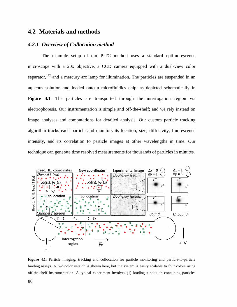
80

4.2 Materials and methods

4.2.1 Overview of Collocation method

The example setup of our PITC method uses a standard epifluorescence

microscope with a 20x objective, a CCD camera equipped with a dual-view color

separator,182 and a mercury arc lamp for illumination. The particles are suspended in an

aqueous solution and loaded onto a microfluidics chip, as depicted schematically in

Figure 4.1. The particles are transported through the interrogation region via

electrophoresis. Our instrumentation is simple and off-the-shelf; and we rely instead on

image analyses and computations for detailed analysis. Our custom particle tracking

algorithm tracks each particle and monitors its location, size, diffusivity, fluorescence

intensity, and its correlation to particle images at other wavelengths in time. Our

technique can generate time resolved measurements for thousands of particles in minutes.

Figure 4.1. Particle imaging, tracking and collocation for particle monitoring and particle-to-particle

binding assays. A two-color version is shown here, but the system is easily scalable to four colors using

off-the-shelf instrumentation. A typical experiment involves (1) loading a solution containing particles

81

emitting in the red and green into a microchannel; (2) electrophoresing the particles through a detection

region with optical access; and (3) imaging at a user-specified rate using a microscope equipped with dual-

view system and high-sensitivity CCD camera. The dual-view system chromatically separates the particle

images into separate spatial domains on the CCD array. The PITC algorithm determines location and in-

plane velocity vectors of each particle in one spectral channel. This analysis is used to track the

coordinates, image size, and fluorescence intensity of the individual particles in time. The subregions

surrounding the particles in channel 1 are identified and tracked then cross-correlated with the

corresponding subregions in the other channel. The persistence (in time) of a high cross-correlation signal

indicates deterministically bound particles.

4.2.2 Reagents and materials

We purchased 1.0 µm carboxylate-modified FluoSpheres® microspheres

(625/645), and 1.0 µm carboxylate-modified FluoSpheres® microspheres (505/515)

manufactured by Molecular Probes, Life Technologies. The red bead was conjugated

with 5’- Amino Modifier C12 – CGGATTGGAGTCTGCAACTCG and the green bead

with 5’- Amino Modifier C12- CACAAAGTGGTAAGCGCCCTC. The conjugation

reactions were performed by Radix Biosolutions (Georgetown, TX), and beads were

suspended in Tris-EDTA, pH 8 at 2% solids. The functionalized beads were mixed with

the target, a sequence that corresponds to a region in the E.coli 16S rRNA transcript:

AAACGAGTTGCAGACTCCAATCCGAAAAGAAGTAGGTAGCTTAACCTTCGGG

AGGGCGCTTACCACTTTGTGTTT

The hybridization buffer contained 20 mM Tris, 10 mM hydrochloric acid, HCl, 0.08%

Triton X-100 and 50 mM sodium chloride, NaCl. Reagents Tris, HCl, Triton X-100 and

NaCl were purchased from Sigma-Aldrich (St. Louis, MO). The DNA was synthesized

by Integrated DNA technologies, (IDT, Coralville, IA). The bead probes were desalted

and the target sequence was PAGE purified. The buffered bead suspension was first

82

mixed with 100 nM target DNA in presence of 3x109 beads/mL of each color and

incubated at 60°C for 1 min followed by 50°C incubation for 10 min. The solution was

diluted 10-fold with the hybridization buffer and pressure loaded into a poly(methyl

methacrylate) microfluidic chip channel with dimensions 2 x 0.15 x 100 mm (Figure

4.2). The output well was filled with 50 µl of 1 M Tris-HCl buffer. The loading well was

filled with the same buffer containing 25% Pluronic F-127 solution in order to reduce

pressure driven flow. Platinum electrodes were placed in the loading and output wells and

electrophoresis was initiated by applying a constant current of 100 µA. The bead

suspension is imaged using an Olympus IX70 microscope equipped with a 20x, NA = 0.5

Olympus UPlanFl objective, a 16-bit CCD (Cascade 512F) camera (520 x 520 of 16 µm

pixels). We achieved spatial separation of two wavelengths using an XF53 dual pass filter

cube (Omega Optical) with peak excitation wavelength ranges of 475–500 and 550–600

nm, and peak emission wavelength ranges of 500–550 and 600–675 nm, in combination

with a quad-view imager (Micro-Imager, Photometrics, Tucson, AZ). (Used here in dual-

view mode for simple demonstration.) In a typical experiment, we record 200 images of

particles illuminated with a mercury light source for 5 ms at a frequency of 1 Hz. During

this time, order 1,000-10,000 unique beads traverse through the field of view. The

particle motion and imaging rate can be increased for applications requiring higher

throughput and where particles or cells require shorter evolution period monitoring.

83

Figure 4.2. Fluidic channel architecture and loading protocol used in demonstration of particle imaging,

tracking and collocation method. A poly(methyl methacrylate), PMMA, microfluidic fluidic chip with

dimensions (10 cm x 2 mm x 150 µm) is loaded with the buffered bead suspension. The output well was

filled with 50 µl of 1 M Tris-HCl (pH 8) buffer. The loading well was filled with the same buffer

containing 25% Pluronic F-127 solution in order to reduce pressure driven flow. Platinum electrodes were

placed in the loading and output well and electrophoresis was initiated by applying 100 µA across the

microchannel. In a typical experiment, we record 200 chromatically separated particle images at a

frequency of 1Hz. During this time, order 1,000-10,000 unique beads traverse through the field of view.

We note here that most biological laboratories already have access to

epifluorescence microscopes and CCD cameras. Our method requires only a CCD camera

with fairly good sensitivity and imaging rates of about 1 frame per second or higher. We

also require an off-the-shelf dual- or quad-view type image splitter. The dual-view

imager and filter set for two-color imaging is currently available for $11,000, while a

quad-view (for four color imaging) is available for $19,000. We believe our method is

amenable to further lowering component cost.

4.2.3 Imaging and particle residence time requirements

Our algorithm relies on particle brightness patterns, and so we recommend

imaging conditions such that particle image diameters correspond to distances of 3 or

more pixels (roughly 3 to 8 pixels is ideal). To discriminate between bound and closely

neighboring particles we can monitor the persistence (in time) of the spatial correlation of

84

particle images. This option places a minimum requirement on the amount of time the

algorithm tracks particles. The algorithm should track particles long enough for Brownian

motion or other dispersion to cause separation of unbound particles. For particle

separation phenomena determined by Brownian motion, we can estimate this minimum

time of observation from particle diffusivity. For particles with radius, rp, and particle

image radius (geometrically projected into the object plane), rpi, we recommend the

following relation to estimate the minimum time, tch, over which to track particle pairs

undergoing Brownian diffusion:

( ) ( )[ ]),min(4/54 2,1,2,1, pipippcheffch rrrrtDL ++>= . (4.1)

Here, Lch is a characteristic minimum particle center-to-center distance in object space,

required before the algorithm concludes the particles are not bound. At the characteristic

time, tch, diffusion statistics183 suggest that 67% of all randomly aligned particles pairs

with effective diffusivity of Deff, are separated by Lch. We estimate the Brownian

separation distance between two particles using an effective diffusion coefficient of the

form Deff = Dp1 + Dp2, where Dp1 and Dp2 are respectively the diffusivities of particles

imaged in channels 1 and 2. Here we assume that the diffusive motions of the closely-

spaced particles are statistically independent.183 Combining equation (4.1) with the

Einstein diffusivity expression,184 pp rkTD πµ32= , we can solve for the characteristic

minimum evolution time:

( )( )

+

++=

2,1,

22,1,1,1,

112

),min(4/5)(3

pp

pipippch

rrkT

rrrrt

πµ (4.2)

85

In our experiments, this time is roughly 2.5 s. Appropriate choices for monitoring time

are discussed further in the ‘Validation and Performance’ section.

So far, we focused on the point-to-point lateral resolution and separation distance

in the plane perpendicular to the optical axis. Another important consideration is the

depth of field, LDf , which is determined by the distance from the nearest object plane in

focus to that of the farthest plane. In microscopy depth of field is very short and it is

determined only by the numerical aperture of the objective. In general, high numerical

aperture systems have higher magnification power. For particle tracking and colocation

analysis, we recommend choosing imaging conditions that ensures that the tracked

particle hybrids remain in focus for the minimum required elution time. This condition is

met if the depth of field is larger than the characteristic length,

( ) ( )2,1,2,1, ,min)4/5( pipippf rrrrD ++> . This requirement can place a constraint on the

maximum magnification power of the optical train. When higher resolving power is

required, alternative means to keep particles is focus may be necessary.

4.2.4 Particle tracking and collocation algorithm

Figure 4.3 shows an overview of our PITC algorithm, which we implemented on

MATLAB (Mathworks Inc., Natick, MA). We first spatially register the two spectral

channels using a bright field image of an alignment mask. The algorithm is then divided

into two phases. In the first phase, we analyze particle images from one spectral channel

(Channel 1) to identify and track particle coordinates, size and fluorescence. In the

second phase, we perform collocation, which analyzes the region in the second channel

images (Channel 2) which are immediately near particles identified in the first channel.

86

The process can be performed twice with the first phase starting with each of the two

channels. This enables counting and tracking particles individually in each channel and

corroboration of the collocation analysis. For the current demonstration, the algorithm is

performed as a post-process routine but the process is amenable to parallelization and

real-time implementation. In the following sections, we provide details of the particle

tracking and particle collocation phases.

Figure 4.3. PITC algorithm structure. Each image sequence contains data for thousands of unique

particles. After registration of the two images, the algorithm proceeds in two main phases. The first phase

quantifies local drift particle velocities using micron resolution particle image velocimetry (micro-PIV).

Unique particle images in Channel 1 (Ch1) are then identified, located and characterized via the particle

mask correlation and particle characterization (PMC-PC) method. The particle image intensity and radius

are evaluated using a non-linear Gaussian fitting routine. The algorithm then combines results of PMC-PC

and micro-PIV for a particle tracking velocimetry (PTV) subroutine enhanced by Kalman filter and χ2-

testing method (KC-PTV). This analysis results in accurate determination and tracking of the location of

each particle over time and space. The second phase of the algorithm cross-correlates subregions

surrounding the particle locations identified in Ch1 with corresponding subregions in the registered Ch2.

Ch2 particle characteristics, such as radius and total fluorescence, are evaluated using the Gaussian fitting

87

subroutine. Thresholds for intensity, size, velocity, and correlation coefficient are applied at each step to

eliminate spurious results.

Alignment and spatial registration

We spatially register the two channel images using a bright field image of an

alignment pattern (Negative 1951 wheel pattern resolution test target from Thorlabs,

R3L1S4N). Example misaligned (initial) and aligned (final) versions of this test pattern

are shown in Figure 4.4. We used Matlab’s function imregister, an iterative process that

requires a pair of images, an image-similarity metric, an optimizer, and a transformation

type. The metric defines the image similarity for evaluating the accuracy of the

registration. The optimizer defines the methodology for minimizing or maximizing the

similarity metric.

Figure 4.4. Example of misaligned (initial) and aligned (final) bright-field images of two spectral channels

recorded with a quad-view imager (Micro-Imager, Photometrics, Tucson, AZ), used here in dual-view

mode. The images are plotted using Matlab’s function, imshowpair, which displays the differences between

two images. We used alpha blending to overlay the two spectral channel images before (left) and after

(right) image registration. Note, alpha blending is the process of combining a translucent foreground color

with a background color, which produces a new blended color. These test images were taken with a 20x

objective with a numerical aperture of 0.5.

88

We used Matlab’s function imconfig to generate the optimizer and metric assuming

multimodal image capture, as the brightness range in the two spectral channels are

different. The transformation type used for the image alignment is specified as “rigid”,

which consists of translation, and rotation. We set the maximum iterations to 1000. The

ROI coordinates and the transformation matrix generated in this alignment phase are then

used to translate and rotate the Ch2 particle image to achieve spatial registration with

Ch1. Using images of simulated particle patterns; we have verified that this alignment

procedure results in registration with sub-pixel accuracy. Note, the image alignment and

registration process will produce artifacts at the perimeter of the images, which are

eliminated by trimming ~ 5 pixels from the image edges. This entire process needs to be

performed only periodically as a part of the instrumentation calibration procedure.

Particle tracking phase (Channel 1)

Micron-resolution Particle Image Velocimetry

We use measurements of spatially correlated particle motion (i.e., velocities

averaged over finite subregions containing multiple particles) to guide our individual

particle tracking algorithm. This correlated particle motion is the result of non-Brownian

transport such as fluid flow or electrophoresis or both. micro-PIV provides a robust and

high-resolution method for determining such spatially correlated particle velocities.185

micro-PIV was developed specifically for microfluidic applications, and has been

reviewed and described extensively.186-188 The process limits particle tracking to particles

near the focal plane of epifluorescence imaging.188 The process measures two

components (x- and y-velocities) of the velocity field in the imaging plane. For our

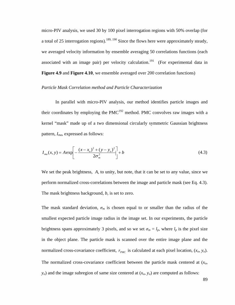
89

micro-PIV analysis, we used 30 by 100 pixel interrogation regions with 50% overlap (for

a total of 25 interrogation regions).189, 190 Since the flows here were approximately steady,

we averaged velocity information by ensemble averaging 50 correlations functions (each

associated with an image pair) per velocity calculation.191 (For experimental data in

Figure 4.9 and Figure 4.10, we ensemble averaged over 200 correlation functions)

Particle Mask Correlation method and Particle Characterization

In parallel with micro-PIV analysis, our method identifies particle images and

their coordinates by employing the PMC192 method. PMC convolves raw images with a

kernel “mask” made up of a two dimensional circularly symmetric Gaussian brightness

pattern, Ima, expressed as follows:

byyxxAyxIm

ooma +

−+−−= 2

22

2)()(exp),(

σ (4.3)

We set the peak brightness, A, to unity, but note, that it can be set to any value, since we

perform normalized cross-correlations between the image and particle mask (see Eq. 4.3).

The mask brightness background, b, is set to zero.

The mask standard deviation, σm is chosen equal to or smaller than the radius of the

smallest expected particle image radius in the image set. In our experiments, the particle

brightness spans approximately 3 pixels, and so we set σm = lp, where lp is the pixel size

in the object plane. The particle mask is scanned over the entire image plane and the

normalized cross-covariance coefficient, PMCr is calculated at each pixel location, (xo, yo).

The normalized cross-covariance coefficient between the particle mask centered at (xo,

yo) and the image subregion of same size centered at (xo, yo) are computed as follows:

90

( ) ( )∑ ∑∑ ∑

∑ ∑+

−=

+

−=

+

−=

+

−=

+

−=

+

−=

−−

−−=

2/

2/

2/

2/

22/

2/

2/

2/

2

2/

2/

2/

2/

ˆ),(ˆ),(

)ˆ),()(ˆ),((),(

mx

mxi

ny

nyjmama

mx

mxi

ny

nyj

mx

mxi

ny

nyjmama

ooPMCo

o

o

o

o

o

o

o

o

o

o

o

IjiIIjiI

IjiIIjiIyxr (4.4)

where I(i,j) is the brightness value of particle image plane at (i,j).192 In this study, we set

the particle mask size (n,m) to 8σm x 8σm. PMCr varies between -1 to 1, depending on the

degree of similarity between the brightness patterns. Pixels with high covariance

coefficients indicate the presence of particles. Using a covariance threshold of 0.7 enables

the PMC method to find all concentric convex brightness patterns of size of roughly < 8

σm.192 The calculated covariance coefficient plane is binarized using this threshold. For

simplicity, we assign the pixel with the highest PMCr value as the coordinate for the center

of the particle, (xp,1,yp,1). As an approximation, we evaluate the particle image radius

(geometrically projected into the object plane) as ( ) π/21, ppi plr = , where p is the

number of ‘unity’ pixels for a particle group in the binarized image, and lp is the size of

the pixel in the object space. While the cross-covariance was performed on raw particle

images, the particle intensity, Ip,1, is estimated by summing the background corrected

intensity of a 4rpi,1 x 4rpi,1 subregion centered at the particle center (xp,1, yp,1). The

corrected images are evaluated as follows:

flat

bgrawc I

III

−= . (4.5)

The background of the raw image, Ibg is obtained by filtering the original image with a

median filter of size 10x10. The flatfield, Iflat, is obtained by imaging the microchannel

91

filled with uniform concentration of dyes (100 nM AF488 and 100nM AF647) which are

processed with a median filter of size 10x10.

We note that our method can significantly improve the accuracy of particle

localization and size and fluorescence characterization by using a sub-pixel resolution

method. The sub-pixel resolution approach fits the particle brightness pattern in the local

8σm x 8σm subregion of background corrected particle image using a non-linear Gaussian

fitting routine. The brightness pattern is defined by Eq. 4.3, where we set the standard

deviation equal to the particle image radius, σm = rpi,1. The fitting routine uses the median

intensity of the 8σm x 8σm subregion as the background, b; the highest pixel intensity

minus the background as the amplitude, A; and the simple estimates, described above, for

particle coordinates and particle radius for xp,1, yp,1 and rpi,1, as a first guess. We used and

recommend the fitting routine for more detailed cytometry-like data of particle

populations. For the simulated particle-to-particle binding assay data we present in

Figure 4.6 and Figure 4.7 below, we disabled this Gaussian fitting algorithm step in

order to save computational time.

To eliminate large aggregates and out-of-focus particles from analysis, we

implemented size- and intensity-based threshold filters. For the particle-to-particle

collocation analysis presented in this study (unless stated otherwise), we set the size-

based threshold to eliminate particles with radii larger than the mean plus 2 times the

standard deviation of the particle population in each image. The intensity-based threshold

eliminated all features with intensity 3 times the standard deviation away from the mean

of the particle population.

92

Kalman filter and χ2-test enhanced Particle Tracking Velocimetry

For robust and accurate operation, we us Kalman filter and χ2-test192, 193 to

identify and track each unique particle over time and space. This latter method, KC-PTV,

was developed by Etoh and Takehera for particle tracking velocimetry.192, 194 KC-PTV

was later adapted for microfluidics by incorporating micro-PIV.195, 196 In KC-PTV,

particle image data (here location, fluorescence intensity, and particle image radius) from

the first time step (t = 0) is used to predict the particle information in the next time step (t

= t+∆t). The probability of two particle images belonging to the same particle identity is

evaluated using a χ2-test which uses these image data as parameters. See work by

Takehara and co-workers192, 193 for more detailed information on the implementation of

the approach.

In this phase of our algorithm, we apply filters to the data which reject particle

image motions which are significantly far from bounds determined by local micro-PIV

velocity data and particle diffusion estimates. For example, we reject particle matches

with apparent velocities, apv , , which fail the following criteria:

),(5 1,1,, ppPIVapdiff yxvvv −> . Here, tDv pdiff ∆= 4 , and ),( jivPIV is the drift velocity at

the particle position (xp,1,yp,1) obtained from micro-PIV analysis. Output parameters from

this phase, including particle identification number (ID), coordinates, xp1(t), yp1(t),

particle image radius, rpi,1(t), and integrated background-corrected fluorescence intensity,

Ip(t), are stored for further processing.

93

Particle collocation phase from Channel 1 and 2 data

Our particle collocation approach begins by positioning a small 8σm x 8σm

subregion at the coordinates of each particle identified and tracked in Ch1. The algorithm

then selects a 16σm x 16σm subregion in Ch2 centered at the same coordinates. We limit

the shifts in correlations so that the Ch1 subregion always completely overlaps the Ch2

subregion, and so we eliminate the known biases associated with cross-correlations of

finite-sized correlation functions.189, 190 For the collocation analysis, we evaluate the

normalized cross-covariance as described by Eq. 4.4, but where we set Im to the Ch1

subregion and set I to the Ch2 subregion. The parameter PMCr is then interpreted as the

degree of correlation in the position of the particle or particles detected in both Ch1 and

Ch2, which we refer to as collocation coefficient, ),,(12 tyxR oo . ),,(12 tyxR oo is evaluated

for widow offsets of (xo, yo) equal to or less than a predefined minimum value,

( ) ( )2,1,2,1, ,min)4/1( pipipp rrrrSh ++= . We initially assign the offset (xo, yo) with the

highest ),,(12 tyxR oo value as the coordinate for the center of the Ch2 particle, (xp,2, yp,2).

If the maximum coefficient, max,12R , is below 0.6, we conclude that no particles are

present in Ch2 subregion. For such a case, we set 02, =pir and estimate Ip,2 as the sum of

the background corrected particle image intensity (Eq. 4.5) of a 4rpi,1 x 4rpi,1 subregion

centered at (xp,1, yp,1) in Ch2. If max,12R is above 0.6, we conclude that there is a particle in

the Ch2 subregion. To estimate the radius of the particle, we first binarize the collocation

matrix and find the group of unity pixels associated with the Ch2 particle coordinates

(xp,1, yp,1). We approximate the particle image radius (in object plane) as

( ) π/22, ppi plr = . Particle radius is subsequently used to determine the Ch2 particle

94

intensity, Ip,2, by summing the background corrected image intensity (Eq. 4.5) of a

4rpi,2 x 4rpi,2 subregion centered at (xp,2, yp,2).

Recall that the particle characterization method can significantly improve the

accuracy of particle localization, size and fluorescence characterization by using a sub-

pixel resolution method as described in the PMC subsection. We implement the non-

linear Gaussian fitting routine in data analysis presented in Figure 4.9 and Figure 4.10.

Interpreting collocation data

The persistence (in time) of a high cross-correlation signal indicates

deterministically bound particles. This is in contrast to unbound, but closely neighboring

particles, which eventually separate due to Brownian motion and/or dispersion. We

therefore identify particles as bound only if their collocation coefficient )(max,12 tR remains

sufficiently high for longer than a predefined minimum tracking time, tch determined

from Eq. 4.2. Particle image pairs in Ch1 and Ch2 with collocation traces, )(max,12 tR ,

with a median collocation value above a predefined threshold, 12~R , are determined to be

bound. Appropriate choices for median collocation thresholds are discussed in the

following section.

To prevent highly correlated, non-particle related events to contribute to bound

event counts, we have also implemented an intensity-based threshold filter, which

95

removes all collocated events with intensities 3 (for simulated) and 1 (for experimental

data) standard deviation away from the mean of the “bound” particle population.1

4.3 Validation and Performance

4.3.1 Monte Carlo simulations

We used Monte Carlo simulations to guide our choices of user specified algorithm

parameters and to demonstrate the performance and robustness of our particle collocation

algorithm. We first performed Monte Carlo simulations of Brownian particles with

Gaussian brightness patterns of one pixel standard deviation (see Figure 4.5 for example

images). The particles were randomly distributed in a 500 x 150 cell simulation domain

which corresponded to the pixel array. Particle diffusivity was set to 0.44 µm2/s, and the

particles were given a uniform advective velocity of vp,x = 10 µm/s. As typical with

Brownian Monte Carlo, we chose specular reflection boundary conditions for the side

walls of the simulation domain. Further, particles exiting the x = 150 end of the domain

were reintroduced at x = 0, at random y-coordinates. To explore the sensitivity of our

method to experimental conditions, we simulated the following variations: (1) percentage

of bound particles between the two channels ranged between 0-100%, (2) inter-particle

distance varied between 5 to 20 µm, and (3) image signal to noise ratio (SNR) ranged

between 2 to 100. Note, that the average inter-particle distance of nearest neighbor

particles can be determined as LIP=0.5539d-1/3,183 where d(m-3) is particle density. Inter-

1 We note here, that the effectiveness of these filters relies on access to accurate particle intensity and size distributions. For experiments where the fraction of bound particles are zero or exceptionally low, the intensity and size distribution of Ch2 particle images are biased from false positive collocation matches. For example, in a negative control experiment, most collocation matches are due to image artifacts. Therefore, the intensity and size characteristics of their distribution should not be used in these filters. We thus recommend the calibration of particle intensity and size via PMC-PC in Ch2 before collocation analysis.

96

particle distance of 5 to 20 µm is equivalent to about 800 to 50 particles in a 500 x 150

simulation domain.

4.3.2 Image SNR and median collocation threshold

The probability of successful particle identification and collocation rely strictly on

the degree of correlation between two normalized brightness patterns. Signal-to-noise

ratio (SNR) has a strong effect on the brightness pattern of raw particle images. We

define SNR as the peak particle intensity above the mean of local background divided by

2 times the standard deviation of background image intensity. To determine how SNR

influences particle tracking and collocation accuracy, we added Gaussian white noise to

the simulated particle fields (see Figure 4.5 for simulated images with SNR of 2 and

100). During the 200 s simulation time, we introduced 1422 of unique particles, 1200 of

which had a residence time of roughly 15 s. We performed particle tracking on the

simulated images and plot in Figure 4.5 the histogram of tracked particle times (duration

over which algorithm tracks each particle) as a function of SNR. In the case of low image

SNR (SNR = 2), over 200 s, approximately 5000 particles were identified, but only 10%

were tracked for 3 s or longer. Note, that when the algorithm loses a particle due to the

interfering effects of SNR, if the same particle reemerges at a later time step, it is

identified as a new particle (as would happen in an experiment). Consequently, the

number of particle counts increases, and residence time shortens with increasing image

noise. Consistent with this is the large discrepancy present between the number of

particles detected (~5000) and simulated (~1400) at SNR = 2. For image SNR of 5 or

above, the number of particles identified and their tracked time converges to the known

values.

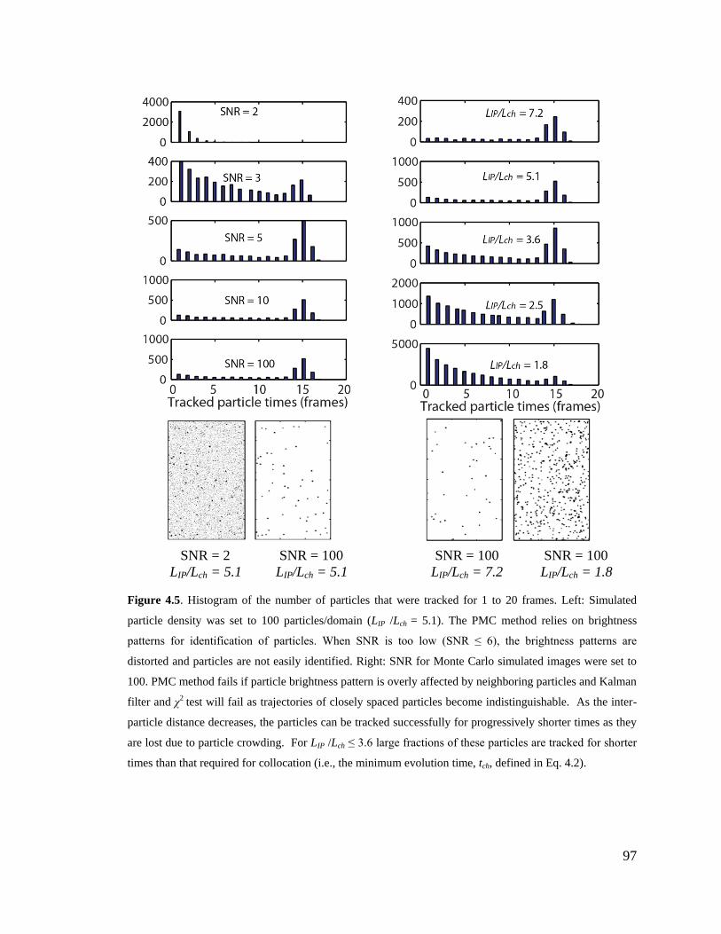
97

SNR = 2 LIP/Lch = 5.1

SNR = 100 LIP/Lch = 5.1

SNR = 100 LIP/Lch = 7.2

SNR = 100 LIP/Lch = 1.8

Figure 4.5. Histogram of the number of particles that were tracked for 1 to 20 frames. Left: Simulated

particle density was set to 100 particles/domain (LIP /Lch = 5.1). The PMC method relies on brightness

patterns for identification of particles. When SNR is too low (SNR ≤ 6), the brightness patterns are

distorted and particles are not easily identified. Right: SNR for Monte Carlo simulated images were set to

100. PMC method fails if particle brightness pattern is overly affected by neighboring particles and Kalman

filter and χ2 test will fail as trajectories of closely spaced particles become indistinguishable. As the inter-

particle distance decreases, the particles can be tracked successfully for progressively shorter times as they

are lost due to particle crowding. For LIP /Lch ≤ 3.6 large fractions of these particles are tracked for shorter

times than that required for collocation (i.e., the minimum evolution time, tch, defined in Eq. 4.2).

98

In Figure 4.6, we show the combined accuracy of particle tracking and

collocation as a function SNR and collocation median threshold, 12~R for two different

simulation fractions of bound particles. For both cases of 3% and 50% bound particles,

increasing image SNR improves collocation accuracy. In general, strong image noise

results in an underestimation of the bound fraction. Of the severest of cases, SNR = 2, no

bound particles were detected for any collocation thresholds in the tested range (

8.06.0~12 −=R ). The collocation results for images with SNR of three, using threshold of

6.0~12 =R are in close agreement with the simulated values, but raising 12

~R to 0.8, causes

complete failure of the collocation analysis. For SNR > 5, the collocation accuracy is

weakly dependent of SNR and collocation thresholds. For example, prediction of PITC

analysis of the 3% bound fraction case (solid line) at SNR = 10, is 2.91%, when

6.0~12 =R and 2.64%, when 8.07.0~

12 −=R . Based on these analyses, we determined that

a value of 6.0~12 =R yields an appropriate accuracy for a fairly wide range of image SNR.

In the inset of Figure 4.6, we also show the results of collocation performed on

image sets with 0% simulated bound particle fraction. At image SNR = 100, the PITC

algorithm found that bound particle doublets made up 0.9%, 0.6%, and 0.25% of the total

particles with collocation threshold values of 0.6, 0.7 and 0.8, respectively. False

positive collocation detections occur in the negative control case due to failure of the

particle intensity threshold filter we implemented in the collocation phase. This intensity

based threshold relies on the intensity distribution of true positive particle matches in

Ch2. Since there are no true positive matches in the negative control case, the intensity

distribution obtained this way is not a true representation of the Ch2 particle intensities.

99

These bound fractions in Figure 4.6 inset, therefore, represent the limit of detection

(LOD) of our method in the absence of a priori Ch2 particle intensity calibration. To

improve the LOD, we recommend the evaluation of particle intensities in Ch2 using the

PMC-PC method. The calibrated intensity distribution can then be used to filter particle

matches in the collocation phase. After we performed a simple calibration of Ch2

particles, the PITC algorithm detected 0% bound fractions for all collocation thresholds

in the negative control case.

Figure 4.6. Accuracy of particle hybrid count as a function of simulated SNR and the median collocation

threshold, 12~R . The total number of 1 μm diameter particles in each image from the Monte Carlo

simulation is 100 (with a mean inter-particle distance of roughly 15 μm). The simulated fraction of bound

versus total particle number was 0% (inset), 3% (solid line) and 50% (dashed line). Particles were

considered only if they were tracked for 10 s or longer. For the tested range of collocation thresholds, the

bound particle fraction is underpredicted. For the highest collocation threshold of 0.8, PITC detected no

bound particles for SNR < 5. As SNR increases above 5, the detected bound fraction converges to the

simulated values. In inset, we show 0.9%, 0.5% and 0.3% false positive bound fraction detected in the

negative control case for the three collocation threshold values. The false positive bound fraction is reduced

to 0% for all 12~R , when Ch2 particle intensity distribution (calibrated Ch2 particle intensity) is used as the

basis of the intensity-based filter in the collocation phase.

100

4.3.3 Particle density and monitoring time

The rate of particle analysis of our collocation method is primarily limited by two

parameters, the maximum particle concentration tolerated by the PITC algorithm and the

minimum monitoring time, tm. Here we examine the effect of these parameters on particle

tracking and collocation performance. We analyzed image pairs containing 50, 100, 200,

400 and 800 particles per image, 3% of which were deterministically bound. During the

200 s simulation time, we introduced 718, 1437, 2851, 5692 and 11314 unique particles,

most of which had a residence time (time spent in the field of view) of roughly 15 s. In

Figure 4.5 of the SI, we show a histogram of particle tracked times as a function of

particle density. High particle density is associated with short inter-particle distances.

Since neighboring particles influence the brightness pattern of those that are tracked, the

success rate of particle tracking decreases with increasing particle density. For image sets

containing 200 or more particles, the tracked times are limited by particle crowding, and

not by the user specified parameters such velocity and interrogation widow-size. For

example, for the highest particle density case (800/image), most particles can be tracked

for at most 5 s.

In Figure 4.7, we elucidate the influence of particle density on collocation

performance by comparing the inter-particle distance, LIP, to the characteristic distance

that two randomly aligned particles must separate for the algorithm to consider them

unbound, Lch (Eq.4.4). Here we also examine the influence of monitoring time, tm on

collocation by comparing tm to the minimum elution time, tch (Eq. 4.2), the characteristic

time it takes two randomly bound particles to separate by Lch. Figure 4.7 shows the ratio

between the evaluated and simulated bound fraction as a function of LIP/Lch and tm/tch,

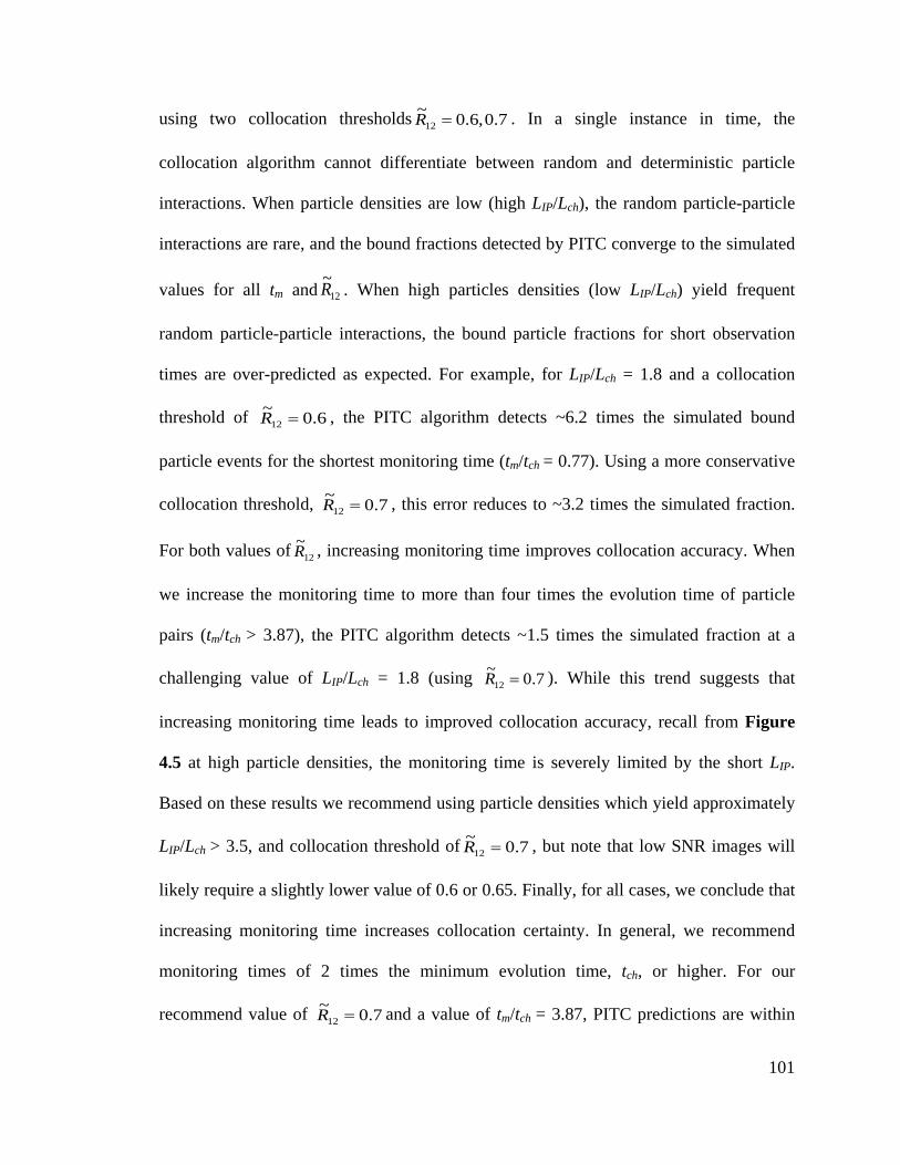
101

using two collocation thresholds 7.0,6.0~12 =R . In a single instance in time, the

collocation algorithm cannot differentiate between random and deterministic particle

interactions. When particle densities are low (high LIP/Lch), the random particle-particle

interactions are rare, and the bound fractions detected by PITC converge to the simulated

values for all tm and 12~R . When high particles densities (low LIP/Lch) yield frequent

random particle-particle interactions, the bound particle fractions for short observation

times are over-predicted as expected. For example, for LIP/Lch = 1.8 and a collocation

threshold of 6.0~12 =R , the PITC algorithm detects ~6.2 times the simulated bound

particle events for the shortest monitoring time (tm/tch = 0.77). Using a more conservative

collocation threshold, 7.0~12 =R , this error reduces to ~3.2 times the simulated fraction.

For both values of 12~R , increasing monitoring time improves collocation accuracy. When

we increase the monitoring time to more than four times the evolution time of particle

pairs (tm/tch > 3.87), the PITC algorithm detects ~1.5 times the simulated fraction at a

challenging value of LIP/Lch = 1.8 (using 7.0~12 =R ). While this trend suggests that

increasing monitoring time leads to improved collocation accuracy, recall from Figure

4.5 at high particle densities, the monitoring time is severely limited by the short LIP.

Based on these results we recommend using particle densities which yield approximately

LIP/Lch > 3.5, and collocation threshold of 7.0~12 =R , but note that low SNR images will

likely require a slightly lower value of 0.6 or 0.65. Finally, for all cases, we conclude that

increasing monitoring time increases collocation certainty. In general, we recommend

monitoring times of 2 times the minimum evolution time, tch, or higher. For our

recommend value of 7.0~12 =R and a value of tm/tch = 3.87, PITC predictions are within

102

~10% or less for SNR = 100, for the case of only 3% particles bound (bound fraction is

estimated between 2.7% - 3.3%).

Based on the aforementioned study of the influence of LIP/Lch, we recommend

using particle densities which yield approximately LIP/Lch > 3.5, and a collocation

threshold of 7.0~12 =R . We note that images with SNR of less than about 5 will likely

require a slightly lower value of 12R (say 0.6 or 0.65). In general, we recommend

monitoring times of 2 times the minimum evolution time, tch, or higher.

Figure 4.7. Accuracy of particle hybrid count as a function of particle density, monitoring time, and

collocation threshold. The simulated fraction of bound particles was set to 3%, and the image SNR to 100.

For all collocation thresholds, as the inter-particle distance decreases, the frequency of random particle-

particle interaction increase. As a result, the algorithm overestimates the bound particle fraction. While the

accuracy of collocation improves by increasing the monitoring time, tm, and increasing collocation

threshold, 12~R from 0.6 to 0.7, the error in the detected fraction for LIP/Lch < 3 is still significant. At LIP/Lch =

1.8, 7.0~12 =R , and tm/tch = 3.87, PITC detects 4.5% bound. Using the same algorithm settings on image sets

with lower particle density, PITC detects 3.23%, 2.87 % and 3.06% bound particle fractions at LIP/Lch of

3.6, 5.1 and 7.2, respectively.

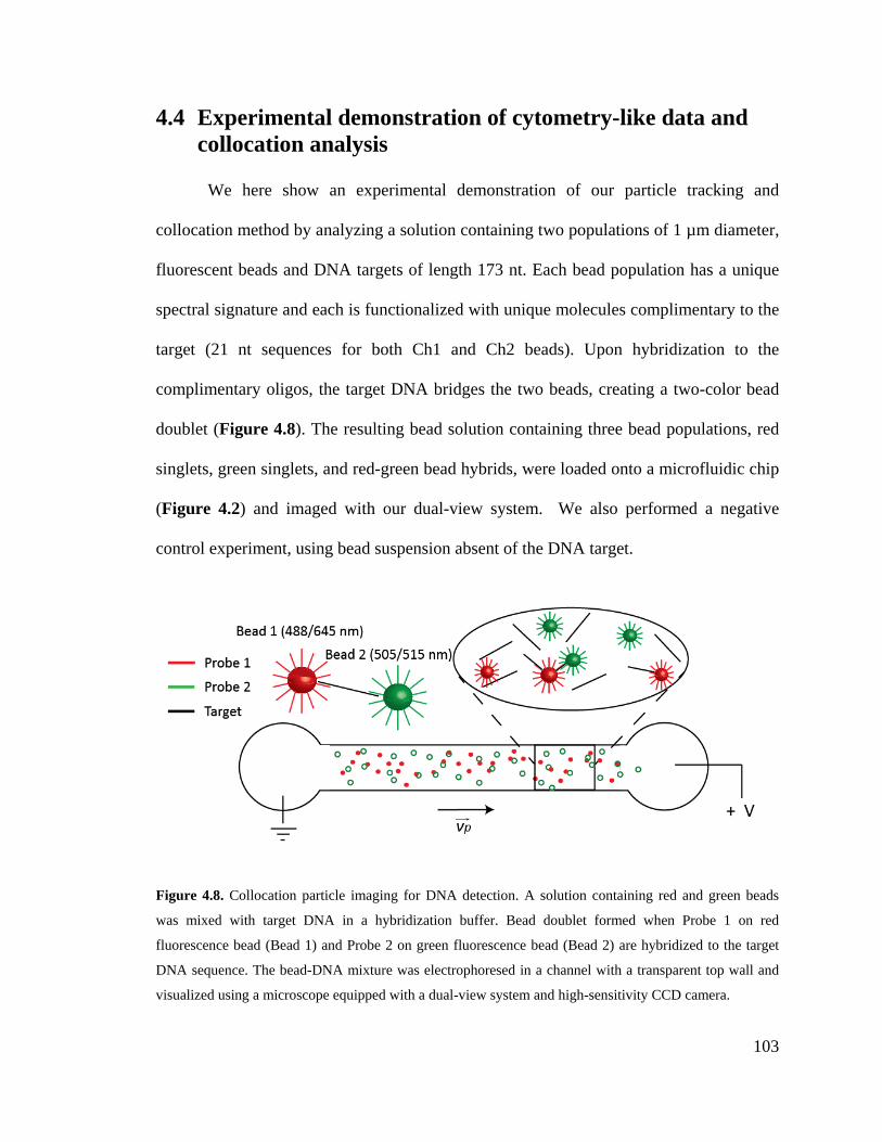
103

4.4 Experimental demonstration of cytometry-like data and collocation analysis

We here show an experimental demonstration of our particle tracking and

collocation method by analyzing a solution containing two populations of 1 µm diameter,

fluorescent beads and DNA targets of length 173 nt. Each bead population has a unique

spectral signature and each is functionalized with unique molecules complimentary to the

target (21 nt sequences for both Ch1 and Ch2 beads). Upon hybridization to the

complimentary oligos, the target DNA bridges the two beads, creating a two-color bead

doublet (Figure 4.8). The resulting bead solution containing three bead populations, red

singlets, green singlets, and red-green bead hybrids, were loaded onto a microfluidic chip

(Figure 4.2) and imaged with our dual-view system. We also performed a negative

control experiment, using bead suspension absent of the DNA target.

Figure 4.8. Collocation particle imaging for DNA detection. A solution containing red and green beads

was mixed with target DNA in a hybridization buffer. Bead doublet formed when Probe 1 on red

fluorescence bead (Bead 1) and Probe 2 on green fluorescence bead (Bead 2) are hybridized to the target

DNA sequence. The bead-DNA mixture was electrophoresed in a channel with a transparent top wall and

visualized using a microscope equipped with a dual-view system and high-sensitivity CCD camera.

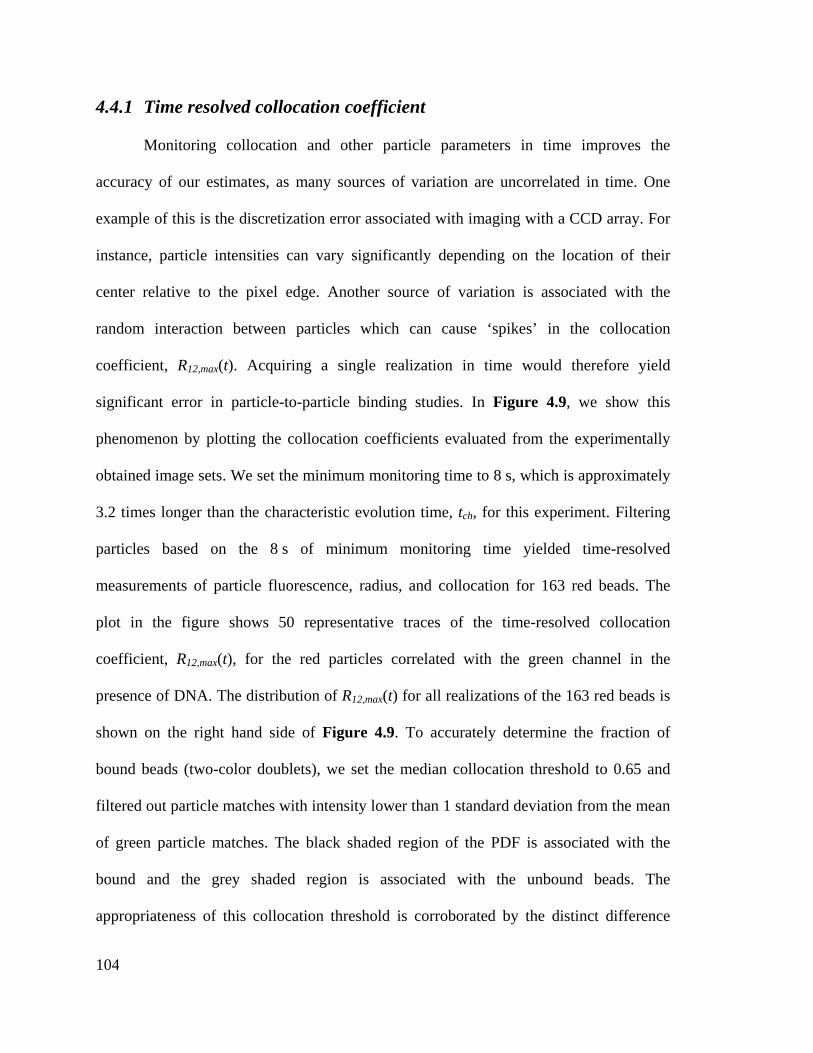
104

4.4.1 Time resolved collocation coefficient

Monitoring collocation and other particle parameters in time improves the

accuracy of our estimates, as many sources of variation are uncorrelated in time. One

example of this is the discretization error associated with imaging with a CCD array. For

instance, particle intensities can vary significantly depending on the location of their

center relative to the pixel edge. Another source of variation is associated with the

random interaction between particles which can cause ‘spikes’ in the collocation

coefficient, R12,max(t). Acquiring a single realization in time would therefore yield

significant error in particle-to-particle binding studies. In Figure 4.9, we show this

phenomenon by plotting the collocation coefficients evaluated from the experimentally

obtained image sets. We set the minimum monitoring time to 8 s, which is approximately

3.2 times longer than the characteristic evolution time, tch, for this experiment. Filtering

particles based on the 8 s of minimum monitoring time yielded time-resolved

measurements of particle fluorescence, radius, and collocation for 163 red beads. The

plot in the figure shows 50 representative traces of the time-resolved collocation

coefficient, R12,max(t), for the red particles correlated with the green channel in the

presence of DNA. The distribution of R12,max(t) for all realizations of the 163 red beads is

shown on the right hand side of Figure 4.9. To accurately determine the fraction of

bound beads (two-color doublets), we set the median collocation threshold to 0.65 and

filtered out particle matches with intensity lower than 1 standard deviation from the mean

of green particle matches. The black shaded region of the PDF is associated with the

bound and the grey shaded region is associated with the unbound beads. The

appropriateness of this collocation threshold is corroborated by the distinct difference

105

between the bound (solid) and unbound (dashed) collocation traces. Each of the bound

traces has a high mean (and high median) value in time with a narrow variance,

indicating deterministically correlated binding events. Meanwhile, the low mean (and low

median) value and large variance of unbound collocation traces indicate random, weakly

correlated events, such as those associated with image noise or close proximity of a

neighboring bead.

Figure 4.9. Measured normalized cross-covariance coefficients between Ch1 and Ch2 particle images of a

bead suspension containing two sets of oligo-conjugated polystyrene beads (one red and one green) in the

presence of complimentary DNA. The plot shows 50 representative traces (20 of them were judged as

bound by the algorithm). The PDF of the covariance coefficients are plotted on the right hand side of the

trace plot. The collocation traces of the bound red beads (solid black) remain relatively high during the 8 s

of monitoring time, indicating deterministic interaction between Ch1 and Ch2 beads.

4.4.2 Cytometry-like fluorescence data

Integrated bead fluorescence were collected and analyzed to yield cytometry-like

data. We identified and tracked beads in Ch1 and performed collocation analysis with

Ch2 beads. The algorithm was then run again, but starting by identifying and tracking

beads in Ch2 and collocating these with beads in Ch1. This process helps corroborate

collocation information and helps reduce the effect of bead images which may fail

threshold tests associated with particle tracking but not collocation analysis.

106

In Figure 4.10, we show the results of these two approaches overlaid on a scatter

plot for two bead experiments (one negative control, and one containing target DNA).

The fluorescent intensity of each bead was evaluated by integrating the intensity profile

obtained from the non-linear Gaussian fitting routine. In the PMC-PC phase, we set the

size-based threshold to eliminate beads with radii larger than the mean plus 1 times the

standard deviation of the bead population in each image. The intensity-based threshold

eliminated all features with intensity 1 times the standard deviation away from the mean

of the bead population.

By performing PITC analysis twice starting with alternate image channels, we

obtained the intensity distribution of both Ch1 and Ch2 beads independently. These

distributions were used to calibrate the intensity-based filters of the collocation phase.

We set the median threshold, 12~R to 0.65 and monitored the bead intensities and

collocation for 5 s which is approximately 2 times longer than the characteristic evolution

time, tch. In Figure 4.10, we plot the mean intensity of each beads. For the 200 s

duration of this experiment, the PITC counted total of 7903 (1010) red and 9351 (1292)

green beads in the DNA-containing solution, and 7641 (1127) red and 9966 (1163) green

beads for the negative control solution. In parenthesis, we note the number of beads that

were tracked for 5 s or longer. In the solution containing DNA, the PITC algorithm

detected 418 red beads collocated with green (R-G, blue markers), and 430 green beads

collocated with red (G-R, purple markers).

In the negative control case, PITC detected 9 red beads collocated with green (R-

G, blue markers), and 19 green beads collocated with red (G-R, purple markers). Visual

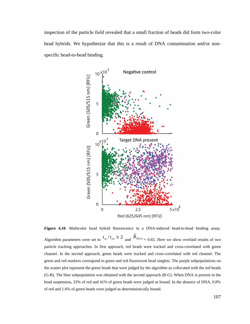
107

inspection of the particle field revealed that a small fraction of beads did form two-color

bead hybrids. We hypothesize that this is a result of DNA contamination and/or non-

specific bead-to-bead binding.

Figure 4.10. Multicolor bead hybrid fluorescence in a DNA-induced bead-to-bead binding assay.

Algorithm parameters were set to 2/ ≅chm tt and coIDR ,~

= 0.65. Here we show overlaid results of two

particle tracking approaches. In first approach, red beads were tracked and cross-correlated with green

channel. In the second approach, green beads were tracked and cross-correlated with red channel. The

green and red markers correspond to green and red fluorescent bead singlets. The purple subpopulations on

the scatter plot represent the green beads that were judged by the algorithm as collocated with the red beads

(G-R). The blue subpopulation was obtained with the second approach (R-G). When DNA is present in the

bead suspension, 33% of red and 41% of green beads were judged as bound. In the absence of DNA, 0.8%

of red and 1.6% of green beads were judged as deterministically bound.

108

5 Conclusions, contributions, and recommendations

In this chapter, we summarize the main conclusions and major achievements of the work

presented in this dissertation. We also present recommendations for future work,

including ideas for significant extensions of the current work. Sections 4.1 through 4.3

respectively describe the major conclusions, contributions, and recommendations of our

work on (1) bacterial RNA extraction and purification from whole human blood using

ITP, (2) temperature effects on electrophoresis and (3) particle tracking and multispectral

collocation method for particle-to-particle binding assays.

5.1 Summary of conclusions

5.1.1 Bacterial RNA Extraction and Purification from Whole Human Blood Using Isotachophoresis

1. Alkali-based lysing is well compatible with ITP extraction chemistry. ITP-based

extraction and purification was shown efficacious for 16S rRNA from

Pseudomonas Putida bacteria suspended in whole human blood.

2. The assay can be implemented with minimal manual steps and can automate the

extraction, preconcentration, and purification of nucleic acid in less than 5 min.

3. RNA is easily hydrolyzed at elevated temperature, and at either alkali or acidic

conditions. Further, its stability is significantly compromised by the abundance of

RNases in blood. We showed that a novel ITP and PCR compatible chemistry

109

which ensures RNA stability and recovery using the addition of DTT, a strong

reducing agent, and large amounts of polyA carrier RNA.

4. We showed that the extracted 16S rRNA was purified of PCR inhibitors and

compatible with RT-qPCR. We demonstrated a sensitivity of 0.03 bacteria per

nanoliter of blood, and hypothesize our sensitivity is currently limited by the

presence of RNA contaminants in our reagents.

5.1.2 Temperature Effects on Electrophoresis

1. Our approach of including the effects of (1) viscosity, (2) ionic strength, (3)

degree of ionization (pK), and (4) ion solvation effects on mobility, led to an

electrolyte solution simulation tool which predicts the effects of temperature on

ion mobility, solution pH, and solution conductivity.

2. We measured the temperature dependence of conductivity and pH in detail for ten

electrolyte solutions. For temperatures between 20°C and 70°C, our electrolyte

simulation tool was able to accurately predict conductivity and pH within 4% and

~ 0.2 pH units, respectively.

3. The model included a treatment of key phenomena, such that experimental

validation was possible across a wide range of buffers including Tris-HCl, and

enthanolamine-borate. In the case of Tris-HCl, we found that the non-viscosity

related temperature dependence is due to the change in the hydration shell of the

chloride ion. Whereas the temperature dependence of enthanolamine-borate

conductivity and pH is dominated by the change in the degree of ionization of its

constituent weak electrolyte ions.

110

4. The model predictions show and experiments confirm temperature sensitivity of

electrolyte solution pH, and the clear presence of non-viscosity related

temperature effects on conductivity.

5. For some electrolytes, the temperature induced reduction in degree of ionization

strongly compensates for decreases in water viscosity, resulting in moderate

conductivity increases (and even local maxima) with increasing temperature. For

other electrolyte solutions, viscosity remains the dominant source of temperature

dependence of conductivity, but pH can still vary significantly.

6. Walden’s rule alone can lead to large errors. For example, Walden’s rule yields

75% error for 20 mM ethanolamine and 20 mM boric acid solution, and 30%

error for 30 mM Tris and 30mM HEPES solution conductivities.

5.1.3 Particle Tracking and Multispectral Collocation Method for Cytometry-Like and Particle-to-Particle Binding Assays

1. A custom algorithm which identifies, and tracks particle parameters was shown

by simulations and experiments to capture cytometry-like data and particle

collocation data for thousands of particles, using a relatively simple experiment.

The data included size, intensity and collocation with other wavelengths.

2. Algorithm validation via Monte Carlo simulations of particle images at various

image SNR and particle densities demonstrated that the algorithm can be

relatively robust with just a few user-specified parameters. Analyses suggest that

the optimum algorithm performance is achieved for SNR > 5 and inter-particle

distance of LIP > 3 Lch. For particle-to-particle collocation we recommend

multiple realizations through monitoring times of tm > 2 tch.

111

3. The collocation algorithm and imaging technique was demonstrated as a method

for quantifying DNA target identification by flowing oligonucleotide

functionalized fluorescent bead populations in the presence of DNA targets to

induce bead-to-bead binding. The algorithm was able to identify thousands of

unique beads, over 1000 of which were monitored for 5 s or longer. Time-

resolved fluorescent intensity and collocation with other channels were obtained

and analyzed for detection of the target molecule. We found that in positive

control experiments, over 400 of each bead set (~40%) participated in a bead-

DNA-bead hybrid. In the negative control, the number of beads identified as

collocated with another color was roughly 1%.

4. Out method has capabilities beyond those offered by conventional flow cytometry

(FCM). For example, unlike FCM, our method obtains multiple realization of the

same particle, so we can monitor kinetic events (e.g.: time evolution of particle

intensity, size, or collocation) Furthermore, we do not require precise

hydrodynamic focusing, or significant particle/cell dilution (we can operate with

108 particles/mL).

5.2 Summary of major contributions

5.2.1 Bacterial RNA Extraction and Purification from Whole Human Blood Using Isotachophoresis

1. Development of ITP compatible lysing chemistry enabling RNA isolation from

ribonuclease- (RNase) rich samples such as biological fluids and cell-free

suspensions (e.g., whole blood).

112

2. Optimization of RNA extraction protocol to be performed entirely in aqueous

solution. Lysing chemistry is directly compatible with downstream transduction

methods, including but not limited to enzymatic- (reverse-transcription (RT),

polymerase chain reaction (PCR, ligation, etc.) and hybridization-based (e.g.,

RNA microarray chips) assays.

3. Integration and automation of RNA extraction protocol with ITP-based

purification, and on-chip RNA detection.

4. Extraction and purification of bacterial RNA from whole human blood.

Demonstration of compatibility with reverse transcription-quantitative polymerase

chain reaction (RT-qPCR).

5. Demonstration of clinically relevant sensitivity of 0.03 bacteria per nanoliter

blood using RT-qPCR.

5.2.2 Temperature Effects on Electrophoresis

1. Development of model capturing the important contributors to the effects of

temperature on the observable electrophoretic mobilities of small ions, and on

solution conductivity and pH. Model includes temperature effects on viscosity,

ionic strength corrections, degree of ionization (pK), and ion solvation.

Specifically, the model includes thermophysical data of the temperature

dependence of the water viscosity; the temperature dependence of the Onsager-

Fuoss model for finite ionic strength effects on mobility; the temperature

dependence of the extended Debye-Huckel theory for correction of ionic activity;

the Clarke-Glew generalized approach to predict the acid dissociation constant,

pK, from tabulated thermodynamic properties; and species-specific, empirically

113

evaluated correction terms for temperature-dependence of Stokes’ radii of 11

common small ions.

2. Development of free, open source MATLAB-based simulation tool named

Simulation of Temperature Effects on ElectroPhoresis (STEEP).

3. Experimental validation of STEEP using conductance and pH measurements

across a temperature variation of 25°C to 70°C for a set of electrolytes routinely

used in electrophoresis.

5.2.3 Particle Tracking and Multispectral Collocation Method for Cytometry-Like and Particle-to-Particle Binding Assays

1. Development of particle imaging, tracking and collocation (PITC) algorithm

applicable for analysis of either single images or time-resolved and spectrally-

separated images of the motion of randomly distributed particles.

2. Optimization and validation of PITC algorithm parameters using Monte Carlo

simulations. This study showed that our PITC algorithm is robust given sufficient

image SNR (SNR>5) even at high particle densities (108 /mL). For example, we

have shown that we can track thousands of particles, and collect time-resolved

multiparametric data in less than 5 min.

3. Demonstrated high throughput capability. For applications requiring a single

realization per particle, our method can produce particle size and multispectral

intensity data for roughly 100-200 particles per realization, where the frequency

of data capture is limited by CCD camera readout rates. With our setup (readout

time: 35 ms, exposure time: 5 s), this translates to 120,000-240,000 particle scans

per minute.

114

4. Experimental demonstration of the tracking and collocation method on

challenging image data, including flow of randomly distributed Brownian bead

populations which undergo bead-to-bead binding induced by hybridization to 16S

rRNA gene.

5.3 Recommendations for future work

5.3.1 Bacterial RNA Extraction and Purification from Whole Human Blood Using Isotachophoresis

1. In order to improve sensitivity, and ease of use, we can envision a disposable

plastic chip that can be discarded after each use, largely mitigating

decontamination and obviating surface re-conditioning procedures.

2. With the current channel design, we expect, at most, 2 orders of magnitude

improvement in sensitivity by addressing the presence of RNA contaminants in

our reagents. To achieve higher sensitivity, our method will likely require

redesign of chip geometry to achieve higher extraction efficiency and to

accommodate processing of larger sample volumes. We hypothesize that, given

sufficient sample capacity, our RNA extraction method can be made compatible

with DNA or RNA chips, perhaps without the need for nucleic acid amplification.

5.3.2 Temperature Effects on Electrophoresis

1. Modification of SPRESSO, a free, open-source MATLAB-based nonlinear

electrophoresis solver, to account for temperature effects could enable more

complex, and ad hoc separation optimizations which can accurately capture

electromigration dispersion and so-called system zones at elevated temperature.

115

2. To simulate the effect of externally imposed axial and radial temperature

gradients on electrophoretic separations and focusing, we recommend performing

temperature-dependent calculations at every grid point in the domain.

3. Further enhancement of the simulation capabilities can be achieved by iterative

computation of the Joule heating induced changes in conductivity and

corresponding changes in local temperature.

5.3.3 Particle Tracking and Multispectral Collocation Method for Cytometry-Like and Particle-to-Particle Binding Assays

1. The particle tracking phase of the algorithm (KC-PTV) can be further refined by

including other particle parameters in the χ2-test. For example, the accuracy of

particle matches can be improved by including particle shape, orientation (angle),

and complexity (intensity distribution), in addition to coordinates and size among

the χ2-test criteria.

2. While we have optimized and demonstrated this method for challenging image

data of particle-to-particle binding assays, we note that this method is equally

applicable for assays where particles are not expected to interact. For instance, our

method can be applied for rapid cell-based diagnostics (e.g., TB and malaria)168 or

for 2-4 color immunophenotyping assays.173

3. This method is particularly appealing as it lends itself to the efforts of cost

reduction for cell enumeration technologies (e.g., see Mandy et al.181 for

discussion of affordable CD4+ T-cell enumeration). One affordable option is to

sequentially trigger each wavelength of a four-color high power Thorlabs LED

source $5k (price includes driver and modulation input) and collect images at a

116

fixed time offset. Alternatively one can use an emission splitter devices (as we

have done so in this study) which can costs $8k (2-color Cairn Optosplit II image

splitter and cube) up to $19k (4-color Photometrics Quad-View 2 System).

4. We have demonstrated that we can detect the presence of nucleic acids indirectly

by monitoring bead-to-bead binding. We recommend exploring the limit of

detection of molecular biomarkers (proteins, RNA and DNA), and evaluating

weather this method can achieve a clinically relevant sensitivity required for

diagnostic purposes.

117

6 Bibliography

[1] Farrell, R.E., "RNA methodologies: A laboratory guide for isolation and

characterization". 4 ed. 2010, San Diego, CA: Academic Press, Inc.

[2] Wellinghausen, N., et al., "Diagnosis of bacteremia in whole-blood samples by

use of a commercial universal 16S rRNA gene-based PCR and sequence

analysis", Journal of clinical microbiology, 2009, 47 (9), 2759-2765.

[3] Zhang, Y., et al., "Detection of Streptococcus pneumoniae in whole blood by

PCR", Journal of clinical microbiology, 1995, 33 (3), 596-601.

[4] Marck, C. and H. Grosjean, "tRNomics: Analysis of tRNA genes from 50

genomes of Eukarya, Archaea, and Bacteria reveals anticodon-sparing strategies

and domain-specific features", Rna-a Publication of the Rna Society, 2002, 8 (10),

1189-1232.

[5] Alberts, B., et al., "Molecular biology of the cell 4th edition". 2002: Garland

Science, a Taylor & Francis Group.

[6] Satterfield, B.C., et al., "Microfluidic Purification and Preconcentration of mRNA

by Flow-Through Polymeric Monolith", Analytical Chemistry, 2007, 79 (16),

6230-6235.

[7] Lowery, A.J., et al., "MicroRNAs as Prognostic Indicators and Therapeutic

Targets: Potential Effect on Breast Cancer Management", Clinical Cancer

Research, 2008, 14 (2), 360-365.

118

[8] Dheda, K., et al., "Validation of housekeeping genes for normalizing RNA

expression in real-time PCR", Biotechniques, 2004, 37, 112-119.

[9] He, L. and G.J. Hannon, "MicroRNAs: small RNAs with a big role in gene

regulation", Nature Reviews Genetics, 2004, 5 (7), 522-531.

[10] Mueller, O., S. Lightfoot, and A. Schroder, "RNA Integrity Number (RIN)

Standardization of RNA Quality Control", Tech. Rep. 5989-1165EN, Agilent

Technologies, Application Note, 2004.

[11] Schroeder, A., et al., "The RIN: an RNA integrity number for assigning integrity

values to RNA measurements", BMC Molecular Biology, 2006, 7 (1), 3.

[12] Tsui, N.B.Y., E.K.O. Ng, and Y.M.D. Lo, "Stability of Endogenous and Added

RNA in Blood Specimens, Serum, and Plasma", Clinical Chemistry, 2002, 48

(10), 1647-1653.

[13] Cox, R., H.J. Gould, and K. Kanagalingam, "A study of the alkaline hydrolysis of

fractionated reticulocyte ribosomal ribonucleic acid and its relevance to secondary

structure", Biochemical Journal, 1968, 106 (3), 733.

[14] Lipkin, D., P.T. Talbert, and M. Cohn, "The Mechanism of the Alkaline

Hydrolysis of Ribonucleic Acids", Journal of the American Chemical Society,

1954, 76 (11), 2871-2872.

[15] Wang, H., R.A. Ach, and B. Curry, "Direct and sensitive miRNA profiling from

low-input total RNA", RNA, 2007, 13 (1), 151-159.

119

[16] Dunbar, S.A., "Applications of Luminex® xMAP™ technology for rapid, high-

throughput multiplexed nucleic acid detection", Clinica Chimica Acta, 2006, 363

(1–2), 71-82.

[17] Xu, R.N., et al., "Recent advances in high-throughput quantitative bioanalysis by

LC–MS/MS", Journal of Pharmaceutical and Biomedical Analysis, 2007, 44 (2),

342-355.

[18] Toner, M. and D. Irimia, "BLOOD-ON-A-CHIP", Annual Review of Biomedical

Engineering, 2005, 7 (1), 77-103.

[19] Johansson, M.A. and K.-E. Hellenäs, "Matrix effects in immunobiosensor

determination of clenbuterol in urine and serum", Analyst, 2004, 129 (5), 438-

442.

[20] Chambers, E., et al., "Systematic and comprehensive strategy for reducing matrix

effects in LC/MS/MS analyses", Journal of chromatography. B, Analytical

technologies in the biomedical and life sciences, 2007, 852 (1-2), 22-34.

[21] Chiu, M.L., et al., "Matrix Effects—A Challenge Toward Automation of

Molecular Analysis", JALA, 2010, 15 (3), 233-242.

[22] Lagally, E.T., et al., "Integrated Portable Genetic Analysis Microsystem for

Pathogen/Infectious Disease Detection", Analytical Chemistry, 2004, 76 (11),

3162-3170.

120

[23] Peytavi, R., et al., "Microfluidic Device for Rapid (<15 min) Automated

Microarray Hybridization", Clin Chem, 2005, 51 (10), 1836-1844.

[24] Grob, R.L., "Sample Preparation Techniques Used for Gas Chromatography",

Retrieved from http://www.restek.com/Technical-Resources/Technical-

Library/Editorial/editorial_A005.

[25] Mariella, R., "Sample preparation: the weak link in microfluidics-based

biodetection", Biomedical Microdevices, 2008, 10 (6), 777-784.

[26] Chomczynski, P. and N. Sacchi, "Single-step method of RNA isolation by acid

guanidinium thiocyanate-phenol-chloroform extraction", Analytical

Biochemistry, 1987, 162 (1), 156-159.

[27] Arthur, C.L. and J. Pawliszyn, "Solid phase microextraction with thermal

desorption using fused silica optical fibers", Analytical Chemistry, 1990, 62 (19),

2145-2148.

[28] Wen, J., et al., "Purification of Nucleic Acids in Microfluidic Devices",

Analytical Chemistry, 2008, 80 (17), 6472-6479.

[29] Uhlen, M., "Magnetic separation of DNA", Nature, 1989, 340 (6236), 733-734.

[30] Lee, J.-H., et al., "Comparisons of Three Automated Systems for Genomic DNA

Extraction in a Clinical Diagnostic Laboratory", Yonsei Med J, 2010, 51 (1), 104-

110.

121

[31] Breadmore, M.C., et al., "Microchip-Based Purification of DNA from Biological

Samples", Analytical Chemistry, 2003, 75 (8), 1880-1886.

[32] Legendre, L.A., et al., "A Simple, Valveless Microfluidic Sample Preparation

Device for Extraction and Amplification of DNA from Nanoliter-Volume

Samples", Analytical Chemistry, 2006, 78 (5), 1444-1451.

[33] Root, B.E., et al., "Purification of HIV RNA from Serum Using a Polymer

Capture Matrix in a Microfluidic Device", Analytical Chemistry, 2011, 83 (3),

982-988.

[34] Witek, M.A., et al., "96-Well Polycarbonate-Based Microfluidic Titer Plate for

High-Throughput Purification of DNA and RNA", Analytical Chemistry, 2008,

80 (9), 3483-3491.

[35] Bhattacharyya, A. and C.M. Klapperich, "Microfluidics-based extraction of viral

RNA from infected mammalian cells for disposable molecular diagnostics",

Sensors and Actuators B: Chemical, 2008, 129 (2), 693-698.

[36] Jiang, G. and D.J. Harrison, "mRNA isolation in a microfluidic device for

eventual integration of cDNA library construction", Analyst, 2000, 125 (12).

[37] Hong, J.W., et al., "A nanoliter-scale nucleic acid processor with parallel

architecture", Nat Biotech, 2004, 22 (4), 435-439.

[38] Hagan, K.A., et al., "Microchip-Based Solid-Phase Purification of RNA from

Biological Samples", Analytical Chemistry, 2008, 80 (22), 8453-8460.

122

[39] Hagan, K.A., et al., "Chitosan-Coated Silica as a Solid Phase for RNA

Purification in a Microfluidic Device", Analytical Chemistry, 2009, 81 (13),

5249-5256.

[40] Garcia-Schwarz, G., et al., "On-chip Isotachophoresis for Separation of Ions and

Purification of Nucleic Acids", J Vis Exp, 2012 (61), e3890.

[41] Jung, B., R. Bharadwaj, and J.G. Santiago, "On-Chip Millionfold Sample

Stacking Using Transient Isotachophoresis", Analytical Chemistry, 2006, 78 (7),

2319-2327.

[42] Khurana, T.K. and J.G. Santiago, "Sample Zone Dynamics in Peak Mode

Isotachophoresis", Analytical Chemistry, 2008, 80 (16), 6300-6307.

[43] Bercovici, M., et al., "Rapid hybridization of nucleic acids using

isotachophoresis", Proc. Natl. Acad. Sci., 2012, 109 (28), 11127-11132.

[44] Manual, W.E., "Worthington Biochemical Corp". Freehold, NJ. Vol. 43. 1972.

[45] "Reverse Transcriptase Enzymes", 2013; Available from:

http://www.invitrogen.com/site/us/en/home/Products-and-

Services/Applications/PCR/reverse-transcription/reverse-transcriptase-

enzymes.html.

[46] Wetmur, J.G. and J. Fresco, "DNA Probes: Applications of the Principles of

Nucleic Acid Hybridization", Critical Reviews in Biochemistry and Molecular

Biology, 1991, 26 (3-4), 227-259.

123

[47] Wetmur, J.G. and N. Davidson, "Kinetics of renaturation of DNA", Journal of

Molecular Biology, 1968, 31 (3), 349-370.

[48] Wetmur, J.G., "Hybridization and Renaturation Kinetics of Nucleic Acids",

Annual Review of Biophysics and Bioengineering, 1976, 5 (1), 337-361.

[49] Kestin, J., "Viscosity of Liquid Water in the Range—8 C to 150 C", J. Phys.

Chem. Ref. Data, 1978, 7 (3).

[50] Liu, S., et al., "Optimization of High-Speed DNA Sequencing on Microfabricated

Capillary Electrophoresis Channels", Analytical Chemistry, 1998, 71 (3), 566-

573.

[51] Liang, D. and B. Chu, "High speed separation of DNA fragments by capillary

electrophoresis in poly(ethylene oxide)-poly(propylene oxide)-poly(ethylene

oxide) triblock polymer", ELECTROPHORESIS, 1998, 19 (14), 2447-2453.

[52] Zhang, J., et al., "Use of Non-Cross-Linked Polyacrylamide for Four-Color DNA

Sequencing by Capillary Electrophoresis Separation of Fragments up to 640

Bases in Length in Two Hours", Analytical Chemistry, 1995, 67 (24), 4589-4593.

[53] Landers, J.P., "Handbook of capillary electrophoresis". 2 ed, ed. J.P. Landers.

2008, Boca Raton, FL: CRC Press, Taylor and Francis Group, LLC 27-28.

[54] Grushka, E., R.M. McCormick, and J.J. Kirkland, "Effect of temperature

gradients on the efficiency of capillary zone electrophoresis separations",

Analytical Chemistry, 1989, 61 (3), 241-246.

124

[55] Tang, G., et al., "Joule heating effect on electroosmotic flow and mass species

transport in a microcapillary", International Journal of Heat and Mass Transfer,

2004, 47 (2), 215-227.

[56] Petersen, N.J., et al., "Effect of Joule heating on efficiency and performance for

microchip-based and capillary-based electrophoretic separation systems: A closer

look", ELECTROPHORESIS, 2004, 25 (2), 253-269.

[57] Evenhuis, C.J., et al., "Temperature Profiles and Heat Dissipation in Capillary

Electrophoresis", Analytical Chemistry, 2006, 78 (8), 2684-2693.

[58] Xuan, X., "Joule heating in electrokinetic flow", ELECTROPHORESIS, 2007, 29

(1), 33-43.

[59] Gaš, B. and E. Kenndler, "Dispersive phenomena in electromigration separation

methods", ELECTROPHORESIS, 2000, 21 (18), 3888-3897.

[60] Štědrý, M., M. Jaroš, and B. Gaš, "Eigenmobilities in background electrolytes for

capillary zone electrophoresis: I. System eigenpeaks and resonance in systems

with strong electrolytes", Journal of Chromatography A, 2002, 960 (1–2), 187-

198.

[61] Štědrý, M., et al., "Eigenmobilities in background electrolytes for capillary zone

electrophoresis: III. Linear theory of electromigration", ELECTROPHORESIS,

2004, 25 (18-19), 3071-3079.

125

[62] Gaš, B. and E. Kenndler, "System zones in capillary zone electrophoresis",

ELECTROPHORESIS, 2004, 25 (23-24), 3901-3912.

[63] Gebauer, P., J.L. Beckers, and P. Boček, "Theory of system zones in capillary

zone electrophoresis", ELECTROPHORESIS, 2002, 23 (12), 1779-1785.

[64] Jaros, M., et al., "Optimization of background electrolytes for capillary

electrophoresis: II. Computer simulation and comparison with experiments",

ELECTROPHORESIS, 2002, 23 (16), 2667-2677.

[65] Hruška, V., M. Jaroš, and B. Gaš, "Simul 5 – Free dynamic simulator of

electrophoresis", ELECTROPHORESIS, 2006, 27 (5-6), 984-991.

[66] Bahga, S.S., M. Bercovici, and J.G. Santiago, "Ionic strength effects on

electrophoretic focusing and separations", ELECTROPHORESIS, 2010, 31 (5),

910-919.

[67] Bercovici, M., S.K. Lele, and J.G. Santiago, "Open source simulation tool for

electrophoretic stacking, focusing, and separation", Journal of Chromatography

A, 2009, 1216 (6), 1008-1018.

[68] Saiki, R.K., et al., "Primer-directed enzymatic amplification of DNA with a

thermostable DNA polymerase", Science, 1988, 239 (4839), 487-487.

[69] Pickett, M.A., et al., "The plasmids of Chlamydia trachomatis and Chlamydophila

pneumoniae (N16): accurate determination of copy number and the paradoxical

effect of plasmid-curing agents", Microbiology, 2005, 151 (3), 893-893.

126

[70] Apfalter, P., et al., "Comparison of a new quantitative ompA-based real-time PCR

TaqMan assay for detection of Chlamydia pneumoniae DNA in respiratory

specimens with four conventional PCR assays", Journal of clinical microbiology,

2003, 41 (2), 592-592.

[71] Weidmann, M., U. Meyer-Konig, and F.T. Hufert, "Rapid detection of herpes

simplex virus and varicella-zoster virus infections by real-time PCR", Journal of

clinical microbiology, 2003, 41 (4), 1565-1565.

[72] Al-Soud, W.A. and P. Rådström, "Purification and Characterization of PCR-

Inhibitory Components in Blood Cells", Journal of Clinical Microbiology, 2001,

39 (2), 485-493.

[73] Al-Soud, W.A. and P. Rådström, "Effects of amplification facilitators on

diagnostic PCR in the presence of blood, feces, and meat", Journal of Clinical

Microbiology, 2000, 38 (12), 4463-4470.

[74] Wagner, A., et al., "Surveys of Gene Families Using Polymerase Chain Reaction:

PCR Selection and PCR Drift", Systematic Biology, 1994, 43 (2), 250-261.

[75] Multer, G.L. and K.A. Boynton, "PCR bias in amplification of androgen receptor

alleles, a trinucleotide repeat marker used in clonality studies", Nucleic Acids

Research, 1995, 23 (8), 1411-1418.

[76] Markoulatos, P., N. Siafakas, and M. Moncany, "Multiplex polymerase chain

reaction: A practical approach", Journal of Clinical Laboratory Analysis, 2002, 16

(1), 47-51.

127

[77] Voelkerding, K.V., S.A. Dames, and J.D. Durtschi, "Next-generation sequencing:

from basic research to diagnostics", Clinical chemistry, 2009, 55 (4), 641-641.

[78] Ozsolak, F., et al., "Amplification-free digital gene expression profiling from

minute cell quantities", Nature methods, 2010, 7 (8), 619-621.

[79] Metzker, M.L., "Sequencing technologies—the next generation", Nature Reviews

Genetics, 2009, 11 (1), 31-46.

[80] Liao, J.C., et al., "Use of electrochemical DNA biosensors for rapid molecular

identification of uropathogens in clinical urine specimens", Journal of clinical

microbiology, 2006, 44 (2), 561-561.

[81] Xu, L., et al., "Giant magnetoresistive biochip for DNA detection and HPV

genotyping", Biosensors and Bioelectronics, 2008, 24 (1), 99-103.

[82] Heller, M.J., "DNA MICROARRAY TECHNOLOGY: Devices, Systems, and

Applications", Annual Review of Biomedical Engineering, 2002, 4 (1), 129-153.

[83] Templin, M.F., et al., "Protein microarray technology", Trends in Biotechnology,

2002, 20 (4), 160-166.

[84] Squires, T.M., R.J. Messinger, and S.R. Manalis, "Making it stick: convection,

reaction and diffusion in surface-based biosensors", Nature biotechnology, 2008,

26 (4), 417-426.

[85] Minichino, C., "FY07 Engineering Research and Technology Report", 2008,

Lawrence Livermore National Laboratory (LLNL), Livermore, CA.

128

[86] Nam, J.-M., S.I. Stoeva, and C.A. Mirkin, "Bio-Bar-Code-Based DNA Detection

with PCR-like Sensitivity", Journal of the American Chemical Society, 2004, 126

(19), 5932-5933.

[87] Leslie, D.C., et al., "New Detection Modality for Label-Free Quantification of

DNA in Biological Samples via Superparamagnetic Bead Aggregation", Journal

of the American Chemical Society, 2012, 134 (12), 5689-5696.

[88] Rogacs, A., Y. Qu, and J.G. Santiago, "Bacterial RNA Extraction and Purification

from Whole Human Blood Using Isotachophoresis", Analytical Chemistry, 2012,

84 (14), 5858-5863.

[89] Matsuda, K., et al., "Sensitive Quantitative Detection of Commensal Bacteria by

rRNA-Targeted Reverse Transcription-PCR", Applied and Environmental

Microbiology, 2007, 73 (1), 32-39.

[90] Fujimori, M., et al., "Efficacy of bacterial ribosomal RNA-targeted reverse

transcription-quantitative PCR for detecting neonatal sepsis: a case control study",

BMC pediatrics, 2010, 10 (1), 53.

[91] Arfvidsson, C. and K.G. Wahlund, "Time-minimized determination of ribosome

and tRNA levels in bacterial cells using flow field-flow fractionation", Analytical

Biochemistry, 2003, 313 (1), 76-85.

[92] Neidhardt, F.C., "Escherichia coli and Salmonella". Vol. 1. 1996: ASM Press

129

[93] Kim, J., et al., "Microfluidic sample preparation: cell lysis and nucleic acid

purification", Integrative Biology, 2009, 1 (10), 574-586.

[94] Markham, R. and J. Smith, "The structure of ribonucleic acids. 1. Cyclic

nucleotides produced by ribonuclease and by alkaline hydrolysis", Biochemical

Journal, 1952, 52 (4), 552.

[95] Mahalanabis, M., et al., "Cell lysis and DNA extraction of gram-positive and

gram-negative bacteria from whole blood in a disposable microfluidic chip", Lab

on a Chip, 2009, 9 (19), 2811-2817.

[96] Jung, B., Y. Zhu, and J.G. Santiago, "Detection of 100 aM Fluorophores Using a

High-Sensitivity On-Chip CE System and Transient Isotachophoresis", Analytical

Chemistry, 2006, 79 (1), 345-349.

[97] Bahga, S.S., et al., "High-sensitivity detection using isotachophoresis with

variable cross-section geometry", ELECTROPHORESIS, 2011, 32 (5), 563-572.

[98] Boček, P., "Analytical isotachophoresis", 1981, Springer Berlin / Heidelberg.

131-177.

[99] Schoch, R.B., M. Ronaghi, and J.G. Santiago, "Rapid and selective extraction,

isolation, preconcentration, and quantitation of small RNAs from cell lysate using

on-chip isotachophoresis", Lab on a Chip, 2009, 9 (15), 2145-2152.

[100] Persat, A., et al., "Quantification of Global MicroRNA Abundance by Selective

Isotachophoresis", Analytical Chemistry, 2010, 82 (23), 9631-9635.

130

[101] Persat, A. and J.G. Santiago, "MicroRNA Profiling by Simultaneous Selective

Isotachophoresis and Hybridization with Molecular Beacons", Analytical

Chemistry, 2011, 83 (6), 2310-2316.

[102] Persat, A., L.A. Marshall, and J.G. Santiago, "Purification of Nucleic Acids from

Whole Blood Using Isotachophoresis", Analytical Chemistry, 2009, 81 (22),

9507-9511.

[103] Marshall, L.A., C.M. Han, and J.G. Santiago, "Extraction of DNA from Malaria-

Infected Erythrocytes Using Isotachophoresis", Analytical Chemistry, 2011, 83

(24), 9715-9718.

[104] Bercovici, M., et al., "Rapid Detection of Urinary Tract Infections Using

Isotachophoresis and Molecular Beacons", Analytical Chemistry, 2011, 83 (11),

4110-4117.

[105] Heptinstall, J., "Total RNA Isolation from Bacteria:The Nucleic Acid Protocols

Handbook", R. Rapley, Editor, 2000, Humana Press. 47-52.

[106] Bimboim, H. and J. Doly, "A rapid alkaline extraction procedure for screening

recombinant plasmid DNA", Nucleic acids research, 1979, 7 (6), 1513-1523.

[107] Freitas, S., et al., "On the stability of plasmid DNA vectors during cell culture and

purification", Molecular Biotechnology, 2007, 36 (2), 151-158.

[108] Florence, T.M., "Degradation of protein disulphide bonds in dilute alkali",

Biochemical Journal, 1980, 189 (3), 507.

131

[109] Lu, B.-Y. and J.-Y. Chang, "Rapid and irreversible reduction of protein disulfide

bonds", Analytical Biochemistry, 2010, 405 (1), 67-72.

[110] Chomczynski, P., "Solubilzation in formamide protects RNA from degradation",

Nucleic Acids Research, 1992, 20 (14), 3791-3792.

[111] Strauss Jr, J.H. and R.L. Sinsheimer, "Initial kinetics of degradation of MS2

ribonucleic acid by ribonuclease, heat and alkali and the presence of

configurational restraints in this ribonucleic acid", Journal of Molecular Biology,

1968, 34 (3), 453-465.

[112] Winslow, S.G. and P.A. Henkart, "Polyinosinlc acid as a carrier in the microscale

purification of total RNA", Nucleic Acids Research, 1991, 19 (12), 3251-3253.

[113] Gallagher, M.L., W.F. Burke Jr, and K. Orzech, "Carrier RNA enhancement of

recovery of DNA from dilute solutions", Biochemical and Biophysical Research

Communications, 1987, 144 (1), 271-276.

[114] Rio, D.C., et al., "Ethanol Precipitation of RNA and the Use of Carriers", Cold

Spring Harbor Protocols, 2010, 2010 (6).

[115] Shaw, K.J., et al., "The use of carrier RNA to enhance DNA extraction from

microfluidic-based silica monoliths", Analytica Chimica Acta, 2009, 652 (1–2),

231-233.

[116] Doherty, E.A.S., et al., "Microchannel wall coatings for protein separations by

capillary and chip electrophoresis", ELECTROPHORESIS, 2003, 24 (1-2), 34-54.

132

[117] McCormick, R.M., "Capillary zone electrophoretic separation of peptides and

proteins using low pH buffers in modified silica capillaries", Analytical

Chemistry, 1988, 60 (21), 2322-2328.

[118] Darton, T., et al., "Severity of Meningococcal Disease Associated with Genomic

Bacterial Load", Clinical Infectious Diseases, 2009, 48 (5), 587-594.

[119] Hackett, S.J., et al., "Meningococcal bacterial DNA load at presentation correlates

with disease severity", Archives of Disease in Childhood, 2002, 86 (1), 44-46.

[120] Rogacs, A. and J.G. Santiago, "Temperature Effects on Electrophoresis",

Analytical Chemistry, 2013, 85 (10), 5103-5113.

[121] Kelly, L. and R.J. Nelson, "Capillary Zone Electrophoresis of Organic Acids and

Anions", Journal of Liquid Chromatography, 1993, 16 (9-10), 2103-2112.

[122] Smith, S.C. and M.G. Khaledi, "Optimization of pH for the separation of organic

acids in capillary zone electrophoresis", Analytical Chemistry, 1993, 65 (3), 193-

198.

[123] Lin, C.-E., C.-C. Chang, and W.-C. Lin, "Migration behavior and separation of

sulfonamides in capillary zone electrophoresis III. Citrate buffer as a background

electrolyte", Journal of Chromatography A, 1997, 768 (1), 105-112.

[124] Rasmussen, H.T. and H.M. McNair, "Influence of buffer concentration, capillary

internal diameter and forced convection on resolution in capillary zone

electrophoresis", Journal of Chromatography A, 1990, 516 (1), 223-231.

133

[125] Hoffstetter-Kuhn, S., et al., "Influence of borate complexation on the

electrophoretic behavior of carbohydrates in capillary electrophoresis", Analytical

Chemistry, 1991, 63 (15), 1541-1547.

[126] Whang, C.W. and E.S. Yeung, "Temperature programming in capillary zone

electrophoresis", Analytical Chemistry, 1992, 64 (5), 502-506.

[127] Chang, H.-T. and E.S. Yeung, "Voltage programming in capillary zone

electrophoresis", Journal of Chromatography A, 1993, 632 (1–2), 149-155.

[128] Nübel, U., et al., "Sequence heterogeneities of genes encoding 16S rRNAs in

Paenibacillus polymyxa detected by temperature gradient gel electrophoresis",

Journal of Bacteriology, 1996, 178 (19), 5636-43.

[129] Rush, R.S., A.S. Cohen, and B.L. Karger, "Influence of column temperature on

the electrophoretic behavior of myoglobin and .alpha.-lactalbumin in high-

performance capillary electrophoresis", Analytical Chemistry, 1991, 63 (14),

1346-1350.

[130] Rochu, D., G. Ducret, and P. Masson, "Measuring conformational stability of

proteins using an optimized temperature-controlled capillary electrophoresis

approach", Journal of Chromatography A, 1999, 838 (1–2), 157-165.

[131] Ross, D. and L.E. Locascio, "Microfluidic Temperature Gradient Focusing",

Analytical Chemistry, 2002, 74 (11), 2556-2564.

134

[132] Shackman, J.G., et al., "Quantitative temperature gradient focusing performed

using background electrolytes at various pH values", ELECTROPHORESIS,

2006, 27 (17), 3420-3427.

[133] Ghosal, S. and Z. Chen, "Nonlinear Waves in Capillary Electrophoresis", Bulletin

of Mathematical Biology, 2010, 72 (8), 2047-2066.

[134] Nightingale, E.R., "Phenomenological Theory of Ion Solvation. Effective Radii of

Hydrated Ions", The Journal of Physical Chemistry, 1959, 63 (9), 1381-1387.

[135] Evenhuis, C.J., et al., "Reliable electrophoretic mobilities free from Joule heating

effects using CE", ELECTROPHORESIS, 2007, 28 (20), 3759-3766.

[136] Okamoto, H., et al., "Theory and computer programs for calculating solution pH,

buffer formula, and buffer capacity for multiple component system at a given

ionic strength and temperature", Pharmaceutical research, 1997, 14 (3), 299-302.

[137] Anderko, A. and M.M. Lencka, "Computation of electrical conductivity of

multicomponent aqueous systems in wide concentration and temperature ranges",

Industrial & engineering chemistry research, 1997, 36 (5), 1932-1943.

[138] Clancy, M.J., "The formulation of buffers and media for enzyme histochemistry",

The Histochemical Journal, 1987, 19 (1), 27-34.

[139] Beynon, R.J. and J.S. Easterby, "Buffer solutions". 1996: IRL Press at Oxford

University Press Oxford, UK.

135

[140] Fukada, H. and K. Takahashi, "Enthalpy and heat capacity changes for the proton

dissociation of various buffer components in 0.1 M potassium chloride", Proteins:

Structure, Function, and Bioinformatics, 1998, 33 (2), 159-166.

[141] Wang, C.-K. and H.-K. Tsao, "Temperature-Insensitive Electrokinetic Behavior

in Capillary Zone Electrophoresis", The Journal of Physical Chemistry B, 2004,

108 (45), 17685-17693.

[142] Reijenga, J.C., L.G. Gagliardi, and E. Kenndler, "Temperature dependence of

acidity constants, a tool to affect separation selectivity in capillary

electrophoresis", Journal of Chromatography A, 2007, 1155 (2), 142-145.

[143] Mandaji, M., et al., "Sample stacking in CZE using dynamic thermal junctions I.

Analytes with low dpKa/dT crossing a single thermally induced pH junction in a

BGE with high dpH/dT", ELECTROPHORESIS, 2009, 30 (9), 1501-1509.

[144] Milanova, D., et al., "Electrophoretic mobility measurements of fluorescent dyes

using on-chip capillary electrophoresis", ELECTROPHORESIS, 2011, 32 (22),

3286-3294.

[145] Diekmann, S., "Temperature and salt dependence of the gel migration anomaly of

curved DNA fragments", Nucleic Acids Research, 1987, 15 (1), 247-265.

[146] Kan, C.W. and A.E. Barron, "A DNA sieving matrix with thermally tunable mesh

size", ELECTROPHORESIS, 2003, 24 (1-2), 55-62.

136

[147] Evenhuis, C.J., et al., "Variation of zeta-potential with temperature in fused-silica

capillaries used for capillary electrophoresis", ELECTROPHORESIS, 2006, 27

(3), 672-676.

[148] Onsager, L. and R.M. Fuoss, "Irreversible Processes in Electrolytes. Diffusion,

Conductance and Viscous Flow in Arbitrary Mixtures of Strong Electrolytes",

The Journal of Physical Chemistry, 1931, 36 (11), 2689-2778.

[149] Grenthe, I. and H. Wanner, "TDB-2 Guidelines for the Extrapolation to Zero

Ionic Strength; minor revisions by Osthols", 2000, Erik.

[150] Debye, P. and E. Huckel, "The interionic attraction theory of deviations from

ideal behavior in solution", Z. Phys, 1923, 24, 185.

[151] Clarke, E.C.W. and D.N. Glew, "Evaluation of thermodynamic functions from

equilibrium constants", Transactions of the Faraday Society, 1966, 62 (0), 539-

547.

[152] Goldberg, R.N., N. Kishore, and R.M. Lennen, "Thermodynamic quantities for

the ionization reactions of buffers", Journal of Physical and Chemical Reference

Data, 2002, 31 (2), 231-370.

[153] Walden, P., H. Ulich, and G. Busch, "Leitfähigkeitsmessungen in aceton 1", Z.

Phys. Chem, 1926, 123, 429.

137

[154] Sadek, H., "Walden product, Stokes' law and water stucture: A critical review",

Journal of Electroanalytical Chemistry and Interfacial Electrochemistry, 1983,

144 (1–2), 11-32.

[155] Fernandez-Prini, R. and G. Atkinson, "Examination of the Zwanzig theory of

dielectric friction. II", The Journal of Physical Chemistry, 1971, 75 (2), 239-244.

[156] Jenkins, H.D.B. and Y. Marcus, "Viscosity B-Coefficients of Ions in Solution",

Chemical Reviews, 1995, 95 (8), 2695-2724.

[157] Porras, S.P., M.-L. Riekkola, and E. Kenndler, "The principles of migration and

dispersion in capillary zone electrophoresis in nonaqueous solvents",

ELECTROPHORESIS, 2003, 24 (10), 1485-1498.

[158] Robinson, R.A. and R.H. Stokes, "Electrolyte solutions". 2nd Revised ed. 2002,

New York: Dover Publications.

[159] Persat, A., M.E. Suss, and J.G. Santiago, "Basic principles of electrolyte

chemistry for microfluidic electrokinetics. Part II: Coupling between ion mobility,

electrolysis, and acid-base equilibria", Lab on a Chip, 2009, 9 (17), 2454-2469.

[160] Persat, A., R.D. Chambers, and J.G. Santiago, "Basic principles of electrolyte

chemistry for microfluidic electrokinetics. Part I: Acid–base equilibria and pH

buffers", Lab on a Chip, 2009, 9 (17), 2437-2453.

[161] Christensen, J.J., L.D. Hansen, and R.M. Izatt, "Handbook of proton ionization

heats and related thermodynamic quantities". 1976: Wiley New York.

138

[162] Wright, M.R., "An introduction to aqueous electrolyte solutions". 2007: Wiley.

[163] Lewis, G.N., Randall, M., Pitzer, K. S., Brewer, L., "Thermodynamics". 2 ed.

1961, New York: McGraw-Hill.

[164] Grenthe, I. and A. Plyasunov, "On the use of semiempirical electrolyte theories

for the modeling of solution chemical data", Pure and applied chemistry, 1997, 69

(5), 951-958.

[165] Olofsson, G. and L. Hepler, "Thermodynamics of ionization of water over wide

ranges of temperature and pressure", Journal of Solution Chemistry, 1975, 4 (2),

127-143.

[166] Hirokawa, T., M. Nishino, and Y. Kiso, "Isotachophoretic determination of

mobility and pKa by means of computer simulation: II. Evaluation of mo and pKa

of 65 anions", Journal of Chromatography A, 1982, 252, 49-65.

[167] Michov, B.M., "Specifying the equilibrium constants in Tris-borate buffers",

ELECTROPHORESIS, 1986, 7 (3), 150-151.

[168] Shapiro, H.M. and N.G. Perlmutter, "Killer applications: Toward affordable rapid

cell-based diagnostics for malaria and tuberculosis", Cytometry Part B: Clinical

Cytometry, 2008, 74 (S1), S152-S164.

[169] Tárnok, A. and A.O. Gerstner, "Clinical applications of laser scanning

cytometry", Cytometry, 2002, 50 (3), 133-143.

139

[170] Wilson, R., A.R. Cossins, and D.G. Spiller, "Encoded Microcarriers For High-

Throughput Multiplexed Detection", Angewandte Chemie International Edition,

2006, 45 (37), 6104-6117.

[171] Ortiz, M.E. and D. Endy, "Engineered cell-cell communication via DNA

messaging", Journal of biological engineering, 2012, 6 (1), 1-12.

[172] Leslie, D.C., et al., "New Detection Modality for Label-Free Quantification of

DNA in Biological Samples via Superparamagnetic Bead Aggregation", Journal

of the American Chemical Society, 2012, 134 (12), 5689-5696.

[173] De Rosa, S.C., J.M. Brenchley, and M. Roederer, "Beyond six colors: a new era

in flow cytometry", Nature medicine, 2003, 9 (1), 112-117.

[174] Lenz, D., et al., "Six and more color immunophenotyping on the slide by laser

scanning cytometry (LSC)", in Biomedical Optics 2003, 2003, International

Society for Optics and Photonics.

[175] Shapiro, H.M., "Practical flow cytometry". 2005: Wiley. com.

[176] Kamentsky, L.A. and L.D. Kamentsky, "Microscope-based multiparameter laser

scanning cytometer yielding data comparable to flow cytometry data", Cytometry,

1991, 12 (5), 381-387.

[177] Perfetto, S.P., P.K. Chattopadhyay, and M. Roederer, "Seventeen-colour flow

cytometry: unravelling the immune system", Nature Reviews Immunology, 2004,

4 (8), 648-655.

140

[178] Quirke, P. and J. Dyson, "Flow cytometry: methodology and applications in

pathology", The Journal of pathology, 1986, 149 (2), 79-87.

[179] Brown, M. and C. Wittwer, "Flow cytometry: principles and clinical applications

in hematology", Clinical chemistry, 2000, 46 (8), 1221-1229.

[180] Darzynkiewicz, Z., et al., "Laser-scanning cytometry: a new instrumentation with

many applications", Experimental cell research, 1999, 249 (1), 1-12.

[181] Mandy, F., et al., "Affordable CD4 T-cell enumeration for resource-limited

regions: A status report for 2008", Cytometry Part B: Clinical Cytometry, 2008,

74 (S1), S27-S39.

[182] Kinosita, K., et al., "Dual-view microscopy with a single camera: real-time

imaging of molecular orientations and calcium", The Journal of Cell Biology,

1991, 115 (1), 67-73.

[183] Chandrasekhar, S., "Stochastic problems in physics and astronomy", Reviews of

modern physics, 1943, 15 (1), 1.

[184] Einstein, A., "On the movement of small particles suspended in stationary liquids

required by the molecular-kinetic theory of heat", Annalen der Physik, 1905, 17

(549-560), 16.

[185] Meinhart, C., S. Wereley, and J. Santiago, "PIV measurements of a microchannel

flow", Experiments in Fluids, 1999, 27 (5), 414-419.

141

[186] Santiago, J.G., et al., "A particle image velocimetry system for microfluidics",

Experiments in Fluids, 1998, 25 (4), 316-319.

[187] Meinhart, C.D., S.T. Wereley, and J.G. Santiago, "PIV measurements of a

microchannel flow", Experiments in Fluids, 1999, 27 (5), 414-419.

[188] Wereley, S.T. and C.D. Meinhart, "Recent Advances in Micro-Particle Image

Velocimetry", Annual Review of Fluid Mechanics, 2010, 42 (1), 557-576.

[189] Adrian, R.J. and J. Westerweel, "Particle image velocimetry". Vol. 30. 2010:

Cambridge University Press.

[190] Raffel, M., et al., "Particle Image Velocimetry–A Pratical Guide". 2 ed. Particle

image velocimetry: a pratical guide. 2007, Heidelberg: Springer Press.

[191] Meinhart, C.D., S.T. Wereley, and J.G. Santiago, "A PIV algorithm for estimating

time-averaged velocity fields", Journal of Fluids Engineering, 2000, 122 (2), 285-

289.

[192] Takehara, K. and G.T. Etoh, "A study on particle identification in PTV particle

mask correlation method", Journal of Visualization, 1999, 1 (3), 313-323.

[193] Takehara, K., R. Adrian, and T. Etoh, "A new Super-Resolution method by using

the KC method", Journal of the Visualization Society of Japan, 1999, 19 (Suppl

1), 319-322.

[194] Takehara, K., et al., "A Kalman tracker for super-resolution PIV", Experiments in

Fluids, 2000, 29 (1), S034-S041.

142

[195] Devasenathipathy, S., J.G. Santiago, and K. Takehara, "Particle Tracking

Techniques for Electrokinetic Microchannel Flows", Analytical Chemistry, 2002,

74 (15), 3704-3713.

[196] Devasenathipathy, S., et al., "Particle imaging techniques for microfabricated

fluidic systems", Experiments in Fluids, 2003, 34 (4), 504-514.

143

7 Appendix A. ITP compatible lysis methods

Contents of this Appendix are under preparation for publication by Anita Rogacs,

Lewis A. Marshall, and Juan G. Santiago in the Journal of Chromatography A. They are

reproduced here with modifications.

KEY CONSIDERATIONS

Lysis protocols for DNA and RNA extractions should effectively disrupt cells or

tissues, denature proteins and nucleoprotein complexes, and inactivate endogenous

nucleases (e.g: DNase and RNase). For organisms that have cell walls in addition to a

cell membrane, the use of additional enzymes may be required for complete cell

disruption. For example, the cell membrane of gram-positive bacteria consists of many

layers or peptidoglycan (polymer consisting of sugars and amino acids), which are

notoriously difficult to lyse. The addition of lysozyme has been shown to disrupt the

bacterial cell walls very effectively.1 Similarly, the cell walls of yeast contain chitin and

other polysaccharides2 and require enzymatic digestion using zymolase or lyticase.3

Lysis methods compatible with ITP can be categorized into three major groups:

thermal, electrical, and chemical (including enzymatic) lysis. The thermal and electrical

approaches are often attractive, as they do not introduce PCR inhibiting species which

can co-focus with nucleic acids during ITP, nor do they alter ITP dynamics by changing

the solution pH or conductivity. However, chemical approaches are very convenient as

they can often be performed at room temperature with only addition of chemicals to the

sample (requiring no special equipment). We here focus mostly on off-chip lysing

144

methods performed prior to loading samples into the chip, but mention several on-chip

lysing methods.

DETERGENTS

Most mammalian and cultured cells lyse in presence of detergents. Ionic

detergents such as sodium dodecyl sulfate (SDS) can also denature proteins by binding to

charged side chains and causing local changes in protein conformation. ITP can be made

compatible with the anionic SDS (unpublished results), but the use of SDS is often

restrictive as it sets a minimum value on the trailing ion effective mobility (SDS has a

mobility of about 23 cm2/V/s)4. To keep denatured proteins in solution, and prevent their

aggregation, we recommend the addition of mild non-ionic detergents such Triton X-100

or Tween 20 to the lysis buffer (usually added at roughly the critical micelle

concentration). Non-ionic detergents are well compatible with ITP as they do not migrate

under electric field. Also, non-ionic surfactants are compatible with many downstream

assays including PCR (e.g.: Triton X-100 is a PCR adjunct below 10% w/v, which is

~103 times the CMC concentration).5

DENATURANTS

The denaturing step disrupts nucleoprotein complexes (e.g., disrupts chromatin

and releases chromosomal DNA from histone) by unfolding proteins. Examples of

chaotropic denaturing reagents include sodium tricholoroacetate, sodium perchlorate,

sodium thiocynate, urea, guanadinum thiocynate and guanadinium hydrochloride.6

Chaotropic-based protein denaturation requires the presence of these reagent at high

concentrations (6 M-10 M).7 These species strongly inhibit PCR, and with the exception

145

of urea, they contain fast anions that can co-focus with NA and even form a plateau zone

between LE and TE. The high concentrations of these ions in the lysate require

prohibitively long purification times for ITP-based extraction of NA (up to 10 h,

unpublished results). Also important, anionic chaotrope species can co-purify with the

NA. For applications which have strict requirements of chaotropic-based denaturation,

we recommend the use of urea. Urea is a non-ionic reagent, so it does not interfere with

ITP dynamics and stays behind (in the initial TE zone) during the purification process.

Our group has demonstrated urea compatibility with ITP at high concentrations.8

NUCLEASE INACTIVATION

Nuclease inactivation: Effective inactivation of endogenous nucleases (DNase and

RNase enzymes) is a key early step in the extraction process. DNases can usually be

inactivated by use chelating agents (e.g., ethylenediamine-tetraacetic acid, EDTA),9

which sequester magnesium ions that are essential for nuclease function. EDTA is a fast,

tetravalent anionic species, and as a result, in many ITP separation chemistries, EDTA

will overspeed DNA and RNA and the leading electrolyte (chloride). EDTA also inhibits

PCR at concentrations above 0.1 mM.5 One approach to purifying nucleic acid from

EDTA may be to initiate ITP into a waste well, and subsequently switch the ITP anode

into a separate extraction well. An alternative to EDTA for DNAse activation is to

increase temperature (>65 °C) or perform proteinase K digestion at 56 °C. Proteinase K is

a PCR inhibitor, but can be excluded easily by working with pH below about 8.5.10

Inactivation of ribonuclease (Rnase) is more challenging due to its highly resilient

nature and fast catalytic action on RNA. As one salient example, without adequate RNase

146

control, free RNA is non-amplifiable after 15 s of incubation in plasma or serum.11

Neither EDTA nor heat will inactivate RNase permanently.12,13 Other RNase inhibiting

agents are therefore required in RNA extraction protocols. RNase inhibitors include

ribonucleoside-vanadyl complex14 and RNasin,15 as well as other commercially available

proprietary reagents (e.g., RNAsecure sold by Ambion, or RNase Out sold by

Invitrogen). The ribonucleoside- vanadyl complex will also inhibit downstream reactions

such as in vitro translation and reverse transcription, so we do not recommended it.

Addition of reducing agents such as dithiothreitol (DTT) (pKa = 8.3 and 9.5) or 2

beta- mercaptoethanol (2B-ME) (pKa = 9.64) can enhance denaturation of disulfide bond

containing proteins and thereby also aid in ribonuclease inactivation.16 (Rnase activity

requires intact disulfide bonds.) However, because they are anions in their active state,

they can each co-focus with the NA during ITP. This co-focusing can be avoided by

choosing a suitably high mobility trailing ion, or by diluting the extracted RNA

suspension to contain no more than 10 mM DTT. Below this concentration, DTT is a

PCR adjunct. See detailed discussion on DTT-based RNase inactivation method in

Chapter 2.

Chomazinsky and Sacchi,17 showed that RNA solubilized in pure formamide

resist Rnase induced degradation. In practice, formamide is often added to aqueous

hybridization buffers to modify the melting temperature of RNA or DNA duplexes. One

may also be tempted to add formamide to lysing buffers to inactivate the Rnase enzymes.

However, we emphasize here that the RNase inhibition is only effective if solubilization

occurs in pure, deionized formamide. In fact, formamide should never be used as an

additive in an aqueous lysing or hybridization reaction when Rnase is believed to be

147

present. Our own observations suggest that, when mixed with water, formamide promotes

RNA degradation even at extremely high RNA concentrations (see Fig. A.1) Others have

also reported enhanced Rnase activity in the presence of aqueous formamide.18

To study the effect of RNA degradation, we recommend performing size-based

separation of RNA. Agilent's 2100 Bioanalyzer uses a lab on a chip approach to perform

capillary electrophoresis of fluorescently labeled RNA to determine both RNA

concentration and integrity. The on-chip RNA analysis is based on traditional gel

electrophoresis principles that enable RNA separation based on size. The RNA

electropherograms provides a detailed visual assessment of the quality of the RNA

sample. As degradation proceeds (Fig. A.1), there is a decrease in the 18S to 28S

ribosomal band ratio and an increase in the baseline signal between the two ribosomal

peaks and the lower marker.

The RNA Integrity Number (RIN), was developed by Agilent to remove

individual interpretation in RNA quality control and allow classification of RNA

integrity. Their software computes the RIN by accounting for the entire electrophoretic

trace,19 and assigns a RIN based on a numbering system from 1 to 10, with 1 being the

most degraded profile and 10 being the most intact. In Fig. A.1. we show various levels

of RNA degradation induced by blood and aqueous formamide.

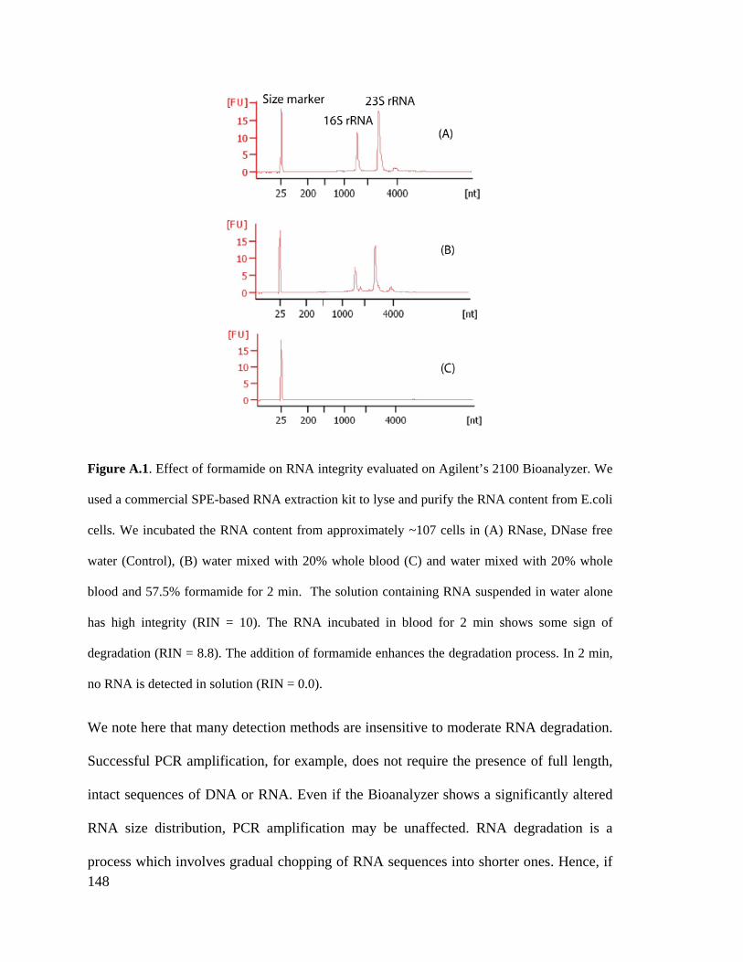
148

Figure A.1. Effect of formamide on RNA integrity evaluated on Agilent’s 2100 Bioanalyzer. We

used a commercial SPE-based RNA extraction kit to lyse and purify the RNA content from E.coli

cells. We incubated the RNA content from approximately ~107 cells in (A) RNase, DNase free

water (Control), (B) water mixed with 20% whole blood (C) and water mixed with 20% whole

blood and 57.5% formamide for 2 min. The solution containing RNA suspended in water alone

has high integrity (RIN = 10). The RNA incubated in blood for 2 min shows some sign of

degradation (RIN = 8.8). The addition of formamide enhances the degradation process. In 2 min,

no RNA is detected in solution (RIN = 0.0).

We note here that many detection methods are insensitive to moderate RNA degradation.

Successful PCR amplification, for example, does not require the presence of full length,

intact sequences of DNA or RNA. Even if the Bioanalyzer shows a significantly altered

RNA size distribution, PCR amplification may be unaffected. RNA degradation is a

process which involves gradual chopping of RNA sequences into shorter ones. Hence, if

149

> 50% of the sequence region bounded by the PCR probes remains intact during RNA

sample preparation, the amplification may remain unaffected by the degradation. Note,

that these regions are typically fairly short (~100 nt). In the study presented in Chapter 2,

we analyzed RNA integrity using Bioanalyzer, but we have also performed RT-PCR to

determine the upper tolerance for RNA degradation. In the study of Chapter 2, RNA

degradation which produced less than one cycle increase in the amplification threshold

cycle was deemed acceptable.

REFERENCES

[1] Liao, J.C., et al., "Use of electrochemical DNA biosensors for rapid molecular

identification of uropathogens in clinical urine specimens", Journal of Clinical

Microbiology, 2006, 44 (2), 561-570.

[2] Hudler, G.W., "Magical mushrooms, mischievous molds". 1998: Princeton

University Press.

[3] Salazar, O. and J. Asenjo, "Enzymatic lysis of microbial cells", Biotechnology

Letters, 2007, 29 (7), 985-994.

[4] Carchon, H. and E. Eggermont, "Isotachophoretic determination of a relative

apparent mobility as an estimate of the electrophoretic mobility of ions", Electrophoresis,

1982, 3 (5), 263-274.

[5] Kreader, C.A., "Relief of amplification inhibition in PCR with bovine serum

albumin or T4 gene 32 protein", Applied and Environmental Microbiology, 1996, 62 (3),

1102-1106.

150

[6] Hatefi, Y. and W.G. Hanstein, "Solubilization of Particulate Proteins and

Nonelectrolytes by Chaotropic Agents", Proceedings of the National Academy of

Sciences of the United States of America, 1969, 62 (4), 1129-1136.

[7] Greene, R.F. and C.N. Pace, "Urea and guanidine hydrochloride denaturation of

ribonuclease, lysozyme, α-chymotrypsin, and β-lactoglobulin", Journal of Biological

Chemistry, 1974, 249 (17), 5388-5393.

[8] Persat, A., et al., "Quantification of Global MicroRNA Abundance by Selective

Isotachophoresis", Analytical Chemistry, 2010, 82 (23), 9631-9635.

[9] Adams, R.L.P., J.T. Knowler, and D.P. Leader, "The biochemistry of the nucleic

acids". 1992: Chapman and Hall.

[10] Persat, A., L.A. Marshall, and J.G. Santiago, "Purification of Nucleic Acids from

Whole Blood Using Isotachophoresis", Analytical Chemistry, 2009, 81 (22), 9507-9511.

[11] Tsui, N.B.Y., E.K.O. Ng, and Y.M.D. Lo, "Stability of Endogenous and Added

RNA in Blood Specimens, Serum, and Plasma", Clinical Chemistry, 2002, 48 (10), 1647-

1653.

[12] Farrell, R.E., "RNA methodologies: A laboratory guide for isolation and

characterization". 4 ed. 2010, San Diego, CA: Academic Press, Inc.

[13] Steward, G.F. and A.I. Culley, "Extraction and purification of nucleic acids from

viruses", Manual of Aquatic Viral Ecology, 2010, 154-165.

151

[14] Berger, S.L. and C.S. Birkenmeier, "Inhibition of intractable, nucleases with

ribonucleoside-vanadyl complexes: isolation of messenger ribonucleic acid from resting

lymphocytes", Biochemistry, 1979, 18 (23), 5143-5149.

[15] Blackburn, P., G. Wilson, and S. Moore, "Ribonuclease inhibitor from human

placenta. Purification and properties", Journal of Biological Chemistry, 1977, 252 (16),

5904-5910.

[16] Lu, B.-Y. and J.-Y. Chang, "Rapid and irreversible reduction of protein disulfide

bonds", Analytical Biochemistry, 2010, 405 (1), 67-72.

[17] Chomczynski, P., "Solubilization in formamide protects RNA from degradation",

Nucleic Acids Research, 1992, 20 (14), 3791-3792.

[18] Strauss Jr, J.H. and R.L. Sinsheimer, "Initial kinetics of degradation of MS2

ribonucleic acid by ribonuclease, heat and alkali and the presence of configurational

restraints in this ribonucleic acid", Journal of Molecular Biology, 1968, 34 (3), 453-465.

[19] Mueller, O., S. Lightfoot, and A. Schroeder, "RNA integrity number (RIN)–

Standardization of RNA Quality Control", Agilent Application Note, Publication, 2004,

1-8.

152

8 Appendix B. Particle hybrid analysis

DEGREE OF AGGREGATION

The particle identification and collocation performed by the standard

configuration of the PITC algorithm relies on the similarity between particle image

patterns only (and is insensitive to the absolute value of particle image intensity). Particle

imaging conditions can therefore greatly influence the complexity of particle hybrids

detected by the algorithm.

Consider, for example, the case where a particle geometrically projected onto the

image plane is smaller than the size of a single pixel. In this case, the geometric

projection of an aggregate containing two or more particles of the same color may also

span less than a pixel, and its brightness pattern will look identical to that of a single

particle image. In this case also, the magnitude of the intensity profile provides the only

means to differentiate between their identities.

The PITC algorithm characterizes the fluorescence intensity of each identified

particles (or particle hybrids) using Gaussian fitting to the particle images. This particle

intensity information can be visualized using a cytometry-like scatter plot (see for

example Fig. B.1). This intensity particle profile can presumably provide useful

information on the number of same color particles participating in a particle aggregate

(e.g.: triplets containing two red and one green, or hybrids containing two reds and two

greens, etc).

As an example we here show the intensity profile of a bead suspension containing

large numbers of same color singlets, doublets and triplets. We prepared the particle

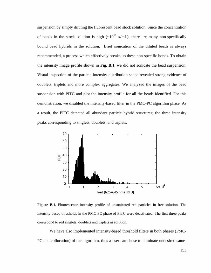
153

suspension by simply diluting the fluorescent bead stock solution. Since the concentration

of beads in the stock solution is high (~1010 #/mL), there are many non-specifically

bound bead hybrids in the solution. Brief sonication of the diluted beads is always

recommended, a process which effectively breaks up these non-specific bonds. To obtain

the intensity image profile shown in Fig. B.1, we did not sonicate the bead suspension.

Visual inspection of the particle intensity distribution shape revealed strong evidence of

doublets, triplets and more complex aggregates. We analyzed the images of the bead

suspension with PITC and plot the intensity profile for all the beads identified. For this

demonstration, we disabled the intensity-based filter in the PMC-PC algorithm phase. As

a result, the PITC detected all abundant particle hybrid structures; the three intensity

peaks corresponding to singlets, doublets, and triplets.

Figure B.1. Fluorescence intensity profile of unsonicated red particles in free solution. The

intensity-based thresholds in the PMC-PC phase of PITC were deactivated. The first three peaks

correspond to red singlets, doublets and triplets in solution.

We have also implemented intensity-based threshold filters in both phases (PMC-

PC and collocation) of the algorithm, thus a user can chose to eliminate undesired same-

154

color particle hybrids during the PITC analysis. See Section. 4.2.4 for details on the

implementation and recommended settings. Automating the intensity-based particle

filtering during the PITC analysis is appropriate for applications where the relevant

physical phenomena are revealed only in a subset of particle hybrids (e.g., monitoring

communication between two cells requires information for two-color cell doublets only).

BINDING INDUCED SPECTRAL LEAKAGE

To eliminate biases associated with particle intensity variations, intensity-based

filters should always be calibrated using measurements performed on the particle image

set being analyzed. One source of variation is associated with changes in the illumination

power, which can cause statistically significant shift in particle intensities measured

between experiments. Another source of variation is associated with spectral leakage of

dual-color particle hybrids. For example, in Figure B.2 we show the PDF of green and

red particles unbound (black) and bound via DNA hybridization (green). See Figure 4.10

for scatter plot of particle (bead) intensities for this experiment.

155

Figure B.2. Binding induced shift in bead fluorescence intensity. Left: Green and red

fluorescence intensity for single beads (black) and bead-bead hybrids (gray). Right: The mean of

green and red bead intensities for unbound, (Ctrl (-)), and bound (Hybrids) samples. The error

bars (indicated inside the markers) represent 99.9% certainty in the mean of bead intensities.

Across several realizations, we saw consistent increase in the emission intensities of the

tracked beads (e.g., green) when they were bound to another bead of a different peak

fluorescence spectra (e.g, red). Since the fluorescence emission of a dye can occur far

from the peak emission wavelength, we hypothesize that the observed increase of

emission intensity of each dye in a two-color bead hybrid is associated with the leakage

of the off-peak fluorescence emission of the other bead in the hybrid. We hypothesize

also that this effect can be decreased by careful selection of color filters.