Embed Size (px)
Citation preview

11
Microeconomics, 2Microeconomics, 2ndnd EditionEdition
David Besanko and Ronald BraeutigamDavid Besanko and Ronald Braeutigam
Chapter 16: General Equilibrium TheoryChapter 16: General Equilibrium Theory
Prepared by Katharine RockettPrepared by Katharine RockettDieter BalkenborgDieter Balkenborg
©© 2006 John Wiley & Sons, Inc.2006 John Wiley & Sons, Inc.

22
�� Trade involves more than one marketTrade involves more than one market
�� General equilibrium model replaced labour theory of General equilibrium model replaced labour theory of value, Debreu: Theory of valuevalue, Debreu: Theory of value
�� Main results in general equilibrium theory:Main results in general equilibrium theory:–– Conditions for the existence of a competitive market equilibriumConditions for the existence of a competitive market equilibrium, ,
i.e., a price system where all markets clear if all agents produi.e., a price system where all markets clear if all agents produce, ce, sell and buy such that they maximize their utility or profits whsell and buy such that they maximize their utility or profits while ile taking all prices as given.taking all prices as given.
–– First welfare theorem: Market equilibria are Pareto efficient inFirst welfare theorem: Market equilibria are Pareto efficient inthe sense that now one can be made better off by a different the sense that now one can be made better off by a different plan of production and a different allocation of goods without plan of production and a different allocation of goods without making anybody else worse off.making anybody else worse off.
–– Second welfare theorem: conversely, every Pareto optimum is a Second welfare theorem: conversely, every Pareto optimum is a market equilibrium for a suitable system of prices and a wellmarket equilibrium for a suitable system of prices and a well--chosen initial allocation of goods chosen initial allocation of goods

33
�� Assumptions needed for the theorems to hold: Assumptions needed for the theorems to hold: –– Homo oeconomicus (individuals must be rational + selfish in the Homo oeconomicus (individuals must be rational + selfish in the
sense their utility only depends on their own consumption)sense their utility only depends on their own consumption)
–– Survival assumptions. Roughly speaking If individuals do not Survival assumptions. Roughly speaking If individuals do not own enough by themselves to survive, a market equilibrium own enough by themselves to survive, a market equilibrium might not exist. might not exist.
–– Convexity assumptionsConvexity assumptions
�� First: Pure barter economy, two goods, two people (e.g. First: Pure barter economy, two goods, two people (e.g. Robinson and Freitag)Robinson and Freitag)–– Edgeworth boxEdgeworth box
–– Description of barterDescription of barter
–– Notion of ParetoNotion of Pareto--efficiencyefficiency
–– The contract curveThe contract curve
–– Market equilibriumMarket equilibrium
–– First and second welfare theoremFirst and second welfare theorem
�� Then: Adding productionThen: Adding production

44
1. For simplicity there are only two individuals and two goods in the economy. Otherwise there could not be any exchange.
2. There is a fixed, total amount of each good in the economy. For now there is no production. Let w1 be the total amount available of commodity one and let w2 be the total amount available of commodity 2.
3. Once these goods are allocated to the two agents, property rights are assigned and we obtain a barter economy if people are allowed to trade freely (or if a black markets can form).

55
� In such a barter economy the agents can voluntarily trade given their initial allocations. Let the initial endowment (or allocation) of Ann (Bob) be wA
1 (wB1) units of good 1 and wA
2 (wB2)
units of good 2. Let (xA1, xA2) and (xB1, xB2) denote the amounts Ann and Bob end up with.
� A feasible allocation is PARETO EFFICIENT if there is no trade from which the two can gain, more precisely, there is no other feasible allocation that makes at least one individual better off and no individual worth off.
66
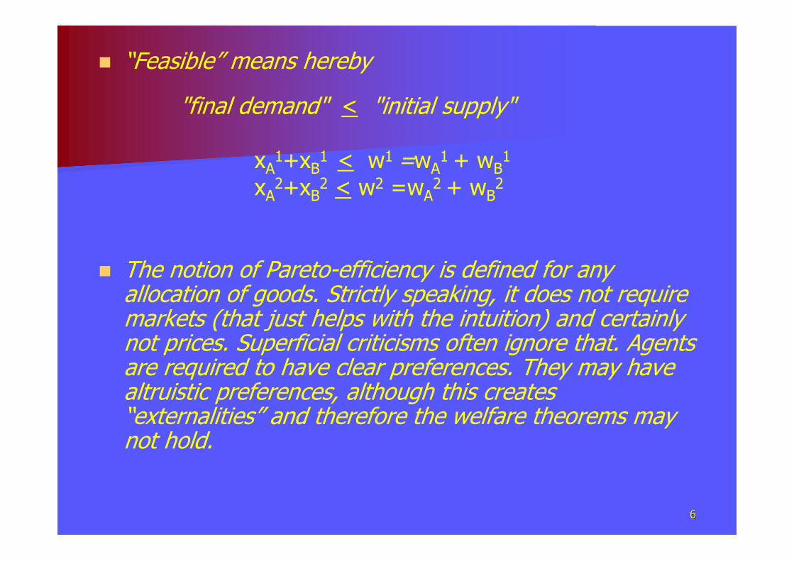
� “Feasible” means hereby
� The notion of Pareto-efficiency is defined for any allocation of goods. Strictly speaking, it does not require markets (that just helps with the intuition) and certainly not prices. Superficial criticisms often ignore that. Agents are required to have clear preferences. They may have altruistic preferences, although this creates “externalities” and therefore the welfare theorems may not hold.
"final demand" < "initial supply"
xA1+xB
1 < w1 =wA1 + wB
1
xA2+xB
2 < w2 =wA2 + wB
2

77
�� Assuming selfish preferences and that no Assuming selfish preferences and that no
commodities are thrown away, we can use commodities are thrown away, we can use
the Edgeworth Box to see whether an the Edgeworth Box to see whether an
allocation is efficient or not. We also allocation is efficient or not. We also
assume the usual shape of the assume the usual shape of the
indifference curves.indifference curves.
�� Any point in the Edgeworth box represents Any point in the Edgeworth box represents
an allocation of the available goods where an allocation of the available goods where
noting is thrown away, as for instance the noting is thrown away, as for instance the
initial allocation E in the following graph.initial allocation E in the following graph.

88Good 1
Good 2
wB2
wB1
Good 2
Good 1
Person A
Person B
wA1
wA2
Example: An Edgeworth Box Diagram
• E
99
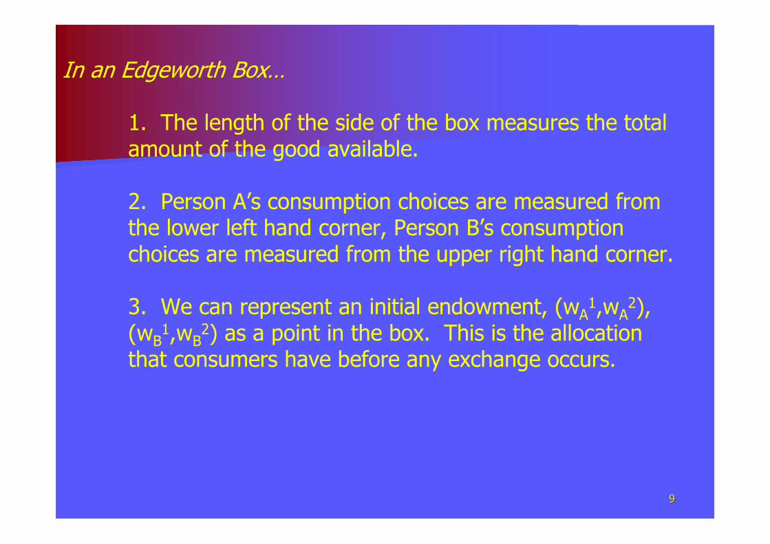
In an Edgeworth Box…
1. The length of the side of the box measures the total amount of the good available.
2. Person A’s consumption choices are measured from the lower left hand corner, Person B’s consumption choices are measured from the upper right hand corner.
3. We can represent an initial endowment, (wA1,wA
2), (wB
1,wB2) as a point in the box. This is the allocation
that consumers have before any exchange occurs.
1010
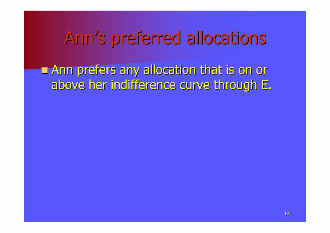
AnnAnn’’s preferred allocationss preferred allocations
�� Ann prefers any allocation that is on or Ann prefers any allocation that is on or
above her indifference curve through E.above her indifference curve through E.

1111Good 1
Good 2
wB2
wB1
Good 2
Good 1
Person A
Person B
wA1
wA2
ICA
Example: An Edgeworth Box Diagram
•E

1212
BobBob’’s preferred allocations preferred allocation
�� For Bob things are reversed. The top right For Bob things are reversed. The top right
corner is the point where he gets nothing. corner is the point where he gets nothing.
Moving down and left. Bob prefers any Moving down and left. Bob prefers any
allocation that is on or below his allocation that is on or below his
indifference curve through E.indifference curve through E.

1313Good 1
Good 2
•E
wB2
wB1
Good 2
Good 1
Person A
Person B
wA1
wA2
ICA
ICB
Example: An Edgeworth Box Diagram
1414
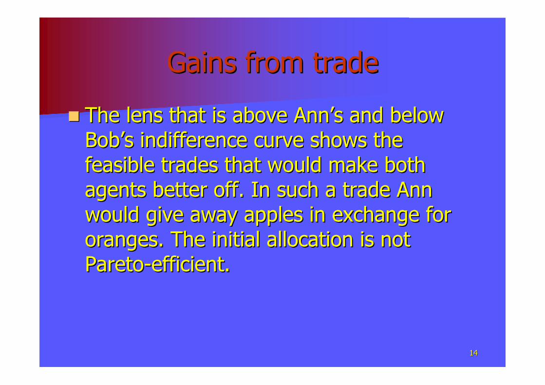
Gains from tradeGains from trade
�� The lens that is above AnnThe lens that is above Ann’’s and below s and below
BobBob’’s indifference curve shows the s indifference curve shows the
feasible trades that would make both feasible trades that would make both
agents better off. In such a trade Ann agents better off. In such a trade Ann
would give away apples in exchange for would give away apples in exchange for
oranges. The initial allocation is not oranges. The initial allocation is not
ParetoPareto--efficient.efficient.

1515Good 1
Good 2
•E
wB2
wB1
Good 2
Good 1
Person A
Person B
wA1
wA2
Example: An Edgeworth Box with an Allocation that could be Improved Upon

1616Good 1
Good 2
•E
wB2
wB1
Good 2
Good 1
Person A
Person B
wA1
wA2
xA1
xA2
xB1
xB2
•
Example: An Edgeworth Box with an Allocation that could be Improved Upon

1717Good 1
Good 2
•E
wB2
wB1
Good 2
Good 1
Person A
Person B
wA1
wA2
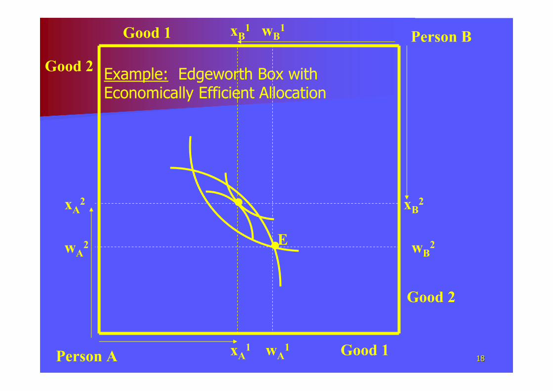
Example: Edgeworth Box with Economically Efficient Allocation
1818Good 1
Good 2
•E
wB2
wB1
Good 2
Good 1
Person A
Person B
wA1
wA2
xA1
xA2
xB1
xB2•
Example: Edgeworth Box with Economically Efficient Allocation

1919Good 1
Good 2
•E
wB2
wB1
Good 2
Good 1
Person A
Person B
wA1
wA2
xA1
xA2
xB1
xB2•M
Example: Edgeworth Box with Economically Efficient Allocation

2020
M
Good 1
Good 2
•E
wB2
wB1
Good 2
Good 1
Person A
Person B
wA1
wA2
xA1
xA2
xB1
xB2•
Example: Edgeworth Box with Economically Efficient Allocation

2121
A ParetoA Pareto--efficient allocationefficient allocation
�� Repeat:Repeat:
�� Is a distribution of the commodities (i.e., Is a distribution of the commodities (i.e.,
an allocation) of the available commodities an allocation) of the available commodities
in such a way that is not possible to in such a way that is not possible to
change the allocation such that at least change the allocation such that at least
one individual is made better off an no one individual is made better off an no
individual is made worth off.individual is made worth off.
�� In other words, there is no reason to tradeIn other words, there is no reason to trade

2222
1. M is Pareto efficient implies in the interior:
2. M is at a tangency point of the two individuals’indifference curves
MRSA1,2 = MRSB1,2
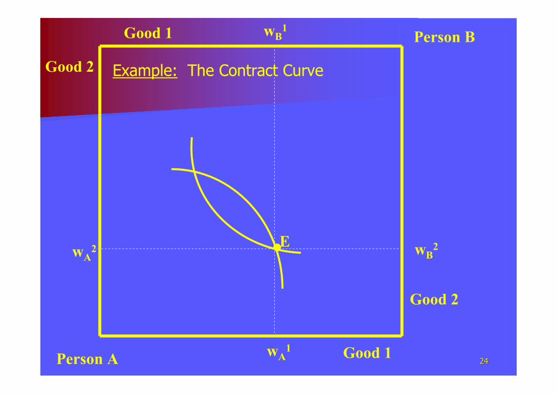
3. Definition: The set of all Pareto efficientpoints in the Edgeworth box is known as the Pareto set or the Contract Curve.
2323
This set typically will stretch from one corner to the other of the box…(M not unique)
A subset of this set will contain the points that are Pareto efficient with respect to the initial endowment.
What is the set of Pareto efficient allocations if there is only one commodity?
2424Good 1
Good 2
•E
wB2
wB1
Good 2
Good 1
Person A
Person B
wA1
wA2
Example: The Contract Curve

2525Good 1
Good 2
•E
wB2
wB1
Good 2
Good 1
Person A
Person B
wA1
wA2
xA1
xA2
xB1
xB2•
Example: The Contract Curve
2626Good 1
Good 2
•E
wB2
wB1
Good 2
Good 1
Person A
Person B
wA1
wA2
xA1
xA2
xB1
xB2•
Example: The Contract Curve

2727Good 1
Good 2
•E
wB2
wB1
Good 2
Good 1
Person A
Person B
wA1
wA2
xA1
xA2
xB1
xB2•
Example: The Contract Curve

2828
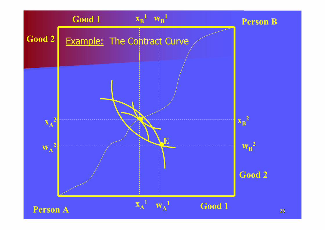
Terminology and findingsTerminology and findings
�� The contract curve consists of the set of The contract curve consists of the set of
all Pareto efficient allocations. At Paretoall Pareto efficient allocations. At Pareto--
efficient allocations inside the Edgeworth efficient allocations inside the Edgeworth
box the agents have identical marginal box the agents have identical marginal
rates of substitution.rates of substitution.
�� An initial endowment E defines a An initial endowment E defines a ““lenslens”” of of
mutually beneficially trades. The mutually beneficially trades. The
intersection of this lens with the contract intersection of this lens with the contract
curve was called the CORE by Edgeworth. curve was called the CORE by Edgeworth.
This is were efficient trade would end. This is were efficient trade would end.

2929
Example: Calculating a Contract Curve
2 individuals, A and B with "Cobb-Douglas" utility functions over 2 goods, X and Y.
UA = (XA)α(YA)
1-α
UB = (XB)β(YB)
1-β

3030
MUYA = (1-α)XA
αY-α
MUXB = βXA
β-1Y1-αβ
MUYB = (1-β)XA
βY-β
XA + XB = 100 …This gives the size of YA + YB = 200 the Edgeworth Box

3131
Therefore,
MRSX,YA = MUX
A/MUYA = [α/(1-α)][YA/XA]
MRSX,YB = MUX
B/MUYB = [β/(1-β)][YB/XB]

3232
And
XA = 100 - XB …feasibility constraints…YA = 200 - YB
MRSX,YA = MRSX,Y
B …tangency conditionfor contract curve…
[α/(1-α)][(200 – YB)/(100 – XB)] = [β/(1-β)][YB/XB]
or

3333
(β-α)YBXB - (1-α)β(100YB) + α(1-β)200XB = 0
or equivalently…
(β-α)YAXA + α(1-β)(100YA) - (1-α)β200XA = 0

3434
B. Draw the contract curve for α = β = ½The equations for the contract curves simplify to:
YA = 2XA and YB = 2XB

3535100
200
XA
B
Contract Curve
Slope = 2
Y
Example: A Contract Curve

3636
The market equilibriumThe market equilibrium
�� Suppose both agents are price takers. (This is Suppose both agents are price takers. (This is
very artificial and would be satisfactory only for very artificial and would be satisfactory only for
many agents.)many agents.)
�� Suppose there are prices Suppose there are prices p1 and and p2..
�� Buy selling his initial endowments each agent Buy selling his initial endowments each agent
can guarantee the incomecan guarantee the income
�� This money can then be used to buy the This money can then be used to buy the
commodity bundle which maximizes utility.commodity bundle which maximizes utility.
2211
AAA wpwpy +=2211
BBB wpwpy +=or

3737
�� If markets then clear, we have a market If markets then clear, we have a market
equilibriumequilibrium
�� If AnnIf Ann’’s optimal demand is s optimal demand is (xA1, xA2) and (xB1, xB2) denote the commodity bundles denote the commodity bundles
that Ann and Bob will buy at the given that Ann and Bob will buy at the given
pricesprices. Then markets clear if the optimal Then markets clear if the optimal
demands define a feasible allocation:demands define a feasible allocation:
"final demand" < "initial supply"
xA1+xB
1 < w1 = wA1 + wB
1
xA2+xB
2 < w2 = wA2 + wB
2

3838Good 1
Good 2
•E
wB2
wB1
Good 2
Good 1
Person A
Person B
wA1
wA2
••
xA1
xA2
xB1
xB2
Example:Prices which do not yield a market equilibrium.
AB

3939Good 1
Good 2
•E
wB2
wB1
Good 2
Good 1
Person A
Person B
wA1
wA2
Example: A Market equilibrium

4040Good 1
Good 2
•E
wB2
wB1
Good 2
Good 1
Person A
Person B
wA1
wA2
xA1
xA2
xB1
xB2•
Example: A Market equilibrium

4141Good 1
Good 2
•E
wB2
wB1
Good 2
Good 1
Person A
Person B
wA1
wA2
-P1/P2
xA1
xA2
xB1
xB2•
Example: A Market equilibrium

4242Good 1
Good 2
•E
wB2
wB1
Good 2
Good 1
Person A
Person B
wA1
wA2
-P1/P2
xA1
xA2
xB1
xB2•
Example: A Market equilibrium

4343
Market equilibriumMarket equilibrium
�� We see: A market equilibrium must be a We see: A market equilibrium must be a
point in the core and hence Paretopoint in the core and hence Pareto--
efficient. This means that the indifference efficient. This means that the indifference
curves of the two agents have the same curves of the two agents have the same
tangent (i.e., both have the same MRS). tangent (i.e., both have the same MRS).
Moreover, this tangent must go through Moreover, this tangent must go through
the initial endowment and hence define the initial endowment and hence define
the budget line for the agents. The latter the budget line for the agents. The latter
implies that the price ratio equals the implies that the price ratio equals the
marginal rate of substitution in marginal rate of substitution in
equilibrium. equilibrium.

4444
�� We have a system of two We have a system of two simultanoeussimultanoeus
equations with two unknowns. The equations with two unknowns. The
existence of a solution is not obvious.existence of a solution is not obvious.
�� General conditions have been worked out General conditions have been worked out
by Arrow, Debreu and by Arrow, Debreu and McKenseyMcKensey. .
Moreover, it follows:Moreover, it follows:

4545
The first welfare theoremThe first welfare theorem
�� Every market equilibrium is ParetoEvery market equilibrium is Pareto--
efficient.efficient.

4646
The second welfare theoremThe second welfare theorem
�� Every Pareto efficient allocation is a market Every Pareto efficient allocation is a market equilibrium for a suitable initial allocation of equilibrium for a suitable initial allocation of commodities.commodities.
Take a point X on the contract curve. Set the Take a point X on the contract curve. Set the relative price such that it is equal to the MRS of relative price such that it is equal to the MRS of the two consumers. Choose as the initial the two consumers. Choose as the initial endowment E a point on the tangent to the endowment E a point on the tangent to the indifference curves. Relative to this initial indifference curves. Relative to this initial endowment the prices and the point X form a endowment the prices and the point X form a market equilibrium. market equilibrium.
Take X=E. Then no consumer wants to trade at Take X=E. Then no consumer wants to trade at these prices and a Market equilibrium is these prices and a Market equilibrium is achieved. We obtain a noachieved. We obtain a no--trade equilibrium.trade equilibrium.

4747Good 1
Good 2
Good 2
Good 1
Person A
Person B
wA1
wA2
-P1/P2
xA1
xA2
xB1
xB2•
Example: A Pareto optimum
X

4848
E
Good 1
Good 2
• wB2
wB1
Good 2
Good 1
Person A
Person B
wA1
wA2
-P1/P2
xA1
xA2
xB1
xB2•
Example: A Market equilibrium
X

4949
This means that society can achieve efficiency by allowing competition…
This equilibrium requires very little information (prices only) or co-ordination.
In fact, any Pareto-efficient equilibrium can be obtained by competition, given an appropriate endowment.
For example, any Pareto efficient allocation, x, can be obtained as a competitive equilibrium if the initial endowment is x.

5050
This means that society can obtain a particularefficient allocation by appropriately redistributing endowments (income).
This can be achieved through taxes/subsidies to endowments (lump sum taxes) that do not affect choice (prices)
In fact, this redistribution could be viewed as the main role of government in the perfectly competitive model
5151
Suppose that all individuals in the economy have a dual role: they are consumers, but they also are the producers. In other words, the individual's role as a producer will determine their income…
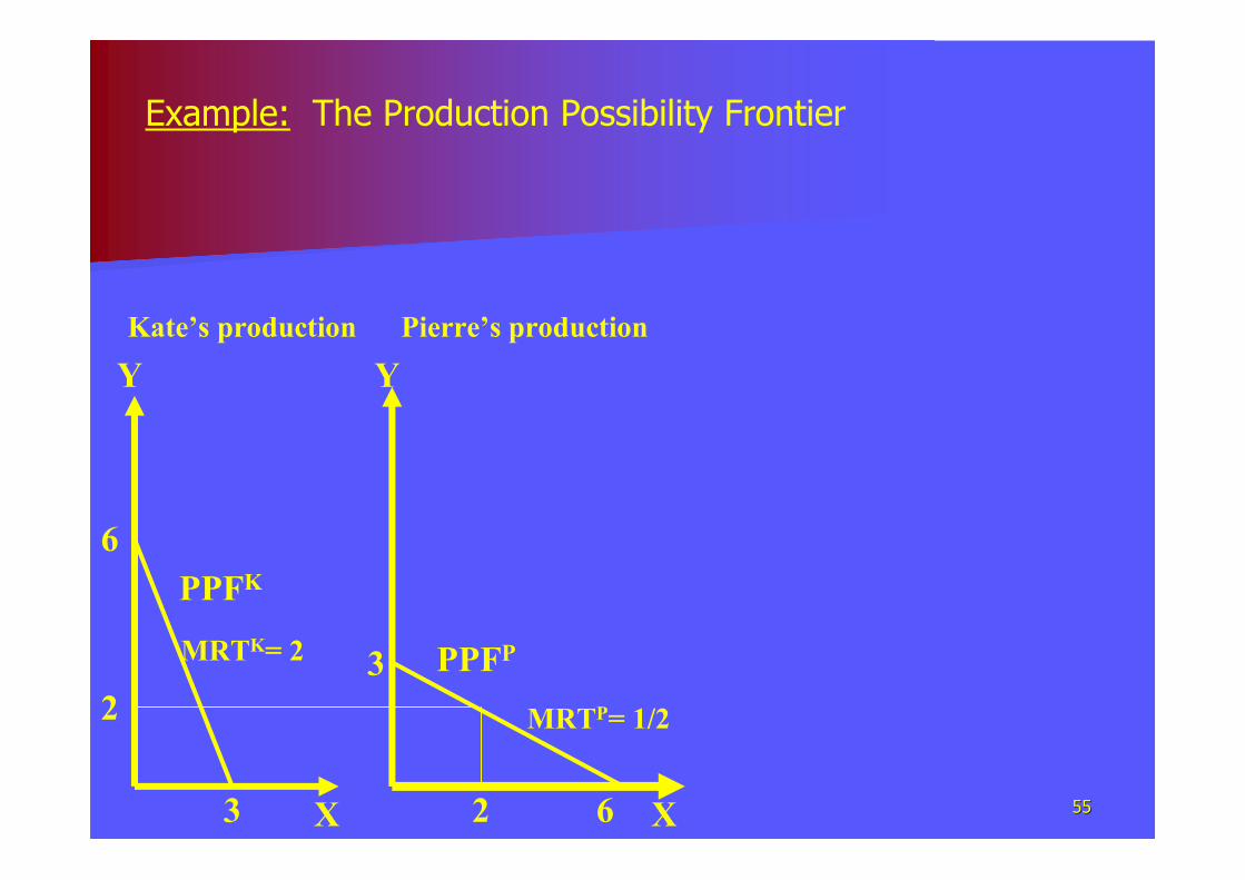
Definition: The production possibility frontier(PPF) of an individual is the maximum combinations of goods A and B that can be produced with the individual’s input (e.g., labor) per unit of time.
Definition: An individual achieves efficiency in production if s/he produces combinations of goods on the PPF (so that there is no "slacking off").
5252
Definition: The slope of the production possibility frontier is the marginal rate of transformation(MRT).
The MRT tells us how much more of good Y can be produced if the production of good X is reduced by a small amount.
Or…the MRT tells us how much it costs to produce one good in terms of foregone production of the other good (opportunity cost).

5353
Y
X
PPF
•
Xs
Slope = -p1e/p2
e
•YeA
XeA
XeB
YeB
Ys
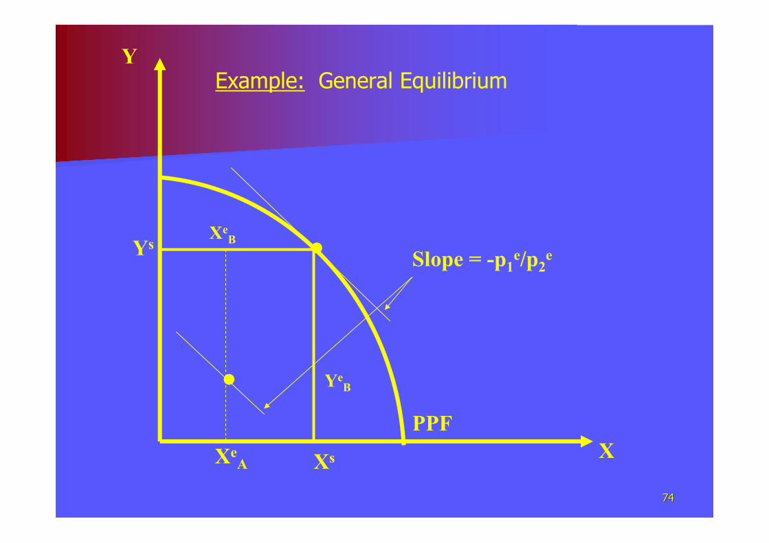
Example: General Equilibrium

5454
Kate’s production
Y
X3
6
2
PPFK
MRTK= 2
Example: The Production Possibility Frontier
5555
Kate’s production Pierre’s production
Y
X
Y
X6
3
3
6
2
2
PPFK
PPFPMRTK= 2
MRTP= 1/2
Example: The Production Possibility Frontier

5656
Kate’s production Pierre’s production Joint Production
Y
X
Y
X
Y
X6
6
6
3
3
6
2
2
PPFK
PPFPMRTK= 2
MRTP= 1/2
MRTJ= 1/2
MRTJ= 2
PPFJ
Example: The Production Possibility Frontier

5757
Definition: The joint PPF for all possible technologies and all producers in the economy depicts the maximum amount of each good that could be produced in total by all producers.
Definition: A producer who, when producing one good, reduces production of a second good less compared to another producer is said to have a comparative advantage in producing the first good.

5858
If the MRT of two different producers (and consumers) differs, then the individuals can potentially gain from trade
If many production methods are available, the joint PPF takes a typically “rounded” shape, representing the various MRT’s available to the economy.

5959
Now, let’s look at the efficient product mix…At which point along the joint PPF would society operate?
Any individual consumer would prefer production to occur at a point where the consumer's indifference curve is just tangent to the PPF.

6060
X
Y
PPFJ
Preference direction
Example: The Efficient Product Mix

6161
X
Y
IC
PPFJ
Preference direction
Example: The Efficient Product Mix
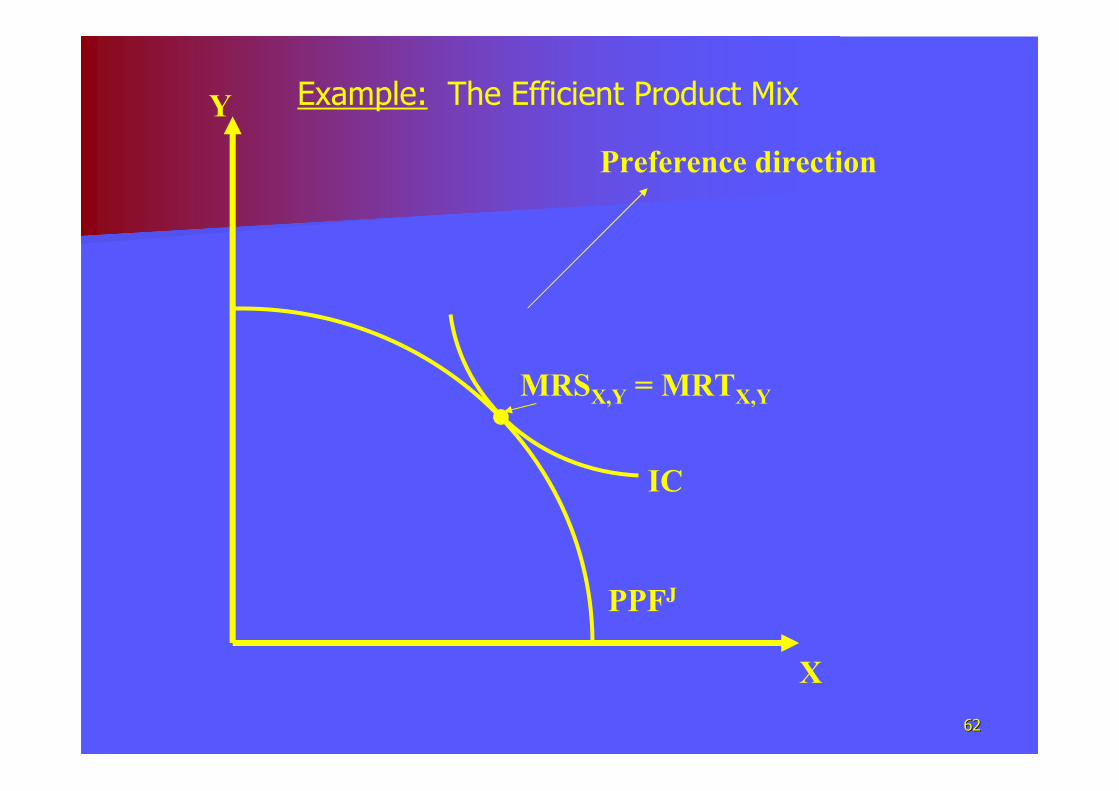
6262
X
Y
•IC
PPFJ
MRSX,Y = MRTX,Y
Preference direction
Example: The Efficient Product Mix
6363
At this point, the consumer’s willingness to give up good X in order to get good Y just equals the rate at which a producer has to give up good X in order to produce more of good Y.
MRTX,Y = MRSX,Y
But…This must be true for all consumers if the economy is to produce optimally for each consumer.

6464
Can the competitive market help us to achieve this optimality?
At the Pareto efficient allocations, it is true for all consumers that:
MRSX,Y = pX/pY

6565
Now, consider the producers’ problem.
Suppose that the producers produce goods X and Y and choose the product mix so as to maximize profits given the prices pXand pY:
Max Π = pXQX + pYQY – C*QX,QY
Where: we will suppose that the cost of production is fixed whatever the optimal output mix (e.g., we just want to know how to employ the labor we have contracted)

6666
Definition: an isoprofit line shows the output combinations that result in a given level of profit, Π0…or…
QY = (Π0 + C*)/pY – pXQX/pY

6767
X
Y
PPFJ
Example: The Profit Maximizing Product Mix

6868
X
Y
•
PPFJ
(ΠΠΠΠ0+C*)/PY
Isoprofit lines
-pX/pY
Example: The Profit Maximizing Product Mix

6969
X
Y
•
PPFJ
Direction of increasing profits
(ΠΠΠΠ0+C*)/PY
Profit maximising product
mix
Isoprofit lines
-pX/pY
Example: The Profit Maximizing Product Mix

7070
Hence, If the firm maximizes profits, then, it chooses the product mix that shifts out the isoprofit line as much as possible while remaining feasible. This is a tangency point such that for all producers:
MRTX,Y = pX/pY

7171
In other words, in equilibrium, the price ratio will measure the opportunity cost of production of one good in terms of production of the other good.
Therefore…
Because competition ensures that both the MRS and the MRT equal the (same) price ratio for all producers and all consumers, a competitive equilibrium achieves an efficient product mix for all producers and all consumers
Our earlier allocative efficiency results still hold with production…

7272
Y
X
PPF
Example: General Equilibrium

7373
Y
X
PPF
•
Xs
XeB
YeB
Ys
Example: General Equilibrium
7474
Y
X
PPF
•
Xs
Slope = -p1e/p2
e
•
XeA
XeB
YeB
Ys
Example: General Equilibrium

7575
Y
X
PPF
•
Xs
Slope = -p1e/p2
e
•YeA
XeA
XeB
YeB
Ys
Example: General Equilibrium

7676
Y
X
PPF
•
Xs
Slope = -p1e/p2
e
•YeA
XeA
XeB
YeB
Ys
Example: General Equilibrium
7777
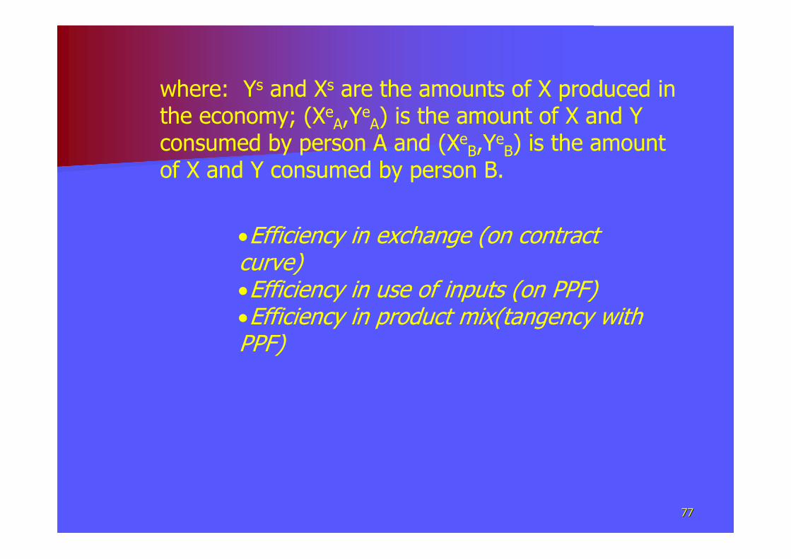
where: Ys and Xs are the amounts of X produced in the economy; (XeA,Y
eA) is the amount of X and Y
consumed by person A and (XeB,YeB) is the amount
of X and Y consumed by person B.
•Efficiency in exchange (on contract curve)•Efficiency in use of inputs (on PPF)•Efficiency in product mix(tangency with PPF)