Microeconomic Uncertainty, International Trade, and AggregateFluctuations�

George Alessandriay

University of RochesterFederal Reserve Bank of Philadelphia and NBER

Horag ChoiMonash University

Joseph P. KaboskiUniversity of Notre Dame and NBER

Virgiliu MidriganNew York University and NBER

Draft: September 2014

AbstractThe extent and direction of causation between micro volatility and business cycles are debated.We examine, empirically and theoretically, the source and e¤ects of �uctuations in the disper-sion of producer-level sales and production over the business cycle. On the theoretical side, westudy the e¤ect of exogenous �rst- and second-moment shocks to producer-level productivity ina two-country DSGE model with heterogenous producers and an endogenous dynamic exportparticipation decision. First-moment shocks cause endogenous �uctuations in producer-level dis-persion by reallocating production internationally, while second-moment shocks lead to increasesin trade relative to GDP in recessions. Empirically, using detailed product-level data in the motorvehicle industry and industry-level data of U.S. manufacturers, we �nd evidence that internationalreallocation is indeed important for understanding cross-industry variation in cyclical patterns ofmeasured dispersion.

JEL classi�cations: E31, F12.Keywords: Sunk cost, establishment heterogeneity, exporting, uncertainty.

�Molin Zhong provided excellent research assistance. We thank Kyle Handley and Hanno Lustig andaudiences at Carnegie-Rochester NYU conference on public policy, EIEF, Emory, The Ohio State Uni-versity, NBER conference on the Macroeconomic Consequeneces of Uncertainty for helpful comments.The views expressed here are those of the authors and do not necessarily re�ect the views of the FederalReserve Bank of Philadelphia or the Federal Reserve System. This paper is available free of charge atwww.philadelphiafed.org/research-and-data/publications/working-papers/.

yCorresponding author: Department of Economics, University Rochester, 204 Harkness Hall Rochester,NY 14627, USA. Tel.: +1 585 275 5252; fax: 585 256 2309.George.Alessandria@Rochester.edu.

1 Introduction

A growing literature attributes an important fraction of cyclical �uctuations in output

to changes in the distribution of idiosyncratic shocks a¤ecting heterogenous producers.

This literature shows in a range of closed economy models that more volatile producer-

speci�c shocks can generate a downturn in economic activity. A primary example is the

Great Recession, during which there was a substantial increase in dispersion of growth

rates across establishments. Still, understanding the extent to which volatility leads to

recessions, or recessions lead to volatility, remains an important task.1 In this paper, we

revisit the relationship between idiosyncratic volatility and business cycles empirically and

theoretically. We do so in the context of an open economy model with non-convex trade

participation decisions across heterogenous producers. Trade models and data constitute a

natural laboratory for examining the role of uncertainty, since the selection into exporting is

well understood. Moreover, �rms rely to di¤erent extents on international trade, so swings

in international trade a¤ect �rms di¤erentially. Additionally, international business cycles

are not perfectly synchronized, so net exports �uctuate in response to country-speci�c

shocks.

On the theoretical side, our analysis focuses on the e¤ects of both �rst- and second-

moment shocks in a variation of the two-country real business cycle model of Backus, Kehoe,

and Kydland (1994) extended to include producer heterogeneity and realistic entry and exit

from the export market as in Alessandria and Choi (2007).2 This model captures the well-

1Bloom (2009) and Bloom et al. (2013) argue that volatility leads to recessions. In Bachmann andMoscarini (2012), recessions lead to experimentation and thus to micro volatility. Bloom (2013) gives anexcellent review of the literature. The work by Decker, D�Erasmo, and Moscoso Boedo (2014) is perhapsthe most relevant to ours. They model endogenous countercyclical volatility through �rm�s choice of thenumber of markets in which to sell. Their empirical measures of markets are industries and the numberand locations of establishments, however.

2The Alessandria-Choi model is a general equilibrium variation of the partial equilibrium model of �rmexport participation in the presence of idiosyncratic and aggregate uncertainty and a sunk export costdeveloped in a series of papers by Baldwin, Krugman, and Dixit to explain the non-linear relationshipbetween the real exchange rate and net exports in the 1980�s. Variations of this model have been shown to

1

known features that (1) not all producers export, (2) those that do are relatively large,

and (3) exporting is quite persistent. We �rst consider the e¤ect of �rst-moment shocks

to the level of productivity on aggregate output and measured producer-level dispersion.

Here we �nd that a home productivity shock (e.g., a recession in the U.S.) will generate

an increase in the dispersion in sales growth across heterogenous producers through two

channels. First, there is a direct cost channel. The country-speci�c shock a¤ects the relative

costs of imported and domestic goods, leading to a reallocation of purchases between the

two and thus an increase in the dispersion of consumer purchases. Second, there is a market

participation channel as domestic producers di¤er in their export participation. A country-

speci�c shock a¤ects non-exporters di¤erently from exporters, leading to a reallocation of

production across these heterogenous producers. Clearly, these channels depend critically

on openness. We show that the model can generate potentially quantitatively important

�uctuations in dispersion.

We use the open economy model to consider the e¤ect of exogenous second-moment3

shocks to producer-level productivity, as studied by Bloom et al. (2013) and Arellano,

et al. (2012) in a closed economy. Contrary to this closed economy literature, we �nd

that a shock increasing producer-level dispersion increases exports. Though the increase in

exports is small, it is two orders of magnitude larger than the impact on output itself, as

higher dispersion allows exporting �rms to export more. Thus, the ratio of trade to GDP

rises. Given that trade fell substantially more than output during the Great Recession,

this constitutes a puzzle for the model.

We next evaluate the importance of �rst-moment shocks on measured producer-level

capture the cross-section and dynamics of export participation of producers in many countries (see Das,Roberts, and Tybout (2007) and Alessandria and Choi (2011a)) as well as the dynamics of trade growth(Alessandria and Choi (2011b).

3Novy and Taylor (2014) examine the role of shocks to aggregate uncertainty on trade �ows in ansS inventory model with higher �xed costs of sourcing abroad than at home as in Alessandria, Kaboski,and Midrigan (2010). Bekes, Fontagne, Murakozy, and Vicard (2014) study how changes in idiosyncraticdemand uncertainty a¤ect the size and frequency of trade �ows. Carballo, Handley and Limao (2014)consider the e¤ect of uncertainty about trade policy on trade in the great trade collapse.

2

dispersion by examining the role of reallocation from international trade in explaining the

increase in dispersion measured by Bloom et al. (2013). We focus narrowly on the cross-

sectional measures of sales and expenditure growth rather than on other measures, such

as the volatility of stock earnings (e.g., Herskovic, Kelly, Lustig, and Van Nieuwerburgh,

2014, and Bloom et al., 2013), which our model is less suited to address.4

At the aggregate level, we �nd that international reallocation is as strongly related to

�uctuations in uncertainty as GDP growth is. Across a wide range of industries, interna-

tional reallocation is an important source of �uctuations in industry-level dispersion over

time. Industries with the largest increase in dispersion are more open both in the narrow

period 2007 to 2009 and in periods of international reallocation more broadly.

Finally, we look within a particular industry, using automobiles as a case study. The

automobile industry is an important industry that had a large and persistent decline in

economic activity during the Great Recession. It is also extremely well measured, allowing

us to look at product-level variation as well as at variation for �rms both within and

outside of the U.S. We �nd that an important share of the increased dispersion in sales

and production from 2008 to 2011 can be attributed to reallocation between the Big 3

�rms and Japanese �rms. This reallocation is driven by identi�able shocks: a spike in oil

prices that has a relatively stronger impact on the Big 3, the pre-bankruptcy crisis and

post-bankruptcy recovery of the Big 3, and the Japanese tsunami which lowered Japanese

sales. Indeed, we �nd that the Japanese tsunami, a clear country-speci�c supply shock,

generates a rise in dispersion of sales and production growth that is nearly as large and

persistent as the rise observed during the Great Recession.

The next section develops and calibrates the two-country model of heterogenous pro-

ducers with an endogenous export decision. In Section 3, we study how the model economy

4Fillat and Garetto (2012) do show that excess stock returns are related to export and multinationalproduction participation and that these di¤erences in returns can be rationalized in a model of with sunkcosts of export participation and multinational production.

3

responds to �rst- and second-moment shocks. Section 4 presents evidence on the relation-

ship between industry volatility and trade reallocation both across industries and within

automobiles, our case study. Section 5 concludes.

2 Model

We describe and calibrate a modi�ed version of the model of Alessandria and Choi (2007),

augmented to allow for idiosyncratic volatility with country speci�c time-varying dispersion.

Speci�cally, there are two symmetric countries, home (H) and foreign (F ), each with a unit

mass of heterogeneous producers producing di¤erentiated intermediate goods. Intermediate

goods producers di¤er exogenously by the variety they produce and their productivity, and

endogenously by their capital and exporter status. Exporting requires both an up-front

cost to start exporting and a �xed continuation cost to stay in the market in subsequent

periods. In each country, competitive �rms produce �nal goods with a CES technology

that combines composites of domestic and imported goods. The domestic composite good

is an aggregate of the full range of domestic intermediates, while the composite imported

good combines only intermediate goods from the subset of the other country�s �rms that

export.

2.1 Intermediate Goods Producers

In each country, a unit mass of monopolistically competitive intermediate goods producers

are indexed by i 2 [0; 1]. Each producer produces output for the domestic market (yH for

home), and potentially an export market (y�H for Home), using a constant returns to scale,

Cobb-Douglas technology. Producers vary in their productivity z:

(1) yH(i) +m0(i)yH(i)� = y(i) = ez(i)eAk(i)�l(i)1��:

4

Here A indicates a (stochastic) aggregate productivity parameter, z (i) is a stochastic

idiosyncratic productivity shock drawn from a process with a time varying country-speci�c

standard deviation of �", k (i) is the producer�s capital stock, and l (i) is the labor used

in production. We denote whether or not a �rm is exporting using the indicator function

m0(i), which equals 1 if the �rm decides to export in the current period and 0 otherwise.

In addition to this exporting decision, intermediate �rms accumulate capital, hire labor,

and set prices. Given inverse demand functions p(yH) and p�(y�H), within-period pro�ts �

depend on productivity, accumulated capital, and the choice of export status:

�(z; k;m0) = maxlp(yH)yH +m0p�(y�H)y

�H �Wtl s:t: (1);

where Wt is the wage.

The export and capital investment decisions,m and x, are dynamic. Capital depreciates

at a rate � and must be purchased in the prior period. Exporting status, m0; is chosen

contemporaneously, but it entails a cost that depends on whether the �rm exported in the

previous period, m. Speci�cally, the cost, f(m), in units of labor, depends on the �rm�s

past export status, m, with f(0) � f(1) > 0. That is, f(0) � f(1) is an up-front (sunk)

cost of entering the export market, while f(1) is a per-period �xed cost of exporting.5

The intermediate �rms choose exports and investment to solve the following dynamic

recursive problem:

V (z;m; k; ) = maxm0;x

�(z; k;m0)�Wtm0f(m)� Px

+EQ0V (z0;m0; x+ (1� �)k; 0) ;

where P is the price of the investment good and Q0 denotes the stochastic discount factor.

5Only the previous period�s export status a¤ects the �xed cost of exporting, so once a producer stopsexporting it must pay f (0) to reenter the market.

5

Here denotes the aggregate state. We assume that E(z0jz) is weakly increasing in

z. The law of motion for idiosyncratic productivity, z, is potentially subject to stochastic

idiosyncratic volatility shocks. If the distribution of idiosyncratic productivity is su¢ ciently

dispersed, the �xed costs of exporting imply that the optimal export decision follows a

threshold rule: export if z � �z(m; k), where �z(m; k) is decreasing in both m and k. The

optimal law of motion for capital also depends on the exporting decision m0 and satis�es

(2) P = E [Q0 [V 0k0 (z

0;m0; k0; 0)]] :

2.2 Final Goods Producers

The demand that intermediate goods producers face comes from the producers of the �nal

goods. There exists a single �nal good in each country that can be used for either con-

sumption or investment. A representative competitive �nal goods producer in each country

aggregates intermediate goods into �nal goods consumption according to an Armington ag-

gregator with a nested constant elasticity of substitution aggregator. For the home �nal

goods producer, the available varieties of intermediates include all domestic varieties but

only the varieties of foreign intermediates of producers that choose to export.

Using home as an example, it is convenient to de�ne the domestic (i.e., home) and

imported (i.e., foreign) aggregates, YH and YF ; separately as follows:

(3) YH =

0@ Xm=f0;1g

Zz;k

ydH (z;m; k)��1� (z;m; k) dkdz

1A ���1

;

and

(4) YF =

0@ Xm=f0;1g

Zz;k

ydF (z;m; k)��1� �(z;m; k)dkdz

1A ���1

;

6

where (z;m; k) and �(z;m; k) denote the measure of home and foreign intermediate

goods �rms, respectively. Note that while the imported goods aggregator is de�ned over

all foreign varieties, demand for foreign varieties that are not exported is constrained to be

zero.

These domestic and imported composites are then aggregated in Armington fashion to

produce �nal consumption, C, and investment goods, x(z;m; k):

(5) C +X

m=f0;1g

Zz;k

x(z;m; k) (z;m; k)dkdz = D =

�Y

�1

H + !1

t Y �1

F

� �1

;

where ! < 1 produces a bias for domestically produced goods. To match the cyclicality

of trade we allow for shocks to !t, !�t in each country. Stockman and Tesar (1995) and

Levchenko, Lewis, and Tesar (2010) �nd these preference shocks to be important determi-

nants of trade �ows.6

Taking the price of �nal goods, P ; intermediate prices, pH(z;m; k), p�H(z;m; k); and

the measures of intermediate �rms as given, the static pro�t maximization of �nal goods

producers yields iso-elastic demand functions for intermediate producers of the form

yH(z;m; k) =

�pH(z;m; k)

PH

��� �PHP

�� Y;

y�H(z;m; k) =

8><>: 0

!�p�H(z;m;k)

P �H

��� �P �HP �

�� Y �

if m0 (z;m; k) = 0

if m0 (z;m; k) = 1;

6Alessandria, Kaboski, and Midrigan (2013) show that these �shocks�may actually primarily re�ectthe di¤erential inventory investment decisions of importers, exporters, and domestic �rms over the busi-ness cycles. For our purposes, we abstract from these endogenous �uctuations in the import preferenceparameters.

7

and the following equilibrium price formulas:

P =�P 1� H + !P 1� F

� 11� ;

PH =

0@ Xm=f0;1g

Zz;k

pH (z;m; k)1�� (z;m; k) dkdz

1A 11��

,

P �H =

0@ Xm=f0;1g

Zz;k

m0 (z;m; k) p�H (z;m; k)1�� (z;m; k) dkdz

1A 11��

:

Given iso-elastic demand, the intermediate goods producers charge a constant markup

over marginal cost:

pH(z;m; k) = p�H(z;m; k) =�

� � 1mc(z;m; k);

where the

mc(z;m; k) =Wl(z;m; k)

(1� �) y(z;m; k):

2.3 Consumer�s Problem

The representative consumer in both countries is in�nitely lived. Given the symmetry, we

develop the home consumer�s problem, and the analogous problem for foreign is denoted

with an asterisk. The home consumer chooses sequences of consumption, Ct, labor, Lt, and

bond holdings, Bt, to maximize expected utility:

VC;0 = maxCt;Lt;Bt

E0

1Xt=0

�tU (Ct; Lt)

8

subject to the sequence of budget constraints,

Ct +QtBt �Wt

PtLt +Bt�1 +

�tPt;

where �t is the sum of pro�ts (net of export costs and capital investment) of the home

country�s intermediate goods producers.

The bond Bt is noncontingent, paying one unit of the home country�s composite �nal

good in period t+ 1; and its price in period t is Qt. An analogous bond exists for foreign.

The Euler equation is therefore

Qt = �EtUC;t+1UC;t

= �EtUC�;t+1UC�;t

P �tP �t+1

Pt+1Pt

;

where Uc;t is the marginal utility of consumption.

2.4 Equilibrium and Computation

The equilibrium de�nition largely follows that in Alessandria and Choi (2007). The distrib-

ution of producers by country over export status, capital, and productivity in each country

is part of the state of the economy ( (z;m; k) ; � (z;m; k)).

In addition, bond holdings and the stochastic levels of TFP, A and A�, are also included

in the aggregate state:

= (B;A;A�; !; !�; �"; ��"; ;

�) ;

where (�"; ��") denote the standard deviation of the idiosyncratic productivity.

9

2.5 Calibration

To perform our quantitative analysis, we need to calibrate the utility function, technologies,

and exogenous stochastic processes for aggregate and idiosyncratic productivity. Our cali-

bration again closely follows that of Alessandria and Choi (2007), with the exception of the

shock process to idiosyncratic productivity z, which here allows for stochastic idiosyncratic

volatility.

We use a constant intertemporal elasticity of substitution utility function that is Cobb-

Douglas in consumption and leisure. Normalizing the time endowment to one, we have

U (C;L) =

�C� (1� L)1��

�1��1� �

We choose standard values for the preference parameters: the discount factor � = 0:96

with a period equaling a year, consistent with an annual return to capital of 4 percent;

logarithmic utility (� = 1); and the share of consumption in utility is chosen so that one-

quarter of non-sleep time is spent working.

For the Cobb-Douglas intermediate goods production functions, we assign � = 0:36,

consistent with standard measures of capital�s share in income. We assign � = 0:1 as the

annual depreciation rate of capital, which is consistent with a steady state capital output

ratio of 2.5. In the �nal goods aggregator, we choose an Armington elasticity = 1:5,

in the midrange of estimates of the elasticity between domestic and imported goods in

the U.S. (Gallaway, McDaniel, and Rivera, 2003). The elasticity of substitution between

varieties is set to 3, so � = 3; and implies a markup of 50 percent over marginal cost.

This structure implies that goods from the same country are better substitutes than goods

from di¤erent countries and is necessary to have some chance of generating reasonable

10

international business cycles.7

We assume that z is drawn from log normal distribution with log mean of zero and

a standard deviation, �". For simplicity, we also assume that these shocks are iid over

time.8 Given this iid structure and the persistent export decision, the optimal capital stock

(determined the period before) will vary simply by whether or not the �rm exported in the

previous period.

The standard deviation for idiosyncratic productivity, �", export costs, f (0) ; f (1) ; and

the home bias parameter, !; jointly determine trade �ows, export participation, exporter

entry and exit, the size of exporters relative to non-exporters, and volatility of producer

growth. We target a trade to GDP ratio of 20 percent, 22 percent of U.S. producers

exporting, and an annualized exit rate from exporting of about 5 percent. The standard

deviation of idiosyncratic shocks a¤ects both the volatility of producer growth and the

exporter premium. With the iid shocks we consider, we cannot simultaneously match

both features of the data. We target instead intermediate values for these moments: an

employment volatility of 16.5 percent (higher than the 10 percent in U.S. Manufacturing,

e.g. Davis, Haltiwanger, and Schuh 1998) and 2.5 exporter premium (lower than the 4.5

ratio in the U.S. Census of Manufacturers).

This calibration yields �" = 0:075; and a ratio of startup export costs to continuation

costs of 1.03, i.e., f(0)=f(1) = 1:03. The ratio of entry costs to continuation costs in this

calibration is relatively low compared to previous estimates in the literature in models

with persistent idiosyncratic shocks (see Das, Roberts, and Tybout, 2007, or Alessandria

and Choi, 2011a). The highly persistent decision to export arises primarily from capital

being predetermined and the slight cost advantage of serving foreign markets with existing

7Having domestic and foreign varieties be equally substitutable leads to business cycles that are notvery synchronized.

8Adding persistence to the z process requires recalibrating the export costs in order to match thepersistence of exporter behavior but, after recalibration, has small impacts on the overall results we present.

11

exporters.9 Given the important �nding of high entry costs, we will also consider versions in

which exporting has more of an investment component. Table 1 summarizes our parameter

values.

Insert Table 1

Figure 1 shows how trade interacts with idiosyncratic productivity shocks to determine

the (log) size distribution. With iid shocks, productivity is log normally distributed. The

top panel shows the distribution of domestic shipments and overall shipments of domes-

tic producers. Domestic shipments are close to log normally distributed, although there

is more mass in the right tail owing to the di¤erent capital stocks of exporters and non-

exporters.10 ;11 The distribution of overall shipments, though, has a fatter right tail than

domestic shipments as more productive producers are more likely to export and hence have

larger sales. The middle panel shows the distribution of purchases by domestic produc-

ers. The distribution of domestic shipments is the same as before. In addition, there is a

distribution of expenditures on imports. The typical importer sells more than the typical

domestic producer. When these distributions are put together again, the distribution of

consumer purchases has more mass in the right tail. Changes in export participation by

domestic and foreign producers will a¤ect the sales and production distributions. The bot-

tom panel shows the distribution of changes in sales and expenditures.12 Both distributions

depart slightly from log-normal. The distribution of sales (shipments by manufacturers)

has more producers that grow/shrink 30 to 50 percent than predicted by the shocks. These

9Without a capital accumulation decision, the same dispersion of productivity shocks and stopper ratewould lead to entry costs that are 66 percent larger than continuation costs.10Recall that exporters with more capital are more likely to continue in the export market, and this

extra capital can contribute to larger sales at home.11The bimodality of the distribution disappears with more dispersion in idiosyncratic shocks.12We calculate growth relative to averages over the two periods. Therefore, for sellers� sales growth

dispersion, foreign exporters who leave the local (i.e., exporting) market are counted as having a declineof -2 while new exporters have sales growth of +2.

12

producers are the ones starting and stopping to export. In general, the model captures the

well-known empirical feature that there is a hierarchy of growth rates related to changes

in export participation (i.e. starters grow faster than continuing exporters who grow faster

than continuing non-exporters who in turn grow faster than stoppers, Bernard and Jensen,

1999; and Alessandria and Choi, 2011a).13

3 Model Experiments

The benchmark model is a steady-state model with no aggregate uncertainty. Into this

model we consider two types of experiments. First, we consider shocks to the �rst moments

of productivity and import preferences that lead to recessions and trade �ows similar to

the data. Second, we study the impact of shocks to the second moment of idiosyncratic

productivity shocks.

3.1 First-moment Shocks

We �rst consider the impact of the business cycle on the dispersion in economic activity

across producers and sellers in the presence of international trade. We ask: How would a

typical U.S. recession a¤ect measured dispersion in the U.S.? The recession is modeled with

a persistent home negative productivity shock (At) along with preference shocks on home

and foreign imports (!t; !�t ). The shock to the preference for imports is included to capture

the well-known cyclical features of trade: Imports tend to fall more than expenditures on

tradable goods, and exports tend to fall less than production of tradables and may even

rise at the start of a recession.14 In this way we can capture how the movements in trade

13The model is consistent with growth premia related to changes in export status at di¤erent horizons.The quantitative �t of the model is slightly better over longer horizons.14The preference shock allows us to address a shortcoming in standard international RBC models, where

imports are less procyclical than in the data while exports are more procyclical. Additionally, importstend not to fall enough in recessions. The relatively large drop in imports is not solely due to trade being

13

�ows give rise to changes in dispersion across home producers and sellers.

Speci�cally we assume shocks to productivity and preferences for imports have a simple

AR(1) formulation:

At+1 = �AAt + "A;t

A�t+1 = �AA�t + "�A;t

ln!t = (1� �!) ln �! + �! ln!t�1 + "!;t

ln!�t = (1� �!) ln �! + �! ln!�t�1 + "�!;t:

We follow much of the literature in setting �A = �! = 0:954: We set "A = �0:05 and hold

productivity constant in foreign ("�A = 0). We then choose "�! so that imports fall twice as

much as production in the �rst period, and set "�! = � "!2to have exports grow slightly.

We follow the emerging literature on micro volatility and report the standard deviation

of growth in producer-level outcomes. We use �sales�to refer to the distribution of total

shipments of home producers (for both domestic use and exports) and �expenditures�when

referring to the distribution of expenditures of home consumers on varieties (both domestic

and imported) available at home.

To �x ideas, we report the results for a model in which the sunk cost of exporting is high

enough to essentially �x export participation along with our benchmark model in which 5

percent of exporters exit each year. The results of the model with no entry and exit from

exporting are presented in Figure 2.

With export participation essentially �xed, a typical recession will tend to temporarily

increase both the dispersion of the growth in sales of domestic producers and the dispersion

of growth of expenditures on goods at home. The increase in domestic shipments is a little

intensive in cyclical goods like capital and durables, but remains even after controlling for composition.Alessandria, Kaboski, and Midrigan (2010) document these dynamics of imports and exports in the U.S.recessions since 1969.

14

over 1 percent, while the increase in expenditures is close to 4.8 percent. The increase

in dispersion of domestic producer shipments growth arises because sales of home non-

exporters fall more than those of exporters, since exports are initially fairly stable. Overall

sales fall about 11.5 percent for the average non-exporters and only 7.4 percent for the

average exporter.

Dispersion in expenditure growth rises by more than dispersion in producer shipments

primarily because expenditures on imports fall more than expenditures on domestically

produced goods. This feature of the model arises because of the presence of preference

shocks. Additionally, stable export sales combined with the predetermined capital stock

implies that non-exporter sales at home actually fall by less than those of exporters, which

adds to the increase in sales growth dispersion (because the cost of production rises more

for exporters than non-exporters).

Figure 3 shows that allowing export participation to respond endogenously to the shocks

increases the change in the dispersion of domestic producer shipments growth from 1 to 2.5

percent.15 The increase arises primarily because the stock of home exporters (denoted N in

the �gure) rises temporarily 16 through an increase in starters (denoted n0) and a reduction

in stoppers (denoted n1). In the model and the data, starters grow faster than continuing

exporters and non-exporters which grow faster than stoppers. The strong initial decline in

imports leads to a decline in the number of foreign exporters driven by a bigger decline in

exit than entry. The decline in foreign exporters is temporary since the aggregate shock

a¤ects only home production, and as the foreign country rebuilds its stock of exporters

(through more entry and less exit) this generates a slightly more persistent increase in

sales dispersion.

15The shocks here have been adjusted to have the same impacts on output, imports, and exports as inthe previous model with exogenous export participation.16This feature of the model is strongly tied to countercyclicality of net exports, which arises in part from

capital accumulation. With capital, real net exports will move into surplus in a recession, as the recessionleads to a reduction in capital investment at home and a slight increase in foreign investment. Withoutcapital, one needs much larger trade costs to generate the countercyclical nature of net exports.

15

3.2 Second-moment Shocks

We next consider the impact of changes in the volatility of shocks to producer-level pro-

ductivity. This sort of shock has featured prominently in the work of Bloom (2009), Bloom

et al. (2013), and Arellano, et al. (2012). Here we �nd that these shocks have a very small

impact on output, but have somewhat larger e¤ects on trade �ows through the selection

e¤ects with endogenous exporting.

As is well known, increasing dispersion will generally increase output in models with

heterogeneous producers (via the Oi-Hartman-Abel e¤ect). As is standard, (Bloom, 2009),

we eliminate this e¤ect by utilizing an aggregate TFP shock that removes this e¤ect in the

closed economy.17 It is assumed that the autoregressive process for �";t is

ln�";t = (1� �) ln�" + � ln�";t�1 + "t:

In keeping with the relatively short-lived movements of volatility measures in the data,

we assume that shocks to volatility are all temporary (� = 0) and unexpected. The country-

speci�c shock increases the volatility of shocks hitting home producers by 10 percent

(" = 0:1) : The results for our benchmark model are plotted in Figure 4. This shock gen-

erates an increase in the dispersion of domestic shipments growth for two periods. There

is very little change in the dispersion of expenditure growth across varieties.18 In the ini-

tial period, producer shipment dispersion grows by almost 11.7 percent, and in the second

period the increase is 2.5 percent. The magni�ed movements in producer shipment dis-

persion arise from the export decision as the more volatile shocks lead to both more entry

and more exit. On net, entry increases slightly (0.2 percent) while exports rise more than

17With the log-normal shocks this entails shift the mean of the productivity shock to � =

��

��11+�(��1)

��2

2 :18This arises primarily because not all producers are hit by the shock and there is some net exit by

foreign exporters from the shock. Eliminating entry and exit would lead to a larger rise in the dispersionin expenditures.

16

double that (0.45 percent). Imports decline slightly, so the country temporarily runs a

slight trade surplus. In the second period, exports and exporters temporarily fall back to

below steady state. Raising the volatility of idiosyncratic shocks primarily a¤ects trade

�ows because the greater dispersion in productivity gives exporters, who tend to be in the

tails, an even greater advantage.

We next consider how sensitive this e¤ect is to the initial productivity advantage of

exporters by considering a case where exporters are larger than in our benchmark. To

implement this, we increase the dispersion in baseline productivity four fold but hold the

stopper rate constant at 5 percent. This case is also of interest because it makes exporting

a more durable decision than in our baseline. To match the same exit rate from exporting

with more volatile idiosyncratic shocks requires the ratio of entry to continuation cost to

rise from about 1.1 to nearly 4, which is more in line with estimates in the literature. This

increases the exporter premium only slightly, from 2.5 to 2.65.

Nonetheless, Figure 5 shows that this larger exporter premium has a substantial im-

pact on the e¤ects of the shock to volatility on both trade �ows and dispersion measures.

Dispersion in sales and expenditures growth now both rise but by less than the shock, even

though entry and exit rise substantially. On net there are fewer exporters, even though ex-

ports rise by almost 2.5 percent. The boom in exports is temporary: by the second period

exports have fallen below steady state as the stock of exporters is also below the steady

state. The dynamics are a bit more prolonged than in our benchmark model because of

the more durable aspect of the export decision.

The central �nding here is that increases in uncertainty primarily a¤ect trade �ows

rather than output. The increase in exports is much larger than the increase in output.

In the case of the slightly larger exporter premium, this increase becomes quantitatively

signi�cant. Unfortunately, such an increase implies counterfactual business cycle patterns.

Empirical patterns show that, while measured producer-level volatility is high in recessions,

17

trade is procyclical, with aggregate trade much more volatile than output. In recessions,

with the Great Recession as a chief example, trade falls and does so precipitously. This

apparent discord between model and empirics constitutes a puzzle for dynamic business

cycle models with extensive export decisions.

3.2.1 Global Uncertainty Shock

Last, we examine the e¤ect of a global rise in idiosyncratic uncertainty on the global

economy. This experiment is motivated by the highly synchronized nature of the Great

Recession. We consider the e¤ects of this shock in our baseline calibration (low) and one

with a larger exporter premium (high) in which there is a larger sunk cost to exporting.

Unlike the country-speci�c increase in uncertainty, the global increase impacts exporters

in both countries symmetrically, highlighting the potential impact on global trade rather

than just movements in trade balances.

Figure 6 shows that a global shock to idiosyncratic volatility raises dispersion in sales

and expenditures a little more than 10 percent. The magni�ed increase in dispersion of

growth rates arises from a slight increase in export participation. The global uncertainty

shock stimulates output and trade, although the increase in output is quite small (about

0.013 percent) while the increase in exports is much larger (0.32 percent).

Turning to the case with a larger exporter premium and more volatile steady-state

idiosyncratic shocks, we �nd that the e¤ects on micro volatility are more muted as the

increases in expenditures and sales are about half of the benchmark case. This muted rise

in dispersion of growth arises because there is now a contraction in export participation.

Despite the reduction in export participation, there is a substantial increase in trade of

almost 3.4 percent and in output of about 0.2 percent.

This case shows that uncertainty shocks may be a potentially important driver of trade

�ows. If micro-level uncertainty shocks were an important factor during the Great Reces-

18

sion, then the research seeking to explain the collapse in trade during this period faces

a potentially larger challenge as these types of shocks can potentially expand trade quite

strongly.

4 Empirical Evidence

The experiment in Section 3.1 suggests that reallocations stemming from country-speci�c

�rst-moment shocks may lead to increases in the dispersion of �rm growth rates. We now

examine whether there is evidence for such mechanisms. We begin by examining whether

the dynamics of changes in industry dispersion measures are associated with aggregate

international reallocations, the absolute values of the change in the real exchange rate or

the net export ratio. We then ask whether variation in openness across industries explains

the cross-industry variation in the dynamics of dispersion. Finally, using detailed data

from the auto industry, we examine whether the composition of output within an industry

is important in explaining the variation in measured dispersion over time.

4.1 All Industries

Our starting point for industry-level analysis is the NBER Industry Uncertainty Data from

Bloom et al. (2013), which gives a cross-sectional measure of annual growth rate variation

across 4-digit SIC industries in the U.S.19 The data are an annual panel. Bloom et al.

examine various industry-level measures, but none are able to signi�cantly explain cross-

industry variation, so the determinants of cross-industry variation are an open question. We

focus on the sample from 1989-2012, since these are the available years for our international

industry-speci�c data that we will utilize later.

In the model, the causal mechanism is clear: the joint shocks to country-speci�c produc-

19These data include the NBER CES manufacturing database.

19

tivity and tastes generate reallocation which leads to an increase in measured dispersion

of �rm growth rates, even if there is no increase in actual micro uncertainty. In these

cross-industry regressions, we do not claim to test causation, but only whether the data

lead to correlations consistent with the theory. Recall that identi�cation of industry-level

correlates in these Bloom et al. data, whether causal or not, represent a contribution.

We begin by examining whether the time variation in industry-level volatility is asso-

ciated with two aggregate measures associated with international reallocation: 1) absolute

changes in the real exchange rate and 2) the absolute change in normalized net exports. We

use the absolute values, since the theory indicates that any change in reallocation will have

heterogeneous e¤ects on �rms, regardless of its sign. For the real exchange rate, we use the

real �e¤ective�(i.e., trade-weighted by country) exchange rate for the U.S. obtained from

the Bank of International Settlements. We look at a one-year lag, since trade is slower

to respond to changes in the real exchange rate, and we construct percentage changes as

�RERt = (RERt�RERt�1)=RERt�1. For net exports, based on current nominal values,

the absolute change in normalized net exports at time t is constructed as

�NXt =

����Xt+1 �Mt+1

Yt+1� Xt �Mt

Yt

���� :We regress the log of the NBER industry sales volatility measure for industry j at time

t on a time trend, industry �xed e¤ects, and these aggregate predictors of volatility (X,

where X represents �RERt, �NXt, and/or, for comparison, real GDP growth at time t):

V salesgrowthj;t = �Xt + �t+ �j + �j;t:

We cluster the standard errors by industry. Here, the estimate of � is of interest.

The results are presented in Table 2.

20

Insert Table 2

Consistent with the theory, in the univariate regressions, the absolute changes in both

the real exchange rate and the net export ratio are associated with increased measured

dispersion in sales growth, and these are signi�cant at the one percent level. The R2 values

indicate that the explanatory power of these regressors is comparable to the explanatory

power of real GDP growth, the more standard explanatory variable for cyclical behavior.

(The R2 values are relatively high, but much of this comes from the industry �xed e¤ects

and the linear time trend.) In the regression that combines all three, GDP growth is the

most signi�cant, but the change in the real exchange rate is still signi�cant at the 5 percent

level, and the change in net exports is marginally signi�cant at the 10 percent level. Thus,

the trade reallocation variables seem to have some additional explanatory power beyond

that of GDP growth alone.

We next examine whether we can explain cross-industry variation in the cyclicality of

dispersion using measures of openness and trade. Recall that trade-driven dispersion in the

model depended critically on the openness of the economy. As an analog here, we examine

the openness of particular industries. We construct these measures of industry openness

using annualized import and export data by HS-code from 1989-2012 from Schott (2008),

aggregated to the 4-digit SIC level. Combining this with industry shipment data from

Bloom et al. (2013), we de�ne the following measures of openness for 4-digit industry j at

21

time t:20

OpenOverallj;t =exportsj;t + importsj;t

shipmentsj:t

OpenImportj;t =importsj;t

(shipmentsj;t � exportsj;t) + importsj;t

OpenExportsj;t =exportsj;t

shipmentsj;t:

We start by focusing on the recent recession. Our motivation is the fact that the

recession was large and was associated with a large collapse and recovery in trade. The

size of the recession is likely to swamp other potential industry-speci�c trends, so our

speci�cation is quite simple.21 We look at whether the absolute change in industry-speci�c

sales volatility from 2009-2007 is correlated with our measures of openness. Note that this

is the drop in the cross-sectional variance of sales growth, not the drop in average sales.

Table 3 presents the results of these regressions. The coe¢ cients on industry openness are

presented in the �rst row, but the exact measure of industry openness varies by column.

Insert Table 3

The coe¢ cients on all three measures of openness are positive and signi�cant, indicating

that openness was associated with larger increases in uncertainty. Since we use the log of

20Merging at the industry, we lose data at several levels. First, the trade data include agriculturalgoods, but these are not included in the NBER data. Second, the concordance between HS and SIC isnot perfect, and we lose many manufacturing industries. Even a cursory examination indicates that this isnot because these industries have zero trade, but is a result of an imperfect concordance. Reconstructinga correspondence goes beyond the task of this analysis. Third, the NBER Industry Uncertainty Datahave fewer industries for reasons unknown. The NBER CES manufacturing database has 459 industries,whereas the NBER Industry Uncertainty Data include 320 to 390 over the years. Schott�s data has 402 to447 sectors.21One potential criticism, especially as it relates to our model, is that while the sources of the Great

Recession are not fully understood, there appears to have been a substantial global element to it. Nonethe-less, we believe our mechanism is more general, in that international reallocation, caused by di¤erences ina broader range of aggregate shocks hitting countries di¤erently, should lead to greater dispersion. It isthis aspect of the mechanism that we evaluate.

22

the uncertainty measure, the coe¢ cient on export openness, for example, indicates that

uncertainty is roughly 1.4 percent higher in an industry that exports all of its shipments

relative to a hypothetical industry that exports none. The magnitude and explanatory

power are substantially larger for import and overall openness than for export openness.

The R2 values are not large for any of the three, but they are comparable to the partial R2

values for the aggregate measures in Table 2.

We now return to the role of the absolute changes in the real exchange rate and net

exports in explaining changes in industry-speci�c uncertainty in the broader time series.

The dependent variable is again the log of the cross-sectional volatility of sales growth in

industry j in year t. However, since our benchmark is an industry-speci�c measure, we use

the industry-speci�c growth in shipments rather than overall GDP growth to control for

change in economic activity. This is shown in the �rst column of Table 3. Total shipment

growth, i.e., the �rst moment, is highly signi�cant. (Although the R2 is high, again most

of this comes from the industry-speci�c �xed e¤ects and the time trend.)

Insert Table 4

Columns two through four show that industry openness alone is not a signi�cant pre-

dictor of volatility in the overall time series as it was during the Great Recession. The

reason may be that both the numerator and denominator of openness change over time

and cyclically. When we add the aggregate real exchange rate (RER) in the third column

and interact it with the industry-speci�c measure of openness, however, we get a positive

and signi�cant coe¢ cient. That is, an absolute change in the real exchange rate seems to

be associated with an increase in cross-sectional volatility, but especially in open industries,

i.e., industries where trade is sizable. Similarly, the fourth column shows that the absolute

change in net exports to GDP is again associated with an increase in cross-sectional volatil-

23

ity. The interaction indicates that this is especially true in industries that are open, but

this term is only marginally signi�cant (at the ten percent level).

We should note the limitations of our explanatory power. Bloom et al. (2013) eval-

uate alternative measures of uncertainty, including volatility of (�rm-level) stock returns.

Their data include three variants of these �nancial uncertainty measures: 1) cross-sectional

variation in stock returns at a point in time, 2) cross-�rm average 12-month variation

in monthly stock returns within a �rm, and 3) variance of pooled (by �rm and month)

monthly returns within a year. Our international reallocation measures are less successful

in explaining cross-industry variation in these �nancial variants. For example, in the re-

gressions in Tables 2 and 3, if we construct our dependent variables using these �nancial

measures rather than those based on sales growth, we do not �nd a relationship with open-

ness (although the aggregate reallocation measures themselves are still signi�cant). This

is not inconsistent with our model; given the forward-looking nature of �nancial prices,

the information in aggregate shocks that leads to more prolonged reallocation dynamics

and di¤erential �rm growth rates may lead to only immediate one-time variation in stock

returns when the shock is realized.

In sum, the results are consistent with the model�s prediction where (1) country-speci�c

shocks lead to increased dispersion because changes in exports and imports lead to realloca-

tion of production, but (2) this happens only when trade plays a quantitatively important

role.

4.2 Autos

Having shown suggestive evidence consistent with the model at the economy-wide and cross-

industry level, we now examine the determinants of measured dispersion within a particular

industry. Similar to Bloom et al. (2013) we �nd that dispersion is high when activity is low,

but consistent with our model, this seems to come in large part from reallocation between

24

domestic and foreign producers rather than among all producers.22 Such reallocation is

consistent with our theoretical �nding from country-speci�c shocks. An advantage of the

auto data are that they more readily identify causality, since the Japanese tsunami was a

well-identi�ed exogenous, country-speci�c shock causing international reallocation.

Data are available on production, yt; and sales, st; of autos in the U.S. at the monthly

level. The data are from Autonews and IHS Automotive and are quite disaggregate (by

company, trim, brand, and product). For each producer, a measure of production and sales

growth is constructed as

�xit = ln (xit=xit�1) :

The standard deviation of this variable, � (�xit) ; is weighted by each �rm�s current-period

share of the variable.23 This measure of dispersion is then logged and seasonally adjusted

using a month dummy. Thus, the dispersion measures can be thought of as the log change

in volatility. Quarterly measures are an average of the monthly measure.

Figure 7 plots the level and volatility of sales and production in a seven-year period

that includes the Great Recession. As is already well known, sales are a bit smoother

than production and fall by less (see Alessandria, Kaboski, and Midrigan, 2013). Indeed,

the drop in production is almost twice that of sales in the �rst two quarters of 2009,

when economic activity was contracting at a fast pace. Figure 7 also plots the change in

the standard deviation of sales and production growth. These two dispersion measures

increase quite substantially as economic activity starts to stagnate in late 2007 (prior to

the start of the recession). Production dispersion rises more initially and surges in 2009.

22Aggregation bias is also a clear driver of rising dispersion as dispersion increases 1) more at the companylevel than product level (i.e., split between truck/SUV and cars) and 2) more at the quarterly level thanthe monthly level.23Unweighted measures are strongly in�uenced by the exit and entry decisions of producers since their

sales growth can be extreme. However, these producers tend to have small market shares in the lead upto exit or period soon after entry.

25

By mid-2010, both measures of volatility have returned to normal levels, while the level of

activity remains quite low. Volatility picks up again at the start of 2011. The increase in

volatility coincides with another country-speci�c shock: the Japanese tsunami.

To clarify the role of reallocation across countries, we consider the reallocation between

the Big 3 and Japanese producers. Speci�cally, let

�ms = 100

xBig3t � xJapant

Xt

� xBig3t�1 � xJapant�1Xt�1

!2;

where Xt is the total production or sales. This is a measure of the amount market share

is being reallocated across country of ownership. Obviously, holding reallocation within

groups constant, more reallocation between the groups will increase the dispersion measure.

Figure 8 plots these dispersion measures for production and sales. The non-seasonally-

adjusted data are plotted. This measure helps clarify that an important source of the rise

in dispersion is predictable and due to the two types of plants having a di¤erent timing of

production. Speci�cally, at year-end and mid-year, there are recurring increases in growth

dispersion. These spikes correspond to the establishments in these periods shutting down

for di¤erent lengths. Once the factories are up and running there is very little dispersion in

growth in the other periods. This point is particularly important since the spike in volatility

in 2009m1 to 2009m7 is larger and more persistent than in the rest of the period. This seems

to correspond to GM and Chrysler experiencing prolonged shutdowns as they reorganized in

early 2009. The monthly sales data tell a similar story: increases in sales growth dispersion

tend to be associated with reallocation between the Big 3 and Japanese brands rather than

within these brands. Comparing reallocation between Big 3 and Japanese producers, there

are much larger swings in production reallocation than sales reallocation at the monthly

level.

To further explore the idea that a rise in dispersion of sales growth re�ects realloca-

26

tions from country or country-industry shocks, Figure 9 plots the quarterly sales growth

dispersion against log change in market share of trucks, imports, Big 3, and Japanese �rms

(all measured as averages of the monthly numbers). The data are not seasonally adjusted.

Clearly, the increase in dispersion in 2008 is accounted for by a shift away from trucks and

the Big 3 toward cars, imports, and Japanese �rms. There are two clear phases to this

reallocation in 2008 and 2009. In 2011, sales growth dispersion again rises sharply. This

rise re�ects a shift away from sales of Japanese cars (produced in the U.S. or imported) as

the tsunami in Japan had a much larger e¤ect on Japanese �rms�sales of cars produced in

the U.S. and Japan.

5 Conclusions

Using quantitative theory and data, we have examined 1) the impact of aggregate inter-

national shocks on measured producer-level volatility or dispersion through the channel of

international trade, and 2) the impact of stochastic micro-level volatility on the cyclical

patterns of international trade and output.

Examination of the �rst channel uncovered a potentially important source of measured

cyclicality in �rm-level dispersion: shocks that a¤ect international trade patterns increase

sales growth dispersion. The model indicates that such a channel could be quantitatively

important, and our empirical evidence shows that industry volatility measures are indeed

associated with measures of trade reallocation shocks and measures of openness. Moreover,

within the auto industry, through careful investigation, we have con�rmed the importance of

such country-to-country reallocation at the �rm level. Examination of the second channel,

in contrast, uncovered a puzzle for the standard business cycle model used to understand

micro-level trade dynamics: Increases in �rm-level dispersion lead to large increases in

trade rather than the steep declines typically observed during recessions.

27

The �rst channel we have uncovered motivates several avenues for future research. First,

although autos represent an important industry, it would be informative to examine whether

other industries behave in a similar fashion. This would require access to comprehensive

�rm-level data.

Second, although trade-induced reallocation appears to be an important channel, it

doesn�t appear to be the entire story. Recall that we are not able to explain cross-industry

variation in the volatility of stock returns. Similarly, the mechanism may also have little

to say about neither the implied volatility of a 30-day option (i.e., Chicago Board Options

Exchange Market Volatility Index, or VIX) that Bloom (2009) examines, nor the di¤erences

in aggregate predictions and greater dispersion in �rm-level forecast errors documented by

Bachmann, Elstner, and Sims (2013). These two empirical patterns may both primarily

re�ect aggregate uncertainty, and, of course, even �rm-level business cycle dynamics from

country-speci�c shocks would presumably be predictable. In any case, a quantitative de-

composition of the fraction of cyclical changes in dispersion that can be explained by trade

reallocations remains to be done.

Our analysis is a starting point for examining the impact of country-speci�c shocks

on cyclical �uctuations in producer level dispersion. We undertake this in a benchmark

model that captures the key di¤erences in producer heterogeneity and export participation.

Future quantitative work should take into account the di¤erences in international input

usage, the high share of durables and capital goods in trade, and additional shocks to trade

or monetary policy.

Finally, aggregate uncertainty in trade policy may itself be important to business cycle

and trade dynamics. A quantitative analysis of this channel is the subject of our ongoing

work.

28

References

Alessandria, G. and H. Choi, 2007. �Do Sunk Costs of Exporting Matter for Net ExportDynamics?�Quarterly Journal of Economics, 122(1), 289-336.

Alessandria, G. and H. Choi, 2011a. �Establishment Heterogeneity, Exporter Dynamics,and the E¤ects of Trade Liberalization,�Federal Reserve Bank of Philadelphia WorkingPaper.

Alessandria, G. and H. Choi, 2011b. �Do Falling Iceberg Costs Explain Recent US ExportGrowth�Federal Reserve Bank of Philadelphia Working Paper.

Alessandria, G., J.P. Kaboski, and V. Midrigan. 2010. �The Great Trade Collapse of 2008�09: An Inventory Adjustment?�IMF Economic Review, 58(2): 254-94.

Alessandria, G., J. Kaboski, and V. Midrigan, 2013. �Trade Wedges, Inventories, andInternational Business Cycles,�Journal of Monetary Economics, 60(1), 1-20.

Alessandria, G., H. Choi, J. Kaboski, and V. Midrigan, 2014. �Aggregate E¤ects of TradePolicy Uncertainty,�mimeo.

Arellano, C. Y. Bai, and P. Kehoe, 2012. �Financial Markets and Fluctuations in Uncer-tainty,�mimeo.

Bachmann, R. and G. Moscarini, 2012. �Business Cycles and Endogenous Uncertainty�,Yale mimeo.

Bachmann, R., S. Elstner, and E. Sims, 2013. �Uncertainty and Economic Activity: Ev-idence from Business Survey Data,�American Economic Journal: Macroeconomics, 5(2):217-49.

Bekes, G., L. Fontagne, B.Murakozya, and V. Vicard, 2014. �Shipment Frequency of Ex-porters and Demand Uncertainty�mimeo.

Bernard, A.B. and J.B. Jensen, 1999. �Exceptional Exporter Performance: Cause, E¤ect,or Both?�Journal of International of Economics, 47(1), 1-25.

Bloom, N., M. Floetotto, N. Jaimovich, I. Saporta-Eksten, and S. Terry, 2013. �ReallyUncertain Business Cycles,�Econometrica, forthcoming.

Bloom, N., 2009. �The Impact of Uncertainty Shocks.�Econometrica, May 77, pp. 623-685.

Bloom, N., 2013. �Fluctuations in Uncertainty,�Journal of Economic Perspectives.

Backus, D., P. Kehoe, and F. Kydland, 1994. �Dynamics of the Trade Balance and theTerms of Trade: The J Curve?�American Economic Review, LXXXIV 84�103.

29

Carballo, J., K. Handley and N. Limao, 2014. �Trade Collapse and Policy Uncertainty inthe Great Recession,�mimeo.

Davis, S., J. Haltiwanger and S. Schuh, 1998. Job Creation and Destruction. The MITPress.

Das, S., M. Roberts, and J. Tybout, 2007. �Market Entry Costs, Producer Heterogeneity,and Export Dynamics,�Econometrica, 75(3), 837-73.

Decker, R., P. D�Erasmo, and H. Moscoso Boedo, 2014. �Market Exposure and EndogenousFirm Volatility,�mimeo.

Fillat, J. and S. Garetto, 2012. �Risks, Returns, and Multinational Production,�mimeo.

Gallaway, M.P., C.A. McDaniel, and S.A. Rivera, 2003. �Short-Run and Long-RunIndustry-Level Estimates of U.S. Armington Elasticities,�North American Journal of Eco-nomics and Finance, 14(1), 49-68.

Herskovic, B., B. Kelly, H. Lustig, and S. Van Nieuwerburgh, 2014. �The Common Factorin Idiosyncratic Volatility: Quantitative Asset Pricing Implications,�mimeo.

Levchenko, Andrei A., Logan T. Lewis and Linda L. Tesar, 2010. �The Collapse of Interna-tional Trade During the 2008-2009 Crisis: In Search of the Smoking Gun,�IMF EconomicReview, 58(2): 214-53.

Schott, P., 2008. �The Relative Sophistication of Chinese Exports,�Economic Policy, 5,5-49.

Stockman, A. and L. Tesar, 1995. �Tastes and Technology in a Two-Country Model ofthe Business Cycle: Explaining International Comovements,�American Economic Review,85(1), 168-85.

Taylor, A. and D. Novy, 2014. �Trade and Uncertainty,�NBER Working Paper 19941.

30

Table 1: Parameter ValuesCommon � � � � �

1 1.5 3 0.96 0.36 0.10

�" f0=f1 ! �Benchmark 0.075 1.03 0.3659 0.3592High Dispersion 0.30 1.66 0.3603 0.3599

Table 2: Industry-level Dispersion and Aggregate Reallocation (1989 - 2011)GDP Growth �RER �Net Exports All 3

GDP Growth -0.005��� . . -0.005���

0.002 . . 0.002�RER . 0.265�� . 0.247��

. 0.113 . 0.113�Net Exports . 1.296��� 0.841�

. 0.512 0.486R2 0.61 0.61 0.61 0.61Observations 5088 5088 5088 5088Note: �;�� ; and ��� denote signi�cance at 10, 5, and 1 percent levels, respectively. Standarderrors are below each coe¢ cient and are clustered by industry.

31

Table 3: Industry-level Dispersion and Industry Openness (2007 - 2009)Overalljt Importj;t Exportj;t

Industry Openness 0.034��� 0.040�� 0.014��

0.011 0.011 0.005R2 0.05 0.07 0.03Observations 195 193 195Note: �;�� ; and ��� denote signi�cance at 10, 5, and 1 percent levels, respectively. Standarderrors are below each coe¢ cient.

Table 4: Industry-level Dispersion, Aggregate Reallocationand Openness (1989 - 2011)

�Industry Industry �RER �Net ExportsShipments Openness Interact Interact

�Shipments -0.236��� . . .0.028 . . .

Openness . 0.010 0.007 0.006. 0.011 0.011 0.012

�RER . . 2.392��� .. . 0.756 .

�RER x Open . . 0.773�� .. . 0.375 .

�NX . . . 0.549���

. . . 0.164�NX x Open . . . 0.135�

. . . 0.071R2 0.64 0.64 0.63 0.63Observations 4840 4840 4840 4840Note: �;�� ; and ��� denote signi�cance at 10, 5, and 1 percent levels, respectively. Standarderrors are below each coe¢ cient and are clustered by industry.

32

Figure 1: Distributions 20 Percent Trade

­3.2 ­3 ­2.8 ­2.6 ­2.4 ­2.2 ­2 ­1.8 ­1.6 ­1.40

0.5

1

1.5

2

2.5

3

3.5

4

Log sales

Den

sity

Home Producer Shipment Distribution

Mfr ShipmentsMfr Domestic Shipments

­3.2 ­3 ­2.8 ­2.6 ­2.4 ­2.2 ­2 ­1.80

0.5

1

1.5

2

2.5

3

3.5

4

4.5

5

Log sales

Den

sity

Home Consumer Purchase Distribution

DomesticImportsAll

­2 ­1.5 ­1 ­0.5 0 0.5 1 1.5 20

0.5

1

1.5

2

2.5

3

3.5

Den

sity

Sales Distribution

SalesExpenditures

33

Figure 2: Home Recession: Exogenous Export Participation

0 4 8 12 160

2

4

6

year

Perc

ent c

hang

eStd(Sales Growth)Std(Expenditure Growth)

0 4 8 12 16­20

­10

0

10

year

Perc

ent c

hang

e

Std(Sales)Std(Expenditure)

0 4 8 12 16­10

­5

0

5

year

Perc

ent c

hang

e

Y growthY* growth

0 4 8 12 16­10

­5

0

5

year

Perc

ent c

hang

e

YY*

0 4 8 12 16­15

­10

­5

0

5

year

Perc

ent c

hang

e

NonX sales growthX sales growth

0 4 8 12 16­30

­20

­10

0

10

year

Perc

ent c

hang

e

NonX E growthX E growthFX E growth

0 4 8 12 16­15

­10

­5

0

5

year

Perc

ent c

hang

e

EXIMTBY

34

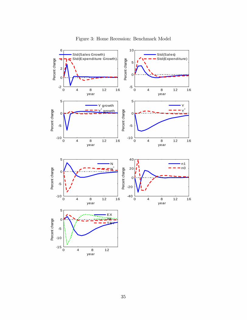
Figure 3: Home Recession: Benchmark Model

0 4 8 12 16­2

0

2

4

6

year

Perc

ent c

hang

eStd(Sales Growth)Std(Expenditure Growth)

0 4 8 12 16­5

0

5

10

year

Perc

ent c

hang

e

Std(Sales)Std(Expenditure)

0 4 8 12 16­10

­5

0

5

year

Perc

ent c

hang

e

Y growthY* growth

0 4 8 12 16­10

­5

0

5

year

Perc

ent c

hang

e

YY*

0 4 8 12 16­10

­5

0

5

year

Perc

ent c

hang

e

NN*

0 4 8 12 16­40

­20

0

20

40

year

Perc

ent c

hang

e

n1n0

0 4 8 12­15

­10

­5

0

5

year

Perc

ent c

hang

e

EXIMTBY

35

Figure 4: Home Uncertainty Shock

0 4 8 12 16­5

0

5

10

15

year

Perc

ent c

hang

eStd(Sales Growth)Std(Expenditure Growth)

0 4 8 12 16­2

0

2

4

6

year

Perc

ent c

hang

e

Std(Sales)Std(Expenditure)

0 4 8 12 16­0.02

0

0.02

0.04

year

Perc

ent c

hang

e

Y growthY* growth

0 4 8 12 16­0.02

0

0.02

0.04

year

Perc

ent c

hang

e

YY*

0 4 8 12 16­0.1

0

0.1

0.2

0.3

year

Perc

ent c

hang

e

NN*

0 4 8 12 16­20

0

20

40

60

year

Perc

ent c

hang

e

n1n0

0 4 8 12­0.2

0

0.2

0.4

0.6

year

Perc

ent c

hang

e

EXIMTBY

36

Figure 5: Home Uncertainty Shoc: High Export Premium

0 4 8 12 16­5

0

5

10

year

Perc

ent c

hang

eStd(Sales Growth)Std(Expenditure Growth)

0 4 8 12 16­5

0

5

10

year

Perc

ent c

hang

e

Std(Sales)Std(Expenditure)

0 4 8 12 16­0.1

0

0.1

0.2

0.3

year

Perc

ent c

hang

e

Y growthY* growth

0 4 8 12 16­0.1

0

0.1

0.2

0.3

year

Perc

ent c

hang

e

YY*

0 4 8 12 16­0.6

­0.4

­0.2

0

0.2

year

Perc

ent c

hang

e

NN*

0 4 8 12 16­20

0

20

40

60

year

Perc

ent c

hang

e

n1n0

0 4 8 12­1

0

1

2

3

year

Perc

ent c

hang

e

EXIMTBY

37

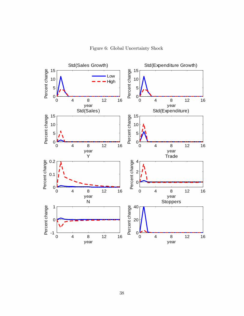
Figure 6: Global Uncertainty Shock

0 4 8 12 160

5

10

15Std(Sales Growth)

year

Perc

ent c

hang

e

LowHigh

0 4 8 12 160

5

10

15Std(Expenditure Growth)

year

Perc

ent c

hang

e

0 4 8 12 160

5

10

15Std(Sales)

year

Perc

ent c

hang

e

0 4 8 12 160

5

10

15Std(Expenditure)

year

Perc

ent c

hang

e

0 4 8 12 160

0.1

0.2Y

year

Perc

ent c

hang

e

0 4 8 12 16­1

0

1N

year

Perc

ent c

hang

e

0 4 8 12 160

20

40Stoppers

year

Perc

ent c

hang

e

0 4 8 12 16

0

2

4Trade

year

Perc

ent c

hang

e

38

Figure 7: Volatility and Level of Activity (Sales and Production of Autos)­1

­.50

.51

log 

Cha

nge

2005q1 2006q1 2007q1 2008q1 2009q1 2010q1 2011q1 2012q1quarter

Sales Volatility Production VolatilitySales Production

39

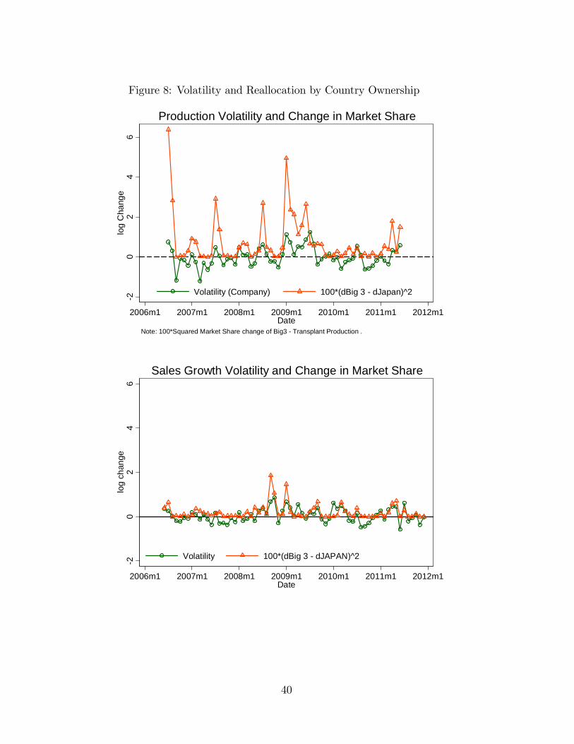
Figure 8: Volatility and Reallocation by Country Ownership

­20

24

6lo

g C

hang

e

2006m1 2007m1 2008m1 2009m1 2010m1 2011m1 2012m1Date

Volatility (Company) 100*(dBig 3 ­ dJapan)^2

Note: 100*Squared Market Share change of Big3 ­ Transplant Production .

Production Volatility and Change in Market Share­2

02

46

log 

chan

ge

2006m1 2007m1 2008m1 2009m1 2010m1 2011m1 2012m1Date

Volatility 100*(dBig 3 ­ dJAPAN)^2

Sales Growth Volatility and Change in Market Share

40

Figure 9: Sales Volatility and Market Shares

­.50

.51

log 

Cha

nge

2005q1 2006q1 2007q1 2008q1 2009q1 2010q1 2011q1 2012q1quarter

Sales Volatility ImportsTrucks Big3Japan

Note: Data are not seasonally adjusted.Market shares are log deviations from pre­recession mean.

41