Embed Size (px)
Citation preview

1
Microeconomic Theory
The Course:
• This is the first rigorous course in microeconomic
theory
• This is a course on economic methodology.
• The main goal is to teach analytical tools that will
be useful in other economic and business courses

2
Microeconomic Theory
Microeconomics analyses the behavior of individual
decision makers such as consumers and firms.
Three key elements:
1. Household choices (consumption, labor supply)
2. Firm choices (production)
3. Market interaction determines prices/quantities

3
Everyday Economics
Economics provides a universal framework
• Applies to different countries
• Applies to different goods
Examples:
• Should you come to class or stay in bed?
• What should you eat for breakfast?
• Should you commit a crime?
Economics:
• Maximizing behavior

4
Example: Your trip to class
How do you get here?
• Car - cost of car, gas, parking.
• Bus – cost of fare, time cost.
What if gas prices rise?
• I don’t care about prices: full tank
• Take bus instead.
Economics:
• Income effect.
• Substitution effect.

5
Example: How do you finance college?
How raise money?
• Job – graduate without debt.
• Borrow – higher wages later, perform better.
What if fees rise?
• Start job – have to borrow less
• Quit job – take econ classes instead of art
Economics:
• Labor supply decision.
• Engel curves

6
Example: At Home
Puzzle:
• In the winter, why are houses in LA colder
than those in Chicago?
Heating decision:
• Chicago – insulate house, buy giant heater.
• Los Angeles – small space heater.
Economics:
• Technology choice.
• Fixed vs. marginal costs.

7
Microeconomic Models
A model is a simplification of the real world.
• Highlights key aspects of problem
• Use different simplifications for different problems.
Example: consumer’s choose between
• Two consumption goods
• Consumption and leisure
• Consumption in two time periods.

8
Aspects of Models
Qualitative vs. Quantitative
• Qualitative – isolates key effects
• Quantitative – estimate size of effects
Positive vs. Normative
• Positive – make predictions
• Normative – evaluate outcomes, make predictions.
How to evaluate a model?
• Test assumptions – are premises reasonable?
• Test predictions – is model accurate?

9
Ingredients in Economic Models
1. Agents have well specified objectives
• Consumers, Firms
2. Agents face constraints
• Money, technology, time.
3. Equilibrium
• Agents maximize given behavior of others.

10
Chapter 2
THE MATHEMATICS OF
OPTIMIZATION

11
The Mathematics of Optimization
• Why do we need to know the mathematics
of optimization?
• Consumers attempt to maximize their
welfare/utility when making decisions.
• Firms attempt to maximizing their profit
when choosing inputs and outputs.

12
Maximization of a Function of
One Variable• The manager of a firm wishes to
maximize profits:
)(qf
= f(q)
Quantity
*
q*
Maximum profits of
* occur at q*

13
Maximization of a Function of
One Variable
= f(q)
Quantity
*
q*
1
q1
0
q
• If the manager produces less than q*, profits
can be increased by increasing q:
– A change from q1 to q* leads to a rise in

14
Maximization of a Function of
One Variable• If output is increased beyond q*, profit will
decline
– an increase from q* to q3 leads to a drop in
= f(q)
Quantity
*
q*
0
q3
q3

15
Derivatives
• The derivative of = f(q) is the limit of
/q for very small changes in q
h
qfhqf
dq
df
dq
d
h
)()(lim
0
• The value of this ratio depends on the
value of q

16
Value of a Derivative at a Point
• The evaluation of the derivative at the
point q = q1 can be denoted
1qqdq
d
• In our previous example,
0
1
qqdq
d0
3
qqdq
d0
*qqdq
d

17
First Order Condition
• For a function of one variable to attain
its maximum value at some point, the
derivative at that point must be zero
0 *qq
dq
df

18
Second Order Conditions
• The first order condition (d/dq) is a
necessary condition for a maximum, but
it is not a sufficient condition
Quantity
*
q*
If the profit function was u-shaped,
the first order condition would result
in q* being chosen and would
be minimized

19
Second Order Condition
• The second order condition to represent
a maximum is
0)("*
*
2
2
qfdq
d
• The second order condition to represent
a minimum is
0)("*
*
2
2
qfdq
d

20
Functions of Several Variables
• Most goals of economic agents depend
on several variables
• In this case we need to find the
maximum and minimum of a function of
several variables:
),...,,( nxxxfy21

21
Partial Derivatives
1
11
1ff
x
f
x
yx or or or
• The partial derivative of the function f
with respect to x1 measures how f
changes if we change x1 by a small
amount and we keep all the other
variables constant.
• The partial derivative of y with respect
to x1 is denoted by

22
• A more formal definition of the partial
derivative is
Partial Derivatives
h
xxxfxxhxf
x
f nn
h
),...,,(),...,,(lim
2121
01

23
Second-Order Partial Derivatives
• The partial derivative of a partial
derivative is called a second-order
partial derivative
ij
jij
i fxx
f
x
xf
2)/(

24
Young’s Theorem
• Under general conditions, the order in
which partial differentiation is conducted
to evaluate second-order partial
derivatives does not matter
jiij ff

25
Total Differential
• Suppose that y = f(x1,x2,…,xn)
• We want to know by how much f changes if
we change all the variables by a small
amount (dx1,dx2,…,dxn )
• The total effect is measured by the total
differential
n
n
dxx
fdx
x
fdx
x
fdy
...
2
2
1
1
nndxfdxfdxfdy ...2211

26
First-Order Conditions
• A necessary condition for a maximum (or
minimum) of the function f(x1,x2,…,xn) is
that dy = 0 for any combination of small
changes in the x’s
• The only way for this to be true is if
0...21 nfff

27
• To find a maximum (or minimum) we have to
find the first order conditions:
f/x1 = f1 = 0
f/x2 = f2 = 0
.
f/xn = fn = 0
.
.
First-Order Conditions

28
Second Order Conditions -Functions of Two Variables
• The second order conditions for a
maximum are:
– f11 < 0
– f22 < 0
– f11 f22 - f122 > 0

29
CONSTRAINED MAXIMIZATION

30
Constrained Maximization
• What if all values for the x’s are not
feasible?
– the values of x may all have to be positive
– our choices are limited by the amount of
resources/income available
• One method used to solve constrained
maximization problems is the Lagrangian
multiplier method

31
Lagrangian Multiplier Method
• Suppose that we wish to find the values
of x1, x2,…, xn that maximize
y = f(x1, x2,…, xn)
subject to a constraint that permits only
certain values of the x’s to be used
g(x1, x2,…, xn) = 0
In our example:
m-p1x1-p2x2-p3x3…-pnxn = 0

32
Lagrangian Multiplier Method
• First, set up the following expression
L = f(x1, x2,…, xn ) + g(x1, x2,…, xn)
• where is an additional variable called a Lagrangian multiplier
• L is often called the Lagrangian
• Then apply the method used in absence of the constraint to L

33
Lagrangian Multiplier Method
• Find the first-order conditions of the
new objective function L:
L/x1 = f1 + g1 = 0
L/x2 = f2 + g2 = 0
.
L/xn = fn + gn = 0
.
.
L/ = g(x1, x2,…, xn) = 0

34
Lagrangian Multiplier Method
• The first-order conditions can generally
be solved for x1, x2,…, xn and
• The solution will have two properties:
– the x’s will obey the constraint:
g(x1, x2,…, xn) = 0
– these x’s will make the value of L as large
as possible
– since the constraint holds, L = f and f is also
as large as possible

35
Interpretation of the Multiplier
• measures how much the objective function f
increases if the constraint is relaxed slightly
• Consumption example:
– represents the increase in utility if we increase
income a little.
– Poor people - high
– Rich people – low
– If =0 then the constraint is not binding

36
Interpretation of Lagrangian
• The Lagrangian is
L = f(x1, x2) + [m-p1x1-p2x2]
• Second term is penalty for exceeding budget
by $1.
• Set penalty high enough so don’t go over.
• Penalty is same for each good, so at optimum
we have
= MU1/p1 = MU2/p2
37
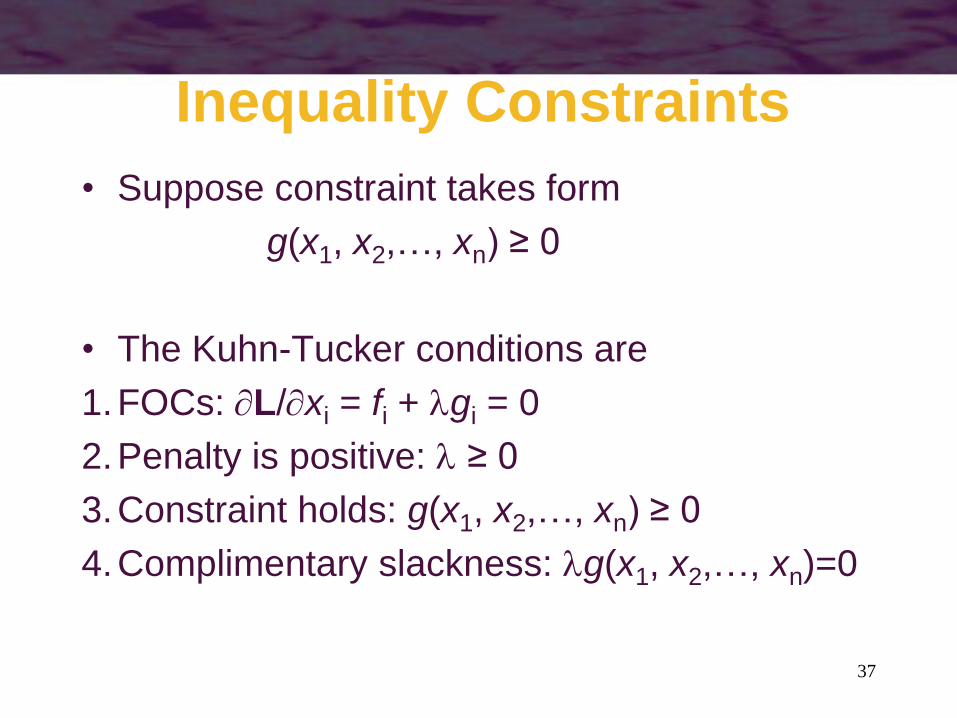
Inequality Constraints
• Suppose constraint takes form
g(x1, x2,…, xn) ≥ 0
• The Kuhn-Tucker conditions are
1.FOCs: L/xi = fi + gi = 0
2.Penalty is positive: ≥ 0
3.Constraint holds: g(x1, x2,…, xn) ≥ 0
4.Complimentary slackness: g(x1, x2,…, xn)=0

38
Example: Boundary Constraints
Suppose we maximise f(x) subject to x ≥ 0.
KT conditions imply that:
• If x*>0 then f’(x*)=0.
• If x*=0 then f’(x)≤0.

39
OTHER USEFUL RESULTS

40
Implicit Function Theorem
• Usually we write the dependent variable yas a function of one or more independent variable:
y = f(x)
• This is equivalent to:
y - f(x)=0
• Or more generally:
g(x,y)=0

41
Implicit Function Theorem
• Consider the implicit function:
g(x,y)=0
• The total differential is:
dg = gxdx+ gydy = 0
• If we solve for dy and divide by dx, we get the implicit derivate:
dy/dx=-gx/gy
• Providing gy≠0

42
Implicit Function Theorem
• The implicit function theorem establishes
the conditions under which we can derive
the implicit derivative of a variable
• In our course we will always assume that
this conditions are satisfied.
43
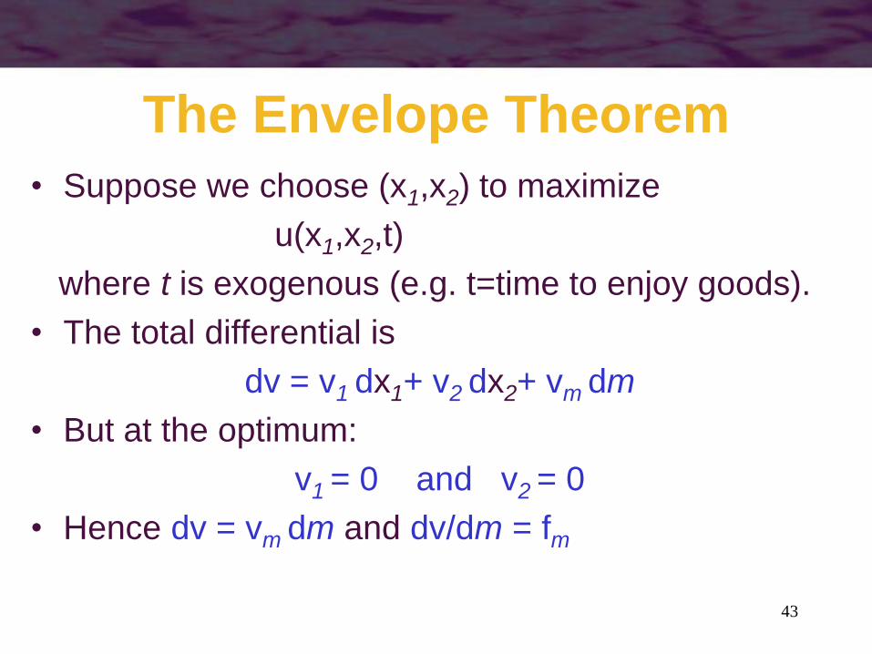
The Envelope Theorem
• Suppose we choose (x1,x2) to maximize
u(x1,x2,t)
where t is exogenous (e.g. t=time to enjoy goods).
• The total differential is
dv = v1 dx1+ v2 dx2+ vm dm
• But at the optimum:
v1 = 0 and v2 = 0
• Hence dv = vm dm and dv/dm = fm

44
The Envelope TheoremSuppose time t increases.
1.Changes goods consumer buys
– Spend more money on vacations.
2.Time also valuable in itself, holding consumption fixed.
• Envelope theorem says that only second effect
matters.
• First effect is second-order since consumption chosen optimally.

45
Homogeneous Functions
• A function f(x1,x2,…xn) is said to be
homogeneous of degree k if
f(tx1,tx2,…txn) = tk f(x1,x2,…xn)
– when a function is homogeneous of degree
one, a doubling of all of its arguments
doubles the value of the function itself
– when a function is homogeneous of degree
zero, a doubling of all of its arguments
leaves the value of the function unchanged

46
Homogeneous Functions
• If a function is homogeneous of degree
k, the partial derivatives of the function
will be homogeneous of degree k-1

47
Euler’s Theorem
• Euler’s theorem shows that, for
homogeneous functions, there is a special
relationship between the values of the
function and the values of its partial
derivatives.
• If a function f(x1,…,xn) is homogeneous of
degree k we have:
kf(x1,…,xn) = x1f1(x1,…,xn) + … + xnfn(x1,…,xn)

48
Euler’s Theorem
• If the function is homogeneous of degree
0:
0 = x1f1(x1,…,xn) + … + xnfn(x1,…,xn)
• If the function is homogeneous of degree
1:
f(x1,…,xn) = x1f1(x1,…,xn) + … + xnfn(x1,…,xn)

49
Duality
• Any constrained maximization problem
has associated with it a dual problem in
constrained minimization that focuses
attention on the constraints in the
original problem

50
Duality• Individuals maximize utility subject to a
budget constraint
– dual problem: individuals minimize the
expenditure needed to achieve a given level
of utility
• Firms maximize output for a given cost of
inputs purchased
– dual problem: firms minimize the cost of
inputs to produce a given level of output