Embed Size (px)
Citation preview

Microeconomic Principles (160)
Chapters 1 and 2
Economics is a social science that examines how a society (or individual) uses its limited resources to satisfy unlimited wants.
Resources or (factors of production) are land (natural resources), labor (human resources), and capital (durable man made inputs).
Scarcity => wants > resources (or ability to satisfy wants at zero price) Results in rationing and a positive price.
Scarcity => choices => trade-offs and competition
How do we make these choices (or ration the resources)?
1. force or violence2. politically (government decides) planning3. markets4. combination of the first three
Markets are institutional arrangements that enable buyers and sellers to get together in order to voluntarily (rather than a holdup that is involuntary exchange) exchange goods and services. Prices are determined in markets. Prices provide information (Car A cost $15,000 and car B costs $60,000, does this tell you anything?) and incentives that influence behavior. Moving resources efficiently to there highest valued use. Decentralized decisions rather than a central plan.
Problems with markets include monopoly, externalities, and public goods. All systems have equity issues. What is fair?
Private Property Rights are needed in order for markets to work. PPRs provide individuals the ability (“right”) to own and exercise control over scarce resources. Allows trading of these goods or resources. Can exclude others from using the resources. Owners capture any gains or loses. PPRs are enforce by the courts. You have recourse if PPRs are violated. Objective and fair court system needed. There are limits on PPRs (e.g. zoning and gun control). Contracts are a closely related idea that must also be enforced by the courts. Businesses are a series of contractual arrangements. PPRs can reduce violence. PPRs are the key to economic growth.
Trade-offs imply costs or opportunity costs. OCs are the benefits you give up of the highest valued alternative (something of value). The OC of holding cash is the interest rate. What is the OC of this class?
1
Positive analysis (or statements) deals with how the world actually works. Basic cause and effect. It is testable. Normative analysis (or statements) deal with how the world ought to be, subjective, or value judgements. How you would like things to be. It is not testable. Discuss wage differences.
Models capture simple key cause and effect relationships (e.g. driving directions). Amount of details are depend on the problem. Assumptions simplify the world or tell us what conditions need to hold in order to use the model.
MICROECONOMICS – the study of how household and firms make decisions and how they interact in markets.
MACROECONOMICS – the study of economy-wide phenomena, including inflation, unemployment, and economic growth. Economic growth and fluctuations.
PRODUCTION POSSIBILITIES FRONTIER
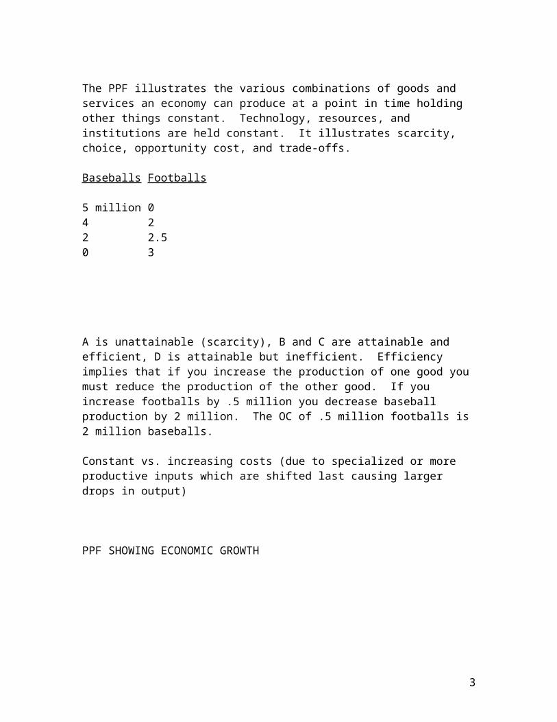
The PPF illustrates the various combinations of goods and services an economy can produce at a point in time holding other things constant. Technology, resources, and institutions are held constant. It illustrates scarcity, choice, opportunity cost, and trade-offs.
Baseballs Footballs
5 million 04 22 2.50 3
A is unattainable (scarcity), B and C are attainable and efficient, D is attainable but inefficient. Efficiency implies that if you increase the production of one good you must reduce the production of the other good. If you increase footballs by .5 million you decrease baseball production by 2 million. The OC of .5 million footballs is 2 million baseballs.
Constant vs. increasing costs (due to specialized or more productive inputs which are shifted last causing larger drops in output)
2
PPF SHOWING ECONOMIC GROWTH
Trade is like growth!
Circular Flow-shows how a simple economy (no explicit capital market, government, and the economy is closed) is organized. Households own the factors of production. There is a real flow and a dollar flow. Households supply labor and capital demanded by firms. Firms supply goods purchased by households. Household expenditures are revenue for firms. Wages and profits paid by firms are income for households.
Market for g &s
Firms HH
Market for factors
SUPPLY AND DEMAND (chapter 4)
Competitive short-run market
DEMAND – shows the various amounts of a good or service an individual is willing to purchase at all possible prices. Holding other things constant.
Held constant are:
3

1. Buyers income – an increase (decrease) in income that increases (decreases) demand is a normal good. It’s the reverse for an inferior (low quality) good.
2. Prices of related goods. Substitute goods – two goods that satisfy the same purpose. When the price of chicken goes up (reducing the quantity demanded of chicken), the demand for beef increases. Complementary goods – two goods that are consumed jointly. When the price of peanut butter goes up (reducing the quantity demanded of peanut butter), the demand for jelly decreases.
3. Tastes – if you like something more, demand increases. An apple a day keeps the doctor away, increases the demand for apples.
4. Expected prices – if you think the price of a TV will be lower next week, you will wait until next week to buy a new TV. Today’s demand for TVs decreases. Other examples are coffee and crude oil.
5. Other – weather, number of buyers, usefulness, etc.
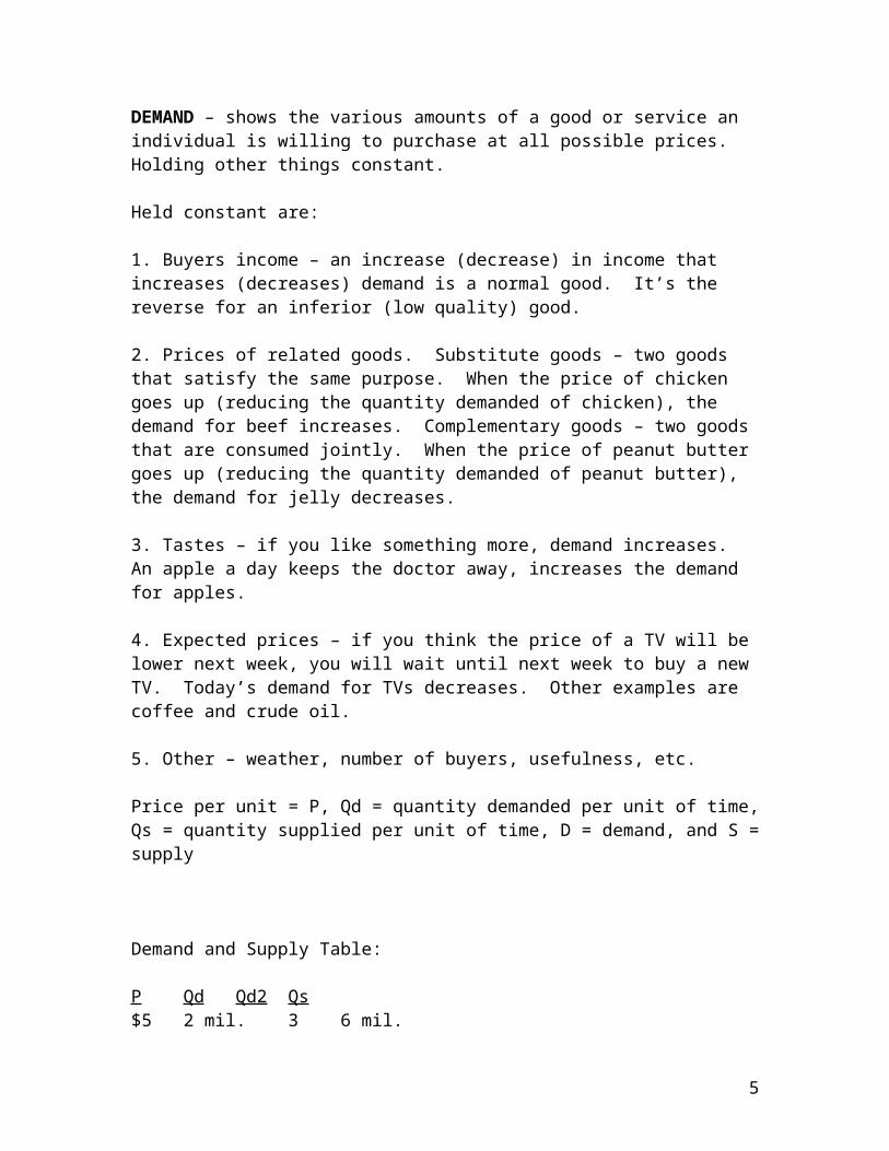
Price per unit = P, Qd = quantity demanded per unit of time, Qs = quantity supplied per unit of time, D = demand, and S = supply
Demand and Supply Table:
P Qd Qd2 Qs$5 2 mil. 3 6 mil.$4 3 4 5$3 4 5 4$2 5 6 3$1 6 7 2
Plot P and Qd
Law of demand – there is an inverse relationship between price and quantity demanded.
Why?
1. Diminishing subjective marginal valuation results in a decrease in willingness to pay.
2. Substitution effect – as the relative price increases (Px/Py, burgers/dogs = $4/$2 = 2 so burgers are twice as valuable as dogs or 2 dogs trades for 1 burger, $6/$2 = 3 now burgers are three times as valuable as dogs or 3D = 1B), you buy less of the relatively more expensive good. Income effect – as the price
4
increases, your real income (income/price, $100/$2 = 50 units, $100/$4 = 25 units) falls, reducing purchasing power and quantity demanded.
CHANGES IN DEMAND vs. CHANGES IN QUANTITY DEMANDED
MARKET DEMAND CURVE – is the horizontal sum of the individual demand curves.
SUPPLY – shows the various amounts of a good or service individuals are willing to sell at all possible prices. Holding other things constant.
Held constant are:
1. Input prices – higher input prices increase the cost of production, decreasing supply (shifts left).
2. Technology – an improvement in technology results in producing the same output at a lower cost or more output at the same price increase supply (shifts right).
3. Number of sellers – an increase in the number of sellers increases supply.
4. Expected prices – higher prices in the future reduces supply today.
5. Other – taxes and subsidies.
The supply curve shows the profit-maximizing behavior of sellers. It reflects the increasing marginal cost of production.
PLOT SUPPLY CURVE
5

CHANGES IN SUPPLY vs. CHANGES IN QUANTITY SUPPLIED
Market supply curve is the horizontal sum of individual supply curves.Comparative statics – start in equilibrium, change one factor at a time (shock the system), find new equilibrium, and compare equilibriums. Most of the models we will look at (in this class) are comparative static models.
Market equilibrium – price where Qs = Qd, the market clears, balance between buyers (who want a good deal, a low price) sellers (who want a good deal, a high price), market tends to adjust to the equilibrium.
Efficient allocation of resources that maximizes buyers and sellers gains from trade. Prices provide information and incentives that influence behavior.
EQUILIBRIUM
6

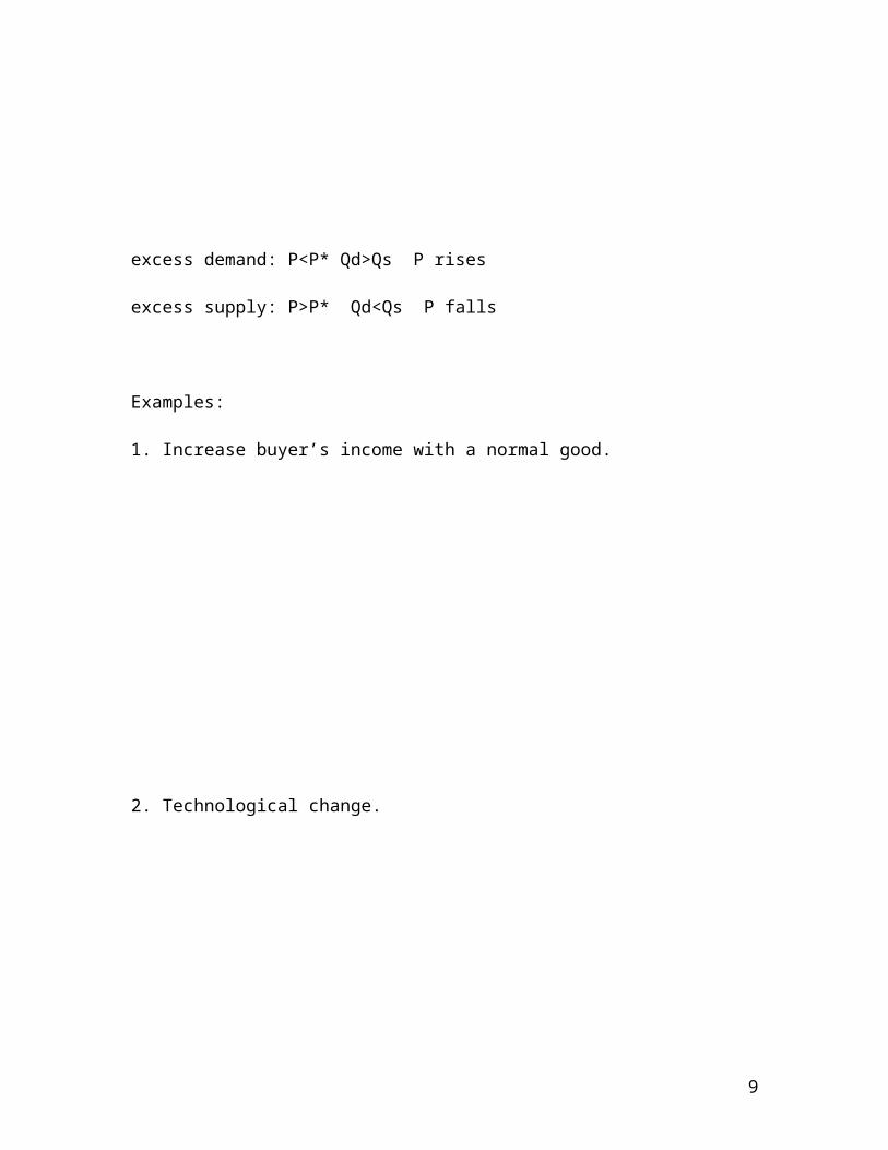
excess demand: P<P* Qd>Qs P rises
excess supply: P>P* Qd<Qs P falls
Examples:
1. Increase buyer’s income with a normal good.
2. Technological change.
3. 1 and 2 at the same time.
7

4. The impact of higher crude oil prices on gasoline and natural gas.
5. Beef and chicken example
Chapter 5
ELASTICITY
How can we measure the decline in quantity demanded when the price increases. We use price elasticity of demand (e). It measures the responsiveness of buyers to price changes. Since P and Q are measured in
8
different units, we use the percentage change which is unit free. We take the absolute value of e.
e= % change in Qd / % change in P
If % change in Qd > % change in P, then e>1 and demand is elastic.
If % change in Qd < % change in P, then e<1 and demand is inelastic
If % change in Qd = % change in P, then e=1 and demand is unit or unitary
Factor that influence e
1. The number of substitute goods (more substitutes, the more elastic2. The closeness of the substitute goods.3. The amount of time given to adjust to the price change.4. The definition of the market. The more narrowly defined is the market, the
more elastic demand (consumer has more good alteratives).5. Necessities tend to be inelastic and luxuries tend to be more elastic.
Estimates
Chapter 6
Price ceiling is a legal maximum price at which a good can be sold. Rent controls are an example of a price ceiling. It is binding when set below the equilibrium price. They result in a shortage in the market (Qd > Qs). The quality often declines, black markets develop, and non-price rationing. A wealth transfer from sellers to buyers.
Price floor is a legal minimum on the price at which a good can be sold. The minimum wage is an example of a price floor. They result in a surplus in the market (Qs > Qd). A wealth transfer from sellers to buyers.
9
TAXES
A specific tax is a per unit tax. So many dollars or cents per unit or a percentage of the price. An excise tax on gasoline or the payroll (Social Security and Medicare) tax are examples of specific taxes.
An important question, who pays the tax? Tax incidence measures the manner in which the burden of the tax is shared among participants. How much is passed on to the consumer.
I will look at the case when the tax is levied on the seller (as is usually the case). First think about the supply curve. Given the price, the quantity demanded is the profit maximizing amount. Or, given that quantity, the price is the minimum payment needed to induce the firm to sell that quantity.
STANDARD CASE:
The quantity decreases, buyers pay more, and sellers receive less. Note the tax revenue.
Tax incidence – the more inelastic demand (supply) the more of the tax is paid by the buyer (seller).
10

Chapters 7 and 8
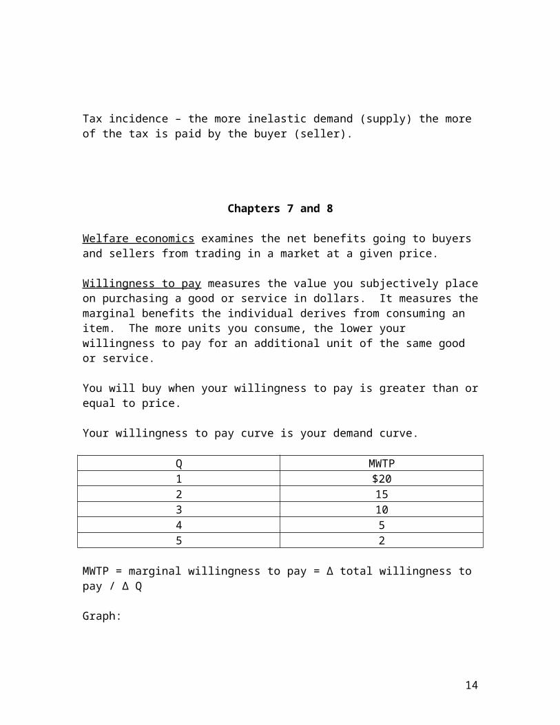
Welfare economics examines the net benefits going to buyers and sellers from trading in a market at a given price.
Willingness to pay measures the value you subjectively place on purchasing a good or service in dollars. It measures the marginal benefits the individual derives from consuming an item. The more units you consume, the lower your willingness to pay for an additional unit of the same good or service.
You will buy when your willingness to pay is greater than or equal to price.
Your willingness to pay curve is your demand curve.
Q MWTP1 $202 153 104 55 2
MWTP = marginal willingness to pay = ∆ total willingness to pay / ∆ Q
Graph:
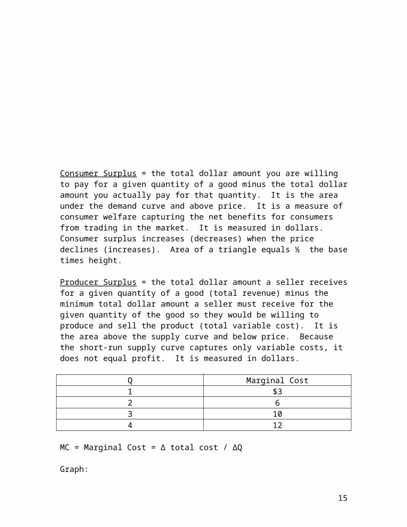
Consumer Surplus = the total dollar amount you are willing to pay for a given quantity of a good minus the total dollar amount you actually pay for that quantity. It is the area under the demand curve and above price. It is a measure of consumer welfare capturing the net benefits for consumers from trading in the market. It is measured in dollars. Consumer surplus increases (decreases) when the price declines (increases). Area of a triangle equals ½ the base times height.
11
Producer Surplus = the total dollar amount a seller receives for a given quantity of a good (total revenue) minus the minimum total dollar amount a seller must receive for the given quantity of the good so they would be willing to produce and sell the product (total variable cost). It is the area above the supply curve and below price. Because the short-run supply curve captures only variable costs, it does not equal profit. It is measured in dollars.
Q Marginal Cost1 $32 63 104 12
MC = Marginal Cost = ∆ total cost / ∆Q
Graph:
Total Surplus = CS + PS and is maximized at the competitive equilibrium. All mutually beneficial trades take place. It is an efficient outcome. Any output greater than or less than the competitive quantity reduces total surplus and welfare. It is inefficient.
12

Application: What is the deadweight loss of an excise tax imposed on the seller? The supply curve shifts up by the amount of the tax. The equilibrium quantity falls, the price paid by the buyer increases (generally less than the tax), and the net price received by the seller falls. Compare total surplus area before and after the tax? Notice it declines. There is also a deadweight loss from the tax. The estimated DWL of all U.S. taxes is between $1.15 to $1.50 per dollar of tax revenue raised by all levels of government.
Graph:
Chapters 3 and 9Globalization
Domestic markets for goods, services, and assets have increasingly become integrated into world markets. Developments outside the U.S. can have a large impact on the U.S. economy. It hasn’t always been this way. Between 1870 and 1914, there were large flows of goods and assets, comparable to today. However, between 1914 and 1945 there was reversal of these trends because of two world wars and the great depression. The flow of goods and assets have expanded since 1945.
This expansion has occurred for a number of reasons.
1. Lower transportation costs (steam vs. sail shipping in the 19th century, airplanes in the 20th century, and the internet today)
2. Containerization3. Reduced trade restrictions4. Increased incomes5. Vertical specialization (trade within firms may account for 1/3 of all trade)
INTERNATIONAL TRADE
13
Prior to the recent recession, world trade has been growing fast.
Quarterly world merchandise export developments, 2005-09(2005Q1=100, in current US dollars)
Source: World Trade Organization, downloaded 12.01.09.
Table I.8
Leading exporters and importers in world merchandise trade, 2008
(Billion dollars and percentage)
Rank Exporters Value Share
Annual percentage
change Rank Importers Value Share
Annual percentage
change
1 Germany 1461.9 9.1 11 1 United States 2169.5 13.2 72 China 1428.3 8.9 17 2 Germany 1203.8 7.3 143 United States 1287.4 8.0 12 3 China 1132.5 6.9 184 Japan 782.0 4.9 9 4 Japan 762.6 4.6 235 Netherlands 633.0 3.9 15 5 France 705.6 4.3 146 France 605.4 3.8 10 6 United Kingdom 632.0 3.8 17 Italy 538.0 3.3 8 7 Netherlands 573.2 3.5 168 Belgium 475.6 3.0 10 8 Italy 554.9 3.4 89 Russian Federation 471.6 2.9 33 9 Belgium 469.5 2.9 14
10 United Kingdom 458.6 2.9 4 10 Korea, Republic of 435.3 2.7 2211 Canada 456.5 2.8 9 11 Canada 418.3 2.5 712 Korea, Republic of 422.0 2.6 14 12 Spain 401.4 2.4 313 Hong Kong, China 370.2 2.3 6 13 Hong Kong, China 393.0 2.4 6
domestic exports 17.0 0.1 -6 retained imports 97.6 0.6 4 re-exports 353.3 2.2 7
14 Singapore 338.2 2.1 13 14 Mexico a 323.2 2.0 9 domestic exports 175.7 1.1 13 re-exports 162.5 1.0 13
14
15 Saudi Arabia 313.4 2.0 33 15 Singapore 319.8 1.947 22 retained imports 157.3 0.958 31
16 Mexico 291.7 1.8 7 16 India 293.4 1.8 3517 Spain 268.3 1.7 6 17 Russian Federation a 291.9 1.8 3118 Taipei, Chinese 255.6 1.6 4 18 Taipei, Chinese 240.4 1.5 1019 United Arab Emirates b 231.6 1.4 28 19 Poland 204.3 1.2 2320 Switzerland 200.3 1.2 16 20 Turkey 202.0 1.2 1921 Malaysia 199.5 1.2 13 21 Australia 200.3 1.2 2122 Brazil 197.9 1.2 23 22 Austria 183.4 1.1 1323 Australia 187.3 1.2 32 23 Switzerland 183.2 1.1 1424 Sweden 183.4 1.1 9 24 Brazil 182.4 1.1 4425 Austria 181.0 1.1 11 25 Thailand 178.7 1.1 2826 Thailand 177.8 1.1 17 26 Sweden 167.2 1.0 1027 India 177.5 1.1 21 27 United Arab Emirates b 165.6 1.0 2528 Norway 172.5 1.1 27 28 Malaysia 156.9 1.0 729 Poland 168.0 1.0 20 29 Czech Republic a 141.5 0.9 2030 Czech Republic 146.3 0.9 19 30 Indonesia 126.2 0.8 3631 Indonesia 139.3 0.9 18 31 Saudi Arabia 115.1 0.7 2832 Turkey 132.0 0.8 23 32 Denmark 110.8 0.7 1233 Ireland 124.1 0.8 2 33 Hungary 107.9 0.7 1334 Denmark 116.8 0.7 14 34 South Africa b 99.5 0.6 1235 Iran, Islamic Rep. of 113.4 0.7 28 35 Finland 91.8 0.6 1236 Hungary 107.7 0.7 13 36 Portugal 90.0 0.5 1537 Finland 96.5 0.6 7 37 Norway 89.3 0.5 1138 Bolivarian Rep. of Venezuela 93.5 0.6 35 38 Ukraine 85.5 0.5 4139 Kuwait 87.1 0.5 39 39 Ireland 83.2 0.5 -140 South Africa 80.8 0.5 16 40 Romania 82.7 0.5 1841 Nigeria 80.8 0.5 23 41 Viet Nam 80.4 0.5 2842 Algeria 79.3 0.5 32 42 Greece 79.0 0.5 443 Kazakhstan 71.2 0.4 49 43 Slovak Republic a 73.4 0.4 2244 Slovak Republic 71.0 0.4 22 44 Israel 67.7 0.4 1545 Argentina 70.0 0.4 26 45 Chile 61.9 0.4 3146 Angola b 67.1 0.4 51 46 Philippines 60.3 0.4 447 Ukraine 67.0 0.4 36 47 Argentina 57.4 0.4 2848 Chile 66.5 0.4 -2 48 Iran, Islamic Rep. of 57.4 0.4 2849 Qatar b 63.8 0.4 52 49 Bolivarian Rep. of Venezuela a, b 49.6 0.3 850 Libyan Arab Jamahiriya b 63.1 0.4 34 50 Egypt 47.5 0.3 28
Total of above c #### 92.5 - Total of above c #### 91.4 -
World c #### 100.0 15 World c #### 100.0 15
a Imports are valued f.o.b. b Secretariat estimates. c Includes significant re-exports or imports for re-export. Note: For annual data 1998-2008, see Appendix Tables A6 and A7.
Source: World Trade Organization, downloaded 12.01.09.
The U.S. is still a leading exporter (and importer) of merchandise, as well as services.
Leading exporters and importers in world trade in commercial services, 2008
(Billion dollars and percentage)
Rank Exporters Value Share
Annual percentage
change Rank Importers Value Share
Annual percentage
change
15

1 United States 521.4 13.8 10 1 United States 367.9 10.5 82 United Kingdom 283.0 7.5 1 2 Germany 283.0 8.1 113 Germany 241.6 6.4 11 3 United Kingdom 196.2 5.6 04 France 160.5 4.2 11 4 Japan 167.4 4.8 135 China 146.4 3.9 20 5 China 158.0 4.5 226 Japan 146.4 3.9 15 6 France 139.4 4.0 87 Spain 142.6 3.8 12 7 Italy 131.7 3.8 118 Italy 121.9 3.2 10 8 Ireland 106.2 3.0 129 India 102.6 2.7 17 9 Spain 104.3 3.0 9
10 Netherlands 101.6 2.7 8 10 Korea, Republic of 91.8 2.6 1211 Ireland 99.2 2.6 12 11 Netherlands 90.8 2.6 812 Hong Kong, China 92.3 2.4 9 12 Canada 86.6 2.5 613 Belgium 86.1 2.3 16 13 India 83.6 2.4 1814 Singapore 82.9 2.2 3 14 Belgium 81.9 2.3 1715 Switzerland 75.2 2.0 16 15 Singapore 78.9 2.3 616 Korea, Republic of 74.1 2.0 20 16 Russian Federation 74.6 2.1 2917 Denmark 72.0 1.9 17 17 Denmark 62.3 1.8 1618 Sweden 71.6 1.9 13 18 Sweden 54.3 1.6 1319 Luxembourg 68.9 1.8 5 19 Thailand 46.3 1.3 2120 Canada 64.8 1.7 2 20 Hong Kong, China 45.8 1.3 821 Austria 61.7 1.6 12 21 Australia 45.5 1.3 1822 Russian Federation 50.7 1.3 30 22 Brazil 44.4 1.3 2823 Greece 50.4 1.3 17 23 Norway 43.9 1.3 1324 Australia 45.6 1.2 15 24 United Arab Emirates 42.8 1.2 2825 Norway 45.6 1.2 13 25 Austria 42.6 1.2 926 Poland 35.3 0.9 23 26 Luxembourg 40.7 1.2 727 Turkey 34.5 0.9 22 27 Switzerland 36.6 1.0 1028 Taipei, Chinese 33.6 0.9 8 28 Saudi Arabia a 34.6 1.0 ...
29 Thailand 33.4 0.9 11 29 Taipei, Chinese 33.6 1.0 -230 Malaysia 29.3 0.8 4 30 Poland 29.9 0.9 2631 Brazil 28.8 0.8 27 31 Malaysia 29.1 0.8 532 Portugal 26.1 0.7 13 32 Indonesia a 27.9 0.8 ...
33 Egypt 24.7 0.7 26 33 Mexico 24.7 0.7 634 Finland 24.2 0.6 5 34 Greece 24.4 0.7 2335 Israel 23.8 0.6 13 35 Finland 23.1 0.7 536 Czech Republic 22.2 0.6 29 36 Israel 19.6 0.6 1137 Hungary 20.0 0.5 18 37 Hungary 18.5 0.5 2038 Lebanon 18.9 0.5 46 38 Czech Republic 17.3 0.5 2139 Mexico 18.5 0.5 5 39 South Africa 16.5 0.5 240 Macao, China 18.1 0.5 25 40 Portugal 16.5 0.5 17
Total of above #### 90.0 - Total of above #### 87.8 -
World #### 100.0 12 World #### 100.0 12
a Secretariat estimate.Note: Figures for a number of countries and territories have been estimated by the Secretariat. Annual percentage changes and rankings are affected by continuity breaks in the series for a large number of economies, and by limitations in cross-country comparability. See the Metadata. For annual data 1998-2008, see Appendix Tables A8 and A9.
Merchandise trade of the United States by origin and destination, 2008
(Billion dollars and percentage)
Exports Imports
Destination Value Share Share
Annual percentage
change
Origin Value Share
Annual percentage
change
2008 2000 2008 2007 2008 2008 2000 2008 2007 2008
16

Region Region
World #### 100.0 100.0 12 12 World #### 100.0 100.0 5North America 413.2 37.0 32.1 6 7 Asia 762.4 37.8 35.1 5Asia 329.4 27.6 25.6 11 8 North America 559.0 29.4 25.8 5Europe 311.1 23.6 24.2 16 14 Europe 409.6 20.3 18.9 6South and Central America 135.0 7.5 10.5 21 28 South and Central America 167.4 6.2 7.7 1Middle East 55.0 2.4 4.3 21 22 Africa 117.3 2.3 5.4 14Africa 28.8 1.4 2.2 28 20 Middle East 115.3 3.2 5.3 8CIS 13.8 0.4 1.1 49 32 CIS 38.5 0.8 1.8 5
Economy Economy
European Union (27) 271.8 21.6 21.1 15 11 European Union (27) 377.9 18.7 17.4 7Canada 260.9 22.6 20.3 8 5 China 356.6 8.5 16.4 11Mexico 151.2 14.3 11.7 2 11 Canada 339.1 18.5 15.6 3China 69.7 2.1 5.4 17 11 Mexico 218.6 10.9 10.1 6Japan 65.1 8.4 5.1 5 7 Japan 143.6 12.0 6.6 -2
Above 5 818.8 68.9 63.6 - - Above 5 #### 68.6 66.2 -Korea, Republic of 34.8 3.6 2.7 7 0 Saudi Arabia 57.0 1.2 2.6 12Brazil 32.3 2.0 2.5 28 34 Bolivarian Rep. of Venezuela 52.6 1.6 2.4 7Singapore 28.8 2.3 2.2 6 10 Korea, Republic of 49.8 3.3 2.3 4Taipei, Chinese 25.3 3.1 2.0 14 -4 Nigeria 39.2 0.9 1.8 17Australia 22.4 1.6 1.7 8 17 Taipei, Chinese 37.7 3.4 1.7 0Switzerland 22.0 1.3 1.7 18 29 Brazil 32.1 1.2 1.5 -3Hong Kong, China 21.6 1.9 1.7 13 8 Malaysia 31.6 2.1 1.5 -10India 17.7 0.5 1.4 55 18 Russian Federation 27.9 0.6 1.3 -2United Arab Emirates 15.7 0.3 1.2 -3 36 India 27.0 0.9 1.2 9Israel 14.5 1.0 1.1 19 11 Thailand 24.6 1.4 1.1 0Malaysia 13.0 1.4 1.0 -7 11 Iraq 23.1 0.5 1.1 -3Bolivarian Rep. of Venezuela 12.6 0.7 1.0 13 24 Israel 22.6 1.0 1.0 9Saudi Arabia 12.5 0.8 1.0 33 20 Algeria 20.0 0.2 0.9 15Chile 12.1 0.4 0.9 22 46 Angola 19.5 0.3 0.9 6Colombia 11.4 0.5 0.9 28 34 Switzerland 18.2 0.8 0.8 3Turkey 10.4 0.5 0.8 15 59 Indonesia 16.7 0.9 0.8 6Russian Federation 9.3 0.3 0.7 55 28 Singapore 16.2 1.6 0.7 3Thailand 9.1 0.9 0.7 4 7 Viet Nam 13.9 0.1 0.6 23Philippines 8.3 1.1 0.6 1 8 Colombia 13.8 0.6 0.6 2Argentina 7.5 0.6 0.6 23 29 Australia 10.9 0.5 0.5 5Dominican Republic 6.6 0.6 0.5 14 8 South Africa 10.1 0.3 0.5 20South Africa 6.5 0.4 0.5 24 18 Ecuador 9.5 0.2 0.4 -14Peru 6.2 0.2 0.5 41 50 Trinidad and Tobago 9.5 0.2 0.4 6Egypt 6.0 0.4 0.5 30 13 Philippines 9.1 1.1 0.4 -3Indonesia 5.9 0.3 0.5 38 40 Chile 9.0 0.3 0.4 -5Costa Rica 5.7 0.3 0.4 11 24 Norway 7.6 0.5 0.4 3Panama 4.9 0.2 0.4 38 32 Kuwait 7.4 0.2 0.3 3Honduras 4.8 0.3 0.4 21 9 Hong Kong, China 6.7 1.0 0.3 -12Guatemala 4.7 0.2 0.4 16 16 Argentina 6.2 0.3 0.3 13Nigeria 4.1 0.1 0.3 25 47 Peru 6.1 0.2 0.3 -11Ecuador 3.4 0.1 0.3 8 18 Congo 5.2 0.0 0.2 0Norway 3.4 0.2 0.3 27 11 Turkey 5.0 0.3 0.2 -15Qatar 3.1 0.0 0.2 108 11 Azerbaijan 4.5 0.0 0.2 162Netherlands Antilles 3.0 0.1 0.2 40 42 Libyan Arab Jamahiriya 4.4 ... 0.2 35Viet Nam 2.8 0.0 0.2 73 47 Honduras 4.2 0.3 0.2 5
Above 40 #### 97.1 95.6 - - Above 40 #### 96.5 96.6 -
Source: World Trade Organization, downloaded 12.01.09.
The bulk of U.S. trade is with North America, Asia, and Europe. All values are calculated in dollars using the average exchange rate over the period.
17

There are two kinds of trade, inter- and intra-industry trade. Inter-industry trade is between different industries. You export computers and import oil. Intra-industry trade represents trade within an industry. You export Bud and import Bass Ale.
Inter-industry trade is determined by comparative advantage, not absolute advantage. Comparative advantage implies you can produce something at a lower opportunity cost. The opportunity cost is the value of what you give up to produce something. Countries (and individuals) specialize in goods in which they have a comparative advantage. Absolute advantage measures the level of productivity. We can measure this in terms of the number of workers needed to produce one unit of the good.
Example:
Suppose we have productivity and population data for two countries, the Japan and Mexico. Both countries can produce mouthwash and garlic.
Productivity Data
Japan MexicoMouthwash 2 workers 8
Garlic 5 10
Japan is more productive than Mexico in both goods (it takes fewer workers to produce one unit of output). Is there any reason for Japan to trade with Mexico? Yes, specialize in the good with the comparative advantage. They have the comparative advantage in mouthwash. They can trade and import the other good. This will make them better off with a higher level of consumption.
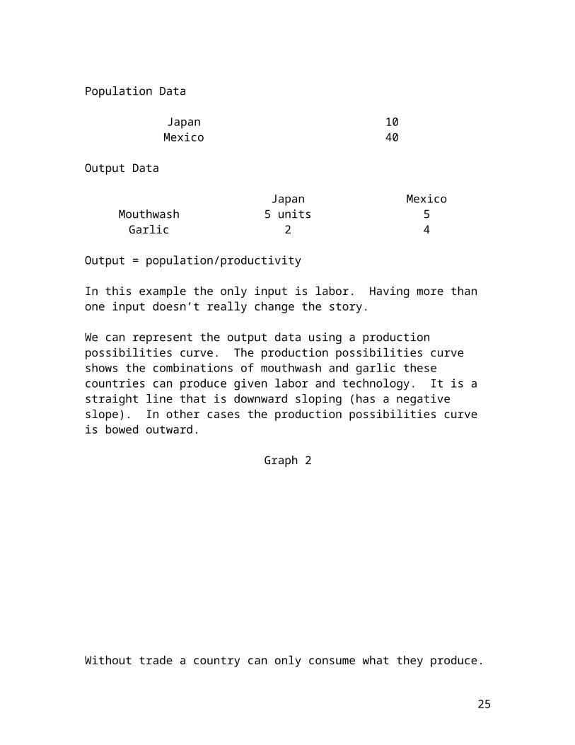
Population Data
Japan 10Mexico 40
Output Data
Japan MexicoMouthwash 5 units 5
Garlic 2 4
Output = population/productivity
In this example the only input is labor. Having more than one input doesn’t really change the story.
18

We can represent the output data using a production possibilities curve. The production possibilities curve shows the combinations of mouthwash and garlic these countries can produce given labor and technology. It is a straight line that is downward sloping (has a negative slope). In other cases the production possibilities curve is bowed outward.
Graph 2
Without trade a country can only consume what they produce.
Pre-trade Production and Consumption (This is one possibility.)
Japan MexicoMouthwash 2.5 units 1.25
Garlic 1 3
Compute opportunity cost to determine comparative advantage. We can do this by calculating the slope of the production possibilities curve. The slope of a straight line between two points equals the rise or change in the vertical distance between the two points (the change in mouthwash production) divided by the run or change in the horizontal distance between the two points (the change in garlic production). We will use the endpoints of the production possibilities curve. The slope can also be interpreted as the domestic (pre-trade) barter price. In this example, differences in technology or climate creates the comparative advantage.
Japan
∆ mouthwash / ∆ garlic = -5/2 = -2.5 Increase garlic by 2 causes mouthwash to decrease by 5 or ↑ garlic =1 → ↓ mouthwash by 2.5
∆ garlic / ∆ mouthwash = -2/5 = -.4 ↑ mouthwash= 5 → ↓ garlic = 2 or ↑ mouthwash=1 → ↓ garlic = .4
19

For Japan, the vertical intercept equals (0,5) and the horizontal intercept equals (2,0). The slope can be calculated using this information.
∆mouthwash/∆garlic = ∆y/∆x = 5 – 0/0 – 2 = 5/-2 = -2.5
Mexico
∆ mouthwash / ∆ garlic = -5/4 = -1.25 Increase garlic by 4 causes mouthwash to decrease by 5 or ↑ garlic =1 → ↓ mouthwash by 1.25
∆ garlic / ∆ mouthwash = -4/5 = -.8 ↑ mouthwash= 5→ ↓ garlic = 4 or ↑ mouthwash=1 → ↓ garlic = .8
For Mexico, the vertical intercept equals (0,5) and the horizontal intercept equals (4,0).
∆ mouthwash/∆garlic = 5 – 0/0 – 4 = 5/-4 = -1.25
Comparative Advantage
Comparative AdvantageJapan MouthwashMexico Garlic
Suppose the two countries decide to trade with each other based on comparative advantage. They would have to agree on a price. We can add a trading line with a slope equal to the international price (sometimes referred to as the terms of trade).
Mexico’s domestic price= 1.25 ≤ Price ≤ Japan’s domestic price = 2.5
Price = 2 → one pound of garlic would cost you 2 bottles of mouthwash
The closer the price is to Mexico’s domestic price, more of the gains go to Japan. So a decrease in the price of garlic (an improvement in Japan’s terms of trade) makes them better off. The reverse would be true for Mexico.
Mexico specializes in garlic production (output=4) and zero production of mouthwash. Mexico exports garlic and imports mouthwash. For every pound of garlic it exports it will receive or import two bottles of mouthwash. This is a good deal for Mexico. Without trade, Mexico gets 1.25 bottles of mouthwash for each pound of garlic it gives up. So long as the international price is greater than 1.25, they gain.
20

Japan specializes in mouthwash production (output=5) and zero production of garlic. Japan exports mouthwash and imports garlic. For every pound of garlic it imports it will give up two bottles of mouthwash. Without trade, each pound of garlic costs 2.5 bottles of mouthwash. Its cheaper to import it than produce it themselves.
Suppose they agree to trade 1 pound of garlic for 2 bottles of mouthwash.
Production with Specialization
Japan MexicoMouthwash 5 units 0
Garlic 0 4
Consumption after Trade
Japan MexicoMouthwash 3 units 2
Garlic 1 3
Consumption before Trade
Japan MexicoMouthwash 2.5 units 1.25
Garlic 1 3
Consumption Gains From Trade
Japan MexicoMouthwash .5 units .75
Garlic 0 0
Graph 3
They both consume more mouthwash and the same amount of garlic.
How large are these gains?
Japan when from a completely closed economy to a completely open economy in 1850. Real GDP rose by 8 percent. In 1807 President Jefferson imposed a trade embargo. Real GDP feel 5 percent in one year. Today, if all trade barriers in the world where eliminated, world GDP is estimated to increase by $2 trillion. U.S. GDP would increase by almost by half a trillion dollars. Studies also should countries grow faster when they open up to trade.
21

Heckscher-Ohlin Model of Comparative Advantage: Assuming technology and tastes are the same, a country will have a comparative advantage and export goods that are intensive in the country’s abundant factor of production.
Compare Factor Endowments
(Skilled Labor / Unskilled Labor)US > (Skilled Labor / Unskilled Labor)VIETNAM
The U.S. will export goods than are skill intensive and import goods intensive in unskilled labor from Vietnam. Since the U.S. has a lot of skilled labor relative to unskilled labor, goods that use a lot of skilled labor should be cheaper to produce it the U.S. We tend to see this. So this is another reason why a country can have a comparative advantage in addition to technology differences. Today, technology is diffused around the globe quickly.
This approach is useful for understand the potential impact of trade on wages.
Stolper-Samuelson Theorem: Trade causes the real income of the owners of the adundant factor (skilled labor in the U.S.) to increase and decreases the real income of the scare factor, other things constant. Key point, the country as a whole is better off but some individuals can be harmed. That is why we set up programs that help displaced workers. Ignoring productivity growth and holding labor supply constant, the demand for skilled labor in the U.S. increases raising the wages of skilled labor. The demand for unskilled labor declines causing wages of the less skilled workers to decline (or not grow).
Graph 4 – Labor Market Effects
What is the impact on aggregate employment? Over the last 20 years employment increased 35 percent while imports increased 370 percent. The impact of trade on employment and wages is modest. Technological change has had a far bigger impact on wage inequality.
Intra-Industry Trade
This represents trade within the same industry. The U.S. exports and imports golf clubs. This occurs in markets where firms differentiate their product and experience declining average costs as production expands. International trade expands the size of their market causing average costs decline lowering prices. Lower prices and greater variety increase consumer welfare. The value to consumers from greater variety is estimated to equal $300 billion per year.
22

Trade Policy
While the U.S. has reduced trade restrictions, the tariffs that remain in place are at relatively low levels. Tariffs are a tax on imports. What is the impact(s) of an import tariff? We can analyze this using supply and demand. To understand the overall impact on consumers, producers, and the economy, we can use consumer and producer surplus.
Consumer surplus = the total dollar amount you are willing to pay for a given quantity of a good minus the total dollar amount you actually pay for the given quantity of the good. It is the area under the demand curve and above price. It is a measure of consumer welfare capturing the net benefits for consumers from trading in a market. It is measured in dollars.
Graph 5 – Consumer Surplus
Producer surplus = the total dollar amount a seller receives for a given quantity of a good (total revenue) minus the minimum total dollar amount a seller must receive for the given quantity of the good so they would be willing to produce and sell the product (total variable cost). It is the area above the supply curve and below price. Because the supply curve captures only variable costs, it does not equal profit. It is measured in dollars.
Graph 6 – Producer Surplus
Graph 7 - Total Surplus
P = the domestic price of the good. Pw = the world price of the good,
When Pw < P a country will import the good or service.
When Pw > P a country will export the good or service.
Graph 8 – Import TariffFree Trade:
Consumer surplus = a+b+c+d+e+f
Producer surplus = g
Trade with Tariff:
Consumer surplus = a+b
Producer surplus = g+c
23
Net reduction in consumer surplus = a+b+c+d+e+f – a+b = c+d+e+f
Net increase in producer surplus = g+c – g = c
e = tariff revenue (This area is a quota rent under an import quota. It is captured by the government if licenses are auction off. If the government gives the licenses to domestic importers (foreign exporters), importers (foreign exporters) capture the area.
f = lost consumer surplus, Qd is lower because of the higher price.
d = higher cost associated with producing the additional output rather than importing the good.
f + d = deadweight loss of the tariff or net loss to society.
U.S. Sugar Quota:
c = $1.2 billion per year, d = $300 million per year f = $50 million per year, and c= $100 million per year (foreign sugar suppliers some of whom are U.S. growers. This works out to approximately $500,000 per farmer and $5 per consumer. Farmers lobby and make campaign contributions to both parties while consumers do not. Farmers are a small homogeneous group the is geographically concentrated so organization costs are low. This is not true for consumers. The higher cost of sugar has caused candy companies to move off shore.
Estimates of the increased cost to consumers per job saved averaged $168,177 per year over 21 sectors in the U.S. using data from 1990. This is three times the average wage in manufacturing.
Cost to Consumers per Job Saved per Year by the Import Restriction
Textiles $202,061Sugar $600,177
Lumber $758,678Machine Tools $348,329
Costume Jewelry $96,532Benzenoid Chemicals $1,000,000
Apparel $138,666
Source: Hufbauer and Elliott, 1994, Measuring the Costs of Protection in the U.S.
Regional Trade Agreements
24
These are agreements between a group of countries to provide preferential access to their economies to the other countries that are part of the agreement. These countries cannot impose higher restrictions on non-members.
Regional Trade Agreements
Free-Trade Area
Customs Union
Common Market
Economic Union
No internal trade barriers
Yes Yes Yes Yes
Individual external trade
barriers
Yes No No No
Common external trade
barriers
No Yes Yes Yes
Free flow of factors
internally
No No Yes Yes
Common policies
No No No Yes
NAFTA is a free-trade area between the U.S., Canada, and Mexico. A monetary union has one currency. Europe and the U.S. have common currencies.
These kinds of agreements cause trade creation and trade diversion.
Trade Creation: Switching imports from a higher cost country to a lower cost country that is a member of the agreement. This is your standard gains from trade when you remove a tariff. This increases country welfare.
Trade Diversion: Switching imports from the lowest cost country that is not a member (that still has a tariff on its product) to a higher cost member country(that no longer has a tariff on its product). This lowers country welfare.
So long as trade creation is greater than trade diversion, there is a net improvement in country welfare.
These are notes for chapters 13, 14, 15, and 16.
Costs of Production – Chapter 13
25

The basic building block for understanding the costs of production is the firm’s production function. The production function shows the relationship between inputs and output.
Q = f (K, L)
Where Q= firm output, K = physical capital, L = Labor, and f ( ) = function notation.
In the short run, one input is held constant. Once the factory is built, capital is constant or fixed input. Labor is the variable input. It could be reversed with labor fixed and capital variable. In the long run, all inputs are variable.
If capital is fixed and technology is held constant, then we can define the marginal product of labor (MPL) as:
MPL = ∆Q / ∆L
MPL measures the extra output that results from increasing the labor input (usually by 1).
Assuming labor and technology constant, the marginal product of capital (MPK) can be defined as:
MPK = ∆Q / ∆K
Put into words what the equation means.
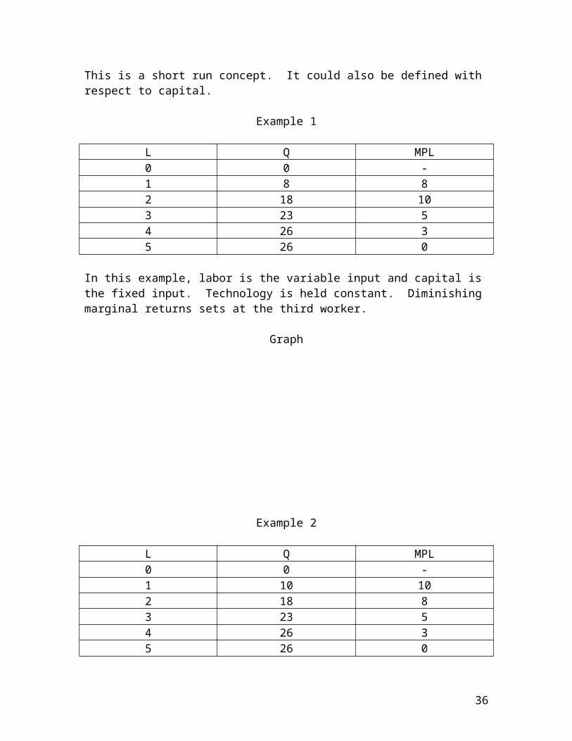
Suppose capital and technology is held constant, Diminishing Marginal Returns occurs when the MPL starts to decline. This is a short run concept. It could also be defined with respect to capital.
Example 1
L Q MPL0 0 -1 8 82 18 103 23 54 26 35 26 0
In this example, labor is the variable input and capital is the fixed input. Technology is held constant. Diminishing marginal returns sets at the third worker.
26

Graph
Example 2
L Q MPL0 0 -1 10 102 18 83 23 54 26 35 26 0
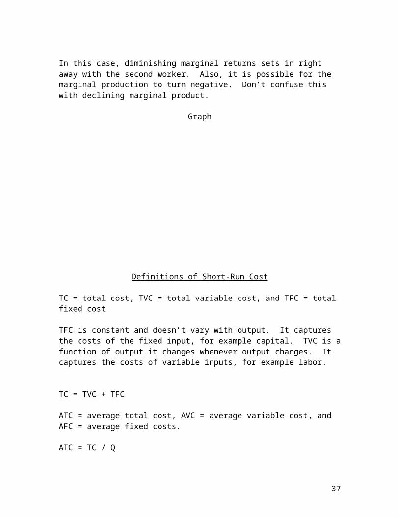
In this case, diminishing marginal returns sets in right away with the second worker. Also, it is possible for the marginal production to turn negative. Don’t confuse this with declining marginal product.
Graph
Definitions of Short-Run Cost
TC = total cost, TVC = total variable cost, and TFC = total fixed cost
27

TFC is constant and doesn’t vary with output. It captures the costs of the fixed input, for example capital. TVC is a function of output it changes whenever output changes. It captures the costs of variable inputs, for example labor.
TC = TVC + TFC
ATC = average total cost, AVC = average variable cost, and AFC = average fixed costs.
ATC = TC / Q
AVC = TVC / Q
AFC = TFC / Q
AFC will decline as output increases because TFC is constant. ATC and AVC will generally have a “U” shape curves.
ATC = AVC + AFC => AFC = ATC - AVC
MC = marginal cost = ∆TC / ∆Q = ∆TVC / ∆Q
Marginal cost measures the change in TC (or TVC) that results from a unit change in output. It is the incremental cost of production.
Example of Typical Cost Curves
28

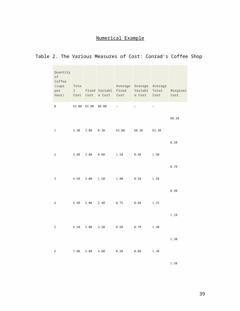
Numerical Example
Table 2. The Various Measures of Cost: Conrad's Coffee Shop
Quantity of Coffee (cups per hour)
Total Cost
Fixed Cost
Variable Cost
Average Fixed Cost
Average Variable Cost
Average Total Cost
Marginal Cost
0 $3.00 $3.00 $0.00 – – –
$0.30
1 3.30 3.00 0.30 $3.00 $0.30 $3.30
0.50
2 3.80 3.00 0.80 1.50 0.40 1.90
29

0.70
3 4.50 3.00 1.50 1.00 0.50 1.50
0.90
4 5.40 3.00 2.40 0.75 0.60 1.35
1.10
5 6.50 3.00 3.50 0.60 0.70 1.30
1.30
6 7.80 3.00 4.80 0.50 0.80 1.30
1.50
7 9.30 3.00 6.30 0.43 0.90 1.33
1.70
8 11.00 3.00 8.00 0.38 1.00 1.38
1.90
9 12.90 3.00 9.90 0.33 1.10 1.43
2.10
10 15.00 3.00 12.00 0.30 1.20 1.50
30

The Relationship between TC and MC
MC and Diminishing Marginal Returns
MC = ∆TC / ∆Q = ∆TVC / ∆Q = W∆L / ∆Q = W / MPL
Where ∆L / ∆Q = 1/MPL , ∆TVC = W∆L, and W = wage
MC = W / MPL
This tells us there is an inverse relationship between MC and MPL holding W constant. When diminishing marginal returns sets in, the MPL starts to decline so MC must rise. Each time the firm expands output by one unit, it must use increasing amounts (more than the previous increase) so marginal cost must rise.
An increase in W, other things constant shifts the MC curve up.
31

The Average – Marginal Relationship
MC > ATC => ATC increasesMC < ATC => ATC decreasesMC = ATC => ATC at its minimum
Long-Run Costs
All inputs are variable in the long run. The firm now decides which combination of capital and labor allows you to produce the output at lowest cost.
LRATC = LRTC / Q
It is “U” shaped. Why?
The firm increases ALL inputs by the same proportion.
Economies of scale: The increase in output is more than proportional to an increase in all inputs. You double all inputs and output more than doubles. It is the result of specialization. LRATC declines. Or for technical reasons such as, when you double the circumference of a pipeline, volume increases more than double.
Constant returns to scale: The increase in output is proportional to the increase in all inputs. You double all inputs and output doubles. LRATC is flat.
Diseconomies of scale: The increase in output is less than proportional to the increase in all inputs. You double all inputs and output increases less than double. It is associated with managing large organizations. There are coordination problems with running large firms.
32

Numerical Example
LRATC = LRTC / Q = $1000 / 100 = $10
Now suppose you double all inputs. Under CRS, LRTC doubles and so does Q.
LRATC = $2000 / 200 = $10
LRATC is constant.
Under EOS LRATC = $2000 / 300 = $6.67
LRATC is declining.
Under DOS LRATC = $2000 / 150 = $13.33
LRATC is increasing.
Relationship Between ATC and LRATC
Because you have greater input flexibility in the long run, LRATC will tend to be less than ATC.
33

Impact on Market Structure
Industries with extensive EOS will tend to have fewer big firms for a given level of demand. Industries with limited EOS will tend to have a large number of small firms for a given level of demand.
Minimum Efficient Scale is the lowest level of output where LRATC is at its lowest value.
Economic Profit = Total Revenue – Total Cost
TR = P x Q
TC = Explicit Costs + Implicit Costs
Total cost includes explicit cost where there are observable dollar outlays by the business on inputs. It also includes any implicit or opportunity costs such as the value of the owner’s alternative use of time or alternative returns on investment.
34

Economic and accounting profits differ because economics focuses on why resources are use in a particular manner. Consider an owner operated business. The owner’s income is the profits of the business. Explicit costs include wages, rent, inventory, and taxes. The implicit cost equals what the owner would earn working for someone else. Assume the numbers provided below have been stable for some time and are expected to remain that way.
A B CTR $100,000 $100,000 $100,000
Explicit Costs $60,000 $60,000 $60,000Accounting Profit $40,000 $40,000 $40,000
Implicit Costs $30,000 $45,000 $40,000Economic Profit +$10,000 -$5,000 0
In situation A, the owner earns positive economic profits and cannot do better elsewhere. The business continues to operate. In situation B, the owner earns negative economic profits and can do better elsewhere. The business is closed. In situation C, the owner earns zero economic profit. The owner does the same either working or running the business. The business continues to operate. Zero economic profit is called normal economic profit. In this case the owner’s income will be $40,000 which equals the accounting profit. Competition drives economic profit toward zero.
The goal of the firm is to maximize total economic profit.
Competition – Chapter 14
Industry Structure: The degree of competition varies between industries.
1. Competition2. Monopoly3. Monopolistic Competition4. Oligopoly
Competition – In the short run
Characteristics
1. Many buyers and sellers – each firm is a price taker. This means they have no influence over the price the good or service sells for in the market. They have no market power. Commodity prices are determined by world supply and demand. As an individual business, you take the price as given and determine the profit maximizing output to produce.
35
2. Products are homogeneous – they are perfect substitutes for each other. There is no product differentiation.
3. Easy entry and exit – there are no restrictions (barriers) on entering or exiting the industry.
Marginal revenue = MR = ∆TR / ∆Q
For the representative firm in a competitive industry, MR = P, the firm’s MR curve will also serve as the firms demand curve.
Average Revenue = AR = TR/Q = (P x Q) / Q = P
Graph
Table 1. Total, Average, and Marginal Revenue for a Competitive Firm
Quantity (Q)
Price (P)
Total Revenue (TR = P × Q)
Average Revenue (AR = TR / Q)
Marginal Revenue (MR =ΔTR / ΔQ)
1 gallon $6 $6 $6
$6
2 6 12 6
6
3 6 18 6
6
36
4 6 24 6
6
5 6 30 6
6
6 6 36 6
6
7 6 42 6
6
8 6 48 6
Profit Maximization
Firms maximize total economic profit (TR – TC) when output is adjusted to a level where marginal cost equals marginal revenue.
MC = MR = P
Table 2. Profit Maximization: A Numerical Example
Quantity (Q)
Total Revenue (TR)
Total Cost (TC)
Profit (TR – TC)
Marginal Revenue (MR = ΔTR / ΔQ)
Marginal Cost (MC = ΔTC / ΔQ)
Change in Profit (MR – MC)
0 gallons $0 $3 –$3
$6 $2 $4
1 6 5 1
37

6 3 3
2 12 8 4
6 4 2
3 18 12 6
6 5 1
4 24 17 7
6 6 0
5 30 23 7
6 7 –1
6 36 30 6
6 8 –2
7 42 38 4
6 9 –3
8 48 47 1
Graph of Industry and Firm
38
Graph of a competitive firm maximizing profits
Suppose MR = $10 and MC = $15. Reducing output will increase total profits because ∆Profits = MR – MC = -$10 – (-$15) = +$5.
Suppose MR = $10 AND MC = $5. Increasing output will increase total profits because ∆Profits = MR – MC = $10 - $5 = +$5.
Calculating Total Profits (Numerically and Graphically)
Profits = TR – TC, where TR = P x Q and TC = ATC x Q
Profits = (P – ATC) x Q
Example 1
MC = MR = P = $20, ATC = $15, Q = 10
TR = $20 x 10 = $200TC = $15 x 10 = $150Profit = $50
Or
($20 - $15) X 10 = $50
39

Graph
Example 2
MC = MR = P = $15, ATC = $20, AVC = $10, Q=10
TR = $15 x 10 = $150TC = $20 x 10 = $200Profit = $150 - $200 = -$50
The business is operating at a loss in short run. What should the business do? You short-run options are produce at a loss or temporarily shutdown. How do you decide? If you produce you lose $50. If you shutdown your loss will equal TFC. TFC = AFC x Q. AFC = ATC – AVC
TFC = ($20 - $10) x 10 = $10 x 10 = $100. The business would lose more ($100) if they shutdown. Profit maximization when you are losing money is to minimize your losses. This business will continue to produce.
Graph
40
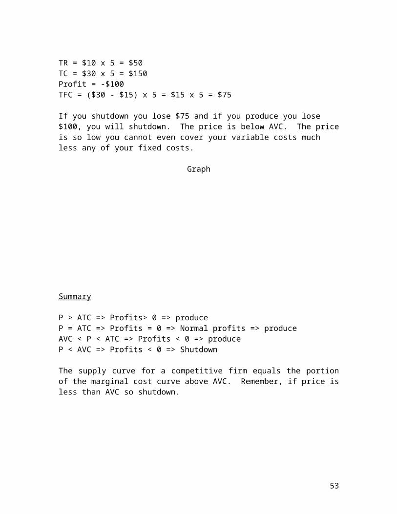
Example 3
MC = MR = P = $10, ATC = $30, AVC = $15, Q = 5
TR = $10 x 5 = $50TC = $30 x 5 = $150Profit = -$100TFC = ($30 - $15) x 5 = $15 x 5 = $75
If you shutdown you lose $75 and if you produce you lose $100, you will shutdown. The price is below AVC. The price is so low you cannot even cover your variable costs much less any of your fixed costs.
Graph
Summary
P > ATC => Profits> 0 => produceP = ATC => Profits = 0 => Normal profits => produceAVC < P < ATC => Profits < 0 => produceP < AVC => Profits < 0 => Shutdown
The supply curve for a competitive firm equals the portion of the marginal cost curve above AVC. Remember, if price is less than AVC so shutdown.
41
Any change in wages or the MPL will shift the firm’s marginal cost curve and supply curve.
Recall: MC = W / MPL
Graph – higher oil prices
Graph – higher labor productivity
Competition in the Long Run
Important Idea: What is the significance of no barriers to entry?
P > LRATC => Profit > 0 => entry (more firms) => P↓ => Profits↓ and entry stops
P < LRATC => Profits < 0 => exit (less firms) => P↑ => Profits↑ and exit stops
P = LRATC => Profits = 0 => Normal Profits => No incentive to exit or enter
Long – Run Equilibrium
42
Competition leads to the following conditions hold in long – run equilibrium.
1. Profits are maximized MC = MR2. Profit = 0 or firms earn a normal profit3. Firms adjust the scale of operation so that LRATC and ATC are at a
minimum.
Graph
Long –run Industry Supply Curves
Constant – Cost Industry: As the industry expands (or gets smaller) factor prices remain constant resulting in no change in costs. This is fairly common for retail stores. We assume factor supply does not change.
Increasing – Cost Industry: As the industry expands (or gets smaller) factor prices increase (decrease) causing costs to rise (decrease). The aerospace and computer industries fit this category.
43
Decreasing – Cost Industry: As the industry expands (or gets smaller) factor prices decline (increase) causing costs to fall (increase). Suppliers locate near producers. Do not confuse this with lower cost because of technological change.
Deriving the long – run Industry Supply Curve (Constant – Cost Industry)
Assume the industry starts in long – run equilibrium (Profits = 0) and industry demand increases. The demand curve shifts right and price and quantity increase. We adjust along the short – run supply curve. Profits are now positive so entry occurs causing the short – run supply curve to shift to the right. This causes price and profits to fall. Entry stops when the price falls enough so that profits return to zero. Price returns to the initial level in a constant – cost industry.
In an increasing – cost industry, the adjustment is the same except costs would also rise so the new long – run equilibrium price would be higher than before, reflecting the higher costs.
In a decreasing – cost industry, the adjustment is the same except costs would also fall so the new long – run equilibrium price would be lower than before reflecting the lower costs.
44

CHAPTER 15 – MONOPOLY
A monopoly firm is an industry where there is only one seller. There are no close substitutes for the good or service being sold. They are a price maker and have market power. Market power occurs when the individual firm can alter the price when it changes output. Monopolies restrict trade causing the price to rise above the competitive price. Examples include the power and electric utilities. Cable TV now faces competition from dish TV. A drug company that creates a new drug that is patented has a monopoly (On average they spend approximately $800 million per drug and only 3 of 10 turn out to be profitable).
Sources of Monopoly Power:
1. Barriers to entry: These are costs that the entrant pays that existing firms do not pay. You have to get government approval to enter the market. Examples include patents (good for 20 years in the U.S.), tariffs, and licenses.
2. Economies of scale: declining LRATC can give the first firm to take advantage of the EOS a cost advantage that deters entry. This is called a natural monopoly.
3. Control of a key input: An example of this is Debeers diamonds.
OPEC is an example of a cartel. A cartel is a group of producers that act like a monopoly. Microsoft certainly has market power with its dominant operating system. It also has economies of scale and network effects (the value to the consumer depends on how many other people buy or use the good). Finally, product differentiation can give a firm market power. We will discuss this in monopolistic competition.
The demand curve for a monopolist is the negatively sloped market demand curve. Recall the upper half of the demand curve is elastic and the lower half is inelastic.
Demand, Total Revenue, and Marginal Revenue
MR = ∆TR / ∆Q and TR = P x Q
45

Elastic Demand: ↓P => ↑Q => ↑TR
Inelastic Demand: ↓P => ↑Q => ↓TR
Starting at the top of the demand curve where Q = 0 so TR = 0, we lower P and Q increases. Since demand is elastic, total revenue increases. When we move into the inelastic portion of the demand curve and continue to lower price, total revenue decrease. Total revenue equals zero when price equals zero.
Since MR is the slope of the TR curve, we can see it is positive and falling in the elastic portion of the demand curve and negative and falling in the inelastic portion of the demand curve. MR equals zero at the unit elastic point where TR is at a maximum.
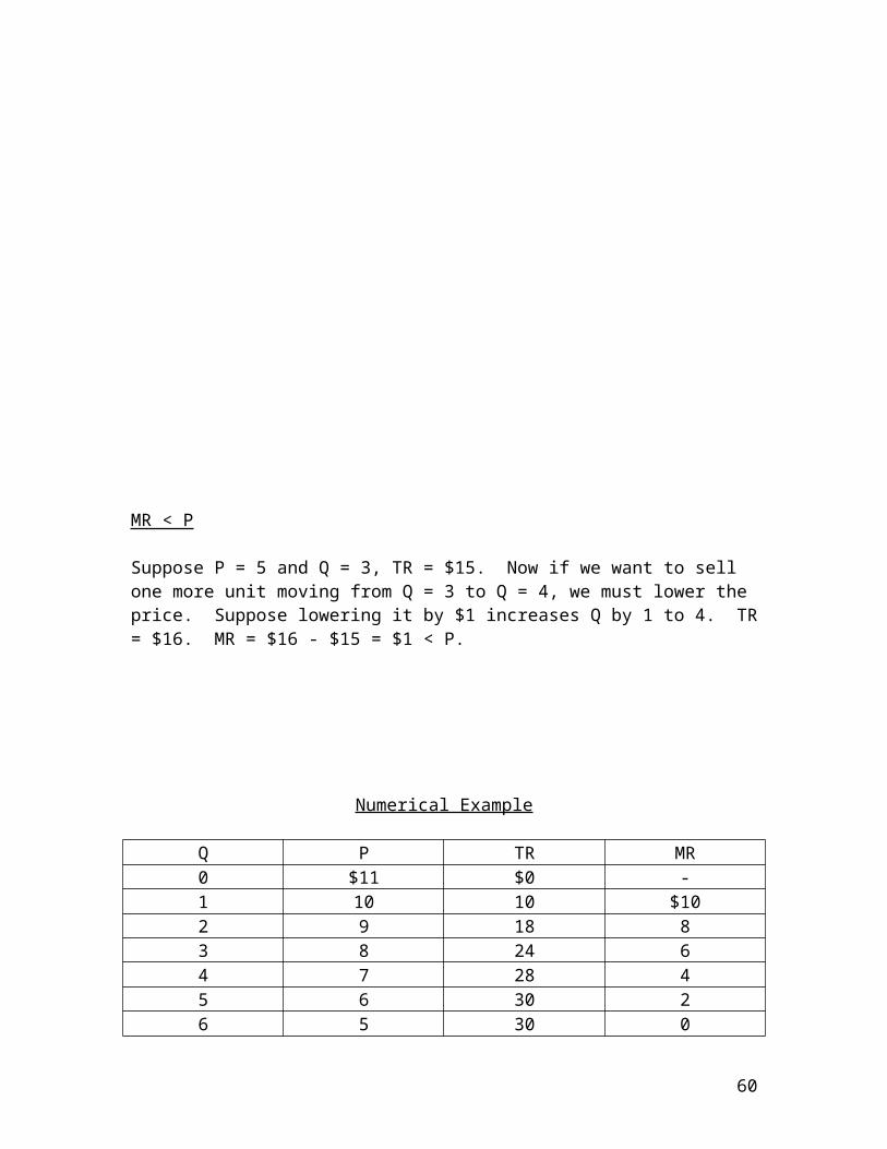
MR < P
Suppose P = 5 and Q = 3, TR = $15. Now if we want to sell one more unit moving from Q = 3 to Q = 4, we must lower the price. Suppose lowering it by $1 increases Q by 1 to 4. TR = $16. MR = $16 - $15 = $1 < P.
46

Numerical Example
Q P TR MR0 $11 $0 -1 10 10 $102 9 18 83 8 24 64 7 28 45 6 30 26 5 30 07 4 28 -28 3 24 -4
Monopoly Equilibrium
The monopoly produces an output where MC = MR < P and maximizes its total profits. Total profits equals TR minus TC or (P – ATC) x Q.
Deadweight Loss of Monopoly
When we compare monopoly with competition we notice some differences.
1. Monopoly output is less than the competitive output.
2. Monopoly price is higher than the competitive price.
1 and 2 imply the monopolist restricts trade resulting in lost consumer and producer surplus. We call this the deadweight loss of monopoly. The triangle
47

represents the deadweight loss of monopoly. It is equal to 1 – 3 percent of GDP. The cost to society is higher because firms waste time lobbying government for monopoly power rather than producing goods and services.
Key Antitrust Laws
Sherman Act of 1890:
This law prohibited “restraint of trade” so it outlawed monopoly, collusion, and price fixing (cartels). It did not address the question of mergers.
Clayton Act of 1914:
This law made mergers illegal if they “substantially” reduce competition. What does substantially mean? Today we have measures and guidelines on competition before and after a proposed merger to help judge the impact on competition.
We are concerned about mergers if they reduce competition because this would lower consumer welfare. However, mergers can increase efficiency which increases consumer welfare. This is what antitrust cases have to decide. Which factor is more important.
48

Natural Monopoly
This occurs went there are significant economies of scale. Utilities and pipelines are good examples. We allow these monopolies to exist to take advantage of the lower costs to consumers but regulate them so the do not restrict output, harming consumers.
Monopoly Pricing: MC = MR < P and there is a deadweight loss.
Regulate:
1. Marginal – Cost Pricing: produce the output where P = MC like in competition. The problem is that this results in negative profits. The government must subsidize or own it. This is costly to the taxpayer.
2. Average – Cost Pricing: produce the output where P = ATC and profits are zero. In this case, there is little incentive to innovate or lower costs. It is easy to carry out this form of regulation. It was used in the past in the airline industry.
3. Block Pricing: charge different prices to different groups of customers. This results in a higher output and normal profits.
49

Price Discrimination
There are a number of reasons why prices for the same good or service differ:
1. Cost differences: it can be more costly to run a business one location because of crime.
2. Transaction and information costs: a transaction that is more difficult to carry out (higher transaction costs) might have to charge a lower price. Consumers may not know the lowest price in an area because of imperfect information.
3. Price discrimination: there are many types of price discrimination. We can define one type as charging different prices when the costs are the same. Examples include Disneyland, airlines, movies, coupons, and financial aid.
Perfect price discrimination amounts to the business pricing to capture your consumer surplus. If you know a person’s demand curve, then you can charge what they are willing to pay for each unit of the good. Amazon has done this type of pricing.
Conditions:
1. The firm must have market power.
2. The firm must be able to separate customers and markets. This can be done using demographics, income, or location.
3. Once separated, there can be little resale between markets.
4. Different price elasticity of demand.
Profit Maximizing Rule with Price Discrimination:
MC = MR1 = MR2
Why equalize the marginal revenues between market 1 and market 2?
Profit = TR – TC and suppose the total amount sold in two markets is held constant. This means TC is constant. Now we focus on the impact of selling different quantities in the two markets on TR. If we can increase TR with TC constant we increased profits. This is the reason to price discriminate.
50

If MR1 < MR2, then by selling more in market 2 and less in market 1, holding total combined output constant (so TC is constant) increases TR and profits. Keep doing this until the marginal revenues are equal between the two markets.
Graph
This happens in international trade frequently. It is called dumping.
Cartels
A cartel is a group of firms that act like a monopoly. This violates the Sherman Act in the U.S. It is a collusive agreement. OPEC often acts like a cartel. They produce about 40 percent of the world’s oil. The United Potato Growers of America have tried to restrict output since 2005 to raise prices. So far it has had Limited impact. This is legal because the Capper – Volstead Act of 1922 exempts farming from antitrust laws.
51

Suppose we start with a group of producers that are competitive and are in long-run equilibrium. They all agree to reduce output by 10 percent from Q1 to Q2 so that cartel profits are maximized (cartel MC = cartel MR). The price rises from P1
to P2. The price is now greater than ATC so profits are positive. Each member is given a quota to produce 10 percent less than before.
Problems :
1. There is an incentive for members to cheat on the agreement and produce more so they can raise their profits even more. If one member does it the cartel price holds. If many members cheat, the price falls and the agreement fails.
2. As the number of sellers increase and the size of each member differs, coordination and administration become more difficult. Also, costs can differ so member profits are not the same. They need a profit sharing rule.
3. Higher prices can increase competition from firms outside the cartel.
4. Goods that are substitutes for the cartels product may develop increasing competition.
Chapter 16 – Monopolistic Competition
Characteristics:
1. Many sellers
2. No barriers to entry or exit
3. Product Differentiation (and advertising): Products have many characteristics and consumers have different tastes. A business can stress certain characteristics of a produce which can give it market power. This will attract customers that value those characteristics more. There product becomes
52
an imperfect substitute for the other goods in the market. Examples include better service, longer hours, product packaging etc. Consumers value variety. Once the business has successfully differentiated its product, a price increase lowers quantity demanded but it doesn’t drop to zero like competition. The firm faces a downward sloping demand curve (not as steep as monopoly).
Examples include fast food, golf clubs, and breakfast cereal.
Short – Run Equilibrium:
The firm maximizes profits where MC = MR < P. They can earn positive profits.
However, there is entry. Since this firm earns positive economic profits, they will experience increased competition (entry) causing their demand curve to shift to the left. This reduces price and profits. Costs may increase if they advertise more. Entry stops when profits reach zero like in competition. An example is the introduction of the egg McMuffin by McDonalds.
Results:
1. P > MC = MR called the “markup”
2. Long-run equilibrium output is less than the output in competition. “excess capacity” There is a deadweight loss.
3. Profits = 0 since P = ATC, however ATC is not at its minimum.
4. P > minimum ATC is the cost of variety which benefits consumers.
Advertising
More than $100 billion is spent on advertising each year. Firms are trying to get you to switch or buy their product. They are trying to change your tastes.
53

1. This is a rational choice as the consumer uses the information in the ads to decide what to buy. The consumer learns about price, location, and product characteristics. This view argues advertising increases competition lowering prices. One study showed that states that allow advertising for eyeglasses pay less (20% lower prices).
2. Advertising artificially changes tastes. It is not real but psychological. This creates brand loyalty reducing competition. Will you really be more successful if you drive a certain car? It depends on your job.
3. Brand Name: Provides information to consumer. It is a signal of quality. You pay more for higher quality goods. Hard to do this over time useless your product is really better. There are also different levels of quality. McDonalds is a brand name providing consumers with information. You know what kind of a meal you will get in any McDonalds.
Resale – Price Maintenance :
The company that produces the product requires retailers to sell at a particular price. Many view this practice as anticompetitive. This may not always be true.
1. If the company has market power, it can enforce prices at the wholesale level but allow competition at the retail level to increase sales.
2. For more complex products, the company may want the retailer to provide customer services (good salespeople). If the company doesn’t enforce the minimum retail price for all sellers, customers will learn about the product at the high price store but purchase it at the low price store that doesn’t provide the service. Less service will be provided.
Predatory Pricing:
This practice involves selling your product below cost in order to drive competitors out of business. Once you get market power, you raise price and profits. The monopoly profits offset the initial loses. For this to work, the firm most also create barriers to entry. Otherwise, when they raise the price entry will occur.
Notes - Chapters 18, 10, and 11
Chapter 18 – Factor (Labor) Markets
54
How many workers should a business hire? Maximize profits where marginal cost equals marginal benefits. We assume other inputs are held constant, technology doesn’t change along with competitive input and output markets.
Firm’s marginal cost of hiring a worker = hourly wage = W
Firm’s marginal benefit from hiring a worker = the value of the marginal product of labor = VMPL
VMPL = P x MPL = ∆TR / ∆L
MPL = ∆Q / ∆L
W = VMPL
∆Profit = VMPL – W
P = $10
Hiring four workers maximizes profits.
L Q MPL VMPL W ∆Profit0 0 - - -1 100 100 $1000 $400 $6002 180 80 800 400 4003 240 60 600 400 2004 280 40 400 400 05 300 20 200 400 -200
Graph of the VMPL = DL
Firm’s labor market equilibrium
55

Example of a minimum wage
The federal minimum wage equals $7.25 per hour. States can raise its minimum wage above the federal level. California’s minimum wage is $8.00 per hour.
The impact of the minimum wage
1. It lowers employment for young workers. For every 10 percent increase in the minimum wage employment of workers under 23 years of age decline by 1 to 2 percent.
2. Fewer entry level jobs.3. Doesn’t target the poor. Only 20 to 30 percent of these workers are heads
of households. Few people work at the minimum wage for long. There is upward mobility. Most minimum wage workers are teenagers from middle and upper middle income families.
4. School enrollment rates decline.5. The net change in poverty rate because of the minimum wage is
approximately zero.
Labor Supply
Labor supply is a choice between work and leisure. As the wage increases (or decreases) there is a substitution and income effect.
56

Substitution effect: as the wage increases, the opportunity cost of leisure increases so we take less leisure (it’s more expensive) and work more.
Income effect: as the wage increases income rises. Leisure is a normal good so you consume (or take) more leisure hours.
If as the wage increases people work more hours, then the substitution effects is of a greater magnitude then the income effect. For example, suppose the higher wage causes an individual to work 4 more hours because of the substitution effect and work 2 less hours because of the income effect. There is a net 2 hour increase in hours worked.
Labor Supply Curve
Labor Market equilibrium (for an industry)
Notice there is a close relationship between wages and productivity.Comparative Statics
1. increase in product demand or increase in MPL2. increase wages in another industry
57
3. Compensating wage differentials-two industries have the same labor demand but in one industry there is a greater risk of on the job injury. This industry must pay a higher wage to compensate workers for this risk. Labor supply is lower in the high risk industry.
4. Income tax is a tax on labor supply
The value of higher education
We will measure the value of higher education by comparing the average income of a college graduate to the average income of a high school graduate. If a
58

college graduate earns more, this ratio is greater than one. In 1967 this ratio equaled 1.45 (college graduate earned 45% more). By 1973, the ratio declined to 1.35. The decline was the result of more baby boomers going to college increasing the relative supply of college graduates. Today, the ratio equals approximately 1.7. Given the changes in information technology, the demand for skilled labor has increased relative to supply. There has been skilled based technological change.
Unemployment
The unemployment rate (# of unemployed people / labor force) equaled 9.7 percent in March 2010. While there is always some unemployment in the economy, this figure is high because of the recession. In a recession, the demand for goods and services declines. As a result, the demand for labor declines. Why does this cause unemployment? One important cause is that wages are rigid (contracts and minimum wage). If wages were perfectly flexible in the short run, a decrease in labor demand during a recession would cause lower wages and employment, but not an increase in unemployment. When the wage is fixed, a decrease in the demand for labor causes employment to decline by an amount larger than in the flexible wage case. Since the wage cannot fall, the quantity supplied of labor is greater than the quantity demanded at the fixed wage. There is a surplus of labor or unemployment (often called cyclical unemployment).
Immigration
People immigrate for many reasons. One important factor is wage differences between countries. People will move from low wage economies to high wage
59
economies. This causes the supply of labor to decline in the low wage economy putting upward pressure on wages in that economy. In the high wage economy, the supply of labor increases putting downward pressure on wages. Immigrates are also consumers. The demand for goods in the low wage economy declines as they leave causing the demand for labor to decline in the low wage economy. In the high wage economy, product and labor demand increase. Studies suggest that immigration has little impact on overall wages. However, it does appear to put downward pressure on the wages of unskilled workers.
Chapter 10 – Externalities
The private competitive market provides the socially optimal amount of a good or service by maximizing total surplus (consumer surplus + producer surplus). At the equilibrium quantity, the marginal cost (the value of the resources used to make the last unit of the good) equals the marginal benefit (willingness to pay for the last unit of the good).
Three situations can change this conclusion and is referred to as market failure.
1. Monopoly (we already showed there is a deadweight loss to society from monopoly)
2. Externalities
3. Public Goods
When any of these three situations exist, the private market does not provide the socially optimal amount of the good or service. Social marginal cost or benefit can differ from private marginal cost and benefit.
Externality
60

An externality of an action has an uncompensated impact on the well-being of a bystander. A negative externality reduces the well-being of the bystander (pollution, noise, or congestion). The private market produces a quantity that is greater than optimal. A positive externality increases the well-being of the bystander (education, ideas, planting flowers in your front yard). The private market produces a quantity that is less than optimal. The key to understanding externalities is the private decision maker usually ignores external costs and benefits when making choices.
We now must draw a distinction between private and social costs (benefits).
No externalities case
Private marginal cost = PMC = social marginal cost = SMC
PMC = SMC
Private marginal benefit = PMB = social marginal benefit = SMB
PMB = SMB
In equilibrium, when PMC = PMB it is also true that SMC = SMB. The optimal quantity is produced.
Externalities case
External marginal cost = EMC
External marginal benefit = EMB
SMC = PMC + EMC
SMB = PMB + EMB
This implies that even if PMC = PMB, SMC ≠ SMB because of externalities.
You can have positive and negative externalities on the production (or supply side) of a market as well as on the consumption (or demand side of the market).
Production (supply) Consumption (demand)A: Pollution: Negative
externality that increases costs to society. The
solution is the tax
B: Alcohol: Negative externality that decreases benefits to society. The
solution is to tax the
61
production to decrease output.
consumption to decrease output.
C: Technology or ideas: Positive externality that
decreases costs to society. The solution is to subsidize
production to increase output.
D: Education: Positive externality that increases benefits to society. The
solution is to subsidize the consumption to increase
output.
A word of caution, in each case the government must decide on the size of the tax or subsidy in order to correct the externality. Even if we can correctly measure the size of the externality, politics and lobbying often results in the wrong policy.
A. Pollution
In this case there is an external cost of production that makes SMC greater than SMB at private market equilibrium Q1. The socially optimal quantity is less. At Q2
the SMC equals the SMB. An excise tax on the producer would accomplish this adjustment. The tax should equal the EMC. The tax forces producers to take the EMC into account when making decisions. The externality is internalized.
B. Alcohol (beer)
In this case there is an externality that reduces the social marginal benefits in the beer market. Car accidents are greater because of beer consumption reducing the SMB generated from the beer market. Since the EMB is negative, SMB is less than SMC at Q1. The socially optimal output of beer is lower at Q2 where SMB equal SMC. This can be achieved by taxing the consumption of beer.
62

C. Technology and Ideas
New technologies or ideas can lower the cost of production to firms (cheaper for them to innovate or produce) that did not create the new technology. Innovators do not take this into account when deciding how much R & D to carry out. As a result, output ends up being below the socially optimal. Actual output is Q1 where the SMB is greater than the SMC. Society would be better off if output was Q2 where SMB equals SMC. This can be achieved with a subsidy for R & D. The U.S. has R & D tax breaks to stimulate innovation. Patents also help to internalize the externality by giving property rights to the innovator.
D. Education
If there is a positive EMB to education, then the private market ends up not producing enough education. At Q1 the SMB is greater than the SMC. Output should expand to Q2 where SMB equals SMC. We subsidize the production of
63

education (Your subsidy is about $10,000 per year). You could directly subsidize the consumption of education with vouchers.
Dealing with Pollution (we are all polluters)
Regulation:
1. Command and control is a centralized approach that treats each polluter the same. This has been the traditional approach.
2. Use an incentive which is a decentralized approach that can result in a more efficient use of resources. We can achieve our environmental goals at lower cost.
a. emission tax: the government sets a tax per unit of pollution and the firms decide how much to pollute. Difficult to determine the right size of the tax.
b. transferable pollution permits: an example is cap-and-trade. We set a limit on the total amount of pollution allowed (less than the current level). Then polluters get a certain number of permits to pollute. These permits can be traded in a market that results in a permit price. What rule do you use to allocate permits? An equal number of permits to each polluter would be unfair to large firms. If the number of permits is proportional to past pollution levels, unfair to firms that worked to lower pollution in the past.
Firms that can clean up pollution cheaper clean up more and sell their permits to firms that have a higher clean up cost. This approach is allowed under the Clean Air Act of 1990. This approach worked in controlling sulfur dioxide emissions (acid rain) in the U.S. It has also been used in Europe to deal with CO2 emissions.
In theory, both approaches can give you the same outcomes.
64

The Equal Marginal Principle is the key to understanding the economics of the environment. The cost of cleaning up the environment (abatement costs) differs between polluters. In order to meet our environmental objective at lowest cost, we would want the marginal cost of cleaning up the last unit of pollution to be equal across all polluters. This approach will result in different levels of pollution from the different sources of pollution. This can be accomplished using incentives rather than command-and-control.
Suppose we have a firm that produces air or water pollution from two sources. The cost of reducing pollution is higher at the older source number two.
MCPC = marginal cost of pollution control = ∆TC / ∆POL
∆TC = the change in the total cost of cleaning up pollution
∆POL = a reduction of pollution by one unit.
The MCPC increases as you clean up more pollution.
MCPC Curves
Suppose total pollution without any regulation equals 200 tons of pollution (100 x 2 = 200). 100 tons of pollution is generated from each source. Now suppose that our environmental goal (based on science) is to cut total pollution in half from 200 tons to 100 tons. The command-and-control regulation treats each pollution source the same requiring each source to cut pollution from 100 tons to 50 tons.
65

This results in MCPC1 < MCPC2. This is inefficient because it would be cheaper to have source 1 to clean up more pollution and source 2 to clean up less pollution. This can be done and still reach the goal of 100 total tons of pollution.
MCPC1 = $4 and MCPC2 = $10
The firm experiences an additional cost of $4 from cutting pollution from 50 to 49 tons at source 1. The firm saves $10 by increasing pollution from source 2 from 50 to 51 tons. The firm experiences a net $6 saving in pollution abatement costs and still meets the environmental goal of 100 tons of pollution.
We could instead impose a tax on each ton of pollution emitted by the firm. The firm compares the MCPC with the tax. If MCPC is less than the tax, they clean it up. If the MCPC is greater than the tax they don’t clean it up. The firm stops cleaning up pollution when MCPC equals the tax. If will also result in equalization of the MCPC from each source.
Environmental Kuznets Curve
As a countries per capita income or GDP rises, you reach a point around $8000 when pollution starts to decline.
1. Scale Effects: as output increases so does pollution. Most people focus on this effect.
2. Technique Effect: as a country gets wealthier, production methods change that can reduce pollution (wood-coal-solar energy sources).
3. Composition Effect: as a country develops, the mix of industries change lowering pollution (agriculture-manufacturing-services).
4. Demand Effects: as a country gets richer and has the basics (food, clothing, housing transportation, education, and health care), they demand a cleaner environment.
Graph:
Chapter 11 Public Goods and Common Resources
So far we have only discuss private goods like crude oil or a cup of coffee. Private goods have two important characteristics.
66
1. Excludability: you can prevent someone from using it.
2. Rival: my consumption of the good reduces your consumption of the good.
Pure Public Goods do not have these characteristics. Examples are national defense, flood control dam, or fireworks. Once provided you cannot exclude someone from benefiting from it. Congestion can make a public good rival resulting in an impure public good. The degree of “publicness” is a matter of degree.
Public goods will not be provided by private markets because of the free-rider problem. If the public good is provided by the private market, some people can consume and benefit from it (not excludable) without paying for it. Because of this characteristic, it will not be provided privately because it is not profitable to do so. People have an incentive to hide their true preferences (how much they benefit from) for the public good. Instead, the government taxes and provides it. This doesn’t mean the government must produce or manage the public good.
The public good should be provided in an amount such that the SMC = SMB. The amount provided ends up being a political decision subject to lobbying by groups that especially benefit from the public good.
Common resources are another example where private decisions result in an inefficient use of the resource. Common resources are not excludable but rival. Private individuals have an incentive to overuse the common resource (pool of oil, fish in the ocean, and highways). If I don’t catch the fish first reducing my income, someone else will catch it increasing their income. This is referred to as the “Tragedy of the Commons.” People catch so many fish that the fish stock cannot survive.
The problem is that the property rights over the resource is poorly defined. The solution to the problem is private ownership of the resource so the individual has the right incentives to use correctly. You capture the benefits from having not overused the resource today so it is available to you in the future. Alternatively, use must be restricted by collective action.
Summary of Characteristics
Rival ExcludablePrivate Goods yes YesPublic Goods no No
67

Common Resource yes No
68