Microeconometric Models of Consumer Demand1

Jean-Pierre Dubé, Chicago Booth and NBER

July 17, 2018

1Dubé: Booth School of Business, University of Chicago, 5807 S Woodlawn Ave, Chicago, IL 60637(e-mail: jdube@chicagobooth.edu). Dubé acknowledges the support of the Kilts Center for Marketing. Iwould like to thank Shirsho Biswas, Oeystein Daljord, Stefan Hoderlein, Joonhwi Joo, Kyeongbae Kim,Yewon Kim, Nitin Mehta, Olivia Natan, and Robert Sanders for helpful comments and suggestions.

Abstract

A long literature has developed econometric methods for estimating individual-consumer-level de-mand systems that accommodate corner solutions. The increasing access to transaction-level cus-tomer purchase histories across a wide array of markets and industries vastly expands the prospectfor improved customer insight, more targeted marketing policies and individualized welfare analy-sis. A descriptive analysis of a broad, CPG database indicates that most consumer brand categoriesoffer a wide variety of differentiated offerings for consumers. However, consumers typically pur-chase only a limited scope of the available variety, leading to a very high incidence of cornersolutions which poses computational challenges for demand modeling. Historically, these compu-tational challenges have limited the applicability of microeconometric models of demand in prac-tice, except for the special case of pure discrete choice (e.g., logit and probit). Recent advances incomputing power along with methods for numerical and simulation-based integration have beeninstrumental in facilitating the broader use of these models in practice. We survey herein the ex-tant literature on the neoclassical derivation of microeconometric demand models that allow forcorner solutions and differentiated products. We summarize the key developments in the literature,including the role of consumers’ price expectations, and point towards opportunities for futureresearch.

Jel Codes: D11, D12, L66, M3

Contents

1 Introduction 3

2 Empirical Regularities in Shopping Behavior: the CPG Laboratory 7

3 The Neoclassical Derivation of an Empirical Model of Individual Consumer Demand 10

3.1 The Neoclassical Model of Demand with Binding, Non-Negativity Constraints . . 11

3.1.1 Estimation Challenges with the Neoclassical Model . . . . . . . . . . . . . 14

3.1.2 Example: Quadratic Utility . . . . . . . . . . . . . . . . . . . . . . . . . . 16

3.1.3 Example: Linear Expenditure System (LES) . . . . . . . . . . . . . . . . 18

3.1.4 Example: Translated CES Utility . . . . . . . . . . . . . . . . . . . . . . 19

3.1.5 Virtual Prices and the Dual Approach . . . . . . . . . . . . . . . . . . . . 21

3.1.6 Example: Indirect Translog Utility . . . . . . . . . . . . . . . . . . . . . . 24

3.2 The Discrete/Continuous Product Choice Restriction in the Neoclassical Model . . 26

3.2.1 The Primal Problem . . . . . . . . . . . . . . . . . . . . . . . . . . . . . 26

3.2.2 Example: Translated CES Utility . . . . . . . . . . . . . . . . . . . . . . 28

3.2.3 Example: the Dual Problem with Indirect Translog Utility . . . . . . . . . 29

3.2.4 Promotion Response: empirical findings using the discrete/continuous de-

mand model . . . . . . . . . . . . . . . . . . . . . . . . . . . . . . . . . . 31

3.3 Indivisibility and the Pure Discrete Choice Restriction in the Neoclassical Model . 32

3.3.1 A Neoclassical Derivation of the Pure Discrete Choice Model of Demand . 32

3.3.2 The Classic Pure Discrete Choice Model of Demand . . . . . . . . . . . . 35

4 Some Extensions to the Typical Neoclassical Specifications 39

4.1 Income Effects . . . . . . . . . . . . . . . . . . . . . . . . . . . . . . . . . . . . 39

4.1.1 A Non-Homothetic Discrete Choice Model . . . . . . . . . . . . . . . . . 40

4.2 Complementary Goods . . . . . . . . . . . . . . . . . . . . . . . . . . . . . . . . 42

4.2.1 Complementarity Between Products Within a Commodity Group . . . . . 45

1

4.2.2 Complementarity Between Commodity Groups (multi-category models) . . 47

4.3 Discrete Package Sizes and Non-Linear Pricing . . . . . . . . . . . . . . . . . . . 52

4.3.1 Expand the Choice Set . . . . . . . . . . . . . . . . . . . . . . . . . . . . 53

4.3.2 Models of Pack Size Choice . . . . . . . . . . . . . . . . . . . . . . . . . 55

5 Moving Beyond the Basic Neoclassical Framework 56

5.1 Stock-Piling, Purchase Incidence and Dynamic Behavior . . . . . . . . . . . . . . 56

5.1.1 Stock-Piling and Exogenous Consumption . . . . . . . . . . . . . . . . . 57

5.1.2 Stock-Piling and Endogenous Consumption . . . . . . . . . . . . . . . . . 60

5.1.3 Empirical Findings with Stock-piling Models . . . . . . . . . . . . . . . . 63

5.2 The Endogeneity of Marketing Variables . . . . . . . . . . . . . . . . . . . . . . . 64

5.2.1 Incorporating the Supply Side: A Structural Approach . . . . . . . . . . . 67

5.2.2 Incorporating the Supply Side: A Reduced-Form Approach . . . . . . . . 70

5.3 Behavioral Economics . . . . . . . . . . . . . . . . . . . . . . . . . . . . . . . . 73

5.3.1 The Fungibility of Income . . . . . . . . . . . . . . . . . . . . . . . . . . 73

5.3.2 Social Preferences . . . . . . . . . . . . . . . . . . . . . . . . . . . . . . 74

6 Conclusions 79

2

1 Introduction

A long literature in quantitative marketing has used the structural form of microeconometric mod-

els of demand to analyze consumer-level purchase data and conduct inference on consumer behav-

ior. These models have played a central role in the study of some of the key marketing questions,

including the measurement of brand preferences and consumer tastes for variety, the quantification

of promotional response, the analysis of the launch of new products and the design of targeted

marketing strategies. In sum, the structural form of the model is critical for measuring unobserved

economic aspects of consumer preferences and for simulating counter-factual marketing policies

that are not observed in the data (e.g. demand for a new product that has yet to be launched).

The empirical analysis of consumer behavior is perhaps one of the key areas of overlap between

the economics and marketing literatures. The application of empirical models of aggregate demand

using restrictions from microeconomics dates back at least since the mid 20th century (e.g., Stone,

1954). Demand estimation plays a central role in marketing decision-making. Marketing-mix

models, or models of demand that account for the causal effects of marketing decision variables,

such as price, promotions and other marketing tools, are fundamental for the quantification of dif-

ferent marketing decisions. Examples include the measurement of market power, the measurement

of sales-reponse to advertising, the analysis of new product introductions and the measurement of

consumer welfare, just as a few examples.

Historically, the data used for demand estimation typically consisted of market-level, aggregate

sales quantities under different marketing conditions. In the digital age, the access to transaction-

level data at the point of sale has become nearly ubiquitous. In many settings, firms can now

assemble detailed, longitudinal databases tracking individual customers’ purchase behavior over

time and across channels. Simply aggregating these data for the purposes of applying traditional

aggregate demand estimation techniques creates several problems. First, aggregation destroys po-

tentially valuable information about customer behavior. Besides the loss of potential statistical

3

efficiency, aggregation eliminates the potential for individualized demand analysis. Innovative

selling technologies have facilitated a more segmented and even individualized approach to mar-

keting, requiring a more intimate understanding of the differences in demand behavior between

customer segments or even between individuals. Second, aggregating individual demands across

customers facing heterogeneous marketing conditions can create biases that could have adverse

effects on marketing decision-making (e.g., Gupta, Chintagunta, Kaul, and Wittink, 1996)1.

Our discussion herein focuses on microeconometric models of demand designed for the anal-

ysis of individual consumer-level data. The microeconomic foundations of a demand model allow

the analyst to assign a structural interpretation to the model’s parameters, which can be beneficial

for assessing “consumer value creation” and for conducting counter-factual analyses. In addition,

as we discuss herein, the cross-equation restrictions derived from consumer theory can facilitate

more parsimonious empirical specifications of demand. Finally, the structural foundation of the

econometric uncertainty as a model primitive provides a direct correspondence between the likeli-

hood function and the underlying microeconomic theory.

Some of the earliest applications of microeconometric models to marketing data analyzed the

decomposition of consumer responses to temporary promotions at the point of purchase (e.g.,

Guadagni and Little, 1983; Chiang, 1991; Chintagunta, 1993). Of particular interest was the

relative extent to which temporary price discounts caused consumers to switch brands, increase

consumption, or strategically forward-buy to stockpile during periods of low prices. The microe-

conometric approach provided a parsimonious, integrated framework to with which understand the

inter-relationship between these decisions and consumer preferences. At the same time, the cross-

equation restrictions from consumer theory can reduce the degrees-of-freedom in an underlying

statistical model used to predict these various components of demand.

Most of the foundational work derives from the consumption literature (see Deaton and Muell-

bauer, 1980b, for an extensive overview). The consumption literature often emphasizes the use of

cost functions and duality concepts to simplify the implementation of the restrictions from eco-

1Blundell, Pashardes, and Weber (1993) find that models fit to aggregate data generate systematic biases relativeto models fit to household-level data, especially in the measurement of income effects.

4

nomic theory. In this survey, we mostly focus on the more familiar direct utility maximization

problem. The use of a parametric utility function facilitates the application of demand estimates

to broader topics than the analysis of price and income effects, such as product quality choice,

consumption indivisibilities, product positioning, and product design.

In addition, our discussion focuses on a very granular, product-level analysis within a product

category2. Unlike the macro-consumption literature, which focuses on budget allocations across

broad commodity groups like food, leisure, and transportation, we focus on consumer’s brand

choices within a narrow commodity group, such as the brand variants and quantities of specific

laundry detergents or breakfast cereals purchased on a given shopping trip. The role of brands

and branding have been shown to be central to the formation of industrial market structure (e.g.,

Bronnenberg, Dhar, and Dubé, 2005; Bronnenberg and Dubé, 2017). To highlight some of the

differences between a broad commodity-group focus versus a granular brand-level focus, we be-

gin the chapter with a short descriptive exercise laying out several key stylized facts for house-

holds’ shopping behavior in consumer packaged goods (hereafter CPG) product categories using

the Nielsen-Kilts Homescan database. We find that the typical consumer goods category offers a

wide array of differentiated product alternatives available for sale to consumers, often at different

prices and under different marketing conditions. Therefore, consumer behavior involves a complex

trade-off between the prices of different goods and their respective perceived qualities. Moreover,

an individual household typically purchases only a limited scope of the variety available. This

purchase behavior leads to the well-known “corner solutions” problem whereby expenditure on

most goods is typically zero. Therefore, a satisfactory microeconometric model needs to be able to

accommodate a demand system over a wide array of differentiated offerings and a high incidence

of corner solutions.

The remainder of the chapter surveys the neoclassical, microeconomic foundations of models

of individual demand that allow for corner solutions3. From an econometric perspective, non-

2We refer readers interested in a discussion of aggregation and the derivation of models designed for estimationwith market-level data to the surveys by Deaton and Muellbauer (1980b), Nevo (2011) and Pakes (2014).

3See also the following for surveys of microeconometric models: Nair and Chintagunta (2011) for marketing,Phaneuf and Smith (2005) for environmental economics, and Deaton and Muellbauer (1980b) for the consumption

5

purchase behavior contains valuable information about consumers’ preferences and the application

of econometric models that impose strictly interior solutions would likely produce biased and in-

consistent estimates of demand - a selection bias. However, models with corner solutions introduce

a number of complicated computational challenges, including high-dimensional integration over

truncated distributions and the evaluation of potentially complicated Jacobian matrices. The chal-

lenges associated with corner solutions have been recognized at least since Houthaker (1953) and

Houthakker (1961) who discuss them as a special case of quantity rationing. We also discuss the

role of discreteness both in the brand variants and quantities purchased. In particular, we explore

the relationship between the popular discrete choice models of demand (e.g., logit) and the more

general neoclassical models.

In a follow-up section, we discuss several important extensions of the empirical specifications

used in practice. We discuss the role of income effects. For analytic tractability, many popular

specifications impose homotheticity and quasi-linearity conditions that limit or eliminate income

effects. We discuss non-homothetic versions of the classic discrete choice models that allow for

more realistic asymmetric substitution patterns between vertically-differentiated goods.

Another common restriction used in the literature is additive separability both across commod-

ity groups and across the specific products available within a commodity group. This additivity

implies that all products are gross substitutes, eliminating any scope for complementarity across

goods. We discuss recent research that has analyzed settings with complementary goods.

In many consumer goods categories, firms use complex non-linear pricing strategies that re-

strict the quantities a consumer can purchase to a small set of pre-packaged commodity bundles.

We do not discuss the price discrimination itself, focusing instead on the indivisibility the com-

modity bundling imposes on demand behavior.

In the final section of the survey, we discuss several important departures from the standard

neoclassical framework. While most of the literature has focused on static models of brand choices,

the timing of purchases can play an important role in understanding the impact of price promotions

literature.

6

on demand. We discuss dynamic extensions that allow consumers to stock-pile storable goods

based on their price expectations. The accommodation of purchase timing can lead to very different

inferences about the price elasticity of demand.

We also discuss the potential role of the supply side of the market and the resulting endogeneity

biases associated with the strategic manner in which point-of-purchase marketing variables are

determined by firms. Most of the literature on microeconometric models of demand has ignored

such potential endogeneity in marketing variables.

Finally, we address the emerging area of structural models of behavioral economics that chal-

lenge some of the basic elements of the neoclassical framework. We discuss recent evidence

of mental accounting in the income effect that creates a surprising non-fungibility across differ-

ent sources of purchasing power. We also discuss the role of social preferences and models of

consumer-response to cause marketing campaigns.

Several important additional extensions are covered in later chapters of this volume, including

the role of consumer search and information acquisition (Chapter 5), the role of brands and brand-

ing (Chapter 4), and the role of durable goods and the timing of consumer adoption throughout the

lifecycle of a product (Chapter 7). Perhaps the most crucial omission herein is the discussion of

taste heterogeneity, which is covered in depth in Chapter 2 of this volume. Consumer heterogeneity

plays a central role in the literature on targeted marketing.

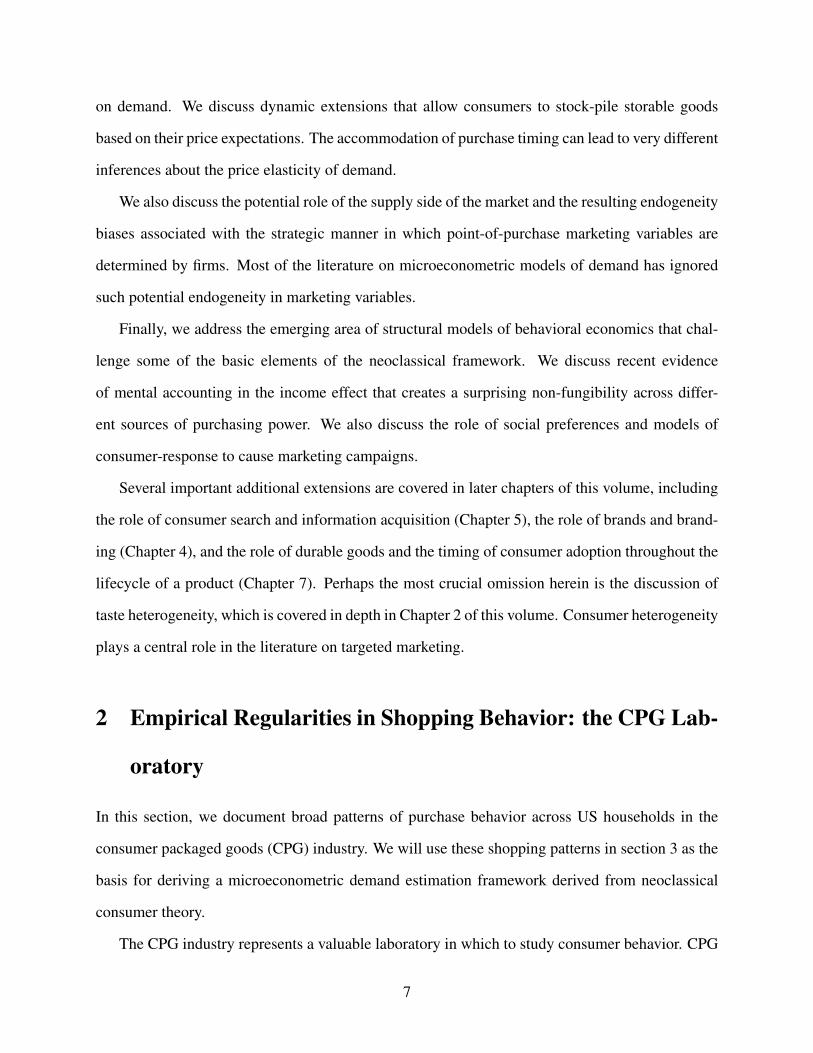
2 Empirical Regularities in Shopping Behavior: the CPG Lab-

oratory

In this section, we document broad patterns of purchase behavior across US households in the

consumer packaged goods (CPG) industry. We will use these shopping patterns in section 3 as the

basis for deriving a microeconometric demand estimation framework derived from neoclassical

consumer theory.

The CPG industry represents a valuable laboratory in which to study consumer behavior. CPG

7

brands are widely available across store formats including grocery stores, supermarkets, discount

and club stores, drug stores and convenience stores. They are also purchased at a relatively high

frequency. The average US household consumer conducted 1.7 grocery trips per week in 20174

Most importantly, CPG spending represents an sizable portion of household budgets. In 2014, the

global CPG sector was valued at $8 trillion and was predicted to grow to $14 trillion by 20255.

In 2016, US households spent $407 billion on CPGs6. A long literature in brand choice has used

household panel data in CPG categories not only due to the economic relevance, but also due to

the high quality of the data. CPG categories exhibit high-frequency price promotions that can be

exploited for demand estimation purposes.

We use the Nielsen Homescan panel housed by the Kilts Center for Marketing at the Univer-

sity of Chicago Booth School of Business to document CPG purchase patterns. The Homescan

panelists are nationally representative7. The database tracks purchases in 1,011 CPG product cat-

egories (denoted by Nielsen’s product modules codes) for over 132,000 households between 2004

and 2012, representing over 88 million shopping trips. Nielsen classifies product categories us-

ing module codes. Examples of product modules include Carbonated Soft Drinks, Ready-to-Eat

Cereals, Laundry Detergents and Tooth Paste.

We retain the 2012 transaction data to document several empirical regularities in shopping

behavior. In 2012, we observe 52,093 households making over 6.57 million shopping trips during

which they purchase over 46 million products.

The typical CPG category offers a wide amount of variety to consumers. Focusing only on

the products actually purchased by Homescan panelists in 2012, the average category offers 402.8

unique products as indexed by a universal product code (UPC) and 64.4 unique brands. For in-

4Source: “Consumers’ weekly grocery shopping trips in the United States from 2006 to 2017 ,” Statista, 2017, ac-cessed at https://www.statista.com/statistics/251728/weekly-number-of-us-grocery-shopping-trips-per-household/ on11/13/2017.

5Source: “Three myths about growth in consumer packaged goods,” by Rogerio Hirose, Renata Maia, AnneMartinez, and Alexander Thiel, McKinsey, June 2015, accessed at https://www.mckinsey.com/industries/consumer-packaged-goods/our-insights/three-myths-about-growth-in-consumer-packaged-goods on 11/13/2017.

6source: “Consumer packaged goods (CPG) expenditure of U.S. consumers from 2014 to 2020,” Statista,2017, accessed at https://www.statista.com/statistics/318087/consumer-packaged-goods-spending-of-us-consumers/on 11/13/2017

7See Einav, Leibtag, and Nevo (e.g., 2010) for a validation study of the Homescan data.

8

stance, a brand might be any UPC coded product with the brand name Coca Cola, whereas a UPC

might be a 6-pack of 12-oz cans of Coca Cola. While the subset of available brands and sizes

varies across stores and regions, these numbers reveal the extent of variety available to consumers.

In addition, CPG products are sold in pre-packaged, indivisible pack sizes. The average category

offers 31.9 different pack size choices. The average brand within a category is sold in 5.4 different

pack sizes. Therefore, consumers face an interesting indivisibility constraint, especially if they are

determined to buy a specific brand variant. Moreover, CPG firms’ widespread pre-commitment to

specific sizes is suggestive of extensive use of non-linear pricing.

For the average category, we observe 39,787 trips involving at least one purchase. Households

purchase a single brand and a single pack during 94.3% and 67.3% of the category-trip combina-

tions, respectively. On average, households purchase 1.07 brands per category-trip. In sum, the

discrete brand choice assumption, and to a lesser extent the discrete quantity choice assumption,

seems broadly appropriate across trips at the category level.

However, we do observe categories in which the contemporaneous purchase of assortments

is more commonplace and many of these categories are economically large. In the Ready-to-Eat

Cereals category, which ranks third overall in total household expenditures among all CPG cate-

gories, consumers purchase a single brand during only 72.6% of trips. Similarly, for Carbonated

Soft Drinks and Refrigerated Yogurt, which rank fourth and tenth overall respectively, consumers

purchase a single brand during only 81.5% and 86.6% of trips respectively. Therefore, case studies

of some of the largest CPG categories may need to consider demand models that allow for the

purchase of variety, even though only a small number of the variants is chosen on any given trip.

Similarly, we observe many categories where consumers occasionally purchase multiple packs of

a product, even when only a single brand is chosen. In these cases, a demand model that accounts

for the intensive margin of quantity purchased may be necessary.We also observe brand switching

across time within a category, especially in some of the larger categories. For instance, during

the course of the year, households purchased 7.5 brands of Ready-to-Eat Cereals (ranked 3rd),

5.9 brands of Cookies (ranked 11th), 4.7 brands of Bakery Bread (ranked 7th), and 4.6 brands of

9

Carbonated Soft Drinks (ranked 4th). In many of the categories with more than an average of 3

brands purchased per household-year, we typically observe only one brand being chosen during an

individual trip.

In summary, a snapshot of a single year of CPG shopping behavior by a representative sample

of consumers indicates some striking patterns. In spite of the availability of a large amount of

variety, on any given trip, consumers purchase only a very small number of variants. From a mod-

eling perspective, we observe a high incidence of corner solutions. In some of the largest product

categories, consumers routinely purchase assortments, leading to complex patterns of corner solu-

tions. In most categories, the corner solutions degenerate to a pure discrete choice scenario where

a single unit of a single product is purchased. In these cases, the standard discrete choice models

may be sufficient. However, the single unit is typically one of several pre-determined pack sizes

available suggesting an important role for indivisibility on the demand side, and non-linear pricing

on the supply side.

3 The Neoclassical Derivation of an Empirical Model of Indi-

vidual Consumer Demand

The empirical regularities in section 2 show that household-level demand for consumer goods ex-

hibit a high incidence of corner solutions: purchase occasions with zero expenditure on most items

in the choice set. The methods developed in the traditional literature on demand estimation (e.g.,

Deaton and Muellbauer, 1980b) do not accommodate zero consumption. In this section, we review

the formulation of the neoclassical consumer demand problem and the corresponding challenges

with the accommodation of corner solutions into an empirical framework. Our theoretical starting

point is the usual static model of utility maximization whereby the consumer spends a fixed budget

on a set of competing goods. Utility theory plays a particularly crucial role in accommodating the

empirical prominence of corner solutions in individual-level data.

10

3.1 The Neoclassical Model of Demand with Binding, Non-Negativity Con-

straints

We start with the premise that the analyst has access to marketing data comprising individual-level

transactions. The analyst’s data include the exact vector of quantities purchased by a customer on

a given shopping trip, x = (x1, ..., xJ+1)′. An individual transaction database typically has a panel

format with time-series observations (trips) for a cross section of customers. We assume that the

point-of-purchase causal environment consists of prices, but the database could also include other

marketing promotional variables. Our objective consists of deriving a likelihood for this observed

vector of purchases from microeconomic primitives. Suppose WLOG that the consumer does not

consume the first l goods: x j = 0 ( j = 1, ..., l), and x j > 0 ( j = l +1, ...,J+1) .

We use the neoclassical approach to deriving consumer demand from the assumption that each

consumer maximizes a utility function U (x;θ ,ε) defined over the quantity of goods consumed,

x=(x1, ...,xJ+1)′. Since most marketing studies focus on demand behavior within a specific “prod-

uct category,” we adopt the terminology of Becker (1965) and distinguish between the “commod-

ity” (e.g., the consumption benefit of the category, such as laundry detergent), and the j = 1, ...,J

“market goods” to which we will refer as “products” (e.g., the various brands sold within the

product category, such as Tide and Wisk laundry detergents). The quantities in x are non-negative

(x j ≥ 0 ∀ j) and satisfy the consumer’s budget constraint x′p 6 y, where p = (p1, ..., pJ+1)′ is a vec-

tor of strictly positive prices and y is the consumer’s budget. The vector θ consists of unknown (to

the researcher) parameters describing the consumer’s underlying preferences and the vector ε cap-

tures unobserved (to the researcher), mean-zero, consumer-specific utility disturbances8. Typically

ε is assumed to be known to the consumer prior to decision-making.

Formally, the utility maximization problem can be written as follows

V (p,y;θ ,ε)≡ max{x1,...,xJ}

{U (x;θ ,ε) : x′p 6 y, x≥ 0

}(1)

8It is straightforward to allow for additional persistent, unobserved taste heterogeneity by indexing the parametersthemselves by consumer (see Chapter 2 of this volume).

11

where we assume U (•;θ ,ε) is a continuously-differentiable, quasi-concave and increasing func-

tion9. We can define the corresponding Lagrangian function L = U (x;θ ,ε)+λy (y−p′x)+λ′xx

where λy and the vector λ x are Lagrange multipliers for the budget and non-negativity constraints

respectively.

A solution to (1) exists as long as the following necessary and sufficient Karush-Kuhn-Tucker

(KKT) conditions hold

∂U(x∗;θ ,ε)∂x j

−λy p j +λx, j = 0 , j = 1, ...,J+1

y−p′x∗ = 0, (y−p′x∗)λy = 0, λy > 0

x∗j ≥ 0, x∗jλx, j = 0, λx, j ≥ 0 j = 1, ...,J+1.

(2)

Since U (•;θ ,ε) is increasing, the consumer spends her entire budget (the “adding-up” condition)

and at least one good will always be consumed. We define the J + 1 good as an “essential” nu-

meraire with corresponding price pJ+1 = 1 and with preferences that are separable from those over

the commodity group10. We assume additional regularity conditions on U (•;θ ,ε) to ensure that

an interior quantity of J + 1 is always consumed: ∂U(x∗;θ ,ε)∂xJ+1

= λy and λx,J+1 = 0. We can now

re-write the KKT conditions as follows

∂U(x∗;θ ,ε)∂x j

− ∂U(x∗;θ ,ε)∂xJ+1

p j +λx, j = 0 , j = 1, ...,J

y−p′x∗ = 0

x∗j ≥ 0, x∗jλx, j = 0, λx, j ≥ 0 j = 1, ...,J.

(3)

For our observed consumer, recall that x j = 0 ( j = 1, ..., l) and x j > 0 ( j = l +1, ...,J+1) . We

9These sufficient conditions ensure the existence of a demand function with a unique consumption level thatmaximizes utility at a given set of prices (e.g., Mas-Collel, Whinston, and Green, 1995, chapter 3)

10The essential numeraire is typically interpreted as expenditures outside of the commodity group(s) of interest.

12

can now re-write the KKT conditions to capture these non-consumption decisions

∂U(x∗;θ ,ε)∂x j

− ∂U(x∗;θ ,ε)∂xJ+1

p j ≤ 0 , j = 1, ..., l

∂U(x∗;θ ,ε)∂x j

− ∂U(x∗;θ ,ε)∂xJ+1

p j = 0 , j = l +1, ...,J

(4)

It is instructive to consider how the KKT conditions (4) influence demand estimation. The

l + 1 to J equality conditions in (4) implicitly characterize the conditional demand equations for

the purchased goods. The l inequality conditions in (4) give rise to the following demand regime-

switching conditions, or “selection” conditions

∂U(x∗;θ ,ε)∂x j

∂U(x∗;θ ,ε)∂xJ+1

≤ p j, j = 1, ..., l (5)

which determine whether a given product’s prices are above the consumer’s reservation value,∂U(x∗;θ ,ε)

∂x j∂U(x∗;θ ,ε)

∂xJ+1

(see Lee and Pitt, 1986; Ransom, 1987, for a discussion of the switcing regression inter-

pretation). We can now see how dropping the observations with zero consumption will likely result

in selection bias due to the correlation between the switching probabilities and the utility shocks,

ε .

To complete the model, we need to allow for some separability of the utility disturbances. For

instance, we can assume an additive, stochastic log-marginal utility: ln(

∂U(x∗;θ ,ε)∂x j

)= ln

(U j (x∗;θ)

)+

ε j for each j, where U j (x∗;θ) is deterministic. We also assume that ε are random variables with

known distribution and density, F (ε) and f (ε) respectively. We can now write the KKT conditions

more compactly:

ε j ≡ ε j− εJ+1 ≤ h j (x∗;θ) , j = 1, ..., l

ε j ≡ ε j− εJ+1 = h j (x∗;θ) , j = l +1, ...,J

(6)

where h j (x∗;θ) = ln(UJ+1 (x∗;θ))− ln(U j (x∗;θ)

)+ ln

(p j)

.

We can now derive the likelihood function associated with the observed consumption vector, x.

13

In the case where all the goods are consumed, then the density of x is

fx (x;θ) = fε (ε) |J (x) | (7)

where J (x) is the Jacobian of the transformation from ε to x. If only the J +1 numeraire good is

consumed, the density of x = (0, ...,0) is

fx (x;θ) =∫ hJ(x;θ)

−∞

· · ·∫ h1(x;θ)

−∞

fε (ε)dε1 · · ·dεJ. (8)

For the more general case in which the first l goods are not consumed, the density of x=(0, ...,0, xl+1, ..., xJ)

is

fx (x;θ) =∫ hl(x;θ)

−∞

· · ·∫ h1(x;θ)

−∞

fε (ε1, ..., εl,hl+1 (x;θ) , ...,hJ (x;θ)) |J (x) |dε1 · · ·dεl (9)

where J (x) is the Jacobian of the transformation from ε to (xl+1, ...,xJ) when (x1, ...,xl) = 0.

Suppose the researcher has a data sample with i = 1, ...,N independent consumer purchase

observations. The sample likelihood is

L (θ |x) =N

∏i=1

fx (xi) . (10)

A maximum likelihood estimate of θ based on (10) is consistent and asymptotically efficient.

3.1.1 Estimation Challenges with the Neoclassical Model

van Soest, Kapteyn, and Kooreman (1993) have shown that the choice of functional form to ap-

proximate utility, U (x) , can influence consistency of the maximum likelihood estimator based on

(10). In particular, the KKT conditions in (2) generate a unique vector x∗ (p,y;θ ,ε) at given (p,y)

for all possible θ and ε as long as U (x) is monotonic and strictly quasi-concave. When these

conditions fail to hold, the system of KKT conditions (2) may not generate a unique solution,

x∗ (p,y;θ ,ε) . This non-uniqueness leads to the well-known coherency problem with maximum

14

likelihood estimation (Heckman, 1978)11, which can lead to inconsistent estimates. Note that the

term coherency is used slightly differently in the more recent literature on empirical games with

multiple equilibria. Tamer (2003) uses the term coherency in reference to the sufficient condi-

tions for the existence of a solution x∗ (p,y;θ ,ε) to the model (in this case x∗ satisfies the KKT

conditions). He uses the term model completeness in reference to the case where these sufficient

conditions for the statistical model to have a well-defined likelihood. For our neoclassical model of

demand, the econometric model would be termed “incomplete” if demand was a correspondence

and, hence, there were multiple values of x∗ that satisfy the KKT conditions at a given (p,y;θ ,ε) .

van Soest, Kapteyn, and Kooreman (1993) propose a set of parameter restrictions that are suf-

ficient for coherency. For many specifications, these conditions will only ensure that the regularity

of U (x) holds over the set of prices and quantities observed in the data. While these conditions

may suffice for estimation, failure of the global regularity condition could be problematic for pol-

icy simulations that use the demand estimates to predict outcomes outside the range of observed

values in the sample. For many specifications, the parameter restrictions may not have an analytic

form, and may require numerical tools to impose them. As we will see in the examples below,

the literature has often relied on special functional forms, with properties like additivity and ho-

motheticity, to ensure global regularity and to satisfy the coherency conditions. However, these

specifications come at the cost of less flexible substitution patterns.

In addition to coherency concerns, maximum likelihood estimation based on equation (9) also

involves several computational challenges. If the system of KKT conditions does not generate a

closed-form expression for the conditional demand equations, it may be difficult to impose co-

herency conditions. In addition, the likelihood comprises a density component for the goods with

non-zero consumption and a mass component for the corners at which some of the goods have an

optimal demand of zero. The mass component in (9) requires evaluating an l-dimensional integral

over a region defined implicitly by the solution to the KKT conditions (4). When consumers pur-

11Coherency pertains to the case where there is a unique vector x∗ generated by the KKT conditions correspondingto each possible value of ε , and there is a unique value of ε that generates each possible vector x∗generated by theKKT conditions.

15

chase l of the alternatives, there are

J

l

potential shopping baskets, and each of the observed

combinations would need to be solved. The likelihood also involves two change-of-variables from

ε to ε and from ε to x respectively, requiring the computation of a Jacobian matrix.

Estimation methods are beyond the scope of this discussion. However, a number of papers

have proposed methods to accommodate several of the computational challenges above including

simulated maximum likelihood (Kao, fei Lee, and Pitt, 2001), hierarchical Bayesian algorithms

that use MCMC methods based on Gibbs sampling (Millimet and Tchernis, 2008), hybrid methods

that combine Gibbs sampling with Metropolis-Hastings (Kim, Allenby, and Rossi, 2002), and

GMM estimation (Thomassen, Seiler, Smith, and Schiraldi, 2017).

In the remainder of this section, we discuss several examples of functional forms for U (x) that

have been implemented in practice.

3.1.2 Example: Quadratic Utility

Due to its tractability, the quadratic utility,

U (x;θ ,ε) =J+1

∑j=1

(β j0 + ε j

)x j +

12

J+1

∑j=1

J+1

∑k=1

β jkx jxk (11)

has been a popular functional form for empirical work (e.g., Wales and Woodland, 1983; Ransom,

1987; Lambrecht, Seim, and Skiera, 2007; Mehta, 2015; Yao, Mela, Chiang, and Chen, 2012;

Thomassen, Seiler, Smith, and Schiraldi, 2017)12. The random utility shocks in (11) are “ran-

dom coefficients” capturing heterogeneity across consumers in the linear utility components over

the various products. Assume WLOG that the consumer foregoes consumption on goods x j = 0

( j = 1, ..., l), and chooses a positive quantity for goods x j > 0 ( j = l +1, ...,J+1) . The corre-

sponding KKT conditions are

12Thomassen, Seiler, Smith, and Schiraldi (2017) extend the quadratic utility model to allow for discrete storechoice as well as the discrete/continuous expenditure allocation decisions across grocery product categories within avisited store.

16

ε j +β j0 +∑J+1k=1 β jkx∗j −

(βJ+1,0 +∑

J+1k=1 βJ+1,kx∗J+1

)p j ≤ 0 , j = 1, ..., l

ε j +β j0 +∑J+1k=1 β jkx∗j −

(βJ+1,0 +∑

J+1k=1 βJ+1,kx∗J+1

)p j = 0 , j = l +1, ...,J

(12)

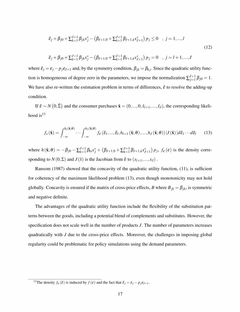
where ε j = ε j− p jεJ+1 and, by the symmetry condition, β jk = βk j. Since the quadratic utility func-

tion is homogeneous of degree zero in the parameters, we impose the normalization ∑J+1j=1 β j0 = 1.

We have also re-written the estimation problem in terms of differences, ε to resolve the adding-up

condition.

If ε ∼ N(0, Σ)

and the consumer purchases x = (0, ...,0, xl+1, ..., xJ), the corresponding likeli-

hood is13

fx (x) =∫ hl(x;θ)

−∞

· · ·∫ h1(x;θ)

−∞

fε (ε1, ..., εl,hl+1 (x;θ) , ...,hJ (x;θ)) |J (x) |dε1 · · ·dεl (13)

where h(x;θ) = −β j0−∑J+1k=1 βkix∗j +

(βJ+1,0 +∑

J+1k=1 βJ+1,kx∗J+1

)p j, fε (ε) is the density corre-

sponding to N (0,Σ) and J (x) is the Jacobian from ε to (xl+1, ...,xJ) .

Ransom (1987) showed that the concavity of the quadratic utility function, (11), is sufficient

for coherency of the maximum likelihood problem (13), even though monotonicity may not hold

globally. Concavity is ensured if the matrix of cross-price effects, B where B jk = β jk, is symmetric

and negative definite.

The advantages of the quadratic utility function include the flexibility of the substitution pat-

terns between the goods, including a potential blend of complements and substitutes. However, the

specification does not scale well in the number of products J. The number of parameters increases

quadratically with J due to the cross-price effects. Moreover, the challenges in imposing global

regularity could be problematic for policy simulations using the demand parameters.

13The density fε (ε) is induced by f (ε) and the fact that ε j = ε j− p jεJ+1.

17

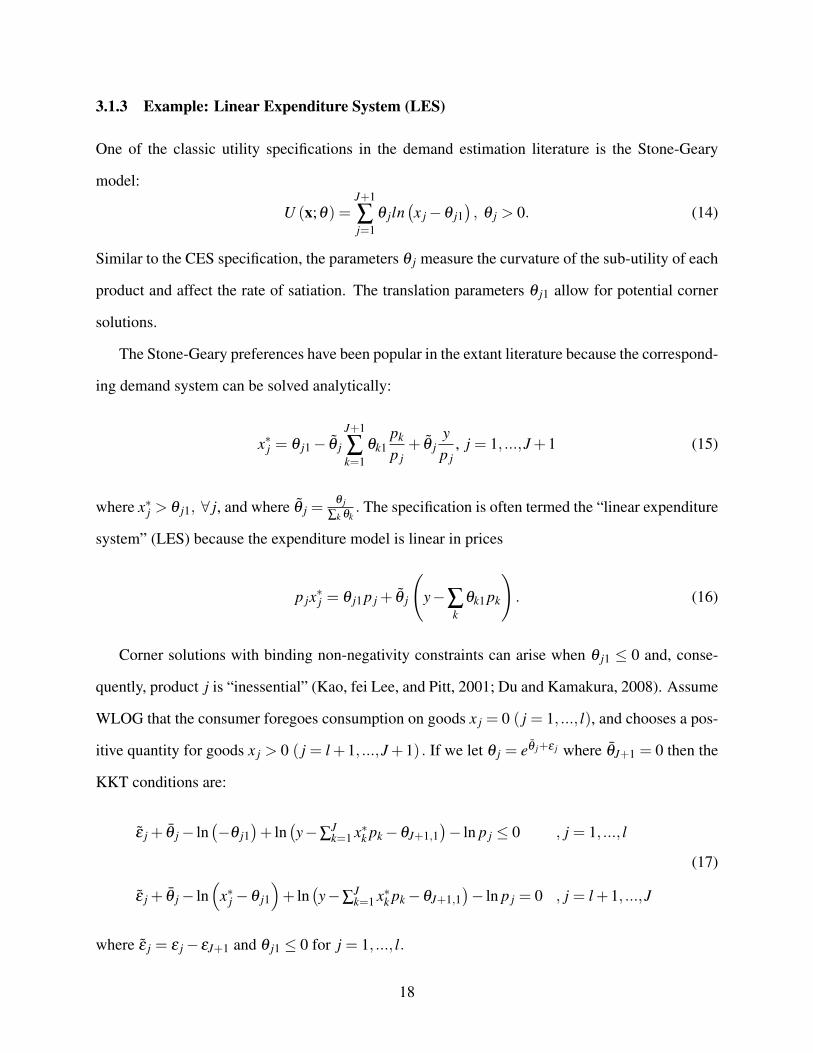
3.1.3 Example: Linear Expenditure System (LES)

One of the classic utility specifications in the demand estimation literature is the Stone-Geary

model:

U (x;θ) =J+1

∑j=1

θ jln(x j−θ j1

), θ j > 0. (14)

Similar to the CES specification, the parameters θ j measure the curvature of the sub-utility of each

product and affect the rate of satiation. The translation parameters θ j1 allow for potential corner

solutions.

The Stone-Geary preferences have been popular in the extant literature because the correspond-

ing demand system can be solved analytically:

x∗j = θ j1− θ j

J+1

∑k=1

θk1pk

p j+ θ j

yp j

, j = 1, ...,J+1 (15)

where x∗j > θ j1, ∀ j, and where θ j =θ j

∑k θk. The specification is often termed the “linear expenditure

system” (LES) because the expenditure model is linear in prices

p jx∗j = θ j1 p j + θ j

(y−∑

kθk1 pk

). (16)

Corner solutions with binding non-negativity constraints can arise when θ j1 ≤ 0 and, conse-

quently, product j is “inessential” (Kao, fei Lee, and Pitt, 2001; Du and Kamakura, 2008). Assume

WLOG that the consumer foregoes consumption on goods x j = 0 ( j = 1, ..., l), and chooses a pos-

itive quantity for goods x j > 0 ( j = l +1, ...,J+1) . If we let θ j = eθ j+ε j where θJ+1 = 0 then the

KKT conditions are:

ε j + θ j− ln(−θ j1

)+ ln

(y−∑

Jk=1 x∗k pk−θJ+1,1

)− ln p j ≤ 0 , j = 1, ..., l

ε j + θ j− ln(

x∗j −θ j1

)+ ln

(y−∑

Jk=1 x∗k pk−θJ+1,1

)− ln p j = 0 , j = l +1, ...,J

(17)

where ε j = ε j− εJ+1 and θ j1 ≤ 0 for j = 1, ..., l.

18

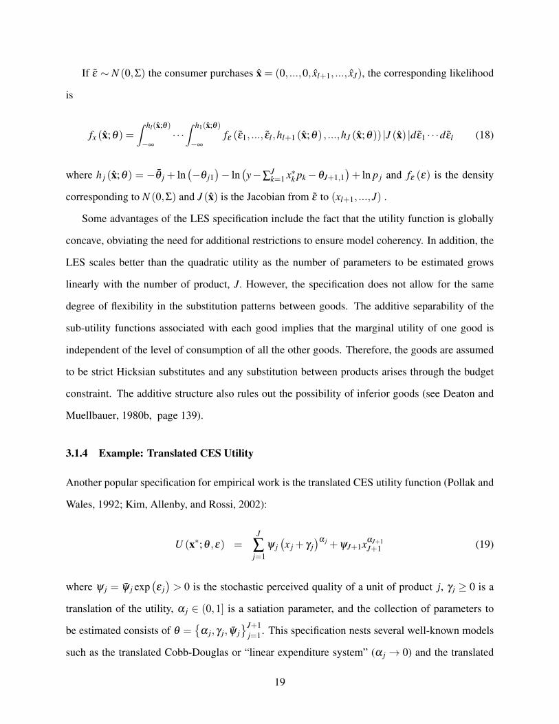
If ε ∼ N (0,Σ) the consumer purchases x = (0, ...,0, xl+1, ..., xJ), the corresponding likelihood

is

fx (x;θ) =∫ hl(x;θ)

−∞

· · ·∫ h1(x;θ)

−∞

fε (ε1, ..., εl,hl+1 (x;θ) , ...,hJ (x;θ)) |J (x) |dε1 · · ·dεl (18)

where h j (x;θ) = −θ j + ln(−θ j1

)− ln

(y−∑

Jk=1 x∗k pk−θJ+1,1

)+ ln p j and fε (ε) is the density

corresponding to N (0,Σ) and J (x) is the Jacobian from ε to (xl+1, ...,J) .

Some advantages of the LES specification include the fact that the utility function is globally

concave, obviating the need for additional restrictions to ensure model coherency. In addition, the

LES scales better than the quadratic utility as the number of parameters to be estimated grows

linearly with the number of product, J. However, the specification does not allow for the same

degree of flexibility in the substitution patterns between goods. The additive separability of the

sub-utility functions associated with each good implies that the marginal utility of one good is

independent of the level of consumption of all the other goods. Therefore, the goods are assumed

to be strict Hicksian substitutes and any substitution between products arises through the budget

constraint. The additive structure also rules out the possibility of inferior goods (see Deaton and

Muellbauer, 1980b, page 139).

3.1.4 Example: Translated CES Utility

Another popular specification for empirical work is the translated CES utility function (Pollak and

Wales, 1992; Kim, Allenby, and Rossi, 2002):

U (x∗;θ ,ε) =J

∑j=1

ψ j(x j + γ j

)α j +ψJ+1xαJ+1J+1 (19)

where ψ j = ψ j exp(ε j)> 0 is the stochastic perceived quality of a unit of product j, γ j ≥ 0 is a

translation of the utility, α j ∈ (0,1] is a satiation parameter, and the collection of parameters to

be estimated consists of θ ={

α j,γ j, ψ j}J+1

j=1. This specification nests several well-known models

such as the translated Cobb-Douglas or “linear expenditure system” (α j → 0) and the translated

19

Leontieff (α j →−∞). For any product j, setting γ j = 0 would ensure a strictly interior quantity,

x∗j > 0.

The logarithmic form of the KKT conditions associated with the translated CES utility model

areε j ≤ h j

(x∗j ;θ

), j = 1, ..., l

ε j = h j

(x∗j ;θ

), j = l +1, ...,J

(20)

where h j

(x∗j ;θ

)= ln

(ψJ+1αJ+1

(x∗j)αJ+1−1

)− ln

(ψ jα j

(x∗j + γ j

)α j−1)+ ln

(p j)

and ε j =

ε j− εJ+1.

If ε ∼ N (0,Σ) and the consumer purchases x = (0, ...,0, xl+1, ..., xJ), the corresponding likeli-

hood is

fx (x;θ) =∫ hl(x;θ)

−∞

· · ·∫ h1(x;θ)

−∞

fε (ε1, ..., εl,hl+1 (x;θ) , ...,hJ (x;θ)) |J (x) |dε1 · · ·dεl. (21)

where fε (ε) is the density corresponding to N (0,Σ) and J (x) is the Jacobian from ε to (xl+1, ...,J).

If instead we assume ε ∼ i.i.d. EV (0,σ), Bhat (2005) and Bhat (2008) derive the simpler, closed-

form expression for the likelihood with analytic solutions to the integrals and the Jacobian J (x) in

(21)

fx (x;θ) =1

σ J−l

[J+1

∏i=l+1

fi

][J+1

∑i=l+1

pi

fi

]∏

J+1i=l+1 e

hi(x∗i ;θ)σ(

∑J+1j=1 e

h j(x∗k ;θ)σ

)J−l+1

(J− l)!

where, changing the notation from above slightly, we define h j

(x∗j ;θ

)= ψ j+

(α j−1

)ln(

x∗j + γ j

)−

ln(

p j)

and fi =(

1−αix∗i +γi

).

A formulation of the utility function specifies an additive model of utility over stochastic con-

20

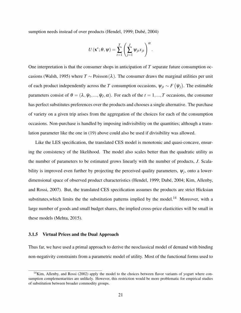
sumption needs instead of over products (Hendel, 1999; Dubé, 2004)

U (x∗;θ ,ψ) =T

∑t=1

(J

∑j=1

ψ jtx jt

)α

.

One interpretation is that the consumer shops in anticipation of T separate future consumption oc-

casions (Walsh, 1995) where T ∼ Poisson(λ ). The consumer draws the marginal utilities per unit

of each product independently across the T consumption occasions, ψ jt ∼ F(ψ j). The estimable

parameters consist of θ = (λ , ψ1, ..., ψJ,α). For each of the t = 1, ...,T occasions, the consumer

has perfect substitutes preferences over the products and chooses a single alternative. The purchase

of variety on a given trip arises from the aggregation of the choices for each of the consumption

occasions. Non-purchase is handled by imposing indivisibility on the quantities; although a trans-

lation parameter like the one in (19) above could also be used if divisibility was allowed.

Like the LES specification, the translated CES model is monotonic and quasi-concave, ensur-

ing the consistency of the likelihood. The model also scales better than the quadratic utility as

the number of parameters to be estimated grows linearly with the number of products, J. Scala-

bility is improved even further by projecting the perceived quality parameters, ψ j, onto a lower-

dimensional space of observed product characteristics (Hendel, 1999; Dubé, 2004; Kim, Allenby,

and Rossi, 2007). But, the translated CES specification assumes the products are strict Hicksian

substitutes,which limits the the substitution patterns implied by the model.14 Moreover, with a

large number of goods and small budget shares, the implied cross-price elasticities will be small in

these models (Mehta, 2015).

3.1.5 Virtual Prices and the Dual Approach

Thus far, we have used a primal approach to derive the neoclassical model of demand with binding

non-negativity constraints from a parametric model of utility. Most of the functional forms used to

14Kim, Allenby, and Rossi (2002) apply the model to the choices between flavor variants of yogurt where con-sumption complementarities are unlikely. However, this restriction would be more problematic for empirical studiesof substitution between broader commodity groups.

21

approximate utility in practice impose restrictions motivated by technical convenience. As we saw

above, these restrictions can limit the flexibility of the demand model on factors such as substitution

patterns between products and income effects. For instance, the additivity assumption resolves the

global regularity concerns, but restricts the products to be strict substitutes. Accommodating more

flexible substitution patterns becomes computationally difficult even for a simple specification like

quadratic utility due to the coherency conditions.

The dual approach has been used to derive demand systems from less restrictive assumptions

Deaton and Muellbauer (1980b). Lee and Pitt (1986) developed an approach to use duality to

derive demand while accounting for with binding non-negativity constraints using virtual prices.

The advantage of the dual approach is that a flexible functional form can be used to approximate

indirect utility and cost functions can be used to determine the relevant restrictions to ensure that

the derived demand system is consistent with microeconomic principles. The trade-off from using

this dual approach is that the researcher loses the direct connection between the demand parameters

and their deep structural interpretation as specific aspects of “preferences.” The specifications may

be less suitable for marketing applications to problems such as product design, consumer quality

choice and the valuation of product features, these specifications.

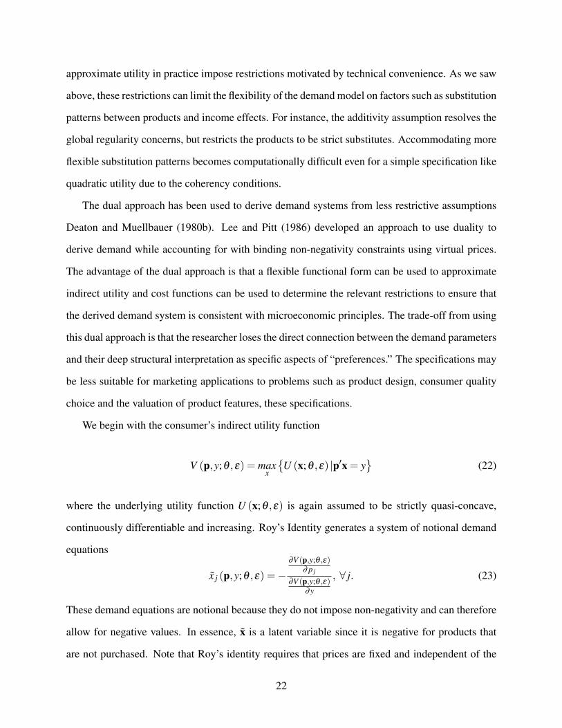
We begin with the consumer’s indirect utility function

V (p,y;θ ,ε) = maxx

{U (x;θ ,ε) |p′x = y

}(22)

where the underlying utility function U (x;θ ,ε) is again assumed to be strictly quasi-concave,

continuously differentiable and increasing. Roy’s Identity generates a system of notional demand

equations

x j (p,y;θ ,ε) =−∂V (p,y;θ ,ε)

∂ p j

∂V (p,y;θ ,ε)∂y

, ∀ j. (23)

These demand equations are notional because they do not impose non-negativity and can therefore

allow for negative values. In essence, x is a latent variable since it is negative for products that

are not purchased. Note that Roy’s identity requires that prices are fixed and independent of the

22

quantties purchased by the consumer, an assumption that fails in settings where firms use non-

linear pricing such as promotional quantity discounts15.

Lee and Pitt (1986) use virtual prices to handle products with zero quantity demanded (Neary

and Roberts, 1980). Suppose the consumer’s optimal consumption vector is x∗=(0, ...,0,x∗l+1, ..,x

∗J+1)

where, as before, she does not purchase the first l goods. We can define virtual prices based on

Roy’s Identity in equation (23) that exactly set the notional demands to zero for the non-purchased

goods

0 =∂V (π (p,y;θ ,ε) , p,y;θ ,ε)

∂ p j, j = 1, .., l.

where π (p,y;θ ,ε) = (π1 (p,y;θ ,ε) , ...,πl (p,y;θ ,ε)) is the l-vector of virtual prices and p =

(pl+1, ..., pJ). These virtual prices act like reservation prices for the non-purchased goods. We

can derive the positive demands for goods j = l+1, ...,J+1 by substituting the virtual prices into

Roy’s identity:

x∗j (p,y;θ ,ε) =−∂V (π(p,y;θ ,ε),p,y;θ ,ε)

∂ p j

∂V (π(p,y;θ ,ε),p,y;θ ,ε)∂y

, j = l +1, ...,J+1. (24)

The regime switching conditions in which products j = 1, ..., l are not purchased consist of com-

paring virtual prices and observed prices:

π j (p,y;θ ,ε)≤ p j, j = 1, ..., l. (25)

Lee and Pitt (1986) demonstrate the parallel between the switching conditions based on virtual

prices in (25) and the binding non-negativity constraints in the KKT conditions, (4).

The demand parameters θ can then be estimated by combining the conditional demand system,

(24), and the regime-switching conditions, (4). If the consumer purchases x=(0, ...,0, xl+1, ..., xJ+1),

15Howell, Lee, and Allenby (2016) show how a primal approach with a parametric utility specification can be usedin the presence of non-linear pricing.

23

the corresponding likelihood is

fx (x;θ)=∫

∞

π−1l (p,y,pl ;θ)

· · ·∫

∞

π−11 (p,y,p1;θ)

fε

(ε1, ...,εl,x∗−1

l+1 (x, p,y;θ) , ...,x∗−1J (x, p,y;θ)

)|J (x) |dε1 · · ·dεl.

(26)

where fε (ε) is the density corresponding to N (0,Σ) and J (x) is the Jacobian from ε to (xl+1, ...,xJ).

The inverse functions in (26) reflect the fact that π−1j(p,y, p j;θ

)≤ ε j for j = 1, ..., l and x∗−1

j (x, p,y;θ)=

ε j for j = l +1, ...,J.

As with the primal problem, the choice of functional form for the indirect utility, V (p,y;θ ,ε),

can influence the coherency of the maximum likelihood estimator for θ in (26). van Soest,

Kapteyn, and Kooreman (1993) show that the uniqueness of the demand function defined by Roy’s

Identity in (23) will hold if the indirect utility function V (p,y;θ ,ε) satisfies the following three

regularity conditions:

1. V (p,y;θ ,ε) is homogeneous of degree zero

2. V (p,y;θ ,ε) is twice continuously differentiable in p and y

3. V (p,y;θ ,ε) is regular, meaning that the Slutsky matrix is negative semi-definite (“negativ-

ity”)

For many popular and convenient flexible functional forms, the Slutsky matrix may fail to satisfy

negativity leading to the coherency problem. In many of these cases, such as AIDS, the virtual

prices may need to be derived numerically, making it difficult to derive analytic restrictions that

would ensure these regularity conditions hold. For these reasons, the homothetic translog specifi-

cation discussed below has been extremely popular in practice.

3.1.6 Example: Indirect Translog Utility

One of the most popular implementations of the dual approach described above in section (3.1.5)

uses the translog approximation of the indirect utility function (e.g., Lee and Pitt, 1986; Millimet

24

and Tchernis, 2008; Mehta, 2015)

V (p,y;θ ,ε) =J+1

∑j=1

θ j ln(

p j

y

)+

12

J+1

∑j=1

J+1

∑k=1

θ jk ln(

p j

y

)ln(

pk

y

). (27)

The econometric error is typically introduced by assuming θ j = θ j + ε j where ε j ∼ F (ε) .

Roy’s Identity gives us the notional expenditure share for product jCHE

s j =−θ j−∑

J+1k=1 θ jk ln pk

y

1−∑k ∑l θkl ln(

ply

) . (28)

Soest and Kooreman (1990) derived slightly weaker sufficient conditions for coherency of the

translog approach than van Soest, Kapteyn, and Kooreman (1993). Following Soest and Kooreman

(1990), we impose the following additional restrictions which are sufficient for the concavity of

the underlying utility function and, hence, the uniqueness of the demand system (28) for a given

realization of ε:θJ+1 = 1−∑ j θ j

∑k θ jk = 0, ∀ j

θ jk = θk j, ∀ j

(29)

We can re-write the expenditure share for product j

s j =−θ j−∑Jk=1 θ jk ln pk. (30)

We can see from (30) that an implication of the restrictions in (29) is that they also impose

homotheticity on preferences. For the translog specification, Mehta (2015) derived necessary and

sufficient conditions for global regularity that are even weaker than the conditions in Soest and

Kooreman (1990). These conditions allow for more flexible income effects (normal and inferior

goods) and for more flexible substitution patterns (substitutes and complements), mainly by relax-

25

ing homotheticity.16

3.2 The Discrete/Continuous Product Choice Restriction in the Neoclassical

Model

Perhaps due to their computational complexity, the application of the microeconometric models of

variety discussed in section (3) has been limited. However, the empirical regularities documented

in section (2) suggest that simpler models of discrete choice, with only a single product being

chosen, could be used in many settings. Recall from section (2) that the average category has a

single product choice chosen during 97% of trips. We now examine how our demand framework

simplifies under discrete product choice. The discussion herein follows Hanemann (1984); Chiang

and Lee (1992); Chiang (1991); Chintagunta (1993).

3.2.1 The Primal Problem

The model in this section closely follows the simple re-packaging model with varieties from Deaton

and Muellbauer (1980b). In these models, the consumption utility for a given product is based on

its effective quantity consumed, which scales the quantity by the product’s quality. As before, we

assume the commodity group of interest comprises j = 1, ...,J substitute products. Products are

treated as perfect substitutes so that, at most, a single variant is chosen. We also assume there is an

additional essential numeraire good indexed as product J+1.

To capture discrete product choice within the commodity group, we assume the following

bivariate utility over the commodity group and the essential numeraire:

U (x∗;θ ,ψ) = U

(J

∑j=1

ψ jx j,ψJ+1xJ+1

). (31)

The parameter vector ψ = (ψ1, ...,ψJ+1), ψ j ≥ 0 measures the constant marginal utility of each

16In an empirical application to consumer purchases over several CPG product categories, Mehta (2015) finds theproposed model fits the data better than the homothetic translog specification. However, when J = 2, the globallyregular translog will exhibit the restrictive strict Hicksian substitutes property.

26

of the products. In the literature, we often refer to ψ j as the “perceived quality” of product j.

Specifying the perceived qualities as random variables, ψ ∼ F (ψ), introduces random utility as a

potential source of heterogeneity across consumers in their perceptions of product quality. We also

assume regularity conditions on U (x∗;θ ,ψ) to ensure that a positive quantity of xJ+1 is always

chosen.

To simplify the notation, let the total commodity vector be z1 =∑Jj=1 ψ jx j and let z2 =ψJ+1xJ+1

so that we can re-write utility as U (z1,z2). The KKT conditions are

∂U(ψ ′x,ψJ+1xJ+1)∂ z1

ψ j− ∂U(ψ ′x,ψJ+1xJ+1)∂ z2

ψJ+1 p j ≤ 0 , j = 1, ...,J (32)

where ∂U(ψ ′x,ψJ+1xJ+1)∂ z1

is the marginal utility of total quality-weighted consumption within the com-

modity group. Because of the perfect substitutes specification, if a product within the commodity

group is chosen, it will be product k if

pk

ψk= min

{p j

ψ j

}J

j=1

and, hence, k exhibits the lowest price-to-quality ratio. As with the general model in section

(3), demand estimation will need to handle the regime switching, or demand selection conditions.

If pk >

∂U(z∗1,z∗2;θ ,ψ)

∂ z1ψk

∂U(z∗1,z∗2;θ ,ψ)

∂ z2ψJ+1

, then the consumer spends her entire budget on the numeraire: x∗J+1 =

y. Otherwise, the consumer allocates her budget between x∗k and x∗J+1 to equate∂U(z∗1,z

∗2;θ ,ψ)

∂ z1ψk

pk=

∂U(z∗1,z∗2;θ ,ψ)

∂ z2ψJ+1.

We define h j (x∗;θ ,ψ) =p jψJ+1

∂U(z∗1,z∗2;θ ,ψ)

∂ z2∂U(z∗1,z

∗2;θ ,ψ)

∂ z1

. When none of the products are chosen, we can

write the likelihood of x = (0, ...,0) as

fx (x;θ) =∫

∞

−∞

∫ hJ(x;θ ,ψJ+1)

−∞

· · ·∫ h1(x;θ ,ψJ+1)

−∞

fψ (ψ)dψ1 · · ·dψJ+1. (33)

27

When product 1 (WLOG) is chosen, we can write the likelihood of x = (x1,0, ..., ,0) as

fx (x;θ) =∫

∞

−∞

∫ hJ(x;θ ,ψJ+1)

−∞

· · ·∫ h2(x;θ ,ψJ+1)

−∞

fψ (h1 (x;θ ,ψ) ,ψ2, ...,ψJ+1) |J (x) |dψ2 · · ·dψJ+1

(34)

where J (x) is the Jacobian from ψ1 to x1. The likelihood now comprises a density component for

the chosen alternative j = 1, and a mass function for the remaining goods.

3.2.2 Example: Translated CES Utility

Recall the translated CES utility function presented in section (3.1.4)(Bhat, 2005; Kim, Allenby,

and Rossi, 2002):

U (x∗;θ ,ε) =J

∑j=1

ψ j(x j + γ j

)α j +ψJ+1xαJ+1J+1 .

We can impose discrete product choice with the restrictions α j = 1, γ j = 0 for j = 1, ...,J, which

gives us perfect substitutes utility over the brands

U (x∗;θ ,ε) =J

∑j=1

ψ jx j +ψJ+1xαJ+1.

Let ψ j = exp(ψ jε j

), j = 1, ...,J and ψJ+1 = exp(εJ+1), where ε j ∼ i.i.d. EV (0,σ) (Deaton

and Muellbauer, 1980a; Bhat, 2008). When none of the products are chosen, we can write the

likelihood of x = (0, ...,0) as

fx (x) =1

1+∑Jj=1 exp

(ψ j−ln(p j)−ln(αy(α−1))

σ

)

which is the multinomial logit model. If WLOG alternative 1 is chosen in the commodity group,

the likelihood of x = (x1, ...,0) is

28

f (x;θ)

=∫

∞

−∞1

σP1exp(−h1(ψJ+1;x1,p,θ)

σ

)exp[− 1

P1exp[

(−h1(ψJ+1;x1,p,θ)

σ

)](α−1y−x1

)fε (εJ+1)dεJ+1

=(

α−1y−x1

)1σ

∫∞

−∞exp(−εJ+1

σ

)∑

Jj=1 exp

(V jσ

)∏ j exp

[−exp

(−εJ+1

σ

)exp(

V jσ

)]fε (εJ+1)dεJ+1

where

Vj ≡ ψ j− ln(

p j)

and

h j (ψJ+1; x1,p,θ) = ln(

ψJ+1α (y− x1)α−1)+ ln

(p j)− ψ j

and

Pk ≡ P(εk + ψk− ln(pk)≥ ε j + ψ j− ln

(p j), j = 1, ...,J

)=

exp(

ψk−ln(pk)σ

)∑

Jj=1 exp

(ψ j−ln(p j)

σ

) .

3.2.3 Example: the Dual Problem with Indirect Translog Utility

Muellbauer (1974) has shown that maximizing the simple re-packaging model utility function in

(31) generates a bivariate indirect utility function of the form V(

pkψky ,

1ψJ+1y

)when product k is

the preferred product in the commodity group of interest. Following the template in Hanemann

(1984), several empirical studies of discrete/continuous brand choice have been derived based

on the indirect utility function and the dual virtual prices. For instance, Chiang (1991) and Arora,

Allenby, and Ginter (1998) use a second-order flexible translog approximation of the indirect utility

29

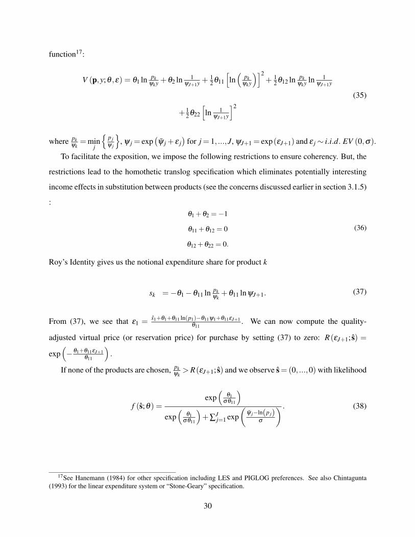
function17:

V (p,y;θ ,ε) = θ1 ln pkψky +θ2 ln 1

ψJ+1y +12θ11

[ln(

pkψky

)]2+ 1

2θ12 ln pkψky ln 1

ψJ+1y

+12θ22

[ln 1

ψJ+1y

]2

(35)

where pkψk

=minj

{p jψ j

}, ψ j = exp

(ψ j + ε j

)for j = 1, ...,J, ψJ+1 = exp(εJ+1) and ε j∼ i.i.d. EV (0,σ).

To facilitate the exposition, we impose the following restrictions to ensure coherency. But, the

restrictions lead to the homothetic translog specification which eliminates potentially interesting

income effects in substitution between products (see the concerns discussed earlier in section 3.1.5)

:θ1 +θ2 =−1

θ11 +θ12 = 0

θ12 +θ22 = 0.

(36)

Roy’s Identity gives us the notional expenditure share for product k

sk =−θ1−θ11 ln pkψk

+θ11 lnψJ+1. (37)

From (37), we see that ε1 = s1+θ1+θ11 ln(p1)−θ11ψ1+θ11εJ+1θ11

. We can now compute the quality-

adjusted virtual price (or reservation price) for purchase by setting (37) to zero: R(εJ+1; s) =

exp(−θ1+θ11εJ+1

θ11

).

If none of the products are chosen, pkψk

>R(εJ+1; s) and we observe s= (0, ...,0) with likelihood

f (s;θ) =exp(

θ1σθ11

)exp(

θ1σθ11

)+∑

Jj=1 exp

(ψ j−ln(p j)

σ

) . (38)

17See Hanemann (1984) for other specification including LES and PIGLOG preferences. See also Chintagunta(1993) for the linear expenditure system or “Stone-Geary” specification.

30

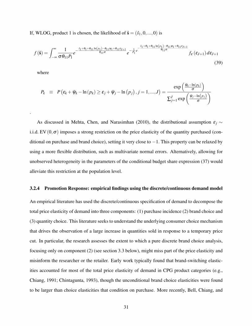
If, WLOG, product 1 is chosen, the likelihood of s = (s1,0, ...,0) is

f (s) =∫

∞

−∞

1σθ11P1

e−s1+θ1+θ11 ln(p1)−θ11ψ1+θ11εJ+1

θ11σ e−1

P1e−

s1+θ1+θ11 ln(p1)−θ11ψ1+θ11εJ+1θ11σ

fε (εJ+1)dεJ+1

(39)

where

Pk ≡ P(εk + ψk− ln(pk)≥ ε j + ψ j− ln

(p j), j = 1, ...,J

)=

exp(

ψk−ln(pk)σ

)∑

Jj=1 exp

(ψ j−ln(p j)

σ

).

As discussed in Mehta, Chen, and Narasimhan (2010), the distributional assumption ε j ∼

i.i.d. EV(0,σ) imposes a strong restriction on the price elasticity of the quantity purchased (con-

ditional on purchase and brand choice), setting it very close to−1. This property can be relaxed by

using a more flexible distribution, such as multivariate normal errors. Alternatively, allowing for

unobserved heterogeneity in the parameters of the conditional budget share expression (37) would

alleviate this restriction at the population level.

3.2.4 Promotion Response: empirical findings using the discrete/continuous demand model

An empirical literature has used the discrete/continuous specification of demand to decompose the

total price elasticity of demand into three components: (1) purchase incidence (2) brand choice and

(3) quantity choice. This literature seeks to understand the underlying consumer choice mechanism

that drives the observation of a large increase in quantities sold in response to a temporary price

cut. In particular, the research assesses the extent to which a pure discrete brand choice analysis,

focusing only on component (2) (see section 3.3 below), might miss part of the price elasticity and

misinform the researcher or the retailer. Early work typically found that brand-switching elastic-

ities accounted for most of the total price elasticity of demand in CPG product categories (e.g.,

Chiang, 1991; Chintagunta, 1993), though the unconditional brand choice elasticities were found

to be larger than choice elasticities that condition on purchase. More recently, Bell, Chiang, and

31

Padmanabhan (1999)’s empirical generalizations indicate that the relative role of the brand switch-

ing elasticity varies across product categories. On average, they find that the quantity decision

accounts for 25% of the total price elasticity of demand, suggesting that purchase acceleration ef-

fects may be larger than previously assumed. These results are based on static models in which

any purchase acceleration would be associated with an increase in consumption. In section 5.1, we

extend this discussion to models that allow for forward-looking consumers to stock-pile storable

consumer goods in anticipation of higher future prices.

3.3 Indivisibility and the Pure Discrete Choice Restriction in the Neoclassi-

cal Model

One of the most practical restrictions drawn from our empirical stylized facts in section 2 is pure

discrete choice behavior. In many product categories, the consumer purchases at most one unit

of a single product on a given trip. Discrete choice behavior also broadly applies to other non-

CPG product domains such as automobiles, computers and electronic devices. The pure discrete

choice model simplifies even our discrete product choice model in section 3.2 by eliminating the

intensive quantity choice margin and focusing solely on the discrete product choice decision. Not

surprisingly, pure discrete choice models have become extremely popular for modeling demand

both with the micro data and with more macro data that reports market shares that aggregate un-

derlying discrete choices. We now discuss the relationship between the classic pure discrete choice

models of demand estimated in practice (e.g. multinomial logit and probit) and contrast them to

the derivation of pure discrete choice from the neoclassical models derived above.

3.3.1 A Neoclassical Derivation of the Pure Discrete Choice Model of Demand

Recall from section 3 where we defined the neoclassical economic model of consumer choice

based on the following utility maximization problem:

V (p,y;θ ,ε)≡ maxx

{U (x;θ ,ε) : x′p 6 y, x≥ 0

}(40)

32

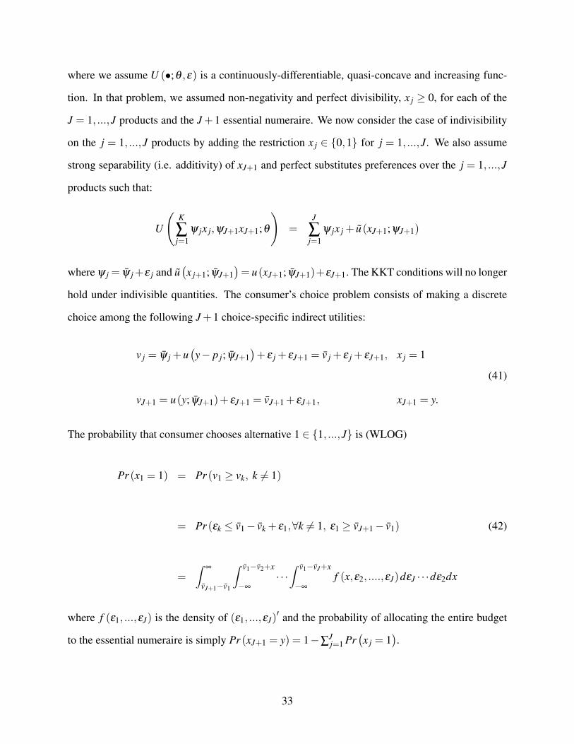
where we assume U (•;θ ,ε) is a continuously-differentiable, quasi-concave and increasing func-

tion. In that problem, we assumed non-negativity and perfect divisibility, x j ≥ 0, for each of the

J = 1, ...,J products and the J +1 essential numeraire. We now consider the case of indivisibility

on the j = 1, ...,J products by adding the restriction x j ∈ {0,1} for j = 1, ...,J. We also assume

strong separability (i.e. additivity) of xJ+1 and perfect substitutes preferences over the j = 1, ...,J

products such that:

U

(K

∑j=1

ψ jx j,ψJ+1xJ+1;θ

)=

J

∑j=1

ψ jx j + u(xJ+1;ψJ+1)

where ψ j = ψ j+ε j and u(x j+1; ψJ+1

)= u(xJ+1; ψJ+1)+εJ+1. The KKT conditions will no longer

hold under indivisible quantities. The consumer’s choice problem consists of making a discrete

choice among the following J+1 choice-specific indirect utilities:

v j = ψ j +u(y− p j; ψJ+1

)+ ε j + εJ+1 = v j + ε j + εJ+1, x j = 1

vJ+1 = u(y; ψJ+1)+ εJ+1 = vJ+1 + εJ+1, xJ+1 = y.

(41)

The probability that consumer chooses alternative 1 ∈ {1, ...,J} is (WLOG)

Pr (x1 = 1) = Pr (v1 ≥ vk, k 6= 1)

= Pr (εk ≤ v1− vk + ε1,∀k 6= 1, ε1 ≥ vJ+1− v1) (42)

=∫

∞

vJ+1−v1

∫ v1−v2+x

−∞

· · ·∫ v1−vJ+x

−∞

f (x,ε2, ....,εJ)dεJ · · ·dε2dx

where f (ε1, ...,εJ) is the density of (ε1, ...,εJ)′ and the probability of allocating the entire budget

to the essential numeraire is simply Pr (xJ+1 = y) = 1−∑Jj=1 Pr

(x j = 1

).

33

If we assume (ε1, ...,εJ)′ ∼ i.i.d. EV (0,1), the choice probabilities in (42) become

Pr (x1 = 1) = exp(ψ1+u(y−p1;ψJ+1))

∑Jk=1 exp(ψk+u(y−pk;ψJ+1))

[1− e

(−e(−u(y;ψJ+1))∑

Jk=1 e(ψk+u(y−pk ;ψJ+1))

)]

Prob(xJ+1 = y) =[

1− e(−e(−u(y;ψJ+1))∑

Jk=1 e(ψk+u(y−pk ;ψJ+1))

)].

(43)

Suppose the researcher has a data sample with i = 1, ...,N independent consumer purchase obser-

vations. A maximum likelihood estimator of the model parameters can be constructed as follows:

L (θ |y) =N

∏i=1

J

∏j=1

Pr (xJ+1 = y)yiJ+1 Pr(x j = 1

)yi j (44)

where yi j indicates whether observation i resulted in choice alternative j, and θ = (ψ1, ..., ψJ+1)′ .

While the probabilities (43) generate a tractable maximum likelihood estimator based on (44),

the functional forms do not correspond to the familiar multinomial logit specification used through-

out the literature on discrete choice demand McFadden (e.g., 1981)18. To understand why the

neoclassical models from earlier sections do not nest the usual discrete choice models, note that

the random utilities εJ+1 “difference out” in (42) and the the model is equivalent to a deterministic

utility for the decision to allocate the entire budget to the numeraire. This result arises because

of the adding-up condition associated with the budget constraint, which we resolved by assuming

x∗J+1 > 0, just as we did in section 3 above.

Lee and Allenby (e.g., 2014) extend the pure discrete choice model to allow for multiple dis-

crete choice and indivisible quantities for each product. As before, assume there are j = 1, ...,J

products and a J + 1 essential numeraire. To address the indivisibility of the j = 1, ...,J prod-

ucts, assume x j ∈ {0,1, ...} for j = 1, ...,J. If utility is concave, increasing and additive19, U (x) =

∑Jj=1 u j

(x j)+αJ+1 (xJ+1), the consumer’s decision problem consists of selecting an optimal quan-

18Besanko, Perry, and Spady (1990) study the monopolistic equilibrium pricing and variety of brands supplied in amarket with discrete choice demand of the form 43.

19The tractability of this problem also requires assuming linearity in the essential numeraire u(xJ+1) = α (xJ+1) sothat the derivation of the likelihood can be computed separately for each product alternative.

34

tity for each of the products and the essential numeraire, subject to her budget constraint. Let

F ={(x1, ...,xJ) |y−∑ j x j p j ≥ 0, x j ∈ {0,1, ...}

}be the set of feasible quantities that satisfy the

consumer’s budget constraint, where xJ+1 = y−∑ j x j p j. The consumer picks an optimal quantity

vector x∗ ∈ F such that U (x∗)≥U (x) ∀x ∈ F.

To derive a tractable demand solution, Lee and Allenby (2014) assume that utility has the

following form20:

u j (x) =α j exp

(ε j)

γ jlog(γ jx+1

).

The additive separability assumption is critical since it allows the optimal quantity of each brand

to be determined separately. In particular, for each j = 1, ...,J the optimality of x∗j is ensured if

U(

x∗1, ...,x∗j , ...,x

∗J

)≥max

{U(

x∗1, ...,x∗j +∆, ...,x∗J

)|x∗ ∈ F, ∆ ∈ {−1,1}

}. The limits of integra-

tion of the utility shocks, ε , can therefore be derived in closed form:

fx (x;θ) =J

∏j=1

∫ ub j

lb j

fε

(ε j)

dε j

where lb j = log(

αJ+1 p jγ jα j

)−log

(log(

γ j x j+1γ j(x j−1)+1

))and ub j = log

(αJ+1 p jγ j

α j

)−log

(log(

γ j(x j+1)+1γ j x j+1

)).

3.3.2 The Classic Pure Discrete Choice Model of Demand

Suppose as before that the consumer makes a discrete choice between each of the products in

the commodity group. We again assume a bivariate utility over an essential numeraire and a

commodity group, with perfect substitutes over the j = 1, ...,J products in the commodity group:

U(

∑Jj=1 ψ jx j,xJ+1

). If we impose indivisibility on the product quantities such that x j ∈ {0,1},

20This specification is a special case of the translated CES model desribed earlier when the satiation parameterasymptotes to 0 (e.g., Bhat, 2008).

35

the choice problem once again becomes a discrete choice among the j = 1, ...,J+1 alternatives

v j =U(ψ j,y− p j

)+ ε j, j = 1, ...,J

vJ+1 =U (0,y)+ εJ+1.

(45)

In this case, the random utility εJ+1 does not “difference out” and hence we will end up with a

different system of choice probabilities. If we again assumes that (ε1, ...,εJ+1) ∼ i.i.d. EV(0,1),

the corresponding choice probabilities have the familiar multinomial logit (MNL) form:

Pr ( j) = Prob(v j ≥ vk, for k 6= j

)

=exp(U(ψ j,y−p j))

exp(U(0,y))+∑Jk=1 exp(U(ψk,y−pk))

.

(46)

Similarly, assuming (ε1, ...,εJ+1)∼ N (0,Σ) would give rise to the standard multinomial probit.

We now examine why we did not obtain the same system of choice probabilities as in the

previous section. Unlike the derivation in the previous section, the random utilities in (45) were

not specified as primitive assumptions on the underlying utility function U(

∑Jj=1 ψ jx j,xJ+1

). In-

stead, they were added on to the choice-specific values. An advantage of this approach is that it

allows the researcher to be more agnostic about the exact interpretation of the errors. In the econo-

metrics literature, ε are interpreted as unobserved product characteristics, unobserved utility or

tastes, measurement error or specification error. However, the probabilistic choice model has also

been derived by mathematical psychologists (e.g., Luce, 1977) who interpret the shocks as psy-

chological states, leading to potentially non-rational forms of behavior. Whereas econometricians

interpret the probabilistic choice rules in (46) as the outcome of utility maximization with random

utility components, mathematical psychologists interpret (46) as stochastic choice behavior (see

the discussion in Anderson, de Palma, and Thisse, 1992, chapters 2.4 and 2.5). A more recent

literature has derived the multinomial logit from a theory of “rational inattention.” Under rational

inattention, the stochastic component of the model captures a consumer’s product uncertainty and

36

the costs of endogenously reducing uncertainty through search (e.g., Matejka and McKay, 2015;

Joo, 2018).

One approach to rationalize the system 46 is to include an additional non-market good, j =

0, with price p0 = 0 in the consumer’s choice set, usually defined as “home production” (e.g.,

Anderson and de Palma, 1992): U(

∑Jj=0 ψ jx j,xJ+1

). In this case, we define the commodity group

of interest as an essential good and the decision not to purchase any of the market goods implies

the choice of home production of the commodity. The choice-specific values correspond exactly

to 45 and the shock εJ+1 is now interpreted as the random utility from home production. We do

not include a deterministic component to home production since it is unobserved to the researcher.

However, note once again that this model is different from the neoclassical models discussed in

sections 3 and 3.2 because we have now included an additional non-market good representing

household production.

The MNL was first applied to marketing panel data for individual consumers by Guadagni and

Little (1983). The linearity of the conditional indirect utility function explicitly rules out income

effects in the substitution patterns between the inside goods. We discuss tractable specifications

that allow for income effects in section 4.1 below. If income is observed, then income effects in the

substitution between the the commodity group and the essential numeraire can be incorporated by

allowing for non-linearity in the utility of the numeraire. For instance, if U (xJ+1) = ψJ+1 ln(xJ+1)

then we get choice probabilities21

Pr (k;θ) =exp(ψk +ψJ+1 ln(y− pk))

exp(ψJ+1 ln(y))+∑Jj=1 exp

(ψ j +ψJ+1 ln

(y− p j

)) . (47)

This specification also imposes an affordability condition by excluding any alternative for which

p j > y.

The appeal of the MNL’s closed-form specification comes at a cost for demand analysis. If

U (xJ+1) = ψJ+1xJ+1 as is often assumed in the literature, the model exhibits the well-known

21We can derive this specification from the assumption of Cobb-Douglas utility: U (x1, ...,xJ+1;θ) =

exp(

∑J+1j=1 ψ jx j

)xψJ+1

J+1 .

37

Independence of Irrelevant Alternatives property. The IIA property can impose unrealistic substi-

tution patterns in demand analysis. At the individual consumer level, the cross-price elasticity of

demand is constant:∂Pr ( j)

∂ pk

pk

Pr ( j)= ψJ+1Pr (k) pk

so that substitution patterns between products will be driven by their prices and purchase frequen-

cies, regardless of attributes. Moreover, a given product competes uniformly on price with all other

products. One solution is to use a non-IIA specification. For instance, error components variants of

the extreme value distribution, like nested logit and the generalized extreme value distribution, can

relax the IIA property within pre-determined groups of products (e.g., McFadden, 1981; Cardell,

1997)22. If we instead assume that ε ∼ N (0,Σ) with appropriately scaled covariance matrix Σ,

we obtain the multinomial probit (e.g., McCulloch and Rossi, 1994; Goolsbee and Petrin, 2004).

Dotson, Howell, Brazell, Otter, Lenk, MacEachern, and Allenby (2015) parameterize the covari-

ance matrix, Σ, using product characteristics to allow for a scalable model with correlated utility

errors and, hence, stronger substitution between similar products. When consumer panel data are

available, another solution is to use a random coefficients specification that allows for more flexible

aggregate substitution patterns (see Chapter 2 of this volume).

In their seminal application of the multinomial logit to consumer-level scanner data, Guadagni

and Little (1983) estimated demand for the ground coffee category using 78 weeks of transaction

data for 2,000 households shopping in 4 Kansas City Supermarkets. Interestingly, they found that

brand and pack size were the most predictive attributes for consumer choices. They also included

the promotional variables “feature ad” and “in-aisle display” as additive utility shifters. These

variables have routinely been found to be predictive of consumer choices. However, the structural

interpretation of a marginal utility from a feature ad or a display is ambiguous. While it is possible

that consumers obtain direct consumption value from a newspaper ad or a display, it seems more

likely that these effects are the reduced-form of some other process such as information search.

22Misra (2005) shows that the disutility minimization formulation of the multinomial logit (or “reverse logit”) leadsto a different functional form of the choice probabilities that does not exhibit the IIA property.

38

Exploring the structural foundations of the “promotion effects” remains a fruitful area for future

research.

4 Some Extensions to the Typical Neoclassical Specifications

4.1 Income Effects

Most of the empirical specifications discussed earlier imposed regularity conditions that, as a

byproduct, impose strong restrictions on the income effects on demand. Since the seminal work by

Engel (1857), the income elasticity of demand has been used to classify goods based on consump-

tion behavior. Goods with a positive income elasticity are classified as Normal goods, for which

consumers increase their consumption as income increases. Goods with a negative income elas-

ticity are classified as Inferior goods, for which consumers decrease their consumption as income

increases. Engel’s law is based on the empirical observation that households tend to allocate a

higher proportion of their income to food as they become poorer (e.g., Engel, 1857). Accordingly,

we define necessity goods and luxury goods based on whether the income elasticity of demand is

less than or greater than one. Homothetic preferences restrict all products to be strict Normal goods

with an income elasticity of one, thereby limiting the policy implications one can study with the

model. Quasi-linear preferences over the composite “outside” good restrict the income elasticity

to zero, eliminating income effects entirely.

When the empirical focus is on a specific product category for a low-priced item like a CPG

product, it may be convenient to assume that income effects are likely to be small and inconse-

quential23. This assumption is particularly convenient when a household’s income or shopping

budget is not observed. However, overly restrictive income effects can limit a model’s predicted

substitution patterns, leading to potentially adverse policy implications (see McFadden’s forward

to Anderson, de Palma, and Thisse (1992) for a discussion). Even when a household’s income is

23Income effects are typically incorporated into demand analyses of high-priced, durable consumption goods likeautomobiles (e.g., Berry, Levinsohn, and Pakes, 1995).

39

static, large changes in relative prices could nevertheless create purchasing power effects. Con-

sider the bivariate utility function specification with perfect substitutes in the focal commodity

group from section 3.2: U(

∑Jj=1 ψ jx j,xJ+1

). For the products in the first commodity group, con-

sumers will select the product k where pkψk≤ p j

ψ jfor all j 6= k. When consumers face the same

prices and have homogeneous quality perceptions, they would all be predicted to choose the same

product. Changes in a consumer’s income would change the relative proportion of income spent

on the commodity group and the essential numeraire. But the income change would not affect

her choice of product. Therefore, homotheticity may be particularly problematic in vertically dif-

ferentiated product categories where observed substitution patterns may be asymmetric between

products in different quality tiers. For instance, the cross-elasticity of demand for lower-quality

products with respect to premium products’ prices may be higher than the cross-elasticity of de-

mand for higher-quality products with respect to the lower-quality products’ prices (e.g., Blattberg

and Wisniewski, 1989; Pauwels, Srinivasan, and Franses, 2007). Similarly, Deaton and Muell-

bauer (1980b, p. 262) observed a cross-sectional income effect: “richer households systematically

tend to buy different qualities than do poorer ones.” Gicheva, Hastings, and Villas-Boas (2010)

found a cross-time income effect by showing that lower-income households responded to higher

gasoline prices by substituting their grocery purchases towards promotional-priced items, which

could be consistent with asymmetric switching patterns if lower-quality items are more likely to

be promoted. Similarly, Ma, Ailawadi, Gauri, and Grewal (2011) found that households respond

to increases in gasoline prices by substituting from national brands to lower-priced brands and

to unadvertised own brands supplied by retailers, or “private labels.” These substitution patterns

suggest that national brands are normal goods24.

4.1.1 A Non-Homothetic Discrete Choice Model

Given the widespread use of the pure discrete choice models, like logit and probit, we now discuss

how to incorporate income effects into these models without losing their empirical tractability.

24Although, Dubé, Hitsch, and Rossi (2017) find highly income-inelastic demand for private label CPGs identifiedoff the large household income shocks during the Great Recession.

40

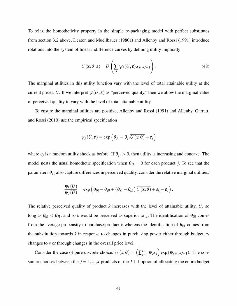
To relax the homotheticity property in the simple re-packaging model with perfect substitutes

from section 3.2 above, Deaton and Muellbauer (1980a) and Allenby and Rossi (1991) introduce

rotations into the system of linear indifference curves by defining utility implicitly:

U (x;θ ,ε) = U

(∑

jψ j (U ,ε)x j,xJ+1

). (48)

The marginal utilities in this utility function vary with the level of total attainable utility at the

current prices, U . If we interpret ψ (U ,ε) as “perceived quality,” then we allow the marginal value

of perceived quality to vary with the level of total attainable utility.

To ensure the marginal utilities are positive, Allenby and Rossi (1991) and Allenby, Garratt,

and Rossi (2010) use the empirical specification

ψ j (U ,ε) = exp(

θ j0−θ j1U (x;θ)+ ε j

)

where ε j is a random utility shock as before. If θ j1 > 0, then utility is increasing and concave. The

model nests the usual homothetic specification when θ j1 = 0 for each product j. To see that the

parameters θ j1 also capture differences in perceived quality, consider the relative marginal utilities:

ψk (U)

ψ j (U)= exp

(θk0−θ j0 +

(θ j1−θk1

)U (x;θ)+ εk− ε j

).

The relative perceived quality of product k increases with the level of attainable utility, U , so

long as θk1 < θ j1, and so k would be perceived as superior to j. The identification of θk0 comes

from the average propensity to purchase product k whereas the identification of θk1 comes from

the substitution towards k in response to changes in purchasing power either through budgetary

changes to y or through changes in the overall price level.

Consider the case of pure discrete choice: U (x;θ) =(

∑J+1j=1 ψ jx j

)exp(ψJ+1xJ+1). The con-

sumer chooses between the j = 1, ...,J products or the J +1 option of allocating the entire budget

41

to the outside good with the following probabilities:

Pr (k;θ) =exp(θk0−θk1Uk−ψJ+1 p j

)1+∑

Jj=1 exp

(θ j0−θ j1U j−ψJ+1 p j

)where Uk is solved numerically as the solution to the implicit equation

ln(

Uk)= θk0−θk1Uk−ψJ+1 p j. (49)

Maximum likelihood estimation will therefore nest the fixed-point calculation to (49) at each stage

of the parameter search.

In their empirical case study of margarine purchases, Allenby and Rossi (1991) find that the de-

mand for generic margarine is considerably more elastic in the price of the leading national brand

than vice versa. This finding is consistent with the earlier descriptive findings regarding asym-

metric substitution patterns, the key motivating fact for the non-homothetic specification. Allenby,

Garratt, and Rossi (2010) project the brand intercepts and utility rotation parameters, θ j0 and θ j1

respectively, onto advertising to allow the firms’ marketing efforts to influence the perceived su-

periority of their respective brands. In an application to survey data from a choice-based conjoint

survey with a randomized advertising treatment, they find that ads change the substitution patterns

in the category by causing consumers to allocate more spending to higher-quality goods.

4.2 Complementary Goods

The determination of demand complementarity figured prominently in the consumption litera-

ture (see the survey by Houthakker, 1961). But, the microeconometric literature tackling demand

with corner solutions has frequently used additive models that explicitly rule out complementarity

and assume products are strict substitutes (Deaton and Muellbauer, 1980b, pages 138-139). For

many product categories, such as laundry detergents, ketchups, and refrigerated orange juice, the

assumption of strict substitutibility seems reasonable for most consumers. However, in other prod-

42

uct categories where consumers purchase large assortments of flavors or variants, such as yogurt,

carbonated soft drinks, beer and breakfast cereals, complementarity may be an important part of

choices. For a shopping basket model that accounts for the wide array of goods, complementarity

seems quite plausible between broader commodity groups (e.g. pasta and pasta sauce, or cake mix

and frosting).

Economists historically defined complementarity based on the supermodularity of the utility

function and the increasing differences in utility associated with joint consumption. Samuelson

(1974) provides a comprehensive overview of the arguments against such approaches based on

the cardinality of utility. Chambers and Echenique (2009) formally prove that supermodularity is

not testable with data on consumption expenditures. Accordingly, most current empirical research

defines complementarity based on demand behavior, rather than as a primitive assumption about

preferences25.

Perhaps the most widely-cited definition of complementarity comes from Hicks and Allen

(1934) using compensated demand:

Definition 1. We say that goods j and k are complements if an increase in the price of j leads to a

decrease in the compensated demand for good k, substitutes if an increase in the price of j leads to

a increase in the compensated demand for good k, independent if an increase in the price of j has

no effect on the compensated demand for good k.

This definition has several advantages including symmetry and the applicability to any number

of goods. However, compensated demand is unlikely to be observed in practice. Most empirical

research tests for gross complementarity, testing for the positivity of the cross-derivatives of Mar-

shallian demands with respect to prices. The linear indifference curves used in most pure discrete

choice models eliminates any income effects, making the two definitions equivalent. A recent

literature has worked on establishing the conditions under which an empirical test for complemen-

tarity is identified with standard consumer purchase data (e.g., Samuelson, 1974; Gentzkow, 2007;

25An exception is Lee, Kim, and Allenby (2013) who use a traditional definition of complementarity based on thesign of the cross-partial derivative of utility.

43

Chambers, Echenique, and Shmaya, 2010).

The definition of complementarity based on the cross-price effects on demand can be prob-

lematic in the presence of multiple goods. Samuelson (1974, p. 1255) provides the following

example:

... sometimes I like tea and cream... I also sometimes take cream with my coffee.

Before you agree that cream is therefore a complement to both tea and coffee, I should

mention that I take much less cream in my cup of coffee than I do in my cup of tea.

Therefore, a reduction in the price of coffee may reduce my demand for cream, which

is an odd thing to happen between so-called complements.

To see how this could affect a microeconometric test, consider the model of bivariate utility over

a commodity group defined as products in the coffee and cream categories, and an essential nu-

meraire that aggregates expenditures on all other goods (including tea). Even with flexible substi-

tution patterns between coffee and cream, empirical analysis could potentially produce a positive

estimate of the cross-price elasticity of demand for cream with respect to the price of coffee if

cream is more complementary with tea than with coffee.

On the one hand, this argument highlights the importance of multi-category models, like the

ones we will discuss in section 4.2.2 below, that consider both the intra-category and inter-category

patterns of substitution. For instance, one might specify a multivariate utility over all the beverage-

related categories and the products within each of the categories. The multi-category model would

characterize all the direct and indirect substitution patterns between goods Ogaki (1990, p. 1255).

On the other hand, a multi-category model increases the technical and computational burden of de-

mand estimation dramatically. As discussed in Gentzkow (2007, p. 720), the estimated quantities

in the narrower, single-category specification should be interpreted as “conditional on the set of al-

ternative goods available in the market.” The corresponding estimates will still be correct for many

marketing applications, such as the evaluation of the marginal profits of a pricing or promotional

decision. The estimates will be problematic if there is a lot of variation in the composition of the

numeraire that, in turn, changes the specification of utility for the commodity group of interest.

44

Our discussion herein focuses on static theories of complementarity. While several of the

models in section 3 allow for complementarity, the literature has been surprisingly silent on the

identification strategies for testing complementarity. An exception is Gentzkow (2007), which

we discuss in more detail below. A burgeoning literature has also studied the complementarities

that arise over time in durable goods markets with inter-dependent demands and indirect network

effects. These “platform markets” include such examples as the classic “razors & blades” and

“hardware & software” cases (e.g., Ohashi, 2003; Nair, Chintagunta, and Dubé, 2004; Hartmann

and Nair, 2010; Lee, 2013; Howell and Allenby, 2017).

4.2.1 Complementarity Between Products Within a Commodity Group

In most marketing models of consumer demand, products within a commodity group are assumed

to be substitutes. When a single product in the commodity group is purchased on a typical trip, the

perfect substitutes specification is used (see sections 3.2 and 3.3). However, even when multiple

products are purchased on a given trip, additive models that imply products are strict substitutes are

still used (see for instance the translated CES model in section 3.1.4). Even though some consumer

goods products are purchased jointly, they are typically assumed to be consumed separately. There

are of course exceptions. The ability to offer specific bundles of varieties of beverage flavors or

beer brands could have a complementary benefit when a consumer is entertaining guests. Outside

the CPG domain, Gentzkow (2007) analyzed the potential complementarities of jointly consuming

digital and print versions of news.

To incorporate the definition of complementary goods into our demand framework, we begin

with a discrete quantity choice model of utility over j = 1, ...,J goods in a commodity group,

where x j ∈ {0,1}, and a J + 1 essential numeraire. The goal consists of testing for complemen-

tarity between the goods within a given commodity group. The discussion herein closely follows

Gentzkow (2007).

We index all the possible commodity-group bundles the consumer could potentially purchase

as c ∈P ({1, ...,J}), using c = 0 to denote the allocation of her entire budget to the numeraire.

45

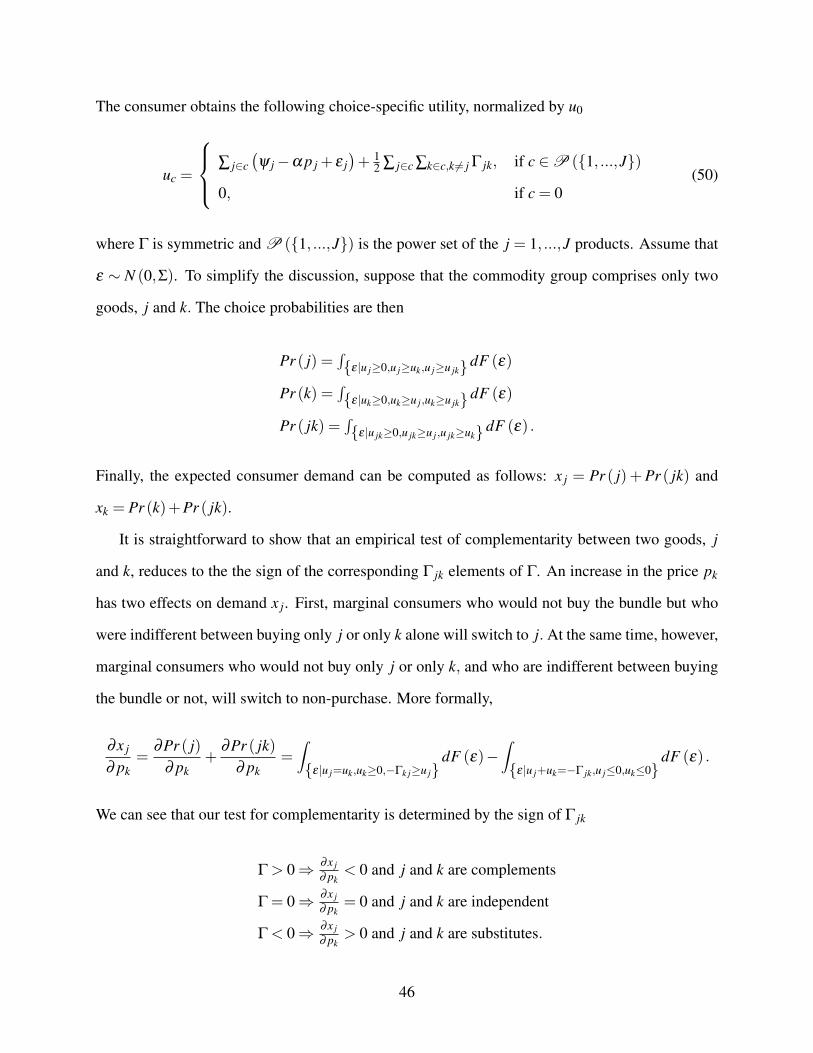
The consumer obtains the following choice-specific utility, normalized by u0

uc =

∑ j∈c(ψ j−α p j + ε j

)+ 1

2 ∑ j∈c ∑k∈c,k 6= j Γ jk, if c ∈P ({1, ...,J})

0, if c = 0(50)

where Γ is symmetric and P ({1, ...,J}) is the power set of the j = 1, ...,J products. Assume that

ε ∼ N (0,Σ). To simplify the discussion, suppose that the commodity group comprises only two

goods, j and k. The choice probabilities are then

Pr ( j) =∫{ε|u j≥0,u j≥uk,u j≥u jk} dF (ε)

Pr (k) =∫{ε|uk≥0,uk≥u j,uk≥u jk} dF (ε)

Pr ( jk) =∫{ε|u jk≥0,u jk≥u j,u jk≥uk} dF (ε) .

Finally, the expected consumer demand can be computed as follows: x j = Pr ( j)+Pr ( jk) and

xk = Pr (k)+Pr ( jk).

It is straightforward to show that an empirical test of complementarity between two goods, j

and k, reduces to the the sign of the corresponding Γ jk elements of Γ. An increase in the price pk

has two effects on demand x j. First, marginal consumers who would not buy the bundle but who

were indifferent between buying only j or only k alone will switch to j. At the same time, however,

marginal consumers who would not buy only j or only k, and who are indifferent between buying

the bundle or not, will switch to non-purchase. More formally,

∂x j

∂ pk=

∂Pr ( j)∂ pk

+∂Pr ( jk)

∂ pk=∫{ε|u j=uk,uk≥0,−Γk j≥u j}

dF (ε)−∫{ε|u j+uk=−Γ jk,u j≤0,uk≤0}

dF (ε) .

We can see that our test for complementarity is determined by the sign of Γ jk

Γ > 0⇒ ∂x j∂ pk

< 0 and j and k are complements

Γ = 0⇒ ∂x j∂ pk

= 0 and j and k are independent

Γ < 0⇒ ∂x j∂ pk

> 0 and j and k are substitutes.

46

Gentzkow (2007) provides a practical discussion of the identification challenges associated

with Γ jk, even for this stylized discrete choice demand system. At first glance, (50) looks like

a standard discrete choice model where each of the possible permutations of products has been

modeled as a separate choice26. But, the correlated error structure in ε plays an important role

in the identification of the complementarity. The key moment for the identification of Γ is the

incidence of joint purchase of products j and k, Pr ( jk) . But, high Pr ( jk) could arise either through

a high value of Γ jk or a high value of cov(ε j,εk

). A restricted covariance structure like logit, which

sets cov(ε j,εk

)= 0 will be forced to attribute a high Pr ( jk) to complementarity.

An ideal instrument for testing complementarity would be an exclusion restriction. Consider

for instance a variable z j that shifts the the mean utility for j but does not affect Γ or the mean

utility of good k. In the CPG context, the access to high-frequency price variation in all the ob-

served products as well as point-of-purchase promotional variables are ideal for this purpose. The

identification of Γ could then reflect the extent to which changes in z j affect demand xk.

Panel data can also be exploited to identify Γ jk and cov(ε j,εk

). Following the conventions in

the literature allowing for persistent, between-consumer heterogeneity, we could let ε be persistent,

consumer-specific “random effects.” We could then also include i.i.d. shocks that vary across time

and product to explain within-consumer switches in behavior. If joint purchase reflects cov(ε j,εk

),

we would expect to see some consumers frequently buying both and other consumers frequently

buying neither. But, conditional on a consumer’s average propensity to purchase either good, the

cross-time variation in choices should be uncorrelated. However, if joint purchase reflects Γ jk, we

would then expect more correlation over time whereby a consumer would either purchase both

goods or neither, but would seldom purchase only one of the two.

4.2.2 Complementarity Between Commodity Groups (multi-category models)

In the analysis of CPG data, most of the emphasis on complementarity has been between product

categories, where products within a commodity group are perceived as substitutes but different

26For instance, Manski and Sherman (1980) and Train, McFadden, and Ben-Akiva (1987) use logit and nested logitspecifications that restrict the covariance patterns in ε.

47

commodity groups may be perceived as complements. Typically, such cross-category models have

been specified using probabilistic choice models without a microeconomic foundation, and that

allow for correlated errors either in the random utility shocks (e.g., Manchanda, Ansari, and Gupta,

1999; Chib, Seetharaman, and Strijnev, 2002) or in the persistent heteroskedastic shocks associated

with random coefficients (e.g., Ainslie and Rossi, 1998; Erdem, 1998). For an overview of these

models, see the discussion in Seetharaman, Chib, Ainslie, Boatright, Chan, Gupta, Mehta, Rao,

and Strijnev (2005). The lack of a microfoundation complicates the ability to assign substantive

interpretations of model parameters. For instance, the identification discussion in the previous

section clarifies the fundamental distinction between correlated tastes (as in these multi-category

probabilistic models) and true product complementarity.

At least since Song and Chintagunta (2007), the empirical literature has used microfounded

demand systems to accommodate complementarity and substitutibility in the analysis of the com-

position of household shopping baskets spanning many categories during a shopping trip. Con-

ceptually, it is straightforward to extend the general, non-additive frameworks in section 3 to many

commodity groups. For instance, Bhat, Castro, and Pinjari (2015) introduce potential complemen-

tarity into the translated CES specification (see section 3.1.4) by relaxing additivity and allowing

for interaction effects27. In their study of the pro-competitive effects of mutiproduct grocery stores,

Thomassen, Seiler, Smith, and Schiraldi (2017) use a quadratic utility model that allows for gross

complementarity28. Mehta (2015) uses the indirect translog utility approximation to derive a multi-

category model that allows for complementarities.

The direct application of the models in section 3 and the extensions just discussed is limited by

the the escalation in parameters and the dimension of numerical integration, both of which grow

with the number of products studied. Typically, researchers have either focused their analysis

on a small set of product alternatives within a commodity group29 or have focused their analysis

27This specification does not ensure that global regularity is satisfied, which could limit the ability to conductcounterfactual predictions with the model.

28Empirically, they find that positive cross-price elasticities between grocery categories within a store are drivenmore by shopping costs associated with store choice than by intrinsic complementarities based on substitution patternsbetween categories.

29For instance, Wales and Woodland (1983) allow for J = 3 alternatives of meat: beef, lamb and other meat, and

48

on aggregate expenditure behavior across categories, collapsing each category into an aggregated

composite good 30. As we discuss in the next subsection, additional restrictions on preferences

have been required to accommodate product-level demand analysis across categories.

Example: Perfect Substitutes within a Commodity Group Suppose the consumer makes pur-

chase decisions across m = 1, ...,M commodity groups, each containing j = 1, ...,Jm products.

The consumer has a weakly separable, multivariate utility function over each of the M commodity

groups and an M + 1 essential numeraire good with price pM+1 = 1. Within each category, the

consumer has perfect substitutes sub-utility over the products, giving consumer utility

U

(J1

∑j=1

ψ1 jx1 j, ...,JM

∑j=1

ψM jxM j,ψM+1xM+1

)(51)

and budget constraintM

∑m=1

Jm

∑j=1

pm jxm j + xM+1 ≤ y.

The utility function is a generalization of the discrete choice specification in section 3.2 to many

commodity groups. At most, one product will be chosen in each of the M commodity groups. As

before, ψm j ≥ 0 and U () is continuously-differentiable, quasi-concave and increasing function in

each of its arguments. We also assume additional regularity conditions to ensure that an interior

quantity of the essential numeraire is always purchased, x∗M+1 > 0. This approach with perfect

substitutes within a category has been used in several studies (e.g., Song and Chintagunta, 2007;

Mehta, 2007; Lee and Allenby, 2009; Mehta and Ma, 2012). Most of the differences across studies

are based on the assumptions regarding the multivariate utility function U (x) .

Kim, Allenby, and Rossi (2002) allow for J = 6 brand alternatives of yogurt.30For instance, Kao, fei Lee, and Pitt (2001) look at expenditures across J = 7 food commodity groups, Mehta

(2015) looks at trip-level expenditures across J = 4 supermarket categories, and Thomassen, Seiler, Smith, and Schi-raldi (2017) look at trip-level expenditures across J = 8 supermarket product categories.

49

Lee and Allenby (2009) use a primal approach that specifies a quadratic utility over the com-

modity groups

U (u(x1;ψ1) , ...,u(xM;ψM) ,ψM+1xM+1)=M+1

∑m=1

βm0u(xm;ψm)−12

M+1

∑m=1

M+1

∑n=1

βmnu(xm;ψm)u(xn;ψn)

(52)

where

u(xm;ψm) =Jm

∑j=1

ψm jxm j

and

ψm j = exp(ψm j + εm j

).

where ψM+1 = 0, we normalize β10, and we assume symmetry such that βmn = βnm for m,n =

1, ...,M+1. The KKT conditions associated with the maximization of the utility function (52) are

now as follows:εm j = hm j (x∗;ψ) , i f x∗m j > 0

εm j ≤ hm j (x∗;ψ) , i f x∗m j = 0

where εm j = εm j − εM+1 and hm j (x∗;ψ) = − ln(

ψm jpm j

(βm0−∑

Mn=1 βmnu(x∗n;ψn)

)). Lee and Al-

lenby (2009) do not impose additional parameter restrictions to ensure the utility function is quasi-

concave, a sufficient condition for the coherency of the likelihood function. Instead, they set the

likelihood deterministically to zero at any support point where either the marginal utilities are neg-

ative or the utility function fails quasi-concavity31. While this approach may ensure coherency, it

will not ensure that global regularity is satisfied, which could limit the ability to conduct counter-

factual predictions with the model.

While products in the same commodity group are assumed to be perfect substitutes, the utility

function (52) allows for gross complementarity between a pair of commodity groups, m and n,

31The presence of indicator functions in the likelihood create discontinuities that could be problematic for maxi-mum likelihood estimation. The authors avoid this problem by using a Bayesian estimator that does not rely on thescore of the likelihood.

50

through the sign of the parameter βmn. In their empirical application, they find gross complemen-

tarity between laundry detergents and fabric softeners, which conforms with their intuition. All

other pairs of categories studied are found to be substitutes.

Song and Chintagunta (2007), Mehta (2007) and Mehta and Ma (2012) use a dual approach that

specifies a translog approximation of the indirect utility function. For simplicity of presentation,

we use the homothetic translog specification from Song and Chintagunta (2007)32

V (p,y;θ ,ε)= ln(y)−M+1

∑m=1

θm ln(

pm jm

ψm jm

)+

12

M+1

∑m=1

M+1

∑n=1

θmn ln(

pm jm

ψm jm

)ln(

pn jm

ψm jn

)+

M+1

∑m=1

ε jm ln(

pm jm

ψm jm

)(53)

where for each commodity group m, product jm satisfies ψm jmpm jm≥ ψm j

pm j, ∀ j 6= jm. To ensure the

coherency of the model, the following parameter restrictions are imposed:

∑m θm = 1, θmn = θnm, ∀m,n

∑M+1m=1 θmn = 0, ∀n.

Applying Roy’s identity, we derive the following conditional expenditure shares

sm jm (p,y;θ ,ε) = θm−M+1

∑n=1

θmn ln(

pm jm

ψm jm

). (54)

Since the homothetic translog approximation in (53) eliminates income effects from the expen-

diture shares, a test for complementarity between a pair of categories m and n amounts to testing

the sign of θmn. In particular, conditional on the chosen products in categories m and n, jm and jn

respectively, complementarity is identified off the changes in sm jmdue to the quality-adjusted price,pn jnψn jn

. Hence, several factors can potentially serve as instruments to test complementarity. Changes

in the price pn jn is an obvious source. In addition, if the perceived quality ψn jn is projected onto

observable characteristics of product jn, then independent characteristic variation in product jn

32Mehta and Ma (2012) use a non-homothetic translog approximation which generates a more complicated expen-diture share system, but which allows for more flexible income effects.

51

can also be used to identify the complementarity. The switching conditions will be important to

account for variation in the identity of the optimal product jn.

A limitation of this specification is that any complementarity only affects the intensive quantity

margin and does not affect the extensive brand choice and purchase incidence margins. Song and

Chintagunta (2007) do not detect evidence of complementarities in their empirical application,

which may be an artifact of the restricted way in which complementarity enters the model. Mehta

and Ma (2012) use a non-homothetic translog approximation that allows for complementarity in

purchase incidence as well as the expenditure shares. In their empirical application, they find strong

complementarities between the pasta and pasta sauces categories. These findings suggest that the

retailer should be coordinating prices across the two categories and synchronizing the timing of

promotional discounts.

4.3 Discrete Package Sizes and Non-Linear Pricing

In many consumer goods product categories, product quantities are restricted to the available pack-

age sizes. For instance, a customer must choose between specific pre-packaged quantities of liquid

laundry detergent (e.g., 32 oz, 64 oz or 128 oz) and cannot purchase an arbitrary, continuous quan-

tity. Early empirical work focused on brand choices, either narrowing the choice set to a specific

pack size or collapsing all the pack sizes into a composite brand choice alternative. However, these

models ignore the intensive quantity margin and limit the scope of their applicability to decision-

making on the supply side.

Firms typically offer an array of pre-packaged sizes as a form of commodity bundling, or

“non-linear pricing.” In practice, we expect to see quantity discounts whereby the consumer pays

a lower price-per-unit when she buys the larger pack size, consistent with standard second-degree

price discrimination (e.g., Varian, 1989; Dolan, 1987). However, several studies have documented

cases where firms use quantity-surcharging by raising the price-per-unit on larger pack sizes (e.g.,

Joo, 2018). The presence of nonlinear pricing introduces several challenges into our neoclassical

models of demand (e.g., Howell, Lee, and Allenby, 2016; Reiss and White, 2001). First, any kinks

52

in the pricing schedule will invalidate the use of the Kuhn-Tucker conditions33. Second, the dual

approach that derives demand using Roy’s identity is invalidated by non-linear pricing because

Roy’s Identity only holds under a constant marginal price for any given product. An exception is

the case of piecewise-linear budget sets (e.g., Hausman, 1985; Howell, Lee, and Allenby, 2016).

Third, the price paid per unit of a good depends on a consumer’s endogenous quantity choice,

creating a potential self-selection problem in addition to the usual non-negativity problem. To see

this potential source of bias, note that the consumer’s budget constraint is ∑ j p j(x j)

x j ≤ y, so

the price paid is endogenous as it will depend on unobservable (to the researcher) aspects of the

quantity demanded by the consumer.

4.3.1 Expand the Choice Set

One simple and popular modeling approach simply expands the choice set to include all available

combinations of brands and pack sizes (e.g., Guadagni and Little, 1983). A separate random utility

shock is then added to each choice alternative.

Suppose the consumer makes choices over the j = 1, ...,J products in a commodity group

where each product is available in a finite number of pre-packaged sizes, a ∈ A j. If the con-

sumer has additive preferences and the j = 1, ...,J products are perfect substitutes, U (x,xJ+1) =

u1

(∑

Jj=1 ψ jx j

)+u2 (xJ+1), her choice-specific indirect utilities are

v ja = u1(ψ jx ja

)+u2

(y− p ja

)+ ε ja, j = 1, ...,J, a ∈ A j

vJ+1 = u2 (y)+ εJ+1

(55)

where εa j ∼ i.i.d. EV (0,1), which allows for random perceived utility over the pack size variants

33See Lambrecht, Seim, and Skiera (e.g., 2007) and Yao, Mela, Chiang, and Chen (e.g., 2012) for the analysis ofdemand under three-part mobile tariffs.

53

of a given product. The probability of choosing pack size a for product k is then

Pr (ka;θ) =exp(u1 (ψkxka)+u2 (y− pka))

exp(u2 (y))+ ∑

{ j=1,..,J|a∈A j}exp(u1(ψ jx ja

)+u2

(y− p ja

)) . (56)

To see how one might implement this model in practice, assume the consumer has Cobb-Douglas

utility. In this case, u1 (ψkxka) = α1 ln(ψk) +α1 ln(xka) where α1 is the satiation rate over the

commodity group. Conceptually, this model could be expanded even further to allow the consumer

to purchase bundles of the products to configure all possible quantities that are feasible within the

budget constraint.

An important limitation of this specification is that it assigns independent random utility to each

pack size of the, otherwise, same product. This assumption would make sense if, for instance, a

large 64oz plastic bottle of soda is fundamentally different than a small, 12-oz aluminum can of

the same soda. In other settings, we might expect a high correlation in the random utility between

two pack-size variants of an otherwise identical product (e.g., 6 pack versus 12 pack of aluminum

cans of soda). Specifications that allow for such correlation within-brand, such as nested logit,

generalized extreme value or even multinomial probit could work. But, in a setting with many

product alternatives, it may not be possible to estimate the full covariance structure between each

of the product and size combinations.

In some settings, the temporal separation between choices can be used to simplify the problem.

For instance, Goettler and Clay (2011) and Narayanan, Chintagunta, and Miravete (2007) study

consumers’ discrete-continuous choices on pricing plan and usage. For instance, providers of mo-

bile data services and voice services typically offer consumers choices between pricing plans that

differ in their convexity. In practice, we might not expect the consumer to derive marginal utility

from the convexity of the pricing plan, seemingly rendering the pricing plan choice deterministic.

But, if the consumer makes a discrete choice between pricing plans in expectation of future us-

age choices, the expectation errors can be used as econometric uncertainty in the discrete choice

between plans.

54

4.3.2 Models of Pack Size Choice

Allenby, Shively, Yang, and Garratt (2004) use the following Cobb-Douglas utility specification

U (x,xJ+1) =J

∑j=1

∑a∈A j

α1 ln(ψ jxka

)+α2 ln

(y− p ja

)

where ψ j = exp(ψ j + ε j

)and ε j ∼ i.i.d. EV (0,1) . In this specification, the utilities of each of

the pack sizes for a given product are perfectly correlated. The corresponding, optimal pack size

choice for a given product j is deterministic:

a∗j = maxa∈A j

{α1 ln(xka)+α2 ln

(y− p ja

)}and does not depend on ψ j. The consumer’s product choice problem is then the usual maximization

across the random utilities of each of the j = 1, ...,J products corresponding to their respective

optimal pack sizes choices. The probability of observing the choice of product k is then

Pr (k;θ ,a∗) =exp(α1ψk +α1 ln(xak∗)+α2 ln(y− pak∗))

∑Jj=1 exp

(α1ψ j +α1 ln

(xa∗j

)+α2 ln

(y− pa∗j

)) (57)

where ak is the observed pack size chosen for brand k.

One limitation of the pack size demand specification (57) is that the corresponding likelihood

will not have full support. In particular, variation between pack sizes of a given brand, all else

equal, will reject the model. In a panel data version of the model with consumer-specific param-

eters, within-consumer switching between pack sizes of the same brand over time, all else equal,

would reject the model.

Goettler and Clay (2011) and Narayanan, Chintagunta, and Miravete (2007) propose a potential

solution to this issue, albeit in a different setting. The inclusion of consumer uncertainty over future

quantity needs allows for random variation in pack sizes.

55

5 Moving Beyond the Basic Neoclassical Framework

5.1 Stock-Piling, Purchase Incidence and Dynamic Behavior

The models discussed so far have treated the timing of purchase as a static consumer decision.

According to these models, a consumer allocates her entire budget to the essential numeraire (or

outside good), when all of the products’ prices exceed their corresponding reservation utilities, as

in equation (5) above. Indeed, the literature on price promotions has routinely reported a large

increase in sales during promotion weeks (see for instance the literature survey by Blattberg and

Neslin (1989) and the empirical generalizations in Blattberg, Briesch, and Fox (1995)).

However, in the case of storable products, consumers may accumulate an inventory and time

their purchases strategically based on their expectations about future price changes. An empirical

literature has found that price promotions affect both the quantity sold and the timing of purchases

through purchase acceleration (e.g., Blattberg, Eppen, and Lieberman, 1981; Scott A. Neslin and

Quelch, 1985; Gupta, 1991; Bell, Chiang, and Padmanabhan, 1999). This work estimates that

purchase acceleration accounts for between 14 and 50 percent of the promotion effect on quantities

sold. Purchase acceleration could simply reflect an increase in consumption. However, more recent

work finds that the purchase acceleration could reflect strategic timing based on price expectations.

Pesendorfer (2002) finds that while the quantity of ketchup sold is generally higher during periods

of low prices, the level depends on past prices. Hendel and Nevo (2006b) find that the magnitude

of the total sales response to a price discount in laundry detergent is moderated by the time since

the last price discount. The quantity sold increases by a factor of 4.7 if there was not a sale in

the previous week, but only by a factor of 2.0 if there was a sale in the previous week. Using

household panel data, Hendel and Nevo (2003) also detect a post-promotion dip in sales levels.

Looking across 24 CPG categories, Hendel and Nevo (2006b) find that households pay 12.7% less

than if they paid the average posted prices.

Collectively, these findings suggest that households may be timing their purchases strategically

to coincide with temporary price discounts. In this case, a static model of demand may over-

56

estimate the own-price response. The potential bias on cross-price elasticities is not as clear. In the

remainder of this section, we discuss structural approaches to estimate demand with stock-piling

and strategic purchase timing based, in part, on price expectations. These models can be used to

measure short and long-term price response through counterfactuals.

To the best of our knowledge, Blattberg, Buesing, Peacock, and Sen (1978) were the first to

propose a formal economic model of consumer stock-piling based on future price expectations. In

the spirit of Becker (1965)’s household production theory, they treat the household as a production

unit that maintains a stock of market goods to meet its consumption needs. While the estimation of

such a model exceeded the computing power available at that time, Blattberg, Buesing, Peacock,

and Sen (1978) find that observable household resources, such as home ownership, and shopping

costs, such as car ownership and dual-income status, are strongly associated with deal-proneness.

In the macroeconomics literature, Aguiar and Hurst (2007) extend the model to account for the

time allocation between “shopping” and “household production” to explain why older consumers

tend to pay lower prices (i.e. find the discount periods). In the following sub-sections, we discuss

more recent research that has estimated the underlying structure of a model of stock-piling.

5.1.1 Stock-Piling and Exogenous Consumption

Erdem, Imai, and Keane (2003) build on the discrete choice model formulation as in section 3.3.

Let t = 1, ...,T index time periods. At the start of each time period, a consumer has inventory it of

a commodity and observes the prices pt . The consumer can endogenously increase her inventory

by purchasing quantities x jkt of each of the j products, where k ∈ {1, ...,K} indexes the discrete set

of available pack sizes. Denote the non-purchase decision as x0t = 0. Assume the consumer incurs

a shopping cost if she chooses to purchase at least one of the products: F (xt ;τ) = τI{∑Jj=1 x jt>0}.

Her total post-purchase inventory in period t is: i′t = it +∑Jj=1 x jt .

After making her purchase decision, the consumer draws an exogenous consumption need that

is unobserved to the analyst, ωt ∼ Fω (ω), and that she consumes from her inventory, i′t34. Her

34The consumer therefore makes purchase decisions in anticipation of her future expected consumption needs, asin Dubé (2004).

57

total consumption during period t is therefore ct = min(ωt , i′t) , which is consumed at a constant

rate throughout the period35. Assume also that the consumer is indifferent between the brands in

her inventory when she consumes the commodity and that she consumes each of them in constant

proportion: c jt =cti′t

i′jt .

If the consumer runs out of inventory before the end of the period, ωt > ct , she incurs a stock-

out cost SC (ωt ,ct ;λ )= λ0+λ1 (ωt− ct). The consumer also incurs an inventory carrying cost each

period based on the total average inventory held during the period. Her average inventory in period

t is it =

i′t− ωt

2 , ωt ≤ i′t

i′tωt

i′t2 , ωt > i′t

. Her total inventory carrying cost is given by IC (i′t ,ωt ;δ ) = δ0it +δ1i2t .

Assume the consumer has the following perfect substitutes consumption utility function each

period:

U(it , it , pt ,ωt ;θ

)= ∑

Jj=1 ψ jc jt +ψJ+1

(y−∑ j,k p jktx jkt−F (xt ;τ)−SC (ω t ,ct ;λ )− IC (i′t ,ωt ;δ )

)

=c(i′t ,ωt)

i′ti′t +ψJ+1

(y−∑ j,k p jkt−F (xt ;τ)−SC (ω t ,c(i′t ,ωt) ;λ )− IC (i′t ,ωt ;δ )

)(58)

where i′t ≡∑Jj=1 ψ ji′jt is the post-purchase quality-adjusted inventory, and where the shopping cost,

inventory carrying cost and stock-out cost have all been subsumed into the budget constraint. The

vector θ = (ψ1, ...,ψJ+1,λ0,λ1,δ0,δ1,τ0) contains all the model’s parameters.

The three state variables are summarized by st =(it , it , pt

). The inventory state variables evolve

as follows:it =

(it−1 +∑

Jj=1 x jt

)(1− ct

i′t

)it =

(it−1 +∑

Jj=1 ψ jx jt

)(1− ct

i′t

) .

Assume in addition that consumers’ price beliefs are known to the analyst and evolve according

to the Markov transition density36 pt+1 ∼ fp (pt+1|pt).37 Therefore, the state vector also follows a35Sun, Neslin, and Srinivasan (2003) use a data-based approach that measures the exogenous consumption need as

a constant consumption rate, based on the household’s observed average quantity purchased.36Typically, a rational expectations assumption is made and the price process, Fp (pt+1|pt), is estimated in a first

stage using the observed price series. An interesting exception is Erdem, Keane, Öncü, and Strebel (2005) who elicitconsumers’ subjective price beliefs through a consumer survey.

37In four CPG case studies, Liu and Balachander (2014) find that a proportional hazard model for the price pro-

58

Markov Process which we denote by the transition density fs(s′|s,x jk

).

The consumer’s purchase problem is dynamic since she can control her future inventory states

with her current purchase decision. Assuming the consumer discounts future utility at a rate β ∈

(0,1) , the value function associated with her purchase decision problem in state st is

v(st ,εt) = maxj,k

{v jk (st ;θ)+ ε jkt

}(59)

where ε jkt ∼ i.i.d.EV (0,1) is a stochastic term known to the household at time t but not to the

analyst. v jk (s) is the choice-specific value function associated with choosing product j and pack

size k in state s

v jk (s;θ) =∫

U (st ,ω;θ) fω (ω)dω +β

∫v(s′,ε)

fs(s′|s,x jk

)d(s′,ε). (60)

When the taste parameters θ are known, the value functions in (59) and (60) can be solved numer-

ically (see for instance Erdem, Imai, and Keane (2003) for technical details).

Suppose the researcher observes a consumer’s sequence of choices, x = (x1, ..., xT ). Condi-

tional on the state, s, the probability that the consumer’s optimal choice is product j and pack size

k has the usual multinomial logit demand form:

Pr(x jk|s;θ

)=

exp(v jk (s;θ)

)exp(v0 (s;θ))+∑

Jk=1 exp

(v jk (s;θ)

) , x jk ∈ {x11, ...,xJK} . (61)

To accommodate the fact that the two inventory state variables, i and i, are not observed, we

partition the state as follows: s = (p, s) where s =(i, i). Since we do not observe the initial val-

ues of s0, we have a classic initial conditions problem (Heckman, 1981). We resolve the initial

conditions problem by assuming there is a true initial state, s0, with density fs (s0;θ).

We can now derive the density associated with the consumer’s observed sequence of purchase

cess fits the price data better and leads to a better fit of the demand model when used to capture consumers’ priceexpectations.

59

decisions, x:

f (x;θ) =∫ ( T

∏t=1

∫∏j,k

Pr(x jk|pt , st ,ω, s0;θ

)I{x jk=xt} fω (ω)dω

)fs (s0;θ)ds0. (62)

Consistent estimates of the parameters θ can then be obtained via simulated maximum likelihood.

5.1.2 Stock-Piling and Endogenous Consumption

The model in the previous section assumed an exogenous consumption rate, which implies that any

purchase acceleration during a price discount period reflects stock-piling. Sun (2005), Hendel and

Nevo (2006a) and Liu and Balachander (2014) allow for endogenous consumption. This important

extension allows for two types of response to a temporary price cut. In addition to stock-piling,

consumers can potentially increase their consumption of the discounted product. We focus on

the formulation in Hendel and Nevo (2006a), which reduces part of the computational burden of

Erdem, Imai, and Keane (2003) by splitting the likelihood into a static and a dynamic component.

A key assumption is that consumers only value the brand at the time of purchase so that the op-

timal consumption decisions are independent of specific brands and depend only on the quantities

purchased. During period t, the consumer derives the following consumption utility38

U (ct +ωt , it ,pt ;θ) = u(ct +ωt ;γc)+∑Jj=1 ∑

Kk=1 I{x jkt>0}

{ψJ+1

(y− p jkt

)+ψ jk

}−C (it+1;λc)

(63)

where as before we index the products by j = 1, ...,J and the discrete pack sizes available by

k ∈ {1, ...,K}. u(c+ω;γc) is the consumption utility with taste parameters γc and ω ∼ Fω (ω) is a

random “consumption need” shock. The start of period inventory is it = it−1+∑ j ∑k x jkt−1−ct−1.

C (it+1;λc) is the inventory carrying cost with cost-related parameters λc. As before, x denotes

a purchase quantity (as opposed to consumption), and ΨJ+1 captures the marginal utility of the

38Hendel and Nevo (2006a) also allow for point-of-purchase promotional advertising, like feature ads and displays,to shift utility in their specification.

60

numeraire good.

The three state variables are summarized by st = (it ,pt ,ωt). Inventory evolves as follows:

it = it−1 +∑Jj=1 x jt−1− ct−1 .

In addition, consumers’ form Markovian price expectations: pt+1 ∼ Fp (pt+1|pt) . Unlike Erdem,

Imai, and Keane (2003), the consumption need ω ∼ Fω (ω) is a state variable. The state variables,

st , follow a Markov Process with transition density fs(s′|s,x jk

).

The value function associated with the consumer’s purchase decision problem during period t

is

v(st ,εt) = maxj,k

{v jk (st)+ ε jkt

}(64)

where st is the state in period t, ε jkt ∼ i.i.d.EV (0,1) is a stochastic term known to the household

at time t but not to the analyst, and v jk (s) is the choice-specific value function associated with

choosing product j and pack size k in state s

v jk (st) = ψJ+1(y− p jkt

)+ψ jk +M

(st ,x jk;θc

)(65)

where M(st ,x jk;θc

)=max

c

{u(c+ωt ;γc)−C (it+1;λc)+β

∫v(s′,ε) fs

(s′|s,x jk,c

)fε (ε)d (s′,ε)

}and θc are the consumption-related parameters.

Hendel and Nevo (2006a) propose a simplified three-step approach to estimating the model

parameters. The value function (64) can be simplified by studying Equation (65), which indicates

that consumption is only affected by the quantity purchased, not the specific brand chosen. In

a first step, it is straightforward to show that consistent estimates of the brand taste parameters,

ψ = (ψ1, ...,ψJ+1) can be obtained from the following standard multinomial logit model of brand

choice across all brands available in the pack size k:

Pr ( j|st ,k;ψ) =exp(ψJ+1

(y− p jkt

)+ψ jk

)∑i exp(ψJ+1 (y− pikt)+ψik)

.

61

In a second step, define the expected value of the optimal brand choice, conditional on pack

size, as follows:

ηkt = log

{∑

jexp(ψJ+1

(y− p jkt

)+ψ jk

)}. (66)

Using an idea from Melnikov (2013), assume that ηt−1 is a sufficient statistic for ηt so that

F (ηt |st−1) can be summarized by F (ηt |ηt−1). The size-specific inclusive values can then be

computed with the brand taste parameters, ψ , and equation (66) and then used to estimate the

distribution F (ηt |ηt−1).

In a third step, the quantity choice state can then be defined as st = (it ,ηt ,ωt), which reduces

dimensionality by eliminating any brand-specific state variables. The value function associated

with the consumer’s quantity decision problem can now be written in terms of these size-specific

“inclusive value” terms:

v(st ,εt) = maxc,k

{u(c+ωt ;γc)−C (it+1;λc)+ηkt +β∫

v(s′,ε) fs (s′|s,xk,c) fε (ε)d (s′,ε)} .

(67)

Similarly, the pack-size choice-specific value functions can also be written in terms of these size-

specific “inclusive value” terms:

vk (st) = ηkt +Mk (st ;θc) (68)

where Mk (st ;θc)=maxc{u(c+ωt ;γc)−C (it+1;λc)+β

∫v(s′,ε) fs (s′|s,xk,c) fε (ε)d (s′,ε)}. The

corresponding optimal pack size choice probabilities are then:

Pr (k|st ;θc) =exp(ηk +Mk (st ;θc))

∑i exp(ηi +Mi (st ;θc)).

62

The density associated with the consumer’s observed sequence of pack size decisions, x, is39:

f (x;θc) =∫ ∫ ( T

∏t=1

∫Pr (xt |st , s0;θc) fω (ω)dω

)fω (ω) fs (s0;θc)d (ω, s0) . (69)

Consistent estimates of the parameters θc can then be obtained via simulated maximum likeli-

hood. A limitation of this three-step approach is that it does not allow for persistent, unobserved

heterogeneity in tastes.

5.1.3 Empirical Findings with Stock-piling Models

In a case study of household purchases of Ketchup, Erdem, Imai, and Keane (2003) find that the

dynamic stock-piling model described above fits the data well in-sample, in particular the timing

between purchases. Using simulations based on the estimates, they find that a product’s sales-

response to a temporary price cut mostly reflects purchase acceleration and category expansion, as

opposed to brand switching. This finding is diametrically opposite to the conventional wisdom that

“brand switchers account for a significant portion of the immediate increase volume due to sales

promotion” (Blattberg and Neslin, 1989, p. 82). The cross-price elasticities between brands are

found to be quite small compared to those from static choice models; although the exact magnitude

is sensitive to the specification of the price process representing consumers’ expectations. They

find much larger cross-price elasticities in response to permanent price changes and conclude that

long-run price elasticities are likely more relevant to policy analysts who want to measure the

intensity of competition between brands.

In case studies of Packaged Tuna and Yogurt, Sun (2005) finds that consumption increases with

the level of inventory and decreases in the level of promotional uncertainty. While promotions do

lead to brand-switching, she also finds that they increase consumption. A model that assumes

exogenous consumption over-estimates the extent of brand switching.

In a case study of Laundry Detergents, Hendel and Nevo (2006a) focus on the long-run price

elasticities by measuring the effects of permanent price changes. They find that a static model39The initial conditions can be resolved in a similar manner as in Erdem, Imai, and Keane (2003).

63

generates 30% larger price elasticities than the dynamic model. They also find that the static

model underestimates cross-price elasticities. Some of the cross-price elasticities in the dynamic

model are more than 20 times larger than those from the static model. Finally, the static model

overestimates the degree of substitution to the outside good by 200%. Seiler (2013) builds on

Hendel and Nevo (2006a)’s specification by allowing consumers with imperfect price information

to search each period before making a purchase decision. In a case study of laundry detergent

purchases, Seiler (2013)’s parameter estimates imply that 70% of consumers do not search each

period. This finding highlights the importance of merchandizing efforts, such as in-store displays,

to help consumers discover low prices. In addition, by using deeper price discounts, a firm can

induce consumers to engage in more price search which can increase total category sales. This

increase in search offsets traditional concerns about inter-temporal cannibalization due to strategic

purchase timing.

5.2 The Endogeneity of Marketing Variables

The frameworks discussed thus far focus entirely on the demand side of the market. However,

many of the most critical demand-shifting variables at the point of purchase consist of marketing

mix variables such as prices and promotions, including merchandizing activities like temporary

discounts, in-aisle displays and feature advertising. If these marketing variables are set strategi-

cally by firms with more consumer information than the researcher, any resulting correlation with

unobserved components of demand could impact the consistency of the likelihood-based estimates

discussed thus far. In fact, one of the dominant themes in the empirical literature on aggregate de-

mand estimation consists of the resolution of potential endogeneity of supply-side variables (e.g.,

Berry, 1994; Berry, Levinsohn, and Pakes, 1995). While most of the literature has focused on

obtaining consistent demand estimates in the presence of endogenous prices, bias could also arise

from the endogeneity of advertising, promotions and other marketing variables40. Surprisingly

little attention has been paid to the potential endogeneity of marketing variables in the estimation

40For instance, Manchanda, Rossi, and Chintagunta (2004) address endogenous detailing levels across physicians.

64

of individual consumer level demand. In the remainder of this section, we focus on the endo-

geneity of prices even though many of the key themes would readily extend to other endogenous

demand-shifting variables41.

Suppose a sample of i = 1, ...,N consumers each makes a discrete choice among j = 1, ...,J

product alternatives and a J+1 “no purchase” alternative. Each consumer is assumed to obtain the

following conditional indirect utility from choice j :

Vi j = ψ j−α pi j + εi j

ViJ+1 = εi,J+1

where εi ∼ i.i.d. F (ε) and pi j is the price charged to consumer i for alternative j. Demand estima-

tion is typically carried out by maximizing the corresponding likelihood function:

L = ∏i

∏j

Pr ( j;θ)yi j (70)

where Pr ( j;θ) = Pr(Vi j ≥Vik, ∀k 6= j

)and y = (yi1, ...,yiJ+1) indicates which of the j = 1, ...,J+

1 products was chosen by consumer i.

If cov(

pi j,εi j)6= 0 then the maximum likelihood estimator θ MLE based on (70) may be incon-

sistent since the likelihood omits information about ε. In general, endogeneity can arise in three

ways (see Wooldridge, 2002, for example):

1. Simultaneity: Firms observe and condition on ε i when they set their prices

2. Self-Selection: Certain types of consumers systematically find the lowest prices

3. Measurement Error: The researcher observes a noisy estimate of true prices, pi j : pi j =

pi j +ηi j.

41In the empirical consumption literature, the focus has been more on the endogeneity of household incomes thanthe endogeneity of prices (see for instance Blundell, Pashardes, and Weber, 1993). Since the analysis is typically at thebroad commodity group level (e.g., food), the concern is that household budget shares are determined simultaneouslywith consumption quantities.

65

Most of the emphasis has been on simultaneity bias whereby endogeneity arises because of the

strategic pricing decisions by the firms. Measurement error is not typically discussed in the demand

estimation literature. However, many databases contain time-aggregated average prices rather than

the actual point-of-purchase price, which could lead to classical measurement error. To the best

of our knowledge, a satisfactory solution has yet to be developed for demand estimation with this

type of measurement error. In many marketing settings, endogeneity bias could also arise from

the self-selection of consumers into specific marketing conditions based on unobserved (to the

researcher) aspects of their tastes. For instance, unobserved marketing promotions like coupons

could introduce both measurement error and selection bias if certain types of consumers are sys-

tematically more likely to find/have a coupon and use it (Erdem, Keane, and Sun, 1999). Similarly,

Howell, Lee, and Allenby (2016) propose an approach to resolve the price self-selection bias asso-

ciated with consumers choosing between non-linear pricing contracts based on observable (to the

researcher) aspects of their total consumption needs. If consumers face incomplete information

about the choice set, then selection could arise from price search and the formation of consumers’

consideration sets (e.g., Honka, 2014). Finally, the potential self-selection of consumers into dis-

count and regular prices based on their unobserved (to the researcher) potential stock-piling behav-

ior during promotional periods in anticipation of future price increases could also bias preference

estimates (e.g., Erdem, Imai, and Keane, 2003; Hendel and Nevo, 2006a).

For the remainder of this discussion, we will focus on price endogeneity associated with the

simultaneity bias. Suppose that j = 1, ...,J consumer goods in a product category are sold in

t = 1, ...,T static, spot markets by single-product firms playing a Bertrand-Nash pricing game.

Typically, a market is a store-week since stores tend to set their prices at a weekly frequency and

most categories in the store are “captured markets” in the sense that consumers likely to not base

their store choices on each of the tens of thousands of prices charged across the products carried in

a typical supermarket. On the demand side, consumers make choices in each market t to maximize

66

their choice-specific utility

Vi jt = v j (wt ,pt ;θ)+ξ jt + εi jt

ViJ+1t = εi,J+1t

(71)

where we distinguish between the exogenous point-of-purchase utility shifters, wt , and the prices,

pt . In addition, we now specify a composite error term consisting of the idiosyncratic utility shock,

εi jt ∼ i.i.d.EV (0,1) , and the common shock, ξ jt ∼ i.i.d. Fξ (ξ ), to control for potential product- j

specific characteristics that are observed to the firms when they set prices, but not to the researcher

(Berry, 1994). Consumers have corresponding choice probabilities, Pr ( j;θ |wt ,pt ,ξ t) for each of

the j alternatives including the J + 1 no-purchase alternative. Price endogeneity arises when the

firms conditions on ξ when setting its prices and cov(pt ,ξ t) 6= 0.

A consistent and efficient estimator can be constructed by maximizing the following likelihood

L(θ |x) = ∏t

∫· · ·∫

∏i

∏j

Pr ( j;θ |wt ,pt ,ξ )yi jt fp (pt |ξ ) fξ (ξ )dξ1...dξJ.

In practice, the form of the likelihood of prices may not be known and ad hoc assumptions about

fp (p|ξ ) could lead to additional specification error concerns. We now discuss the trade-offs be-

tween full-information and limited information approaches.

5.2.1 Incorporating the Supply Side: A Structural Approach

An efficient “full-information” solution to the price endogeneity bias consists of modeling the data-

generating process for prices and deriving the density fp (p|ξ ) structurally. Since consumer goods

are typically sold in a competitive environment, this approach requires specifying the structural

form of the pricing game played by the various suppliers. The joint density of prices is then

induced by the equilibrium in the game (e.g., Yang, Chen, and Allenby, 2003; Draganska and Jain,

2004; Villas-Boas and Zhao, 2005).

On the supply side of the model in equation (71), assume the J firms play a static, Betrand-

67

Nash game for which the prices each period satisfy the following necessary conditions for profit

mazimization:

Pr ( j;θ |wt ,pt ,ξ t)+(

p jt− c jt) ∂Pr ( j;θ |pt ,ξ t)

∂ p jt= 0 (72)

where c jt = b jtγ +η jt is firm j′s marginal cost in market t, b jt are observable cost-shifters, like

factor prices, γ are the factor weights and η t ∼ i.i.d. F (η) is a vector of cost shocks that are

unobserved to the researcher. We use the static Nash concept as an example. Alternative modes of

conduct (including non-optimal behavior) could easily be accommodated instead. In general, these

first order conditions (72) will create covariance between prices and demand shocks, cov(pt ,ξt) 6=

0.

As long as the system of first-order conditions, (72), generates a unique vector of equilibrium

prices, we can then derive the density of prices fp (p|ξ t ,ct ,wt) = f (η t |ξ t) |Jη→p| where Jη→p is

the Jacobian of the transformation from η to prices. A consistent and efficient estimate of the

parameters Θ′ = (θ ′,γ ′)′ can then be obtained by maximizing the likelihood function42

L(Θ) = ∏t

∫ ∫∏

i∏

jPr ( j;θ |wt ,pt ,ξ t)

yi jt fp (pt |ξ ,ct ,wt) f (ξ )dηdξ . (73)

Two key concerns with this approach are as follows. First, in many settings, pricing conduct

may be more sophisticated than the single-product, static Bertrand Nash setting characterized by

(72). Mis-specification of the pricing conduct would lead to a mis-specification of the density

fp (p|ξ t) , which could lead to bias in the parameter estimates. Yang, Chen, and Allenby (2003)

resolve this problem by testing between several different forms of static, pricing conduct. An ad-

vantage of their Bayesian estimator is the ability to re-cast the conduct test as a Bayesian decision

theory problem of model selection. Villas-Boas and Zhao (2005) incorporate conduct parame-

ters into the system of first-order necessary conditions (72), where specific values of the conduct

parameter nest various well-known pricing games.

In addition to the conduct specification, even if we can assume existence of a price equilibrium,

42Yang, Chen, and Allenby (2003) propose an alternative Bayesian MCMC estimator.

68

for our simple static Bertrand-Nash pricing game it is difficult to prove uniqueness to the system of

first-order necessary conditions (72) for most demand specifications, Pr ( j;θ |wt ,pt ,ξ t). This non-

uniqueness problem translates into a coherency problem for the maximum likelihood estimator

based on 73. The multiplicity problem would likely be exacerbated in more sophisticated pricing

games involving dynamic conduct, multi-product firms and channel interactions. Berry, Levinsohn,

and Pakes (1995) avoid this problem by using a less efficient GMM estimation approach that does

not require computing the Jacobian term Jη→p. Another potential direction for future research

might be to recast (70) as an incomplete model and to use partial identification for inference on the

supply and demand parameters (e.g., Tamer, 2010).

A more practical concern is the availability of exogenous variables, b jt , that shift prices but

are plausibly excluded from demand. Factor prices and other cost-related factors from the supply

side may be available. In the absence of any exclusion restrictions, identification of the demand

parameters will then rely on the assumed structure of fp (p|ξ ) f (ξ ).

The full-information approaches have thus far produced mixed evidence on the endogeneity

bias in the demand parameters in a small set of empirical case studies. Draganska and Jain (2004)

and Villas-Boas and Zhao (2005) find substantial bias, especially in the price coefficient α. How-

ever, in a case study of light beer purchases, Yang, Chen, and Allenby (2003) find that the endo-

geneity bias may be an artifact of omitted heterogeneity in the demand specification. Once they

allow for unobserved demand heterogeneity, they obtain comparable demand estimates regardless

of whether they incorporate supply-side information into the likelihood. Interestingly, in a study of

targeted detailing to physicians, Manchanda, Rossi, and Chintagunta (2004) find that incorporating

the supply side not only resolves asymptotic bias in the estimates of demand parameters, they also

find a substantial improvement in efficiency43.

43Manchanda, Rossi, and Chintagunta (2004) address a much more sophisticated form of endogeneity bias wherebythe detailing levels are coordinated with the firm’s posterior beliefs about a physician’s response coefficients, as op-posed to an additive error component as in the cases discussed above.

69

5.2.2 Incorporating the Supply Side: A Reduced-Form Approach

As explained in the previous section, the combination of potential specification error and a potential

multiplicity of equilibria are serious disadvantages to full-information approaches. In the literature,

several studies have proposed less efficient limited-information approaches that are more agnostic

about the exact data-generation process on the supply side.

Villas-Boas and Winer (1999) use a more agnostic approach that is reminiscent of two-stage

least squares estimators in the linear models setting. Rather than specify the structural form of the

pricing game on the supply side, they instead model the reduced form of the equilibrium prices

p jt =Wj (wt,bt ;λ )+ζ jt (74)

where bt are again exogenous, price-shifers that are excluded from the demand side, and ζ t is a

random price shock such that(ξ′t ,ζ′t)∼ F (ξt ,ζt) and bt are independent of

(ξ′t ,ζ′t). It is straight-

forward to derive f (p|ξ t ,bt ,wt) = f (ζ t |ξ t) since the linearity obviates the need to compute a

Jacobian. A consistent “limited information” estimate of the parameters Θ′ = (θ ′,λ ′)′ can then be

obtained by susbstituting this density into the likelihood function (73). While this approach does

not require specifying pricing conduct, unlike a two-stage least squares estimator, linearity is not an

innocuous assumption. Any specification error in the ad hoc “reduced form” will potentially bias

the demand estimates. For instance, the first-order necessary conditions characterizing equilib-

rium prices in (72) would not likely reduce to a specification in which the endogenous component

of prices is an additive, Gaussian shock. Conley, Hansen, McCulloch, and Rossi (2008) resolve

this problem by using a semi-parametric, mixture-of-Normals approximation of the density over(ξ′t ,ζ′t).

A separate stream of work has developed instrumental variables methods to handle the endo-

geneity of prices. Chintagunta, Dubé, and Goh (2005) conduct a case study of product categories

in which, each store-week, a large number of purchases are observed for each product alternative.

70

On the demand side, they can then directly estimate the weekly mean utilities as “fixed effects”

Vi jt = v j (wt ,pt ;θ)+ξ jt + εi jt

ViJ+1t = εi,J+1t

without needing to model the supply side. Using standard maximum likelihood estimation tech-

niques, they estimate the full set of brand-week effects{

ψ jt}

j,t in a first stage44. Following Nevo

(2001)’s approach for aggregate data, the mean responses to marketing variables are obtained in

a second stage minimum distance procedure that projects the brand-week effects onto the product

attributes, xt and pt

ψ jt = v j (wt ,pt ;θ)+ξ jt (75)

using instrumental variables, (wt ,bt) to correct for the potential endogeneity of prices. Unlike

Villas-Boas and Winer (1999), the linearity in 74 does not affect the consistency of the demand

estimates. Even after controlling for persistent, unobserved consumer taste heterogeneity, Chin-

tagunta, Dubé, and Goh (2005) find strong evidence of endogeneity bias in both the levels of the

response parameters and in the degree of heterogeneity. A limitation of this approach is that any

small sample bias in the brand-week effects will potentially lead to inconsistent estimates.

In related work, Goolsbee and Petrin (2004) and Chintagunta and Dubé (2005) use an alter-

native approach that obtains exact estimates of the mean brand-week utilities by combining the

individual purchase data with store-level data on aggregate sales. Following Berry, Levinsohn, and

Pakes (1995) (BLP), the weekly, mean brand-week utilities are inverted out of the observed weekly

marke share data, st

ψ t = Pr−1 (st) (76)

where Pr−1 (st) is the inverse of the system of predicted market shares corresponding to the demand

44Their estimator allows for unobserved heterogeneity in consumers’ responses to marketing variables.

71

model45. These mean utilities are then substituted into the first stage for demand estimation46. In

a second stage, the mean response parameters are again obtained using the projection (75) and

instrumental variables to correct for the endogeneity of prices.

When aggregate market share data are unavailable, Petrin and Train (2010) propose an alter-

native “control function” approach. On the supply side, prices are again specified in reduced form

as in (74). On the demand side, consumers make choices in each market t to maximize their

choice-specific utility

Vi jt = v j (wt ,pt ;θ)+ εi jt

ViJ+1t = εi,J+1t

where the utility shocks to the j = 1, ...,J products can be decomposed as follows:

εi jt = ε1i jt + ε

2i jt

where(

ε1i jt ,ζi jt

)∼ N (0,Σ) and ε2

i jt ∼ i.i.d. F (ε) . We can then re-write the choice-specific utility

as:

Vi jt = v j (wt ,pt ;θ)+λζi jt +ση jt + ε2i jt , j = 1, ...,J (77)

where η jt ∼N (0,1). Estimation is then conducted in two steps. The first stage consists of the price

regression based on equation (74). The second stage consists of estimating the choice probabilities

corresponding to (77) using the control function, λζ for alternatives j = 1, ...,J with parameter

λ to be estimated. In an application to household choices between satellite and cable television

content suppliers, Petrin and Train (2010) find that the control function in (77) generates compa-

rable demand estimates to those obtained using the more computationally and data-intensive BLP

approach based on (76).

45See Berry (1994) and Berry, Gandhi, and Haile (2013) for the necessary and sufficient conditions required forthe demand system to be invertible.

46Chintagunta and Dubé (2005) estimate the parameters characterizing unobserved heterogeneity in this first stage

72

5.3 Behavioral Economics

The literature on behavioral economics has created an emerging area for microeconometric mod-

els of demand. This research typically starts with surprising or puzzling moments in the data that

would be difficult to fit using the standard neoclassical models. In this section, we look at two spe-

cific topics: the fungibility of income and social preferences. For a broader discussion of structural

models of behavioral economics, see DellaVigna (2017). The pursuit of ways to incorporate more

findings from the behavioral economics literature into quantitative models of demand seems like a

fertile area for future research47.

5.3.1 The Fungibility of Income

Building on the discussion of income effects from section 4.1, the mental accounting literature

offers a more nuanced theory of income effects whereby individuals bracket different sources of

income into mental accounts out of which they have different marginal propensities to consume

(Thaler, 1985, 1999). Recent field studies have also found evidence of bracketing. In an in-

store coupon field experiment involving an unanticipated coupon for a planned purchase, Heilman,

Nakamoto, and Rao (2002) find that coupons cause more unplanned purchases of products that

are related to the couponed item48. Milkman and Beshears (2009) find that the incremental online

consumer grocery purchases due to coupons are for non-typical items. Similary, Hastings and

Shapiro (2013) observe a much smaller cross-sectional correlation between household income

and gasoline quality choice than the inter-temporal correlation between the gasoline price level

and gasoline quality choice. In related work, Hastings and Shapiro (2016) find that the income-

elasticity of SNAP49-eligible food demand is much higher with respect to SNAP benefits than with

respect to cash. Each of these examples is consistent with consumers perceiving money budgeted

47The empirical consumption literature has a long tradition of testing the extent to which consumer demand con-forms with rationality by testing the integrability constraints associated with utility maximization (e.g., Lewbel, 2001;Hoderlein, 2011).

48Lab evidence has also confirmed that consumers are much more likely to spend store gift card money on productsassociated with the brand of the card than unbranded gift card money (e.g. American Express), suggesting that storegift card money is not fungible with cashReinholtz, Bartels, and Parker (2015).

49SNAP refers to the Supplemental Nutrition Assistance Program, or “food stamps.”

73

for a product category differently from “cash.”

Hastings and Shapiro (2016) test the non-fungibility of income more formally using a demand

model with income effects. Consider the bivariate utility over a commodity group, with J perfect

substitutes products, and a J+1 essential numeraire, with quadratic utility50

U (x) =J

∑j=1

ψ jx j +ψJ+1,1xJ+1−12

ψJ+1,2x2J+1

where ψ j = exp(ψ j + ε j

). In the application, the goods consist of different quality grades of

gasoline. In this model, incomes effects only arise through the allocation of the budget between

the gasoline commodity group and the essential numeraire.

WLOG, if product k is the preferred good and, hence, ψkpk

= min{

p jψ j

}J

j=1, then the KKT con-

ditions are

ψk−ψJ+1,1 pk +ψJ+1,2 (y− xk pk) pk ≤ 0 . (78)

Estimation of this model follows from section 3.2. A simple test of fungibility consists of re-

writing the KKT conditions with a different marginal utility on budget income and commodity

expenditure (ψkpk−ψJ+1,1

)+ψJ+1,yy−ψJ+1,xxk pk ≤ 0 . (79)

and testing the hypothesis H0 : ψJ+1,y = ψJ+1,x. The identification of this test relies on variation

in both observed consumer income, y, and in prices, p.

5.3.2 Social Preferences

As discussed in the survey by DellaVigna (2017), there is a large literature that has estimated

social preferences in lab experiments. We focus herein specifically on the role of consumer’s

social preference and their responses to cause marketing campaigns involving charitable giving. A

dominant theme of this literature has consisted of testing whether consumer response to charitable

50Hastings and Shapiro (2013) treat quantities as exogenous and instead focus on the multinomial discrete choicesproblem between different goods, which are qualities of gasoline.

74

giving campaigns reflects genuine altruistic preferences versus alternative impure altruism and/or

self-interest.

In a pioneering study, DellaVigna, List, and Malmendier (2012) conducted a door-to-door

fundraising campaign to test the extent to which charitable giving is driven by a genuine pref-

erence to give (altruism or warm glow) versus a disutility from declining to give due, for instance,

to social pressure. The field data are then used to estimate a structural model of individuals’ utility

from giving that separates altruism and social pressure.

Formally, total charitable giving, x consists of the sum of dollars donated to the charitable

campaign either directly to the door-to-door solicitor, x1, or, of the donor is not home at the time of

the visit, she can instead make a private donation, x2, by mail at an additional cost (1−θ)x2 ≥ 0

for postage, envelope etc. All remaining wealth is spent on an essential numeraire, x3, to capture

all other private consumption. Propsective donors have a quasi-linear, bivariate utility over other

consumption and charitable giving

U (x1,x2) = y− x1− x2 +U (x1 +θx2)− s(x1) . (80)

To ensure the sub-utlity over giving, U (x), (or “altruism” utility) has the usual monotonicity and

concavity conditions, we assume U (x) =ψ log(Γ+ x) where ψ is an altruism parameter and Γ> 0

influences the degree of concavity51. By allowing ψ to vary freely, the model captures the possi-

bility of a donor who dislikes the charity. The third term in 80, s(x), represents the social cost of

declining to donate or giving a small donation to the solicitor. We assume s(x) = max(0,s(g− x))

to capture the notion that the donor only incurs social pressure from donation amounts to the so-

licitor of less than g.

To identify the social preferences, DellaVigna, List, and Malmendier (2012) randomize sub-

jects into several groups. In the first group, the solicitor shows up unanounced at the prospective

donor’s door. In this case, if the donor is home (with exogenous probability h0 ∈ (0,1)), she always

51Note that the marginal utility of giving dUdx = ψ

Γ+x so that high Γ implies a slow satiation on giving.

75

prefers to give direclty to the solicitor to avoid the additional cost (1−θ) of donating by mail. The

total amount given depends on the relative magnitudes of ψ and the social cost s. If the donor is

not home, the only reason for her to donate via mail is due to altruism.

In the second group, the prospective donor is notified in advance of the solicitor’s visit with

a flyer left on the door. In this case, the donor can opt out by adjusting her probability of being

home according to a cost c(h−h0) =(h−h0)

2

2η. The opt-out decision reflects the donor’s trade-off

between the utility of donating to the solicitor, subject to social pressure costs, and donating by

mail, subject to mailing costs and the cost of leaving home. In a third group, subjects are given

a costless option to “opt out” by checking a “do not disturb” box on the flyer, effectively setting

c(0) = 0.

The authors estimate the model with a minimum distance estimator based on specific empirical

moments from various experimental cells, although a maximum likelihood procedure might also

have been used by including an additional random utility term into the model. While DellaVigna,

List, and Malmendier (2012)’s estimates indicate that donations are driven by both social costs

and altruism, the social cost estimates are surprisingly large. Almost half of the sample is found

to prefer not to have a solicitation, either because they prefer not to donate or to donate a small

amount. The results suggest a substantial welfare loss to donors from door-to-door solicitations.

Moreover, the results indicate that the observed levels of charitable giving may not reflect altruism

per se.

Kang, Park, Lee, Kim, and Allenby (2016) build on DellaVigna, List, and Malmendier (2012)

by modeling the use of advertising creative to moderate the potential crowding-out effects of other

donations by others. They estimate a modified version of 80 for a prospective donor

U (x;G,θ) = θ1 ln(x+1)+θ2 ln(G)+θ3 ln(y− x+1) (81)

where G = x+ x−i measures total giving to the cause and x−i represents the total stock of past

donations from other donors. The authors can then test pure altruism, θ1 = 0 and θ2 > 0, versus a

76

combination of altruism and warm-glow, θ1 > 0 and θ2 > 0 (Andreoni, 1989). The authors allow

the relative role of warm glow to altruism, θ1θ2

, to vary with several marketing message variables.

Since the preferences in 81 follow the Stone Geary functional form, demand estimation follows

the approach in section 3.1.3 above.

The authors conduct a charitable giving experiment in which subjects were randomly assigned

to different cells that varied the emotional appeals of the advertising message and also varied the

reported amount of money donated by others. As in earlier work, the authors find that higher do-

nations by others crowd out a prospective donor’s contribution (Andreoni, 1989). The authors also

find that recipient-focused advertising messages with higher arousal trigger the impure altruism

appeal, which increases the level of donations.

Dubé, Luo, and Fang (2017) test an alternative self-signaling theory of crowding-out effects in

charitable giving based on consumer’s self-perception of altruistic preferences (Bodner and Prelec,

2002; Benabou and Tirole, 2006). Consumers make a binary purchase decision x ∈ {0,1} for a

product with a price, p, and a pro-social characteristic a≥ 0 that measures the portion of the price

that will be donated to a specific charity. Consumers obtain consumption utlitity from buying

the product, (θ0 +θ1a+θ2 p) where θ1 is the consumer’s social preference or marginal utility

for the donation. Consumers make the purchase in a private setting (e.g. online or on a mobile

phone) with no peer influence (e.g., sales person or solicitor). In addition to the usual consumption

utility, the consumer is uncertain about her own altruism and derives additional ego utility from the

inference she makes about herself based on her purchase decision: θ3E (θ1|a, p,x). θ3 measures

the consumer’s ego utility52. The consumer chooses to buy if the combination of her consumption

utility and ego utility exceed the ego utility derived from not purchasing:

(θ0 +θ1a+θ2 p+ ε1)+θ3E (θ1|a, p,1)> ε0 +θ3E (θ1|a, p,0) (82)

where ε are choice-specific random utility shocks and θ3 is the marginal ego utility associated with

52In a social setting, this ego utility could instead reflect the value a consumer derives from conveying a “favorableimpression” (i.e. signal) to her peers based on her observed action.

77

the consumer’s self-belief about her own altruism, θ1. In this self-signaling model, the consumer’s

decision is driven not only by the maximization of consumption utility, but also by the equilibrium

signal the consumer derives from her own action. Purchase and non-purchase have differential

influences on the consumer’s derived inference about her own ego utility, E (θ1|a, p,0) .53

If ε = ε1− ε0 ∼ N(0,σ2), then consumer choice follows the standard random coefficients

probit model of demand with purchase probability conditional on receiving the offer (a, p)

Pr (x = 1|a, p) =∫

Φ(θ0 +θ1a+θ2 p+θ3 [E (θ1|a, p,1)−E (θ1|a, p,0)])dF (θ) (83)

where F (θ) represents the consumer’s beliefs about her own preferences prior to receiving the

ticket offer. Note that low prices can dampen the consumer’s self-perception of being altruistic,

E (θ1|a, p,0) , and reduce ego utility. If ego utility overwhelms consumption utility, consumer

demand could exhibit backward-bending regions that would be inconsistent with the standard neo-

classical framework.

Dubé, Luo, and Fang (2017) test the self-signaling theory through a cause marketing field

experiment in partnership with a large telecom company and a movie theater. Subject received

text messages with randomly-assigned actual discount offers for movie tickets. In addition, some

subjects were informed that a randomized portion of the ticket price would be donated to a charity.

In the absence of a donation, demand is decreasing in the net price. In the absence of a discount,

demand is increasing in the donation amount. However, when the firm uses both a discount and

a donation, the observed demand exhibits regions of non-monotonicity where the purchase rate

declines at larger discount levels. These non-standard moments are used to fit the self-signaling

model above in equation (83). The authors find that consumer response to the caus marketing

campaign is driven more by ego utility, θ3, than by standard consumption utility.

53As in Benabou and Tirole (2006), Dubé, Luo, and Fang (2017) also include E (θ2|a, p,x) in the ego utility tomoderate the posterior belief by the consumer’s self-perception of being sensitive to money.

78

6 Conclusions

Historically, the computational complexity of microeconometric models has limited their applica-

tion to consumer-level transaction data. Most of the literature has focused on models of discrete

brand choice, ignoring the more complicated aspects of demand for variety and purchase quan-

tity decisions. Recent advances in computing power have mostly eliminated these computational

challenges.

Many of the model specifications discussed herein require strong restrictions on preferences

for analytic tractability, especially in the handling of corner solutions. These restrictions often

rule out interesting and important aspects of consumer behavior such as income effects, product

complementarity and indivisibility. We view the development of models to accomodate these richer

behaviors as important directions for future research.

We also believe that the incorporation of ideas from behavioral economics and psychology

into consumer models of demand will be a fruitful area for future research. Several recent papers

have incorporated social preferences into traditional models of demand (e.g., DellaVigna, List, and

Malmendier, 2012; Kang, Park, Lee, Kim, and Allenby, 2016; Dubé, Luo, and Fang, 2017). For a

broader discussion of structural models of behavioral economics, see DellaVigna (2017).

Finally, the digital era has expanded the scope of consumer-level data available. These new

databases introduce a new layer of complexity as the set of observable consumer features grows,

sometimes into the thousands. Machine learning and regularation techniques offer potential op-

portunities for accomodating large quantities of potential variables into microeconometric models

of demand. Devising approaches to conduct inference on structural models that utilize machine

learning techniques will also likely offer an interesting opportunity for new research (e.g., Shiller

(2015) and Dubé and Misra (2017)).

This growing complexity due to indivisibilities, non-standard consumer behavior from the be-

havioral economics literature, and the size and scope of so-called “Big Data” raise some concerns

about the continued practicality of the neoclassical framework for future research.

79

References

AGUIAR, M., AND E. HURST (2007): “Life-Cycle Prices and Production,” American EconomicReview, 97(5), 1533–1559.

AINSLIE, A., AND P. E. ROSSI (1998): “Similarities in Choice Behavior Across Product Cate-gories,” Marketing Science, 17(2), 91–106.

ALLENBY, G., M. J. GARRATT, AND P. E. ROSSI (2010): “A Model for Trade-Up and Change inConsidered Brands,” Marketing Science, 29(1), 40–56.

ALLENBY, G. M., AND P. E. ROSSI (1991): “Quality Perceptions and Asymmetric Switchingbetween Brands,” Marketing Science, 10(3), 185–204.

ALLENBY, G. M., T. S. SHIVELY, S. YANG, AND M. J. GARRATT (2004): “A Choice Model forPackaged Goods: Dealing with Discrete Quantities and Quantity Discounts,” Marketing Science,23(1), 95–108.

ANDERSON, S. P., AND A. DE PALMA (1992): “The Logit as a Model of Product Differentiation,”Oxford Economic Papers, 44, 51–67.

ANDERSON, S. P., A. DE PALMA, AND J.-F. THISSE (1992): Discrete Choice Theory of ProductDifferentiation. The MIT Press.

ANDREONI, J. (1989): “Giving with Impure Altruism: Applications to Charity and RicardianEquivalence,” Journal of Political Economy, 97, 1447–1458.

ARORA, N. A., G. ALLENBY, AND J. L. GINTER (1998): “A Hierarchical Bayes Model of Pri-mary and Secondary Demand,” Marketing Science, 17, 29–44.

BECKER, G. S. (1965): “A Theory of the Allocation of Time,” The Economic Journal, 75(299),493–517.

BELL, D. R., J. CHIANG, AND V. PADMANABHAN (1999): “The Decomposition of PromotionalResponse: An Empirical Generalization,” Marketing Science, 18(4), 504–526.

BENABOU, R., AND J. TIROLE (2006): “Incentives and Prosocial Behavior,” American EconomicReview, 96, 1652–1678.

BERRY, S., A. GANDHI, AND P. HAILE (2013): “Connected Substitutes and Invertibility of De-mand,” Econometrica, 81(5), 2087–2111.

BERRY, S., J. LEVINSOHN, AND A. PAKES (1995): “Automobile Prices in Market Equilibrium,”Econometrica, 63(4), 841–890.

80

BERRY, S. T. (1994): “Estimating Discrete-Choice Models of Product Differentiation,” Rand Jour-nal of Economics, 25(2), 242–262.

BESANKO, D., M. K. PERRY, AND R. H. SPADY (1990): “The Logit Model of MonopolisticCompetition: Brand Diversity,” Journal of Industrial Economics, 38(4), 397–415.

BHAT, C. R. (2005): “A Multiple Discrete-Continuous Extreme Value Model: Formulation andapplication to discretionary time-use decisions,” Transportation Research Part B, 39, 679–707.

(2008): “The Multiple Discrete-Continuous Extreme Value (MDCEV) Model: Role ofutility function parameters, identification considerations, and model extensions,” TransportationResearch Part B, 42, 274–303.

BHAT, C. R., M. CASTRO, AND A. R. PINJARI (2015): “Allowing for complementarity and richsubstitution patterns in multiple discrete-continuous models,” Transportation Research Part B,81, 59–77.

BLATTBERG, R., T. BUESING, P. PEACOCK, AND S. SEN (1978): “Identifying the Deal ProneSegment,” Journal of Marketing Research, 15(3), 369–377.

BLATTBERG, R. C., R. BRIESCH, AND E. J. FOX (1995): “How Promotions Work,” MarketingScience, 14(3), G122–G132.

BLATTBERG, R. C., G. D. EPPEN, AND J. LIEBERMAN (1981): “A Theoretical and EmpiricalEvaluation of Price Deals for Consumer Nondurables,” Journal of Marketing, 45, 116–129.

BLATTBERG, R. C., AND S. A. NESLIN (1989): “Sales Promotion: The Long and Short of It,”Marketing Letters, 1(1), 81–97.

BLATTBERG, R. C., AND K. J. WISNIEWSKI (1989): “Price-Induced Patterns of Competition,”Marketing Science, 8, 291–309.

BLUNDELL, R., P. PASHARDES, AND G. WEBER (1993): “What do we Learn About ConsumerDemand Patterns from Micro Data?,” American Economic Review, 83(3), 570–597.

BODNER, R., AND D. PRELEC (2002): Collected Essays in Psychology and Economicschap. Self-signaling and diagnostic utility in everyday decision making. Oxford University Press.

BRONNENBERG, B. J., S. K. DHAR, AND J.-P. DUBÉ (2005): “Market Structure and the Geo-graphic Distribution of Brand Shares in Consumer Package Goods Industries,” manuscript.

BRONNENBERG, B. J., AND J.-P. DUBÉ (2017): “The Formation of Consumer Brand Prefer-ences,” Annual Review of Economics, 9, 353–82.

81

CARDELL, N. S. (1997): “Variance Components Structures for the Extreme-Value and LogisticDistributions with Applications to Models of Heterogeneity,” Econometric Theory, 13(2), 185–213.

CHAMBERS, C. P., AND F. ECHENIQUE (2009): “Supermodularity and preferences,” Journal ofEconomic Theory, 144, 1004–1014.

CHAMBERS, C. P., F. ECHENIQUE, AND E. SHMAYA (2010): “On behavioral complementarityand its implications,” Journal of Economic Theory, 145(6), 2332–2355.

CHIANG, J. (1991): “A Simultaneous Approach to the Whether, What and How Much to BuyQuestions,” Marketing Science, 10, 297–315.

CHIANG, J., AND L.-F. LEE (1992): “Discrete/continuous models of consumer demand with bind-ing nonnegativity constraints,” Journal of Econometrics, 54, 79–93.

CHIB, S., P. SEETHARAMAN, AND A. STRIJNEV (2002): Advances in Econometrics: Economet-ric Models in Marketingchap. Analysis of Multi-Category Purchase Incidence Decisions UsingIRI Market Basket Data, pp. 57–92. JAI Press.

CHINTAGUNTA, P. (1993): “Investigating Purchase Incidence, Brand Choice and Purchase Quan-tity Decisions of Households,” Marketing Science, 12, 184–208.

CHINTAGUNTA, P., J.-P. DUBÉ, AND K. Y. GOH (2005): “Beyond the Endogeneity Bias: TheEffect of Unmeasured Brand Characteristics on Household-Level Brand Choice Models,” MAN-AGEMENT SCIENCE, 51, 832–849.

CHINTAGUNTA, P., AND J.-P. DUBÉ (2005): “Estimating a Stockkeeping-Unit-Level BrandChoice Model That Combines Household Panel Data and Store Data,” Journal of MarketingResearch, XLII(August), 368–379.

CONLEY, T. G., C. B. HANSEN, R. E. MCCULLOCH, AND P. E. ROSSI (2008): “A semi-parametric Bayesian approach to the instrumental variable problem,” Journal of Econometrics,144(1), 276–305.

DEATON, A., AND J. MUELLBAUER (1980a): “An Almost Ideal Demand System,” AmericanEconomic Review, 70(3), 312–326.

(1980b): Economics and Consumer Behavior. Cambridge University Press.

DELLAVIGNA, S. (2017): forthcoming Handbook of Behavioral Economicschap. Structural Be-havioral Economics. North-Holland.

DELLAVIGNA, S., J. LIST, AND U. MALMENDIER (2012): “Testing for Altruism and SocialPressure in Charitable Giving,” Quarterly Journal of Economics, 127(1), 1–56.

82

DOLAN, R. J. (1987): “Quantity Discounts: Managerial Issues and Research Opportunities,” Mar-keting Science, 6(1), 1–22.

DOTSON, J. P., J. R. HOWELL, J. D. BRAZELL, T. OTTER, P. J. LENK, S. MACEACHERN, AND

G. ALLENBY (2015): “A Probit Model with Structured Covariance for Similarity Effects andSource of Volume Calculations,” BYU Working Paper.

DRAGANSKA, M., AND D. C. JAIN (2004): “A Likelihood Approach to Estimating Market Equi-librium Models,” Management Science, 50(5), 605–616.

DU, R. Y., AND W. A. KAMAKURA (2008): “Where Did All That Money Go? UnderstandingHow Consumers Allocate Their Consumption Budget,” Journal of Marketing, 72(November),109–131.

DUBÉ, J.-P. (2004): “Multiple Discreteness and Product Differentiation: Demand for CarbonatedSoft Drinks,” Marketing Science, 23(1), 66–81.

DUBÉ, J.-P., G. HITSCH, AND P. ROSSI (2017): “Income and Wealth Effects on Private LabelDemand: Evidence From the Great Recession,” forthcoming Marketing Science.

DUBÉ, J.-P., X. LUO, AND Z. FANG (2017): “Self-Signaling and Pro-Social Behavior: a causemarketing mobile field experiment,” Marketing Science, 36(2), 161–186.

DUBÉ, J.-P., AND S. MISRA (2017): “Scalable Price Targeting,” Chicago Booth School of Busi-ness Working Paper.

EINAV, L., E. LEIBTAG, AND A. NEVO (2010): “Recording Discrepancies in Nielsen HomescanData: Are They Present and Do They Matter?,” Quantitative Marketing and Economics, 8(2),207–239.

ENGEL, E. (1857): “Die Productions-und Consumtionsver-haltnisse des Konigreichs Sachsen,”Zeitschrift des Statistischen Bureaus des Koniglich Sachsischen Ministeriums des Innern, 8, 1–54.

ERDEM, T. (1998): “An Empirical Analysis of Umbrella Branding,” Journal of Marketing Re-search, 35(3), 339–351.

ERDEM, T., S. IMAI, AND M. P. KEANE (2003): “Brand and Quantity Choice Dynamics UnderPrice Uncertainty,” Quantitative Marketing and Economics, 1, 5–64.

ERDEM, T., M. P. KEANE, T. S. ÖNCÜ, AND J. STREBEL (2005): “Learning About Comput-ers: An Analysis of Information Search and Technology Choice,” Quantitative Marketing andEconomics, 3, 207–246.

83

ERDEM, T., M. P. KEANE, AND B.-H. SUN (1999): “Missing price and coupon availability datain scanner panels: Correcting for the self-selection bias in choice model parameters,” Journal ofEconometrics, 89, 177–196.

GENTZKOW, M. (2007): “Valuing New Goods in a Model with Complementarity: Online News-papers,” American Economic Review, 97(3), 713–744.

GICHEVA, D., J. HASTINGS, AND S. B. VILLAS-BOAS (2010): “Investigating Income Effectsin Scanner Data: Do Gasoline Prices Affect Grocery Purchases?,” American Economic Review:Papers & Proceedings, 100, 480–484.

GOETTLER, R. L., AND K. CLAY (2011): “tariff Choice with Consumer learning and SwitchingCosts,” Journal of Marketing Research, XLVIII(August), 633–652.

GOOLSBEE, A., AND A. PETRIN (2004): “The Consumer Gains from Direct Broadcast Satellitesand the Competition with Cable TV,” Econometrica, 72(2), 351–381.

GUADAGNI, P. M., AND J. D. LITTLE (1983): “A Logit Model of Brand Choice Calibrated onScanner Data,” Marketing Science, 2, 203–238.

GUPTA, S. (1991): “Stochastic Models of Interpurchase Time with Time-Dependent Covariates,”Journal of Marketing Research, 28, 1–15.

GUPTA, S., P. CHINTAGUNTA, A. KAUL, AND D. R. WITTINK (1996): “Do Household ScannerData Provide Representative Inferences from Brand Choices: A Comparison with Store Data,”Journal of Marketing Research, 33(4), 383–398.

HANEMANN, W. M. (1984): “Discrete/Continuous Models of Consumer Demand,” Economet-rica, 52(3), 541–561.

HARTMANN, W. R., AND H. S. NAIR (2010): “Retail Competition and the Dynamics of Demandfor Tied Goods,” Marketing Science, 29(2), 366–386.

HASTINGS, J., AND J. M. SHAPIRO (2013): “Fungibility and Consumer Choice: Evidence fromCommodity Price Shocks,” Quarterly Journal of Economics, 128(4), 1449–1498.

(2016): “How Are SNAP Benefits Spent? Evidence From a Retail Panel,” Brown Univer-sity Working Paper.

HAUSMAN, J. A. (1985): “The Econometrics of Nonlinear Budget Sets,” Econometrica, 53(6),1255–1282.

HECKMAN, J. J. (1978): “Dummy Endogenous Variables in a Simultaneous Equation System,”Econometrica, 46(4), 931–959.

84

(1981): “the Incidental Parameters Problem and the Problem of Initial Conditions in Es-timating a Discrete Time-Discrete Data Stochastic Process and Some Monte Carlo Evidence",”in Structural Analysis of Discrete Data with Econometric Applications, ed. by C. Manski, and

D. McFadden, chap. 4, pp. 179–195. MIT Press.

HEILMAN, C. M., K. NAKAMOTO, AND A. G. RAO (2002): “Pleasant Surprises: ConsumerResponse to Unexpected In-Store Coupons,” Journal of Marketing Research, 39(2), 242–252.

HENDEL, I. (1999): “Estimating Multiple-Discrete Choice Models: An Application to Computer-ization Returns,” Review of Economic Studies, 66, 423–446.

HENDEL, I., AND A. NEVO (2003): “The Post-Promotion Dip Puzzle: What do the Data Have toSay?,” Quantitative Marketing and Economics, 1, 409–424.

(2006a): “Measuring the Implications of Sales and Consumer Inventory Behavior,”Econometrica, 74(6), 1637–1673.

(2006b): “Sales and consumer inventory,” RAND Journal of Economics, 37(3), 543–561.

HICKS, J., AND R. ALLEN (1934): “A Reconsideration of the Theory of Value. Part I,” Economica,1(1), 52–76.

HODERLEIN, S. (2011): “How many consumers are rational?,” Journal of Econometrics, 164,294–309.

HONKA, E. (2014): “Quantifying Search and Switching Costs in the U.S. Auto Insurance Indus-try,” Rand Journal of Economics, 45, 847–884.

HOUTHAKER, H. (1953): “La Forme des Courbes,” Cahiers du Seminaire d’Econometrie, (2),59–66.

HOUTHAKKER, H. (1961): “The Present State of Consumption Theory,” Econometrica, 29(4),704–740.

HOWELL, J., AND G. ALLENBY (2017): “Choice Models with Fixed Costs,” Working Paper.

HOWELL, J., S. LEE, AND G. ALLENBY (2016): “Price Promotions in Choice Models,” MarketingScience, 35(2), 319–334.

JOO, J. (2018): “Quantity Surcharged Larger Package Sales as Rationally Inattentive Consumers’Choice,” University of Texas at Dallas Working Paper.

KANG, M. Y., B. PARK, S. LEE, J. KIM, AND G. ALLENBY (2016): “Economic Analysis ofCharitable Donations,” Journal of Marketing and Consumer Behaviour in Emerging Markets,2(4), 40–57.

85

KAO, C., L. FEI LEE, AND M. M. PITT (2001): “Simulated Maximum Likelihood Estimation ofthe Linear Expenditure System with Binding Non-Negativity Constraints,” Annals of Economicsand Finance, 2, 215–235.

KIM, J., G. M. ALLENBY, AND P. E. ROSSI (2002): “Modeling Consumer Demand for Variety,”Marketing Science, 21(3), 229–250.

(2007): “Product attributes and models of multiple discreteness,” Journal of Economet-rics, 138, 208–230.

LAMBRECHT, A., K. SEIM, AND B. SKIERA (2007): “Does Uncertainty Matter? ConsumerBehavior Under Three-Part Tariffs,” Marketing Science, 26(5), 698–710.

LEE, J., AND G. ALLENBY (2009): “A Direct Utility Model for Market Basket Data,” OSU Work-ing Paper.

LEE, L.-F., AND M. M. PITT (1986): “Microeconometric Demand Systems with Binding Non-negativity Constraints: The Dual Approach,” Econometrica, 5, 123–1242.

LEE, R. S. (2013): “Vertical Integration and Exclusivity in Platform and Two-Sided Markets,”American Economic Review, 103(7), 2960–3000.

LEE, S., AND G. ALLENBY (2014): “Modeling Indivisible Demand,” Marketing Science, 33(3),364–381.

LEE, S., J. KIM, AND G. M. ALLENBY (2013): “A Direct Utility Model for Asymmetric Com-plements,” Marketing Science, 32(3), 454–470.

LEWBEL, A. A. (2001): “Demand systems with and without errors,” American Economic Review,91(3), 611–618.

LIU, Y., AND S. BALACHANDER (2014): “How long has it been since the last deal? Consumer pro-motion timing expectations and promotional response,” Quantitative Marketing and Economics,12, 85–126.

LUCE, R. D. (1977): “The Choice Axiom After Twenty Years,” Journal of Mathematical Psychol-ogy, 15, 215–233.

MA, Y., K. L. AILAWADI, D. K. GAURI, AND D. GREWAL (2011): “An Empirical Investigationof the Impact of Gasoline Prices on Grocery Shopping Behavior,” Journal of Marketing, 75(2),18–35.

MANCHANDA, P., A. ANSARI, AND S. GUPTA (1999): “The "Shopping Basket": A Model forMulticategory Purchase Incidence Decisions,” Marketing Science, 18, 95–114.

86

MANCHANDA, P., P. E. ROSSI, AND P. CHINTAGUNTA (2004): “Response Modeling with Non-random Marketing-Mix Variables,” Journal of Marketing Research, 41(4), 467–478.

MANSKI, C. F., AND L. SHERMAN (1980): “An Empirical Analysis of Household Choice amongMotor Vehicles,” Transportation Research, 14(A), 349–366.

MAS-COLLEL, A., M. D. WHINSTON, AND J. R. GREEN (1995): Microeconomic Theory. OxfordUniversity Press.

MATEJKA, F., AND A. MCKAY (2015): “Rational Inattention to Discrete Choices: A New Foun-dation for the Multinomial LogitModel,” American Economic Review, 105(1), 272–298.

MCCULLOCH, R., AND P. E. ROSSI (1994): “An exact likelihood analysis of the multinomialprobit model,” Journal of Econometrics, 64, 207–240.

MCFADDEN, D. L. (1981): Structural Analysis of Discrete Data and Econometric Applica-tionschap. 5, pp. 198–272. The MIT Press.

MEHTA, N. (2007): “Investigating Consumers’ Purchase Incidence and Brand Choice Decisionsacross MultipleProduct Categories: A Theoretical and Empirical Analysis,” Marketing Science,26(2), 196–217.

(2015): “A Flexible Yet Globally Regular Multigood Demand System,” Marketing Sci-ence, 34(6), 843–863.

MEHTA, N., X. J. CHEN, AND O. NARASIMHAN (2010): “Examining Demand Elasticities inHanemann’s Framework: A Theoretical and Empirical Analysis,” Marketing Science, 29, 422–437.

MEHTA, N., AND Y. MA (2012): “A Multicategory Model of Consumers’ Purchase Incidence,Quantity, and Brand Choice Decisions: Methodological Issues and Implications on PromotionalDecisions,” Journal of Marketing Research, XLIX(August), 435–451.

MELNIKOV, O. (2013): “Demand for Differentiated Durable Products: The Case of the U.S.Computer Printer Market,” Economic Inquiry, 51(2), 1277–1298.

MILKMAN, K. L., AND J. BESHEARS (2009): “Mental accounting and small windfalls: Evidencefrom an online grocer,” Journal of Economic Behavior & Organization, 71, 384–394.

MILLIMET, D. L., AND R. TCHERNIS (2008): “Estimating high-dimensional demand systems inthe presence of many binding non-negativity constraints,” Journal of Econometrics, 147, 384–395.

MISRA, S. (2005): “Generalized Reverse Discrete Choice Models,” Quantitative Marketing andEconomics, 3, 175–200.

87

MUELLBAUER, J. (1974): “Household Composition, Engel Curves and Welfare Comparisons Be-tween Households,” European Economic Review, 10, 103–122.

NAIR, H. S., AND P. CHINTAGUNTA (2011): “Discrete-Choice Models of Consumer Demand inMarketing,” Marketing Science, 30(6), 977–996.

NAIR, H. S., P. CHINTAGUNTA, AND J.-P. DUBÉ (2004): “Empirical Analysis of Indirect Net-work Effects in the Market for Personal Digital Assistants,” Quantitative Marketing and Eco-nomics, 2, 23–58.

NARAYANAN, S., P. CHINTAGUNTA, AND E. J. MIRAVETE (2007): “The role of self selection,usage uncertainty and learning in the demand for local telephone service,” Quantitative Market-ing and Economics, 5, 1–34.

NEARY, J., AND K. ROBERTS (1980): “The Theory of Household Behavior Under Rationing,”European Economic Review, 13, 25–42.

NEVO, A. (2001): “Measuring Market Power in the Ready-to-Eat Cereal Industry,” Econometrica,69(2), 307–342.

(2011): “Empirical Models of Consumer Behavior,” Annual Review of Economics, 3,51–75.

OGAKI, M. (1990): “The Indirect and Direct Substitution Effects,” The American Economic Re-view, 80(5), 1271–1275.

OHASHI, H. (2003): “The Role of Network Effects in the US VCR Market, 1978-1986,” Journalof Economics and Management Strategy, 12(4), 447–494.

PAKES, A. (2014): “Behavioral and Descriptive Forms of Choice Models,” International Eco-nomic Review, 55(3), 603–624.

PAUWELS, K., S. SRINIVASAN, AND P. H. FRANSES (2007): “When Do Price Thresholds Matterin Retail Categories?,” Marketing Science, 26(1), 83–100.

PESENDORFER, M. (2002): “Retail Sales: A Study of Pricing Behavior in Supermarkets,” Journalof Business, 75(1), 33–66.

PETRIN, A., AND K. E. TRAIN (2010): “A Control Function Approach to Endogeneity in Con-sumer Choice Models,” Journal of Marketing Research, 47(1), 3–13.

PHANEUF, D., AND V. SMITH (2005): Handbook of Environmental Economicschap. RecreationDemand Models, pp. 671–762. North-Holland.

88

POLLAK, R. A., AND T. J. WALES (1992): Demand System Specification and Estimation. OxfordUniversity Press.

RANSOM, M. R. (1987): “A Comment on Consumer Demand Systems with Binding Non-Negativity Constraints,” Journal of Econometrics, 34, 355–359.

REINHOLTZ, N., D. BARTELS, AND J. R. PARKER (2015): “On the Mental Accounting ofRestricted-Use Funds: How Gift Cards Change What People Purchase,” Journal of ConsumerResearch, 42, 596–614.

REISS, P. C., AND M. W. WHITE (2001): “Household Electricity Demand Revisited,” NBERWorking Paper 8687.

SAMUELSON, P. A. (1974): “Complementarity: An Essay on the 40th Anniversary of the Hicks-Allen Revolution in Demand Theory,” Journal of Economic Literature, 12(4), 1255–89.

SCOTT A. NESLIN, C. H., AND J. QUELCH (1985): “Consumer Promotions and the Accelerationof Product Purchases,” Marketing Science, 4(2), 147–165.

SEETHARAMAN, P. B., S. CHIB, A. AINSLIE, P. BOATRIGHT, T. Y. CHAN, S. GUPTA,N. MEHTA, V. R. RAO, AND A. STRIJNEV (2005): “Models of Multi-Category Choice Be-havior,” Marketing Letters, 16(3), 239–254.

SEILER, S. (2013): “The Impact of Search Costs on Consumer Behavior: A Dynamic Approach,”Quantitative Marketing and Economics.

SHILLER, B. R. (2015): “First-Degree Price Discrimination Using Big Data,” Working Paper.

SOEST, A. V., AND P. KOOREMAN (1990): “Coherency of the Indirect Translog Demand Systemwith Binding Nonnegativity Constraints,” Journal of Econometrics, 44, 391–400.

SONG, I., AND P. CHINTAGUNTA (2007): “A discrete-continuous model for multicategory pur-chase behavior of households,” Journal of Marketing Research, 44(November), 595–612.

STONE, R. (1954): “Linear Expenditure Systems and Demand Analysis: An Application to thePattern of British Demand,” The Economic Journal, 255(64), 511–527.

SUN, B. (2005): “Promotion Effect on Endogenous Consumption,” Marketing Science, 24(3),430–443.

SUN, B., S. A. NESLIN, AND K. SRINIVASAN (2003): “Measuring the Impact of Promotionson Brand Switching When Consumers Are Forward Looking,” Journal of Marketing Research,40(4), 389–405.

89

TAMER, E. (2003): “Incomplete Simultaneous Discrete Response Model with Multiple Equilib-ria,” Review of Economic Studies, 70, 147–165.

(2010): “Partial Identification in Econometrics,” Annual Review of Economics, 2(1), 167–195.

THALER, R. (1985): “Mental Accounting and Consumer Choice,” Marketing Science, 4(3), 199–214.

THALER, R. H. (1999): “Anomalies: Saving, Fungibility, and Mental Accounts,” Journal of Eco-nomic Perspectives, 4(1), 193–205.

THOMASSEN, O., S. SEILER, H. SMITH, AND P. SCHIRALDI (2017): “Multi-Category Compe-tition and Market Power: A Model of Supermarket Pricing,” forthcoming American EconomicReview.

TRAIN, K. E., D. L. MCFADDEN, AND M. BEN-AKIVA (1987): “The Demand for Local Tele-phone Service: A Fully Discrete Model of Residential Calling Patterns and Service Choices,”Rand Journal of Economics, 18(1), 109–123.

VAN SOEST, A., A. KAPTEYN, AND P. KOOREMAN (1993): “Coherency and regularity of demandsystems with equality and inequality constraints,” Journal of Econometrics, 57, 161–188.

VARIAN, H. R. (1989): Price Discriminationchap. 10, pp. 597–654. Elsevier Science PublishersBV.

VILLAS-BOAS, J. M., AND R. S. WINER (1999): “Endogeneity in Brand Choice Models,” Man-agement Science, 45(10), 1324–1338.

VILLAS-BOAS, J. M., AND Y. ZHAO (2005): “Retailer, Manufacturers, and Individual Con-sumers: Modeling the Supply Side in the Ketchup Marketplace,” Journal of Marketing Research,XLII(February), 83–95.

WALES, T., AND A. WOODLAND (1983): “Estimation of consumer demand systems with bindingnon-negativity constraints,” Journal of Econometrics, 21, 263–285.

WALSH, J. W. (1995): “Flexibility in Consumer Purchasing for Uncertain Future Tastes,” Market-ing Science, 14(2), 148–165.

WOOLDRIDGE, J. M. (2002): Econometric Analysis of Cross Section and Panel Data. MIT Press.

YANG, S., Y. CHEN, AND G. M. ALLENBY (2003): “Bayesian analysis of simultaneous demandand supply,” Quantitative Marketing and Economics, 1, 251–275.

YAO, S., C. F. MELA, J. CHIANG, AND Y. CHEN (2012): “Determining Consumers’ DiscountRates with Field Studies,” Journal of Marketing Research, 49, 822–841.

90