Chemistry 628 University of Wisconsin-Madison

LABORATORY UNIT ON MICROCONTROLLERS**

AND FEEDBACK: AN INTRODUCTION A microcontroller is a mini-computer on a single, highly-integrated chip. It contains many of the parts that typically make up a computer – a CPU, ROM for program storage, RAM for data storage, timers, and I/O ports for peripherals – all on one chip. It is different from a microprocessor, also a highly-integrated chip, which serves as just the CPU, the heart of any computer. Memory and peripherals are external to a microprocessor. A microcontroller has less memory and a much slower CPU than your desktop computer, but it is also much less expensive. They cost about $5 to $10. Microcontrollers don't need all the speed and memory that your computer has. They are designed and programmed to perform a specific well-defined task, as opposed to the myriad of tasks that your computer performs. Microcontrollers are ubiquitous. They are found in countless consumer products such as automobiles, digital cameras, cell phones, microwave ovens, and digital clocks, to name a few. They are typically embedded in these larger systems to control something, such as anti-lock breaks in an automobile or an alarm on a digital clock. As scientists we are interested in what they can do for us in the laboratory – such as controlling the temperature of an incubator or adjusting the flow of reactants to a process. Look around in your laboratory and you will probably see various instruments with push buttons and digital displays, all with embedded microcontrollers. Complex scientific instruments or consumer products may contain several microcontrollers, each with a different function. Figure 1 shows a few products that contain some kind of embedded controller.

Figure 1. Consumer products and scientific instruments that use embedded microcontrollers.

This Laboratory Unit on Microcontrollers and Feedback is designed to help you

learn about the various features of microcontrollers and how to program them to provide feed-back and control in a real experiment. It is hoped that, by the end of our three week unit, you will become comfortable enough with microcontrollers to use them in designing experiments for your own research. To help you get started, this Introduction provides background information on using and programming the PICmicro® series brand of microcontrollers manufactured by Microchip, which you will use in lab. Specifically, some of the various features of the PICmicro® devices are discussed first. Familiarity with these features will help you later when reading data sheets and other document-tation related to these devices. The development process and tools that will be used in lab are discussed next. Development tools include both hardware and software that enable you to write and test your application programs on the microcontroller. Programming a PIC can be done in Assembly Language, C, or BASIC. You will use PicBasic Pro™, a modified version of the BASIC programming language. Information about PicBasic Pro™ is provided in the final section of this Introduction to the Laboratory Unit on Microcontrollers and Feedback.

The remainder of the Laboratory Unit on Microcontrollers and Feedback is divided into three parts or labs. Procedures for these labs are provided in separate documents. In the first lab you will obtain practice in programming the microcontroller. You will interface simple circuits to the device and learn how to establish serial communication between it and the outside world (such as an LCD or your computer terminal). In the second lab you will use the microcontroller to monitor temperature by interfacing it to a thermocouple and an external A/D converter. Monitoring an experimental variable is one part of a control process that uses feed-back. In the third and final lab of this unit, you will complete the feed-back loop by using the microcontroller to control the temperature of an aluminum block. You will program the device to adjust the amount of time the heater is on and off depending on how close the block is to a set temperature. PICMICRO® DEVICE FEATURES

The number and variety of microcontrollers on the market is enormous. A search on the Digi-Key website alone yields over 3,300 possibilities. Most of the major semiconductor manufactures (such as Intel and Motorola) produce their own series of microcontrollers. You will be using a PIC16F877A from Microchip's PICmicro® series of devices. Even within the PICmicro® series of devices – or PICs*, as they are commonly called – the number of choices can be overwhelming. They differ in the type and size of memory, in number of I/O ports, and what special features – such as comparators and A/D converters – are built into the chip. They come in a variety of packages, such as plastic or ceramic, surface mount or through-hole, with anywhere from 6 to 80 pins. Some of these different devices are shown in Figure 2.

* PIC is an acronym that stands for Programmable Interface Controller. It is a programmable controller that can be interfaced to various peripheral devices and/or experiments.

2

(a)(b)

(c)

(d)(e) (f)

(a)(b)

(c)

(d)(e) (f)

Figure 2. Various PicMicro® devices: (a) PIC16F648A in an 18-pin plastic dual-in-line package (DIP); (b) PIC16F624 in an 18-pin small outline IC (SOIC) package; (c) an 18-pin device with a UV transparent window; (d) PIC16F877 in 40 pin DIP; (e) PIC16F877A in plastic leaded chip carrier (PLCC); and (f) an 80-pin device in a thin quad flat pack (TQFP) package. Packages in (a), (c) and (d) are all for through hole mounting, while the other packages are for surface mounting.

I. Memory

Microchip produces microcontrollers with three different types of field-programmable program memory – Flash, EPROM, and OTP. Flash memory is similar to EEPROM memory – Electrically Erasable Programmable Read Only Memory. Devices with this type of memory are the best choice for a research laboratory because both erasing and programming can be done quickly. Flash devices can be reprogrammed thousands of times. In lab you will use a PIC16F877A device, where the "F" in the middle of the name denotes Flash memory.

EPROM (Electrically Programmable ROM) devices can also be programmed

multiple times electrically but they must first be erased by exposure to UV light. A UV transparent window is built right on the chip to allow erasure, as shown in Figure 2(c). These devices might be used in a factory environment where only occasional updates of an application might be required. EPROM devices are the most expensive of the field-programmable choices because of the extra processing required to create the window.

OTP devices are “One Time Programmable” and, as the name implies, can be

programmed only once. They are useful in the mass production of devices for an already well-developed and tested application. They are the least expensive of the field-programmable devices, but obviously not useful for research or development. Within the PIC16F877A Flash device there are actually three different regions of memory – Flash ROM for the program, static RAM (Random Access Memory) for data, and some extra EEPROM for special data. The program ROM is where the user’s

3

program is stored. It is called “read only” because usually the program itself cannot change the contents of this memory; however, it is changed every time the user reprograms the device electrically.† When the device is powered off and then on again, the program in ROM is not lost.

The static RAM contains special function registers, which are used by the CPU and peripherals to control the operations of the device, and general purpose registers, which can be used by the program for variables. The program can access and change the contents of static RAM and the data in this RAM is lost when power is removed from the device. The third memory area, EEPROM, is used for long term storage of data such as calibration or look-up tables. It is not lost when power is removed and it can be accessed and changed either via the program or when the device is programmed. In lab you will use both the Flash program ROM and static data RAM of the PIC16F877A device, but you will not have a need for the extra EEPROM memory. II. Architecture

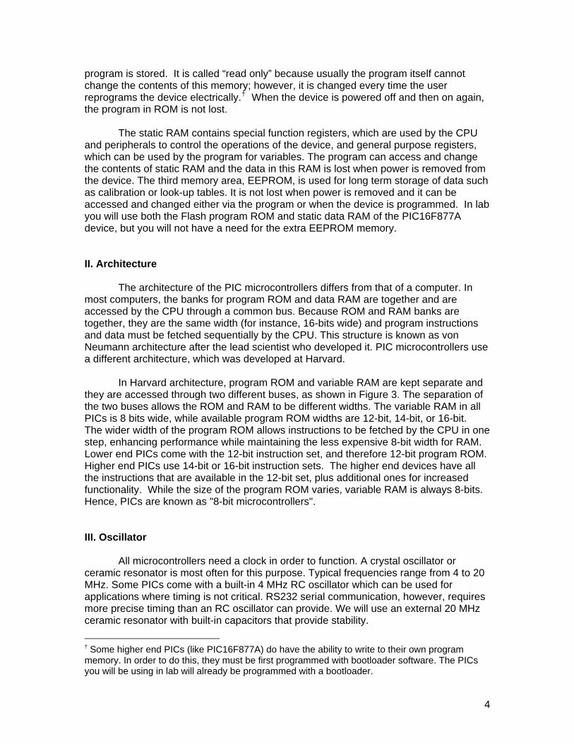
The architecture of the PIC microcontrollers differs from that of a computer. In most computers, the banks for program ROM and data RAM are together and are accessed by the CPU through a common bus. Because ROM and RAM banks are together, they are the same width (for instance, 16-bits wide) and program instructions and data must be fetched sequentially by the CPU. This structure is known as von Neumann architecture after the lead scientist who developed it. PIC microcontrollers use a different architecture, which was developed at Harvard.

In Harvard architecture, program ROM and variable RAM are kept separate and they are accessed through two different buses, as shown in Figure 3. The separation of the two buses allows the ROM and RAM to be different widths. The variable RAM in all PICs is 8 bits wide, while available program ROM widths are 12-bit, 14-bit, or 16-bit. The wider width of the program ROM allows instructions to be fetched by the CPU in one step, enhancing performance while maintaining the less expensive 8-bit width for RAM. Lower end PICs come with the 12-bit instruction set, and therefore 12-bit program ROM. Higher end PICs use 14-bit or 16-bit instruction sets. The higher end devices have all the instructions that are available in the 12-bit set, plus additional ones for increased functionality. While the size of the program ROM varies, variable RAM is always 8-bits. Hence, PICs are known as "8-bit microcontrollers".

III. Oscillator

All microcontrollers need a clock in order to function. A crystal oscillator or ceramic resonator is most often for this purpose. Typical frequencies range from 4 to 20 MHz. Some PICs come with a built-in 4 MHz RC oscillator which can be used for applications where timing is not critical. RS232 serial communication, however, requires more precise timing than an RC oscillator can provide. We will use an external 20 MHz ceramic resonator with built-in capacitors that provide stability.

† Some higher end PICs (like PIC16F877A) do have the ability to write to their own program memory. In order to do this, they must be first programmed with bootloader software. The PICs you will be using in lab will already be programmed with a bootloader.

4

program bus

FLASHprogram memory

CPU

Static RAM

Special Function Registers (controls operations)

General Purpose Registers (eg. variables)

EEPROM

long-term data storage (eg. calibration table)

14

8

data bus

8

program bus

FLASHprogram memory

CPU

Static RAM

Special Function Registers (controls operations)

General Purpose Registers (eg. variables)

EEPROM

long-term data storage (eg. calibration table)

14

8

data bus

8

Figure 3. Simplified schematic of architecture in a PIC16F877A device. The three regions of memory are shown. The Flash program memory is accessed via a 14-bit bus, while the static RAM and EEPROM are accessed via an 8-bit bus. IV. I/O ports The microcontroller communicates with the outside world via its I/O pins. When configured as an input, an I/O pin can read digitized information from a variety of sources, such as a sensor that measures some experimental variable, the status of a switch, or words typed into a keyboard. When used as outputs, the I/O pins can light an LED, sound an alarm, flip a switch, or send a message to an LCD or a computer screen. Most of the I/O pins are multiplexed with other functions, so that a pin can be used for either general purpose I/O or some other peripheral feature, such as programming.

The PIC16F877A device contains 33 I/O pins grouped into five I/O ports, PORTA

through PORTE. PORTA is 6 bits wide; that is, it has 6 pins. PORTE is three bits wide and the other ports (PORTB, PORTC, and PORTD) are all 8 bits wide. Pins from PORTA and PORTE together can be used as analog inputs for an on-board A/D converter. Some of the I/O pins in PORTB are used when programming and some pins in PORTC are used for serial communications.

Individually each I/O pin is capable of sinking (as in input) or sourcing (as an ouput) up to 25 mA. However, maximum combined currents for any one port should not

5

exceed 200 mA and maximum combined currents for all I/O ports should not exceed 250 mA. V. Registers

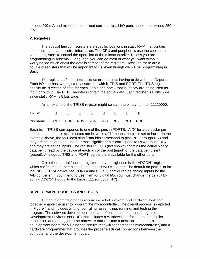
The special function registers are specific locations in static RAM that contain important status and control information. The CPU and peripherals use the contents in various registers to control the operation of the microcontroller. Unless you are programming in Assembly Language, you can do most of what you want without worrying too much about the details of most of the registers. However, there are a couple of registers that will be important to us, even though we will be programming in Basic.

The registers of most interest to us are the ones having to do with the I/O ports.

Each I/O port has two registers associated with it, TRIS and PORT. The TRIS registers specify the direction of data for each I/0 pin of a port – that is, if they are being used as input or output. The PORT registers contain the actual data. Each register is 8 bits wide, since static RAM is 8 bits wide.

As an example, the TRISB register might contain the binary number 11110000.

TRISB: _1_ _1_ _1_ _1_ _0_ _0_ _0_ _0_ Pin name: RB7 RB6 RB5 RB4 RB3 RB2 RB1 RB0

Each bit in TRISB corresponds to one of the pins in PORTB. A "0" for a particular pin means that the pin is set to output mode, while a "1" means the pin is set to input. In the example above, the four least significant bits correspond to pins RB0 through RB3 and they are set as outputs. The four most significant bits correspond to RB4 through RB7 and they are set as inputs. The register PORTB (not shown) contains the actual binary data being read by the device at each pin of the port (input) or the data being sent (output). Analogous TRIS and PORT registers are available for the other ports. One other special function register that you might use is the ADCON1 register which configures the port pins of the onboard A/D converter. The default on power up for the PIC16F877A device has PORTA and PORTE configured as analog inputs for the A/D converter. If you intend to use them for digital I/O, you must change the default by setting ADCON1 equal to the binary 111 (or decimal 7). DEVELOPMENT PROCESS AND TOOLS

The development process requires a set of software and hardware tools that together enable the user to program the microcontroller. The overall process is depicted in Figure 4 and includes writing, compiling, assembling, running, and testing the program. The software development tools are often bundled into one Integrated Development Environment (IDE) that includes a Windows interface, editor, compiler, assembler, and debugger. The hardware tools include a desktop computer, a development board for building the circuits that will connect to the microcontroller, and a hardware programmer that provides the proper electrical connections between the computer and the development board.

6

Write or editprogram in

PicBasic Pro

Compile andassembleprogram

Errors?

Done

Start

Load program onto microcontroller

Run anddebug

program

Errors?

yes

noyes no

Write or editprogram in

PicBasic Pro

Compile andassembleprogram

Errors?

Done

Start

Load program onto microcontroller

Run anddebug

program

Errors?

yes

noyes no

Figure 4. The development process.

Once the development process is complete, and both the circuit and program

have been thoroughly tested, the PIC can then run its application independently without being hooked up to the desktop computer. The application can even be hooked up to the web via an Ethernet connection for remote monitoring of the process. The set of development tools available in lab are discussed below. I. Software Programming Tools

Software packages for programming PICMicro® devices are available using

Assembly Language, C, or BASIC. Assembly Language is probably the best choice for learning about and really understanding the inner workings of a microcontroller, but the code is not the easiest to read and learn. Assembly language uses short mnemonics for program instructions and is specific to the CPU being programmed. Although most PICs have only about 35 instructions in their assembly code set, the language is quite powerful. However, it would take almost a whole semester course on microcontrollers to

7

learn enough to be able program the PIC in assembly language with the kind of control applications we are interested in as chemists. Higher level languages like C or Basic allow us to program a complex application in less time and with fewer lines of code. One line of C or Basic code can correspond to many lines of assembly code. Of course, one still needs to learn enough of the programming language to accomplish the task.

In lab we will use the PicBasic Pro™, a Basic compiler for PICs from microEngineering Labs, and MicroCode Studio Plus, an IDE from another vendor that provides a Windows interface, a program editor, an in-circuit debugger, and bootloading software. The PicBasic Pro™ compiler converts the user written BASIC code to assembly code. It then launches an assembler which converts the assembly code to a hex file. During the actual programming step – when the program is written to the PIC – the hex code is converted to binary machine code, which is the only code that the CPU can understand. Programming with PicBasic Pro™ will be discussed in more detail later. II. Development Board

You will use the 28/40 Development Board from Basic Micro. The board, shown in Figure 5, includes a socket for either a 28-pin or a 40-pin PIC, a connector for the power supply, a voltage regulator for the power supply, a status LED, a reset switch, and a connection for a hardware programmer. It also has a port and the proper circuitry for serial communications and a breadboard for building and testing circuits. The board is designed to allow programming of the PIC microcontroller while leaving the device and

breadboard

oscillator

microcontroller

reset switch

RJ-11jack

serialconnector

HIN232A

MC74HC4053Apower

status light

serial header

breadboard

oscillator

microcontroller

reset switch

RJ-11jack

serialconnector

HIN232A

MC74HC4053Apower

status light

serial header

Figure 5. The 28/40 Development Board

8

breadboard circuit in place. This feature is called in-system programming (ISP) or in-circuit programming (ICP). A socket for an external oscillator is available so the user can change the oscillator frequency. The data sheet and circuit diagram for the board are available on the Basic Micro website (www.basicmicro.com). Click on “Downloads”, then “PIC Prototyping Boards”, and finally “PIC 28/40 Prototype Board. III. Hardware Programmer

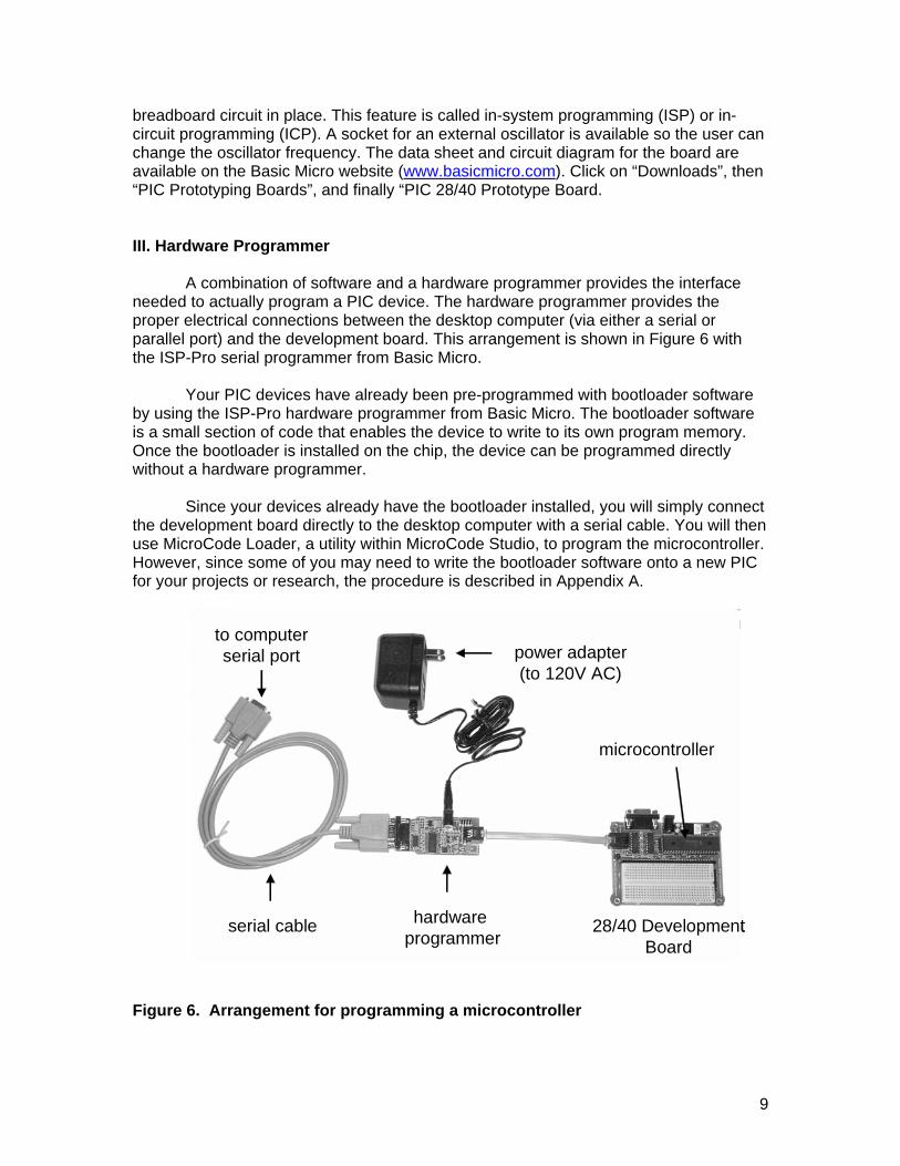
A combination of software and a hardware programmer provides the interface needed to actually program a PIC device. The hardware programmer provides the proper electrical connections between the desktop computer (via either a serial or parallel port) and the development board. This arrangement is shown in Figure 6 with the ISP-Pro serial programmer from Basic Micro.

Your PIC devices have already been pre-programmed with bootloader software

by using the ISP-Pro hardware programmer from Basic Micro. The bootloader software is a small section of code that enables the device to write to its own program memory. Once the bootloader is installed on the chip, the device can be programmed directly without a hardware programmer.

Since your devices already have the bootloader installed, you will simply connect

the development board directly to the desktop computer with a serial cable. You will then use MicroCode Loader, a utility within MicroCode Studio, to program the microcontroller. However, since some of you may need to write the bootloader software onto a new PIC for your projects or research, the procedure is described in Appendix A.

28/40 Development Board

hardware programmer

serial cable

power adapter (to 120V AC)

to computer serial port

microcontroller

28/40 Development Board

hardware programmer

serial cable

power adapter (to 120V AC)

to computer serial port

microcontroller

Figure 6. Arrangement for programming a microcontroller

9

PROGRAMMING WITH PICBASIC PRO™

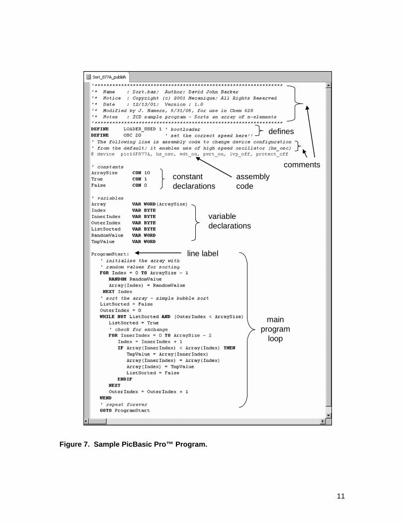
This introduction to PicBasic Pro™ is intended to help you get started with programming. It is not intended as a substitute for the help files and PicBasic manual. The PicBasic Pro manual is available on the microEngineering Labs web-site (http://www.melabs.com/resources/index.htm). Hard copies of the manual are also available in the lab. Of course, it is not expected that you will read the manual from cover to cover, but you will find it useful as a reference. You can ignore Chapter 3 on command line options. PicBasic Pro can be invoked from the DOS command line, but we will use it entirely from within MicroCode Studio. Help files for PicBasic are accessible from within MicroCode Studio on the lab computers. PicBasic Pro is a variation of the Basic Programming language. It has many of the same instructions you would find in other versions of Basic, such as GOTO, GOSUB, IF…THEN, and FOR…NEXT, to name a few. It also has many specialized instructions that are specific to PICmicro® devices. A sample program is shown in Figure 7. Some of the basics of using PicBasic are discussed below, followed by information related to I/O ports, serial communications, and mathematical calculations. I. Basics of PicBasic Pro Comments

Comments are preceded by an apostrophe ( ' ), a semi-colon (;), or the REM keyword. They are used to document the program. They are not read by the compiler and do not take up program space. You should include comments so that when you or someone else looks at your code, you can remember what you did and why. For example,

' Here is a comment line. Identifiers

Identifiers are names for variables, constants, or line labels. They are not case sensitive, must begin with a letter, and can contain letters, digits, and underscores. Examples are SetPoint, temp1, and go_figure. The identifiers "SetPoint", "setpoint", and "SETPOINT" are all equivalent. Variables

Variables are declared with the keyword VAR. Variables must be given a name (an identifier) and a size. Size options are BIT, BYTE, and WORD. For example, to declare a byte-sized variable called RandomValue, the code is: RandomValue VAR BYTE The words VAR and BYTE are shown in all bold capital letters above. You do not have to type them that way. You can type them in all lower case without bold. The editor in MicroCode Studio recognizes "var" and "byte" as reserved words and will format them in bold capitals. The formatting makes it easier to read the code and to find typographical errors. The compiler doesn't care about the case or formatting.

10

commentsassembly code

constant declarations

variable declarations

line label

main program

loop

defines

commentsassembly code

constant declarations

variable declarations

line label

main program

loop

defines

Figure 7. Sample PicBasic Pro™ Program.

11

Constants Constants are declared by the keyword CON. They can be defined in one of

three bases – decimal, binary, hexadecimal. They must be integers (more on this later). A binary number is preceded by a percent sign (%) and a hexadecimal number is preceded by a dollar sign ($). Range CON 50 ' Creates a constant called Range that equals 50. Mask CON %11110000 ' Sets Mask equal to the binary number 11110000. Temp1 CON $100 ' Creates constant Temp1 equal to hexadecimal

‘ $100, which equals 256 in the decimal base It is useful to give constants a name if you refer to the same number frequently in your program. Then, if you ever need to change that number, you only need to change it once – where you declared it – instead of searching through your code for every occurrence. Line Labels

Line labels are used to mark a line of code that you might want to reference in a GOSUB or GOTO statement. Line labels are identifiers followed by a colon. For instance, in Figure 7, "ProgramStart:" is a label for the main routine of the program that generates ten random numbers and sorts them. The last line of the program GOTO ProgramStart returns execution to the line labeled “ProgramStart:”, repeating the random number generation and sorting loop infinitely. DEFINE

DEFINE statements are used at the beginning of a program to change certain settings from their predefined values. For instance, you need a DEFINE statement to alert the compiler if you have a bootloader installed on your device. The correct statement for our purposes is: DEFINE LOADER_USED 1 ' Uses MicroCode Loader to program your device While most of what you type in the MicroCode editor is case insensitive, DEFINE statements are an exception. You should type DEFINEs in all capitals, as shown. You also need a DEFINE statement to declare the oscillator frequency. DEFINE OSC 20 ' Sets the oscillator frequency to 20 MHz All of your programs should have the two DEFINE statements above. Other DEFINE statements have to do with serial communication settings, timers, and parallel LCD displays. A complete list of them is in Appendix B of the PicBasic Pro manual.

12

II. I/O Ports and pins All of the registers of the PICmicro device can be accessed directly from PicBasic Pro. They can also be used in equations. Therefore, to set pins RB0 through RB3 to outputs and the remaining PORTB pins to input, use the command: TRISB = %11110000 Or, if you want to set the direction of just RB2 to output and leave the other pin directions unchanged, you can access pins individually by appending a decimal point and the pin number: TRISB.2 = 0

Once you have a pin set to output, you can use the PORTB keyword to set it high or low. For instance,

PORTB.2 = 1 ' Sets pin RB2 high PORTB.2 = 0 ' Sets pin RB2 low TRISC = %11111100 ' Sets pins RC0 and RC1 to output TRISC.0 = 1 ' Sets pin RC0 to one, or high You can also use the HIGH and LOW keywords to make a specific pin high or

low. When these commands are used, the pin is automatically made an output. HIGH PORTD.1 ' Makes pin RD1 an output and sets it high LOW PORTC.4 ' Makes pin RC4 an output and sets it low

Analogous commands can also be used for PORTA and PORTE. However, by default these ports are set to analog input for the onboard A/D converter. Before using them for digital I/O, you must change the register ADCON1 with the command ADCON1 = 7 ‘ Sets ports A and E to digital I/O; put this command ‘ near the beginning of the program Finally, if you will be referring to a particular I/O pin frequently, it may make your code more readable to assign the pin an alias. For instance, if you are using RB0 to light an LED, you can use the VAR keyword to create an alias, and then use the HIGH command to turn on the LED. LED VAR PORTB.0 ' Assigns the variable name "LED" to pin RB0 HIGH LED ' Turns on the LED III. Serial Communications in PicBasic Pro PicBasic Pro has several commands available for facilitating serial communications. We will use just three of them – HSERIN, HSEROUT, and SEROUT2.

13

The HSERIN and HSEROUT commands support asynchronous communications for PICmicro devices that have a hardware USART‡ interface. The PIC16F877A that you will use in lab has this type of interface. HSERIN is used for receiving data via pin 26 (RC7/RX) and HSEROUT is for transmitting data via pin 25 (RC6 /TX). The HSERIN and HSEROUT commands work only with these pins. The default format for the serial data is 8N1, which means that each character transmitted has 8 data bits, there is no parity bit, and 1 stop bit is used to signal the end of each character. The default baud rate is 2400. These default settings can all be changed via DEFINE statements. The syntax for the HSEROUT command is: HSEROUT [Item1, Item2, . . . ] The items can be numbers, variable names, or ASCII characters within quotation marks. The instruction interprets all numbers as their ASCII equivalent. For instance, if the variable SetPoint contains the number 75, the line HSEROUT ["The set point is: ", SetPoint] will generate on your terminal the message: The set point is: K The ASCII equivalent of the number 75 is the capital letter, K. This result is probably not what you would want. To display the actual number stored in SetPoint, use the keyword DEC before the variable name. For instance, HSEROUT ["The set point is: ", DEC SetPoint] will yield: The set point is: 75 Using the BIN keyword in place of DEC will cause the binary number 1001011 (the binary equivalent of 75) to be displayed, while using HEX displays the hexadecimal number 4B. We will use HSEROUT and HSERIN in the lab to send messages to and read messages from a computer terminal. We will use SEROUT2 to send messages to an LCD. Since SEROUT2 can be used on any I/O pin, the pin must be specified in the command. SEROUT2 also differs from HSEROUT in that the format for data transmission – called the mode – must be specified in the command line, as opposed to in a DEFINE statement. The syntax for SEROUT2 is: SEROUT2 pin, mode, [Item1, Item2, . . . ]

‡ USART stands for Universal Synchronous/Asynchronous Receiver/Transmitter. A USART is capable of sending and receiving data both synchronously (at fixed intervals with a separate line for a clock) or asynchronously (at random intervals with a specified format).

14

Mode is used to specify the baud rate and other parameters for serial communication. It is described more detail in the PicBasic Pro Compiler manual. Appendix A of the manual contains a table of mode values for common serial transmission parameters. For example, for a serial transfer using inverted TTL format at 2400 baud and no parity bit, the mode is 16780. To send the message "Hello, World!" to an LCD hooked up to portb.5, the following command would work: SEROUT2 portb.5, 16780, ["Hello, World!"] To display numbers, the keywords DEC, BIN, and HEX can be used just as with HSEROUT. For example: SEROUT2 portb.5, 16780, ["Set point: ", DEC 75] displays the message "Set point: 75" on the LCD. IV. Mathematical Calculations with PicBasic Pro Some care must be taken in performing mathematical calculations with PicBasic Pro. The data types (bits, bytes, and words) are all unsigned integers. The largest type, a word, is 16 bits and can range in value from 0 to 65,535 (216 – 1). If the result of a calculation is larger than 65,535, information is lost and the calculation yields an incorrect result. Similarly, if the result is a fraction, the number is truncated to an integer and is not rounded properly. All information to the right of the decimal place is lost. Floating point routines that address these problems are available for PicBasic Pro, but they are inconvenient to use and they take up a significant amount of memory. For the purposes of this course, a few simple strategies and tricks can be used to work around the problems. One strategy is to arrange the order of mathematical operations so that overflow (numbers too large) and fractions are avoided. Note that even if the final result is less than 65,535, the calculation will yield an incorrect result if any part of the calculation causes overflow. For instance, if X = 30,000, the statement Y = (X * 100) / 50 will not work because 30,000 * 100 = 3,000,000, which is greater than 65,535. Instead, the statement can be written Y = X * (100/50), because the quantity in parentheses is evaluated first. Alternatively, one can simplify the equation to: Y = X * 2. Notice that none of the above equations will work if X is greater than 32,767.

15

Another strategy for numbers that are too large is to shift the binary equivalent of the number to the right by n bits by dividing by 2n. For instance if X = 40,000, dividing by 22 will shift the binary value of X to the right by 2 bits, making it 10,000. Subsequent multiplications can then be performed with less risk of overflow. Of course, you will lose some information because you have dropped the two least significant bits of the number. If the number is very large, the loss of these last two bits will be insignificant. Also, you must keep track of the fact that your number has been shifted and take care to also shift any numbers that you will add to or subtract from X.

To handle fractions or decimal numbers, you can shift the binary equivalent (or

the base 10 number) to the left n places by multiplying by 2n (or by 10n). For instance, if you want to keep track of a temperature to a tenth of a degree, you can deal with the number in terms of tenths of a degree, effectively multiplying the temperature by 10. That is, 25.2 degrees becomes 252 tenths of a degree.

You will see more examples of these strategies as you work through the

Microcontroller Lab. In general, it is a good idea to test your program calculations with a hand-held calculator to ensure that you avoid problems with overflow and fractions. MICROCONTROLLER LAB UNIT

This document provides some of the background information needed for the three-part unit on Microcontrollers and Feedback. The three parts are:

PART A: Programming the Microcontroller PART B: Monitoring an Experiment PART C: Feedback Control of an Experiment

By the end of the three weeks you will have learned how to use a microcontroller to control the temperature of a heater block. In the course of your research, you will probably encounter other problems that are also well-suited to feedback control with a microcontroller. It is hoped that you will be able to build on what you learn in this unit to solve such problems in your research.

16

APPENDIX A: Installing a Bootloader on PIC Device

Some of the higher-end PIC devices, like PIC16F877A, have the ability to write to their own program memory. In order to use this feature, you must first program the bootloader software onto the PIC. Mecanique provides bootloader software that, once installed on your PIC, can then be used to program your application onto the PIC from MicroCode Studio Plus. The bootloader software is unique for each PIC device and oscillator used. The steps for programming the PIC with the bootloader are given below. The physical arrangement is shown in Figure 6. 1. Attach the serial cable from your computer to the ISP-Pro programming board. 2. Attach the ISP-Pro board to the 2840 Development Board using the RJ11 telephone-style cable. You should already have your PIC device and oscillator installed on the board. 3. Plug in the power adapter into the ISP-Pro Board. This connection will also provide power to the development board. (A second power adapter is not needed.) 4. Run Basic Micro ISP-Pro IDE from the start menu on the computer. 5. Open the appropriate hex file that contains the bootloader software. The files are located in the directory "C:\Program Files\Mecanique\MCSP\MCLoader". For instance the PIC16F877A device with a 20 MHz oscillator uses the file "16F877A_20.HEX". Choose the appropriate device family and processor name when prompted and then click "OK". 6. Click "Program" from the Tools menu or from the toolbar. If you get an "unable to verify" message, try reprogramming. 7. Exit Basic Micro ISP-Pro IDE. Disconnect the power supply, the serial cable, and the RJ11 cable. 8. Your chip now has the bootloader software installed on it. You can now hook the 2840 Development Board directly to your computer via the serial cable. Then you can run Microcode Loader within the Microcode Studio Plus IDE to program your device with your application program. You no longer need the ISP-Pro hardware programmer. ** This Laboratory was developed by Jeanne Hamers in September of 2005.

17

Chemistry 628 University of Wisconsin-Madison Unit 3 Lab: Microcontrollers and Feedback

PART A: PROGRAMMING THE MICROCONTROLLER

This lab is the first of a series of three on Microcontrollers and Feedback. In this part you will learn how to program a PICmicro® brand microcontroller to perform various functions. You will use the compiler PicBasic Pro™ within Microcode Studio Plus IDE (integrated development environment) to program, test, and debug applications involving I/O and serial communications. In later labs you will interface the microcontroller to a temperature sensor and use it to control the temperature of an aluminum block. Before beginning this lab you should have already read the Laboratory Unit on Microcontrollers and Feedback: An Introduction and completed Question 3 of the Report for Part A. EQUIPMENT Microcode Studio Plus IDE and PicBasic Pro™ compiler (installed on desktop computer) Basic Micro 28/40 Dev Board PIC16F877A microcontroller (with bootloader installed) AC Power Adaptor (9 V, 500 mA) Serial Cable 20 MHz oscillator with built in capacitors BPI-216 Serial LCD Module Resistors (three 470 Ω and one 10 kΩ) 2 LEDs (two different colors) Pushbutton switch BACKGROUND Every circuit you build with the microcontroller must have the connections shown in Figure 1. Most of the connections shown are already done for you on the 28/40 Development Board because they are connections that you always need. For instance, the +5 V power supply (Vdd) to pins 11 and 32 and the ground (Vss) connections to pins 12 and 31 are already wired on the printed circuit board. Further connections to +5 V and ground, in addition to any connections to I/O pins, can be made on the headers next to the breadboard. Pins 13 and 14 of the PIC are wired to the oscillator socket next to the PIC. MCLR and the Bootloader

The MCLR circuitry shown in the figure is also already wired on the development board. MCLR stands for "master clear." It is attached to the +5 V power supply through diode D1 and a 10 kΩ pull-up resistor. During normal operation, when the PIC is running a program, MCLR is held high. When this pin is toggled low and then high (by pushing and releasing the switch S1), the device is reset and the program that is stored on the PIC starts over at the beginning. MCLR is also used to enable programming of

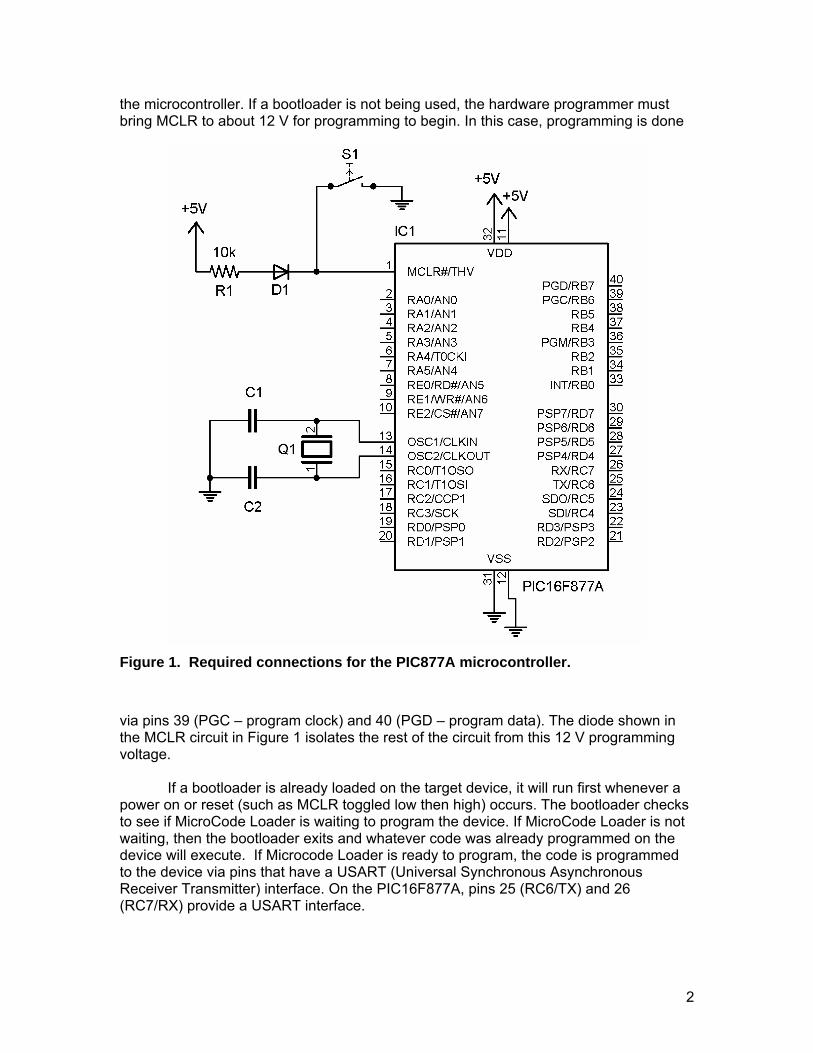
the microcontroller. If a bootloader is not being used, the hardware programmer must bring MCLR to about 12 V for programming to begin. In this case, programming is done

Figure 1. Required connections for the PIC877A microcontroller. via pins 39 (PGC – program clock) and 40 (PGD – program data). The diode shown in the MCLR circuit in Figure 1 isolates the rest of the circuit from this 12 V programming voltage.

If a bootloader is already loaded on the target device, it will run first whenever a power on or reset (such as MCLR toggled low then high) occurs. The bootloader checks to see if MicroCode Loader is waiting to program the device. If MicroCode Loader is not waiting, then the bootloader exits and whatever code was already programmed on the device will execute. If Microcode Loader is ready to program, the code is programmed to the device via pins that have a USART (Universal Synchronous Asynchronous Receiver Transmitter) interface. On the PIC16F877A, pins 25 (RC6/TX) and 26 (RC7/RX) provide a USART interface.

2

Serial Communication

The PIC device can send and receive serial data via any of its I/O pins, including the USART. However the PIC and the device it is communicating with – such as a computer, an instrument, or an LCD display – must agree on the format of the data. RS-232 and inverted TTL are two standards that are commonly used. Programming via Microcode Loader requires RS-232 format, while displaying a message on an LCD can be done with either format. Both communication standards have certain requirements for the voltage levels of the signals. For RS-232, a hardware interface between the PIC and the computer– called a serial line driver – is required to ensure that the voltage levels are appropriate.

The 28/40 Development Board contains an RS-232 line driver. The 4-pin serial

header next to the microcontroller socket provides access to this driver. Because different users might want to use different I/O pins for RS-232 serial communication tasks, this header is NOT already wired to the microcontroller socket. The user must jumper the header connections to the appropriate pins of the PIC device using the I/O header next to the breadboard. Therefore, when programming the microcontroller with the bootloader via the USART, TX and RX on the driver header must be wired to the USART pins 25 (RC6/TX) and 26 (RC7/RX) pins of the PIC. EXPERIMENTAL PROCEDURE A. EXPLORING MICROCODE STUDIO In this exercise, you are introduced to the MicroCode Studio IDE, including the editor, the loader, the debugger, and help files. Getting Started 1. Launch MicroCode Studio from the Start Menu. The window is shown in Figure 2. The interface consists of a set of dropdown menus, toolbars, a code explorer window, and a main editing window. 2. Explore the various dropdown menus. The File and Edit menus have the typical options you see in most Windows programs. Shortcuts to many of these options are located on the editor toolbar. Hoover the cursor over the toolbar icons to see what they do. 3. The large, main window is for editing the PicBasic source code. Load the program "Sort_877A.pbp" by clicking "File/Open" and navigating to the folder "C:\Chem628_PIC\PicIntro". This is a program that sorts an array of randomly generated numbers. Notice the formatting of the file. As you type a program, the editor automatically formats the text. The formatting details can be changed by the user, but we will assume here that the default settings are in place. 4. Comment lines begin with an apostrophe ( ' ), semi-colon ( ; ) or the keyword REM. The editor automatically changes any line that begins with these symbols to blue italics. Comment lines are ignored when the compiler is run and they are not written to the

3

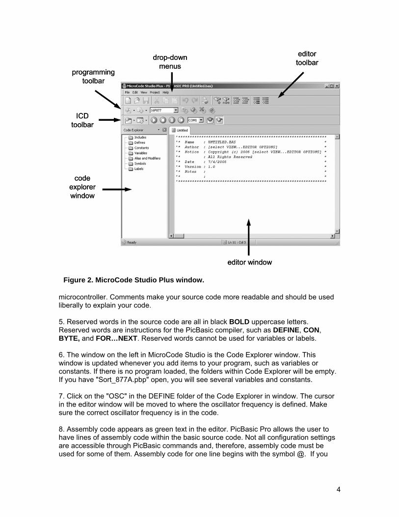
editor window

code explorer window

drop-down menus

ICD toolbar

editor toolbar

programming toolbar

editor window

code explorer window

drop-down menus

ICD toolbar

editor toolbar

programming toolbar

microcontroller. Comments make your source code more readable and should be used liberally to explain your code.

Figure 2. MicroCode Studio Plus window.

5. Reserved words in the source code are all in black BOLD uppercase letters. Reserved words are instructions for the PicBasic compiler, such as DEFINE, CON, BYTE, and FOR…NEXT. Reserved words cannot be used for variables or labels. 6. The window on the left in MicroCode Studio is the Code Explorer window. This window is updated whenever you add items to your program, such as variables or constants. If there is no program loaded, the folders within Code Explorer will be empty. If you have "Sort_877A.pbp" open, you will see several variables and constants. 7. Click on the "OSC" in the DEFINE folder of the Code Explorer in window. The cursor in the editor window will be moved to where the oscillator frequency is defined. Make sure the correct oscillator frequency is in the code. 8. Assembly code appears as green text in the editor. PicBasic Pro allows the user to have lines of assembly code within the basic source code. Not all configuration settings are accessible through PicBasic commands and, therefore, assembly code must be used for some of them. Assembly code for one line begins with the symbol @. If you

4

have more than one line of assembly code, you can sandwich them between the instructions ASM and ENDASM.

The program "Sort_877A.pbp" has one line of assembly code to change the default configuration. PicBasic Pro assumes a default oscillator of 4 MHz, which uses "xt_osc" in the configuration specification. Since we are using a 20 MHz oscillator, we need to use "hs_osc".

9. Investigate the help topics available in Microcode Studio (Help/Help Files). Most parts of the PicBasic Pro manual are included in these help files. In addition, help files are available for MicroCode Studio, the editor, and MicroCode Loader. Locate the help file for PicBasic commands. You can use this help file to find the proper use and syntax for any PicBasic instruction. 10. Look over the code in the program "Sort_877A". You will see that constants and variables are declared near the beginning of the program, after the DEFINEs and device configuration. The first FOR…NEXT loop fills an array with random numbers and the second FOR…NEXT loop sorts those numbers. The program repeats itself until stopped by the user. Next you will write (or “burn”) this program to the microcontroller. . Programming the PIC 1. Plug an oscillator into the socket of the 28/40 Development Board. 2. Since you will use the bootloader for programming, jumper RX and TX to the appropriate pins of the PIC device. 3. Connect the development board to the desktop computer via the serial cable. NOTE: Apply power in the next step only after all other connections have been made and you and your partner have double-checked your circuit. Building circuits on the breadboard and connecting wires while power is already applied could cause damage to the microcontroller or other components. The development board should have an on/off switch, but it does not. 4. Apply power to the board with the power supply cable. 5. Choose the correct device from the drop down menu on the toolbar. 6. Program the device by clicking on the "compile and program" button. You will be prompted for a filename. Navigate to your own folder within C:\Chem628_Pic and rename your source code to save your version of the program. 7. If you have received no error messages, you have probably successfully programmed the PIC. However, you really can't tell – the program doesn't have any I/O instructions that provide information to the user. It may or may not be happily sorting random numbers! Usually your programs will include instructions that let you know what the program is doing, such as sending a message to an LCD or flashing a light. You can also monitor what your program is doing by using the in-circuit debugger (ICD).

5

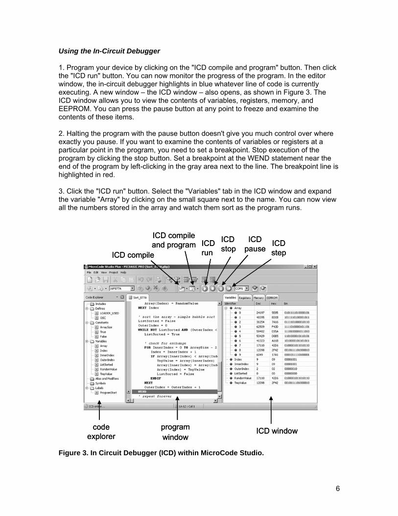
Using the In-Circuit Debugger 1. Program your device by clicking on the "ICD compile and program" button. Then click the "ICD run" button. You can now monitor the progress of the program. In the editor window, the in-circuit debugger highlights in blue whatever line of code is currently executing. A new window – the ICD window – also opens, as shown in Figure 3. The ICD window allows you to view the contents of variables, registers, memory, and EEPROM. You can press the pause button at any point to freeze and examine the contents of these items. 2. Halting the program with the pause button doesn't give you much control over where exactly you pause. If you want to examine the contents of variables or registers at a particular point in the program, you need to set a breakpoint. Stop execution of the program by clicking the stop button. Set a breakpoint at the WEND statement near the end of the program by left-clicking in the gray area next to the line. The breakpoint line is highlighted in red. 3. Click the "ICD run" button. Select the "Variables" tab in the ICD window and expand the variable "Array" by clicking on the small square next to the name. You can now view all the numbers stored in the array and watch them sort as the program runs.

programwindow

ICD window

ICD run

ICDstop

ICD pause

ICD step

code explorer

ICD compile

ICD compile and program

programwindow

ICD window

ICD run

ICDstop

ICD pause

ICD step

code explorer

ICD compile

ICD compile and program

Figure 3. In Circuit Debugger (ICD) within MicroCode Studio.

6

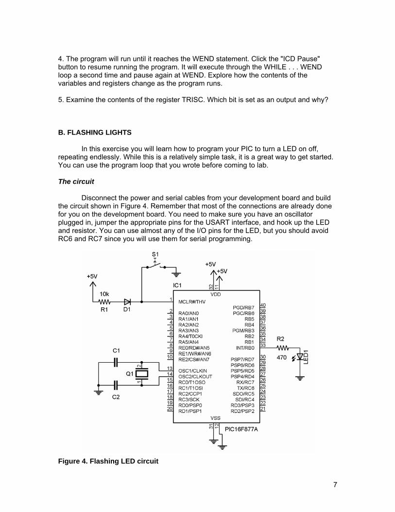
4. The program will run until it reaches the WEND statement. Click the "ICD Pause" button to resume running the program. It will execute through the WHILE . . . WEND loop a second time and pause again at WEND. Explore how the contents of the variables and registers change as the program runs. 5. Examine the contents of the register TRISC. Which bit is set as an output and why? B. FLASHING LIGHTS In this exercise you will learn how to program your PIC to turn a LED on off, repeating endlessly. While this is a relatively simple task, it is a great way to get started. You can use the program loop that you wrote before coming to lab. The circuit

Disconnect the power and serial cables from your development board and build the circuit shown in Figure 4. Remember that most of the connections are already done for you on the development board. You need to make sure you have an oscillator plugged in, jumper the appropriate pins for the USART interface, and hook up the LED and resistor. You can use almost any of the I/O pins for the LED, but you should avoid RC6 and RC7 since you will use them for serial programming.

Figure 4. Flashing LED circuit

7

The program 1. Click File/New in MicroCode Studio. Edit the header to include an appropriate filename, your name, and your section. You should use the default ".pbp" file extension. Save this file in your directory. 2. Write a program to turn the LED on for one second and then off for one second, repeating infinitely. Remember to use the proper DEFINE statements for the bootloader and the oscillator frequency. Also include the proper configuration statement in assembly code for the high speed oscillator. Other commands that you might find useful are TRISB, PORTB, HIGH, LOW, PAUSE, and GOTO. 3. Check your program for syntax errors by clicking the compile button. You don't need to be connected to the circuit to compile the program. 4. If you haven't done so already, you can now connect first the serial cable and then the power cable to your development board. REMINDER: Apply power only after all other connections have been made and you and your partner have double-checked your circuit. 6. Click compile and program to test your application. Make any necessary revisions to your program or circuit until it works. Are the on and off times of the LED accurate? Experiment with a couple of different on and off times. 7. Use a FOR…NEXT loop to change your program so that it turns the LED on off ten times, instead of repeating infinitely. Since this program is not an infinite loop, you should use the keyword "END" at the end of your program. The “END” instruction stops program execution and puts the device in a low power mode.

Compile and test your new program until it works. Demonstrate your program for the instructor.

8. Disconnect the serial cable from the development board and press the reset switch. Does the program still run as expected? Once the microcontroller is programmed, it should be able to operate independently of the desktop computer.

C. PUSHBUTTON CONTROL In this exercise you will use the microcontroller to read the state of a pushbutton switch. Pins 1 and 4 of the pushbutton are connected together and pins 2 and 3 are connected. The switch is normally open, which means it is open when the button is not pressed. The circuit 1. Disconnect the power and serial cables from the development board.

8

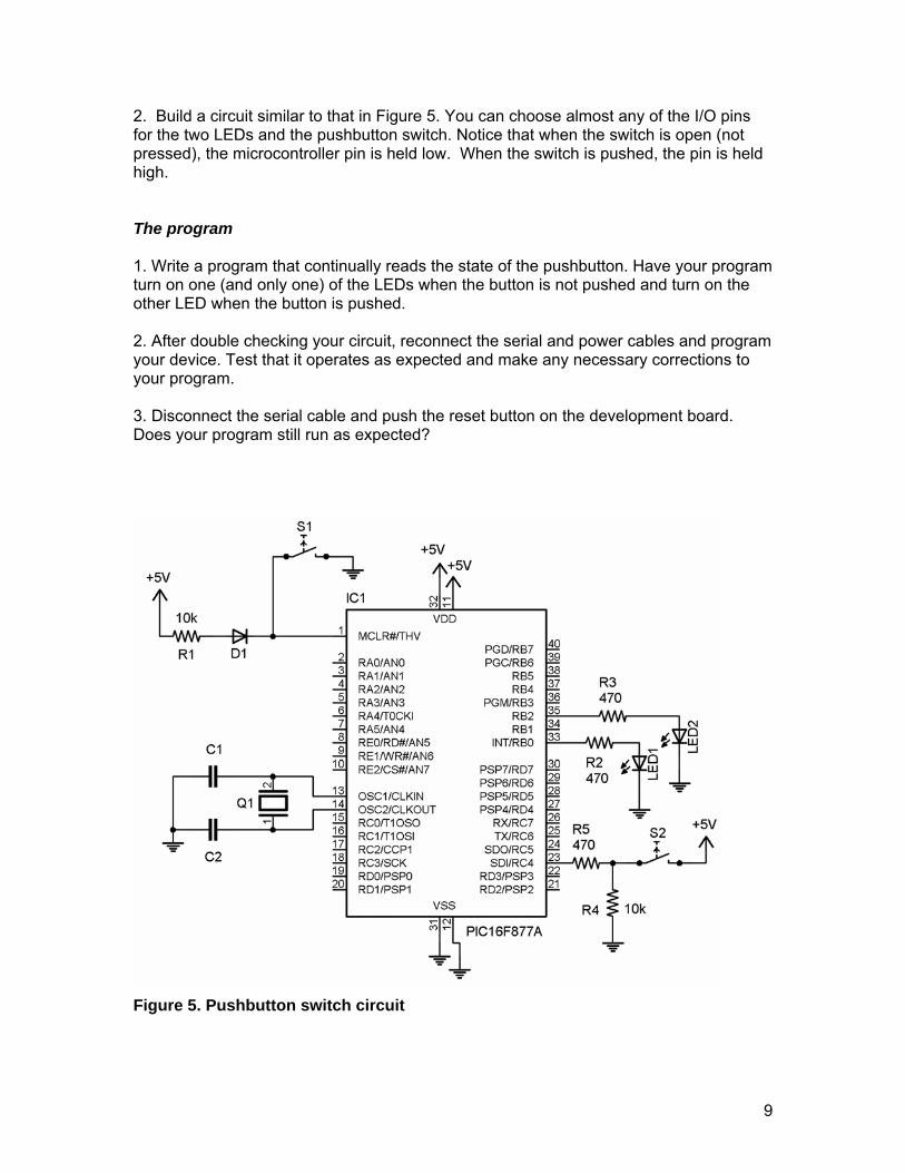
2. Build a circuit similar to that in Figure 5. You can choose almost any of the I/O pins for the two LEDs and the pushbutton switch. Notice that when the switch is open (not pressed), the microcontroller pin is held low. When the switch is pushed, the pin is held high. The program 1. Write a program that continually reads the state of the pushbutton. Have your program turn on one (and only one) of the LEDs when the button is not pushed and turn on the other LED when the button is pushed. 2. After double checking your circuit, reconnect the serial and power cables and program your device. Test that it operates as expected and make any necessary corrections to your program. 3. Disconnect the serial cable and push the reset button on the development board. Does your program still run as expected?

Figure 5. Pushbutton switch circuit

9

D. SERIAL COMMUNICATION WITH AN LCD In this exercise you will program the PIC to send a message to a liquid crystal display (LCD). The PIC can communicate with an LCD via either a parallel or serial interface. Using a parallel interface requires that either 4 or 8 I/O pins be dedicated to the display, while a serial interface requires only one pin. We will use the BPI-216 Serial LCD module from Scott Edwards Electronics.

The LCD module includes a small printed circuit board attached to the back of the LCD. This board provides the interface that allows the LCD to receive data either in RS-232 or inverted TTL format and at 2400 or 9600 baud. The user can send either text (such as a message) or instructions (such as clear the screen or move the cursor) on the LCD. The default mode is text. Each instruction must be preceded by an instruction prefix, which is the ASCII character 254. We will use the SEROUT2 command to send data to the LCD in inverted TTL format. The format for the command is:

SEROUT2 pin, mode, ["type your message here"] Substitute the appropriate pin name for "pin" and the mode number for "mode". For inverted TTL at 2400 baud, the mode number is 16780, and at 9600 baud the mode is 16468. (See Appendix A of the PicBasic Pro Compiler manual for a table of mode values for use with SEROUT2.) Often before sending a message, you will want to clear the screen. The format for that instruction is: SEROUT2 pin, mode, [254, 1] ' Clears LCD screen In the above command, the number "254" alerts the LCD that an instruction follows and number "1" is the instruction code for clearing the screen. See page 4 of the LCD manual for the other instruction codes.* Finally, the LCD needs about one second to come up to power when first turned on. This delay means that for short programs, you might need a PAUSE command before sending a message to the display. The circuit 1. Examine the LCD module and locate the printed circuit board attached to the back of it. Notice the chip on the board – it is a PICmicro® device that has been factory programmed to control the serial interface! Near the chip are two switches. If you hold the module so that the writing is right-side up, the switch on the left provides a choice for a baud rate of 2400 or 9600. The right hand switch is for a backlight on the LCD. 2. Decide which baud rate you want to use and set the switch to your choice.

* You can find the short (8 pages) LCD manual at online at http://www.seetron.com/slcds.htm. Copies will also be available in lab.

10

3. If your module has a backlight, ensure that it is off (switch down). The backlight draws too much current. 4. Disconnect the power supply from the development board. 5. Attach the LCD cable to the LCD module. The cable has a 5 pin header in a palindrome arrangement. It doesn't matter which orientation you plug it in, as long as all 5 pins are in the socket. 6. Connect +5 (red wire) and ground connections (black wire) of the LCD to Vdd and Vss respectively on the development board. Double-check these connections. Accidentally reversing +5 and ground will damage the LCD module. 7. Connect the serial line to an I/O pin of your choice. The program 1. Open a new file within Microcode Studio, edit the header, and save the new file in your directory. 2. Write a short program that sends a message to the LCD. Remember to use the appropriate DEFINEs and configuration statements. 3. Compile your program and correct any syntax errors. 4. Apply power to the development board and program the PIC. Make any necessary changes so that your message displays as expected. 5. Send a two-line message to the LCD. You will need to move the cursor to the proper position on the screen for the second line. Demonstrate your working program to the instructor. E. SERIAL COMMUNICATION WITH A TERMINAL Sending messages to an LCD is a great way to monitor your application, especially once your program is tested and being used remotely without a desktop computer. However, during the course of program development, it is convenient to establish serial communications with a terminal display. MicroCode Studio has a built in terminal display window that we can use to both send and receive messages.

Almost any I/O port can be used for serial communications if it isn't already tied up with some other function. For communications with a terminal, the pins RC6 and RC7 will be the most convenient for us because they are the USART pins. These are the same pins that we use when programming the microcontroller with the bootloader. When programming, we have the RX and TX ports on the development board jumpered to RC6 and RC7. If you choose to use different I/O pins for terminal communications, you need to move these jumpers to the appropriate pins each time after programming and move them back to RC6 and RC7 each time before programming. Obviously, it is more convenient not to have to keep switching the jumpers.

11

The circuit Use the circuit shown in Figure 4 from Part B of this lab. The program The program for testing serial communications via a terminal has been written for you and is shown in Figure 6. In this program, HSERIN and HSEROUT are used and two new DEFINE statements appear. Both DEFINEs are related to serial communications with the USART interface on the PIC. The first DEFINE sets the baud rate and is only necessary if you are using a different baud rate than the default 2400. The second DEFINE clears the USART buffer if it overflows. After the DEFINE statements, a variable array called “Message” is declared. This array of ten byte-sized variables will hold a message typed by the user.

The program contains a main loop and a timeout loop. In the first loop, the program turns on the LED at portb.0 and uses HSEROUT to prompt the user to input a word. HSERIN reads the word typed by the user. If no word is entered after 30 seconds (30,000 msec), the program jumps to the loop labeled “timeout”. (See the PicBasic Pro manual for more details on the syntax for HSERIN.) The timeout loop flashes the LED to indicate a timeout error has occurred. If a word is entered before the timeout, it is echoed by another HSEROUT instruction. The number “13” in the HSEROUT commands is the ASCII control character for a carriage return.

1. Open the file "Serial_IO_string.pbp" in the C:\Chem628_Pic\PicIntro directory. Change the DEFINE statement to the baud rate of your choice. Program your device with "Serial_IO_string.pbp". 2. Open the Serial Communicator window in MicroCode Studio (View/Serial Communicator). 3. Check the settings in the left-hand panel. You should be using COM1, your choice of baud rate, no parity bit, byte size of 8, and one stop bit. Make any necessary changes. 4. Check the settings on the transmit window by clicking on the down arrow located on the right-hand side of the header bar of the transmit window. Select "Auto Clear After Transmit" and deselect "Transmit on Carriage Return". 5. Click the connect icon in the toolbar to establish a connection between the communicator to the development board. 6. Reset the development board. The prompt message should appear in the receive window. 7. Test the program by typing various words in the transmit window. End every word with a space and then click SEND. If you wish to clear either window, use the clear option on the right-hand down arrows. If the program enters the timeout loop, reset the development board to continue. Experiment with different baud rates. Since both the serial communicator and the bootloader use COM1, you will need to disconnect the serial communicator when you reprogram.

12

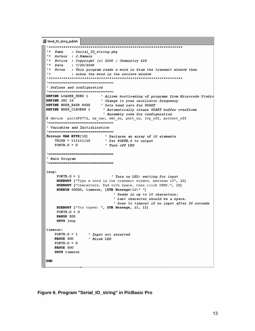
Figure 6. Program "Serial_IO_string" in PicBasic Pro

13

8. Now click “Save As” and save the program with a different name in your own directory. Modify the program to allow inputting a sentence up to 50 characters long. Change the termination character to something else, so that you can use spaces in your sentence. F. PUTTING IT ALL TOGETHER For the final section of this lab, write a program that combines several of the tasks that you have learned about. Your program should first prompt the user with a menu of choices. The choices should include 1) blinking an LED, 2) reading the status of a pushbutton switch and report it’s state on the terminal, 3) sending a message to the LCD, and 4) do all of the above. The microcontroller should perform the user chosen task and then prompt the user again with the same choices. Demonstrate your working program to the lab instructor. REPORT

For your report, turn in the answers to the questions in “Report for Part A” at the

beginning of your next lab period.

14

Chemistry 628 University of Wisconsin-Madison Unit 3 Lab: Microcontrollers and Feedback

PART B: MONITORING AN EXPERIMENT This lab is the second of three in the Microcontroller and Feedback Unit. In this part you will use the microcontroller to monitor temperature as measured with a chromel-alumel (Type K) thermocouple. Because thermocouple voltages are relatively small, an AD595 thermocouple amplifier will be used to boost the signal before sending it to an ADC (analog-to-digital converter). The microcontroller will then be programmed to read the output of the ADC and report the result to the user via an LCD or the computer terminal. You will also use a plotting utility, Stamp Plot Lite, to graph data as it is acquired. EQUIPMENT From Part A lab: Microcode Studio Plus IDE and PicBasic Pro™ compiler (installed on desktop computer) Basic Micro 28/40 Dev Board PIC16F877A microcontroller (with bootloader installed) AC Power Adaptor (9 V, 500 mA) Serial Cable 20 MHz oscillator with built in capacitors BPI-216 Serial LCD Module New for Part B: AD595AQ thermocouple amplifier LT1286 ADC LM285 1.2 V reference Capacitors (10 μF tantalum, 0.1 μF) Resistors (two 10 kΩ) Chromel-alumel (Type K) thermocouple wire with two junctions Chromel-alumel (Type K) thermocouple wire with one junction Thermometer Styrofoam cup with ice BACKGROUND

A thermocouple is a junction of two dissimilar metals that can be used to measure temperature. When two dissimilar metals are in contact, a small but measurable potential occurs across the junction. The magnitude of the potential (the voltage) depends on both the temperature and the composition of the two metals. The thermocouple that you will use consists of a junction between chromel (an alloy of nickel and chromium) and alumel (an alloy of nickel and aluminum).

One can see the effect of temperature on a thermocouple junction simply by measuring the voltage across the junction, as shown in Figure 1. Note that in this

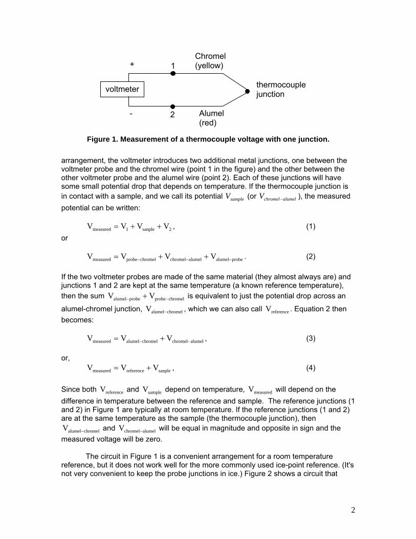
Chromel (yellow)

Alumel (red)

+

-

voltmeter thermocouple junction

1

2

Figure 1. Measurement of a thermocouple voltage with one junction. arrangement, the voltmeter introduces two additional metal junctions, one between the voltmeter probe and the chromel wire (point 1 in the figure) and the other between the other voltmeter probe and the alumel wire (point 2). Each of these junctions will have some small potential drop that depends on temperature. If the thermocouple junction is in contact with a sample, and we call its potential (or ), the measured potential can be written:

sampleV alumelchromelV −

2sanple1measured VVVV ++= , (1)

or

probealumelalumelchromelchromelprobemeasured VVVV −−− ++= . (2)

If the two voltmeter probes are made of the same material (they almost always are) and junctions 1 and 2 are kept at the same temperature (a known reference temperature), then the sum is equivalent to just the potential drop across an

alumel-chromel junction, , which we can also call . Equation 2 then becomes:

chromelprobeprobealumel VV −− +

chromelalumelV − referenceV

alumelchromelchromelalumelmeasured VVV −− += , (3)

or,

sanplereferencemeasured VVV += , (4) Since both and depend on temperature, will depend on the difference in temperature between the reference and sample. The reference junctions (1 and 2) in Figure 1 are typically at room temperature. If the reference junctions (1 and 2) are at the same temperature as the sample (the thermocouple junction), then

and will be equal in magnitude and opposite in sign and the measured voltage will be zero.

referenceV sampleV measuredV

chromelalumelV − alumelchromelV −

The circuit in Figure 1 is a convenient arrangement for a room temperature

reference, but it does not work well for the more commonly used ice-point reference. (It's not very convenient to keep the probe junctions in ice.) Figure 2 shows a circuit that

2

uses a second thermocouple junction that can easily be placed in ice for the reference. There are still two junctions between the voltmeter probes and the thermocouple, but

voltmeter

Chromel (yellow)

Alumel (red)

Alumel (red)

reference junction

sample junction 12

Figure 2. Measurement of thermocouple voltage two junctions.

both junctions are between alumel and a voltmeter probe. One potential drop goes from the positive probe to alumel while the second drop goes from alumel to the probe. If these junctions are at the same temperature, their potentials will be equal in magnitude but opposite in sign, and they will cancel. The resulting measured voltage will again be the sum of the sample and reference potentials (as in Equation 4), where now is the voltage at the second thermocouple junction, not the sum of the potentials at the probe junctions.

referenceV

To get the temperature from the measured voltage, one consults a standard reference table1. This table is for a Type K thermocouple, which is just another name for the chromel-alumel thermocouple you will use in this lab. The voltages in the reference tables are usually with respect to a reference junction in ice at 0°C. That is, the voltage listed is the difference between the voltage of the sample junction and the voltage of an ice reference junction.

1 Appendix A. The table can also be found online at the Omega Engineering Technical Reference website (http://www.omega.com/thermocouples.html). This web page contains numerous links to thermocouple resources including product information, technical information, and many reference tables. The link "Using Thermocouples" (or http://www.omega.com/temperature/Z/pdf/z021-032.pdf) is particularly instructive. The direct link to the reference table is http://www.omega.com/temperature/Z/pdf/z204-206.pdf)

3

EXPERIMENTAL PROCEDURE A. AMPLIFYING THE THERMOCOUPLE SIGNAL

In the temperature range from 0 to 100°C, the chromel-alumel thermocouple voltage changes only about 40 to 41 μvolts per °C. Therefore, accurately measuring a 1°C temperature change using a DMM is quite difficult. One could use a basic op amp to amplify the signal. It is even more convenient to use an amplifier specially designed for thermocouples, such as the AD595. In this exercise, you will investigate the thermocouple signal both before and after amplification. Thermocouple signal before amplification For this part, use the thermocouple wire that has two junctions. Place one junction (the reference) in ice and use the other junction for measurement.

Using both a thermometer and the thermocouple (as shown in Figure 2), measure the temperature of the following:

a) ice b) room temperature c) yourself - by warming the temperature probe between your two fingers.

Using the thermocouple table, what temperatures do your measurements

correspond to? Does your thermocouple measurement agree with the thermometer measurement?

Thermocouple signal after amplification The AD595 amplifier has built-in compensation for an ice point reference. That is, in addition to amplifying the thermocouple voltage (the gain is 247.3), it automatically measures the surrounding reference temperature and adds an appropriate voltage to the output. The net result is that the amplifier outputs a voltage of 0 mV at 0 °C. The odd value for the gain (247.3) was chosen so that the output voltage changes 10 mV for every °C change in temperature. This voltage change of 10 mV per °C is much more easily measured than the unamplified 40 μV per °C.

Using the thermocouple wire with only one junction, wire the TC amplifier as shown in Figure 3 on the breadboard of the 28/40 Development Board. Use Vdd and Vss from the development board for +5 V and ground respectively.

4

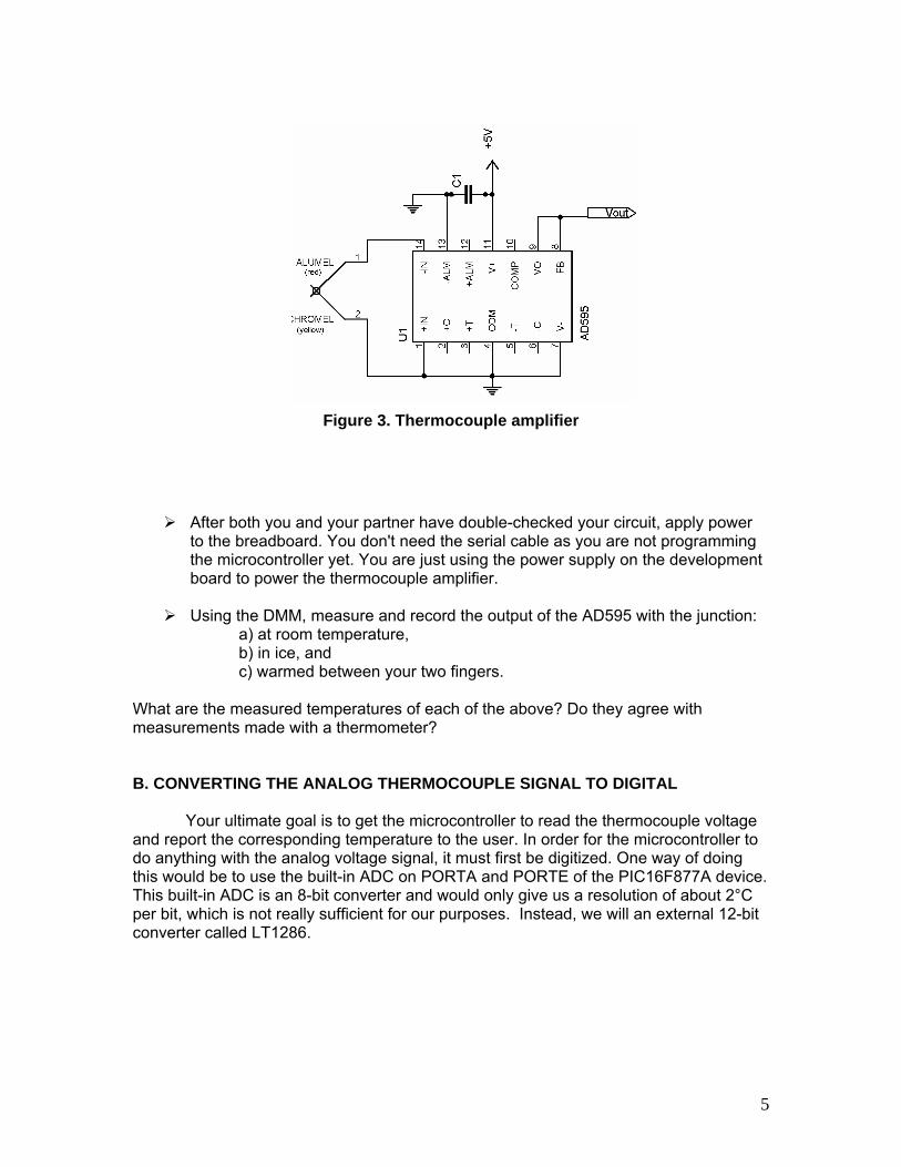
Figure 3. Thermocouple amplifier

After both you and your partner have double-checked your circuit, apply power to the breadboard. You don't need the serial cable as you are not programming the microcontroller yet. You are just using the power supply on the development board to power the thermocouple amplifier.

Using the DMM, measure and record the output of the AD595 with the junction:

a) at room temperature, b) in ice, and c) warmed between your two fingers.

What are the measured temperatures of each of the above? Do they agree with measurements made with a thermometer? B. CONVERTING THE ANALOG THERMOCOUPLE SIGNAL TO DIGITAL

Your ultimate goal is to get the microcontroller to read the thermocouple voltage and report the corresponding temperature to the user. In order for the microcontroller to do anything with the analog voltage signal, it must first be digitized. One way of doing this would be to use the built-in ADC on PORTA and PORTE of the PIC16F877A device. This built-in ADC is an 8-bit converter and would only give us a resolution of about 2°C per bit, which is not really sufficient for our purposes. Instead, we will an external 12-bit converter called LT1286.

5

The ADC circuit The circuit you will build is shown Figure 4. The thermocouple amplifier part of the circuit is the same as the one you built earlier. A few notes are in order regarding the ADC part of the circuit.

Figure 4. Analog-to-Digital Converter and Thermocouple Amplifier

1. The output of the amplifier is first filtered through a low pass filter (R2 and C2) before being sent to the input of the ADC.

2. LM285 is a 1.2 V voltage reference that behaves like a zener diode. It comes in a 3-pin package (like a transistor), but only 2 pins are used. Consult the data sheet for the proper connections. You may wish to trim off the unused pin to avoid confusion with a transistor you will use next week.

When connected as shown in Figure 4, the voltage across the reference diode is constant at about 1.2 Volts. VREF at pin 1 of the ADC sets the maximum voltage that the converter can read and it determines the resolution. For an N-bit converter, there are 2N different output levels, or 2N different binary numbers that the converter can output. Thus, there are 2N – 1 steps in the output of the converter, each step corresponding to an incremental increase in the input voltage. The resolution is sometimes defined as this incremental increase in voltage per binary step. That is, the resolution is the total voltage range divided by the number of steps, or VREF/(2N – 1). 3. A bypass capacitor, C3, is placed between the power supply (+5) and ground to reduce the amount of high frequency noise (for example, from switching and clock pulses) that might appear across the power supply. This capacitor should be placed as close as possible to the power and ground pins of the LT1286 chip. Use a 10 μF tantalum electrolytic capacitor and take care to orient it in the correct direction. The end marked with a + goes should always be more positive than the other end. Connect the + end to the V+ (pin 8) and the other end to COM (pin 4). 4. The LT1286 needs three connections to the PIC microcontroller. Two of the connections – chip select (CS) and clock (CLK) – are for pulses sent from the PIC to the ADC. The third connection is used by the ADC to send the data to the PIC. You can

6

choose almost any of the PIC I/O pins that you like for these, but you should avoid the ones used for serial communications (C6 and C7) as you will be using these to program your device.

Go ahead and build the circuit shown in Figure 4. The program You can't test your circuit without providing the analog-to-digital converter with CS and CLK signals. When it receives a falling signal at the CS (chip select) pin, it essentially wakes up and samples the data at its inputs. The clock signal (CLK) provides the timing for the conversion and transfer of data. (The sequence of events is illustrated in Figure 1 on page 10 of the LT1286 data sheet.) After the second clock pulse, the ADC outputs a null bit and the actual data transfer begins with the third pulse. One data bit is transferred for each clock pulse received. The ADC needs a total of 14 CLK pulses to transfer one voltage measurement – two during sampling and then another twelve for the 12 bits to be transferred. You will use the SHIFTIN instruction to read the results from the ADC. The SHIFTIN instruction takes care of both sending the clock pulses and reading the data. The syntax of the command is:

SHIFTIN DataPin, Clock Pin, Mode, [Var\Bits . . .], where "DataPin" is the pin on the microcontroller that is reading the data and "ClockPin" is the pin that is sending the clock pulses. Mode specifies if the data being received is most significant bit (MSB) or least significant bit (LSB) first. You can refer to the PicBasic Pro manual (pp. 145-7) for a complete description of all the modes. Since the ADC sends the data MSB first and transmit each bit with a falling clock pulse, you should set mode equal to 2. The final element in the SHIFTIN command specifies the name of the variable where the data should be stored and the number of bits to read from the ADC. An example of code that will read the ADC is given below. CS VAR PORTB.0 ' Variable that names pin used to send chip select signal CLK VAR PORTB.1 ' Variable that names pin used to send clock pulses DIO VAR PORTB.2 ' Variable that names pin used to read the ADCdata AD VAR WORD ' Variable to store result read by ADC CLEAR ' Initializes all variables HIGH CS ' Begin with CS high LOW CS ' Enables ADC

SHIFTIN DIO, CLK, 2, [AD\14] ' Reads in data and stores it HIGH CS ' Puts ADC in low power mode The code above uses variable names for the pins being used. This programming technique is convenient and makes your code more readable, but it is entirely optional. For instance, when you read the code (especially in a long program) "LOW CS" you can readily identify that a chip select signal is being sent. "LOW PORTB.0" would also work, but you might not remember that PORTB.0 sends the chip select signal.

7

Notice also that in the SHIFTIN command above, 14 bits of data are read in and

stored in the variable "AD". The first two bits read (the two most significant bits) are actually garbage because the ADC doesn't start sending data until the third clock pulse. However, the converter needs those first two clock pulses before it will start sending data. Specifying 14 bits ensures that enough clock pulses are sent to get all twelve bits of the data. Once the data is read, you can get rid of the two garbage bits by the following instruction:

AD = AD & %00111111111111 ' Throw away 2 most significant bits

This instruction takes the result in "AD" and performs a logical "AND" with the binary number shown. The result is then stored back in the same variable "AD".

Write a program that will enable the microcontroller to continually monitor the temperature of the thermocouple and display the A/D output on the LCD. You may start with the template program called "ADCTemplate" (see Appendix B). After opening the template, save it under a new name in your own folder. Note that the template is organized so that the main program continually loops and subroutines are executed from this main loop. Compile your program and correct any errors.

Run your program and see if it works! The ADC output should be displayed on

the LCD. You may need to add a PAUSE statement so that the display can be read more easily. You should see the output change if you warm the thermocouple junction between your fingers. Note that the ADC output does not give you the thermocouple voltage or the temperature directly, but you can calculate them from the result on the LCD display. You will need to know the exact value of the LV285 voltage reference to do this calculation. (You can measure it with the DMM.) Do your results make sense?

Monitor the ADC with the oscilloscope. Use two channels to look at both the

clock and data signals. Use the CS signal to externally trigger the scope. Adjust the scope settings so that you can see all 14 clock pulses and the data. Since digital low and high signals go from 0 to 5 V, you should expect the pulses to be 5 volts. You will probably have to remove your PAUSE statement from your program so that the signal is displayed continually on the scope. The data signal is simply the binary equivalent of the voltage signal read by the ADC. A high bit (+5 V) indicates a digital 1 and a low bit (0 volts) indicates a digital 0. Once you get the data signal, you will probably see the two or three least significant bits fluctuating quite a bit because of noise.

Sketch the waveforms in your notebook. Note the frequency of the clock pulses.

The frequency of the clock pulses depends on oscillator speed.

Record the binary value of the signal as displayed on the scope with the thermocouple at room temperature and at least one other temperature. Convert the binary numbers to millivolts and compare it to what you expect the voltage to be. You will again need the exact value of the LV285 voltage reference to do this calculation. Do the results make sense?

8

When viewing the ADC result on the LCD or the terminal, you have probably noticed that there is quite a bit of fluctuation in the measured thermocouple voltages. You can obtain a more stable result if you average several readings. Add a loop to your program that averages several readings. One way of doing this is to declare a new variable that stores the sum of consecutive ADC measurements. Then use a FOR. . .NEXT loop within the "GetData" subroutine to read the ADC result and add the result to the sum several times. After completing a certain number of loops (maybe 5 to 10), calculate the average ADC result and display that result on the LCD.

C. CONVERTING VOLTAGE TO TEMPERATURE It would be much more convenient if your program displayed the actual temperature instead of the ADC output. The mechanics of what should be a relatively simple calculation are actually somewhat complicated in PICBasic Pro. The complications occur because the compiler does only integer math and variables can be at most 16 bits. Therefore, you will be provided with the subroutine that does the calculation. The code (see Appendix C) is available in lab in the file "ConvertTemp.pbp". A brief (and probably not crystal clear!) explanation of the code is given in the comments. The code will not run alone and the various parts will need to be cut and pasted into your own program.

From within MicroCode Studio, cut and paste the variable declarations from "TempCalc.pbp" to the proper place in your program. Note that the variable that stores the ADC result has been called "AD". You can change the name to make it consistent with the rest of your program.

Cut and paste the variable initialization part into the proper place in your

program. If you have a "CLEAR" instruction in your code, these initializations should come after the "CLEAR" and not before. Be sure to enter the value of your voltage reference for "Vref" in millivolts.

Cut and past the subroutine "CalcTemp" into your program. Subroutines go after

the main loop of the program.

Add the line "GOSUB CalcTemp" to your main loop.

Modify your code so that you can display both the A/D result and the calculated temperature.

Run and test your program.

Print a copy of your final working program to submit with your report.

When you are done, do not take apart your working circuit. Disconnect the LCD, the thermocouple, and any other connections to the development board. Store your board with the intact circuit in the pink bag that the board came in and write your names on the label. Next week you will use the circuit that you built along with the switch box that you are working on to finish the microcontroller unit. When you put all the parts together, you will have created a feed-back system where the microcontroller monitors and controls the temperature of an experimental system.

9

REPORT For your report, turn in answers to the questions in "Report for Part B" when you come to lab next week. APPENDICES The following appendices are attached. Appendix A: Chromel-alumel (Type K) thermocouple reference sheet Appendix B: Program template "ADCTemplate.pbp" Appendix C: ConvertTemp.pbp – code for converting ADC result to temperature

10

Chemistry 628 University of Wisconsin-Madison Unit 3 Lab: Microcontrollers and Feedback

PART C: FEEDBACK CONTROL OF AN EXPERIMENT This lab is the final part of the Microcontroller Unit. You will now put together all the pieces that you have worked on the past couple of weeks. Last week you built a circuit and wrote the program code that monitored the temperature at a thermocouple junction. This week the thermocouple will measure the temperature of an aluminum block that has an attached heater. You will program the microcontroller to send signals to the relay in the AC switch box that you have built. The appropriate signal will cause the relay to either open (heater off) or close (heater on) depending how close the block is to a set temperature. Finally, you will investigate the use of a proportional-integral-derivative (PID) algorithm to control the temperature. EQUIPMENT From Parts A and B of lab: Microcode Studio Plus IDE and PicBasic Pro™ compiler (installed on desktop computer) Circuit built on 28/40 Dev Board from Part B of lab AC Power Adaptor (9 V, 500 mA) Serial Cable New for Part C: StampPlot Lite (installed on lab computer) Switch box (built outside of lab) 2N3904 NPN transistor Resistors (one 56 kΩ, one 4.7 kΩ) BACKGROUND

There are a number of different algorithms that are used for temperature control. A brief overview of some of these methods is given below. For more detailed explanations on the various methods, the student should consult other resources. Two references are included at the end of this document, but numerous other resources are available in addition to those listed.

The simplest type of temperature controller is the on/off variety. When the measured temperature (Tm) is less than the desired "set point" temperature (Ts), the heater is fully on and when the temperature is greater than the set point the heater if fully off. In the region very close to the set point, a "dead band" is usually chosen to account for hysteresis. For instance, if Tm < Ts the heater switches off when Tm is close to but still less than Ts, as opposed to waiting until the exact set point is actually reached. When Tm > Ts and the temperature is decreasing, the heater will turn on when Tm gets close to but is still greater than Ts. While having a "dead band" reduces the amount of overshoot and undershoot of the actual temperature, it does not eliminate it entirely.

Consequently, the temperature will tend to oscillate around the set point instead of being steady.

A better type of controller is a proportional controller, in which the controller

changes the power delivered to the heating element based on the difference between the actual temperature and the desired temperature. To improve the response, most proportional controllers turn the heater fully on or fully off when the temperature is far away from the set point, just like the simple on-off controller. However, when the temperature is within some pre-defined range of the set temperature, the proportional control takes over and adjusts the amount of power (heat) delivered depending on the difference between Ts and Tm. While it is sometimes possible to continuously vary the amount of power delivered to the heater, for higher-powered systems it is more common to turn the power fully on or fully off at short intervals (faster than the system can respond). With a given, short time interval (the cycle time), the fraction of time that the heater is on is adjusted by an amount proportional to Ts -Tm. Ideally, a system is designed so that the set point temperature is reached (meaning that the heat supplied just balances the heat losses) when the heater is on 50% of the time. The fraction of time that the heater is on is then adjusted greater or smaller within the cycle time depending on Ts -Tm. This process is often called pulse-width modulation (PWM) and is the approach that will be used in this lab.

Because proportional control is a part of the PID temperature control algorithm that you investigate, it will be helpful here to define a few terms. The cycle time (called "duration" in the program) is a short, fixed period of time (we will use 6 seconds) during which the heater will be turned on once and then turned off. The "drive" is the percentage of the cycle time that the heater is on. For drive = 50, the heater will be on for half of each cycle time (3 seconds) and off for the remainder (3 seconds) of each cycle time. For drive = 100, the heater is on for the entire time of each cycle. The "range" is a range of temperatures centered at the set point (called SetPoint in the program) over which the controller uses proportional gain. For instance, if the set point is 60oC and the range is 2oC, then the heater will be fully on for T < 59o, fully off for T > 61o, and will use proportional control when 59o < T < 61o.

The % Error is a measure of how far the measured temperature deviates from the set temperature and is calculated in our program relative to the range, as shown in Equation 1.

100xRange

TTError% ms −= (1)

The proportional gain, Kp, times the % Error determines, P, the contribution to "drive" from proportional control, as shown in Equations 2 and 3.

)Error(%x)K(P p= (2) P50PBdrive +=+= (3)

where B (called the bias) is the drive required to balance the heat losses and maintain the set point. Limits are places on "drive" so that it stays between 0 and 100, since it

2

makes no physical sense to have the heater on for a negative percentage of time or a greater than 100 % of the time.

The combination of the proportional gain and the range determines the temperature region over which proportional control has effect. A larger gain and/or smaller range will provide a more aggressive control over a narrower temperature region than a smaller gain and/or larger range.

While proportional control is a significant improvement over simple on/off control, it is not sufficient for all systems. If something is suddenly added to or removed from the load (in our case, the aluminum block) or the surrounding room temperature changes suddenly, the proportional controller reacts to maintain the set point. Depending on the conditions, a significant amount of overshoot or undershoot and oscillations can occur before the temperature again stabilizes at the set point. Another problem occurs because in real life, it is unlikely that the system will be at the set point when the drive is maintained at 50%. If it were close to ideal before a load is added, it will no longer be so after a load is added. The solution to these problems is to use PID control – a combination of proportional, integral and derivative control.

The overall equation for PID control is:

]dt

)Error(%dK[]dt)Error(%K[)]Error(%K[Bdrive dip ∫ +++= (4)

The first two terms are from Equations 2 and 3. The 3rd term is the integral of the error over time multiplied by an integral gain, Ki. This term adds up the deviation from the set point over time and corrects the drive accordingly. This term is useful when the temperature is steady but too high or too low relative to the set point. The fourth term is the derivative of the error multiplied by the derivative gain, Kd. When the temperature changes suddenly (because of the addition of a load or a gust of cold air, for instance) the derivative term is larger and contributes a greater amount to the drive in order to correct the temperature. If the contribution to the drive from the integral term is "I" and the contribution from the derivative term is "D", the equation becomes:

DIPBdrive +++= (5)

The feedback process of a temperature controller is completely analogous to the feedback of in an inverting amplifier op amp circuit. The temperature controller measures the difference between the measured and set temperatures or the "error". This error is analogous to the voltage difference that the op amp measures between its two inputs. The temperature controller takes the error and multiplies it by a gain to adjust the output of the heater. The feedback is negative because if the temperature is too great, the heater drive is reduced. If the temperature is too low, the heater drive is increased. An op amp takes the error at its inputs and multiplies it by the feedback gain which changes Vout. For the op amp circuit the feedback is also negative since a portion of Vout is fed back to the inverting input. In both cases, the output is adjusted so that the error is minimized.

3

EXPERIMENT A. Transistor Circuit and Switch Box In this section you will construct and test the transistor circuit that is the interface between the PIC microcontroller and the switch box that you have built. The circuit and program are described first and then the actual procedure is given. The circuit The switch box will be used to turn 120 VAC power on and off to a load, the heater. The relay switch in the box needs a control signal from the microcontroller to tell it when to open (power off) and close (power on). While this task could probably be accomplished by sending a HIGH or LOW signal directly to the relay (pin 4-), it is best to limit the amount of current drawn from the microcontroller I/O pin. This safety feature can be easily implemented by using the transistor switch shown in Figure 1. The circuit has the added advantage that the logic is no longer reversed. That is, without the transistor switch, a LOW signal from the microcontroller is required to close the relay and turn the heater on. With the transistor switch a HIGH signal from the microcontroller turns the heater is on.

Take care not to confuse the NPN transistor with the LM285 voltage reference that you used last week. The packages look the same, but the devices can be distinguished by the identification numbers stamped on them. Another way to avoid confusing the two parts is to trim the unused leg of the voltage reference.

Figure 1. Transistor Switch

The program The program for testing the combination transistor circuit and switch box has been written for you and is given in Appendix A. A few notes are in order regarding the program. 1. The program begins with the usual DEFINEs and configuration statement. Pin C4 has been chosen for the control signal, but you should change it to match your circuit. The control pin has been given the name "heater".

4

2. The constant "duration" is the duty cycle of the heater in msec. That is, it is the total "on" plus "off" time. Currently "duration" is set to 6000 msec, or 6 seconds. While you can change this number, 6 seconds works well for what we are doing. 3. The variable "drive" is the percentage of the duty cycle that the heater will be on. If "drive" were equal to 50, the heater would be on 50% of the "duration" time, or on for 3 seconds and then off for 3 seconds. In SwitchBoxTest.pbp, the value of drive is set manually by changing it within the code. Later, when you work with PID control, the value of "drive" will be calculated in the program and will depend on both the set point temperature and the actual temperature of the heater block. 4. The main routine, "DriveHeater" supplies a HIGH signal to turn the transistor on, which in turn closes the relay and supplies power to the heater. When the pin "heater" is brought low, the relay is open and the heater is off. 5. "Ontime" is the actual time (in msec) within each cycle that the heater will be on. Its value is calculated in the main program loop, "DriveHeater" with the statement: ontime = drive*(duration/100)

Some care must be taken in the order of operations when doing this simple calculation. The largest type of variable in PIC Basic is a WORD, which is 2 bytes, or 16 bits. The value of a word can range from 0 to 65,535 (or 216 – 1). If the result of a calculation exceeds 65,535, information is lost. For instance, if drive = 50 and duration = 6000, multiplying the two numbers should yield 300,000. However, this number is larger than can be expressed in 16 bits and only the 16 lowest bits are retained in Pic Basic. Therefore, the following statement does not work. ontime = (drive*duration)/100

Another math limitation in PIC Basic Pro is that the fractions are truncated. For instance, you might think that you can calculate "ontime" with the statement:

ontime = (drive/100)*duration

However, dividing drive = 50 by 100, yields 0 instead of 0.5. Anything after the decimal point is lost. While these math limitations may seem somewhat severe, in most cases it is not too difficult to work around them. It helps to test your calculations with a calculator to make sure that you avoid overflow (numbers too large) and fraction issues. Procedure

Go ahead and construct the switching circuit shown in Figure 1. Make the connection from the PIC to the transistor, but wait until later to make any connections to your switch box.

Start MicrcoCode Studio and open the program "SwitchBoxTest.pbp" located in

the PicControl folder. Change the pin for "heater" to the one you chose for your circuit. Save the modified program in your own folder.

5

Compile and load the program. Use the DMM to check the voltage at the

collector of the transistor has your program is running. It should be alternating between a low voltage (< 1 V) and a high voltage (about 5 V) as the program runs. If not, find and correct the problem before proceeding.

Now connect the transistor circuit to your switch box using the Jones connector

provided. You can also plug the aluminum block heater into your switch box.

Run and test the program again. You should see the neon lamp flashing with the same on/off time specified in the program. You should also feel the heater block warming up. Change the "drive" value and make sure that your circuit behaves as expected. If not, find and correct any problems before proceeding.

B. Combining Temperature Measurement and Heating the Block Last week you wrote a program that reads the temperature of a thermocouple and reports the result to an LCD. In this part you will add code to your program so that the microcontroller turns on the aluminum block heater and monitors its temperature. We begin here by combining the monitoring (GetData), displaying (LCDSummary), and heating (DriveHeater) functions. The actual control part (using PID routines) will come later. The circuit

Connect one end of the thermocouple wire (the twisted end) to the heater block and the other end to your circuit.

The program

Open your program that you used last week to read and display the output of the ADC. Copy and paste the relevant parts from the "TestSwitchBox" program into appropriate places in your ADC program.

Change the last line of the DriveHeater routine from "GOTO DriveHeater" to

"RETURN". In your main program loop, add the line "GOSUB DriveHeater".

Run and test your program until it works. The temperature reported on the LCD should change as the block warms up.

C. StampPlot Lite While monitoring the temperature with the LCD is useful, it would be even better to be able to graph the temperature as a function of time. StampPlot Lite is a freeware program that was designed to work with Parallex's Basic Stamp, which is another brand of microcontroller. Although the software was written for use with the Basic Stamp, it also works with PicBasic Pro. Since StampPlot Lite runs on your computer terminal, we will use the HSEROUT commands to send information to the plotting program.

6

From within MicroCode Studio, open the file "StampPlotCode.pbp" located in the PICControl directory. This code (shown in Appendix B) is not complete and will not run alone.

Copy the constant declaration statements to the appropriate place in your

program.

Copy the ConfigPlot routine to the place in your program where your other subroutines are (after the main program loop). This routine sets up Stamp Plot Lite and only needs to be executed once.

Add the code "GOSUB ConfigPlot" right before your main program loop. This

GOSUB does not go inside the loop. It is only called once to set up the plot parameters. Copy the PlotData routine into your program. Add the code "GOSUB PlotData" in your main program loop, somewhere after the call to CalcTemp but before the call to DriveHeater.

Compile and load your program.

Start StampPlot Lite. Check that COM1 is chosen and the baud rate is 9600.

Click the "Connect" check box. Reset the development board. You should see the temperature being plotted and increasing with time. You can adjust the temperature range that is displayed by changing the numbers in the white boxes by the y-axis and then clicking on the "Range" drop-down menu. You can also change the range in your program by changing the values of the constants "MinA" and "MaxA".

StampPlot Lite will save the data it receives in a text file called StampDat.txt. It will

also save messages that appear in the white window below the plot in a file called StampMsg.txt. Both files are stored in the C:\Program Files\StampPlot Lite directory. The program will continually append new data to these files. If you are collecting data that you might want to save, you should first click the "delete text file" and "delete message file" to clear these files before beginning data collection. After you have finished collecting the data, you should make a copy of the files with a new name in your own directory.

WARNING: DO NOT LEAVE THE FILES “StampPlotDat.txt” or “StampPlotMsg.txt” OPEN IN ANOTHER PROGRAM WHILE ACQUIRING DATA. StampPlot Lite WILL NOT BE ABLE TO SAVE THE DATA AND IT WILL NOT WARN YOU. IT WILL LET YOU CONTINUE WITH ALL YOUR TRIALS AND NOT LET YOU KNOW THAT IT ISN"T SAVING THE DATA!

Open the file "StampDat.txt" and examine the contents. The first two columns are

the date and time. The third column is the time in seconds since the last time StampPlot Lite was reset. The fourth column is the data point number. The fifth column is the actual data, in our case temperature in degrees Centigrade. The final column, which we are not using, is digital data received by the program.

Later when you are tuning your temperature controller, you will want to save the data stored in StampDat.txt (by copying the file and giving it a new name) and import it into an Excel spreadsheet so that you can examine it and plot it. The two columns that will be

7

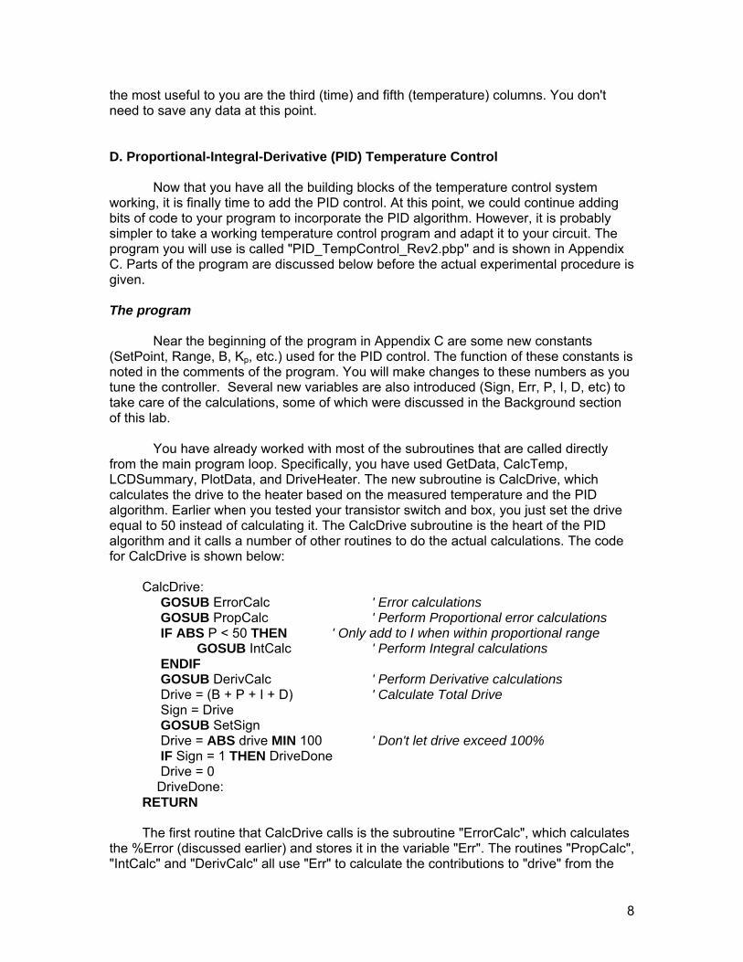
the most useful to you are the third (time) and fifth (temperature) columns. You don't need to save any data at this point.

D. Proportional-Integral-Derivative (PID) Temperature Control Now that you have all the building blocks of the temperature control system working, it is finally time to add the PID control. At this point, we could continue adding bits of code to your program to incorporate the PID algorithm. However, it is probably simpler to take a working temperature control program and adapt it to your circuit. The program you will use is called "PID_TempControl_Rev2.pbp" and is shown in Appendix C. Parts of the program are discussed below before the actual experimental procedure is given. The program

Near the beginning of the program in Appendix C are some new constants (SetPoint, Range, B, Kp, etc.) used for the PID control. The function of these constants is noted in the comments of the program. You will make changes to these numbers as you tune the controller. Several new variables are also introduced (Sign, Err, P, I, D, etc) to take care of the calculations, some of which were discussed in the Background section of this lab.

You have already worked with most of the subroutines that are called directly from the main program loop. Specifically, you have used GetData, CalcTemp, LCDSummary, PlotData, and DriveHeater. The new subroutine is CalcDrive, which calculates the drive to the heater based on the measured temperature and the PID algorithm. Earlier when you tested your transistor switch and box, you just set the drive equal to 50 instead of calculating it. The CalcDrive subroutine is the heart of the PID algorithm and it calls a number of other routines to do the actual calculations. The code for CalcDrive is shown below:

CalcDrive: GOSUB ErrorCalc ' Error calculations GOSUB PropCalc ' Perform Proportional error calculations IF ABS P < 50 THEN ' Only add to I when within proportional range GOSUB IntCalc ' Perform Integral calculations ENDIF GOSUB DerivCalc ' Perform Derivative calculations Drive = (B + P + I + D) ' Calculate Total Drive Sign = Drive GOSUB SetSign Drive = ABS drive MIN 100 ' Don't let drive exceed 100% IF Sign = 1 THEN DriveDone Drive = 0 DriveDone:

RETURN

The first routine that CalcDrive calls is the subroutine "ErrorCalc", which calculates the %Error (discussed earlier) and stores it in the variable "Err". The routines "PropCalc", "IntCalc" and "DerivCalc" all use "Err" to calculate the contributions to "drive" from the

8

proportional (P), integral (I), and derivative (D) parts of the PID algorithm, respectively. The SetSign routine is used in these routines and in CalcDrive to keep track of whether the numbers are negative or positive. A negative number will have the MSB (bit 15) of a WORD variable equal to 1, while a positive number will have the MSB equal to 0. Because of the way that PicBasic Pro handles negative numbers, the user needs to keep track of the sign of the numbers (or the value of the MSB). The SetSign routine uses the variable "Sign" to store the sign while calculations are done. Mathematical manipulations are performed on the absolute value of the number and then the sign is returned to the variable at the end of the calculation. Procedure

Make a copy of the temperature control program “PID_TempControl_Rev2.pbp” in your directory. Make the necessary changes to your program so that it works with your circuit. That is, check the TRIS instructions and change as needed. Change the pin names that are assigned to the variables CS, CLK, DIO, and Heater to reflect your pins for chip select, clock, digital out, and heater control. In the initialize variables section, change Vref to your reference value. Check the mode settings in the SEROUT2 instructions in the subroutine LCDSummary.

Investigate the proportional component of the PID algorithm. Start with a

SetPoint = 6000 (60°C), Range = 20, B = 50, Ki = Kd = 0. Try a few different values for proportional gain, such as Kp = 8, 5, and 2. Once the temperature has stabilized close to 60°C, you will see oscillations around or near the set point. Do not be concerned that the average temperature is not at the set point – it will probably be higher. This discrepancy occurs because of the inaccurate assumption made in the algorithm that when the heater is on 50% of the time, the system will be at the set point. You will fix this offset later with the integral part of the algorithm.

Your goal is to find the value of Kp that yields the smallest oscillations. You won’t eliminate them entirely until you incorporate the derivative control later. You should record the oscillations for at least 4 to 5 minutes (depending on the size of your heater block). You will need to change the y-scale in StampPlot Lite so that you can zoom in on a narrow temperature range (±1°C).

You should save your data so that you can use access it later in EXCEL. You have two options here. You can save each trial in a separate file. To do so, click "delete msg file" and "delete data file" before beginning. Then after each test, be sure to copy the files with a new name, as StampPlot Lite will reuse the original files. Alternatively, you can continually save all your data in the same file. When you read it into Excel later, you will need to find within the data where one trial ends and the next begins. If you record the start time of each trial in your notebook, you will be able to find the proper data in the data file. The advantage of the latter method is that you can look at all the data at the same time within StampPlot Lite. WARNING: DO NOT LEAVE THE FILES “StampPlotDat.txt” or “StampPlotMsg.txt” OPEN IN ANOTHER PROGRAM WHILE ACQUIRING DATA. StampPlot Lite WILL NOT BE ABLE TO SAVE ANY NEW DATA AND IT WILL NOT WARN YOU.

9

Using your optimum value of Kp, investigate how well the controller responds to a load. Place a heat sink on the block and observe how far the temperature deviates from the set point before it recovers. Save your data for later plotting and analysis.

Investigate the derivative component of the PID algorithm. You probably

noticed a rather large temperature drop in the previous step. Once the temperature has returned to the set point, wait several minutes for it to stabilize. Keeping Kp at your optimum value, try different values for the derivative gain (such as Kd = 6, 4, and 2). Your goal is to reduce both the deviation from the set temperatures and the oscillations around the set point. Notice that you can monitor the contributions to “drive” from the various gains on the LCD or the StampPlot Lite messages window.

Investigate the integral component of the PID algorithm. You probably

noticed that the average temperature achieved is not quite at the set point. Set the derivative gain back to zero and experiment with the integral gain (such as Ki = 4, 2 and 1). The integral component of the algorithm adds up the deviation from the set point over time and makes a correction based on the offset. The program is written so that the integral gain will only have an effect close to the set point. With the optimal integral gain, the stable temperature should no longer be offset from the set point.

Combine all three components – proportional, derivative, and integral – to

optimize your heater. A properly tuned controller will maintain the temperature at the set point, have a minimum of oscillations, and will recover quickly from a disturbance. Test your controller with your optimized settings to prove that it recovers quickly to an added load. If there is time, check how well the tuned heater responds when a different set point is chosen.

REPORT

The report for this lab will not be in the report sheet format that we have been using thus far. Instead, you should summarize and discuss what you observed during each part of tuning the PID temperature controller. (You do not need to describe the circuit, the experimental set-up, or the PID program itself in your report.) You should include plots from each step of the tuning process that demonstrate the effects of changing Kp, Ki, and Kd and you should discuss and explain the results. You should also include plots and discussion that demonstrate how the controller responded to a load with the various settings that you used. Finally, if you were able to determine the optimum settings, include the plot(s) and a discussion on the optimized conditions. An optimized controller should have a minimum of oscillations, a temperature at the set point, and a reasonably quick recovery from a disturbance with a minimum of overshoot and undershoot.

If your data does not clearly demonstrate the effects of each of the gains

(proportional, integral and derivative), describe what results you think you should have seen and discuss reasons for the discrepancies.

10

REFERENCES 1. Omega Engineering technical reference web page: http://www.omega.com/techref/ Omega Engineering sells a wide variety of measurement and control equipment. Their technical reference web page has numerous links to information on temperature measurement and control. The information on thermocouples is especially good. You can also get a good introduction to PID from some of the links, but a lot of the information on tuning a PID controller is specific to the products that Omega sells. 2. School of Physics at the University of Exeter web page: http://newton.ex.ac.uk/teaching/CDHW/Feedback/ This web page provides a PID tutorial for engineering students at the University of Exeter. The diagram used can be somewhat confusing for non-engineers and the tutorial uses a slightly different (but equivalent) form of the PID equation than used in this lab. However, the qualitative discussion in the tutorial is very good.

11