Addressing Non-linear Hardware Limitations and Extending Network Coverage Area for Power Aware Wireless Sensor Networks 1

Addressing Non-linear Hardware Limitations and Extending Network Coverage Area for Power Aware Wireless Sensor Networks

Michael Walsh and Martin Hayes

1

Addressing Non-linear Hardware Limitations and Extending Network Coverage Area for

Power Aware Wireless Sensor Networks

Michael Walsh1 and Martin Hayes2 1CLARITY: Centre for Sensor Web Technologies

Tyndall National Institute, University College Cork,

Cork, Ireland, 2University of Limerick

Limerick, Ireland

1. Introduction

Heterogeneous Wireless Sensor Network (WSN) technology will soon emerge from the research laboratories around the world and become embedded in everyday life. Here it will actuate, sample and organize at a scale previously thought impossible. WSNs offer an alternative to the wired communications network or can be deployed rapidly in a previously un-serviced area where they provide the ability to observe physical phenomena at a fine resolution over large spatio-temporal scales. A wireless sensor is in essence a miniature computer which can be placed anywhere or attached to anything. Typically it is powered by a battery that should be small and ideally need replacement as infrequently as possible. These ubiquitous or pervasive devices are typically in-expensive, miniature, and capable of independent computation, communication and sensing. Continuing improvements in affordable and efficient integrated electronics is having a considerable impact on the technology, that can underpin the sensor network itself and to that end, a number of state of the art sensor node platforms are now readily available. The WSN can be viewed in two ways, firstly as a decentralised group of wireless sensor nodes each limited in terms of memory, computation and functionality. Alternatively and as is more commonly the case, a WSN can be viewed as the sum of its parts. The addition of nodes to a network therefore increases the overall capabilities of the network, while the distributed manner in which these nodes are added allows the network to retain its ability to self-heal and organise. The application space for WSNs is quite large and continues to expand vigorously encompassing habitat, ecosystem, seismic and industrial process monitoring, security and surveillance as well as rapid emergency response and wellness maintenance. This unsurprisingly has generated significant attention within the research community where the question of performance robustness and optimisation appears to be a recurring theme. The

1

www.intechopen.com

engineer is therefore presented with many challenges when designing an effective deployment.

2. Wireless Sensor Network Challenges

There are numerous challenges that must be addressed when designing a WSN. There follows a brief look at a number of problems, general in the wireless context, to which systems science can provide a useful solution.

2.1 Reliable Quality of Service In a survey carried out amongst possible users of industrial wireless technology (IMS Research, 2006), 43% of the surveyed suggested that communications reliability was a major barrier to the uptake of wireless solutions in industry. The provision for Quality of Service (QoS) is therefore a key requirement if any form of WSN market penetration is to be generated. QoS has a number of different associated meanings (Goldsmith, 2006; Rappaport, 2002). In this work, QoS is taken, where specified, to imply one or both of the following

1. QoS implies that the transmitted signal will exhibit certain minimum signal strength at the receiver. This in turn will guarantee pre-specified levels of Bit Error Rate (BER) and improve demodulation at the point of access.

2. System connectivity must be ensured under the assumption that the communication link will be severed if some reliable measurable link quality metric falls below a minimum threshold value. Below this threshold the QoS is deemed unacceptable in terms of BER and the associated probability of outage in service.

2.2 Energy Efficiency Although some guaranteed level of QoS is a clear necessity, for service provision issues such as energy consumption, battery life and size are proving to be important factors when it comes to increasing the uptake of new WSN systems. Placing an upper bound on power consumption in order to maximise operational longevity is therefore also a requirement. This poses a difficult challenge as many factors can contribute to energy consumption for any given WSN deployment. However one suggestion was made in (Otto et al., 2006) where empirical evidence attributed 95% of the overall energy consumed by a wireless sensor node to communication. To narrow the focus further it was highlighted in (Zurita Ares et al., 2007) that 70% of the energy consumed by widely available WSN platforms is as a result of data transmission alone. It therefore stands to reason that minimising the time spent transmitting or optimising transceiver output power can aid greatly in energy efficiency.

2.3 Network Coverage Area In (Mobihealthnews, 2009) it was suggested that wireless networks in healthcare applications need to perform to “mission critical perfection”, where the end user must have no concerns over network coverage. It was highlighted that real service should not be “homebound” in nature but rather some level of ambulatory motion must be provided, without any technical concerns about information loss being a factor. As WSN technology is for the most part a low range solution, some design consideration must be given to provision for the need to extend network coverage area. A multi-hop hierarchy is a clear

solution to this problem, however when mobility is considered the need for handoff is introduced as a by-product. Whether it is between access points within a network or between networks, handoff must appear seamless to the user and the service must where possible remain uninterrupted.

2.4 Hardware Constraints Practical limitations are a feature of any WSN. Without exception each wireless technology is bandwidth limited and is therefore prone to congestion under heavy workloads. However empirical evidence would suggest that hardware limitations will inevitably become a factor prior to the impingement of bandwidth constraints. For instance, the IEEE 802.15.4 standard specified at 2.4 GHz supports a bandwidth of 250 kbps (IEEE 802.15.4 Standard, 2006). However, the state-of-the-art 802.15.4 compliant Tmote Sky platform can achieve only 125 kbps maximum upload and 150 kbps download over the air, as a result of microcontroller process saturation (Polastre, 2005). Other practical hardware constraints must also be considered. Transceiver output power limitations are an omnipresent feature of the WSN device. This nonlinearity can severely degrade network performance when encountered and can potentially destabilize the system entirely. Quantisation is also invariably present in a wireless communications system. Generally, a radio transceiver has a discrete number of output power levels and switching between these levels introduces unwanted quantisation noise into the system. This undesirable additional noise signal can impact negatively on communications quality. While each of these constraints is unavoidable, in practice, it is vital that their negative impact on the communication quality should be limited in an efficient manner.

3. A Solution in Systems Science

This work proposes a number of novel systems science based solutions tackling the challenges outlined above. The wireless architecture illustrated in Fig. 1 is envisaged. The IEEE 802.15.4 standard is referred to throughout as a benchmark technology, although each of the proposed methodologies presented is extendable to the general case.

Fig. 1. Envisaged Wireless Sensor Network Architecture

www.intechopen.com

Addressing Non-linear Hardware Limitations and Extending Network Coverage Area for Power Aware Wireless Sensor Networks 3

engineer is therefore presented with many challenges when designing an effective deployment.

2. Wireless Sensor Network Challenges

There are numerous challenges that must be addressed when designing a WSN. There follows a brief look at a number of problems, general in the wireless context, to which systems science can provide a useful solution.

2.1 Reliable Quality of Service In a survey carried out amongst possible users of industrial wireless technology (IMS Research, 2006), 43% of the surveyed suggested that communications reliability was a major barrier to the uptake of wireless solutions in industry. The provision for Quality of Service (QoS) is therefore a key requirement if any form of WSN market penetration is to be generated. QoS has a number of different associated meanings (Goldsmith, 2006; Rappaport, 2002). In this work, QoS is taken, where specified, to imply one or both of the following

1. QoS implies that the transmitted signal will exhibit certain minimum signal strength at the receiver. This in turn will guarantee pre-specified levels of Bit Error Rate (BER) and improve demodulation at the point of access.

2. System connectivity must be ensured under the assumption that the communication link will be severed if some reliable measurable link quality metric falls below a minimum threshold value. Below this threshold the QoS is deemed unacceptable in terms of BER and the associated probability of outage in service.

2.2 Energy Efficiency Although some guaranteed level of QoS is a clear necessity, for service provision issues such as energy consumption, battery life and size are proving to be important factors when it comes to increasing the uptake of new WSN systems. Placing an upper bound on power consumption in order to maximise operational longevity is therefore also a requirement. This poses a difficult challenge as many factors can contribute to energy consumption for any given WSN deployment. However one suggestion was made in (Otto et al., 2006) where empirical evidence attributed 95% of the overall energy consumed by a wireless sensor node to communication. To narrow the focus further it was highlighted in (Zurita Ares et al., 2007) that 70% of the energy consumed by widely available WSN platforms is as a result of data transmission alone. It therefore stands to reason that minimising the time spent transmitting or optimising transceiver output power can aid greatly in energy efficiency.

2.3 Network Coverage Area In (Mobihealthnews, 2009) it was suggested that wireless networks in healthcare applications need to perform to “mission critical perfection”, where the end user must have no concerns over network coverage. It was highlighted that real service should not be “homebound” in nature but rather some level of ambulatory motion must be provided, without any technical concerns about information loss being a factor. As WSN technology is for the most part a low range solution, some design consideration must be given to provision for the need to extend network coverage area. A multi-hop hierarchy is a clear

solution to this problem, however when mobility is considered the need for handoff is introduced as a by-product. Whether it is between access points within a network or between networks, handoff must appear seamless to the user and the service must where possible remain uninterrupted.

2.4 Hardware Constraints Practical limitations are a feature of any WSN. Without exception each wireless technology is bandwidth limited and is therefore prone to congestion under heavy workloads. However empirical evidence would suggest that hardware limitations will inevitably become a factor prior to the impingement of bandwidth constraints. For instance, the IEEE 802.15.4 standard specified at 2.4 GHz supports a bandwidth of 250 kbps (IEEE 802.15.4 Standard, 2006). However, the state-of-the-art 802.15.4 compliant Tmote Sky platform can achieve only 125 kbps maximum upload and 150 kbps download over the air, as a result of microcontroller process saturation (Polastre, 2005). Other practical hardware constraints must also be considered. Transceiver output power limitations are an omnipresent feature of the WSN device. This nonlinearity can severely degrade network performance when encountered and can potentially destabilize the system entirely. Quantisation is also invariably present in a wireless communications system. Generally, a radio transceiver has a discrete number of output power levels and switching between these levels introduces unwanted quantisation noise into the system. This undesirable additional noise signal can impact negatively on communications quality. While each of these constraints is unavoidable, in practice, it is vital that their negative impact on the communication quality should be limited in an efficient manner.

3. A Solution in Systems Science

This work proposes a number of novel systems science based solutions tackling the challenges outlined above. The wireless architecture illustrated in Fig. 1 is envisaged. The IEEE 802.15.4 standard is referred to throughout as a benchmark technology, although each of the proposed methodologies presented is extendable to the general case.

Fig. 1. Envisaged Wireless Sensor Network Architecture

www.intechopen.com

A layered approach is adopted where the goal is to exploit fully the hardware and software capabilities of the employed technology, to improve the overall service to the user. This is achieved by firstly providing suitable hardware abstractions completely exposing the functionality of the WSN hardware devices. This functionality is presented to the upper layers in the form of simple function calls. Systems science based middleware solutions are then proposed utilizing the hardware abstraction. In this regard, robust dynamic power and handoff schemes are designed and implemented on a fully compliant 802.15.4 benchmark testbed. Quantifiable improvements are reported in terms of QoS, energy efficiency and network coverage. The emphasis is placed on modularity where code reuse is encouraged sparing valuable network resources.

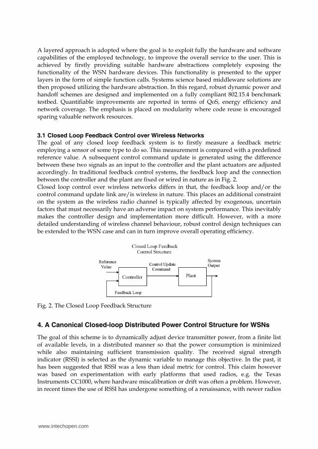
3.1 Closed Loop Feedback Control over Wireless Networks The goal of any closed loop feedback system is to firstly measure a feedback metric employing a sensor of some type to do so. This measurement is compared with a predefined reference value. A subsequent control command update is generated using the difference between these two signals as an input to the controller and the plant actuators are adjusted accordingly. In traditional feedback control systems, the feedback loop and the connection between the controller and the plant are fixed or wired in nature as in Fig. 2. Closed loop control over wireless networks differs in that, the feedback loop and/or the control command update link are/is wireless in nature. This places an additional constraint on the system as the wireless radio channel is typically affected by exogenous, uncertain factors that must necessarily have an adverse impact on system performance. This inevitably makes the controller design and implementation more difficult. However, with a more detailed understanding of wireless channel behaviour, robust control design techniques can be extended to the WSN case and can in turn improve overall operating efficiency.

Fig. 2. The Closed Loop Feedback Structure

4. A Canonical Closed-loop Distributed Power Control Structure for WSNs

The goal of this scheme is to dynamically adjust device transmitter power, from a finite list of available levels, in a distributed manner so that the power consumption is minimized while also maintaining sufficient transmission quality. The received signal strength indicator (RSSI) is selected as the dynamic variable to manage this objective. In the past, it has been suggested that RSSI was a less than ideal metric for control. This claim however was based on experimentation with early platforms that used radios, e.g. the Texas Instruments CC1000, where hardware miscalibration or drift was often a problem. However, in recent times the use of RSSI has undergone something of a renaissance, with newer radios

such as the 802.15.4 compliant TI CC2420 exhibiting highly stable performance. For example, in (Srinivasan and Levis, 2006), RSSI was proven to exhibit quite insignificant time variability as long as it stayed above an a priori defined threshold level. Recent empirical evidence would also suggest this to be the case (Alavi et al., 2008; Walsh et al., 2008; Walsh et al., 2009).

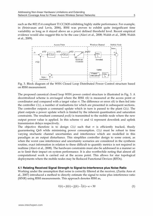
Fig. 3. Block diagram of the WSN Closed Loop Distributed Power Control structure based on RSSI measurement. The proposed canonical closed loop WSN power control structure is illustrated in Fig. 3. A decentralized scheme is envisaged where the RSSI r(k) is measured at the access point or coordinator and compared with a target value rt. The difference or error e(k) is then fed into the controller C(z), a number of realisations for which are presented in subsequent sections. The controller outputs a command update which in turn is passed to the plant G(z). The plant outputs a power update which is limited by the inherent quantisation and saturation constraints. The resultant command pm(k) is transmitted to the mobile node where the new output power value is applied. In this scheme 1 and 2 represent downlink and uplink transmission delays respectively. The objective therefore is to design C(z) such that rt is efficiently tracked, thusly guaranteeing QoS while minimising power consumption. C(z) must be robust to time varying stochastic channel uncertainties and interference which are modelled in this paradigm as an output disturbance. This simplifies controller design to some extent, as when the worst case interference and uncertainty scenarios are considered in the synthesis routine, exact information in relation to these difficult to quantify metrics is not required in realtime (Alavi et al., 2008). The hardware constraints must also be addressed in a manner so as to limit their impact on system performance. It is also worthwhile noting that almost all computational work is carried out at the access point. This allows for star topological deployments where the mobile nodes may be Reduced Functional Devices (RFDs).

4.1 Relating Received Signal Strength to Signal-to-Interference plus Noise Ratio Working under the assumption that noise is correctly filtered at the receiver, (Zurita Ares et al., 2007) introduced a method to directly estimate the signal to noise plus interference ratio (SINR) using RSSI measurements. This approach denotes RSSI as,

30)()()()( kIkgkpkr (1)

www.intechopen.com

Addressing Non-linear Hardware Limitations and Extending Network Coverage Area for Power Aware Wireless Sensor Networks 5

A layered approach is adopted where the goal is to exploit fully the hardware and software capabilities of the employed technology, to improve the overall service to the user. This is achieved by firstly providing suitable hardware abstractions completely exposing the functionality of the WSN hardware devices. This functionality is presented to the upper layers in the form of simple function calls. Systems science based middleware solutions are then proposed utilizing the hardware abstraction. In this regard, robust dynamic power and handoff schemes are designed and implemented on a fully compliant 802.15.4 benchmark testbed. Quantifiable improvements are reported in terms of QoS, energy efficiency and network coverage. The emphasis is placed on modularity where code reuse is encouraged sparing valuable network resources.

3.1 Closed Loop Feedback Control over Wireless Networks The goal of any closed loop feedback system is to firstly measure a feedback metric employing a sensor of some type to do so. This measurement is compared with a predefined reference value. A subsequent control command update is generated using the difference between these two signals as an input to the controller and the plant actuators are adjusted accordingly. In traditional feedback control systems, the feedback loop and the connection between the controller and the plant are fixed or wired in nature as in Fig. 2. Closed loop control over wireless networks differs in that, the feedback loop and/or the control command update link are/is wireless in nature. This places an additional constraint on the system as the wireless radio channel is typically affected by exogenous, uncertain factors that must necessarily have an adverse impact on system performance. This inevitably makes the controller design and implementation more difficult. However, with a more detailed understanding of wireless channel behaviour, robust control design techniques can be extended to the WSN case and can in turn improve overall operating efficiency.

Fig. 2. The Closed Loop Feedback Structure

4. A Canonical Closed-loop Distributed Power Control Structure for WSNs

The goal of this scheme is to dynamically adjust device transmitter power, from a finite list of available levels, in a distributed manner so that the power consumption is minimized while also maintaining sufficient transmission quality. The received signal strength indicator (RSSI) is selected as the dynamic variable to manage this objective. In the past, it has been suggested that RSSI was a less than ideal metric for control. This claim however was based on experimentation with early platforms that used radios, e.g. the Texas Instruments CC1000, where hardware miscalibration or drift was often a problem. However, in recent times the use of RSSI has undergone something of a renaissance, with newer radios

such as the 802.15.4 compliant TI CC2420 exhibiting highly stable performance. For example, in (Srinivasan and Levis, 2006), RSSI was proven to exhibit quite insignificant time variability as long as it stayed above an a priori defined threshold level. Recent empirical evidence would also suggest this to be the case (Alavi et al., 2008; Walsh et al., 2008; Walsh et al., 2009).

Fig. 3. Block diagram of the WSN Closed Loop Distributed Power Control structure based on RSSI measurement. The proposed canonical closed loop WSN power control structure is illustrated in Fig. 3. A decentralized scheme is envisaged where the RSSI r(k) is measured at the access point or coordinator and compared with a target value rt. The difference or error e(k) is then fed into the controller C(z), a number of realisations for which are presented in subsequent sections. The controller outputs a command update which in turn is passed to the plant G(z). The plant outputs a power update which is limited by the inherent quantisation and saturation constraints. The resultant command pm(k) is transmitted to the mobile node where the new output power value is applied. In this scheme 1 and 2 represent downlink and uplink transmission delays respectively. The objective therefore is to design C(z) such that rt is efficiently tracked, thusly guaranteeing QoS while minimising power consumption. C(z) must be robust to time varying stochastic channel uncertainties and interference which are modelled in this paradigm as an output disturbance. This simplifies controller design to some extent, as when the worst case interference and uncertainty scenarios are considered in the synthesis routine, exact information in relation to these difficult to quantify metrics is not required in realtime (Alavi et al., 2008). The hardware constraints must also be addressed in a manner so as to limit their impact on system performance. It is also worthwhile noting that almost all computational work is carried out at the access point. This allows for star topological deployments where the mobile nodes may be Reduced Functional Devices (RFDs).

4.1 Relating Received Signal Strength to Signal-to-Interference plus Noise Ratio Working under the assumption that noise is correctly filtered at the receiver, (Zurita Ares et al., 2007) introduced a method to directly estimate the signal to noise plus interference ratio (SINR) using RSSI measurements. This approach denotes RSSI as,

30)()()()( kIkgkpkr (1)

www.intechopen.com

where )(kr is the RSSI value, )(kp and )(kg are output power and attenuation respectively

and )(kI contains path-loss, shadowing, fading, interference and noise. The addition of the scalar term 30 accounts for the conversion from dBm to dB and is the measurement offset determined empirically to be 45 dB. From (Zurita Ares et al., 2007) the SINR )(k , in terms of RSSI can be described as,

30)()( krk (2)

This relationship is useful for a number of reasons. Firstly expressing RSSI in terms of SINR which in turn can be related to PER, is a suitable means of guaranteeing pre-specified levels of QoS in the closed loop system. To expand a target or reference RSSI value can be selected and related directly to PER, as outlined in the 802.15.4 standard (IEEE 802.15.4 Standard, 2006). The bit error rate (BER) for the 802.15.4 standard operating at a frequency of 2.4GHz is given by,

16

2

)11(20161

161

158

k

kSINRk e

kBER (3)

and given the average packet length for this standard is 22 bytes, the PER can be obtained from,

PLBERPER )1(1 (4)

where PL is packet length including the header and payload. PER is more useful here given the transceiver used to practically implement the proposed methodology, is a wideband transceiver, transmitting and receiving data in packet rather then bit format. Establishing a relationship between RSSI, SINR, BER and subsequently PER can therefore help to pre-specify levels of system performance. The relationship can also be used for comparative purposes, given control algorithms employing SINR, as a feedback metric can be directly applied to the WSN closed loop power control structure in Fig. 3. This is a useful tool in evaluating the performance of the proposed power control solution that follows.

4.2 Practical Hardware Limitations Practical hardware limitations are a feature of any hardware platform and can result in severe performance degradation if not handled correctly. Addressing these constraints in parallel with improving reliability and power awareness is therefore a worthwhile endeavour.

Fig. 4. Transceiver Output Power Saturation Nonlinearity

There is a maximum and minimum power at which any transceiver can transmit. These limits introduce a nonlinear saturation element to the system. The saturation nonlinearity sat(.) is illustrated in Fig. 4 and can be represented by equation (5).

(5) Without exception, there are also constraints placed on the system by the discrete nature of a transceiver's power levels. The impact switching between each discrete power level can adversely affect system performance as quantisation error is introduced. This additional input is normally modelled as noise. Generally, this signal is small in magnitude when compared with the channel variation associated with propagation effects; however it should be considered in any effective control design solution. The quantization and saturation nonlinearities are illustrated in Fig. 5.

Fig. 5. Transceiver Output Quantisation Nonlinearity

Fig. 6. The Anti-Windup approach as it applies to the Wireless Sensor Network Power Control Problem

www.intechopen.com

Addressing Non-linear Hardware Limitations and Extending Network Coverage Area for Power Aware Wireless Sensor Networks 7

where )(kr is the RSSI value, )(kp and )(kg are output power and attenuation respectively

and )(kI contains path-loss, shadowing, fading, interference and noise. The addition of the scalar term 30 accounts for the conversion from dBm to dB and is the measurement offset determined empirically to be 45 dB. From (Zurita Ares et al., 2007) the SINR )(k , in terms of RSSI can be described as,

30)()( krk (2)

This relationship is useful for a number of reasons. Firstly expressing RSSI in terms of SINR which in turn can be related to PER, is a suitable means of guaranteeing pre-specified levels of QoS in the closed loop system. To expand a target or reference RSSI value can be selected and related directly to PER, as outlined in the 802.15.4 standard (IEEE 802.15.4 Standard, 2006). The bit error rate (BER) for the 802.15.4 standard operating at a frequency of 2.4GHz is given by,

16

2

)11(20161

161

158

k

kSINRk e

kBER (3)

and given the average packet length for this standard is 22 bytes, the PER can be obtained from,

PLBERPER )1(1 (4)

where PL is packet length including the header and payload. PER is more useful here given the transceiver used to practically implement the proposed methodology, is a wideband transceiver, transmitting and receiving data in packet rather then bit format. Establishing a relationship between RSSI, SINR, BER and subsequently PER can therefore help to pre-specify levels of system performance. The relationship can also be used for comparative purposes, given control algorithms employing SINR, as a feedback metric can be directly applied to the WSN closed loop power control structure in Fig. 3. This is a useful tool in evaluating the performance of the proposed power control solution that follows.

4.2 Practical Hardware Limitations Practical hardware limitations are a feature of any hardware platform and can result in severe performance degradation if not handled correctly. Addressing these constraints in parallel with improving reliability and power awareness is therefore a worthwhile endeavour.

Fig. 4. Transceiver Output Power Saturation Nonlinearity

There is a maximum and minimum power at which any transceiver can transmit. These limits introduce a nonlinear saturation element to the system. The saturation nonlinearity sat(.) is illustrated in Fig. 4 and can be represented by equation (5).

(5) Without exception, there are also constraints placed on the system by the discrete nature of a transceiver's power levels. The impact switching between each discrete power level can adversely affect system performance as quantisation error is introduced. This additional input is normally modelled as noise. Generally, this signal is small in magnitude when compared with the channel variation associated with propagation effects; however it should be considered in any effective control design solution. The quantization and saturation nonlinearities are illustrated in Fig. 5.

Fig. 5. Transceiver Output Quantisation Nonlinearity

Fig. 6. The Anti-Windup approach as it applies to the Wireless Sensor Network Power Control Problem

www.intechopen.com

5. An Anti-Windup solution to Robust Power Control

Consider a WSN implementing power control in a distribute manner and subject to practical hardware limitations as per any deployment of this nature. The focus here is placed on assessing the effect that the limited power transmission capabilities of a typical mobile node, within a practical sensor network, will have on performance. These natural hardware constraints will impose saturation type limits that will obviously severely degrade network performance. In this chapter, a two step Anti-Windup (AW) design procedure is introduced to tackle this problem. The first step is to design a linear controller, ignoring the inherent nonlinear constraints that are placed on the system that uses a Quantitative Feedback Theory (QFT) approach to provide both robust stability and nominal performance in the linear region of operation. A feature of this first step is that it naturally bounds the time domain response of the system for a particular power level and provides a basis for assessing how a change in the quantisation noise caused by power level selection will affect performance. The second step, shown in Fig. 6, incorporates recent advances in AW theory to minimize performance degradation in the face of actuator constraints.

5.1 The Simplified System Model A systems science representation of a single access point communicating to a single mobile node is illustrated in Fig. 7. The system has reference input r(k) (reference RSSI), the value for which is determined using (2), (3) and (4) above, guaranteeing a predefined PER. q(k) is quantization noise introduced as a result of switching between discrete power levels. The controller K(z) has controller output u(k) and takes the form K(z) = [K1(z) K2(z)], a standard two degree of freedom structure.

Fig. 7. Wireless System Model with saturation block at the output. The plant G(z) is represented by G(z) = [G1(z) G2(z)], where G1(z) and G2(z) are the disturbance feedforward and feedback parts of G(z) respectively. Given no structured disturbance model is available in the form of a transfer function, G1(z) is taken to be G1 = I, where I is the identity matrix. The approach adopted regard to modelling G2(z) is similar to that suggested by (Gunnarsson et al., 1999) where the plant model for the WSN device is no longer represented by an integrator. However, rather than replace the plant model with a direct feedthrough term, (i.e., for a device G and power command update pi, the plant output is G(pi) = pi), the plant is herein modelled as a low pass filter possessed of sufficient available bandwidth to be robust to a particular level of quantization noise. G2(z) is therefore selected as,

9.01.11)(2

zzG (6)

G2(z) outputs a power level update p(k), which in turn is transmitted to the mobile node. The mobile node transmitter has inherent upper and lower bounds on hardware transmission power output, represented in Fig. 7 by the saturation block, the output for which is saturated output power or pm(k). H represents the hardware switch in the mobile node’s transceiver and is taken here to be the identity matrix or H = I. d(k) is a disturbance to the system and comprises of channel attenuation, interference and noise.

5.2 Mapping the Saturation Function For this scenario, a problem presents itself in that the saturation constraint is located at the output of the system and while there have been some advances in control design theory to deal with this type of output constraint for instance (Grandhi et al., 1995; Andersin et al., 1998), there is a vast literature covering the treatment of linear systems subject to input saturation constraints, see (Bernstein and Michel, 1995) and references therein. A solution therefore lies in the mapping of the output saturation constraint to the input of the plant or the output of the controller. The saturation function is defined as,

))(()( kpsatkpm (7)

where )}(|,)(min{|))(())(( kpkpkpsignkpsat m and )(kpm is the output power saturation limit. Note the sat(.) function in (6), belongs to sector [0, 1] and is assumed locally Lipschitz. The following set is defined,

)](),([ kpkp mm (8)

where )(),())(( kpkpkpsat . This is the set in which the saturation behaves linearly i.e. if there is no saturation present )]()( kpkp m and the nominal closed loop system conditions are exhibited. Fig. 8 portrays the system with the saturation block mapped from the output of the system to the input where um(k) is the input to the plant. To represent the mapped saturation function we define the new set,

])(,)([22 G

m

G

mh

kph

kp (9)

where 2Gh is the gain of the transfer function G2. Recent advances in the antiwindup

literature can now be applied to the problem at hand, ensuring minimal performance degradation during saturation and speedy recovery following saturation.

Fig. 8. Wireless System Model with saturation block mapped from the output to the input of the system.

www.intechopen.com

Addressing Non-linear Hardware Limitations and Extending Network Coverage Area for Power Aware Wireless Sensor Networks 9

5. An Anti-Windup solution to Robust Power Control

Consider a WSN implementing power control in a distribute manner and subject to practical hardware limitations as per any deployment of this nature. The focus here is placed on assessing the effect that the limited power transmission capabilities of a typical mobile node, within a practical sensor network, will have on performance. These natural hardware constraints will impose saturation type limits that will obviously severely degrade network performance. In this chapter, a two step Anti-Windup (AW) design procedure is introduced to tackle this problem. The first step is to design a linear controller, ignoring the inherent nonlinear constraints that are placed on the system that uses a Quantitative Feedback Theory (QFT) approach to provide both robust stability and nominal performance in the linear region of operation. A feature of this first step is that it naturally bounds the time domain response of the system for a particular power level and provides a basis for assessing how a change in the quantisation noise caused by power level selection will affect performance. The second step, shown in Fig. 6, incorporates recent advances in AW theory to minimize performance degradation in the face of actuator constraints.

5.1 The Simplified System Model A systems science representation of a single access point communicating to a single mobile node is illustrated in Fig. 7. The system has reference input r(k) (reference RSSI), the value for which is determined using (2), (3) and (4) above, guaranteeing a predefined PER. q(k) is quantization noise introduced as a result of switching between discrete power levels. The controller K(z) has controller output u(k) and takes the form K(z) = [K1(z) K2(z)], a standard two degree of freedom structure.

Fig. 7. Wireless System Model with saturation block at the output. The plant G(z) is represented by G(z) = [G1(z) G2(z)], where G1(z) and G2(z) are the disturbance feedforward and feedback parts of G(z) respectively. Given no structured disturbance model is available in the form of a transfer function, G1(z) is taken to be G1 = I, where I is the identity matrix. The approach adopted regard to modelling G2(z) is similar to that suggested by (Gunnarsson et al., 1999) where the plant model for the WSN device is no longer represented by an integrator. However, rather than replace the plant model with a direct feedthrough term, (i.e., for a device G and power command update pi, the plant output is G(pi) = pi), the plant is herein modelled as a low pass filter possessed of sufficient available bandwidth to be robust to a particular level of quantization noise. G2(z) is therefore selected as,

9.01.11)(2

zzG (6)

G2(z) outputs a power level update p(k), which in turn is transmitted to the mobile node. The mobile node transmitter has inherent upper and lower bounds on hardware transmission power output, represented in Fig. 7 by the saturation block, the output for which is saturated output power or pm(k). H represents the hardware switch in the mobile node’s transceiver and is taken here to be the identity matrix or H = I. d(k) is a disturbance to the system and comprises of channel attenuation, interference and noise.

5.2 Mapping the Saturation Function For this scenario, a problem presents itself in that the saturation constraint is located at the output of the system and while there have been some advances in control design theory to deal with this type of output constraint for instance (Grandhi et al., 1995; Andersin et al., 1998), there is a vast literature covering the treatment of linear systems subject to input saturation constraints, see (Bernstein and Michel, 1995) and references therein. A solution therefore lies in the mapping of the output saturation constraint to the input of the plant or the output of the controller. The saturation function is defined as,

))(()( kpsatkpm (7)

where )}(|,)(min{|))(())(( kpkpkpsignkpsat m and )(kpm is the output power saturation limit. Note the sat(.) function in (6), belongs to sector [0, 1] and is assumed locally Lipschitz. The following set is defined,

)](),([ kpkp mm (8)

where )(),())(( kpkpkpsat . This is the set in which the saturation behaves linearly i.e. if there is no saturation present )]()( kpkp m and the nominal closed loop system conditions are exhibited. Fig. 8 portrays the system with the saturation block mapped from the output of the system to the input where um(k) is the input to the plant. To represent the mapped saturation function we define the new set,

])(,)([22 G

m

G

mh

kph

kp (9)

where 2Gh is the gain of the transfer function G2. Recent advances in the antiwindup

literature can now be applied to the problem at hand, ensuring minimal performance degradation during saturation and speedy recovery following saturation.

Fig. 8. Wireless System Model with saturation block mapped from the output to the input of the system.

www.intechopen.com

5.3 Robust Linear Power Tracking Controller Design Quantitative feedback theory (QFT) provides an intuitively appealing means of guaranteeing both robust stability and performance and is essentially a Two-Degree-of-Freedom (2DOF) frequency domain technique, as illustrated in Fig. 8. The scheme achieves client-specified levels of desired performance over a region of parametric plant uncertainty, determined a priori by the engineer. The methodology requires that the desired time-domain responses are translated into frequency domain tolerances, which in turn lead to design bounds in the loop function on the Nichols chart. In a QFT design, the responsibility of the feedback compensator, K2(z), is to focus primarily on attenuating the undesirable effects of uncertainty, disturbance and noise. Having arrived at an appropriate K2(z), a pre-filter K1(z), is then designed so as to shift the closed-loop response to the desired tracking region, again specified a priori by the engineer. The approach requires that the designer select a set of desired specifications in relation to the magnitude of the frequency response of the closed-loop system, thusly achieving robust stability and performance. The design procedure in its entirety is omitted here due to space constraints, however the interested reader is directed to (Horowitz, 2001) and references therein. Using this technique, K2(z) was found to be,

7103.07103.06622.0)(2

z

zzK (10)

guaranteeing a phase and gain margin equal to 50o and 1.44, respectively. The closed-loop transfer function is shaped using K1(z) ensuring the system achieves steady state around the target value of )(255 stss and a damping factor of = 0.5 is selected to reduce outage probability at the outset of communication. The resultant K1(z) is,

4127.04127.1)(1

zzzK (11)

5.4 Weston Postlethwaite Anti-Windup Synthesis Consider the generic AW configuration shown in Fig. 9. As illustrated above the plant takes the form G(z) = [G1(z) G2(z)], the linear controller is represented by K(z) = [K1(z) K2(z)], and = [1(z) 2(z)] is the AW controller becoming active only when saturation occurs. Given the difficulty in analyzing the stability and performance of this system we now adopt a framework first introduced in (Weston and Postlewaite, 2000) for the problem at hand. This approach reduces to a linear time invariant Anti-Windup scheme that is optimized in terms of one transfer function M(z) shown in Fig.10. It was shown by (Weston and Postlewaite, 2000) that the performance degradation experienced by the system during saturation is directly related to the mapping dlin yuT : . This may not be clear at first glance, however if one looks at the equivalent representation of the system illustrated in Fig.11 and derived in (Weston and Postlewaite, 2000), it can be seen that the decoupled system is divided into three sections: the nominal linear system, the disturbance filter and the nonlinear loop. Note that from Fig. 11, M - I is considered for the stability of T and G2M determines the system recovery after saturation. This decoupled representation clearly illustrates how this

mapping can be utilized as a performance measure for the AW controller. To quantify this an AW controller is selected such that the l2-gain, 2,iT , of the operator T,

2

2

02,

2

suplin

d

lui u

yT

lin (12)

where the l2 norm 2x of a discrete signal x(h),(h=0,1,2,3,….) is,

0

22 )(

h

hxx (13)

Fig. 9. A generic anti-windup scenario.

Fig. 10. Weston Postlethwaite Anti-Windup conditioning technique.

Fig. 11. Equivalent representation WPAW conditioning technique.

www.intechopen.com

Addressing Non-linear Hardware Limitations and Extending Network Coverage Area for Power Aware Wireless Sensor Networks 11

5.3 Robust Linear Power Tracking Controller Design Quantitative feedback theory (QFT) provides an intuitively appealing means of guaranteeing both robust stability and performance and is essentially a Two-Degree-of-Freedom (2DOF) frequency domain technique, as illustrated in Fig. 8. The scheme achieves client-specified levels of desired performance over a region of parametric plant uncertainty, determined a priori by the engineer. The methodology requires that the desired time-domain responses are translated into frequency domain tolerances, which in turn lead to design bounds in the loop function on the Nichols chart. In a QFT design, the responsibility of the feedback compensator, K2(z), is to focus primarily on attenuating the undesirable effects of uncertainty, disturbance and noise. Having arrived at an appropriate K2(z), a pre-filter K1(z), is then designed so as to shift the closed-loop response to the desired tracking region, again specified a priori by the engineer. The approach requires that the designer select a set of desired specifications in relation to the magnitude of the frequency response of the closed-loop system, thusly achieving robust stability and performance. The design procedure in its entirety is omitted here due to space constraints, however the interested reader is directed to (Horowitz, 2001) and references therein. Using this technique, K2(z) was found to be,

7103.07103.06622.0)(2

z

zzK (10)

guaranteeing a phase and gain margin equal to 50o and 1.44, respectively. The closed-loop transfer function is shaped using K1(z) ensuring the system achieves steady state around the target value of )(255 stss and a damping factor of = 0.5 is selected to reduce outage probability at the outset of communication. The resultant K1(z) is,

4127.04127.1)(1

zzzK (11)

5.4 Weston Postlethwaite Anti-Windup Synthesis Consider the generic AW configuration shown in Fig. 9. As illustrated above the plant takes the form G(z) = [G1(z) G2(z)], the linear controller is represented by K(z) = [K1(z) K2(z)], and = [1(z) 2(z)] is the AW controller becoming active only when saturation occurs. Given the difficulty in analyzing the stability and performance of this system we now adopt a framework first introduced in (Weston and Postlewaite, 2000) for the problem at hand. This approach reduces to a linear time invariant Anti-Windup scheme that is optimized in terms of one transfer function M(z) shown in Fig.10. It was shown by (Weston and Postlewaite, 2000) that the performance degradation experienced by the system during saturation is directly related to the mapping dlin yuT : . This may not be clear at first glance, however if one looks at the equivalent representation of the system illustrated in Fig.11 and derived in (Weston and Postlewaite, 2000), it can be seen that the decoupled system is divided into three sections: the nominal linear system, the disturbance filter and the nonlinear loop. Note that from Fig. 11, M - I is considered for the stability of T and G2M determines the system recovery after saturation. This decoupled representation clearly illustrates how this

mapping can be utilized as a performance measure for the AW controller. To quantify this an AW controller is selected such that the l2-gain, 2,iT , of the operator T,

2

2

02,

2

suplin

d

lui u

yT

lin (12)

where the l2 norm 2x of a discrete signal x(h),(h=0,1,2,3,….) is,

0

22 )(

h

hxx (13)

Fig. 9. A generic anti-windup scenario.

Fig. 10. Weston Postlethwaite Anti-Windup conditioning technique.

Fig. 11. Equivalent representation WPAW conditioning technique.

www.intechopen.com

5.5 Static anti-windup synthesis Static AW has an advantage in that it can be implemented at a much lower computational cost and adds no additional states to the closed loop system. Full order AW synthesis or AW with order equal to the plant will often lead to less response deterioration during saturation, however significant computation is required. This is often unacceptable, especially in systems that are of higher order and where additional states are undesirable. For this reason, it is common practice that most windup problems are suppressed using static compensators, see for example (Hanus et al., 1987). Using the aforementioned conditioning technique via M(z), outlined in (Turner and Postlethwaite 2004), from Fig. 9 is given by,

uu ˆˆ2

1

2

1

(14)

where u is derived from Figs. 9 and 10, respectively as,

uKyKrKu

uIMGKIyKrKuˆ)(

ˆ])[(

12221

2221

(15)

Thus, M(z) can be written as,

)()( 1221

22 IKGKIM (16)

The goal of the static AW approach is therefore to ensure that extra modes do not appear in the system. Since this will inevitably be the case, it must be ensured that minimal realizations of the controller and plant are used (Turner and Postlethwaite 2004). A state space realization can then be formed,

ux

DDCDDCBBA

yux

zNIzM

d

d ˆ)()(

2022

1011

0

(17)

where = [1(z) 2(z)] is a static matrix and x , A , 0B , B , 1C , 01D , 1D , 2C , 02D and 2D are minimal realizations given in Appendix A. A solution is obtained for the Linear Matrix Inequality (LMI) in (18) with Q>0,U =diag(v1, . . .,vc)>0, L (c+n)×n (where c=n), and the minimized l2 gain 2,iT (where is the l2 gain bound on T). In this instance, is given

by =L−1 using which, the

0

000

''''''0''

2010

211

II

QDLUDIBLUBX

CQAQCQQ

(18)

where 101101 '''2 DLUDLDUDUX . Such an l2 design ensures that during saturation closed-loop performance is achieved by staying close to the nominal design while the time

spent in saturation is also jointly minimized. Applying this synthesis routine to our plant given by (6) and linear controller (18), the resultant controller is =[−0.2049 0.6377]’ obtained using the LMI toolbox in Matlab.

6. An Anti-Windup approach to Power Aware Seamless Handoff

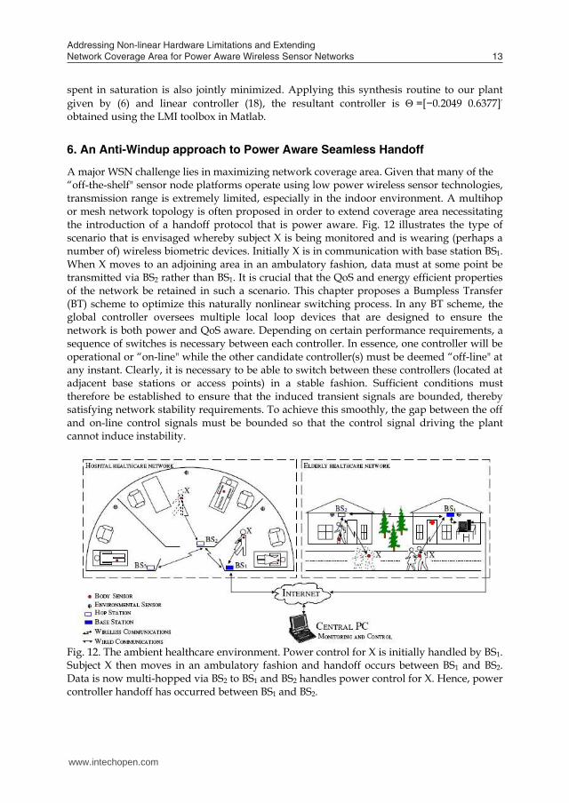
A major WSN challenge lies in maximizing network coverage area. Given that many of the “off-the-shelf" sensor node platforms operate using low power wireless sensor technologies, transmission range is extremely limited, especially in the indoor environment. A multihop or mesh network topology is often proposed in order to extend coverage area necessitating the introduction of a handoff protocol that is power aware. Fig. 12 illustrates the type of scenario that is envisaged whereby subject X is being monitored and is wearing (perhaps a number of) wireless biometric devices. Initially X is in communication with base station BS1. When X moves to an adjoining area in an ambulatory fashion, data must at some point be transmitted via BS2 rather than BS1. It is crucial that the QoS and energy efficient properties of the network be retained in such a scenario. This chapter proposes a Bumpless Transfer (BT) scheme to optimize this naturally nonlinear switching process. In any BT scheme, the global controller oversees multiple local loop devices that are designed to ensure the network is both power and QoS aware. Depending on certain performance requirements, a sequence of switches is necessary between each controller. In essence, one controller will be operational or “on-line" while the other candidate controller(s) must be deemed “off-line" at any instant. Clearly, it is necessary to be able to switch between these controllers (located at adjacent base stations or access points) in a stable fashion. Sufficient conditions must therefore be established to ensure that the induced transient signals are bounded, thereby satisfying network stability requirements. To achieve this smoothly, the gap between the off and on-line control signals must be bounded so that the control signal driving the plant cannot induce instability.

Fig. 12. The ambient healthcare environment. Power control for X is initially handled by BS1. Subject X then moves in an ambulatory fashion and handoff occurs between BS1 and BS2. Data is now multi-hopped via BS2 to BS1 and BS2 handles power control for X. Hence, power controller handoff has occurred between BS1 and BS2.

www.intechopen.com

Addressing Non-linear Hardware Limitations and Extending Network Coverage Area for Power Aware Wireless Sensor Networks 13

5.5 Static anti-windup synthesis Static AW has an advantage in that it can be implemented at a much lower computational cost and adds no additional states to the closed loop system. Full order AW synthesis or AW with order equal to the plant will often lead to less response deterioration during saturation, however significant computation is required. This is often unacceptable, especially in systems that are of higher order and where additional states are undesirable. For this reason, it is common practice that most windup problems are suppressed using static compensators, see for example (Hanus et al., 1987). Using the aforementioned conditioning technique via M(z), outlined in (Turner and Postlethwaite 2004), from Fig. 9 is given by,

uu ˆˆ2

1

2

1

(14)

where u is derived from Figs. 9 and 10, respectively as,

uKyKrKu

uIMGKIyKrKuˆ)(

ˆ])[(

12221

2221

(15)

Thus, M(z) can be written as,

)()( 1221

22 IKGKIM (16)

The goal of the static AW approach is therefore to ensure that extra modes do not appear in the system. Since this will inevitably be the case, it must be ensured that minimal realizations of the controller and plant are used (Turner and Postlethwaite 2004). A state space realization can then be formed,

ux

DDCDDCBBA

yux

zNIzM

d

d ˆ)()(

2022

1011

0

(17)

where = [1(z) 2(z)] is a static matrix and x , A , 0B , B , 1C , 01D , 1D , 2C , 02D and 2D are minimal realizations given in Appendix A. A solution is obtained for the Linear Matrix Inequality (LMI) in (18) with Q>0,U =diag(v1, . . .,vc)>0, L (c+n)×n (where c=n), and the minimized l2 gain 2,iT (where is the l2 gain bound on T). In this instance, is given

by =L−1 using which, the

0

000

''''''0''

2010

211

II

QDLUDIBLUBX

CQAQCQQ

(18)

where 101101 '''2 DLUDLDUDUX . Such an l2 design ensures that during saturation closed-loop performance is achieved by staying close to the nominal design while the time

spent in saturation is also jointly minimized. Applying this synthesis routine to our plant given by (6) and linear controller (18), the resultant controller is =[−0.2049 0.6377]’ obtained using the LMI toolbox in Matlab.

6. An Anti-Windup approach to Power Aware Seamless Handoff

A major WSN challenge lies in maximizing network coverage area. Given that many of the “off-the-shelf" sensor node platforms operate using low power wireless sensor technologies, transmission range is extremely limited, especially in the indoor environment. A multihop or mesh network topology is often proposed in order to extend coverage area necessitating the introduction of a handoff protocol that is power aware. Fig. 12 illustrates the type of scenario that is envisaged whereby subject X is being monitored and is wearing (perhaps a number of) wireless biometric devices. Initially X is in communication with base station BS1. When X moves to an adjoining area in an ambulatory fashion, data must at some point be transmitted via BS2 rather than BS1. It is crucial that the QoS and energy efficient properties of the network be retained in such a scenario. This chapter proposes a Bumpless Transfer (BT) scheme to optimize this naturally nonlinear switching process. In any BT scheme, the global controller oversees multiple local loop devices that are designed to ensure the network is both power and QoS aware. Depending on certain performance requirements, a sequence of switches is necessary between each controller. In essence, one controller will be operational or “on-line" while the other candidate controller(s) must be deemed “off-line" at any instant. Clearly, it is necessary to be able to switch between these controllers (located at adjacent base stations or access points) in a stable fashion. Sufficient conditions must therefore be established to ensure that the induced transient signals are bounded, thereby satisfying network stability requirements. To achieve this smoothly, the gap between the off and on-line control signals must be bounded so that the control signal driving the plant cannot induce instability.

Fig. 12. The ambient healthcare environment. Power control for X is initially handled by BS1. Subject X then moves in an ambulatory fashion and handoff occurs between BS1 and BS2. Data is now multi-hopped via BS2 to BS1 and BS2 handles power control for X. Hence, power controller handoff has occurred between BS1 and BS2.

www.intechopen.com

The overall solution therefore requires both AW and BT to operate in tandem for the first time in a practical WSN, thereby providing effective control of the signal entering the 'plant' (in this case the node transceiver) at any instant. For the remainder of the work, the term Anti-Windup-Bumpless-Transfer or AWBT will denote the new technique. Traditional AWBT schemes require that the gap between the feedback measurement observed at the off-line controller(s), is (are) sufficiently close in magnitude to the signal observed at the on-line controller. This is unlikely to be the case in the closed loop canonical WSN power control structure considered here as the RSSI observed at each access point will differ dramatically. To this end a specific modification is now proposed that delivers an AWBT scheme capable of compensating for the differing feedback signals that naturally arise and are unique to the wireless communications problem at hand. In the first instance, the problem is treated for a 2 base station scenario and is subsequently extended to the general case.

6.1 Formal Statement of the Handoff Problem: Two Base Station Scenario To determine when handoff should occur, the filtered downlink RSSI signal is considered at the mobile node. It is assumed that each base station or access point will transmit at a pre-defined maximum power level within some pre-defined quantization structure at any instant. Initially, a two node mobile ad-hoc WSN structure depicted in Fig. 13 is considered. When the network initializes, it is assumed that the Mobile Node (MN) is unaware of its position and is transmitting data at the maximum power level to all “listening" base stations Fig. 13(i). The network connects and implements a handoff protocol illustrated in Fig. 14. The MN will subsequently receive data packets from each base station within range (in this scenario limited to BS1 and BS2). A downlink RSSI is now calculated for each received packet and this signal is subsequently filtered to remove any multipath or high frequency component, using a digital filter, F(z). In the experiment presented in this work, the following filter was found to be satisfactory.

75.0

25.0)( z

zzF (19)

Fig. 13. Simple WSN multihop handoff scenario.

Fig. 14. The handoff procedure based on filtered downlink RSSI. Fig. 15 illustrates how, subsequent to filtering the downlink RSSI signal, the pathloss component remains. This element is shown here, (and earlier by other authors e.g. (Goldsmith, 2006)) to be sufficiently distance dependant to be a useful metric for real time control. The MN now executes the algorithm presented in Fig. 16 comparing the resultant filtered signals, RSSIDownlinkBS1 and RSSIDownlinkBS2 over three sample periods. The signals are also compared with a predefined threshold value, selected here to be -40 dBm. This threshold ensures that the base station is located in the highest possible tier of the WBAN hierarchy and is also within range of the mobile node that is currently enjoying routing precedence, thereby satisfying a minimal latency requirement within the network.

Fig. 15. Received signal strength filtered to remove the high frequency component.

www.intechopen.com

Addressing Non-linear Hardware Limitations and Extending Network Coverage Area for Power Aware Wireless Sensor Networks 15

The overall solution therefore requires both AW and BT to operate in tandem for the first time in a practical WSN, thereby providing effective control of the signal entering the 'plant' (in this case the node transceiver) at any instant. For the remainder of the work, the term Anti-Windup-Bumpless-Transfer or AWBT will denote the new technique. Traditional AWBT schemes require that the gap between the feedback measurement observed at the off-line controller(s), is (are) sufficiently close in magnitude to the signal observed at the on-line controller. This is unlikely to be the case in the closed loop canonical WSN power control structure considered here as the RSSI observed at each access point will differ dramatically. To this end a specific modification is now proposed that delivers an AWBT scheme capable of compensating for the differing feedback signals that naturally arise and are unique to the wireless communications problem at hand. In the first instance, the problem is treated for a 2 base station scenario and is subsequently extended to the general case.

6.1 Formal Statement of the Handoff Problem: Two Base Station Scenario To determine when handoff should occur, the filtered downlink RSSI signal is considered at the mobile node. It is assumed that each base station or access point will transmit at a pre-defined maximum power level within some pre-defined quantization structure at any instant. Initially, a two node mobile ad-hoc WSN structure depicted in Fig. 13 is considered. When the network initializes, it is assumed that the Mobile Node (MN) is unaware of its position and is transmitting data at the maximum power level to all “listening" base stations Fig. 13(i). The network connects and implements a handoff protocol illustrated in Fig. 14. The MN will subsequently receive data packets from each base station within range (in this scenario limited to BS1 and BS2). A downlink RSSI is now calculated for each received packet and this signal is subsequently filtered to remove any multipath or high frequency component, using a digital filter, F(z). In the experiment presented in this work, the following filter was found to be satisfactory.

75.0

25.0)( z

zzF (19)

Fig. 13. Simple WSN multihop handoff scenario.

Fig. 14. The handoff procedure based on filtered downlink RSSI. Fig. 15 illustrates how, subsequent to filtering the downlink RSSI signal, the pathloss component remains. This element is shown here, (and earlier by other authors e.g. (Goldsmith, 2006)) to be sufficiently distance dependant to be a useful metric for real time control. The MN now executes the algorithm presented in Fig. 16 comparing the resultant filtered signals, RSSIDownlinkBS1 and RSSIDownlinkBS2 over three sample periods. The signals are also compared with a predefined threshold value, selected here to be -40 dBm. This threshold ensures that the base station is located in the highest possible tier of the WBAN hierarchy and is also within range of the mobile node that is currently enjoying routing precedence, thereby satisfying a minimal latency requirement within the network.

Fig. 15. Received signal strength filtered to remove the high frequency component.

www.intechopen.com

Fig. 16. Pseudo code for handoff algorithm: 2 base station example. An admission request is then sent to the base station whose downlink RSSI satisfies the handoff criteria (BS1 following network initialization). Following receipt of a confirmation message, the mobile node implements any power level updates received from this base station. Filtering the RSSI provides the added advantage of preventing any handoff chatter, i.e., that might occur due to deep fades in the RSSI that can be a characteristic of the MN position at any instant. Furthermore, the three sample period delay prior to the transmission of an admission request ensures that jitter is not present in the system. From Fig. 12(ii) and following network initialization, MN is now located in Tier 1 of the network hierarchy and BS1, located in Tier 0, dynamically manages the MN's power based on the uplink RSSI observed at BS1. At some future sampling instant, due to MN mobility, handoff is required based on the handoff algorithm of Fig. 16, again by a consideration of the filtered downlink RSSI values, RSSIDownlinkBS1 and RSSIDownlinkBS2 and the threshold value -40 dBm. Subsequently MN joins Tier 2 in the hierarchy; see Fig. 13(iii) and a floor performance level of power control for MN should now be immediately achieved employing the uplink RSSI at BS2 as a feedback metric.

6.2 The Handoff Problem Fig. 17 illustrates a simplified handoff problem for a two base station, one mobile node scenario. KBS1 and KBS2 are two degree of freedom controllers. Initially and without loss of generality, assume base station 1 is on-line and is therefore controlling the mobile node's transmission power at the sample instant k. The problem at hand when switching is necessary between base station 1 and 2, is to avoid the jump discontinuity that may arise between p1(k) and p2(k) at the time of switching. This jump can occur due to e.g., incompatible initial conditions and can induce an unwanted transient and even instability in the system. This can lead to insufficient floor levels in the flow of information in the network. Conditions for stable Handoff: Assumption 1: Given G2 = (Ap,Bp,Cp,Dp) in state space format and that H(z) is the identity matrix, if 1)(max pA , where max is the maximum eigenvalue, then asymptotic stability

will be attained. Assumption 2: It is assumed that the poles of (1−KBS1G2H)(z) and (1−KBS2G2H)(z) are in the open unit disc, ensuring that both nominal closed loops are stable.

Fig. 17. Wireless System Model with power controller handoff. When the above two necessary conditions are met, then the stability of the switched system will be guaranteed if the control signals, um1(k) and um2(k) are sufficiently close to each other. An AWBT approach that satisfies this performance criterion therefore provides a stable solution to the handoff problem. p1(k) will be close enough to p2(k) and should handoff occur, a large potentially destabilising transient will not be induced in the system. One particular difficulty arises in the wireless case. In order that AWBT be effective, the feedback measurement observed at the off-line controller must be sufficiently close in magnitude to the feedback measurement observed by the on-line controller. Clearly from Fig. 17,

)()( 21 kdkd due to differing propagation environments. This disparity can mean AWBT will be unable to compensate for the difference between um1(k) and um2(k).

6.3 Modified Anti-Windup-Bumpless-Transfer Design The following modification compensates for the inherent discrepancy in feedback RSSI signals between the off-line and the on-line controllers. Figure 18 illustrates the modification.. Consider the off-line controller base station 2, where an additional signal ydiff2(k) is added the feedback signal. This signal is now, )()()()()( 22 zWkyzWkyky linonlinediff (20)

where W(z) is a low pass filter that removes the high frequency component present in each of the feedback RSSI signals. Note that yonline(k) is determined by which base station is on-line. Therefore yonline(k) = ylin1 when BS1 is on-line. The signal driving the off-line controller then becomes, )()()()()()()()( 212222mod zWkyzWkykykykyky linlinlindifflin

))(1)(()()()( 212mod zWkyzWkyky linlin (21) which comprises the DC or low frequency component of the on-line feedback signal or ylin1(k)W(z) plus the high frequency component of the off-line control signal ylin2(k)(1− W(z)).

www.intechopen.com

Addressing Non-linear Hardware Limitations and Extending Network Coverage Area for Power Aware Wireless Sensor Networks 17

Fig. 16. Pseudo code for handoff algorithm: 2 base station example. An admission request is then sent to the base station whose downlink RSSI satisfies the handoff criteria (BS1 following network initialization). Following receipt of a confirmation message, the mobile node implements any power level updates received from this base station. Filtering the RSSI provides the added advantage of preventing any handoff chatter, i.e., that might occur due to deep fades in the RSSI that can be a characteristic of the MN position at any instant. Furthermore, the three sample period delay prior to the transmission of an admission request ensures that jitter is not present in the system. From Fig. 12(ii) and following network initialization, MN is now located in Tier 1 of the network hierarchy and BS1, located in Tier 0, dynamically manages the MN's power based on the uplink RSSI observed at BS1. At some future sampling instant, due to MN mobility, handoff is required based on the handoff algorithm of Fig. 16, again by a consideration of the filtered downlink RSSI values, RSSIDownlinkBS1 and RSSIDownlinkBS2 and the threshold value -40 dBm. Subsequently MN joins Tier 2 in the hierarchy; see Fig. 13(iii) and a floor performance level of power control for MN should now be immediately achieved employing the uplink RSSI at BS2 as a feedback metric.

6.2 The Handoff Problem Fig. 17 illustrates a simplified handoff problem for a two base station, one mobile node scenario. KBS1 and KBS2 are two degree of freedom controllers. Initially and without loss of generality, assume base station 1 is on-line and is therefore controlling the mobile node's transmission power at the sample instant k. The problem at hand when switching is necessary between base station 1 and 2, is to avoid the jump discontinuity that may arise between p1(k) and p2(k) at the time of switching. This jump can occur due to e.g., incompatible initial conditions and can induce an unwanted transient and even instability in the system. This can lead to insufficient floor levels in the flow of information in the network. Conditions for stable Handoff: Assumption 1: Given G2 = (Ap,Bp,Cp,Dp) in state space format and that H(z) is the identity matrix, if 1)(max pA , where max is the maximum eigenvalue, then asymptotic stability

will be attained. Assumption 2: It is assumed that the poles of (1−KBS1G2H)(z) and (1−KBS2G2H)(z) are in the open unit disc, ensuring that both nominal closed loops are stable.

Fig. 17. Wireless System Model with power controller handoff. When the above two necessary conditions are met, then the stability of the switched system will be guaranteed if the control signals, um1(k) and um2(k) are sufficiently close to each other. An AWBT approach that satisfies this performance criterion therefore provides a stable solution to the handoff problem. p1(k) will be close enough to p2(k) and should handoff occur, a large potentially destabilising transient will not be induced in the system. One particular difficulty arises in the wireless case. In order that AWBT be effective, the feedback measurement observed at the off-line controller must be sufficiently close in magnitude to the feedback measurement observed by the on-line controller. Clearly from Fig. 17,

)()( 21 kdkd due to differing propagation environments. This disparity can mean AWBT will be unable to compensate for the difference between um1(k) and um2(k).

6.3 Modified Anti-Windup-Bumpless-Transfer Design The following modification compensates for the inherent discrepancy in feedback RSSI signals between the off-line and the on-line controllers. Figure 18 illustrates the modification.. Consider the off-line controller base station 2, where an additional signal ydiff2(k) is added the feedback signal. This signal is now, )()()()()( 22 zWkyzWkyky linonlinediff (20)

where W(z) is a low pass filter that removes the high frequency component present in each of the feedback RSSI signals. Note that yonline(k) is determined by which base station is on-line. Therefore yonline(k) = ylin1 when BS1 is on-line. The signal driving the off-line controller then becomes, )()()()()()()()( 212222mod zWkyzWkykykykyky linlinlindifflin

))(1)(()()()( 212mod zWkyzWkyky linlin (21) which comprises the DC or low frequency component of the on-line feedback signal or ylin1(k)W(z) plus the high frequency component of the off-line control signal ylin2(k)(1− W(z)).

www.intechopen.com

Each of these signals is incorporated in the design for different reasons. Firstly, driving the off-line controller with the DC component of the on-line control signal will ensure both controller outputs will be approximately equal or )()( 21 kuku . Retaining the high frequency component of the off-line feedback signal enables the off-line controller with the ability to compensate for deep fades in the associated feedback signal. Should handoff then occur, a large transient is avoided as the feedback conditions are sufficiently close to each other.

Fig. 18. The proposed modified WP-AW scheme, 2 Base Station Scenario. Should base station 2 become on-line equation (21) becomes, )()()()()()()()()( 2222222mod kyzWkyzWkykykykyky linlinlinlindifflin (22)

hence the modification will have no effect on the system and the AWBT scheme operates as normal. This approach adds a filtered additional disturbance to the system that is intuitively appealing given that a perturbation of the disturbance feedforward portion of the plant G1 will have no bearing on the stability properties of the system (Turner et al., 2007).

7. An 802.15.4 Compliant Testbed for Practical Validation

Employing the IEEE 802.15.4 compliant Tmote Sky platform (Polastre et al., 2007) operating using TinyOS, the goal is to construct a testbed for realistic highly repeatable and rigorous experiments. A fully scalable realistic scenario is envisaged where Line-Of-Sight (LOS) and non-LOS occurrences are frequently observed inducing a Ricean and Rayleigh fading channel respectively. The testbed must therefore include randomly located obstructions. Stationary or embedded deployments are used to analyze the Additive White Gaussian Noise channel and mobility must be introduced to examine multipath fading characteristics.

The physical makeup of the testbed is illustrated in Fig. 19 where the idea is to emulate a scaled model of a building. The structure measures 2 meters squared and has re-configurable partitioning to introduce obstructions for non-LOS experiments. This simple scenario consists of three stationary nodes, a coordinator connected to a PC and two nodes mounted on autonomous robots thereby introducing mobility into the system. Up to five of mobiles can be introduced at any one time. A versatile robot, the MIABOT Pro, fully autonomous miniature mobile robot is employed for this purpose. Dataflow withing the network is illustrated in Fig. 20.

Fig. 19. Testbed Architecture

Fig. 20. Dataflow within the nework.

www.intechopen.com

Addressing Non-linear Hardware Limitations and Extending Network Coverage Area for Power Aware Wireless Sensor Networks 19

Each of these signals is incorporated in the design for different reasons. Firstly, driving the off-line controller with the DC component of the on-line control signal will ensure both controller outputs will be approximately equal or )()( 21 kuku . Retaining the high frequency component of the off-line feedback signal enables the off-line controller with the ability to compensate for deep fades in the associated feedback signal. Should handoff then occur, a large transient is avoided as the feedback conditions are sufficiently close to each other.

Fig. 18. The proposed modified WP-AW scheme, 2 Base Station Scenario. Should base station 2 become on-line equation (21) becomes, )()()()()()()()()( 2222222mod kyzWkyzWkykykykyky linlinlinlindifflin (22)

hence the modification will have no effect on the system and the AWBT scheme operates as normal. This approach adds a filtered additional disturbance to the system that is intuitively appealing given that a perturbation of the disturbance feedforward portion of the plant G1 will have no bearing on the stability properties of the system (Turner et al., 2007).

7. An 802.15.4 Compliant Testbed for Practical Validation

Employing the IEEE 802.15.4 compliant Tmote Sky platform (Polastre et al., 2007) operating using TinyOS, the goal is to construct a testbed for realistic highly repeatable and rigorous experiments. A fully scalable realistic scenario is envisaged where Line-Of-Sight (LOS) and non-LOS occurrences are frequently observed inducing a Ricean and Rayleigh fading channel respectively. The testbed must therefore include randomly located obstructions. Stationary or embedded deployments are used to analyze the Additive White Gaussian Noise channel and mobility must be introduced to examine multipath fading characteristics.

The physical makeup of the testbed is illustrated in Fig. 19 where the idea is to emulate a scaled model of a building. The structure measures 2 meters squared and has re-configurable partitioning to introduce obstructions for non-LOS experiments. This simple scenario consists of three stationary nodes, a coordinator connected to a PC and two nodes mounted on autonomous robots thereby introducing mobility into the system. Up to five of mobiles can be introduced at any one time. A versatile robot, the MIABOT Pro, fully autonomous miniature mobile robot is employed for this purpose. Dataflow withing the network is illustrated in Fig. 20.

Fig. 19. Testbed Architecture

Fig. 20. Dataflow within the nework.

www.intechopen.com

7.1 Topological Support As outlined in the IEEE 802.15.4 standard, the testbed must be capable of both star and peer-to-peer type topological deployments. Star Topology To enable realtime control and data management over a star topological deployment, an interface between Matlab and TinyOS has been established using TinyOS-Matlab tools written in Java. The dataflow within the WBAN is illustrated in Fig. 21. The WSN nodes gather sensor data from their surrounding environment. This information is then forwarded to the PAN coordinator in packet format. The PAN coordinator upon receiving a packet, takes a channel quality measurement e.g., RSSI or data-rate and attaches the result to the packet. The packet is then bridged over a USB/Serial connection to a personal computer. The realtime Matlab application identifies this connection by its phoenixSource name, e.g., 'network@localhost:9000' or by its serial port name, e.g., 'serial@COM3:tmote' and imports the packet directly into the Matlab environment for further processing. The channel quality measurement taken by the coordinator is then used to implement a control strategy, the result of which is packaged in a suitable message and forwarded via the PAN coordinator to the WSN node. The node can subsequently update its control variable e.g. transceiver output power or transmission frequency. An advantage of using this approach lies in the fact that most of the processing occurs within the Matlab environment and at the PAN coordinator. Reduced Functional Devices (RFDs) nodes can therefore be employed if required by the application.

Fig. 21. IEEE 802.15.4 Testbed Dataflow with Matlab/TinyOS interface for Star Topology. Peer-to-Peer Topology The peer to peer configuration is also supported by the testbed. Fig. 22 illustrates a simple peer-to-peer network scenario where C is the PAN coordinator again assumed to be connected to a PC. N1 and N2 are Full Functional Devices (FFD) capable of communicating with any device in the network. Initially in Fig. 22, both N1 and N2 are communicating with C therefore the PAN coordinator is responsible for processing forwarded information and implementing control strategies for both devices. N2 then becomes mobile and moves out of range of C. Subsequently, N1 multihops N2's sensor readings to the PAN coordinator.

Handoff has therefore occurred between C and N1, who now also has the responsibility for implementing control decisions based on channel quality measurements taken when a packet is received from N2. Each FFD in the network is therefore programmed with similar capabilities to that of the PAN coordinator.

Fig. 22. Simple Peer to Peer Topology Handoff Scenario.

8. Practical Evaluation of the Proposed Methodologies

This section is organized as follows: Firstly, a number of system parameters and performance criteria specific to this scenario are outlined. Experimental results are then presented to highlight the improvements afforded by AWBT. Simulation is employed to emphasize how the modified AWBT scheme can improve performance at handoff, when the inherent saturation constraints are ignored. Further, practical validation of the modified AWBT scheme is then carried out on the testbed introduced previously. Where applicable, the system response is analysed firstly without AWBT, then with AWBT in place and finally with the modified AWBT design in place. Note: The QFT pre-filter and feedback controllers in equations (10) and (11) and the AW controller (17) are tested in these experiments.

8.1 System Parameters and Performance Criteria A sampling frequency of Ts = 1(sec) is used throughout and a target RSSI value of −55dBm is selected as a tracking floor level, guaranteeing a PER of < 1%, verified using equations (2), (3) and (4). The standard deviation of the RSSI tracking error is chosen as the performance criterion in this work.

21

1

2)]()([1

S

ke kRSSIkr

S (23)

where S is the total number of samples and k is the index number of the sample. Outage probability is defined as,

100(%) k

RSSImesRSSInumberoftiP th

o (24)

www.intechopen.com

Addressing Non-linear Hardware Limitations and Extending Network Coverage Area for Power Aware Wireless Sensor Networks 21

7.1 Topological Support As outlined in the IEEE 802.15.4 standard, the testbed must be capable of both star and peer-to-peer type topological deployments. Star Topology To enable realtime control and data management over a star topological deployment, an interface between Matlab and TinyOS has been established using TinyOS-Matlab tools written in Java. The dataflow within the WBAN is illustrated in Fig. 21. The WSN nodes gather sensor data from their surrounding environment. This information is then forwarded to the PAN coordinator in packet format. The PAN coordinator upon receiving a packet, takes a channel quality measurement e.g., RSSI or data-rate and attaches the result to the packet. The packet is then bridged over a USB/Serial connection to a personal computer. The realtime Matlab application identifies this connection by its phoenixSource name, e.g., 'network@localhost:9000' or by its serial port name, e.g., 'serial@COM3:tmote' and imports the packet directly into the Matlab environment for further processing. The channel quality measurement taken by the coordinator is then used to implement a control strategy, the result of which is packaged in a suitable message and forwarded via the PAN coordinator to the WSN node. The node can subsequently update its control variable e.g. transceiver output power or transmission frequency. An advantage of using this approach lies in the fact that most of the processing occurs within the Matlab environment and at the PAN coordinator. Reduced Functional Devices (RFDs) nodes can therefore be employed if required by the application.

Fig. 21. IEEE 802.15.4 Testbed Dataflow with Matlab/TinyOS interface for Star Topology. Peer-to-Peer Topology The peer to peer configuration is also supported by the testbed. Fig. 22 illustrates a simple peer-to-peer network scenario where C is the PAN coordinator again assumed to be connected to a PC. N1 and N2 are Full Functional Devices (FFD) capable of communicating with any device in the network. Initially in Fig. 22, both N1 and N2 are communicating with C therefore the PAN coordinator is responsible for processing forwarded information and implementing control strategies for both devices. N2 then becomes mobile and moves out of range of C. Subsequently, N1 multihops N2's sensor readings to the PAN coordinator.

Handoff has therefore occurred between C and N1, who now also has the responsibility for implementing control decisions based on channel quality measurements taken when a packet is received from N2. Each FFD in the network is therefore programmed with similar capabilities to that of the PAN coordinator.

Fig. 22. Simple Peer to Peer Topology Handoff Scenario.

8. Practical Evaluation of the Proposed Methodologies

This section is organized as follows: Firstly, a number of system parameters and performance criteria specific to this scenario are outlined. Experimental results are then presented to highlight the improvements afforded by AWBT. Simulation is employed to emphasize how the modified AWBT scheme can improve performance at handoff, when the inherent saturation constraints are ignored. Further, practical validation of the modified AWBT scheme is then carried out on the testbed introduced previously. Where applicable, the system response is analysed firstly without AWBT, then with AWBT in place and finally with the modified AWBT design in place. Note: The QFT pre-filter and feedback controllers in equations (10) and (11) and the AW controller (17) are tested in these experiments.

8.1 System Parameters and Performance Criteria A sampling frequency of Ts = 1(sec) is used throughout and a target RSSI value of −55dBm is selected as a tracking floor level, guaranteeing a PER of < 1%, verified using equations (2), (3) and (4). The standard deviation of the RSSI tracking error is chosen as the performance criterion in this work.

21

1

2)]()([1

S

ke kRSSIkr

S (23)

where S is the total number of samples and k is the index number of the sample. Outage probability is defined as,

100(%) k

RSSImesRSSInumberoftiP th

o (24)

www.intechopen.com

where RSSIth is selected to be −57dBm, a value below which performance is deemed unacceptable in terms of PER. This can be easily verified again using equations (2), (3) and (4). To fully assess each paradigm, some measure of power efficiency is also necessary and here the average power consumption in milliwatts is defined as,

)(1010/)(1

1 mWPav

S

kdBm kp

S

(25) where pdBm(k) is the output transmission power in dBm, S is the total number of samples and k is the index of these samples.

8.2 Justification and Improvements afforded by Anti-Windup To validate the use of AWBT, a number of experiments were conducted using the repeatable scenario outlined above. Firstly, in order to justify the use of the standard deviation performance criterion (23), the results for a single experiment are shown in Fig. 23. This experiment consists of one mobile node and uses the QFT controller design without AW but with pre-filter. It can be observed that, without AWBT, the controller output when saturated begins to increase or `wind-up' and as a result the system upon re-entry to the linear region of operation, a substantial period of time is necessary for the actuator signal to 'unwind' back down to normal levels. This results in performance degradation in terms of standard deviation away from the setpoint. This feature wherein the operation of the system is in linear mode but the actuator variable is still higher than is necessary, translates into real energy loss that can be treated using AW methods.

Fig. 23. System response without AWBT.

Fig. 24 displays the results of the same experiment with AW in place. It is clear that while saturation cannot be avoided, the 'wind-up' exhibited previously without AW is no longer

present. Note: there is no handoff induced in this experiment therefore the modified AWBT scheme is not required for validation purposes.

Fig. 24. System response with AWBT.

8.3 Benchmark Comparative Study In this section the performance of the AWBT methodology is compared with fixed step, H∞/LMI and adaptive step active power control methods. A brief description of these alternative methods is now presented. Fixed Step (Conventional) Size Power Control This method is widely used in CDMA IS-95 systems due to its rapid convergence (Goldsmith, 2006). This strategy also assumes that the plant is modelled as an integrator. The approach is implemented using the following power control law

))()(()1()( kRSSIkrkyky (26)

where y(k) is the transmission power and δ is the fixed step size (1 for the purposes of this experiment). H∞/LMI Power Control The LMI based approach outlined by (Ho, 2005) is also included in the study. Given the relative low order of the proposed distributed system, this approach will yield the controller K = 1, this is equivalent to the conventional approach with step size equal to one. These two methods are therefore analyzed as one. Adaptive Step Size Power Control This method uses the same power control law as the fixed step approach (Goldsmith, 2006), however the parameter δ needs to be updated depending on local system requirements according to the following,

21

22 ])1()1([)( ekk (27)

www.intechopen.com

Addressing Non-linear Hardware Limitations and Extending Network Coverage Area for Power Aware Wireless Sensor Networks 23

where RSSIth is selected to be −57dBm, a value below which performance is deemed unacceptable in terms of PER. This can be easily verified again using equations (2), (3) and (4). To fully assess each paradigm, some measure of power efficiency is also necessary and here the average power consumption in milliwatts is defined as,

)(1010/)(1

1 mWPav

S

kdBm kp

S

(25) where pdBm(k) is the output transmission power in dBm, S is the total number of samples and k is the index of these samples.

8.2 Justification and Improvements afforded by Anti-Windup To validate the use of AWBT, a number of experiments were conducted using the repeatable scenario outlined above. Firstly, in order to justify the use of the standard deviation performance criterion (23), the results for a single experiment are shown in Fig. 23. This experiment consists of one mobile node and uses the QFT controller design without AW but with pre-filter. It can be observed that, without AWBT, the controller output when saturated begins to increase or `wind-up' and as a result the system upon re-entry to the linear region of operation, a substantial period of time is necessary for the actuator signal to 'unwind' back down to normal levels. This results in performance degradation in terms of standard deviation away from the setpoint. This feature wherein the operation of the system is in linear mode but the actuator variable is still higher than is necessary, translates into real energy loss that can be treated using AW methods.

Fig. 23. System response without AWBT.

Fig. 24 displays the results of the same experiment with AW in place. It is clear that while saturation cannot be avoided, the 'wind-up' exhibited previously without AW is no longer

present. Note: there is no handoff induced in this experiment therefore the modified AWBT scheme is not required for validation purposes.

Fig. 24. System response with AWBT.

8.3 Benchmark Comparative Study In this section the performance of the AWBT methodology is compared with fixed step, H∞/LMI and adaptive step active power control methods. A brief description of these alternative methods is now presented. Fixed Step (Conventional) Size Power Control This method is widely used in CDMA IS-95 systems due to its rapid convergence (Goldsmith, 2006). This strategy also assumes that the plant is modelled as an integrator. The approach is implemented using the following power control law

))()(()1()( kRSSIkrkyky (26)

where y(k) is the transmission power and δ is the fixed step size (1 for the purposes of this experiment). H∞/LMI Power Control The LMI based approach outlined by (Ho, 2005) is also included in the study. Given the relative low order of the proposed distributed system, this approach will yield the controller K = 1, this is equivalent to the conventional approach with step size equal to one. These two methods are therefore analyzed as one. Adaptive Step Size Power Control This method uses the same power control law as the fixed step approach (Goldsmith, 2006), however the parameter δ needs to be updated depending on local system requirements according to the following,

21

22 ])1()1([)( ekk (27)

www.intechopen.com

where as before σe, is the sampled standard deviation of the power control tracking error and α is the forgetting factor, (assumed to be 0.95 here), introduced to smooth the measured RSSI signal which may be corrupted by noise.

Fig. 25. Comparison between adaptive, conventional/H∞ and AWBT Hybrid schemes. Benchmark Comparative Study Results Fig. 25 illustrates how the proposed AWBT system performs when compared with the approaches outlined above. Clearly the hybrid design outperforms the adaptive approach for all of the stated criteria and exhibits substantial improvement over a conventional/H∞ approach in terms of standard deviation and outage probability when low levels of mobility exist in the system. However, with fewer mobile nodes in the system, the conventional/H∞ approach consumes less power. This is due to the aggressive action of the pre-filter that results in improved tracking performance. As the number of mobile users is increased the standard deviations of the AWBT design and the conventional/H∞ converge, however the hybrid design continues to exhibit improved outage probability. The average power consumption for the three approaches also converges, highlighting the improved power efficiency characteristics that are achieved for the hybrid design with increased levels of mobility. This is to be expected given that AW inherently seeks to dynamically decrease the magnitude of the controller output. It should be noted that the vast majority of the complexity of the proposed hybrid solution lies in the synthesis routine,and that very little additional computational overhead was a feature of the practical implementation. Empirical evidence suggests little or no difference between the AWBT approach and a more conventional adaptive step size power control approach in terms of microcontroller activity during realtime experiments.

8.4 Stand-Alone Bumpless Transfer performance Due to the naturally occurring output power saturation constraints that arise in the system, which cannot be removed, it is difficult to ascertain the performance improvements afforded by the BT method as a stand alone handoff scheme. Simulation can be a useful tool in this

regard. Fig. 25 illustrates some results where at time index 35 sec, handoff occurs between two base stations. In this instance there is a difference of 20 dBm in the RSSI, between the signal received at the on-line base station and the RSSI signal observed at the off-line base station. As mentioned earlier, this dissimilarity in observed RSSI is due to the propagation environment and is a realistic value based on the experimental observations in the indoor environment that was used in this study. From Fig. 25, it is clear that the system without AWBT exhibits an extremely large transient response and following handover never achieves steady state prior to the completion of the simulation. The system with AWBT in place exhibits some improvement, however there is significant time spent below RSSIth and as a result outage probability is still at an unacceptable level. When the modified AWBT solution is added, the outage probability is dramatically reduced highlighting the improved performance afforded by the new approach. The modified solution also improves the transient response by considering the off-line high frequency component and compensating accordingly. The performance is summarized in Table 1.

Without AWBT (QFT Only)

With AWBT Modified AWBT

Standard Deviatione 30.59 4.445 1.603 Outage Probability Po 63.77 31.88 8.696

Average Power Consumption Pav

1 0.199 0.158

Table 1. Simulation Results.

Fig. 26. Modified AWBT performance ignoring saturation constraints and where handoff occurs at 100 (sec)

www.intechopen.com

Addressing Non-linear Hardware Limitations and Extending Network Coverage Area for Power Aware Wireless Sensor Networks 25

where as before σe, is the sampled standard deviation of the power control tracking error and α is the forgetting factor, (assumed to be 0.95 here), introduced to smooth the measured RSSI signal which may be corrupted by noise.

Fig. 25. Comparison between adaptive, conventional/H∞ and AWBT Hybrid schemes. Benchmark Comparative Study Results Fig. 25 illustrates how the proposed AWBT system performs when compared with the approaches outlined above. Clearly the hybrid design outperforms the adaptive approach for all of the stated criteria and exhibits substantial improvement over a conventional/H∞ approach in terms of standard deviation and outage probability when low levels of mobility exist in the system. However, with fewer mobile nodes in the system, the conventional/H∞ approach consumes less power. This is due to the aggressive action of the pre-filter that results in improved tracking performance. As the number of mobile users is increased the standard deviations of the AWBT design and the conventional/H∞ converge, however the hybrid design continues to exhibit improved outage probability. The average power consumption for the three approaches also converges, highlighting the improved power efficiency characteristics that are achieved for the hybrid design with increased levels of mobility. This is to be expected given that AW inherently seeks to dynamically decrease the magnitude of the controller output. It should be noted that the vast majority of the complexity of the proposed hybrid solution lies in the synthesis routine,and that very little additional computational overhead was a feature of the practical implementation. Empirical evidence suggests little or no difference between the AWBT approach and a more conventional adaptive step size power control approach in terms of microcontroller activity during realtime experiments.

8.4 Stand-Alone Bumpless Transfer performance Due to the naturally occurring output power saturation constraints that arise in the system, which cannot be removed, it is difficult to ascertain the performance improvements afforded by the BT method as a stand alone handoff scheme. Simulation can be a useful tool in this

regard. Fig. 25 illustrates some results where at time index 35 sec, handoff occurs between two base stations. In this instance there is a difference of 20 dBm in the RSSI, between the signal received at the on-line base station and the RSSI signal observed at the off-line base station. As mentioned earlier, this dissimilarity in observed RSSI is due to the propagation environment and is a realistic value based on the experimental observations in the indoor environment that was used in this study. From Fig. 25, it is clear that the system without AWBT exhibits an extremely large transient response and following handover never achieves steady state prior to the completion of the simulation. The system with AWBT in place exhibits some improvement, however there is significant time spent below RSSIth and as a result outage probability is still at an unacceptable level. When the modified AWBT solution is added, the outage probability is dramatically reduced highlighting the improved performance afforded by the new approach. The modified solution also improves the transient response by considering the off-line high frequency component and compensating accordingly. The performance is summarized in Table 1.

Without AWBT (QFT Only)

With AWBT Modified AWBT

Standard Deviatione 30.59 4.445 1.603 Outage Probability Po 63.77 31.88 8.696

Average Power Consumption Pav

1 0.199 0.158

Table 1. Simulation Results.

Fig. 26. Modified AWBT performance ignoring saturation constraints and where handoff occurs at 100 (sec)

www.intechopen.com

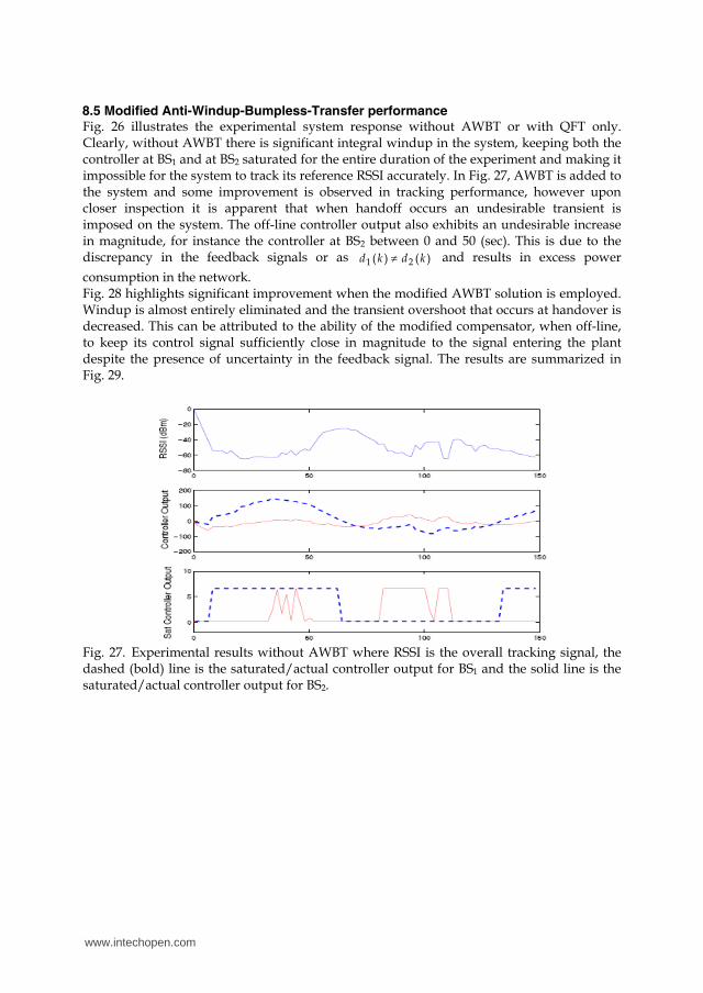
8.5 Modified Anti-Windup-Bumpless-Transfer performance Fig. 26 illustrates the experimental system response without AWBT or with QFT only. Clearly, without AWBT there is significant integral windup in the system, keeping both the controller at BS1 and at BS2 saturated for the entire duration of the experiment and making it impossible for the system to track its reference RSSI accurately. In Fig. 27, AWBT is added to the system and some improvement is observed in tracking performance, however upon closer inspection it is apparent that when handoff occurs an undesirable transient is imposed on the system. The off-line controller output also exhibits an undesirable increase in magnitude, for instance the controller at BS2 between 0 and 50 (sec). This is due to the discrepancy in the feedback signals or as )()( 21 kdkd and results in excess power consumption in the network. Fig. 28 highlights significant improvement when the modified AWBT solution is employed. Windup is almost entirely eliminated and the transient overshoot that occurs at handover is decreased. This can be attributed to the ability of the modified compensator, when off-line, to keep its control signal sufficiently close in magnitude to the signal entering the plant despite the presence of uncertainty in the feedback signal. The results are summarized in Fig. 29.

Fig. 27. Experimental results without AWBT where RSSI is the overall tracking signal, the dashed (bold) line is the saturated/actual controller output for BS1 and the solid line is the saturated/actual controller output for BS2.

Fig. 28. Experimental results where RSSI is the overall tracking signal, the dashed (bold) line is the saturated/actual controller output for BS1 and the solid line is the saturated/actual controller output for BS2. System response with AWBT compensation

Fig. 29. Experimental results where RSSI is the overall tracking signal, the dashed (bold) line is the saturated/actual controller output for BS1 and the solid line is the saturated/actual controller output for BS2. System response with modified AWBT compensation

Fig. 30. Results in terms of the performance criteria. Standard deviation has units dBm. Average power consumption is given in milliwatts.

www.intechopen.com

Addressing Non-linear Hardware Limitations and Extending Network Coverage Area for Power Aware Wireless Sensor Networks 27

8.5 Modified Anti-Windup-Bumpless-Transfer performance Fig. 26 illustrates the experimental system response without AWBT or with QFT only. Clearly, without AWBT there is significant integral windup in the system, keeping both the controller at BS1 and at BS2 saturated for the entire duration of the experiment and making it impossible for the system to track its reference RSSI accurately. In Fig. 27, AWBT is added to the system and some improvement is observed in tracking performance, however upon closer inspection it is apparent that when handoff occurs an undesirable transient is imposed on the system. The off-line controller output also exhibits an undesirable increase in magnitude, for instance the controller at BS2 between 0 and 50 (sec). This is due to the discrepancy in the feedback signals or as )()( 21 kdkd and results in excess power consumption in the network. Fig. 28 highlights significant improvement when the modified AWBT solution is employed. Windup is almost entirely eliminated and the transient overshoot that occurs at handover is decreased. This can be attributed to the ability of the modified compensator, when off-line, to keep its control signal sufficiently close in magnitude to the signal entering the plant despite the presence of uncertainty in the feedback signal. The results are summarized in Fig. 29.

Fig. 27. Experimental results without AWBT where RSSI is the overall tracking signal, the dashed (bold) line is the saturated/actual controller output for BS1 and the solid line is the saturated/actual controller output for BS2.

Fig. 28. Experimental results where RSSI is the overall tracking signal, the dashed (bold) line is the saturated/actual controller output for BS1 and the solid line is the saturated/actual controller output for BS2. System response with AWBT compensation

Fig. 29. Experimental results where RSSI is the overall tracking signal, the dashed (bold) line is the saturated/actual controller output for BS1 and the solid line is the saturated/actual controller output for BS2. System response with modified AWBT compensation

Fig. 30. Results in terms of the performance criteria. Standard deviation has units dBm. Average power consumption is given in milliwatts.

www.intechopen.com

9. Conclusion

This chapter has presented a new strategy for power control in WSNs where operational longevity is an issue. An a priori level of performance is achieved in terms of packet error rate using minimum power where significant quantisation noise exists in the selection of the appropriate transmission power. Robustness to a variety of communication constraints have been illustrated using an AWBT scheme. The new approach provides a methodology for the rigorous assessment of the effect that a general class of static memory-less nonlinearity can have on overall system performance in a wireless power control problem setting. Also presented in this chapter was a novel modified AWBT scheme that enables smooth, power aware handoff. The new technique facilitates floor levels on the flow of information to be maintained in a wireless network that arises quite naturally in an ambulatory setting. Feedback discrepancies, hardware limitations and propagation phenomena that are posed by the use of commercially available wireless communication devices were addressed using new signal processing and robust AW design tools. The technique was validated using a fully scalable 802.15.4 compliant wireless testbed that has been a feature of this work. The new AWBT schemes have exhibited significant performance improvements, particularly in terms of transient behaviour at handoff, when compared with analogous systems operating with simple dynamic control only or when AW methods alone were applied within the testbed.

10. Acknowledgements

This work is supported by Science Foundation Ireland under grant 07/CE/I1147 and by the IRCSET Embark Initiative.

11. References

Alavi S.M.M., Walsh M. J. and Hayes M. J. (2008). Distributed power control technique for 802.15.4 wireless sensor networks, based on quantitative feedback theory. Proc. IET Irish Signals and Systems Conference, Pages 260-267, Galway, Ireland.

Andersin M., Rosberg Z., and Zander J. (1998). Distributed discrete power control in cellular pcs, Wireless Personal Communications, Vol. 3, No. 6.

Bernstein D.S. and Michel A.N. (1995). A chronological bibliography on saturating actuators, International Journal of Robust and Nonlinear Control, Vol. 5, Pages 375-380.

Goldsmith A. (2006). Wireless Communications. Cambridge University Press, 2006. Grandhi S. A., Zander J., and Yates R. (1995). Constrained power control, Wireless Personal

Communications, Vol. 2, No. 3. Gunnarsson F., Gustafsson F. and Blom J. (1999). Pole placement design of power control

algorithms, In Proc. IEEE Vehicular Technology Conference, Houston, TX, USA. Hanus R, Kinnaert M, Henrotte J. (1987) Conditioning technique a general anti-windup and

bumpless transfer method. Automatica, Vol. 23, Pages 729–739. Ho Y., lee C. and Chen B. (2006). Robust Hind Power Control for CDMA Cellular

Communication Systems, IEEE Transactions on Signal Processing, Vol. 54, No. 10, Pages 3947-3956.

Horowitz I. (2001). Survey of quantitative feedback theory (QFT), Int. J. Robust Nonlinear Control, Vol. 11, Pages 887-921.

IEEE 802.15.4 Standard (2006). Wireless lan Medium Access Control (MAC) and Physical layer (PHY) specifications for Low-Rate Wireless Personal Area Networks (LR-WPANs), IEEE Std 802.15.4.

IMS Research (2009). Wireless in industrial systems: Cautious enthusiasm. Industrial Embedded Systems, Winter, 2006, Available: http://www.industrial-embedded.com/columns/Market_Pulse/2006/FallWinter/.

Mobihealthnews. Analyst: Wireless health can’t be homebound. March, 2009, Available: http://mobihealthnews.com/1008/analyst-wireless-health-cant-be-homebound/ [Accessed March 2009].

Otto C., Milenkovi A., Sanders C., and Jovanov E. (2006). System architecture of a wireless body area sensor network for ubiquitous health monitoring. Journal of Mobile Multimedia, Vol. 1, No. 4, Pages 307-326.

Polastre J., Szewczyk R., and Culler D. (2005). Telos: enabling ultra-low power wireless research. Proceedings of the 4th international symposium on Information processing in sensor networks, Los Angeles, California, USA.

Rappaport T.S. (2002). Wireless Communications principles and practice. Prentice Hall, second edition.

Srinivasan K. and Levis P. (2006). RSSI is Under Appreciated, Third Workshop on Embedded Networked Sensors (EmNets)

Turner M., Herrmann G. and Postlethwaite I.. (2007). Incorporating robustness requirements into anti-windup design, IEEE Transactions on Automatic Control, Vol. 52, No. 10, Pages 1842-1855.

Turner M, Postlethwaite I. (2004). A new perspective on static and low-order anti-windup synthesis. International Journal of Control, Vol. 77, Pages 27–44.

Walsh M., Alavi S. M. M. and Hayes M. (2008). On the effect of communication constraints on robust performance for a practical 802.15.4 Wireless Sensor Network Benchmark problem. Proc. 47th IEEE Conference on Decision and Control (CDC08), Pages 447-452, Cancun, Mexico.

Walsh M. J., Alavi S.M.M. and Hayes M. J. Practical assessment of hardware limitations on power aware 802.15.4 wireless sensor networks- an anti- wind up approach. International Journal of Robust and Nonlinear Control (in press 2009).

Weston P. F. and Postlewaite I. (2000). Analysis and design of linear conditioning schemes for systems containing saturating actuators, Automatica, Vol. 36, No. 9.

Zurita Ares B., Fischione C., Speranzon A., and Johansson K. H. (2007). On power control for wireless sensor networks: system model, middleware component and experimental evaluation. European Control Conference, Kos, Greece.

www.intechopen.com

Addressing Non-linear Hardware Limitations and Extending Network Coverage Area for Power Aware Wireless Sensor Networks 29

9. Conclusion

This chapter has presented a new strategy for power control in WSNs where operational longevity is an issue. An a priori level of performance is achieved in terms of packet error rate using minimum power where significant quantisation noise exists in the selection of the appropriate transmission power. Robustness to a variety of communication constraints have been illustrated using an AWBT scheme. The new approach provides a methodology for the rigorous assessment of the effect that a general class of static memory-less nonlinearity can have on overall system performance in a wireless power control problem setting. Also presented in this chapter was a novel modified AWBT scheme that enables smooth, power aware handoff. The new technique facilitates floor levels on the flow of information to be maintained in a wireless network that arises quite naturally in an ambulatory setting. Feedback discrepancies, hardware limitations and propagation phenomena that are posed by the use of commercially available wireless communication devices were addressed using new signal processing and robust AW design tools. The technique was validated using a fully scalable 802.15.4 compliant wireless testbed that has been a feature of this work. The new AWBT schemes have exhibited significant performance improvements, particularly in terms of transient behaviour at handoff, when compared with analogous systems operating with simple dynamic control only or when AW methods alone were applied within the testbed.

10. Acknowledgements

This work is supported by Science Foundation Ireland under grant 07/CE/I1147 and by the IRCSET Embark Initiative.

11. References

Alavi S.M.M., Walsh M. J. and Hayes M. J. (2008). Distributed power control technique for 802.15.4 wireless sensor networks, based on quantitative feedback theory. Proc. IET Irish Signals and Systems Conference, Pages 260-267, Galway, Ireland.

Andersin M., Rosberg Z., and Zander J. (1998). Distributed discrete power control in cellular pcs, Wireless Personal Communications, Vol. 3, No. 6.

Bernstein D.S. and Michel A.N. (1995). A chronological bibliography on saturating actuators, International Journal of Robust and Nonlinear Control, Vol. 5, Pages 375-380.

Goldsmith A. (2006). Wireless Communications. Cambridge University Press, 2006. Grandhi S. A., Zander J., and Yates R. (1995). Constrained power control, Wireless Personal

Communications, Vol. 2, No. 3. Gunnarsson F., Gustafsson F. and Blom J. (1999). Pole placement design of power control

algorithms, In Proc. IEEE Vehicular Technology Conference, Houston, TX, USA. Hanus R, Kinnaert M, Henrotte J. (1987) Conditioning technique a general anti-windup and

bumpless transfer method. Automatica, Vol. 23, Pages 729–739. Ho Y., lee C. and Chen B. (2006). Robust Hind Power Control for CDMA Cellular

Communication Systems, IEEE Transactions on Signal Processing, Vol. 54, No. 10, Pages 3947-3956.

Horowitz I. (2001). Survey of quantitative feedback theory (QFT), Int. J. Robust Nonlinear Control, Vol. 11, Pages 887-921.

IEEE 802.15.4 Standard (2006). Wireless lan Medium Access Control (MAC) and Physical layer (PHY) specifications for Low-Rate Wireless Personal Area Networks (LR-WPANs), IEEE Std 802.15.4.

IMS Research (2009). Wireless in industrial systems: Cautious enthusiasm. Industrial Embedded Systems, Winter, 2006, Available: http://www.industrial-embedded.com/columns/Market_Pulse/2006/FallWinter/.

Mobihealthnews. Analyst: Wireless health can’t be homebound. March, 2009, Available: http://mobihealthnews.com/1008/analyst-wireless-health-cant-be-homebound/ [Accessed March 2009].

Otto C., Milenkovi A., Sanders C., and Jovanov E. (2006). System architecture of a wireless body area sensor network for ubiquitous health monitoring. Journal of Mobile Multimedia, Vol. 1, No. 4, Pages 307-326.

Polastre J., Szewczyk R., and Culler D. (2005). Telos: enabling ultra-low power wireless research. Proceedings of the 4th international symposium on Information processing in sensor networks, Los Angeles, California, USA.

Rappaport T.S. (2002). Wireless Communications principles and practice. Prentice Hall, second edition.

Srinivasan K. and Levis P. (2006). RSSI is Under Appreciated, Third Workshop on Embedded Networked Sensors (EmNets)

Turner M., Herrmann G. and Postlethwaite I.. (2007). Incorporating robustness requirements into anti-windup design, IEEE Transactions on Automatic Control, Vol. 52, No. 10, Pages 1842-1855.

Turner M, Postlethwaite I. (2004). A new perspective on static and low-order anti-windup synthesis. International Journal of Control, Vol. 77, Pages 27–44.

Walsh M., Alavi S. M. M. and Hayes M. (2008). On the effect of communication constraints on robust performance for a practical 802.15.4 Wireless Sensor Network Benchmark problem. Proc. 47th IEEE Conference on Decision and Control (CDC08), Pages 447-452, Cancun, Mexico.

Walsh M. J., Alavi S.M.M. and Hayes M. J. Practical assessment of hardware limitations on power aware 802.15.4 wireless sensor networks- an anti- wind up approach. International Journal of Robust and Nonlinear Control (in press 2009).

Weston P. F. and Postlewaite I. (2000). Analysis and design of linear conditioning schemes for systems containing saturating actuators, Automatica, Vol. 36, No. 9.

Zurita Ares B., Fischione C., Speranzon A., and Johansson K. H. (2007). On power control for wireless sensor networks: system model, middleware component and experimental evaluation. European Control Conference, Kos, Greece.

www.intechopen.com

www.intechopen.com

Wireless Sensor NetworksEdited by

ISBN 978-953-307-325-5Hard cover, 342 pagesPublisher InTechPublished online 29, June, 2011Published in print edition June, 2011

InTech EuropeUniversity Campus STeP Ri Slavka Krautzeka 83/A 51000 Rijeka, Croatia Phone: +385 (51) 770 447 Fax: +385 (51) 686 166www.intechopen.com

InTech ChinaUnit 405, Office Block, Hotel Equatorial Shanghai No.65, Yan An Road (West), Shanghai, 200040, China

Phone: +86-21-62489820 Fax: +86-21-62489821

How to referenceIn order to correctly reference this scholarly work, feel free to copy and paste the following:

Michael Walsh and Martin Hayes (2011). Addressing Non-linear Hardware Limitations and Extending NetworkCoverage Area for Power Aware Wireless Sensor Networks, Wireless Sensor Networks, (Ed.), ISBN: 978-953-307-325-5, InTech, Available from: http://www.intechopen.com/books/wireless-sensor-networks/addressing-non-linear-hardware-limitations-and-extending-network-coverage-area-for-power-aware-wirel