MIC-GPU: Transmission CT: Data Generation High …mueller/research/rapidCT/6_parallelism.pdf · High-Performance Computing for Medical Imaging on Programmable Graphics ... pixel voxel

MIC-GPU: High-Performance Computingfor Medical Imagingon Programmable Graphics

Hardware (GPUs)

Parallelism in Medical Imaging

Stony Brook University

Computer Science

Stony Brook, NY

Klaus Mueller, Ziyi Zheng, Eric Papenhausen

SPIE Medical Imaging 2010SPIE Medical Imaging 2011 MIC-GPU 2

Transmission CT: Data Generation

X-ray source

detector

attenuating object


CT Reconstruction

High-dose CT reconstruction usually uses FDK algorithm

• backprojection of filtered views

Low-dose CT reconstruction pipeline typically uses iterative 3D reconstruction with regularization

• projection of volume into set’s views

• correction factor computation

• backprojection of correction factors (views)

• regularization


Filtered BackprojectionReconstruction

Projection filteringFFT

multiply by ramp inverse FFT

pre-weighting BackprojectionsPost-weighting

X-ray source

detectorattenuating object


Iterative Reconstruction

Projections

Initialization

Correction factor computations

BackprojectionsRegularization

X-ray source

detectorattenuating object


Kernel-Centric Decomposition

IterativeFBP

P

C

B

R

B

P Projection

B Backprojection

C Correction

R Regularizationkernel



We can consider each of these steps to be a SIMT kernel

Iterative 3D reconstruction with regularization:

• backprojection of volume into set’s views projection kernel

• correction factor computation correction factor kernel

• backprojection of correction factors backprojection kernel

• regularization regularization kernel

vector operations

projector with interpolation

image processing filters



IterativeFBP

P

C

B

R

B

P Projection

B Backprojection

C Correction

R Regularizationcompute intensive kernel


Kernel Scheduling

SIMT can only execute one kernel at a time

• this prohibits kernel overlap, even if mathematically correct

• we may merge kernels if targets are identical

this favors load balancing and the reduction of passes

First decompose the reconstruction pipeline into components

• develop an optimized kernel for each component

• overlap (=hide) the loading of data (if needed) with execution of a prior kernel (or within kernel)

• optimize what platform to run the computations (CPU, GPU), but then consider transfer of data


Terminology

We shall discuss all material in terms of 3D reconstruction

• the reduction to 2D slice reconstruction is straightforward

Pixels: the basis elements (point samples) of the projection image (the photon measurements)

Voxels: the basis elements (point samples) of the reconstruction volume (the attenuation densities or the tracer photon emissions)

reconstructed volume

interpolation (nearest neighbor, bilinear)

voxelpixel

projection operator

projection image


1

k

i l il

lij

i ilk k lj j

ij

i

p v w

ww

v vw

λ+

−

= +

Projection (into pixel i)

Normalization

at pixel i

Normalization at voxel j

Backprojection

(into voxel j)

Scanned pixel

New (k+1) and previous (k)

values of voxel j

Iterative CT Example: SART/SIRT

Correction value

SPIE Medical Imaging 2010 MIC-GPU 12


( ) ( )3 11

0 0

: :

MN

i j ij j i ij

j i

P p v w B v p wϕ −−

= =

= ⋅ = ⋅

3

3

1

0

1

0

( )( )

( )

( )

i

i

N

i l il

l

ijNp P

il

l

j j j

ij

p P

p v w

w

S P Vw BP I

v v vw B I

ϕ

ϕ

λ

λ

−

=

−∈

=

∈

− ⋅

− = + = +

SART

S: scanner projections

I: identity projection/volume

_

i set i set

j i ij fdk

p P p P

v p w B S∈ ∈

= = ⋅ FBP


Backprojection: Options

• voxel-driven: sample in projection space

• one write per thread

source


Backprojection: Options

• voxel-driven: sample in projection space

• one write per thread

source source

• pixel-driven, sample in volume space

• multiple writes per thread (scatter)

SPIE Medical Imaging 2010SPIE Medical Imaging 2012

CUDA Memory – Backprojection

MIC-GPU 15

Global Memory Texture Memory

Access Read/Write Read only

Cached No Yes

Subject to coalescing Yes No

Interpolation No support Hardwired

Dimension arbitrary 1D, 2D, 3D (supported

after CUDA 2.0)

volume projections

SPIE Medical Imaging 2010

CUDA Configuration: 2D

thread

block

Y

XZ

MIC-GPU 16


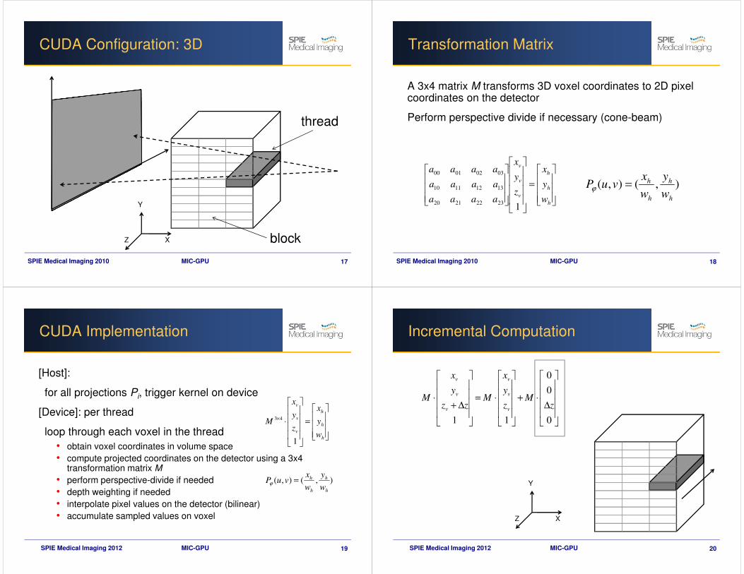
CUDA Configuration: 3D

thread

block

Y

XZ


Transformation Matrix

A 3x4 matrix M transforms 3D voxel coordinates to 2D pixel coordinates on the detector

Perform perspective divide if necessary (cone-beam)

=

h

h

h

v

v

v

w

y

x

z

y

x

aaaa

aaaa

aaaa

123222120

13121110

03020100

),(),(h

h

h

h

w

y

w

xvuP =ϕ


CUDA Implementation

[Host]:

for all projections Pi, trigger kernel on device

[Device]: per thread

loop through each voxel in the thread

• obtain voxel coordinates in volume space

• compute projected coordinates on the detector using a 3x4 transformation matrix M

• perform perspective-divide if needed

• depth weighting if needed

• interpolate pixel values on the detector (bilinear)

• accumulate sampled values on voxel

=

⋅×

h

h

h

v

v

v

w

y

x

z

y

x

M

1

43

),(),(h

h

h

h

w

y

w

xvuP =ϕ


Incremental Computation

MIC-GPU 20

∆⋅+

⋅=

∆+⋅

0

0

0

11

zM

z

y

x

Mzz

y

x

Mv

v

v

v

v

v

Y

XZ


Example: Feldkamp Cone-Beam Reconstruction

360 projections (10242, general position), 5123 volume

CPU

tumor profiles

GPU

performance in seconds

135

80

20

40

60

80

100

120

140

160

CPU GPU


Expressed in Projections/Sec.

360 projections, 5123 volume

Original GPU-recon

performance in projections/s

2.6

45

0

5

10

15

20

25

30

35

40

45

50

CPU GPU


FDK: Medical Datasets

Head Toes Abdominal Aorta

Orig

ina

lR

eco

nstru

cte

d


Forward Projection

Sample in volume space (pixel-driven / ray-driven)

source


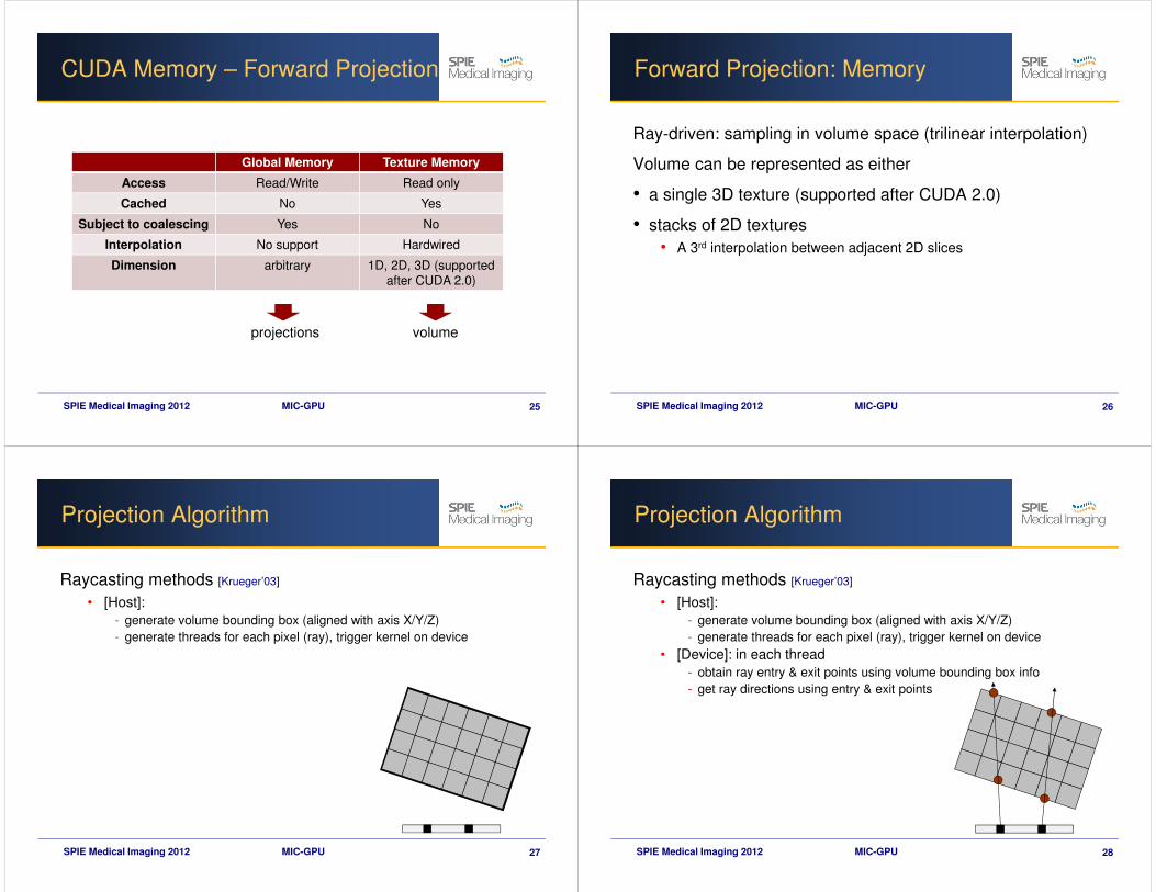
CUDA Memory – Forward Projection

MIC-GPU 25

Global Memory Texture Memory

Access Read/Write Read only

Cached No Yes

Subject to coalescing Yes No

Interpolation No support Hardwired

Dimension arbitrary 1D, 2D, 3D (supported

after CUDA 2.0)

projections volume


Forward Projection: Memory

Ray-driven: sampling in volume space (trilinear interpolation)

Volume can be represented as either

• a single 3D texture (supported after CUDA 2.0)

• stacks of 2D textures

• A 3rd interpolation between adjacent 2D slices

MIC-GPU 26


Projection Algorithm

Raycasting methods [Krueger’03]

• [Host]:

- generate volume bounding box (aligned with axis X/Y/Z)

- generate threads for each pixel (ray), trigger kernel on device




• [Host]:



• [Device]: in each thread

- obtain ray entry & exit points using volume bounding box info

- get ray directions using entry & exit points




• [Host]:



• [Device]: in each thread

- obtain ray entry & exit points using volume bounding box info

- get ray directions using entry & exit points

- cast rays, inside the loop:

• sample in volume space

• accumulate values

• step forward equidistantly


Projection Accuracy

Volume

space

Detector

slice-interpolated grid line Siddon RBF line area Siddon splat

Investigated various schemes in terms of accuracy:

It was shown that the convenient grid-interpolated (trilinear) scheme is qualitatively competitive to the more involved ones listed here.

• see Xu / Mueller, "A comparative study of popular interpolation and integration methods for use in computed tomography," IEEE 2006 International Symposium on Biomedical Imaging (ISBI '06)


Example: Iterative Algorithms

Kernel selection depends on algorithms

Projection/Backprojection

Correction

• pixel-wise operation

• subtraction

Regularization

• TVM or

• bilateral filter or

• non-local mean filter

Sync

Projection

Correction

Backprojection

Regularization

Sync


Sync

MIC-GPU 32

forward projection(pixel-driven)

global memory (r/w) texture memory (r)


Sync

MIC-GPU 33



backprojection(voxel-driven)


Sync

MIC-GPU 34



backprojection(voxel-driven)

add


Regularization

Overall goal: make the reconstruction conform to expectations

• reconstruction is not noisy

• reconstruction has sharp edges

Various techniques

• Total Variation Minimization (TVM)

• bilateral filter (BLF)

• non-local means filter (NLM)

TVM

• motivated by compressive sensing (sparseness) theory

BLF, NLM

• popular in image processing and computer vision

MIC-GPU 35 SPIE Medical Imaging 2010SPIE Medical Imaging 2012

Motivation

Want to remove low-dose CT artifacts:

20 projections SNR=10

CT with low dose data high-dose data CT


Motivation

What we want to achieve – ideally:

20 projections SNR=10

CT + regularization high-dose CT


Total Variation Minimization (TVM)

Goal is to minimize the overall energy:

Minimize using the steepest descent method

• for each voxel vi do iteratively:

MIC-GPU 38

2

0

1| | ( )

2TV

E I I I dxdyλΩ

= ∇ + −

variation fidelity

1 0( )k

k k ki

i i i ik

i

vv v div v v

vβ λ+

∇ = − ⋅ + − ∇

original voxel value


Relaxation Parameters (TVM)

Gradient step size β:

• << 1, usually 0.2

Fidelity term λ:

• initially set to 0

• next iterations:

• assuming:

MIC-GPU 39

02

1( )( )

| | | |

Idiv I I dxdy

Iλ

σ Ω

∇= −

Ω ∇

2 2

0

1min | | subject to ( )

| |I

I dxdy I I dxdy σΩ Ω

∇ − =Ω


Non-linear Neighborhood Filters

40

2 5 6

4 2 7

5 2 6

Input imageWindow

13

Output image

ComputationBased on

Neighborhood values

• Generalization of discrete convolution


Bilateral Filter (BLF)

• Edge-preserving non-linear filter:

41

original edge bilateral filter smoothed edge


Bilateral Filter (BLF)

• Edge-preserving non-linear filter:

42

( ( ) ( )

(

( )( ) )

( )

)(( )) ) (

s f f xc

s f

f d

u

c dx

x

x f

xξξ

ξ ξ

ξ

ξ

ξ∞ ∞

−∞ −∞∞ ∞

−∞ −∞

−

=

−

−

−

spatial closeness value closeness (similarity)


Non-Local Means Filter

Replaces a pixel at x with the mean of the pixels y with similar Gaussian-weighted neighborhood:

(search) window W

Gaussian-weighted neighborhood

patches with pixels y

(only highly-weighted shown)

patch with updated pixel x


Non-Local Means Filter

Replaces a pixel at x with the mean of the pixels y with similar Gaussian-weighted neighborhood:

x, y, t: spatial variables W: window centered at x

N: neighborhood centered at x, y Ga: Gaussian kernel

h: filtering weight controls the influence of dissimilar pixels

2

2

2

2

( ) ( ) ( )

( ) ( ) ( )

( )

( )

at N

at N

G t im g x t im g y t

hy W

G t im g x t im g y t

hy W

e im g y

N LM x

e

∈

∈

+ − +−

∈

+ − +−

∈

=


NLM vs. TVM: Quality

NLM is as good (often better) than TVM

input TVM, =40 NLM, h=15


NLM vs. TVM: Speed

NLM is typically faster than TVM because it is non-iterative

• all parameters were manually set to yield similar visual quality

• CUDA GPU implementations (NVIDIA GTX 480)

• in seconds:

MIC-GPU 46

Image size TV NLM

2562 57 12

5122 80 42


Bilateral vs. NLM

Faster than NLM, but quality is lower

47

NLM

h = 17

rp = 5 rw = 8

Bilateral

x = y = 30

r = 19 rw = 8


Course Schedule

MIC-GPU 48

1:30 – 1:45: Introduction (Klaus)

1:45 – 2:00: Parallel programming primer (Klaus)

2:00 – 2:15: GPU hardware (Ziyi)

2:15 – 3:00: CUDA API, threads (Ziyi)

Coffee Break

3:30 – 4:00: CUDA memory optimization (Eric)

4:00 – 4:15: CUDA programming environment (Ziyi)

4:15 – 4:45: Parallelism in CT reconstruction (Klaus)

4:45 – 5:25: CT reconstruction examples (Eric)

5:25 – 5:30: Closing remarks (Klaus)

Documents

MIC-GPU: Transmission CT: Data Generation High …mueller/research/rapidCT/6_parallelism.pdf · High-Performance Computing for Medical Imaging on Programmable Graphics ... pixel voxel