Backpropagationmgormley/courses/10601-s18/slides/lecture12... · 2.2.2 Backpropagation Thebackpropagationalgorithm (Rumelhartetal., 1986)isageneralmethodforcomputing the gradient

Backpropagation

1

10-601 Introduction to Machine Learning

Matt Gormley

Lecture 12

Feb 23, 2018

Machine Learning Department

School of Computer Science

Carnegie Mellon University

Neural Networks Outline

• Logistic Regression (Recap)– Data, Model, Learning, Prediction

• Neural Networks– A Recipe for Machine Learning

– Visual Notation for Neural Networks

– Example: Logistic Regression Output Surface

– 2-Layer Neural Network

– 3-Layer Neural Network

• Neural Net Architectures– Objective Functions

– Activation Functions

• Backpropagation– Basic Chain Rule (of calculus)

– Chain Rule for Arbitrary Computation Graph

– Backpropagation Algorithm

– Module-based Automatic Differentiation

(Autodiff)

2

This Lecture

Last Lecture

ARCHITECTURES

3

Neural Network Architectures

Even for a basic Neural Network, there are

many design decisions to make:

1. # of hidden layers (depth)

2. # of units per hidden layer (width)

3. Type of activation function (nonlinearity)

4. Form of objective function

4

Building a Neural Net

5

…

Output

Features

Q: How many hidden units, D, should we use?


6

…

…

Output

Input

Hidden Layer

D = M

1 1 1



7

…

…

Output

Input

Hidden Layer

D = M



8

…

…

Output

Input

Hidden Layer

D = M



9

…

…

Output

Input

Hidden Layer

D < M

What method(s) is

this setting similar to?



10

…

…

Output

Input

Hidden Layer

D > M

What method(s) is

this setting similar to?


Deeper Networks

11

Decision

Functions

…

…

Output

Input

Hidden Layer 1

Q: How many layers should we use?

Deeper Networks

12

Decision

Functions

…

…Input

Hidden Layer 1

…

Output

Hidden Layer 2



Deeper Networks

13

Decision

Functions

…

…Input

Hidden Layer 1

…Hidden Layer 2

…

Output

Hidden Layer 3

Deeper Networks

14

Decision

Functions

…

…

Output

Input

Hidden Layer 1

Q: How many layers should we use?• Theoretical answer:

– A neural network with 1 hidden layer is a universal function approximator

– Cybenko (1989): For any continuous function g(x), there

exists a 1-hidden-layer neural net hθ(x)

s.t. | hθ(x) – g(x) | < ϵ for all x, assuming sigmoid activation

functions

• Empirical answer:– Before 2006: “Deep networks (e.g. 3 or more hidden layers)

are too hard to train”

– After 2006: “Deep networks are easier to train than shallow

networks (e.g. 2 or fewer layers) for many problems”

Big caveat: You need to know and use the right tricks.

Different Levels of

Abstraction

• We don’t know

the “right”

levels of

abstraction

• So let the model

figure it out!

18

Decision

Functions

Example from Honglak Lee (NIPS 2010)

Different Levels of

Abstraction

Face Recognition:– Deep Network

can build up

increasingly

higher levels of

abstraction

– Lines, parts,

regions

19

Decision

Functions


Different Levels of

Abstraction

20

Decision

Functions


…

…Input

Hidden Layer 1

…Hidden Layer 2

…

Output

Hidden Layer 3

Activation Functions

21

…

…

Output

Input

Hidden Layer

Neural Network with sigmoid

activation functions

(F) LossJ = 1

2 (y � y�)2

(E) Output (sigmoid)y = 1

1+ (�b)

(D) Output (linear)b =

�Dj=0 �jzj

(C) Hidden (sigmoid)zj = 1

1+ (�aj), �j

(B) Hidden (linear)aj =

�Mi=0 �jixi, �j

(A) InputGiven xi, �i


22

…

…

Output

Input

Hidden Layer

Neural Network with arbitrary

nonlinear activation functions

(F) LossJ = 1

2 (y � y�)2

(E) Output (nonlinear)y = �(b)

(D) Output (linear)b =

�Dj=0 �jzj

(C) Hidden (nonlinear)zj = �(aj), �j





So far, we’ve

assumed that the

activation function

(nonlinearity) is

always the sigmoid

function…

23

Sigmoid / Logistic Function

logistic(u) ≡ 11+ e−u


• A new change: modifying the nonlinearity

– The logistic is not widely used in modern ANNs

Alternate 1:

tanh

Like logistic function but

shifted to range [-1, +1]

Slide from William Cohen

AI Stats 2010

sigmoid

vs.

tanh

depth 4?

Figure from Glorot & Bentio (2010)



– reLU often used in vision tasks

Alternate 2: rectified linear unit

Linear with a cutoff at zero

(Implementation: clip the gradient

when you pass zero)




– reLU often used in vision tasks

Alternate 2: rectified linear unit

Soft version: log(exp(x)+1)

Doesn’t saturate (at one end)

Sparsifies outputs

Helps with vanishing gradient


Objective Functions for NNs

1. Quadratic Loss:

– the same objective as Linear Regression

– i.e. mean squared error

2. Cross-Entropy:

– the same objective as Logistic Regression

– i.e. negative log likelihood

– This requires probabilities, so we add an additional

“softmax” layer at the end of our network

28

Forward Backward

Quadratic J =1

2(y � y�)2

dJ

dy= y � y�

Cross Entropy J = y� (y) + (1 � y�) (1 � y)dJ

dy= y� 1

y+ (1 � y�)

1

y � 1

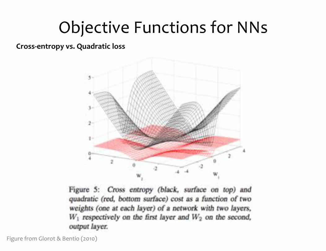
Objective Functions for NNs

Figure from Glorot & Bentio (2010)

Cross-entropy vs. Quadratic loss

Multi-Class Output

30

…

…

Output

Input

Hidden Layer

…

Multi-Class Output

31

…

…

Output

Input

Hidden Layer

…

yk =(bk)

�Kl=1 (bl)

Softmax:(F) LossJ =

�Kk=1 y�

k (yk)

(E) Output (softmax)yk = (bk)�K

l=1 (bl)

(D) Output (linear)bk =

�Dj=0 �kjzj �k

(C) Hidden (nonlinear)zj = �(aj), �j




BACKPROPAGATION

32

A Recipe for

Machine Learning

1. Given training data: 3. Define goal:

33

Background

2. Choose each of these:

– Decision function

– Loss function

4. Train with SGD:

(take small steps

opposite the gradient)

Approaches to

Differentiation

• Question 1:When can we compute the gradients of the

parameters of an arbitrary neural network?

• Question 2:When can we make the gradient

computation efficient?

34

Training

Approaches to

Differentiation

1. Finite Difference Method

– Pro: Great for testing implementations of backpropagation

– Con: Slow for high dimensional inputs / outputs

– Required: Ability to call the function f(x) on any input x2. Symbolic Differentiation

– Note: The method you learned in high-school

– Note: Used by Mathematica / Wolfram Alpha / Maple

– Pro: Yields easily interpretable derivatives

– Con: Leads to exponential computation time if not carefully implemented

– Required: Mathematical expression that defines f(x)

3. Automatic Differentiation - Reverse Mode

– Note: Called Backpropagation when applied to Neural Nets

– Pro: Computes partial derivatives of one output f(x)iwith respect to all inputs x

jin time proportional

to computation of f(x)

– Con: Slow for high dimensional outputs (e.g. vector-valued functions)

– Required: Algorithm for computing f(x)

4. Automatic Differentiation - Forward Mode

– Note: Easy to implement. Uses dual numbers.

– Pro: Computes partial derivatives of all outputs f(x)iwith respect to one input x

jin time proportional

to computation of f(x)

– Con: Slow for high dimensional inputs (e.g. vector-valued x)

– Required: Algorithm for computing f(x)

35

Training

Finite Difference Method

Notes:• Suffers from issues of

floating point precision, in

practice

• Typically only appropriate

to use on small examples

with an appropriately

chosen epsilon

36

Training

Symbolic Differentiation

37

Training

Chain Rule Quiz #1:Suppose x = 2 and z = 3, what are dy/dx

and dy/dz for the function below?

Symbolic Differentiation

Calculus Quiz #2:

39

Training

…

…

…

Chain Rule

Whiteboard– Chain Rule of Calculus

40

Training

Chain Rule

41

Training

2.2. NEURAL NETWORKS AND BACKPROPAGATION

x to J , but also a manner of carrying out that computation in terms of the intermediatequantities a, z, b, y. Which intermediate quantities to use is a design decision. In thisway, the arithmetic circuit diagram of Figure 2.1 is differentiated from the standard neuralnetwork diagram in two ways. A standard diagram for a neural network does not show thischoice of intermediate quantities nor the form of the computations.

The topologies presented in this section are very simple. However, we will later (Chap-ter 5) how an entire algorithm can define an arithmetic circuit.

2.2.2 BackpropagationThe backpropagation algorithm (Rumelhart et al., 1986) is a general method for computingthe gradient of a neural network. Here we generalize the concept of a neural network toinclude any arithmetic circuit. Applying the backpropagation algorithm on these circuitsamounts to repeated application of the chain rule. This general algorithm goes under manyother names: automatic differentiation (AD) in the reverse mode (Griewank and Corliss,1991), analytic differentiation, module-based AD, autodiff, etc. Below we define a forwardpass, which computes the output bottom-up, and a backward pass, which computes thederivatives of all intermediate quantities top-down.

Chain Rule At the core of the backpropagation algorithm is the chain rule. The chainrule allows us to differentiate a function f defined as the composition of two functions gand h such that f = (g �h). If the inputs and outputs of g and h are vector-valued variablesthen f is as well: h : RK

! RJ and g : RJ! RI

) f : RK! RI . Given an input

vector x = {x1

, x2

, . . . , xK}, we compute the output y = {y1

, y2

, . . . , yI}, in terms of anintermediate vector u = {u

1

, u2

, . . . , uJ}. That is, the computation y = f(x) = g(h(x))can be described in a feed-forward manner: y = g(u) and u = h(x). Then the chain rulemust sum over all the intermediate quantities.

dyi

dxk=

JX

j=1

dyi

duj

duj

dxk, 8i, k (2.3)

If the inputs and outputs of f , g, and h are all scalars, then we obtain the familiar formof the chain rule:

dy

dx=

dy

du

du

dx(2.4)

Binary Logistic Regression Binary logistic regression can be interpreted as a arithmeticcircuit. To compute the derivative of some loss function (below we use regression) withrespect to the model parameters ✓, we can repeatedly apply the chain rule (i.e. backprop-agation). Note that the output q below is the probability that the output label takes on thevalue 1. y⇤ is the true output label. The forward pass computes the following:

J = y⇤log q + (1 � y⇤

) log(1 � q) (2.5)

where q = P✓

(Yi = 1|x) =

1

1 + exp(�

PDj=0

✓jxj)(2.6)

13






! RJ and g : RJ! RI


vector x = {x1

, x2


, y2


1

, u2


dyi

dxk=

JX

j=1

dyi

duj

duj

dxk, 8i, k (2.3)


dy

dx=

dy

du

du

dx(2.4)


J = y⇤log q + (1 � y⇤

) log(1 � q) (2.5)

where q = P✓

(Yi = 1|x) =

1

1 + exp(�

PDj=0

✓jxj)(2.6)

13

Chain Rule:Given:

…

Chain Rule

42

Training






! RJ and g : RJ! RI


vector x = {x1

, x2


, y2


1

, u2


dyi

dxk=

JX

j=1

dyi

duj

duj

dxk, 8i, k (2.3)


dy

dx=

dy

du

du

dx(2.4)


J = y⇤log q + (1 � y⇤

) log(1 � q) (2.5)

where q = P✓

(Yi = 1|x) =

1

1 + exp(�

PDj=0

✓jxj)(2.6)

13






! RJ and g : RJ! RI


vector x = {x1

, x2


, y2


1

, u2


dyi

dxk=

JX

j=1

dyi

duj

duj

dxk, 8i, k (2.3)


dy

dx=

dy

du

du

dx(2.4)


J = y⇤log q + (1 � y⇤

) log(1 � q) (2.5)

where q = P✓

(Yi = 1|x) =

1

1 + exp(�

PDj=0

✓jxj)(2.6)

13

Chain Rule:Given:

…Backpropagationis just repeated

application of the

chain rule from

Calculus 101.

Documents

Backpropagationmgormley/courses/10601-s18/slides/lecture12... · 2.2.2 Backpropagation Thebackpropagationalgorithm (Rumelhartetal., 1986)isageneralmethodforcomputing the gradient