Embed Size (px)
Citation preview
Methods of targeting observations for the improvement of
weather forecast skill
Thomas H. A. Frame
Departments of Mathematics/Meteorology
University of Reading
December 2006

’Declaration
I confirm that this is my own work and the use of all material from other sources has been properly
and fully acknowledged’
Thomas H. A. Frame
i
Abstract
This thesis is a contribution to the subjects of midlatitudeatmospheric dynamics and targeting
observations for the improvement of weather forecasts. Forthe first time the full spectrum of
singular vectors of the Eady model are considered. The importance and implications of the un-
shielding and modal unmasking mechanisms to the computed singular vectors are discussed. The
computed singular vectors are used to analyse the vertical structure of the singular vector tar-
geting function commonly used in observation targeting, ina vertical cross-section. Through
comparison of this vertical cross-section to the dynamics of singular vectors, inferences about the
scale and qualitative behaviour of the perturbations to which particular regions are ’sensitive’ are
made. In the final section of the thesis, a new targeting method is introduced. This new targeting
method utilises a set of evolved singular vectors to approximate the background errors within the
region identified by a set of targeted singular vectors as dynamically connected to the verification
region. The two sets of singular vectors can then be used as a computationally inexpensive means
of predicting the reduction of forecast error variance thatwill be obtained from a given deploy-
ment of observations. This method differs from previous targeting methods as it makes no use of
stationary norms or Kalman filter theory. It allows for both adynamically determined estimate
of the initial condition errors and allows for the operational data assimilation to be taken into ac-
count. Another major difference between the new targeting method and existing methods, is that
it explicitly predicts the reduction in forecast error variance as the difference between the forecast
error variance with and without the targeted observations.This additional feature introduces the
potential for the prediction of instances where adding observations is likely to lead to anincrease
ii

in the forecast error variance in the verification region.
iii

Acknowledgements
First and foremost I would like to thank my supervisors Alan,Nancy and Andrew for their pa-
tience and support throughout the past few years, and for accepting my periodic absences. I would
also like to thank my examiners for their helpful suggestions, and for not bringing my greatest
fears to life. Further thanks go to everyone at the departments of mathematics and meteorology;
in particular the DA and PWC groups for the chance to sound offon various subjects from time
to time.
Special thanks goes to those who’ve shared their living and office space with me in Sherfield,
Durley and 2u07 - too too many of you to name here - thank you! Thanks to my old friends from
Gelligaer - Gareth, Tommy, Warren - who’ve always been able to find room for me - mostly in
the pub.
To my family: Thank you for always being there for me throughout these past 28+ years.
To my beautiful wife Vivienne: Your infectious enthusiasm for life allows me to look at the
simplest of things with a sense of wonder. Thank you for always being able to capture my full
attention, and never knowing, caring, nor asking what a singular vector is.
iv

Contents
1 Introduction 1
1.1 Forecast-Analysis Systems . . . . . . . . . . . . . . . . . . . . . . . .. . . . . 3
1.2 Adaptive Observations . . . . . . . . . . . . . . . . . . . . . . . . . . . .. . . 8
1.2.1 Summary of Adaptive Observations . . . . . . . . . . . . . . . . .. . . 8
1.2.2 The singular vector method for observations targeting . . . . . . . . . . . 10
1.2.3 The ensemble transform Kalman filter method of observation targeting . 19
1.2.4 Variations of the singular vector and Ensemble Transform Kalman filter
observation targeting methods . . . . . . . . . . . . . . . . . . . . . . . 22
1.3 Thesis Summary . . . . . . . . . . . . . . . . . . . . . . . . . . . . . . . . . . 24
2 The Eady model 26
2.1 Introduction . . . . . . . . . . . . . . . . . . . . . . . . . . . . . . . . . . . .. 26
2.2 The Inviscid, Adiabatic, quasi-geostrophic equationsfor incompressible flow on
a Mid-latitudef -plane. . . . . . . . . . . . . . . . . . . . . . . . . . . . . . . . 27
2.3 The Two-dimensional Eady Model . . . . . . . . . . . . . . . . . . . . .. . . . 36
2.4 Dynamical behaviour of solutions to the 2D Eady Equations . . . . . . . . . . . 40
2.4.1 Form of the general solution to the Eady Equations . . . .. . . . . . . . 40
2.4.2 The Normal Modes of the 2D Eady Equations . . . . . . . . . . . .. . . 42
2.4.3 The ’Continuum Modes’ of the Eady Equations . . . . . . . . .. . . . . 45
2.4.4 Potential Vorticity Untilting/Unshielding . . . . . . .. . . . . . . . . . 48
2.4.5 Modal Unmasking . . . . . . . . . . . . . . . . . . . . . . . . . . . . . 51
2.4.6 Neutral Mode Resonance . . . . . . . . . . . . . . . . . . . . . . . . . .52
3 The Singular Vectors of The 2D Eady model 53
v
3.1 Introduction . . . . . . . . . . . . . . . . . . . . . . . . . . . . . . . . . . . .. 53
3.2 Definition and Computation of the Eady Model Singular Vectors . . . . . . . . . 57
3.2.1 Definition of the singular vectors . . . . . . . . . . . . . . . . .. . . . . 57
3.2.2 Computation of the singular vectors . . . . . . . . . . . . . . .. . . . . 60
3.2.3 On the choice of norm . . . . . . . . . . . . . . . . . . . . . . . . . . . 63
3.3 Implications of the dynamical mechanism of the Eady model for singular vectors 65
3.3.1 Comparison of continuous and discrete perturbations. . . . . . . . . . . 65
3.3.2 Plane-Wave untilting . . . . . . . . . . . . . . . . . . . . . . . . . . .. 67
3.3.3 Modal unmasking . . . . . . . . . . . . . . . . . . . . . . . . . . . . . 74
3.3.4 Summary . . . . . . . . . . . . . . . . . . . . . . . . . . . . . . . . . . 79
3.4 The singular vectors of the Eady model . . . . . . . . . . . . . . . .. . . . . . 81
3.4.1 A note on the indexing convention of the singular vectors . . . . . . . . . 81
3.4.2 12h integration . . . . . . . . . . . . . . . . . . . . . . . . . . . . . . . 82
3.4.3 48h Singular Vectors . . . . . . . . . . . . . . . . . . . . . . . . . . . .90
3.5 Summary . . . . . . . . . . . . . . . . . . . . . . . . . . . . . . . . . . . . . . 99
4 Identification of the location of greatest sensitivity using Singular Vectors 101
4.1 Introduction . . . . . . . . . . . . . . . . . . . . . . . . . . . . . . . . . . . .. 101
4.2 Sensitivity based targeting function . . . . . . . . . . . . . . .. . . . . . . . . . 103
4.3 Sensitivity determined using non-locally-projected singular vectors . . . . . . . . 105
4.3.1 12h integration . . . . . . . . . . . . . . . . . . . . . . . . . . . . . . . 105
4.3.2 48h integration . . . . . . . . . . . . . . . . . . . . . . . . . . . . . . . 107
4.4 Sensitivity determined using locally projected singular vectors . . . . . . . . . . 109
4.4.1 Singular value decomposition . . . . . . . . . . . . . . . . . . . .. . . 109
4.4.2 Invariance of the spectral-height phase-plane sensitivity, to zonal locali-
sations . . . . . . . . . . . . . . . . . . . . . . . . . . . . . . . . . . . 112
4.4.3 Introduction of height-zonal correlation by zonal localisation . . . . . . . 113
vi
4.5 Summary . . . . . . . . . . . . . . . . . . . . . . . . . . . . . . . . . . . . . . 116
5 A singular vector targeting method that introduces dynamic estimates of the initialcondition errors 119
5.1 Basic formulation of a targeting method . . . . . . . . . . . . . .. . . . . . . . 121
5.2 Using singular vectors to reduce the rank of the targeting problem . . . . . . . . 124
5.3 Approximation of the data assimilation response . . . . . .. . . . . . . . . . . . 128
5.4 Implementation of the targeting method in the Eady model. . . . . . . . . . . . 135
5.4.1 A simple definition ofGp . . . . . . . . . . . . . . . . . . . . . . . . . 135
5.4.2 Simplification ofGp . . . . . . . . . . . . . . . . . . . . . . . . . . . . 137
5.4.3 Computing the singular vectors . . . . . . . . . . . . . . . . . . .. . . 138
5.4.4 Examination and dynamical interpretation of the optimal observation lo-
cation . . . . . . . . . . . . . . . . . . . . . . . . . . . . . . . . . . . . 139
5.5 Summary . . . . . . . . . . . . . . . . . . . . . . . . . . . . . . . . . . . . . . 143
6 Conclusions 146
A The Numerical Eady Model 152
A.1 Non-Dimensionalisation and Co-Ordinate Change . . . . . .. . . . . . . . . . . 152
A.2 The Discrete Equations and Numerical Model . . . . . . . . . . .. . . . . . . . 153
A.3 The Effect of Courant Number on the Accuracy of Solution .. . . . . . . . . . . 157
B Orthogonality between plane-waves 161
C The relationship between a simple data assimilation system and a local projectionoperator 163
D Mathematical Symbols 167
vii
CHAPTER 1
Introduction
Meteorology is the study of atmospheric phenomena, particularly as a means of forecasting future
weather events. Weather forecasts are produced by evolvingthe estimated current atmospheric
state forward in time using large non-linear numerical models of the physical and dynamical
processes in the atmosphere. The ability to create accuratenumerical forecasts is reliant on both
the accuracy of these models and the accuracy of the initial conditions. The initial conditions
used in weather forecasting are statistically based ’compromises’ between observational data and
a previous forecast, which are generated by a process known as data assimilation. Since Lorenz
(1963) brought chaos theory to the attention of meteorologists, it has been understood that the
non-linear nature of evolutionary process in the atmosphere causes errors (no matter how small)
in initial conditions supplied to the forecast models to eventually grow into large errors in the
forecast. This chaotic behaviour is referred to as sensitivity to initial conditions and is often
summed up with the flippancy “if a butterfly flaps its wings in Brazil a tornado is set off in
Texas”. As a direct result of the work of Lorenz (1963), meteorologists began to speculate about
the existence of a theoretical upper limits to the times-scales over which an accurate forecast
can be made. Since the publication of Lorenz (1963), improvements in numerical models and
observation density have lead to large improvements in forecast accuracy. With the continued
development of numerical forecasting methods and new observation platforms, it is hoped that
there is still room for improvement before any theoretical limit of predictability is reached.
1

Chapter 1 Introduction
Since the mid 1990s, there has been a move to make forecast generation methods more specific
to the atmospheric flow on a particular day and the requirements of the end user. One part of this
move has been the development of methods by which the observation distribution resulting in the
most accurate forecast may beobjectivelydetermined. With the development of new ’movable’
observation platforms, the possibility of day to day variations in the observation network based on
the specific requirements of the forecast may present itself; Emanuel et al. (1995). Observations
obtained in this manner have come to be known as ’targeted’ or’adaptive’ observations; Lorenz
and Emanuel (1998).
Several questions surround the use of an adaptive observation strategy. Most of these questions
are summed up in the words of Thompson (1957):
“What return in increased predictability can be expected from increasing the overall density of
reporting stations, and how does this compare with the corresponding outlay of funds? Where
is the point of rapidly diminishing return per outlay? How should the new stations be located in
effecting the increase of overall station density?”
Thompson (1957), however, was writing about the development of a larger network offixedob-
servations, and so for ’targeted’ observations a further question exists: What methods can be used
to identify the best observation locations on a day to day basis? Attempting to answer these ques-
tions several targeting methods have already been proposedand tested ’in the field’. This thesis
is a further contribution to the answers to two of these questions, namely,
Where should the additional observations be located?
and
What method should be applied to identifying these locations?
2

Chapter 1 Introduction
Answers to a further ’sub-question’,
Why should the observations be placed in these locations?,
are also sought. An outline of the findings of this thesis can be found at the end of this introduc-
tory chapter. Prior to this, we shall give a more detailed explanation of the subject of adaptive
observations. To put the subject of adaptive observations in context, the following section dis-
cusses the properties of a ’generic’ weather forecasting system. The available literature on the
subject of adaptive observations is then discussed in Section 1.2. The final section of this chapter
contains a summary of the main conclusions and chapter contents of the thesis.
1.1 Forecast-Analysis Systems
This section serves as an illustration of the generic properties of weather forecasting systems. It
is not intended to give a full discussion of the specifics of topic but rather to introduce concepts
and terminologies that will be relevant to subsequent discussions. The production of accurate
weather forecasts requires the ability to perform two tasks: Firstly to propagate an estimate of
the current atmospheric state forward in time; Secondly to make accurate estimates of the current
atmospheric state. The first of these tasks is performed using large numerical weather prediction
(NWP) models. The second is performed by combining observations of the current state of the
atmosphere with an estimate of the atmospheric state from a previous forecast.
NWP models are a set of discrete non-linear equations that approximate the physical and dynam-
ical processes in the atmosphere. The integration of a NWP model over a finite time interval
τ from an initial stateχa(0) to a forecast stateχf (τ) can be written as the non-linear operator
3
Chapter 1 Introduction
equation
χf (τ) = M [χa(0), τ ] (1.1)
whereχ is a vector containing the model state variables (pressure,temperature, velocity at differ-
ent grid points for example) andM is a non-linear operator containing the model equations.
The second task required for the successful production of a forecast needs slightly more expla-
nation. Ideally the model would be initialised using a set ofhomogeneously distributed accurate
observations, at least equal in number to the number of variables in the the model state vector
χ. Unfortunately, due to the high dimension of the model stateand the inaccessibility of many
required observation locations, the observations are neither large enough in number nor homo-
geneous enough in their distribution to specify entirely the model state. In order to solve this
problem the observational data are combined with a previousforecast to produce the estimated
current atmospheric state,χa, based on the estimated statistics of the error in both the forecast
and observations. This process is known as data assimilation. The forecast used in the data as-
similation process is known as the background. The estimated state obtained through the data
assimilation process is known as the analysis. The various data assimilation methods in use in
weather forecasting centres derive from the minimisation of the quadratic cost function
J (χ) =1
2
(
χ− χb)T
B−1(
χ− χb)
+1
2(y − H [χ])T R−1 (y − H [χ]) , (1.2)
where the vectorχ is the control vector1, χb is a vector containing the background,y is a vector
containing the observations,H is the forward model (or observation operator) which transforms
1Here we assume the control vector contains the same variables as the model state. In general any variables that
are uniquely related to the model state can be used for the control vector.
4

Chapter 1 Introduction
the model variables to the observed variables,R is matrix containing an estimate of the covariance
between observational errors, andB is a matrix containing an estimate of the covariance between
the errors in the background. From this cost function the analysisχa can be defined as the vector
χ for which J (χ) is minimised. In order to formulate the cost function, certain assumptions
have to be made about the background and observation errors.These assumptions are, that the
observation and background errors are statistically independent, and that individually the assumed
error statistics must lead to non-singular covariance matrices. The assumption of non-singular
covariance matrices essentially implies that all possiblestates must have a reasonable probability
of existing, even if in the current atmospheric flow they are so unlikely that their probability of
existing is very close to zero. A useful property of the cost function is that if the approximation to
the background and observation errors is ’good’ and the forward model can be approximated by
the linear operatorH, the analysis error covariance matrixA is equal to the inverse of the Hessian
(second derivative with respect toχ) of the cost function; i.e.
A ≡
[
∂2J
∂χ2
]−1
=[
B−1 +HTR−1H]−1
. (1.3)
Ideally the covariance matrices in the cost function would depend on the time of observation and
the observations would be used to correct the model state corresponding to the time of obser-
vation. To make the background error covariance time specific one could in theory evolve the
analysis error covariance matrix. In reality however the dimension of the model state vector is
typically greater than106 so that the background error covariance cannot be stored by current
computers, let alone evolved or explicitly inverted. Due tothe limitations in computational power
and concerns that evolving covariance matrices may become singular, many methods of solving
approximate cost functions have been developed. It is not our intention to give a detailed dis-
5

Chapter 1 Introduction
cussion of these methods but some of the more general properties will be highlighted. One such
approximation to the cost function is the (extended) Kalmanfilter. The essential components of
the (extended) Kalman filter are that the covariances are evolved using a linear approximation
to Equation (1.1) and the observations are assimilated sequentially into the background field at
the ’correct’ time. The computational expense required to implement a Kalman Filter for NWP
models is presently too great for the computers used at meteorological centres. 3D-Var and 4D-
Var data assimilation schemes are commonly used operationally in meteorological centres. The
essential components of 3D-Var are: the background error covariance matrix is assumed to be sta-
tionary in time; spatial correlations between errors in thebackground field are typically assumed
to be separable in the vertical and horizontal directions and isotropic in the horizontal direction;
the cost function is minimised (usually approximately) by an iterative algorithm. In 3D-Var the
observations are assimilated into the background at predetermined discrete intervals (analysis cy-
cles) and the time point in the background field evolution at which the observation are assimilated
does not necessarily correspond to the observation time. 4D-Var is an extension to 3D-Var in
which a linear dynamical model is incorporated into the forward model (observation operator), so
that the distribution of the observations in time is taken into account in the assimilation process.
Due to the sensitivity of non-linear models to errors in the initial conditions, there has been a
move by meteorological services in recent years towards ’ensemble forecasting’. In ensemble
forecasting, rather then creating a single forecast, an ensemble of forecasts is created by adding
small perturbationsδχi to the initial condition. The motivation behind ensemble forecasting is to
make a probabilistic forecast rather than a single deterministic forecast. The most likely forecast
6

Chapter 1 Introduction
can then be given by the ensemble mean
χfi (τ) =
Ne∑
i=1
χfi (τ)
Ne
=
Ne∑
i=1
M [χa(0) + δχi, τ ]
Ne
, (1.4)
whereNe is the number of ensemble members. One immediate question that arises from the en-
semble method is what form should the perturbations to the initial conditions take. Two methods
for generating initial perturbations exist. These are the breeding method and the singular vector
method. The singular vector method is motivated by the assumption that the effect of the data
assimilation process is to randomise the initial conditionerrors; Palmer et al. (1998). Since the
initial condition errors are assumed to be random, it is assumed that by perturbing the initial con-
ditions with the perturbations that grow the most over the forecast integration, the most relevant
information about the forecast error is obtained; Palmer etal. (1998). It is the desire to get the
greatest spread in the ensemble that motivates the use of singular vectors to define perturbations
for ensemble forecasting; Molteni et al. (1996). In meteorological applications, singular vectors
are used as estimates of the phase space directions which amplify the most over a finite time
period. Singular vectors will be discussed in more depth in the next section. Like the singular
vector method, the breeding method aims to maximise the spread of the ensemble, but with the
qualification that the growth be sustainable; Toth and Kalnay (1997). In the breeding method a
small perturbation is added to the initial conditions. Bothinitial conditions are evolved with the
non-linear model over one analysis cycle. The resultant fields are then subtracted from each other
to obtain the evolved perturbation. This evolved perturbation is then reduced in amplitude, added
to the new initial conditions and the process is repeated. This continual evolution and amplitude
reduction is designed to replicate the evolutionary behaviour of the errors over multiple analysis
cycles; Toth and Kalnay (1997).
7

Chapter 1 Introduction
1.2 Adaptive Observations
1.2.1 Summary of Adaptive Observations
The question as to the best deployment of observational resources has long been of interest to
meteorologists; e.g. Thompson (1957). In recent years the development of practical methods
for identifying the best locations for additional observations based on the day to day variations
of the atmosphere has become an active area of research. Thissubject area has been referred
to variously as adaptive or targeted observations. One immediate question which arises from
adaptive observations is how to define what is meant by the best location. Generally speaking,
adaptive observations can be motivated by the desire to achieve two different, but interrelated,
goals. The first possible aim of targeting is to obtain the best analysis achievable with the limited
observational resources. Lorenz and Emanuel (1998) and Morss et al. (2001) have proposed
methods which utilise estimates of the initial condition errors from ensemble forecasts to identify
regions where the initial condition errors are large. By targeting observations to areas with large
initial condition errors it is hoped that the maximum improvement in theanalysiscan be obtained.
Whilst maximally reducing the initial condition errormayreduce the subsequent forecast error,
this is not explicitly the aim of the targeting methods proposed by Lorenz and Emanuel (1998)
and Morss et al. (2001). The other possible goal of adaptive observations is that of reducing
forecast error. For the work in this thesis we are concerned only with this second goal; i.e. that
of maximally reducing forecast error. For current targeting techniques the aim of targeting is
usually defined as finding the observations that will maximally improve the forecast within a
geographically localised verification region at a specific verification time.
Several targeting methods which seek to identify the observation locations that maximally reduce
8
Chapter 1 Introduction
forecast error have been proposed. These targeting methodshave been loosely classified into
two types: those which rely on non-linearly evolved ensembles to incorporate information about
small error dynamics, such as Ensemble Transform [Bishop and Toth (1999)] and the ensemble
transform Kalman filter [Bishop et al. (2001)]; and those which rely on linear approximations to
inform the target selection about the error dynamics, such as gradient sensitivity [Bergot et al.
(1999), Pu et al. (1998)], quasi-inverse linear method [Pu et al. (1997)] and singular vector target-
ing methods [Buizza and Montani (1999), Montani (1998)]. Ofthese methods, two in particular
have come to the fore and were used in determining the observation locations during the ’Atlantic
Thorpex Regional Campaign’ (AtREC) field test of targeted observations in 2003. These two
methods are the singular vector method [Buizza and Montani (1999)] and the ensemble transform
Kalman filter method [Bishop et al. (2001)].
Berliner et al. (1999) set out a simplified but ’well posed’ statistical framework for the targeting
problem. This statistical framework may be summarised as follows: Given an estimate of the
atmospheric state at timet0 and the error statistics associated with that estimate, identify the
observations at a later timet1 that will optimise by some measure the expected errors in the
subsequent forecast att2. Berliner et al. (1999) suggest several measures which may be used to
define an optimality criterion. Of these measures, theexpectedforecast error variance is of most
direct relevance to the targeting methods in the current literature. Berliner et al. (1999) refer to
criteria for observation selection that minimise the expected forecast error variance as A-optimal
criteria. We may summarise the essential components of an A-optimal targeting method as: an
estimate of the error statistics att1, an estimate of the effect of observations on those statistics
and an estimate of the evolution of the statistics up tot2. All the targeting methods discussed in
this section (with appropriate assumptions) can be viewed as roughly falling into this description.
9
Chapter 1 Introduction
Additionally, all the targeting methods discussed in this section rely on the assumption that the
evolution of the error statistics is linear. This is equallytrue of methods which make explicit
use of linear operators and those that rely on non-linearly evolved ensembles. The accuracy
of the linear approximation is dependent on the amplitude ofthe perturbation, since for small
perturbations the amplitude of non-linear terms in a seriesexpansion of the dynamical equations
are smaller than the linear terms. However, since atmospheric dynamics leads to perturbation
amplification, it is expected that the accuracy of the linearapproximation deteriorates over time.
The time period over which the linear approximation is validis referred to as ’the linear regime’.
Several investigations into the duration of the linear regime for perturbations with initial amplitude
consistant with the estimated amplitude of initial condition/analysis errors have determined the
maximum duration of the linear regime to be roughly two to three days; see for example Errico
et al. (1993), Rabier and Courtier (1992) and Vukicevic (1991). The validity of this linearity
assumption is questioned by Gilmour et al. (2001).
1.2.2 The singular vector method for observations targeting
The first of the two targeting methods that were used in the AtREC field experiment is the sin-
gular vector method. In simplistic terms the essential components of the singular vector method
can be summarised thus: A small set of perturbations (the singular vectors) that maximise the
amplification of small perturbations to the initial conditions over the finite forecast integration pe-
riod are calculated; the observations are then targeted to regions in which this set of perturbations
weighted by their amplification over the forecast period have large amplitude. The finer details
of this method are somewhat more complex than this simplistic explanation so we shall break it
down into three sections. Firstly we shall describe the mathematical properties and computation
10
Chapter 1 Introduction
of the singular vectors. Secondly we shall describe the implementation of the targeting method
using the singular vectors. Finally we shall identify some assumptions that may be used to link
the method to the generic description of ’A-optimal’ targeting methods.
To compute the singular vectors, it must first be assumed thatthe dynamical behaviour of the per-
turbations (or errors) we are interested in is well approximated by a linearisation of the dynamical
equations about a time varying background state. For targeting applications, this background state
is the portion of the forecast started att0 which lies betweent1 andt2. This linearisation gives
rise to the linear operator
M [χ(t1), t2] =∂M
∂χ[χ(t1), t2] (1.5)
which approximates the evolution of perturbationsδχ(t1) to the stateχ(t1) over the intervalt1
to t2. The evolution of perturbations over this finite time interval is then described by
δχ(t2) = M [χ(t1), t2] δχ(t1) + O(δχ2). (1.6)
The O(δχ2) terms are assumed to be much smaller thanM [χ(t1), t2] δχ(t1) and neglected,
yielding a linear evolution equation. The use of a linear approximation to the non-linear evolution
of perturbations to the state of atmospheric models is usually justified on the grounds that the
amplitude of the perturbations are assumed to be initially small, and the time periods over which
the approximation is applied does not exceed two to three days. HereafterM [χ(t1), t2] will be
donated simply asM .
The singular vectors used in targeting are obtained by computing the singular value decompo-
sition of the matrixK = E1
2
2 T2ME− 1
2
1 (Buizza and Montani (1999)); whereE− 1
2
1 andE1
2
2 are
11
Chapter 1 Introduction
matrices which normalise the initial and final perturbations respectively, andT2 is a local pro-
jection operator. Here we use the subscripts1 and2 to refer to the time at which each operator
is applied; e.g. those applied to the perturbation att1 are subscripted1. The local projection
operator is an operator that sets the amplitude of the perturbation to zero outside the verification
region and is usually defined as a symmetric matrix; e.g. Buizza (1994). Several definitions of
the terms singular value decomposition, singular vector and singular value appear in the meteo-
rological literature. For clarity we shall restrict our definition of these three terms to that given
in linear algebra texts such as Golub and Van Loan (1983) and Strang (1988). The singular value
decomposition (expansion) is defined
K =
rank(K)∑
i=1
σiuivTi ; (1.7)
whereσi, ui andvi are the singular values, left singular vectors and right singular vectors respec-
tively. By convention the singular values are ordered such that
σ1 ≥ σ2 ≥ . . . σrank(K) > 0. (1.8)
The left and right singular vectors satisfy the orthonormality relationships
vTi vj =
1, i = j
0, i 6= j
, (1.9)
uTi uj =
1, i = j
0, i 6= j
, (1.10)
12

Chapter 1 Introduction
and the equations
Kvi = σiui, (1.11)
and
KTui = σivi. (1.12)
Due to the high dimension of the numerical models used in atmospheric modelling, the matrixK
is too large to allow for direct computation of the singular value decomposition. In practice only
a few of the leading right singular vectors are computed via the Lanczos algorithm; Golub and
Van Loan (1983). By the term ’leading’ singular vector we refer to those associated with large
singular values. From the indexing convention given in Equation (1.8) the leadingN singular
vectors are those corresponding toi = 1 to i = N .
The left and right singular vectors are related to model state perturbations att1 andt2 via
δχi(t1) = E− 1
2
1 vi (1.13)
and
T2δχi(t2) = σiE− 1
2
2 ui; (1.14)
where
δχi(t2) = Mδχi(t1). (1.15)
Each right singular vector can be transformed to a corresponding perturbation of the state vari-
13

Chapter 1 Introduction
ables at timet1. Each left singular vector can be transformed to a local perturbation of the state
variables at timet2. This local perturbation is the localisation of the perturbation evolved from
δχi(t1) over the finite time intervalt1 to t2. From the orthogonality relationships given in Equa-
tions (1.9) and (1.10) it is evident thatδχi(t1) andT2δχi(t2) are orthogonal with respect to the
inner products defined by the matricesE1 andE2 respectively; i.e.
δχTi (t1)E1δχi(t1) =
1, i = j
0, i 6= j
, (1.16)
δχTi (t2)T2E2T2δχi(t2) =
1, i = j
0, i 6= j
. (1.17)
The singular value decomposition of the matrixK can therefore be used to define a set of dy-
namical perturbationsδχi(t1) which are orthonormal with respect to the ’E1 inner product’.
These perturbations evolve over the finite time interval to the corresponding evolved perturba-
tionsδχi(t2). These evolved perturbations are orthonormal within the local region defined by the
local projection operatorT2.
A very important aspect of the singular value decompositionis that the singular vectors form a
complete set. This means that any state perturbationδχ may be written as a linear combination
of either the right or left singular vectors. IfK is not full rank then some of these singular vectors
will be associated with zero singular values. The real powerof singular vectors is seen when a
perturbation to the state att1 is written as the linear combination
δχi(t1) =
Ns∑
i=1
γiE− 1
2
1 vi, (1.18)
14

Chapter 1 Introduction
whereγi = vTi E
1
2
1 δχi(t1) is the ’E1’ projection coefficient ofδχi(t1) onto theith singular vector
andNs is the number of elements in the vectorδχ. When the perturbation att1 is written in this
form then the amplitude within the verification region of theevolved perturbation measured in the
norm defined by the ’E2’ inner product is given by
‖T2δχi(t2)‖2E2
= δχTi (t2)T2E2T2δχi(t2) =
Ns∑
i=1
γiσ2i . (1.19)
Furthermore, if the initial condition errors att1 are ’white’ with respect to theE1 inner product
then the expected value ofγi is equal to a constantγ for all i; Palmer et al. (1998). If the
initial condition error is white with respect to theE1 inner product and the approximation of the
error evolution byM is valid then the expected error variance in the verificationregion att2 as
measured in theE2 norm is given by
E[
‖T2δχi(t2)‖2E2
]
=γ
Ns
Ns∑
i=1
σ2i . (1.20)
Due to the high dimension of the numerical models used in meteorological centres exact calcu-
lation of Equation (1.20) is computationally expensive andtime consuming. Since the Lanczos
algorithm allows the computation of the leading singular vectors without the expense of com-
puting all the singular vectors, Equation (1.20) can be approximated using the firstN singular
vectors.
In singular vector targeting the observations are directedtowards regions in which the amplitudes
of the right singular vectors weighted by their singular values are ’large’; e.g. Buizza and Montani
(1999). The idea being that by reducing the errors in regionswhere the singular vector amplitude
is large one reduces the amplitude of the projectionγi of the error at timet1 onto the leading
right singular vectors. From Equation (1.19) it is evident that reducing the magnitude ofγi for the
15

Chapter 1 Introduction
leading right singular vectors will reduce the forecast error. Furthermore if the initial condition
errors att1 are ’white’ with respect to theE1 inner product and theexpectedeffect of placing
observations in region defined by a local projectionT1 is to uniformly reduce the amplitude of the
error in that region it can be shown that the reduction in expected forecast error variance obtained
by observing inT1 is
E[
‖T2δχi(t2)‖2E2
− ‖T2δχi(t2, T1)‖2E2
]
=γ
Ns
Ns∑
i=1
σ2i v
Ti T1vi, (1.21)
whereδχi(t2, T1) is written as a function ofT1 to distinguish it from the forecast without addi-
tional observations. From this expression it is evident that the singular vector method is in some
ways A-optimal. Equation (1.21) will be discussed in more detail in Chapter 4 however it is intro-
duced here to motivate singular vector targeting as an A-optimal targeting method. A significant
difference between the singular vector method and the A-optimal design of Berliner et al. (1999)
is that in the singular vector method the observations are not explicitly taken into account.
Whilst the use of singular vectors in targeting can be motivated as an A-optimal targeting method,
several other interpretations of their use exist. The specific interpretation of the singular vectors
depends on the choice of the matricesE1 andE2; Palmer et al. (1998). We have already noted
that the A-optimal interpretation of singular vector targeting requires that the matrixE1 is chosen
as the covariance matrix of the initial condition errors att1. In theory, the matrixE2 can be chosen
to measure the aspects of the forecast errors that are considered most vital to remove, however in
practice,E2 is almost universally chosen such that the associated innerproduct is a measure of
the total energy (kinetic energy plus potential energy) of the perturbation. IfE1 is chosen to be the
same asE2, then the singular vector calculation yields the perturbations that amplify the most over
the forecast intervalt1 to t2. In this case the use of singular vector targeting can be motivated by
16

Chapter 1 Introduction
the desire to prevent the errors from growing over the forecast interval. Typically for this optimal
amplification motivation bothE1 andE2 are chosen such that their associated inner products
give the total energy of the perturbation. Palmer et al. (1998) test the consistency of the several
potential metrics with estimates of the analysis error covariance metric. The tested metrics are
total energy, streamfunction, kinetic energy and enstrophy. Of the four metrics that Palmer et al.
(1998) test, it is found the total energy is the least inconsistent with the analysis error covariance
metric. The use of total energy to define the metrics at both the start and end of the forecast interval
can therefore be seen as an attempt to both target the growingerrors and to achieve the A-optimal
goal of minimising the expected forecast error variance. However, since the total energy metric
takes neither the observation network nor the atmospheric dynamics prior tot1 into account, it can
be at best weakly related to the analysis error covariance metric. The use of total energy singular
vectors in targeting is therefore more easily justified on the grounds of preventing error growth.
Barkmeijer et al. (1998) demonstrate the computation of singular vectors using the Hessian of the
3D-Var2 cost function to define the metric att1. These ’Hessian singular vectors’ are computed
using the total energy metric att2 and the Hessian metric att1. Since the metrics differ att2 andt1
the Hessian singular vectors cannot be interpreted as optimally growingperturbations. However
since the inverse of the Hessian matrix is in theory equal to the analysis error covariance matrix
the use of Hessian singular vectors for targeting is more consistent with the A-optimal design
outlined by Berliner et al. (1999). However the background error covariance matrix used in
operational data assimilation systems are not (at present)dependent on the day to day variations
of the atmospheric flow. The background error covariance matrices used in 3D-Var and 4D-
Var are modelled to reflect the climatological statistics ofthe analysis errors so that they can be
applicable to multiple forecast analysis cycles. These background error covariance matrices often
2more recently the Hessian of the (incremental) 4D-Var cost function has been used; Leutbecher (2003)
17
Chapter 1 Introduction
contain many simplifications designed to reduce computational expense. The Hessian metric does
however take explicit account of the location and estimatedaccuracy of routine observations.
In summary, singular vector targeting identifies a region inwhich it is determined that observa-
tions are expected to be most beneficial. This type of targeting can be motivated to a certain
extent by the A-optimal design of Berliner et al. (1999) and/or by the desire to prevent error
growth betweent1 andt2. The exact interpretation of the method depends on the specific choices
of the matricesE1 andE2, which define the metrics att1 andt2 respectively. In the case where
E1 andE2 are identical, the computed singular vectors can be interpreted as the perturbations
which amplify the most with respect to the inner product associated withE1 andE2 over the fi-
nite time intervalt1 to t2. In the case of the identicalE1 andE2 therefore targeting with singular
vectors can be thought of as an attempt to prevent the amplification of errors. Preventing errors
from amplifying however is not necessarily consistent withreducing the forecast error since for
example non-amplifying errors which have large amplitude at t1 may have a significant impact
on the forecast error att2. If however the metric att1 is chosen to represent the statistics of the
analysis errors att1 then the singular vector targeting method can be related to the A-optimality
motivation of Berliner et al. (1999). Since the singular vector targeting method does not explicitly
take into account the character and deployment of the adaptive observations it can arguably only
be A-optimal ’in spirit’ rather than in actuality. Singularvector targeting is more easily thought
of as means of identifying ’sensitive regions’; i.e. regions in which small variations in the initial
conditions are likely to lead to large variations in the forecast.
18
Chapter 1 Introduction
1.2.3 The ensemble transform Kalman filter method of observation targeting
The second of the two targeting methods which have were used during the AtREC experiments
is the ensemble transform Kalman filter; Bishop et al. (2001). The ensemble transform Kalman
Filter has its root in the Ensemble transform technique devised by Bishop and Toth (1999). Both
Ensemble transform and ensemble transform Kalman filters fitcomfortably within the A-optimal
framework of Berliner et al. (1999). The essential aim of both these methods is to predict the fore-
cast error variance att2 associated with a particular deployment of observations att1. In ensemble
transformation, the analysis error covariance matrix associated with a particular deployment of
observations att1 is estimated, using linear transformation ensemble forecast initialised att0. The
approximate analysis error covariance matrix is defined
A1 ≈ D1CCTDT
1 (1.22)
where the columns of the matrixD1 are given by the normalised departuresdi(t1) of the ensemble
membersχf att1 from the ensemble mean andC is a linear transformation to be determined. The
normalise departures are defined
di(t1) =χ
fi (t1) − χ
fi (t1)
(Ne − 1)1
2
; (1.23)
whereχfi (t1) is theith ensemble member att1, χf
i (t1) is the ensemble mean att1 andNe is the
number of ensemble members. The method for determiningC will be discussed a little later. We
shall first concentrate on howC is used to estimate the forecast error for a given deploymentof
observations. Once the transformation matrixC associated with a particular observation deploy-
ment has been determined, the resultant forecast/background error covariance matrix att2 is then
19
Chapter 1 Introduction
approximated by
B2 ≈ D2CCTDT
2 (1.24)
whereD2 is the matrix of normalised departuresdi(t2) at t2. The essential assumption in deter-
mining the relationship betweenA1 andB2 is that the forecast errors evolve linearly about the
forecast trajectory defined by the ensemble mean. This linear assumption implies that
B2 = M[
χf (t1), t2
]
A1MT
[
χf (t1), t2
]
(1.25)
and
D2 = M[
χf (t1), t2
]
D1. (1.26)
Combining Equations (1.22), (1.25) and (1.26) one readily obtains Equation (1.24).
In the ensemble transform technique, the transformation matrix C is computed by specifying the
form of A1 associated with a given observational deployment and solving Equation (1.22) for
C. The ensemble transform Kalman filter is an extension to the ensemble transform technique,
in which the matrixA1 is (theoretically) determined by substituting the approximate background
error covariance
B1 ≈ D1DT1 (1.27)
at t1 into the Hessian of the cost function (Equation (1.3)) and inverting. The transformation
matrix, C, associated with this estimated analysis error covariancematrix is then obtainable as
before from Equation (1.22). The actual calculations used in the ensemble transform Kalman
20
Chapter 1 Introduction
filter are significantly more efficient than these described here. For a full discussion on these
calculations, see Bishop et al. (2001).
To implement the ensemble transform Kalman filter for adaptive observations, the method can
be applied to multiple possible deployments of observations and the most favourable deployment
selected. The favourability of the targeted observations is quantified from the ’signal variance’ at
t2
s(t2) = trace
E1
2
2 T2D2(I − C1CT1 )DTT2E
1
2
, (1.28)
whereE2 andT2 are the “inner product defining” and local projection matrices respectively used
in singular vector targeting; Bishop et al. (2001). As with singular vector targeting total energy
is usually used to defineE2. If the assumption of linear error evolution is valid and theapprox-
imated covariance matricesB1, A1 andR are accurate and consistent with the data assimilation
system used in the weather forecasting centre, then the signal variance is equivalent to the ex-
pected reduction in forecast error variance induced by the observations; Bishop et al. (2001).
This equivalency is also reliant on the accuracy with which the forecast model can evolve a given
initial condition. In practice the matricesB1 andA1 are not consistent with those used in opera-
tional data assimilation systems and the ensemble transform Kalman filter has a tendency to over
estimate the effects of observations on the forecast; Majumdar et al. (2001).
Unlike singular vector targeting, the Ensemble Transform Kalman Filter explicitly takes the as-
similation process into account, although this assimilation process does not correspond to the
actuality of operational assimilation systems. Also, the singular vector method makes no attempt
to identify the optimal observational deployment, and onlydefines a region to be observed. It
must be noted however that the Ensemble Transform Kalman Filter is often used only to generate
21

Chapter 1 Introduction
’summary maps’ of the signal variance, which are then used toidentify target regions, and not
specific observation locations; Majumdar et al. (2002). A second difference between the Ensem-
ble Transform Kalman Filter and singular vector targeting is that, for the singular vector method,
the covariance matrix of the initial condition errors is modelled by the flow-independent matrix
E1, whereas for the ensemble transform Kalman filter the initial condition covariance matrix is
modelled by the flow dependent ensemble perturbations.
1.2.4 Variations of the singular vector and Ensemble Transform Kalman filter ob-
servation targeting methods
Several ’variants’ of the singular vector and ensemble transform Kalman filter targeting meth-
ods have been proposed. Leutbecher (2003) applies the methodology of the ensemble transform
Kalman filter to the Hessian singular vectors used in singular vector targeting. This method ar-
guably has several advantages over both singular vector targeting and the ensemble transform
Kalman filter. In the former case the Hessian reduced rank, asthe method of Leutbecher (2003)
has come to be known, has advantages over the ’regular’ singular vector targeting method in that
it explicitly takes the assimilation process into account in determining the target region. The Hes-
sian reduced rank has two advantages over the ensemble transform Kalman filter method. The
first of these two advantages is that the assimilation schemeassumed by the Hessian reduced rank
is consistent with the operational data assimilation scheme; Leutbecher (2003). A second less ob-
vious advantage is that the use of the local projection operator T2 in the singular vector calculation
means that by design the Hessian singular vectors used in theHessian reduced rank contain only
information relevant to the verification region. By contrast the ensemble members used in the
ensemble transform Kalman filter are designed to maximise the amount of information about the
22

Chapter 1 Introduction
’global’ error statistics. It may be inferred therefore that a greater number of ensemble members
than Hessian singular vectors are required to accurately assess the effects of observations on the
forecast error in the verification region. However the ensemble used in the ensemble transform
Kalman filter is available ’for free’ from the ensemble forecast Majumdar et al. (2001) whereas
the computationally expensive targeting Hessian singularvectors are an added expense to the rou-
tine forecasting system. A very significant difference between the ensemble transform Kalman
filter and the Hessian reduced rank is that while the former takes into account the dynamical evo-
lution of the errors betweent0 andt1 the latter does not since the Hessian of the 3D/incremental
4D VAR cost function is not flow dependent. Kim et al. (2004) propose targeting observations
to locations where non-linearly evolved singular vectors have large amplitude. In the method of
Kim et al. (2004) the singular vectors are computed for the interval t0 to t2 and the target lo-
cations specified using the right singular vector non-linearly evolved tot1. Hamill and Snyder
(2002a) consider the use of background error covariance estimates obtained from an ensemble
Kalman filter to specify the location of observations required to optimally improve the analysis at
t1. This method uses the flow dependent background errors to specify the error statistics att1 but
takes into account that these error statistics may not correspond to the error statistics assumed by
the operational data assimilation system. Although, it must be stressed that the method of Hamill
and Snyder (2002a) is designed to improve the analysis att1 and not the forecast att2. Hamill
and Snyder (2002a)do define a method for determining the forecast improvement att2, but this
additional method is only applicable if an ensemble Kalman filter is used operationally.
23
Chapter 1 Introduction
1.3 Thesis Summary
This thesis covers topics in two areas. In the first half of thethesis, the dynamics of singular
vectors in the Eady model are discussed. In the second half ofthe thesis, this discussion is then
extended to adaptive observations. In this thesis the role of dynamically evolved background er-
rors on the efficacy of targeted observations is examined. Inparticular the effect of using evolved
singular vectors to specify the dynamically organised component of the background error is in-
vestigated. In the first half of the thesis the dynamics of singular vectors in the Eady model are
investigated. In the second half the use of singular vectorsin targeting is investigated. Firstly
the effect of singular vector dynamics on the location of targets identified using singular vectors
is investigated, by considering the singular vector targeting function (e.g. Buizza and Montani
(1999)), which is usually a vertical integral, in the height-zonal plane. Following this a new
targeting method, that utilises these evolved singular vectors to approximate the leading eigen-
vectors of the flow dependent background errors, is introduced. The evolved singular vectors are
combined with the singular vectors used in current singularvector targeting schemes (e.g. Buizza
and Montani (1999)) to estimate the reduction in forecast error variance which will be obtained
from a given deployment of observations. Although this targeting method uses a flow dependent
background error covariance model, it does not rely on the assumption that the operational data
assimilation system is a Kalman filter, as is the case of the ensemble transform Kalman filter
(ETKF) method; Bishop and Toth (1999).
The thesis is divided into chapters as follows:
Chapter 2 contains a description of the Eady model used in this thesis.
Chapter 3 contains an analysis of the singular vectors of theEady model.
24

Chapter 1 Introduction
Chapter 4 contains a examination of the sensitivity based singular vector targeting, in the context
of the Eady model singular vectors.
Chapter 5 contains the description of a new singular vector based targeting method, and the anal-
ysis of the method in the context of the Eady model singular vectors.
Chapter 6 contains a summary of the main conclusions of this thesis.
25

CHAPTER 2
The Eady model
2.1 Introduction
This chapter contains a summary of dynamical properties of the two dimensional Eady Equations.
Discrete versions of the two-dimensional Eady equations are used to define the numerical model
used for experiments in this thesis. The present chapter focuses on the properties of the continuous
equations. The properties of the discrete equations are discussed briefly in the next chapter and in
detail in Appendix A.
The purpose of the present chapter is three-fold. Firstly, the physical motivations of the quasi-
geostrophic equations, upon which the Eady Equations are based, are explained in Section 2.2.
The aim of the discussion of the quasi-geostrophic equations is to motivate the Eady model as a
model of the ’dynamic atmosphere’, and set it in the context of a ’more complete’ model of the
atmosphere. The second purpose for the present chapter is todefine the Eady Equations. Section
2.3 contains the formulation of the Eady Equations. The third purpose of the present chapter
is to introduce the properties of the solutions and dynamical growth mechanisms of the Eady
model which will prove relevant to later discussions. Thesesolutions and growth mechanisms are
described in Section 2.4.
26
Chapter 2 The Eady model
2.2 The Inviscid, Adiabatic, quasi-geostrophic equationsfor incom-
pressible flow on a Mid-latitudef -plane.
The quasi-geostrophic equations approximate the dynamicsof synoptic scale (horizontal scales of
∼ 103km) depressions in the mid-latitude region (30 to 70 degrees north/south of the Equator).
It is from these equations that the Eady model is obtained. Inthis section, we will introduce
the quasi-geostrophic equations. The intention here is to highlight the underlying physics and
dynamics that motivate the equations, rather than to give a fully fledged derivation. A more
detailed treatment of this topic can be found in many fluid dynamics texts such as Pedlosky
(1979) or Holton (1992).
We shall define the quasi-geostrophic equations in Cartesian coordinates and neglect the effects
of the curvature of the Earth. Thex coordinate shall point eastwards, they coordinate northwards
and thez coordinate upwards. Due to the assumed orientation we shallrefer to thex, y, andz
coordinates as the zonal, meridional and vertical coordinates respectively. We will usei, j , k to
denote unit vectors in thex, y andz directions respectively. All parameters will be chosen to be
consistent with the Mid-latitudes.
Many assumptions about, and approximations of, the nature of fluid flow in the atmosphere have
to be made, to obtain the Quasi-geostrophic equations. For concision, we shall list some of the
more basic ones here. Firstly, the atmosphere is assumed to obey the ideal gas law
ρ =p
RT(2.1)
whereρ, p andT are the air density, pressure and temperature respectivelyandR is the gas con-
27
Chapter 2 The Eady model
stant. Secondly, the effects of internal and external frictional forces on the atmosphere have been
neglected. Without these viscous effects, deceleration ofthe winds, by the conversion of kinetic
energy associated with air flow, to thermal energy does not occur within the equations. Thirdly,
diabatic effects due to the presence of water vapour in the atmosphere have been neglected. This
third assumption means that the transfer of thermal energy by evaporation and condensation does
not occur within the Quasi-Geostrophic equations. Fourthly, due to the rotation of the Earth all
fluid elements experience a centripetal acceleration pointing towards the axis of rotation. The
effects of this centripetal acceleration are small and are omitted from the equations. Also due to
the fact that the coordinates are defined in a rotating frame of reference all fluid elements expe-
rience an ’apparent’ acceleration known as the Coriolis acceleration. For the Quasi-geostrophic
equations only the vector component of the Coriolis acceleration pointing in the vertical direction
is retained. The horizontal vector components of the Coriolis acceleration are assumed to be neg-
ligible away from the Equator. A further simplification to the Coriolis acceleration can be made
by assuming the magnitude of vector component pointing in the vertical direction has the constant
valuef0 at all latitudes. Assuming a constant Coriolis acceleration is referred to as thef -plane
approximation1. The ’β effect’ accounts for accelerations due to increased (decreased) planetary
vorticity, when moving in a northwards (southwards) direction, and is important in defining the
planetary scale wave (Rossby wave) motion. Making thef -plane approximation removes the
’β effect’ and therefore planetary scale motion is poorly represented in the equations of motion.
Finally, the gravitational acceleration is assumed to takethe constant valueg at all locations.
We have already made several general simplifying assumptions about the properties of atmo-
spheric motion in the Mid-latitudes. A large number of further simplifying assumptions can be
1Thef -plane approximation is an extension to the ’standard’ Quasi-Geostrophic Equations
28

Chapter 2 The Eady model
made based on observations of the weather systems they are designed to describe. As Eady (1949)
puts it, the dynamical equations can be simplified by ’the omission of all those terms which do
not make a major contribution to the particular type and scale of motion envisaged’. For the
quasi-geostrophic equations the type of motions envisagedare mid-latitude depressions. Obser-
vations of these cyclonic disturbances reveal that: they are convectively stable; they have typical
length and heightL =∼ 103km and H =∼ 10km respectively; and they have typical ve-
locities U =∼ 10ms−1. With these properties in mind we shall now demonstrate the further
simplifications that lead to the quasi-geostrophic equations.
Firstly for convectively stable systems we may (in almost all cases) neglect vertical accelerations
and use hydrostatic balance to describe the vertical structure of the atmosphere; Eady (1949).
Hydrostatic balance is a balance between the force due to vertical pressure gradients and the
gravitational force; i.e.
∂p
∂z= −ρg; (2.2)
wherep is the pressure andρ is the density. The mid-latitude cyclones we wish to describe appear
as small time dependent eddies in a largely hydrostatic atmosphere; the thermodynamic state of
the atmosphere can be expressed as a sum of the stationary component depending on height alone
and an eddy component depending on all spatial coordinates and time thus
p(x, y, z, t) = ps(z) + pe(x, y, z, t), (2.3)
ρ(x, y, z, t) = ρs(z) + ρe(x, y, z, t), (2.4)
θ(x, y, z, t) = θs(z) + θe(x, y, z, t), (2.5)
29

Chapter 2 The Eady model
where the subscriptss ande denote the stationary and eddy components respectively andθ is the
potential temperature. The potential temperature is related to the actual temperature by
θ = T
(
p0
p
)R
Cp
(2.6)
whereCp is the specific heat at constant pressure andp0 is a constant reference pressure, com-
monly chosen to be mean sea-level pressure. It is worth noting here that by definition the wind
velocity makes no contribution to the stationary state and is associated solely with the eddy com-
ponents of the atmosphere. With the cancellation of small terms and the approximation of the
stationary state density and potential temperature by meanvalues, we can ’subtract out’ the sta-
tionary state and define the quasi-geostrophic hydrostaticequation
f0∂ψ
∂z= b, (2.7)
where
b = gθe
θ0(2.8)
is a buoyancy parameter, the stream-functionψ = p/f0ρ0 is a scaled pressure perturbation and
ρ0 andθ0 are the mean values of the stationary state density and buoyancy. The quasi-geostrophic
hydrostatic equation, describes the balance of gravitational and vertical pressure gradient forces
for the eddy components of the atmospheric state. Taking mean values of the stationary state den-
sity and potential temperature is justifiable in this equation on the grounds that observations of the
atmosphere indicate that the magnitude of variations in these quantities are small by comparison
to the absolute magnitude.
30

Chapter 2 The Eady model
Whilst deviations in the magnitude of the stationary state density and potential temperature are
dynamically unimportant, the gradient of these deviationsdoesplay an important role in the dy-
namical evolution of the eddy components of the state. It is the nature of the vertical stratification
of the stationary state that defines the restoring force experienced by air masses displaced in the
vertical direction; i.e. prevents the appearance of convective instability by enforcing the condition
that density is a decreasing function of height. For the quasi-geostrophic equations this stability
property is contained in the static stability parameter
N2 =g
θs
∂θs
∂z, (2.9)
which we shall take to have the constant valueN20 .
The observed propagation speed of the mid-latitude cyclones we wish to represent are much
smaller than the speed of sound (∼ 330ms−1). Since we do not require to represent disturbances
which travel close to the speed of sound we may neglect the dynamical effects of density gra-
dients and assume that the atmosphere is incompressible; i.e. the density is constant in space
and time. It should be pointed out here that in the quasi-geostrophic equations the effect of the
vertical stratification of the stationary state density is retained implicitly in the static stability pa-
rameter and the effect of the vertical density gradients in the eddy components of the state are
retained implicitly in the definition of the Quasi-Geostrophic hydrostatic equation. Since mass is
conserved in the atmosphere, incompressibility enforces the condition that the net flow of mass
into a volume must be zero and therefore the wind must be non-divergent. Zero divergence can
be expressed mathematically as
∇h · v +∂w
∂z= 0, (2.10)
31

Chapter 2 The Eady model
wherev = ui + vj is the horizontal wind velocity,w is the magnitude of the vertical wind
velocity and
∇h =∂
∂xi +
∂
∂yj
is the horizontal gradient operator.
In the atmosphere, the acceleration of air masses due to horizontal pressure gradients is balanced
by two accelerations. Firstly, by the Lagrangian acceleration; i.e. the change in wind velocity.
Secondly, by the Coriolis acceleration which occurs due to the use of a rotating frame of reference
in the equations. The flow is said to be in geostrophic balanceif the pressure gradient acceleration
is equal and opposite to the Coriolis acceleration. The horizontal wind can be separated into a
geostrophically balanced component, the geostrophic windvg, and an unbalanced component,
the ageostrophic windvag. The geostrophic wind is purely horizontal and is defined by
vg = k ×∇hψ. (2.11)
The geostrophic wind is non-divergent. Since the total windfield is non-divergent (Equation
(2.10)) the sum of the ageostrophic and vertical wind must also form a non-divergent circulation.
For geostrophically and hydrostatically balanced flows, there exists a thermal wind balance rela-
tionship
∂vg
∂z=
1
f0k ×∇hb, (2.12)
which relates horizontal gradients of potential temperature2, b, to vertical gradients of the
2N.B. the buoyancy parameter is a scaled potential temperature
32

Chapter 2 The Eady model
geostrophic wind. For example a negative meridional gradient of potential temperature induces
a positive vertical variation in the zonal geostrophic wind. As we shall see the flow in the mid-
latitudes is dominated by the geostrophic wind. Due to the large meridional temperature gradient
(warm at the equator, cold at the poles) the flow in mid-latitudes is dominated by a zonal wind
component which increases in magnitude with height.
The Rossby number
Ro =U
f0L(2.13)
gives an estimate of the typical ratio of the magnitude of theLagrangian acceleration to the Cori-
olis acceleration. When the Rossby number is small the flow isclose to geostrophic balance.
For the mid-latitudes the Coriolis parameter has a valuef0 = 10−4s−1. The typical velocity
and length scales of the cyclones we wish to depict areU ∼ 10ms−1 andL ∼ 103km. With
these valuesRo ∼ 0.1 and the flow is nearly in geostrophic balance and the geostrophic wind
dominates. Since the flow is dominated by the geostrophic wind we can ignore advection of the
eddy components of the state by the ageostrophic and vertical winds; therefore the application of
the Lagrangian time derivative to the eddy components of thestate can be approximated by the
geostrophic Lagrangian time derivative
Dg =∂
∂t+ vg · ∇h. (2.14)
For adiabatic motion, the internal energy of the system remains constant, and entropy is con-
served. For the atmosphere, this is equivalent to assuming that potential temperature is conserved
following the flow. Using the approximation of the Lagrangian time derivative by the quasi-
33

Chapter 2 The Eady model
geostrophic Lagrangian time derivative, potential energyis only approximately conserved. This
approximate conservation is enforced by the thermodynamicequation
Dgb+N20w = 0. (2.15)
The second term (N20w) of this conservation law stems from the advection of the stationary state
potential temperature by the vertical wind. It is assumed that the magnitude of this vertical ad-
vection is too small to significantly alter the properties ofthe stationary state.
On anf − plane the quasi-geostrophic horizontal momentum Equation is defined
Dgvg + f0k × vag = 0. (2.16)
Several terms have been neglected in this equation, most notably the time derivative of the
ageostrophic wind. The ’neglect’ of these terms is only valid if the Rossby number is small.
Applying ∇h× to the quasi-geostrophic horizontal momentum Equation (2.16) and taking the
vertical derivative of the Thermodynamic Equation (2.15),we can combine these two equations
to form
Dg
(
1
f0∇h × vg +
1
N20
∂b
∂z
)
= −∇ ·(
vag + wk)
. (2.17)
Since the divergence of the combined ageostrophic and vertical wind is zero we may define a
quasi-geostrophic potential vorticity
q = ∇h × vg +f0
N20
∂b
∂z(2.18)
which is conserved following the geostrophic flow. The first term on the right hand side of Equa-
34

Chapter 2 The Eady model
tion (2.18) is the vertical component of the vorticity of thegeostrophic wind. The second term
on the right is the vertical gradient of the potential temperature,b. The conservation of potential
vorticity expresses the fact that positive tendencies of vorticity (i.e. deepening of low pressure
systems) are associated with negative tendencies in potential temperature gradient (i.e. warming
at upper levels and cooling at the surface). For negative tendencies in vorticity the opposite is true
so that the development of high pressure systems is associated with cooling above and heating at
the surface. From a physical point of view this heating and cooling is induced by the transport
of warm air from the surface (for low pressure systems) and cold air from upper levels (for high
pressure systems) via the circulation of combined ageostrophic and vertical winds.
From a mathematical point of view the ageostrophic-vertical circulation plays only a diagnostic
role in the quasi-geostrophic equations and the evolution of the flow is determined by the conser-
vative advection of Quasi-Geostrophic potential vorticity by the geostrophic wind. i.e.
Dgq = 0. (2.19)
The quasi-geostrophic potential vorticity can be written as a Laplacian function of the quasi-
geostrophic stream-function
q = ∇2hψ +
f20
N20
∂2ψ
∂z2. (2.20)
With suitable boundary conditions, the potential vorticity can be inverted to obtain the stream-
function field; Hoskins et al. (1985). Once the stream-function is known, every aspect of the
flow can be determined. The quasi-geostrophic equations therefore comprise a simple prognostic
Equation (2.19) which along with suitable (usually time evolving) boundary conditions and the
Laplacian Equation (2.20) can be used to integrate a chosen initial condition forward in time.
35

Chapter 2 The Eady model
Despite the apparent simplicity of the equations non-linearities associated with the advection of
potential vorticity by the geostrophic wind (which dependson the potential vorticity) have so
far prevented the discovery of an analytical solution. To make the Quasi-Geostrophic Equations
solvable by analysis requires further simplifications. Eady (1949) defined a linearised formulation
of the Quasi-Geostrophic equations which allowed both analytical solutions and the retention of
the essential dynamics of cyclogenesis. In the next sectionwe shall introduce the two dimensional
formulation of Eady’s original equations.
2.3 The Two-dimensional Eady Model
In this section, the formulation of the ’Two-Dimensional Eady Equations’ will be described. The
2D Eady Equations are based on a linearisation of the quasi-geostrophic equations about the
time-invariant background state first proposed by Eady (1949). The background state consists of
constant (in space and time) meridional potential temperature gradient
∂b
∂y= −f0Λ, (2.21)
whereΛ is a constant. The over-bar is used to denote a time-invariant background state variable. It
must be stressed that this time-invariant background stateis connected with the eddy components
of the quasi-geostrophic equations and is not part of the stationary hydrostatic state discussed in
the previous section. This time invariant temperature gradient is an approximation to the sus-
tained differential solar heating which supplies the atmosphere with its thermal energy. Through
the thermal wind balance relationship (Equation (2.12)) a vertically sheared zonally orientated
36
Chapter 2 The Eady model
geostrophic flow
ug = Λz, (2.22)
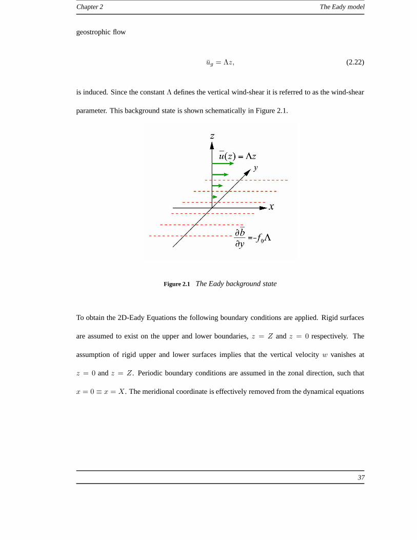
is induced. Since the constantΛ defines the vertical wind-shear it is referred to as the wind-shear
parameter. This background state is shown schematically inFigure 2.1.
Figure 2.1 The Eady background state
To obtain the 2D-Eady Equations the following boundary conditions are applied. Rigid surfaces
are assumed to exist on the upper and lower boundaries,z = Z andz = 0 respectively. The
assumption of rigid upper and lower surfaces implies that the vertical velocityw vanishes at
z = 0 andz = Z. Periodic boundary conditions are assumed in the zonal direction, such that
x = 0 ≡ x = X. The meridional coordinate is effectively removed from thedynamical equations
37

Chapter 2 The Eady model
by assuming that the meridional wavelength of perturbations to the background flow is zero; i.e.
∂ψ′
∂y≡ 0,
x ∈ [0,X]
y ∈ (−∞,∞)
z ∈ (0, Z)
t ∈ [0,∞)
, (2.23)
where the dash denotes a perturbation to the background state. Making this assumption is roughly
equivalent to assuming the zonal scale of perturbations to the background flow is much larger than
the meridional scale and means that solutions to the 2D Eady model are ’technically’ solutions to
the full non-linear Quasi-Geostrophic Equations (Green (1960)). One effect of this assumption
is that flow of wind associated with perturbations to the Eadybackground state exists only in the
meridional direction.
With the above boundary conditions the evolution via Equation (2.19) of potential vorticity per-
turbations to the background flow can be written as
∂
∂t+ Λz
∂
∂x
q′ = 0,
x ∈ [0,X]
y ∈ (−∞,∞)
z ∈ (0, Z)
t ∈ [0,∞)
, (2.24)
where the dash denotes a perturbation perturbation to the Eady background state. The definition
38

Chapter 2 The Eady model
of potential vorticity given in Equation (2.20) becomes
q′ =∂2ψ′
∂x2+f20
N20
∂2ψ′
∂z2
x ∈ [0,X]
y ∈ (−∞,∞)
z ∈ (0, Z)
t ∈ [0,∞)
. (2.25)
Once the potential vorticity can be inverted to obtain the stream-function the model state can be
fully determined.
With the vanishing of vertical velocityw atz = 0 andz = Z the thermodynamic Equation (2.15)
becomes
∂
∂t+ Λz
∂
∂x
∂ψ′
∂z− Λ
∂ψ′
∂x= 0
x ∈ [0,X]
y ∈ (−∞,∞)
z = 0, z = Z
t ∈ [0,∞)
, (2.26)
on the upper and lower boundaries. This new thermodynamic equation defines the evolution of
normal derivative upper and lower boundary conditions required for the inversion of potential
vorticity.
To ensure that the inversion of potential vorticity subjectto periodic and derivative boundary
39

Chapter 2 The Eady model
conditions is unique, a further integral constraint
∫ X
0ψ′dx = 0,
x ∈ [0,X]
y ∈ (−∞,∞)
z ∈ (0, Z)
t ∈ [0,∞)
, (2.27)
is used. This constraint is equivalent to imposing the condition that all non-zero solutions must
be composed of zonal waves.
Equations (2.23) to (2.27) form a complete set which can be used to determine the evolution of
’quasi-two-dimensional’ perturbations to the Eady background state. In all that follows primes
will be dropped from perturbation quantities and all ’un-barred’ variables will be assumed pertur-
bations to the Eady background state. The subscriptg will be dropped from the geostrophic wind,
since the ageostrophic wind makes no explicit appearance inthe Eady Equations. Also since the
solutions to Equations (2.23) to (2.27) are identical at allmeridional locations, the meridional
coordinatey will be removed from the domain of dependence and solutions will be treated as
two-dimensional.
2.4 Dynamical behaviour of solutions to the 2D Eady Equations
2.4.1 Form of the general solution to the Eady Equations
The 2D Eady Equations outlined form an initial boundary value problem to which the solution is
fully determined if the initial stream-function field is known at every point in space. As was noted
in the previous section solutions to the equations are wave-like in the zonal direction. We shall
40

Chapter 2 The Eady model
usekn = 2nπ/X to denote the zonal wavenumber of solutions whereX is the zonal extent of the
domain andn > 0 is an integer which we shall call the wave index. Since at eachtime point the
stream-function field must be a solution to the inversion of potential vorticity the total solution to
the equations comprises a particular (non-zero potential vorticity) solution of the form
ψp(x, z, t) = F (z, t)eiknx (2.28)
whereF is a function of height and time, and a homogeneous (zero potential vorticity) solution
of the form
ψh(x, z, t) = A (t)cosh(knz) + B(t)sinh(knz) eiknx (2.29)
whereA andB are functions of time only.
The original solutions of Eady (1949) consisted of only the zero potential vorticity component of
the solution, which depends only on the potential temperature structure on the upper and lower
boundaries. The zero potential vorticity solutions form a discrete set of normal modes (two for
each wavenumber) the behaviour of which shall be discussed in more detail later. Pedlosky (1964)
noted that the normal modes did not form a full set and therefore the contribution from the ’con-
tinuum of modes’ associated with a non-zero potential vorticity field must be taken into account,
in order to fully describe the behaviour of an arbitrary initial disturbance. A full general solution
to the Eady Equations can be found in Pedlosky (1964), but it is not our intention to give any
formal mathematical discussion of this solution other thannoting its dependence on both normal
modes and ’continuum modes’. In the following sections we shall discuss the structure and be-
haviour of the normal modes; then give a a brief explanation of the structure and behaviour of
the continuum modes; we shall then discuss the behaviour of the untilting plane-wave particular
41

Chapter 2 The Eady model
solution found in Farrell (1984); and finally we will discussthe effect of resonance between the
normal modes and the interior potential vorticity structure.
2.4.2 The Normal Modes of the 2D Eady Equations
The original solutions of Eady (1949) to the Eady Equations contained only the homogeneous
zero potential vorticity component of the solution defined by Equation (2.29). The solutions of
Eady (1949) are of the form
ψh(x, z, t) =
sinh
(
N0
f0knz
)
−N0
f0Λknc cosh
(
N0
f0knz
)
eikn(x−ct) (2.30)
where thecomplexphase speed is given by
c =ZΛ
2±f0Λ
Nkn
√
NZ
2f0kn − coth
(
NZ
2f0kn
)
NZ
2f0kn − tanh
(
NZ
2f0kn
)
. (2.31)
The real component of solutions of this type are the normal modes of the Eady model. Since the
second term of Equation (2.31) can be positive or negative there are two normal modes for each
zonal wavenumber. The vertical structure of the normal modedepends on the zonal wavenumber
but is independent of time. The phase speed of the normal modes is given by the real componentcr
of c and an exponential amplification factor is given byknci whereci is the imaginary component
of c.
The real and imaginary parts of the phase speed (normalised by ΛZ) are shown in Figures 2.2A
and 2.2B respectively. For wavenumbers greater than the critical ’short-wave cutoff’ valuekc =
2.4f0/N0Z, c is entirely real and there are two distinct real phase speedsfor each wavenumber
and the normal modes are non-amplifying. Since their amplitude does not change with time
42
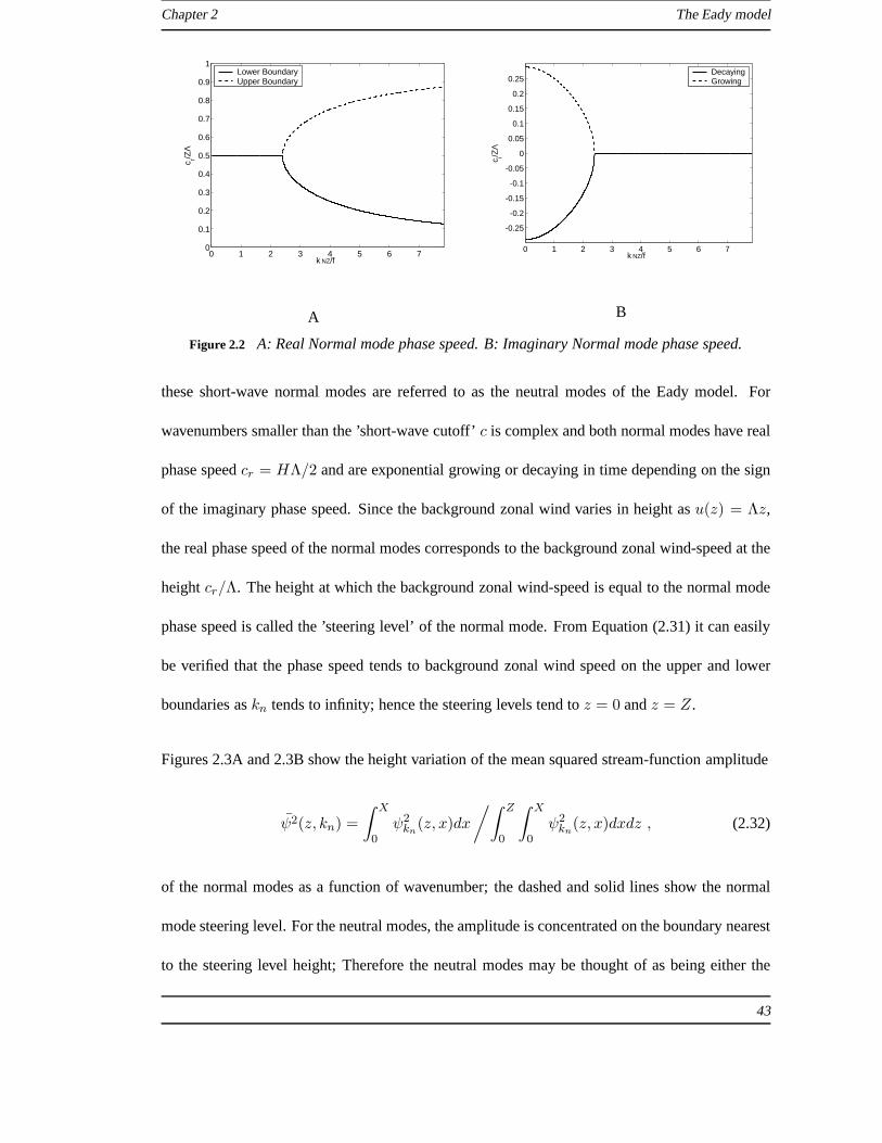
Chapter 2 The Eady model
0 1 2 3 4 5 6 70
0.1
0.2
0.3
0.4
0.5
0.6
0.7
0.8
0.9
1
k NZ/f
c r/ZΛ
Lower BoundaryUpper Boundary
A
0 1 2 3 4 5 6 7
-0.25
-0.2
-0.15
-0.1
-0.05
0
0.05
0.1
0.15
0.2
0.25
k NZ/f
c i/ZΛ
DecayingGrowing
B
Figure 2.2 A: Real Normal mode phase speed. B: Imaginary Normal mode phase speed.
these short-wave normal modes are referred to as the neutralmodes of the Eady model. For
wavenumbers smaller than the ’short-wave cutoff’c is complex and both normal modes have real
phase speedcr = HΛ/2 and are exponential growing or decaying in time depending onthe sign
of the imaginary phase speed. Since the background zonal wind varies in height asu(z) = Λz,
the real phase speed of the normal modes corresponds to the background zonal wind-speed at the
heightcr/Λ. The height at which the background zonal wind-speed is equal to the normal mode
phase speed is called the ’steering level’ of the normal mode. From Equation (2.31) it can easily
be verified that the phase speed tends to background zonal wind speed on the upper and lower
boundaries askn tends to infinity; hence the steering levels tend toz = 0 andz = Z.
Figures 2.3A and 2.3B show the height variation of the mean squared stream-function amplitude
ψ2(z, kn) =
∫ X
0ψ2
kn(z, x)dx
/∫ Z
0
∫ X
0ψ2
kn(z, x)dxdz , (2.32)
of the normal modes as a function of wavenumber; the dashed and solid lines show the normal
mode steering level. For the neutral modes, the amplitude isconcentrated on the boundary nearest
to the steering level height; Therefore the neutral modes may be thought of as being either the
43

Chapter 2 The Eady model
1 2 3 4 5 6 70
0.1
0.2
0.3
0.4
0.5
0.6
0.7
0.8
0.9
1
kNZ/f
z/Z
0.05
0.1
0.15
0.2
0.25
0.3
0.35
0.4
0.45
A
1 2 3 4 5 6 70
0.1
0.2
0.3
0.4
0.5
0.6
0.7
0.8
0.9
1
kNZ/f
z/Z
0.05
0.1
0.15
0.2
0.25
0.3
0.35
0.4
0.45
B
Figure 2.3 Normal mode mean squared amplitude (Equation (2.32)) as a function of height and
zonal wavenumber. A: Decaying mode/lower boundary neutralmode. B: Growing mode/upper
boundary neutral mode. Figures are plotted from verticallydiscretised continuous normal modes.
upper or the lower boundary neutral mode. One noticeable feature of the neutral modes is that the
amplitude resides predominantly between the steering level and the boundary. As the wavenum-
ber increases the steering level moves closer to the boundary and the normal mode amplitude is
contained in an increasingly shallow region at the boundary.
Unlike the neutral modes, the unstable/stable mode’s amplitude is evenly distributed between both
boundaries. Rather than referring to the upper or lower boundary mode, the two components of
the phase speed refer to the growing and decaying modes. For reference examples of the stream-
function structure of the growing (kn = πNZ/2f0), decaying (kn = πNZ/2f0) and lower
boundary neutral (kn = 7πNZ/8f0) modes are shown in Figures 2.4A, 2.4B, 2.4C respectively.
The upper boundary neutral mode is not shown as this is merelya reflection of the lower boundary
neutral mode about the linez = Z/2. The growing neutral modes have a westward phase tilt with
height and the decaying modes have a eastward tilt with height. The magnitude of these phase
tilts decreases with increasing wavenumber.
44

Chapter 2 The Eady model
0 2 4 6 80
0.2
0.4
0.6
0.8
1
xf0/NZ
z/Z
A
0 2 4 6 80
0.2
0.4
0.6
0.8
1
xf0/NZ
z/Z
B
0 2 4 6 80
0.2
0.4
0.6
0.8
1
xf0/NZ
z/Z
C
Figure 2.4 The streamfunction fields associated with A: Growing mode. B: Decaying mode. C:
Neutral mode. The figures are generated by discretising the continuous normal mode.
2.4.3 The ’Continuum Modes’ of the Eady Equations
The normal modes of the Eady model form a discrete set of perturbations associated with the
potential temperature structure on the upper and lower boundaries. Pedlosky (1964) noted that
since there are only two normal modes for each zonal wavenumber, the normal modes do not
form a full set and therefore cannot be used to represent an arbitrary initial disturbance. In order
to be able to represent an arbitrary initial disturbance thecontribution from the potential vorticity
structure in the interior must be taken into account. Using interior potential vorticity perturbations
of the form
q(x, z, t) = Qδ(z − z0)eikn(x−Λz0t), (2.33)
whereQ is a constant wave-amplitude,
δ(z − z0) =
0, z 6= z0,
1, z = z0,
(2.34)
45
Chapter 2 The Eady model
is the Dirac delta function andz0 ∈ (0, Z) is a constant, Pedlosky (1964) solved the 2D Eady
equations in generality. The solution given by Pedlosky (1964) is an unwieldy equation and is not
repeated here; however we shall discuss the some of the qualitative features.
Equation (2.33) defines a zonally orientated potential vorticity travelling wave residing solely at
heightz0. The phase speed of the potential vorticity wave is equal to the background zonal wind
speedu(z0) = λz0 at the heightz0. The stream-function field associated with the potential vor-
ticity wave must satisfy the boundary conditions. For a single potential vorticity wave Pedlosky
(1964) found that he could write the solution as a summation of three separate time dependent
components. The first two of these components are constant multiples of the Eady normal modes
defined by Equations (2.30) and (2.31); where the constant isdefined by the projection of the
initial condition onto the respective normal mode. The third term is the particular solution associ-
ated with the potential vorticity wave. This particular solution comprises a vertically distributed
stream-function field travelling with the phase speed of thepotential vorticity wave. The full so-
lution to the problem is formed from an infinite sum of the potential vorticity wave solutions. The
stream-function fields associated with potential vorticity waves of the form of Equation (2.33)
are collectively known as the continuum modes of the Eady model. The phase of the continuum
modes is constant in height. The phase speed of each continuum mode is equal to the phase speed
of the potential vorticity wave with which it is associated.
A notable feature of the continuum modes is the difference instructure of the low and high
wavenumber modes. To demonstrate this difference Figures 2.5A and 2.5B show the variation
of mean squared stream-function amplitude (Equation (2.32)) with height (y-axis) as a func-
tion of zonal wavenumber (x-axis) for single potential vorticity waves located atz0 = Z/2 and
z0 = 3Z/4 respectively. For reference the dashed and solid black lines show the steering level
46

Chapter 2 The Eady model
height and the dotted black line shows the location of the potential vorticity wave. When the
potential vorticity wave is located in the centre of the domain (Figure 2.5A) the low wavenumber
continuum modes have equal amplitude maxima on the upper andlower boundaries, whereas the
high wavenumber modes have a single amplitude maxima at the location of the potential vorticity
wave. The ’intermediate’ wavenumbers have three maxima onelocated in the centre and one on
each boundary. When the location of the potential vorticitywave is moved toz0 = 3Z/4 (Figure
2.5B) those wavenumbers for which the potential vorticity wave remains sufficiently below the
steering level still have amplitude maxima located at the position of the potential vorticity wave;
whereas those wavenumbers for which the potential vorticity wave is close to or above the upper
boundary steering level have maximum amplitude on the upperboundary.
It is interesting to note that at the high wavenumber end of the zonal spectrum the continuum
modes associated with a potential vorticity wave located near the centre of the domain have neg-
ligible amplitude above (below) the upper (lower) boundarysteering level; whereas the ampli-
tude of normal modes (Figure 2.3) resides almost exclusively above (below) the upper (lower)
boundary steering level. The result of this disparity of structure is that for high wavenumbers the
potential vorticity waves located near the centre of the domain are ’dynamically isolated’ from
the normal modes. By contrast at the low wavenumber end of thezonal spectrum the amplitude
of both the normal modes and the continuum modes is concentrated on the boundaries. This is a
point that we shall return to in our analysis of the singular vector structure of the Eady model.
With the inclusion of the continuum modes in the solution to the 2D Eady Equations there exist
several growth mechanisms additional to the exponential growth associated with the unstable nor-
mal modes. These mechanisms are growth by unshielding/untilting of potential vorticity, growth
by the unmasking of normal modes which are initially masked by continuum modes and growth
47

Chapter 2 The Eady model
1 2 3 4 5 6 70
0.1
0.2
0.3
0.4
0.5
0.6
0.7
0.8
0.9
1
kNZ/f
z/Z
0.05
0.1
0.15
0.2
0.25
0.3
0.35
A
1 2 3 4 5 6 70
0.1
0.2
0.3
0.4
0.5
0.6
0.7
0.8
0.9
1
kNZ/f
z/Z
0.05
0.1
0.15
0.2
0.25
0.3
0.35
0.4
B
Figure 2.5 Continuum mode streamfunction-squared amplitude as a function of height and
wavenumber. A: For a potential vorticity wave residing atz/Z = 0.5. B: For a potential vorticity
wave residing atz/Z = 0.75. Figures are plotted using discretised continuous continuum modes
taken from the solution given in Pedlosky (1964).
by the resonance of the normal modes with the continuum mode located close to the steering level.
Starting with potential vorticity untilting/unshieldingthe properties of these three amplification
mechanisms will be outlined in the subsequent three sections of this chapter.
2.4.4 Potential Vorticity Untilting/Unshielding
Streamfunction amplification via untilting/unshielding relies on the principle of constructive and
destructive superposition of streamfunction waves. For example two superposed streamfunction
waves with the same wavenumber will sum to give a larger amplitude wave if they are in phase.
By contrast the two waves will cancel to give a lower amplitude wave if they are out of phase.
As we have seen in our analysis of the continuum modes of the Eady model, a potential vorticity
wave located at a particular height induces a stream-function field throughout the domain. The
phase speed of this stream-function field is equal to that of the potential vorticity wave. Since
48

Chapter 2 The Eady model
the phase speed of the potential vorticity waves varies withheight, the phase speed of superposed
streamfunction fields associated with potential vorticitywaves on different levels differs. Due
to this difference in phase speed, initially out of phase streamfunction fields can be brought into
phase by the advection of the potential vorticity. As the streamfunction fields are brought into
phase they become increasingly constructively superposed, leading to amplification. This growth
by superposition is encapsulated in the untilting solutionof Farrell (1984).
Farrell (1984) solved the Eady equations for the particularinitial condition3
ψ(x, z, 0) = ei(kx+m0z) = eik(x+a0z), (2.35)
wherek is the zonal wavenumber,m0 is the initial vertical wavenumber anda0 = m/k. The
initial condition given in Equation (2.35) describes uniform amplitude wave-field in which the
phase of the zonal waves is constant along planes which tilt with an angleφ0 = − tan−1 a0 to
the vertical. Since the parametera0 = m/k defines the initial tilt angle of the planes of constant
phase we shall call this theinitial tilt . Following Orr (1907), Farrell (1984) found a particular
solution to the interior potential vorticity equation of the form
ψp(x, z, t) =(1 + a2
0/S)
[1 + (a0 − Λt)2/S]eik(x+[a0−Λt]z) =
(1 + a20/S)
[1 + a2(t)/S]eik(x+a(t)z), (2.36)
whereS = N20 /f
20 anda(t) = a0 − Λt. We shall calla(t) the tilt . For a positive initial tilt the
evolution described by Equation (2.36) may be summarised asfollows: The initial plane wave
structure has a westward tilt with height; over time the tiltreduces due to differential advection
3Since we are dealing with the 2D Eady model the meridional coordinate has been omitted from Farrell (1984)’s
solution.
49
Chapter 2 The Eady model
by the shear flow; along with this reduction in tilt the amplitude increases as per
|ψ| =(1 + a2
0/S)
[1 + (a0 − Λt)2/S]=
(1 + a20/S)
[1 + a2(t)/S]; (2.37)
the amplitude reaches a maximum value of1+a20/S at timet = a0S/Λ; at t = a0S/Λ the planes
of constant phase are parallel to the vertical; beyondt = a0S/Λ the plane waves begin to tilt
eastwards and the amplitude decays with time.
The reason for the amplification of the untilting plane-wavecan be interpreted by considering
the associated potential vorticity field. The particular solution (2.36) is associated with a tilted
potential vorticity plane-wave field of the form
qp(x, z, t) = −k2(1 +a2
0
S)eik(x+a(t)z). (2.38)
This potential vorticity field can be viewed as the infinite sum of potential vorticity waves of
the form Equation (2.33). Each of these potential vorticitywaves induces a vertically distributed
streamfunction field with uniform phase. When the potentialvorticity waves on different levels
are out of phase (i.e. the plane-waves are tilted) the streamfunction fields associated with these
potential vorticity waves are also out of phase leading to destructive superposition. As the po-
tential vorticity waves are brought into phase by the shear-flow the streamfunction function fields
are also brought into phase leading to constructive superposition. On a domain of infinite vertical
extent the amplitude of a streamfunction field associated with a potential vorticity wave would
decay with vertical distance from the potential vorticity ’source’; Bishop and Thorpe (1994). In
this infinite domain case the behaviour of the solution in time could be entirely characterised by
the untilting potential vorticity plane-waves and the local interactions between the streamfunc-
tion fields associated with the potential vorticity structure on adjacent vertical levels. However
50
Chapter 2 The Eady model
the structure of the continuum modes is not in general consistent with that of potential vorticity
waves on an infinite domain and the effect of the upper and lower boundaries on the behaviour of
the solution must be taken into account. In order to satisfy the boundary conditions a contribution
from the homogeneous component of the solution is required.The full solution takes the form
ψ(x, z, t) = ψp(x, z, t) + (A (t)cosh(k/z) + B(t)sinh(kz)) eikx, (2.39)
whereA (t) andB(t) are chosen to satisfy the particular initial condition; Farrell (1984). As we
shall see in the following chapter, the presence of this homogeneous solution plays an important
role in determining the structure of the singular vectors ofthe Eady model. It is worth noting
that unlike the continuum mode solutions of Pedlosky (1964), the behaviour of the homogeneous
component of the plane-wave streamfunction solution is nottrivially related to that of Eady’s
normal mode solutions.
2.4.5 Modal Unmasking
Modal unmasking (Morgan and Chen (2002)) is similar to potential vorticity unshielding in that
it relies on the constructive and destructive superposition of the streamfunction fields associated
with different modes. In modal masking the streamfunction field associated with a normal mode
is ’masked’ by the superposed streamfunction fields associated with the continuum modes. Due
to the difference in phase speed between the continuum modesand normal modes, the normal
mode is ’revealed’. This revealing can be caused either because the net streamfunction field of
the continuum modes decays away due to potential vorticity untilting or because the difference
in phase speed of the normal and continuum modes means that the, initially out of phase, normal
and continuum modes are brought into phase.
51
Chapter 2 The Eady model
2.4.6 Neutral Mode Resonance
Neutral mode resonance is somewhat akin to the exponentially amplifying resonance of the long-
wave normal modes. Neutral mode resonance occurs, however,for wavenumbers greater than
the short-wave cutoff. The essential component of neutral mode resonance is that a potential
vorticity wave resides at the steering level of the neutral normal mode. When this occurs the
interaction between the continuum and normal mode leads to linear amplification of the potential
temperature wave which is sustained indefinitely; Thorncroft and Hoskins (1990). For discrete
numerical models exact neutral mode resonance can only occur if the steering level height for a
particular wavenumber is co-located with one of the models vertical levels and in practice only
approximate resonances are likely; Chang (1992). Unlike the potential vorticity unshielding and
modal unmasking mechanisms, neutral mode resonance (and normal mode resonance) lead to
indefinite growth.
52
CHAPTER 3
The Singular Vectors of The 2D Eady model
3.1 Introduction
The use of singular vector decompositions of linearised dynamical models has become common
in meteorological centres; for example in the generation ofperturbations for ensemble forecasts
Molteni et al. (1996). Singular vectors have come to be associated with the notion of ‘opti-
mal growth’ over finite time intervals; e.g. Buizza et al. (1993). The use of singular vectors to
obtain optimally amplifying perturbations, rather than considering normal modes/eigenvectors,
lies in the fact that since the linear operator associated with small perturbation dynamics in the
atmosphere are not symmetric, their eigenvectors are not orthogonal and therefore a linear com-
bination of eigenvectors may achieve finite time amplification greater than that implied by the
largest eigenvalue; Farrell and Ioannou (1996). The rapid,but transient amplification of singular
vectors has lead them to be associated with rapidly growing forecast errors [e.g. Farrell (1990),
Lorenz (1965)] and the initial stages of rapid cyclogenesis[e.g. Farrell (1989)].
In this chapter the singular vector structure of the 2D Eady model will be described. The work
presented in this chapter follows on from that found in Frameet al. (2005). The singular vectors
of the Eady model with rigid upper and lower boundaries have been presented previously by
Mukougawa and Ikeda (1994), Morgan (2001), Morgan and Chen (2002) and Kim and Morgan
(2002). Several further related studies on the subject of optimal perturbations/singular vectors
53
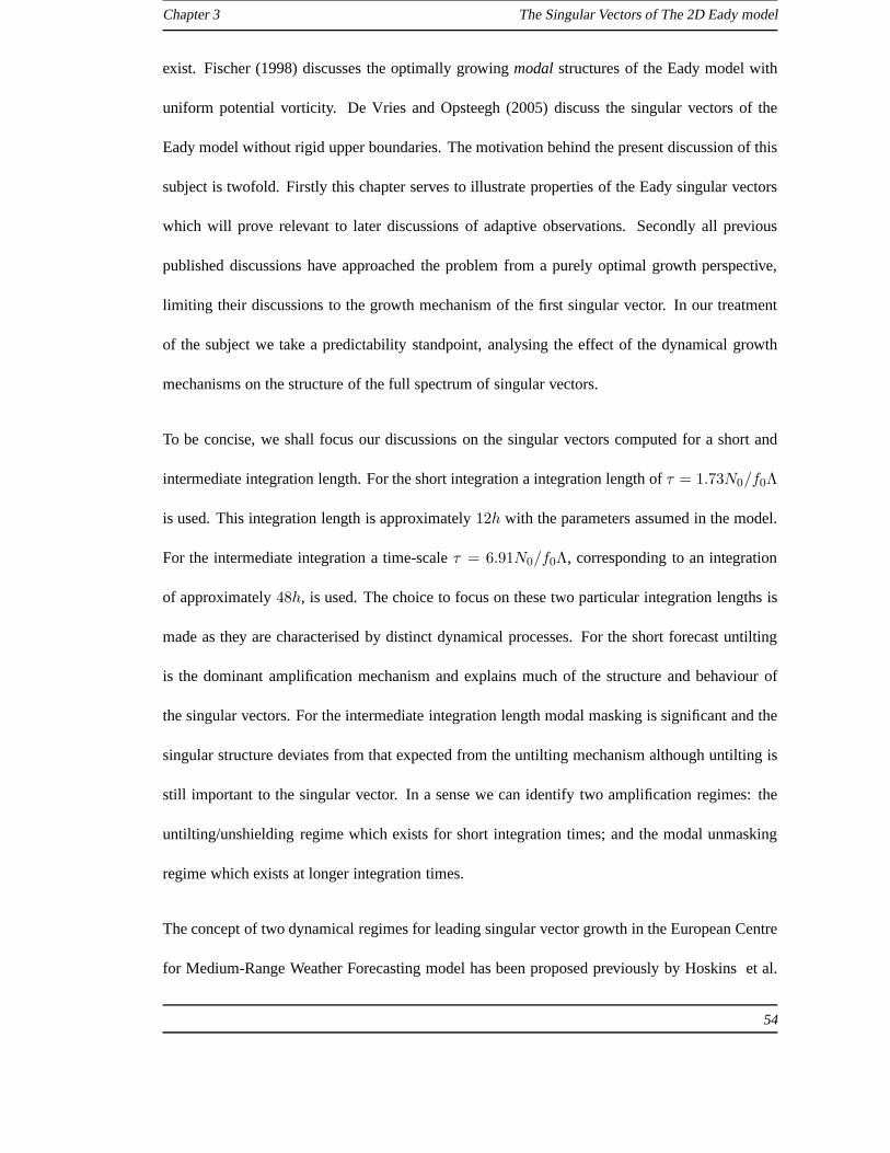
Chapter 3 The Singular Vectors of The 2D Eady model
exist. Fischer (1998) discusses the optimally growingmodalstructures of the Eady model with
uniform potential vorticity. De Vries and Opsteegh (2005) discuss the singular vectors of the
Eady model without rigid upper boundaries. The motivation behind the present discussion of this
subject is twofold. Firstly this chapter serves to illustrate properties of the Eady singular vectors
which will prove relevant to later discussions of adaptive observations. Secondly all previous
published discussions have approached the problem from a purely optimal growth perspective,
limiting their discussions to the growth mechanism of the first singular vector. In our treatment
of the subject we take a predictability standpoint, analysing the effect of the dynamical growth
mechanisms on the structure of the full spectrum of singularvectors.
To be concise, we shall focus our discussions on the singularvectors computed for a short and
intermediate integration length. For the short integration a integration length ofτ = 1.73N0/f0Λ
is used. This integration length is approximately12h with the parameters assumed in the model.
For the intermediate integration a time-scaleτ = 6.91N0/f0Λ, corresponding to an integration
of approximately48h, is used. The choice to focus on these two particular integration lengths is
made as they are characterised by distinct dynamical processes. For the short forecast untilting
is the dominant amplification mechanism and explains much ofthe structure and behaviour of
the singular vectors. For the intermediate integration length modal masking is significant and the
singular structure deviates from that expected from the untilting mechanism although untilting is
still important to the singular vector. In a sense we can identify two amplification regimes: the
untilting/unshielding regime which exists for short integration times; and the modal unmasking
regime which exists at longer integration times.
The concept of two dynamical regimes for leading singular vector growth in the European Centre
for Medium-Range Weather Forecasting model has been proposed previously by Hoskins et al.
54

Chapter 3 The Singular Vectors of The 2D Eady model
(2000). Hoskins et al. (2000) attribute the second regime tolong term normal mode-like growth
due to coupling of potential vorticity with the surface, rather than to transient growth, which can
be interpreted as a modal unmasking effect. Hoskins et al. (2000) propose the transition point
between the two regimes be defined using ‘the two dimensionalquasi-geostrophic expression for
the vertical group velocity of Rossby waves’, with the second regime occuring when the singular
vector energy has propagated to the upper boundary. For the 2D Eady model, in which the merid-
ional potential vorticity gradient is zero, there is no Rossby wave motion and such a definition is
not applicable. In contrast to Hoskins et al. (2000) we find that the transition from the unshield-
ing regime occurs roughly when the integration length is sufficient for a potential vorticity wave
located near the steering level to achieve aπ phase transition relative to the normal mode. As we
shall see, a further implication of this requirement that short wavelength perturbations will enter
the modal unmasking regime at shorter integration lengths than long wavelength perturbations.
Whilst it would be interesting to investigate further the links/contradictions between these two in-
terpretations of the ‘regimes of singular vector growth’, such an investigation will not be included
in this thesis.
The chapter is divided into three sections. In the first section, we outline the singular vector
computation. In the second section we examine the implications of plane-wave untilting and
modal unmasking growth mechanisms for singular vector growth, by considering the properties
of continuous solutions to the Eady model. In the third section, we examine the singular vectors of
the Eady model themselves and seek to relate these to the properties discussed in the first section.
By examining the functional form of the plane-wave solutionof Farrell (1984), several properties
of the untilting mechanism related to singular vectors are identified. Firstly, the optimal initial
tilt for streamfunction amplification over a given finite time interval is identified. It is noted that,
55

Chapter 3 The Singular Vectors of The 2D Eady model
for short time intervals, this optimal tilt is larger than that which would render the plane waves
completely vertical within that time interval. By determining the necessary condition for orthogo-
nality between plane-waves, it is found that the differencein tilt between orthogonal plane waves
is smaller for high wavenumbers than for low wavenumbers. The similarity of the initial tilts of
orthogonal planes at high wavenumbers implies that the finite time amplification of orthogonal
plane waves is more similar at high wavenumbers than low wavenumbers. This means that, when
the amplification of singular vectors other than the first is taken into account, the high wavenum-
bers will be dominant. Although they are not of exact plane-wave form it is found that the12h
singular vectors share the properties of the plane-waves outlined above. It is found that the prop-
erties of the singular vectors are more similar to that of plane-waves at high wavenumbers. This
increased similarity is attributed to the fact that the normal modes have shallower structure at high
wavenumbers and therefore do not ’interfere’ as much in the potential vorticity dynamics at high
wavenumbers.
By extending the concept of an optimal height for modal unmasking of a potential vorticity wave,
that was proposed by De Vries and Opsteegh (2005), the requirement for modal unmasking to lead
to large amplification is inferred. This requirement is thatthe optimal unmasking height coincide
with the region just above (below) the lower (upper) boundary steering level, where the projection
of the continuum modes onto the normal mode is potentially large. Through this connection it
is implied that the transition from the untilting to modal masking regime will occur at shorter
integrations for small zonal scales, than for large zonal scales. Furthermore it is hypothesised that
unlike untilting, modal unmasking cannot characterise thegrowth of large numbers of singular
vectors. This is because modal masking requires the continuum modes to conceal two specific
normal modes, whereas untilting requires that a multiplicity of continuum modes conceal each
56

Chapter 3 The Singular Vectors of The 2D Eady model
other.
3.2 Definition and Computation of the Eady Model Singular Vectors
3.2.1 Definition of the singular vectors
The singular value decomposition was introduced in Chapter1. For convenience we shall re-
iterate the basic points again here. We shall also make definitions of the matrices used in the
singular vector computation which are specific to Eady modelsingular vectors computed in this
thesis. We shall use the matrixL ∈ RNg×Ng to denote an integration of a numerical version of
the Eady model over a finite time intervalτ . The operation of the matrixL is summarised by the
matrix vector equation
ψ(τ) = Lψ(0) (3.1)
whereψ ∈ RNg is vector of grid-point streamfunction values andNg is the number of grid-points.
It is worth noting here that the matrixL will be used only for the Eady model. For discussions of
general linearised dynamical models the matrixM will be used.
As was discussed in the previous chapter, the quasi-geostrophic approximations from which the
Eady model is derived are only applicable to scales of order103km. However for reasons of
numerical accuracy, which will be discussed in the next section, the numerical model resolves
zonal wavelengths much smaller than103km. To filter these smaller zonal wavelengths from the
initial conditions we define a reduced rank discrete Fouriertransform matrixF ∈ R2Nk×Ng . The
matrix F transforms the grid-point streamfunction vectorψ ∈ RNg to the lower dimensional
57

Chapter 3 The Singular Vectors of The 2D Eady model
vector of streamfunction Fourier coefficientsψ ∈ R2Nk , whereNk is the number of resolved
wavelengths greater than a chosen truncation. For the experiments presented in this thesis the
wave-spectrum is truncated at0.8N0Z/f0 which corresponds to800km with the parameters used
in the Eady model. The reverse Fourier transformation is performed by the matrixF T . Since
the rows ofF are orthonormal [Golub and Van Loan (1983)],F T is the pseudo-inverse [Golub
and Van Loan (1983)] ofF . For grid-point streamfunction vectorsψ which do not contain zonal
wavelengths shorter than0.8N0Z/f0, the following relationships are satisfied:
‖ψ‖2 = ‖Fψ‖2, (3.2)
F TFψ = ψ; (3.3)
however these relationships are not satisfied ifψ contains wavelengths smaller than the cutoff
wavelength. For grid-point streamfunction vectors which do contain wavelengths shorter than
0.8N0Z/f0 multiplication by the matrixF TF removes these smaller wavelengths, leaving the
wavelengths longer than0.8N0Z/f0 unchanged. The matrixF TF is a discrete Fourier filter.
The Eady model singular vectors are computed from the matrixLF TF ∈ RNg×Ng . The use of
an initial time Fourier filter is consistent with the singular vector computation methods employed
using more complex models in meteorological centres; e.g. Buizza (1997), LI et al. (2005).
The mathematical properties of the singular vectors are summarised thus. The singular vectors
consist of two complete orthonormal bases. One basis is formed from the right singular vectors
vi ∈ RNg , and the other from the left singular vectorsui ∈ R
Ng . Since they form orthonormal
58

Chapter 3 The Singular Vectors of The 2D Eady model
bases the singular vectors satisfy the relationships
vTi vj =
1, i = j
0, i 6= j
, (3.4)
and
uTi uj =
1, i = j
0, i 6= j
. (3.5)
The left and right singular vectors are linked by the equation
LF TFvi = σiui, i ∈ [1, 2, . . . Ng]. (3.6)
whereσi ∈ R is the corresponding singular value. By convention the singular values and vectors
are ordered such that
σ1 ≥ σ2 ≥ . . . σNg ≥ 0. (3.7)
The right singular vectors can be interpreted as a set of orthogonal initial states. Each of these
initial states evolves over the finite time interval to the corresponding left singular vector mul-
tiplied by the singular value. Since the left singular vectors are orthogonal to each-other, each
of the final states are also orthogonal to each-other. The singular vectors can be viewed as a set
dynamical perturbations for which each perturbation is orthogonal to every other perturbation in
the set at the beginning and at the end of a finite integration.It is this orthogonality property in
combination with the ordering of the singular vectors that guarantees that a linear combination
of singular vectors cannot amplify more than the first singular vector over the integration period
[Farrell and Ioannou (1996)].
59

Chapter 3 The Singular Vectors of The 2D Eady model
An important aspect of singular vectors is that, since they form a complete basis for the model
phase space, there are the same number of singular vectors asthere are degrees of freedom in
the model. It is worth noting here that, due to the presence ofthe Fourier filter matrixF TF ,
degrees of freedom corresponding to zonal wavelengths shorter than0.8N0Z/f0 are associated
with zero singular values. The set of the firstm right singular vectors contains the maximum
information containable inm vectors about the effect of initial random perturbations onthe final
state. Here the term ’random perturbations’ refers to perturbations which are random with respect
to the initial inner product and ’the effect on the final state’ is measured in terms of the norm
deriving from the final inner product. For the Eady model singular vectors computed in this thesis
the 2-norm of the streamfunction field is used as both the initial and final norm. The choice of
norm will be discussed more thoroughly in Section 3.2.3.
3.2.2 Computation of the singular vectors
The singular vectors are computed from the matrixLF TF corresponding to a finite integration
of a numerical version of the Eady model. The details of the discrete equations can be found
in Appendix A but we shall note some of the basic points here. The model is formulated on
a numerical grid withNx = 120 grid points zonally andNz = 51 grid points vertically. The
discrete streamfunction field is defined on all grid-points.The potential vorticity is defined on
all grid-points except the upper-most and lower-most vertical levels. The boundary potential
temperature is defined on the upper-most and lower-most level. The streamfunction is related to
potential vorticity using a5−point approximation to the Laplacian operator and to the upper and
lower boundary potential temperature using a one-sided difference approximation to the vertical
derivative. The use of one-sided approximations to the vertical derivative is motivated by the
60

Chapter 3 The Singular Vectors of The 2D Eady model
fact it allows the numerical model state to be determined by knowledge of the streamfunction
at all grid-points. The zonal derivative is approximated using the ’leapfrog’ scheme. The zonal
advection equations are solved using a centred-time centred-space scheme.
All calculations are performed on a physical domain of dimensionX = 8 × 10³km andZ =
10km corresponding to spatial steps∆x = 66.6km and∆z = 0.2km respectively. A time-
step∆t = 11.0min is used. Parameter valuesf0 = 10−4s−1, N0 = 10−2s−1 andΛ = 4 ×
10−3s−1 are used. For numerical accuracy, the time, zonal and vertical coordinates are non-
dimensionalised by factorsN0/f0Λ,N0Z/f0 andZ respectively.
Due to the use of the centred time centred-space advection scheme, the advection speed of the
background zonal wind is under-estimated by a factor which depends upon the wavenumber. As
long as the Courant number is kept below a certain threshold value, this factor is the same for a
given wavenumber on every vertical level. It is important that the factorial phase error for a given
wavenumber is the same on every level, as it guarantees that,although each zonal wavenumber
experiences a slightly different zonal wind-field, the wind-field experienced by each wavenum-
ber increases linearly with height. Ensuring that the zonalwind-field experienced by each zonal
wavenumber is linearly increasing is important for consistency between the numerical and con-
tinuous Eady equations and facilitates the comparison of numerical and continuous solutions to
the Eady model. From a physical point of view the phase errorsare equivalent to an underesti-
mation of the wind-shear parameter. The numerical wind-shear parameter can be written as the
wind-shear parameter assumed in the continuous equations multiplied by a constant. Table 3.1
gives the numerical phase speed as a fraction of the continuous phase speed for the first ten zonal
wavenumbers (kn = 2nπ/X, n = 1, 2, . . . 10) supported by the domain. The values in Table 3.1
were computed via Equation A.25 given in Appendix A. For reasons of numerical accuracy, and
61

Chapter 3 The Singular Vectors of The 2D Eady model
n 1 2 3 4 5 6 7 8 9 10
Λnum/Λ 1.0 1.0 1.0 0.99 0.99 0.98 0.98 0.97 0.96 0.95
Table 3.1 Fractional phase errors.
because the Quasi-Geostrophic approximation applies onlyto horizontal scales of∼ 103km and
above, we shall restrict the computed singular vectors to the region of phase space spanned by
the first ten zonal wavenumbers. The Fourier transform matrix F is therefore defined to compute
only the Fourier coefficients of first ten zonal wavenumbers.For the advection of the potential
vorticity field, the numerical phase speed is characterisedby the values in Table 3.1. The normal
modes, however, do not travel with the advection speed of thebackground flow, therefore the
numerical normal mode phase speed is not obtained directly from the values given in Table 3.1.
The numerical phase speed of the normal modes is estimated empirically, by evolving discretised
continuous normal modes using the numerical model. For the exponentially unstable long-wave
normal modes, the real phase speed is found to be equal to the phase speed in the centre of the
domain. For the neutral short-wave normal modes, the phase speed is found to correspond to the
numerical phase speeds of potential vorticity waves located slightly below the theoretical steer-
ing level height. For reference, Figure 3.1 shows the theoretical steering level (continuous black
dashed line) and the empirically determined discrete numerical steering level (blue dashed line).
The singular value decomposition is computed from matrix operatorLF T ∈ RNg×2Nk , corre-
sponding to an integration of the numerical model over a finite time interval. This matrix operator
is obtained by systematically evolving and storing columnsof the identity matrixI ∈ R2Nk×2Nk .
The singular value decomposition is then performed on the stored matrix. It should be noted here
that, although the right singular vectors are computed in Fourier space, the Fourier space singular
62

Chapter 3 The Singular Vectors of The 2D Eady model
4 5 6 7 8 9 100.5
0.6
0.7
0.8
0.9
1
n
z/Z
continuousdiscrete
Figure 3.1 Continuous (black line) and discrete numerical (blue line)steering levels
vectorsvi are trivially related to the grid-point singular vectors ofLF TF via vi = F T vi.
3.2.3 On the choice of norm
The singular value decomposition of atmospheric models hasbeen found to be highly sensitive to
the particular choice of inner product used in the computation; Palmer et al. (1998). For the sin-
gular vectors to be able to completely span the model phase space the norm must be defined using
a non-singular transformation of the model state variables. In quasi-geostrophic theory the entire
state of a model is uniquely determined by knowledge of the stream-function field at all points in
the model domain; Pedlosky (1979). Therefore the requirement of a norm in the Eady model is
that it be uniquely related to the stream-function field. Three such uniquely determinable norms
have been used to compute singular vectors in the Eady model.These three norms are the stream-
function norm, the quasi-geostrophic total energy norm [Ehrendorfer (2000)] and the potential
enstrophy norm. The potential enstrophy norm is the2−norm of the boundary potential temper-
ature perturbations and interior potential vorticity perturbation. Since the perturbation potential
vorticity is conserved in the Eady model, the potential enstrophy norm measures the amplification
63

Chapter 3 The Singular Vectors of The 2D Eady model
of the boundary potential temperature perturbations weighted by a constant contribution from the
potential vorticity. The use of potential temperature throughout the domain as a norm is prohibited
because the transformation from stream-function to potential temperature is singular. Ehrendorfer
(2000) showed that by adding the transformation matrices for potential temperature and velocity,
a non-singular transformation could be defined that allows the use of total energy as a norm in
quasi-geostrophic models.
The norm dependence is of particular importance to predictability problems, because, in singu-
lar vector based targeting, it is the choice of initial time norm that reflects what is known about
the initial condition errors. For predictability problems, total energy has commonly been used to
define the norm. The choice of total energy stems from tests performed by Palmer et al. (1998)
which indicate that for total energy singular vectors the distribution of energy in wave-space is
most similar to estimates of the distribution of analysis error energy in wave-space. Interestingly
Palmer et al. (1998) find that diagnostics of singular vectors computed using the kinetic energy
norm yield results which are ’qualitatively similar’ to those of total energy singular vectors. The
similarity of kinetic and total energy singular vectors implies that the kinetic energy plays a sig-
nificantly greater role in determining the structure of total energy singular vectors than potential
energy.
For perturbations in the Eady model consisting of a single zonal wavelength, stream-function and
velocity amplification are equivalent. Kinetic energy amplification is trivially found from velocity
amplification squared. Since the singular vectors of the Eady model are found to be single zonal
wavelength perturbations the structure of the singular value decomposition is identical whether the
initial and final norms are stream-function or the initial and final norms are kinetic energy; Kim
and Morgan (2002). The qualitative similarity between kinetic energy and total energy singular
64

Chapter 3 The Singular Vectors of The 2D Eady model
vectors highlighted by Palmer et al. (1998) has been noted inthe Eady model by Kim and Morgan
(2002). Also, Kim and Morgan (2002) note that in contrast to the potential enstrophy singular
vectors, the leading stream-function (a proxy for kinetic energy) and total energy singular vectors
both rely heavily on the untilting of initially up-shear tilted potential vorticity anomalies. Further
evidence for the similarity between kinetic and total energy amplification in the Eady model
comes from Badger and Hoskins (2001), who demonstrate that,for the untilting mechanism,
the variation of amplitude and growth rates measured by the kinetic and total energy norms are
qualitatively very similar.
For simplicity in the work presented here we will consistently use the stream-function norm at
both initial and final time for all singular value calculations. It can be fairly well assumed that
in the Eady model at least the singular vectors computed using the stream-function norm are
consistent with those computed using the total energy norm and therefore consistent with the type
of singular vectors commonly used in singular vector targeting methods.
3.3 Implications of the dynamical mechanism of the Eady model for
singular vectors
3.3.1 Comparison of continuous and discrete perturbations
Since the Lanczos algorithm allows accurate computation ofthe leading singular vectors without
the expense of computing the full spectrum [Golub and Van Loan (1983)], the singular value
decomposition has become a useful tool in analysing the stability properties of high dimensional
(linearised) non-linear numerical models. The leading right singular vectors are interpreted as
65

Chapter 3 The Singular Vectors of The 2D Eady model
the most unstable initial phase space directions for a finitetime integration; Palmer et al. (1998).
In this context instability is defined as instability of the flow to perturbations which are random
with respect to the initial time norm used in the singular vector computation. The orthogonality
properties of the singular vectors guarantee that they contain the maximum possible information
about the instability of the linearised model over a finite time interval within a limited number
of vectors. However, since the singular vectors are computed from numerical models they do
not possess a continuous functional form and generalisations about the relationship between the
background flow and the singular vectors are not easily made.
For simple models such as the Eady model the existence of analytical solutions to the contin-
uous equations facilitates the comparison of singular vectors to continuous functions. Several
publications exist in this area: Mukougawa and Ikeda (1994)interpret the properties of the first
singular vector in terms of the untilting mechanism of Farrell (1984); Morgan and Chen (2002)
diagnose the first singular vector structure in terms of continuum and normal modes to investigate
the effect of modal masking; De Vries and Opsteegh (2005) investigate the effect of neutral mode
resonance on the first singular vector of the Eady model without rigid upper boundary. All these
studies concentrate on the dynamical properties of the firstsingular vector and do not consider its
relationship to the other ’lower order’ singular vectors. By lower order singular vectors we mean
the second, third, fourth, etc singular vectors.
In this section we consider the implications of the growth mechanisms described in Chapter 2 to
the properties of singular vectors. The aim here is not to characterise and explain the structure
of particular singular vectors, but rather to make inferences about more general properties of the
singular vector structure as a whole. Properties such as theoptimal growth of the first singular
vector, the orthogonality between the vectors and the number of orthogonal phase space directions
66

Chapter 3 The Singular Vectors of The 2D Eady model
which can be characterised by a certain behaviour will be considered. We present this material
prior to discussion of the computed singular vectors, because whilst it will prove relevant to
our discussion of the singular vectors, it does not derive from analysis of the singular vectors
themselves. This section is divided into two subsections. In the first subsection we consider the
plane-wave solution of Farrell (1984) and in the second we consider the modal masking and to a
lesser extent resonance growth mechanisms.
3.3.2 Plane-Wave untilting
Mukougawa and Ikeda (1994) draw an analogy between Farrell (1984)’s plane-wave particular
solution to the Eady equations and the dynamical growth mechanism of the first singular of the
Eady model. Here we shall extend this analogy and consider the implications of untilting to the
plane-waves orthogonal to the optimally growing plane-wave. Firstly it must be noted that the
plane-wave particular solution in itself cannot be used to specify every phase space direction,
because the upper and lower boundary conditions give rise toa ’non-plane-wave’ homogeneous
solution. However, for the moment we shall ignore the effectof the homogeneous solution and
discuss the plane-waves in isolation. Ignoring the homogeneous solution may be considered
equivalent to applying the upper boundary condition from DeVries and Opsteegh (2005) (for
example) to both boundaries; i.e. the streamfunction vanishes atz = ±∞ and we are only
interested in the behaviour of the solution within a finite region [z1, z2] which lies far from the
upper and lower boundaries.
The continuous equivalent of the streamfunction norm is defined by the square-root of the integral
67

Chapter 3 The Singular Vectors of The 2D Eady model
of the streamfunction-squared amplitude over the domain; i.e.
‖ψ‖c =
(∫ z2
z1
∫ X
0ψ2dxdz
)
1
2
, (3.8)
where the subscriptc denotes the continuous norm. The continuous streamfunction norm amplifi-
cation over a finite time interval,τ , is then defined as the ratio‖ψ(τ)‖c/‖ψ(0)‖c. By substituting
the plane-wave Equation (2.36) into this ratio, we define thecontinuous streamfunction norm
amplification over a finite time intervalτ of a plane with initial tilta0 as
‖ψ(τ)‖c/‖ψ(0)‖c =1 + a2
0f20/N
20
1 + (a0 − Λτ)2f20 /N
20
. (3.9)
From this expression it is noted that the amplitude depends only on the initial tilt and the integra-
tion length. Since it depends on initial tilt and not zonal wavenumber the amplification achieved
over a finite time interval by plane-waves with the same initial tilt but different zonal wavenum-
bers is the same. For a fixed finite integration length,τ , the plane-wave initial condition that gives
rise to maximum amplification will be the one whose initial tilt maximises Equation (3.9). We
shall call the tilt which maximises the amplification over a finite time period the optimal tiltaopt0 .
By equating the differential of Equation (3.9) with respectto a0 to zero and rearranging we obtain
a±0 =
Λτ ±
√
Λ2τ2 + 4N2
0
f2
0
2. (3.10)
The optimal tilt is obtained when the square-root term is positive; i.e. aopt0 = a+
0 . When the
square-root term is negative the tilta−0 is that which maximises decay over the finite time interval.
The optimal initial tilt is plotted in Figure 3.2 (black dashed line) as a function of integration
lengthτ . For reference the dotted line shows the initial tiltaOrr0 = Λτ for which the potential
vorticity is rendered vertical at the end of the integrationperiod and the untilting plane-wave has
68
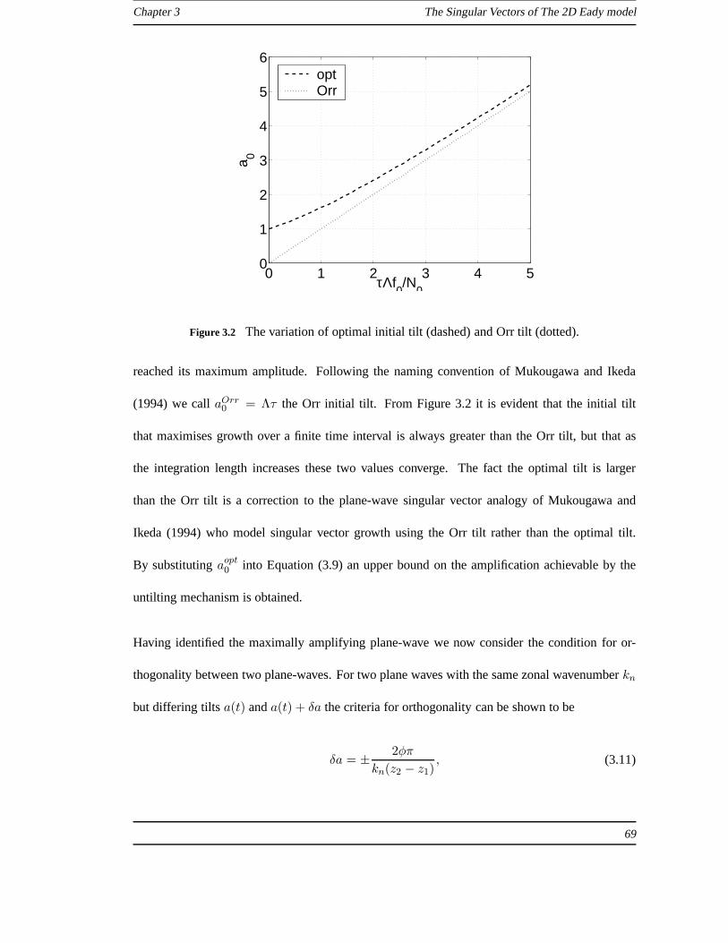
Chapter 3 The Singular Vectors of The 2D Eady model
0 1 2 3 4 50
1
2
3
4
5
6
τΛf0/N
0
a 0
optOrr
Figure 3.2 The variation of optimal initial tilt (dashed) and Orr tilt (dotted).
reached its maximum amplitude. Following the naming convention of Mukougawa and Ikeda
(1994) we callaOrr0 = Λτ the Orr initial tilt. From Figure 3.2 it is evident that the initial tilt
that maximises growth over a finite time interval is always greater than the Orr tilt, but that as
the integration length increases these two values converge. The fact the optimal tilt is larger
than the Orr tilt is a correction to the plane-wave singular vector analogy of Mukougawa and
Ikeda (1994) who model singular vector growth using the Orr tilt rather than the optimal tilt.
By substitutingaopt0 into Equation (3.9) an upper bound on the amplification achievable by the
untilting mechanism is obtained.
Having identified the maximally amplifying plane-wave we now consider the condition for or-
thogonality between two plane-waves. For two plane waves with the same zonal wavenumberkn
but differing tiltsa(t) anda(t) + δa the criteria for orthogonality can be shown to be
δa = ±2φπ
kn(z2 − z1), (3.11)
69

Chapter 3 The Singular Vectors of The 2D Eady model
whereφ 6= 0 is an integer. Proof of this relationship is given in Appendix B. Perturbations of
differing zonal wavenumbers are orthogonal to each-other due to the periodicity of the domain
in the zonal direction. Since the evolution of the tilt between two time-pointst1 andt2 is given
by a(t2) = a(t1) − Λ(t2 − t1), it can easily be verified that two plane-waves that satisfy the
condition for orthogonality given in Equation (3.11) at a given time pointt1, will still satisfy
the orthogonality condition at a subsequent time pointt2. To see this one simply need consider
two tilts at t1, a and a′(t1) = a(t1) ± δa respectively. Over the time intervalt1 to t2 both
tilts change by−Λ(t2 − t1), therefore att2 we may writea(t2) = a(t1) − Λ(t2 − t1) and
a′(t1) = a(t1) ± δa− Λ(t2 − t1) = a(t2) ± δa; i.e. the difference between the two tilts remains
fixed at±δa.
Several points may be inferred from the orthogonality and optimal growth/decay conditions de-
fined by Equations (3.10) and (3.11) respectively. Firstly,it is noted that, as is the case for singular
vectors, a set of orthogonal plane-waves will be orthogonalat both the beginning and end of a
finite time interval. Secondly we are free to choose one plane-wave in the set to be that which
maximises growth over the finite time interval, and using Equation (3.11) we may chose all sub-
sequent plane-waves to be orthogonal to it. In this way, we can define a discrete set of continuous
functions which share some of the properties of the singularvectors of a discrete set of equations.
From Equation (3.10) we can deduce that the difference in tilt between the optimally growing
and decaying plane-wave is given bya+0 − a−0 =
√
Λ2τ2 + 4N2
0
f2
0
. If the difference in the tilt of
optimally amplifying and decaying plane-waves satisfies the orthogonality criteria given in Equa-
tion (3.11), then both the optimally amplifying and decaying plane-waves will be contained in the
discrete set of orthogonal plane-waves. This condition canonly be satisfied for a discrete set of
values ofτ , since the orthogonality criteria yields a discrete set of tilts. It is worth noting that
70

Chapter 3 The Singular Vectors of The 2D Eady model
for this discrete set of finite time intervals the orthogonalplane-waves (if normalised) appear to
share several of the mathematical properties of the singular vectors of a discrete matrix; however
it must be stressed that we are not attempting to suggest thatthis set of orthogonal plane-waves
is analogous to singular vectors; we are rather motivating the contrived question: ’if the singu-
lar vectors structure and evolution were described entirely by the plane-wave untilting Equation
(2.36), what would we expect the properties of the singular vector spectrum to be?’. As we shall
see in Section 3.4, and as is evident in the work of other authors (Morgan (2001) for example),
the singular vectors are not of purely plane-wave. In answering this question we shall however
shed some light on the properties of singular vectors.
We have identified the optimal tilts for amplification and decay, but we have not yet considered the
amplification of the plane-waves orthogonal to the maximally amplifying/decaying plane-wave.
To shed some light on this topic Figure 3.3 (after Badger and Hoskins (2001)) shows the variation
of the stream-function amplification rate (y-axis) with tilt (x-axis). From Figure 3.3 it can be
seen that the maximum amplification and decay rates occur near a = 0 and that as|a| tends to
infinity the amplification rate tends to zero. Since the amplification rate tends to zero as the tilt
tends to infinity the amplification over a finite time intervaltends to unity as theinitial tilt tends
to infinity; Therefore for a finite time interval all the growing and decaying plane-waves will have
tilts ’near’ toa0 = 0. Mukougawa and Ikeda (1994) make the point that for discretemodels when
the integration length increases beyond a certain level theOrr initial tilt will require a vertical
wavelength smaller than the discrete model’s resolution. We may also make the point that for a
fixed integration if the vertical resolution is increased (relative to a fixed zonal resolution) beyond
a certain value then the newly resolved perturbations will not be able to grow via the untilting
mechanism. From a singular vector perspective this impliesthat if untilting accounts for the
71
Chapter 3 The Singular Vectors of The 2D Eady model
-4 -2 0 2 4
-2
-1
0
1
2
a0f0/N
0
(N0/Λ
f 0)∂ |ψ
|/∂ t
Figure 3.3 Untilting streamfunction/kinetic energy amplification rate; after Badger and Hoskins
(2001)
growth of singular vectors, then increasing vertical resolution will eventually lead only to the
addition of a large number of arbitrary (except in their orthogonality to the growing/decaying
singular vectors), ’essentially’ neutral singular vectors.
An important implication of Equation (3.11) for the amplification of plane-waves orthogonal to
the optimally amplifying plane-wave is that, sinceδa depends on1/kn, the difference in tilt
between two orthogonal plane-waves is smaller for high zonal wavenumbers. Since the differ-
ence between the tilts of orthogonal plane-waves is smallerfor high zonal wavenumbers than for
low zonal wavenumbers, the difference in growth rates between orthogonal plane-waves is also
smaller for high zonal wavenumbers than for low zonal wavenumbers. The increasing similarity
in the finite time amplification of orthogonal plane-waves with increasing wavenumber implies
that the amplification of the nearest (in terms of initial tilt) orthogonal plane-waves to the opti-
mally growing plane-wave will tend to the amplification of the optimally growing plane-wave, as
the zonal wavenumber tends to infinity. From a singular vector perspective one might expect that,
if plane-wave untilting explains much of singular vector growth, then the singular values associ-
72
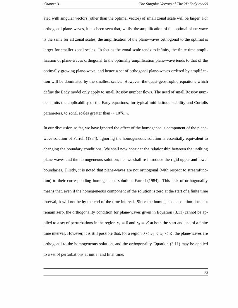
Chapter 3 The Singular Vectors of The 2D Eady model
ated with singular vectors (other than the optimal vector) of small zonal scale will be larger. For
orthogonal plane-waves, it has been seen that, whilst the amplification of the optimal plane-wave
is the same for all zonal scales, the amplification of the plane-waves orthogonal to the optimal is
larger for smaller zonal scales. In fact as the zonal scale tends to infinity, the finite time ampli-
fication of plane-waves orthogonal to the optimally amplification plane-wave tends to that of the
optimally growing plane-wave, and hence a set of orthogonalplane-waves ordered by amplifica-
tion will be dominated by the smallest scales. However, the quasi-geostrophic equations which
define the Eady model only apply to small Rossby number flows. The need of small Rossby num-
ber limits the applicability of the Eady equations, for typical mid-latitude stability and Coriolis
parameters, to zonal scales greater than∼ 103km.
In our discussion so far, we have ignored the effect of the homogeneous component of the plane-
wave solution of Farrell (1984). Ignoring the homogeneous solution is essentially equivalent to
changing the boundary conditions. We shall now consider therelationship between the untilting
plane-waves and the homogeneous solution; i.e. we shall re-introduce the rigid upper and lower
boundaries. Firstly, it is noted that plane-waves are not orthogonal (with respect to streamfunc-
tion) to their corresponding homogeneous solution; Farrell (1984). This lack of orthogonality
means that, even if the homogeneous component of the solution is zero at the start of a finite time
interval, it will not be by the end of the time interval. Sincethe homogeneous solution does not
remain zero, the orthogonality condition for plane-waves given in Equation (3.11) cannot be ap-
plied to a set of perturbations in the regionz1 = 0 andz2 = Z at both the start and end of a finite
time interval. However, it is still possible that, for a region0 < z1 < z2 < Z, the plane-waves are
orthogonal to the homogeneous solution, and the orthogonality Equation (3.11) may be applied
to a set of perturbations at initial and final time.
73

Chapter 3 The Singular Vectors of The 2D Eady model
By considering the vertical structure of the normal modes, we can gain some insight into the
relationship between plane-waves and the corresponding homogeneous solution. First, we shall
remind the reader that the homogeneous component of the plane-wave solution of Farrell (1984)
has the same vertical structure as the normal modes, but differing temporal behaviour. It is rea-
sonable to assume that the effect of the homogeneous solution on the untilting mechanism will be
weak at heights where the normal modes have small amplitude.As was seen in Figures 2.3A and
2.3B, the amplitude of normal modes associated with wavelengths below the short-wave cutoff
resides primarily above (below) the upper (lower) boundarysteering level, with some amplitude
extending into a region just below (above) the upper (lower)boundary steering level. Since the
amplitude of the normal modes is small between the upper and lower boundary steering levels, we
can infer that the effect of the homogeneous solution will berelatively weak in this region. Since
the steering levels are further apart for the smallest zonalscales, we can further infer that the size
of the region in which the homogeneous solution has only weakeffect is larger for smaller scales.
We may therefore expect the behaviour of small zonal scales to be closer to that of the plane-wave
particular solution given in Equation (2.36), than the large scales. For the longer wavelengths, the
normal modes have significant amplitude throughout the domain, so it would be expected that the
homogeneous component of the solution has large effect throughout the domain.
3.3.3 Modal unmasking
We have so far considered the implications of the plane-waveuntilting to singular vectors. In
this section we shall consider the implications of modal unmasking. A significant difference be-
tween potential vorticity unshielding and modal masking/neutral mode resonance is that whilst
the former depends on the relative positions of an infinite number of potential vorticity waves
74

Chapter 3 The Singular Vectors of The 2D Eady model
to one-anotherthe later depends on the relative position of the potential vorticity waves to two
specific normal modes. The limitation to dependency on the two particular modes means that
perturbations which amplify via the neutral mode resonanceand modal masking growth mecha-
nisms can only account for a small fraction of the model phasespace. The same can be said of the
exponentially growing normal modes which account for only one phase-space direction for every
zonal wavenumber.
Morgan and Chen (2002) consider the effects of modal maskingon the first singular vector for a
representative wavelength above the short-wave cutoff anda representative wavelength below the
short-wave cutoff. For the leading singular vectors presented by Morgan and Chen (2002), the
effect of modal masking is found to be very significant. In thecase of the singular vector below
the short-wave cutoff, Morgan and Chen (2002) point out thatthe amplitude of the normal mode
is masked by a relatively small number of the continuum modes. For this short-wave singular
vector, the potential vorticity associated with these continuum modes is a found to be plane-
wave perturbation located in a small region either side of the steering level. In the unmasking
mechanism described by Morgan and Chen (2002) the normal mode is revealed because of the
net cancellation of the continuum mode boundary potential temperature anomalies associated with
the potential vorticity anomalies above and below the steering level. Interestingly, despite the fact
that the largest amplitude potential vorticity waves reside on nearest discrete vertical levels to the
steering level, no linear amplification due to resonance is apparent, when the singular vector is
evolved far beyond the integration length used in the singular vector computation.
75

Chapter 3 The Singular Vectors of The 2D Eady model
De Vries and Opsteegh (2005) note that, for a single potential vorticity wave, the modal masking
effect is maximised if the potential vorticity wave residesat a distance
δz =π
knΛτ(3.12)
below (above) the upper (lower) boundary steering level. The motivation for the definition of
this expression lies in the fact that, if the potential vorticity resides at this height, the difference
in phase speeds between the normal mode and the continuum mode will lead to a change in
the relative phase of the continuum and normal mode of magnitudeπ. We shall call this the
optimal (modal) masking height. De Vries and Opsteegh (2005), however, do not consider the
implications for different zonal scales of this expression. From Equation (3.12) it is evident that
the distance of the optimal masking height from the steeringlevel is inversely proportional to the
integration lengthand to the wavenumber. The results of this inverse proportionality are three-
fold; firstly the distance from the steering level is smallerfor higher wavenumbers; secondly
the optimal masking height tends to the steering level height as the integration length increases;
thirdly the optimal masking height approaches the steeringlevel with increasingτ at a faster
rate at small zonal scales than large zonal scales. De Vries and Opsteegh (2005) find that the
optimal location of the single potential vorticity wave resides nearer to the steering level than
this optimal height for all integration lengths and conclude that resonance plays a greater role
than modal masking in the perturbation amplification. However, the findings of De Vries and
Opsteegh (2005) must be qualified by the fact that the perturbation is limited to initially have zero
potential temperature at the boundary.
Another point that is not discussed by De Vries and Opsteegh (2005) is that the amplification
achievable via modal masking by a potential vorticity wave residing at the optimal masking height
76

Chapter 3 The Singular Vectors of The 2D Eady model
will only lead to large amplification if the optimal masking height coincides with a height at which
the continuum mode can have large projection onto the normalmode. We can gain some insight
into the locations at which this may occur by considering theanalysis of Morgan and Chen (2002).
Morgan and Chen (2002) find that for small zonal scales ’only alimited number of (continuum)
modes (located near the steering level) are needed to mask the large amplitude of the neutral
edge modes’; whereas for large scales a ’broad distributionof continuum modes and the decaying
normal mode are required to mask the initially large amplitude of the growing normal mode. This
statement does not however preclude the possibility that a ’broad spectrum of continuum modes’
may also be used to mask an initially large amplitude normal mode.
Further insight can be gained by considering the structure of the continuum modes. Figures
3.4A to 3.4C show, for three representative wavelengths, the vertical profile (y-axis) of the
streamfunction-squared amplitude [Equation (2.32)] as a function of the height of the associ-
ated potential vorticity wave (x-axis). These figures were obtained from vertically discretising
the continuous continuum modes defined in Pedlosky (1964). For low wavenumbers (Figure
3.4A) the continuum modes always have large amplitude on theupper and/or lower boundaries
so modal masking can potentially occur if the optimal masking height is located anywhere in
the domain. For small scales (Figure 3.4C) the amplitude is large on the boundaries only if the
potential vorticity wave is located close to or above (below) the upper (lower) boundary steering
level. For intermediate scales (Figure 3.4B) the behaviourlies somewhere between that of large
and small scales. From this we may infer that modal masking can be an effective streamfunction
amplification mechanism for small zonal scales only when theoptimal masking height lies in this
region near the steering level. As we shall see later, in our analysis of the singular vectors, the
requirement that the optimal masking height coincides withthis near steering level region defines
77

Chapter 3 The Singular Vectors of The 2D Eady model
0.2 0.4 0.6 0.80
0.1
0.2
0.3
0.4
0.5
0.6
0.7
0.8
0.9
1
z0/Z
z/Z
0.1
0.2
0.3
0.4
0.5
0.6
0.7
0.8
0.9
A
0.2 0.4 0.6 0.80
0.1
0.2
0.3
0.4
0.5
0.6
0.7
0.8
0.9
1
z0/Z
z/Z
0.1
0.2
0.3
0.4
0.5
0.6
0.7
0.8
0.9
B
0.2 0.4 0.6 0.80
0.1
0.2
0.3
0.4
0.5
0.6
0.7
0.8
0.9
1
z0/Z
z/Z
0.1
0.2
0.3
0.4
0.5
0.6
0.7
0.8
0.9
C
Figure 3.4 Vertical profile (y-axis) of the streamfunction-squared amplitude [Equation (2.32)] of
continuum modes, as a function of the height of the associated potential vorticity wave (x-axis).
A: For wavenumbern = 2. B: For wavenumbern = 4. C: For wavenumbern = 7.
78
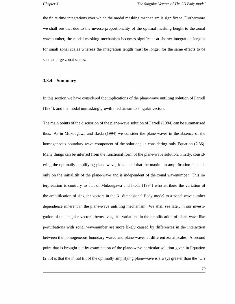
Chapter 3 The Singular Vectors of The 2D Eady model
the finite time integrations over which the modal masking mechanism is significant. Furthermore
we shall see that due to the inverse proportionality of the optimal masking height to the zonal
wavenumber, the modal masking mechanism becomes significant at shorter integration lengths
for small zonal scales whereas the integration length must be longer for the same effects to be
seen at large zonal scales.
3.3.4 Summary
In this section we have considered the implications of the plane-wave untilting solution of Farrell
(1984), and the modal unmasking growth mechanism to singular vectors.
The main points of the discussion of the plane-wave solutionof Farrell (1984) can be summarised
thus. As in Mukougawa and Ikeda (1994) we consider the plane-waves in the absence of the
homogeneous boundary wave component of the solution; i.e considering only Equation (2.36).
Many things can be inferred from the functional form of the plane-wave solution. Firstly, consid-
ering the optimally amplifying plane-wave, it is noted thatthe maximum amplification depends
only on the initial tilt of the plane-wave and is independentof the zonal wavenumber. This in-
terpretation is contrary to that of Mukougawa and Ikeda (1994) who attribute the variation of
the amplification of singular vectors in the3−dimensional Eady model to a zonal wavenumber
dependence inherent in the plane-wave untilting mechanism. We shall see later, in our investi-
gation of the singular vectors themselves, that variationsin the amplification of plane-wave-like
perturbations with zonal wavenumber are more likely causedby differences in the interaction
between the homogeneous boundary waves and plane-waves at different zonal scales. A second
point that is brought out by examination of the plane-wave particular solution given in Equation
(2.36) is that the initial tilt of the optimally amplifying plane-wave is always greater than the ’Orr
79

Chapter 3 The Singular Vectors of The 2D Eady model
initial tilt’. The fact that the optimal initial tilt is greater than the Orr tilt means that the optimally
amplifying plane-wave will continue to grow via untilting for a longer period of time than the in-
tegration length. The difference between the optimal initial tilt and Orr tilt is found to be greater
for short integrations than for long integrations.
The plane-wave particular solution of Farrell (1984) can beused to define a set of orthogonal
perturbations which remain orthogonal when evolved in time. For high zonal wavenumbers
the difference in tilt between orthogonal plane-waves is smaller than is the case for low zonal
wavenumbers. The similarity of the tilt of orthogonal high wavenumber plane-waves means that
the difference in finite time amplification between orthogonal plane waves is smaller for high
wavenumbers than small wavenumbers. However the plane-waves (unlike singular vectors) do
not form a complete set as the contribution to the phase spacefrom the homogeneous component
of the solution of Farrell (1984) must be taken into account.For high wavenumbers the structure
of the continuum modes associated with potential vorticitywaves in the region of the domain be-
tween the upper and lower boundary steering levels is similar to that which would be expected on
an infinite domain and it is inferred that plane-wave untilting can be used to entirely characterise
the stability properties of this region.
Whilst plane waves can account for a large number of phase space directions, perturbations that
lead to growth by modal unmasking are constrained to point only in phase space directions for
which the streamfunction field associated with the continuum modes can mask the streamfunction
field associated with the normal modes. It might be expected,therefore that modal unmasking will
be present in only as small number of the singular vectors.
It is hypothesised, that for the modal unmasking mechanism to lead to significant amplification,
80

Chapter 3 The Singular Vectors of The 2D Eady model
the optimal masking height [De Vries and Opsteegh (2005)] must reside in the region near to
the steering level. It is further hypothesised that, since this optimal masking height is inversely
proportional to the zonal wavenumber, modal unmasking willlead to significant growth in small
zonal scales at shorter integration lengths than is the casefor large zonal scales.
3.4 The singular vectors of the Eady model
3.4.1 A note on the indexing convention of the singular vectors
In the previous section, we examined the potential implications of different amplification mech-
anisms to the singular vectors of the Eady model. In this section we shall apply the information
outlined in the previous section to the singular vectors of the Eady model. We shall focus our
attention on the singular vectors computed for a12h and a48h integration.
Before this, to avoid confusion, we shall outline the singular vector indexing conventions that
we shall adopt throughout this section. In our discussions of the singular vectors, we shall adopt
the following conventions: we shall index the singular vectors of different zonal wavelengths
separately; each zonal wavelength/wavenumber shall be labelled by the wavenumber indexn,
where the wavenumber is given bykn = 2nπ/X; we shall label the singular vectors withi, with
i = 1 referring to the singular vector associated with largest singular value,i = 2 the second
largest; as an example, the firstn = 7 singular vector is the singular vector with wavenumber
indexn = 7 that is associated with the largest singular value.
81

Chapter 3 The Singular Vectors of The 2D Eady model
3.4.2 12h integration
Figures 3.5A to 3.5F show the right and left singular vectorsfor the first three wavenumber-index
seven singular vectors; i.e. the three largest amplifying singular vectors with zonal wavelength
X/7. These singular vectors form a regular structural pattern.The first singular vector is a
tilted plane wave structure with amplitude concentrated inthe centre of the domain. The second
comprises two tilted structures one on top of each-other andapproximatelyπ/2 out of phase.
The third has three tilted structures one on top of the other;the top and bottom structures are
anti-phased and the central structure is∼ π/4 out of phase. All the leading right singular vectors
have amplitude minima at the upper and lower boundaries. Thefourth, fifth etc singular vectors
(not shown) continue this pattern; the fourth having four plane wave structures, the fifth five
plane-wave structures etc. The corresponding left singular vectors follow this pattern but the tilt
is reduced and the amplitude on the upper and lower boundaries has increased relative to the rest
of the domain. This pattern qualitatively describes the structure of the leading singular vectors
at all wavelengths. There are, however, quantitative differences between the tilts and the vertical
structures. In what follows we shall outline these difference and how they are reflected in the
growth rates of the singular vectors.
Firstly, we consider the tilt of the potential vorticity field associated with the singular vectors. Fig-
ure 3.6A (blue line) shows the tilt of the leading singular vector for each zonal wavenumber. For
reference the black dotted line shows the Orr initial tilt and the black dashed line shows the opti-
mal initial tilt. The slight reduction in the optimal and Orrat high wavenumbers occurs because
the numerical phase speed (see Section 3.2.2) was used to calculate these tilts. At low wavenum-
bers, the initial tilt of the singular vectors is much largerthan the optimal tilt, but asymptotes to
the optimal tilt as the wavenumber increases. To understandthe effect of the initial tilt on the
82

Chapter 3 The Singular Vectors of The 2D Eady model
0 2 4 6 80
0.2
0.4
0.6
0.8
1
xf0/N
0Z
z/Z
-0.02
-0.01
0
0.01
0.02
A
0 2 4 6 80
0.2
0.4
0.6
0.8
1
xf0/N
0Z
z/Z
-0.02
-0.01
0
0.01
0.02
B
0 2 4 6 80
0.2
0.4
0.6
0.8
1
xf0/N
0Z
z/Z
-0.02
-0.01
0
0.01
0.02
C
0 2 4 6 80
0.2
0.4
0.6
0.8
1
xf0/N
0Z
z/Z
-0.02
-0.01
0
0.01
0.02
D
0 2 4 6 80
0.2
0.4
0.6
0.8
1
xf0/N
0Z
z/Z
-0.02
-0.01
0
0.01
0.02
E
0 2 4 6 80
0.2
0.4
0.6
0.8
1
xf0/N
0Z
z/Z
-0.02
-0.01
0
0.01
0.02
F
Figure 3.5 The leading three right and left12h singular vectors, for wavenumber indexn = 7.
A and B first right and left singular vector respectively. C and D second right and left singular
vector respectively. E and F third right and left singular vector respectively.
83

Chapter 3 The Singular Vectors of The 2D Eady model
amplification, Figure 3.6B shows the amplification of the singular vectors (singular values, black
line) and the theoretical amplification of a plane-wave (neglecting the effect of the homogeneous
solution, blue line) with the same initial tilt as the singular vector. For reference the black dashed
and dotted lines show the theoretical plane-wave amplification for the optimal and Orr initial tilts
respectively. Several things are noticeable from in Figure3.6B. Firstly, the amplification of all
the singular vectors (solid black line) is less than the maximum amplification implied by the op-
timal initial tilt (dashed black line). Since the singular vector amplification is less than that of
the optimal plane-wave it may be inferred that untilting is aless effective growth mechanism in
the presence of rigid upper and lower boundaries than in an infinite domain. Furthermore, since
the discrepancy is greater for small wavenumbers than high wavenumbers, it is possible that the
reduction in plane-wave amplification due to the homogeneous solution gets smaller as the space
between the steering level increases and the interaction between the interior potential vorticity
and the homogeneous components of the solution decreases. This hypothesis is partially born out
by the fact that the initial tilt of the singular vectors tends to that of the optimal plane-wave as the
wavenumber increases, suggesting that untilting is major factor in the amplification.
Further evidence can be gained by considering the distribution of streamfunction amplitude in the
vertical at initial (right singular vector) and final (left singular vector) time. Figures 3.7A and 3.7B
show the vertical distribution of streamfunction mean-squared amplitude (y-axis) for the leading
singular vectors of wave-indices one to ten (x-axis). Noticeably, at initial time, the amplitude is
largest in the central region of the domain for all wavenumbers. At final time, however, the long
wave singular vectors have amplitude distributed fairly evenly throughout the domain, whereas
for the shortest wavelengths the final time amplitude is still concentrated in the centre of the
domain. Figure 3.7C shows the potential vorticity squared amplitude for the leading singular
84
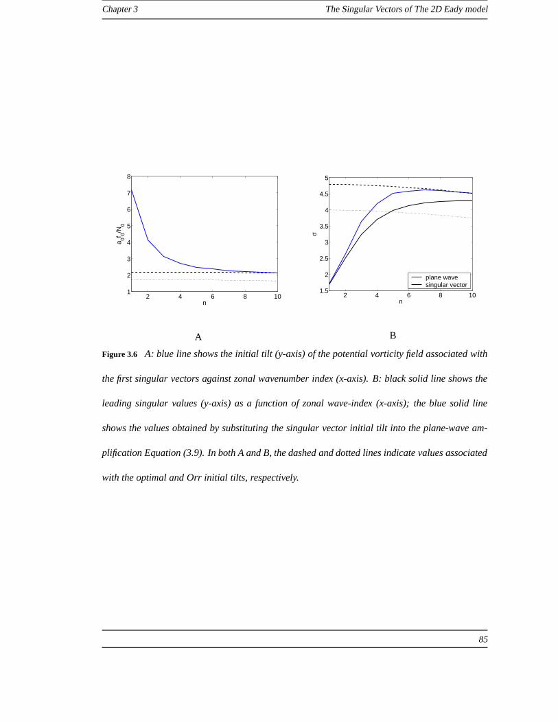
Chapter 3 The Singular Vectors of The 2D Eady model
2 4 6 8 101
2
3
4
5
6
7
8
n
a 0f 0/N0
A
2 4 6 8 101.5
2
2.5
3
3.5
4
4.5
5
n
σ
plane wavesingular vector
B
Figure 3.6 A: blue line shows the initial tilt (y-axis) of the potentialvorticity field associated with
the first singular vectors against zonal wavenumber index (x-axis). B: black solid line shows the
leading singular values (y-axis) as a function of zonal wave-index (x-axis); the blue solid line
shows the values obtained by substituting the singular vector initial tilt into the plane-wave am-
plification Equation (3.9). In both A and B, the dashed and dotted lines indicate values associated
with the optimal and Orr initial tilts, respectively.
85

Chapter 3 The Singular Vectors of The 2D Eady model
vector as a function of height and zonal wavenumber. For reference the blue dashed and solid lines
show the optimal masking height for the upper and lower boundaries respectively. The optimal
masking height is calculated using Equation (3.12). As withthe initial streamfunction field, the
potential vorticity field has maximum amplitude in the centre of the domain. For all wavenumbers
the optimal masking height does not lie in regions where it isexpected that the masking of the
normal modes by continuum modes will be large; in fact for thelowest wavenumbers the optimal
masking height lies outside of the domain. Since the optimalmasking height does not lie in
regions associated with potentially large masking of the normal modes by the continuum modes,
it may be inferred that modal masking is not the dominant amplification mechanism; that is not to
say that modal masking does not occur, but merely that its effect has not reached its full potential.
The fact that for small wavelengths the initial and final amplitude are both concentrated in the
centre in the domain indicates that the amplification is dominated by untilting of plane-waves
with high zonal wavenumbers; i.e. the amplification occurs in the locality of the of the potential
vorticity waves rather than on the boundaries.
We have already seen that for ’pure’ untilting plane-waves,the condition for orthogonality im-
plies that the plane-waves orthogonal to the optimally amplifying plane-wave will achieve larger
amplification for small zonal wavelengths than for large. Tosee if this property is also reflected
in the singular vectors we shall now consider the tilt of the singular vectors other than the first
singular vector. Figure 3.8A shows the initial tilts (y axis) of the first ten (right) singular vectors
(x axis) for different zonal wavenumbers. For ease of viewing only wave-indicesn = 1, 3, 5, 7, 9
(purple, light blue, red, green, dark blue respectively) are shown. As would be expected from
the orthogonality condition for plane-waves the tilt of thesingular vectors varies more rapidly
with singular vector index for low wavenumbers than for highwavenumbers. Figure 3.8B (blue
86

Chapter 3 The Singular Vectors of The 2D Eady model
1 2 3 4 5 6 7 8 9 100
0.2
0.4
0.6
0.8
1
n
z/Z
0.05
0.1
0.15
0.2
A
1 2 3 4 5 6 7 8 9 100
0.2
0.4
0.6
0.8
1
n
z/Z
0.06
0.08
0.1
0.12
0.14
0.16
0.18
0.2
B
1 2 3 4 5 6 7 8 9 10
0.2
0.4
0.6
0.8
n
z/Z
0.05
0.1
0.15
0.2
C
Figure 3.7 A: Streamfunction squared amplitude as a function of height(y-axis), for the first right
singular vectors of differing wavenumbers (x-axis shows wavenumber index); The black solid and
dashed lines show the lower and upper boundary steering levels respectively. B: Same as A, but
for left singular vectors. C: Same as A, but for potential vorticity, blue solid and dashed lines
show the optimal masking height for the lower and upper boundary steering levels respectively.
87

Chapter 3 The Singular Vectors of The 2D Eady model
line) shows the mean rate of increase in the initial tilt withsingular vector index as a function
of wavenumber. For reference the black line in Figure 3.8B shows the difference in tilt between
orthogonal plane-waves implied by Equation (3.11). It is noticeable in Figure 3.8B that these two
lines are closer together for high wavenumbers than for low indicating again that the behaviour of
singular vectors appears to be much closer to that of plane-waves at high wavenumbers than low
wavenumbers. Since the initial tilt of the singular vectorsvaries less rapidly with singular vector
index for high zonal wavenumbers, it would be expected that,due to the link between initial tilt
and amplification, the singular values also vary less rapidly. To see if this is the case, we con-
sidered the normalised ‘additive’ amplification of the singular vectors. The normalised additive
amplification is defined
‖Lvi‖ − ‖vi‖
‖Lv1‖ − ‖v1‖=σi − 1
σ1 − 1(3.13)
, and can be used to indicate the rapidity of descent of the singular value spectrum from the largest
singular value(σi − 1)/(σ1 − 1) = 1 to neutrality(σi − 1)/(σ1 − 1) = 0. Figure 3.9A shows
‘additive’ amplification of the12h singular vectors, as a function of singular vector index, for
each zonal wavenumber (for reference Figure 3.10 shows the actual singular values). From Figure
3.9A it is clear that the magnitude singular values decay less rapidly at higher wavenumbers than
at lower wavenumbers. As an example the blue line of Figure 3.9B shows the singular values
for n = 7 and the black line shows amplification inferred by substituting the initial tilts of the
singular vectors into the plane-wave amplification Equation (3.9). There is a striking similarity
in the shape of the black and blue lines in Figure 3.9B indicating that the reduction in singular
values with increasing ’i’ is due to the increasing initial tilt.
88

Chapter 3 The Singular Vectors of The 2D Eady model
1 2 3 4 5 6 7 8 9 100
10
20
30
40
50
60
i
a 0f 0/N0
n=1n=3n=5n=7n=9
A
1 2 3 4 5 6 7 8 9 100
2
4
6
8
n
(f0/N
0)δ a
0/δ i
singular vectorplane wave
B
Figure 3.8 A: Variation of initial tilt (y-axis) of the12h singular vectors, with singular vector
index (x-axis); each line corresponds to a different zonal wavenumber. B: The blue line show
the variation of the rate of change with respect to singular vector index (y-axis), with varying
wavenumber (a-axis); i.e. the blue line shows the gradientsof the lines in A; the black line shows
the value inferred from the condition for orthogonality forplane-waves Equation (3.11).
2 4 6 8 100
0.2
0.4
0.6
0.8
1
i
σ i-1/(
σ 1-1)
n=1n=2n=3n=4n=5n=6n=7n=8n=9n=10
A
1 2 3 4 5 6 7 8 9 101
1.5
2
2.5
3
3.5
4
4.5
5
i
σ i
plane wavesingular value
B
Figure 3.9 A: The normalised additive amplification of the singular vectors, as a function of
singular value index, for a12h integration. Each line represents a different zonal wavenumber.
B: Black line shows the singular values for the first tenn = 7 singular vectors; blue line shows the
amplification inferred by substituting the initial tilts ofthe singular vectors into the plane-wave
amplification Equation (3.9).
89
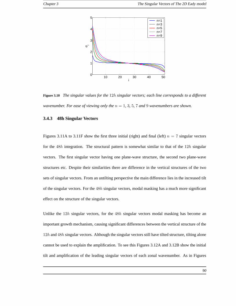
Chapter 3 The Singular Vectors of The 2D Eady model
10 20 30 40 500
1
2
3
4
5
i
σ i
n=1n=3n=5n=7n=9
Figure 3.10 The singular values for the12h singular vectors; each line corresponds to a different
wavenumber. For ease of viewing only then = 1, 3, 5, 7 and9 wavenumbers are shown.
3.4.3 48h Singular Vectors
Figures 3.11A to 3.11F show the first three initial (right) and final (left) n = 7 singular vectors
for the 48h integration. The structural pattern is somewhat similar tothat of the12h singular
vectors. The first singular vector having one plane-wave structure, the second two plane-wave
structures etc. Despite their similarities there are difference in the vertical structures of the two
sets of singular vectors. From an untilting perspective themain difference lies in the increased tilt
of the singular vectors. For the48h singular vectors, modal masking has a much more significant
effect on the structure of the singular vectors.
Unlike the 12h singular vectors, for the48h singular vectors modal masking has become an
important growth mechanism, causing significant differences between the vertical structure of the
12h and48h singular vectors. Although the singular vectors still havetilted structure, tilting alone
cannot be used to explain the amplification. To see this Figures 3.12A and 3.12B show the initial
tilt and amplification of the leading singular vectors of each zonal wavenumber. As in Figures
90

Chapter 3 The Singular Vectors of The 2D Eady model
0 2 4 6 80
0.2
0.4
0.6
0.8
1
xf0/N
0Z
z/Z
-0.02
-0.01
0
0.01
0.02
A
0 2 4 6 80
0.2
0.4
0.6
0.8
1
xf0/N
0Z
z/Z
-0.02
-0.01
0
0.01
0.02
B
0 2 4 6 80
0.2
0.4
0.6
0.8
1
xf0/N
0Z
z/Z
-0.02
-0.01
0
0.01
0.02
C
0 2 4 6 80
0.2
0.4
0.6
0.8
1
xf0/N
0Z
z/Z
-0.03
-0.02
-0.01
0
0.01
0.02
0.03
D
0 2 4 6 80
0.2
0.4
0.6
0.8
1
xf0/N
0Z
z/Z
-0.02
-0.01
0
0.01
0.02
E
0 2 4 6 80
0.2
0.4
0.6
0.8
1
xf0/N
0Z
z/Z
-0.03
-0.02
-0.01
0
0.01
0.02
0.03
F
Figure 3.11 The leading three right and left48h singular vectors, for wavenumber indexn = 7.
A and B first right and left singular vector respectively. C and D second right and left singular
vector respectively. E and F third right and left singular vector respectively.
91

Chapter 3 The Singular Vectors of The 2D Eady model
3.6A and 3.6B the black dashed and dotted lines give theoretical tilt and amplification values for
the optimal initial tilt and the Orr initial tilt respectively. Since for the high wavenumbers the
first singular vectors have two distinct tilted regions withdiffering tilts there are two blue lines
plotted: the sold blue line refers to the tilt of the potential vorticity in the centre of the domain
and the dash-dot line refers to the tilt of the maxima near optimal masking height. Looking first
at Figure 3.12A it is noticeable that the initial tilts of thesingular vectors both in the centre and at
the optimal masking height (blue lines) are significantly smaller than that implied by the optimal
and Orr initial tilts. In Figure 3.12B the blue lines denote the theoretical amplification obtained
by plane waves with same initial tilts as the singular vectors. The black solid line of Figure
3.12B gives the actual amplification achieved by the singular vectors; i.e. the black solid line
shows singular values. It is immediately apparent that the amplification of the singular vectors
far exceeds that suggested by their initial tilts. However it must be emphasised that this does not
imply that untilting makes no contribution to the overall amplification of the first singular vectors.
After-all there is still a relatively large amplitude tilted structure in the centre of the domain which
can have little impact on the evolution at the boundaries. What can be said however is that the
untilting mechanism no longer has as significant an impact onthe leading singular vector structure
as was the case for the12h singular vectors.
Figure 3.13 shows the vertical distribution of potential vorticity squared amplitude as a function
of wavenumber for the leading singular vectors. The blue line shows the optimal masking height
for upper and lower steering levels. In contrast to the12h integration the optimal masking height
for wavenumbers below the short-wave cutoff lies in the region which may lead to a large masking
effect. For the first singular vectors below the short-wave cutoff the potential vorticity has maxima
just below the upper boundary optimal masking height. For the lower boundary the potential vor-
92

Chapter 3 The Singular Vectors of The 2D Eady model
2 4 6 8 105
6
7
8
9
10
11
n
a 0f 0/N0
centremaximum
A
2 4 6 8 100
10
20
30
40
50
60
n
σ
svp.w. centp.w. max
B
Figure 3.12 As in Figure 3.6, but for the48hsingular vectors. A: blue line shows the initial tilt
(y-axis) of the potential vorticity field associated with the first singular vectors against zonal
wavenumber index (x-axis); the solid blue line shows the tilt in the centre of the domain, the
dashed blue line shows the tilt at the height the potential vorticity is maximised. B: black solid
line shows the leading singular values (y-axis) as a function of zonal wave-index (x-axis); the
blue solid line shows the values obtained by substituting the singular vector initial tilt into the
plane-wave amplification Equation (3.9). In both A and B, thedashed and doted lines indicate
values associated with the optimal and Orr initial tilts, respectively.
93

Chapter 3 The Singular Vectors of The 2D Eady model
ticity maxima lies just above the optimal masking height. The link between modal masking and
concentrations of Eady model singular vector potential vorticity near the steering level has been
discussed previously by Morgan and Chen (2002). By contrastDe Vries and Opsteegh (2005)
stress the importance of neutral mode resonance since they find that the singular vector potential
vorticity is always maximised nearer the steering level than the optimal masking height. What is
evident from the work presented here is that the importance of modal masking is dependent on
the relative sizes of the spatial scales and integration lengths considered. For example the poten-
tial vorticity structure of the leading12h singular vectors (Figure 3.7C) does not have maxima
near the optimal masking height. This lack of maxima is attributable to the fact that the optimal
masking height lies too far from the steering level for thereto be significant projection of the
continuum modes associated with potential vorticity at that height onto the normal modes. The
lack of such potential vorticity maxima does not mean that modal masking does not occur, only
that its effects are not large enough to cause significant deviation of the leading singular vector’s
structure from that of untilting plane-waves concentratedin the centre of the domain. By contrast,
the48h integration is long enough that the optimal masking height lies sufficiently close to the
steering level for the effects of modal masking on the leading singular vectors to be large. It must
be pointed out that the optimal masking height is dependent on both time and wavenumber. The
fact that strong effects of modal masking on leading singular vector structure are not seen for the
12h integration is in part attributable to the fact that only scales larger than800km are contained
in the spectrum. For smaller scales the optimal masking height will be (theoretically) closer to
the steering level and modal masking may be significant even for short integration lengths.
Figures 3.14A and 3.14B show the normalised additive amplification of the leading ten singular
vectors and the first twenty-five singular values for the48h integration, respectively. For ease
94

Chapter 3 The Singular Vectors of The 2D Eady model
1 2 3 4 5 6 7 8 9 10
0.2
0.4
0.6
0.8
n
z/Z
0.05
0.1
0.15
0.2
Figure 3.13 The vertical distribution of potential vorticity squared-amplitude of the first singular
48h singular vectors. The y-axis shows height, the x-axis showszonal wavenumber index. The
black and blue lines show the steering level and optimal masking heights respectively.
of viewing only then = 1, n = 3, n = 5, n = 7 andn = 9 singular values are shown in
Figure 3.14B. Several things are evident from these figures.Firstly, it can be seen in Figure
3.14A that the magnitude of the singular values descends less rapidly at high wavenumbers than
low wavenumbers, as was the case for the12h singular values (although the behaviour is slightly
more complex for wavenumbers smaller than the short-wave cutoff value). However, from Figure
3.14B it can be seen that, unlike the12h integration, the magnitude of the leading singular value
is not largest in the smallest scales. There are two possibleexplanations for this change in the
dependence of optimal amplification on zonal scale. Firstlythis may be attributable to the limited
vertical resolution of the model. Essentially since the model has limited vertical resolution the
resolvable tilts are also limited and for small zonal wavenumbers the limitations on tilt are more
severe; Mukougawa and Ikeda (1994). The fact that the optimal amplification is lower at the
smallest scales may be attributable to a reduction in the amplification attributable to the untilting
mechanism. A second explanation for this difference between optimal amplification over a12h
and48h integration is the variation in the structure of the continuum and normal modes with
95

Chapter 3 The Singular Vectors of The 2D Eady model
2 4 6 8 100
0.2
0.4
0.6
0.8
1
i
σ i-1/(
σ 1-1)
n=1n=2n=3n=4n=5n=6n=7n=8n=9n=10
A
5 10 15 20 250
10
20
30
40
50
60
i
σ i
n=1n=3n=5n=7n=9
B
Figure 3.14 A: The normalised additive amplification of the singular vectors, as a function of
singular value index, for a12h integration. Each line represents a different zonal wavenumber.
B: The48h singular values. Each line corresponds to a different zonalwavenumber.
zonal wavenumber. For high wavenumbers the normal and continuum modes are more confined
in the vertical and therefore interact in a smaller region. By contrast at lower wavenumbers there
structure is more ’spread out’ in the vertical so interact over a larger part of the model domain.
The limitation of the interaction at smaller scales to a smaller region of the domain may also lead
to a limitation in the maximum amplification. Which, if either, of these explanations is correct
will not be answered in the present work. What can be said however is that the difference in
optimal amplification between the different wavenumbers (apart from the lowest) is small relative
the magnitude of the amplification. Furthermore it shall be seen in the next chapter, that due to the
less rapid decent of the singular values associated with small scale singular vectors the cumulative
effect of all the singular vectors is still greater at smaller scales.
To gain further insight into the48h growing singular vectors as a whole we shall look more closely
at then = 7 singular vectors. Figures 3.15A and 3.15B show the streamfunction squared ampli-
96

Chapter 3 The Singular Vectors of The 2D Eady model
tude of the first ten initial (right) and final (left) singularvectors respectively. In Figure 3.15B the
singular vectors have been weighted by the singular values.Several things are noticeable from
Figures 3.15A and 3.15B. Firstly the leading few singular vectors are associated with a transfer
of amplitude from below the steering level to the upper and lower boundaries. By contrast the
streamfunction amplitude of the lower order singular vectors is similarly distributed throughout
the domain at both initial and final time. Whilst the leading few singular vectors have large am-
plitude maxima in the region just below the steering level the lower order singular vectors show
a slight weakening of amplitude in this region relative to the rest of the domain. For reference
Figure 3.15C shows the potential vorticity squared amplitude. In Figure 3.15C it can also be seen
that whilst the leading few singular vectors have large potential vorticity amplitude in the region
associated with unmasking effects the lower order singularvectors have a weakening of potential
vorticity in the ’unmasking region’. This difference structure in the unmasking region of the lead-
ing few and lower order singular suggests that the modal masking/unmasking mechanism leads
to amplification in only the few leading singular vectors.
Figure 3.16A shows the initial tilts of the first tenn = 7 singular vectors. The ’behaviour’ of
the tilts differs from that of the12h singular vectors in that the tilts do not increase linearly with
the initial tilt of the first singular vector being close to the optimal initial tilt. The tilts of the first
two singular vectors are similar and significantly smaller than the optimal initial tilt. After the
first two singular vectors the initial tilt increases linearly with at a rate similar (∼ 0.8f0/N0) to
the12h, untilting dominated, singular vectors. Figure 3.16B shows the singular values and the
value obtained from substituting the associated initial tilts of the singular vectors into the untilting
amplification equation. For the leading few singular vectors the singular values differ radically
from the amplification inferred from the untilting mechanism. For the lower order singular vectors
97

Chapter 3 The Singular Vectors of The 2D Eady model
1 2 3 4 5 6 7 8 9 100
0.2
0.4
0.6
0.8
1
i
z/Z
0.05
0.1
0.15
0.2
0.25
A
1 2 3 4 5 6 7 8 9 100
0.2
0.4
0.6
0.8
1
i
z/Z
2
4
6
8
10
12
14
B
1 2 3 4 5 6 7 8 9 10
0.2
0.4
0.6
0.8
i
z/Z
0.05
0.1
0.15
0.2
0.25
C
Figure 3.15 A: The streamfunction squared-amplitude as a function of height (y-axis) for the first
tenn = 7 right singular vectors. B: The streamfunction squared-amplitude as a function of height
(y-axis) for the first tenn = 7 left singular vectors, weighted by singular value squared.C: The
potential vorticity squared-amplitude as a function of height (y-axis) for the first tenn = 7 right
singular vectors; blue and black lines show the locations ofthe optimal masking height and the
steering level respectively.
98

Chapter 3 The Singular Vectors of The 2D Eady model
1 2 3 4 5 6 7 8 9 105
6
7
8
9
10
11
i
a 0f 0/N0
A
1 2 3 4 5 6 7 8 9 100
10
20
30
40
50
i
σ i
B
Figure 3.16 A: The initial tilts (y-axis) of the48h n = 7 singular vectors; x-axis shows the singular
vector index; the dotted and dashed black lines show the Orr and optimal initial tilts respectively.
B: The black line shows the48h n = 7 singular values, the blue line shows the amplification
implied by substituting the initial tilts of the singular vectors into the plane-wave amplification
Equation (3.9).
the behaviour is qualitatively more similar to that suggested by the untilting mechanism. The
fact that the lower order singular vectors do not lead to disproportionately large amplification
on the boundaries and that aside from the leading few singular vectors the initial tilt follows a
similar pattern to that of the12h singular vectors suggests that modal unmasking does not play a
significant role in any but the leading few singular vectors.
3.5 Summary
In this chapter we have examined the singular vectors of the 2D Eady model. Roughly speaking
we can infer the existence of two dynamical regimes for singular vectors. For short integration
lengths the untilting mechanism dominates the amplification. For the intermediate integration
99

Chapter 3 The Singular Vectors of The 2D Eady model
lengths, the modal unmasking mechanism is the dominant cause of amplification. In the next
chapter we shall discuss the implications of these two dynamical regimes to singular vector tar-
geting, but first we shall summarise the main characteristics of the two regimes.
In the untilting regime, the properties of the singular vectors may be summarised thus. The max-
imum amplification occurs at the shortest wavelengths. Additionally, the rate with which the
amplification decreases with increasing singular vector index is slower at smaller zonal wave-
lengths. The net result of this is that the ‘average’ amplification of smaller zonal scales is greater
than longer scales. For the untilting mechanism both the initial and final amplitudes tend to con-
centrated in the central vertical levels of the domain.
During the modal unmasking regime, the maximum amplification is not necessarily achieved by
the smallest zonal wavenumber. For singular vectors which amplify via modal unmasking the ini-
tial amplitude is concentrated near the steering level and the final amplitude is concentrated on the
boundaries. The transition from an untilting to a modal masking regime occurs when the integra-
tion length is sufficient for aπ phase change to occur in the relative phases of the normal modes
and the continuum modes near the steering level. This requirement implies that modal unmasking
will become significant more rapidly at small zonal scales than at large zonal scales. However,
since the modal masking regime relies on the normal modes, itcannot explain the growth of more
than a few singular vectors. Consequently even though modalunmasking is significant in de-
termining the structure of the leading singular vectors, during the modal unmasking regime the
untilting mechanism is still important to the singular vector amplification as a whole.
100
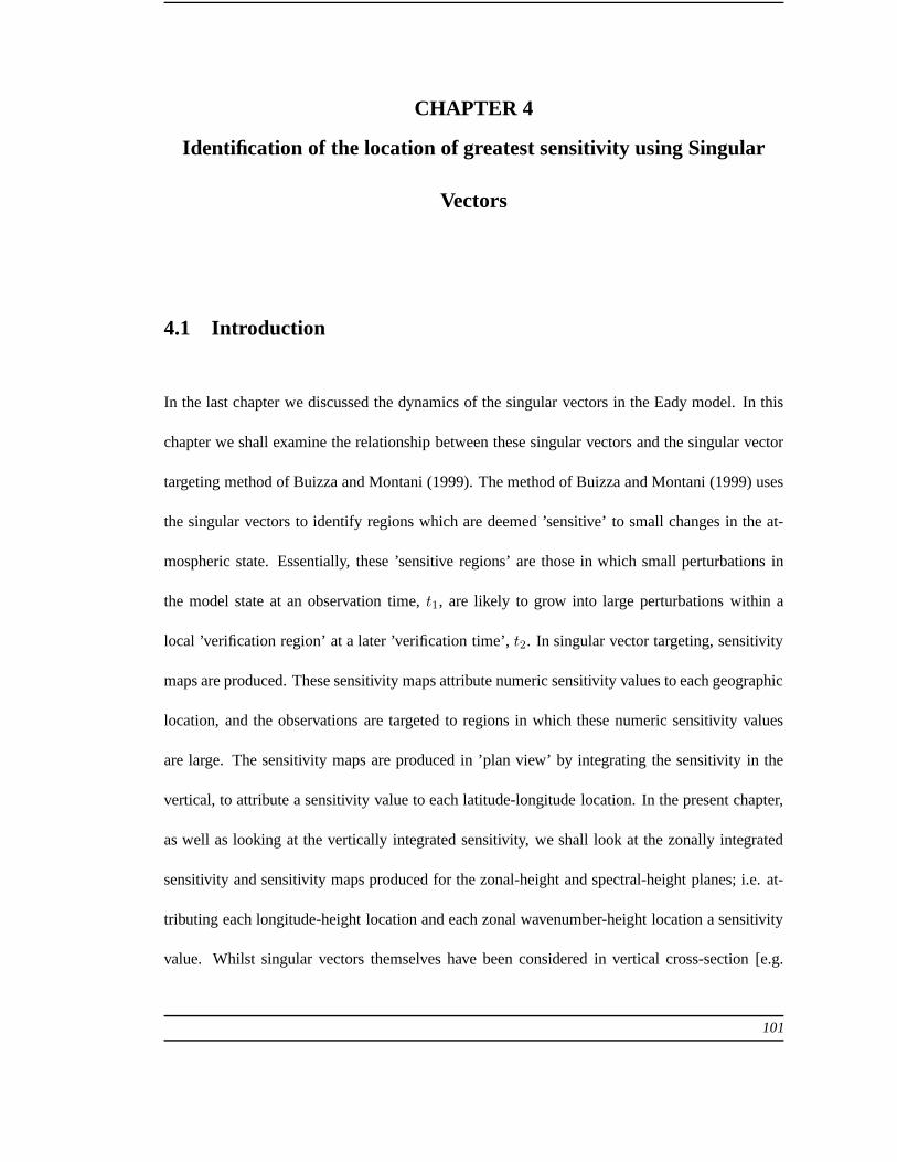
CHAPTER 4
Identification of the location of greatest sensitivity using Singular
Vectors
4.1 Introduction
In the last chapter we discussed the dynamics of the singularvectors in the Eady model. In this
chapter we shall examine the relationship between these singular vectors and the singular vector
targeting method of Buizza and Montani (1999). The method ofBuizza and Montani (1999) uses
the singular vectors to identify regions which are deemed ’sensitive’ to small changes in the at-
mospheric state. Essentially, these ’sensitive regions’ are those in which small perturbations in
the model state at an observation time,t1, are likely to grow into large perturbations within a
local ’verification region’ at a later ’verification time’,t2. In singular vector targeting, sensitivity
maps are produced. These sensitivity maps attribute numeric sensitivity values to each geographic
location, and the observations are targeted to regions in which these numeric sensitivity values
are large. The sensitivity maps are produced in ’plan view’ by integrating the sensitivity in the
vertical, to attribute a sensitivity value to each latitude-longitude location. In the present chapter,
as well as looking at the vertically integrated sensitivity, we shall look at the zonally integrated
sensitivity and sensitivity maps produced for the zonal-height and spectral-height planes; i.e. at-
tributing each longitude-height location and each zonal wavenumber-height location a sensitivity
value. Whilst singular vectors themselves have been considered in vertical cross-section [e.g.
101

Chapter 4 Identification of the location of greatest sensitivity using Singular Vectors
Hoskins et al. (2000), Montani and Thorpe (2002)], the linksbetween these singular vectors and
the calculation of sensitive regions have not been explicitly considered. By considering the sensi-
tivity in these different phase-planes we shall infer several points about the relationship between
the singular vector dynamics and the sensitivity in different locations.
Here it is worth re-iterating that the streamfunction norm used to compute the singular vectors
yields singular vectors identical to those that would result from a kinetic energy norm; Kim and
Morgan (2002). Since the streamfunction and kinetic energynorms give rise to identical singular
vectors all results in this chapter are consistent with either choice of norm; essentially by replacing
the word streamfunction with the word velocity throughout the chapter one can read the equivalent
analysis for kinetic energy. Since the structure of total energy and kinetic energy singular vectors
are found to be very similar in both the Eady model [Kim and Morgan (2002)] and more complex
models [Palmer et al. (1998)], it can be inferred that the streamfunction based sensitivity maps
considered in this chapter are consistent (in terms of the norm) with the total energy singular
vectors commonly employed in singular vector targeting.
As in the previous chapter, we shall constrain our discussions to only a12h and48h integra-
tion. We shall consider first sensitivity calculated for thenon-locally projected singular vectors
discussed in the previous chapter. We shall then turn our attention to sensitivity calculated for a
local ‘verification region’, using locally projected singular vectors. We shall see that the differ-
ence in the dominant dynamical mechanisms of these two integrations leads to differences in the
distribution of ‘sensitivity’ at the initial time. For the non-locally projected singular vectors, these
difference manifest themselves in the vertical distribution of sensitivity. For the12h integration
which is dominated by untilting, the sensitivity is maximised in the central vertical levels of the
domain. By contrast, for the modal unmasking dominated48h integration, the sensitivity is max-
102

Chapter 4 Identification of the location of greatest sensitivity using Singular Vectors
imised in two peaks close to the upper and lower boundary steering levels. In both cases however
the sensitivity remains greatest at shorter wavelengths. For the locally projected singular vectors
we shall see that the transition from the untilting regime tothat modal unmasking regime is also
associated with changes in the zonal distribution of sensitivity.
4.2 Sensitivity based targeting function
The use of singular vectors in targeting has usually been motivated from the perspective of sensi-
tivity or instability of the dynamical model in a particularregion. The motivation being that, by
correcting the initial conditions in the region in which thesubsequent forecast is most sensitive to
random excitation, it is expected that the forecast error will be maximally reduced. To be more
explicit the observations are deployed in regions where it is expected that randomly perturbing
the initial conditions will cause the greatest difference between the ’perturbed’ and ’unperturbed’
forecasts. For clarity, the term random perturbation in this context refers to a vector who’s ele-
ments are drawn from a symmetric statistical distribution with zero mean, and varianceγ. In this
section, we shall introduce a useful version of the ’typical’ implementation of singular vector tar-
geting which will be applied to the Eady singular vectors computed in the previous chapter. Here
we use the word ’typical’ since the implementation of ’singular vector targeting’ varies somewhat
between publications.
Given a localised random perturbation,T1δχ1, to the model state att1, we define the evolved
perturbation to be
δχ2(T1) = MT1δχ1. (4.1)
103

Chapter 4 Identification of the location of greatest sensitivity using Singular Vectors
δχ1 is a random vector whose elements are drawn from a zero mean symmetric statistical distri-
bution with varianceγ. The vectorT1δχ1 has random elements in the region defined by the local
projectionT1 and is zero outside this region. The evolved perturbationδχ2(T1) is defined as a
function of the local projectionT1 since it varies withT1 althoughδχ1 does not vary withT1.
With the above definitions the expected norm-squared amplitude of the perturbationT2δχ2(T1)
is given by
E[
‖T2δχ2(T1)‖2E2
]
= γ
Ng∑
i=1
σ2i v
Ti T1vi, (4.2)
wherevi andσi are theith right singular vector and singular value ofE1
2
2 T2ME− 1
2
1 respectively.
Equation (4.2) is essentially a prediction of the response in the region defined byT2 to randomly
perturbing the initial conditions in the region defined byT1. In singular vector targeting, the aim
is to identify the local projectionT1 from some restricted set that maximises Equation (4.2). The
use of such an expression to define a region for supplementaryobservations can be motivated
by suggesting that, if the inner product att1 used to define the singular value decomposition is
consistent with the initial condition errors, then Equation (4.2) is a prediction of the expected
error variance in the regionT2 at t2 that has its source inT1 at t1; Palmer et al. (1998). The idea
being that by placing observations in the region for whichE[
‖T2δχ2(T1)‖2E2
]
is maximised, the
reduction in the initial condition errors will lead to the greatest reduction in the forecast error
variance in the verification region.
The singular vector targeting found in publications such asBuizza and Montani (1999) and Leut-
becher et al. (2002) can be interpreted in terms of Equation (4.2). In these typical implementations
of singular vector targetingT1 is a projection onto all the grid points in the vertical column at a
particular latitude-longitude location. The targeting method is implemented by first calculating
104

Chapter 4 Identification of the location of greatest sensitivity using Singular Vectors
the values of Equation (4.2) for every such latitude-longitude location to produce a ’plan-view’
map of the sensitivity. The targeting region is then defined to include all latitude-longitude lo-
cations for which Equation (4.2) is greater than a certain fraction of the maximum; Buizza and
Montani (1999). One point to note is that the targeting described by Buizza and Montani (1999)
and Leutbecher et al. (2002) does not conform precisely to Equation (4.2). For example in some
cases Buizza and Montani (1999) define a sum the absolute amplitudes of the singular vectors in
the regionT1; and Leutbecher et al. (2002) sum over the elements singularvectors transformed
to ’total energy variables’ regardless of the inner productused in the singular vector computation.
Furthermore it must stated that whilst Equation (4.2) has a precise mathematical interpretation, it
is not necessarily the case for the singular vector targeting as implemented in publications such as
Buizza and Montani (1999) and Leutbecher et al. (2002). We have chosen to formulate the sin-
gular targeting method using Equation (4.2) because it has aprecise mathematical meaning and
enables a clear interpretation of the results of the idealised experiments contained in this work.
4.3 Sensitivity determined using non-locally-projected singular vec-
tors
4.3.1 12h integration
Firstly we consider the twelve hour integration. Figure 4.1shows a sensitivity map for the height
spectral phase plane. In order to produce this sensitivity map all the singular vectors were included
in Equation (4.2). Several things are evident from Figure 4.1. Firstly high zonal wavenumbers
have far greater sensitivity than low wavenumbers. This canbe seen more clearly in Figure
105

Chapter 4 Identification of the location of greatest sensitivity using Singular Vectors
1 2 3 4 5 6 7 8 9 100
0.2
0.4
0.6
0.8
1
n
z/Z
2.5
3
3.5
4
Figure 4.1 The sensitivity plotted in the height-wavenumber phase plane, for the12h integration.
4.2A which shows the sensitivity map integrated in the vertical. This increased sensitivity in the
smallest zonal scales can be interpreted in terms of the singular vectors discussed in Chapter 3.4.2.
In terms of the singular vectors there are two contributing factors to the increased sensitivity at
small zonal scales. The first is that the amplification of the optimally amplifying singular vector
is larger for high wavenumbers than low wavenumbers. The second contributing factor is that the
singular values decrease in amplitude less rapidly at smaller zonal scales. Both these points were
highlighted in the previous chapter.
The second thing that is evident in Figure 4.1 is that the model is most sensitive in the region
approximately bounded by the steering levels. Since the distance between the upper and lower
boundary steering levels increases with wavenumber, for high wavenumbers the sensitive area is
of greater vertical depth. Figure 4.2B shows the sensitivity as a function of height. From Figure
4.2B it can be seen that the sensitivity is maximised in a nearly uniform region spanning the
central half of the domain.
106
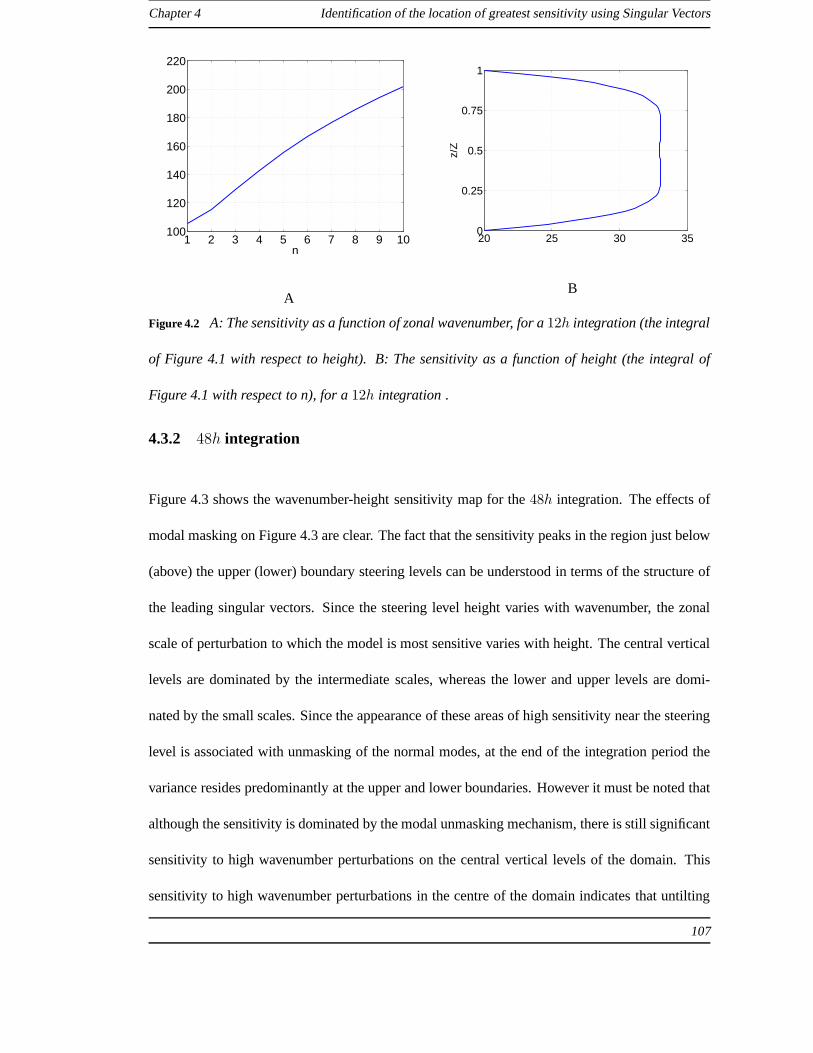
Chapter 4 Identification of the location of greatest sensitivity using Singular Vectors
1 2 3 4 5 6 7 8 9 10100
120
140
160
180
200
220
n
A
20 25 30 350
0.25
0.5
0.75
1
z/Z
B
Figure 4.2 A: The sensitivity as a function of zonal wavenumber, for a12h integration (the integral
of Figure 4.1 with respect to height). B: The sensitivity as afunction of height (the integral of
Figure 4.1 with respect to n), for a12h integration .
4.3.2 48h integration
Figure 4.3 shows the wavenumber-height sensitivity map forthe48h integration. The effects of
modal masking on Figure 4.3 are clear. The fact that the sensitivity peaks in the region just below
(above) the upper (lower) boundary steering levels can be understood in terms of the structure of
the leading singular vectors. Since the steering level height varies with wavenumber, the zonal
scale of perturbation to which the model is most sensitive varies with height. The central vertical
levels are dominated by the intermediate scales, whereas the lower and upper levels are domi-
nated by the small scales. Since the appearance of these areas of high sensitivity near the steering
level is associated with unmasking of the normal modes, at the end of the integration period the
variance resides predominantly at the upper and lower boundaries. However it must be noted that
although the sensitivity is dominated by the modal unmasking mechanism, there is still significant
sensitivity to high wavenumber perturbations on the central vertical levels of the domain. This
sensitivity to high wavenumber perturbations in the centreof the domain indicates that untilting
107

Chapter 4 Identification of the location of greatest sensitivity using Singular Vectors
1 2 3 4 5 6 7 8 9 100
0.2
0.4
0.6
0.8
1
n
z/Z
100
200
300
400
Figure 4.3 The sensitivity plotted in the height-wavenumber phase plane, for the48h integration.
is still of significance. Whilst the sensitivity of the central vertical levels is peaked at the interme-
diate zonal scales, it must be noted that the cumulative contribution to the sensitivity in the centre
of the domain from the untilting of small scales is of similarmagnitude to that the intermediate
scales.
Figures 4.4A and 4.4B show the sensitivity as a function of wavenumber and height respectively.
From Figure 4.4A one can see that the sensitivity is peaked inthe smallest zonal scales. From
Figure 4.4B one can see that the result of the transition froman untilting regime to a modal
unmasking regime is the appearance of two distinct peaks in the vertical sensitivity distribution.
In the next section we shall see that for sensitivity computed using zonally localised singular
vectors, this change in vertical sensitivity distribution, results in a change in the zonal sensitivity
distribution.
108

Chapter 4 Identification of the location of greatest sensitivity using Singular Vectors
1 2 3 4 5 6 7 8 9 100
2000
4000
6000
8000
10000
12000
n
A
0 500 1000 1500 2000 25000
0.25
0.5
0.75
1
z/Z
B
Figure 4.4 A: The sensitivity as a function of zonal wavenumber (the integral of Figure 4.3 with
respect to height), for a48h integration. B: The sensitivity as a function of height (theintegral of
Figure 4.3 with respect ton), for a 48h integration.
4.4 Sensitivity determined using locally projected singular vectors
4.4.1 Singular value decomposition
Previously we have computed the singular value decomposition of the Eady model integral prop-
agator without any local projection operator. In this section we shall be computing the singular
vectors with a final time local projection operator. Our mainpurpose is to demonstrate the effect
of the local projection on the sensitivity measure discussed earlier in the present chapter. How-
ever, prior to this we shall define the mathematical formalism of the singular value decomposition
and discuss briefly the character of the computed singular vectors.
As with the non-locally projected singular vectors we shalluse the matrixL ∈ RNg×Ng to de-
note an the integral propagator of an initialgrid-point streamfunction field to the corresponding
final grid-point streamfunction field. The final time local projection is performed by the matrix
P ∈ RNr×Ng . In addition to these two matrices, an additional initial time Fourier filter matrix
109

Chapter 4 Identification of the location of greatest sensitivity using Singular Vectors
F ∈ R2Nk×Ng is used to prevent the inclusion of wavenumbers lower thankn = 10. This addi-
tional matrix is necessary since the grid-point resolutionof the model is higher than that implied
by the spectral space spanned by the first ten wavenumbers. Whilst the unprojected singular vec-
tors all contain a single zonal wavenumber, the locally projected singular vectors are comprised of
multiple zonal wavenumbers. For the unprojected singular value decomposition the Fourier filter
matrix was also used, however it made no difference to the structure the singular vectors, other
than to set the singular values associated with shortwave singular vectors to zero. The locally pro-
jected singular vectors, however, have multiple zonal wavenumbers in individual vectors. Since
the singular vectors contain multiple zonal wavenumbers, the structure of the singular vectors
differs from those computed without the Fourier filter. Utilising both the initial Fourier filter and
the final local projection singular value decomposition is defined
PLF TF =
rank(PLF T F )∑
i=1
σiuivTi . (4.3)
Detailed discussion of the structure of the locally projected singular vectors will not be given. We
shall however summarise the basic properties here. The local projection matrix is used to define
the verification region. For all numerical experiments presented in this thesis the verification re-
gion shall be a region of zonal extentNZ/f0 and heightZ; i.e. a region of one Rossby radius
zonally which occupies the full height of the domain. For reference, Figure 4.5A shows the first
right locally projected singular vector for the12h integration. The vertical black lines denote the
boundaries of the verification region. Figure 4.5B shows thefirst right locally projected singular
vector for the48h integration. From Figures 4.5A and 4.5B the effects of the final local pro-
jection on the singular vector structure can be seen. The amplitude of the singular vectors are
concentrated in a tilted region of similar width to the verification region. The tilt of the region
110

Chapter 4 Identification of the location of greatest sensitivity using Singular Vectors
0 1 2 3 4 5 6 7 80
0.2
0.4
0.6
0.8
1
xf0/N
0Z
z/Z
A
0 1 2 3 4 5 6 7 80
0.2
0.4
0.6
0.8
1
xf0/N
0Z
z/Z
B
Figure 4.5 Examples of first right locally projected Eady model singular vectors. Black vertical
lines denote the boundaries of the verification region. A:12h integration. B:48h integration.
is larger for longer integration lengths. From a dynamical point of view this is not particularly
surprising since, as was seen in the previous chapter, the streamfunction field of the singular vec-
tors is strongly connected to the potential vorticity field.Due to the conservative advection of
the potential vorticity by the sheared mean zonal wind, the potential vorticity perturbations in the
tilted region will be advected into the vicinity of the verification region by the end of the integra-
tion. Consequently the streamfunction field is also concentrated in the vicinity of the verification
region at the end of the integration. Since for longer integration lengths the potential vorticity will
travel further over the integration, the tilt of the region is larger. Another property of the locally
projected singular vectors that differs from that of the unprojected singular vectors is that the lo-
cally projected singular vectors contain multiple zonal wavenumbers. As an example Figure 4.6A
shows the streamfunction-squared amplitude of the first right 12h singular vector as a function
height and wavenumbers.
111

Chapter 4 Identification of the location of greatest sensitivity using Singular Vectors
1 2 3 4 5 6 7 8 9 100
0.2
0.4
0.6
0.8
1
n
z/Z
1
2
3
4
5
x 10-3
A
1 2 3 4 5 6 7 8 9 100
0.2
0.4
0.6
0.8
1
n
z/Z
0.3
0.35
0.4
0.45
0.5
B
Figure 4.6 A: The streamfunction squared-amplitude of the first right locally projected12h sin-
gular vector. B: The sensitivity in the height-wavenumber phase plane computed from the12h
locally projected singular vectors.
4.4.2 Invariance of the spectral-height phase-plane sensitivity, to zonal localisa-
tions
The local projection defined in the previous section localises only the zonal coordinate, and not
the vertical coordinate. It has already been seen that the localisation changes the structure of
the singular vectors. Despite the change in singular vectorstructure, zonal localisation does not
alter the sensitivity of the model when viewed in the spectral-height phase plane. To illustrate
this point, Figure 4.6B shows the sensitivity computed fromthe 12h locally projected singular
vectors plotted in the spectral-height phase plane. Comparing Figure 4.6B to the equivalent com-
puted with unprojected singular vectors (Figure 4.1) it is apparent that the two are identical up
to a multiplicative constant. This multiplicative constant is related to the zonal extent (measured
in grid-points) of the verification region, and is given byNv/Nx, whereNv is the number of
gridpoints in the verification region.
112

Chapter 4 Identification of the location of greatest sensitivity using Singular Vectors
Since the locally projected singular vectors and non-locally projected singular vectors produce
identical sensitivity patterns in the spectral-height plane, we can infer that the dynamical proper-
ties of these two singular vector spectraas wholeare identical, even if individually the singular
vectors differ in a appearance. Due to this similarity, whenconsidering the dynamics from a
wave perspective, we may utilise the analysis of the dynamical properties of Eady model singular
vectors given in the previous chapter in discussions of the sensitivity patterns generated by the
locally projected singular vectors. It should also be notedthat when considering the sensitivity
as a function of wavenumber, and as a function of height, the sensitivity pattern obtained with
the locally projected singular vectors is also identical (up to a multiplicative constant) to those
obtained using the unprojected singular vectors shown in Figures 4.2A and 4.2B respectively.
4.4.3 Introduction of height-zonal correlation by zonal localisation
In this section we shall look at the sensitivity computed using the locally projected singular vectors
in zonal-height plane. Firstly we shall look at some of the general properties of the sensitivity
patterns in the zonal-height plane. Figures 4.7A and 4.8A show the zonal-height plane sensitivity
pattern, computed for a12h and48h integration respectively. For both integrations the sensitivity
lies in a tilted region of width approximately equal to the width of the verification region. From
a potential vorticity dynamics perspective, the sensitiveregion lies in the region from which the
potential vorticity will have been advected into the verification region at the end of the integration.
In a sense one could say that the sensitivity is ’untilted’ over the integration length.
As a result of the tilted structure of the sensitive region different zonal locations are colocated
with regions of sensitivity at different heights. For example looking at Figure 4.8A, one can
say that atxf0/N0H = 4 the sensitivity occurs at the central height of the domain, whereas at
113

Chapter 4 Identification of the location of greatest sensitivity using Singular Vectors
xf0/N0H = 2 the sensitivity occurs atz/Z ∼ 0.8. In this way we can attribute zonal variations
in sensitivity to vertical changes in the sensitivity, and hence attribute the sensitivity at different
zonal locations to different growth mechanisms and zonal scales. Here it is worth emphasising
that we use the term scale rather than wavelength/wavenumber since by definition the variations
in sensitivity we are referring to must be constructed of multiple wavelengths. To illustrate this,
Figures 4.7B and 4.8B show the sensitivity as a function of zonal coordinate for the12h and
48h integrations respectively. For the12h integration, there is a single peak corresponding to the
sensitive region at the central height of the domain. The fact that the greatest sensitivity occurs
in the centre of the domain is attributable to the fact that potential vorticity unshielding is the
dominant growth mechanism for the singular vectors. By contrast, for the48h integration (Figure
4.8B) there are two peaks. These two peaks correspond to the sensitive regions near the upper and
lower boundary steering levels of the shortest wavelengths. The two peaks are therefore associated
with the modal unmasking of the shortwave normal modes. To see this explicitly Figure 4.9 shows
the sensitivity plotted with the shortwaves filtered out viaa Fourier filter. Each line in Figure 4.9
gives the sensitivity calculated with the the scales smaller than wave indexn filtered from the
singular vectors; for example then = 1 line contains only the longest wave, whereas then = 10
line contains all ten wavenumbers and is identical to that shown in Figure 4.8B. From Figure 4.9
it can be seen that the longest zonal wavelengths are associated with sensitivity between the two
peaks in Figure 4.8B and the double peak does not appear untilthe smaller scales are added to the
sensitivity calculation. The implication is that the location of the peaks corresponds to a region
where the verification region forecast is highly sensitive to changes in the small scales close to
the upper and lower boundary steering level. Between the peaks the forecast in the verification
region is less sensitive to changes in the small scales, but is however more sensitive to changes in
the large scales than at the peaks.
114
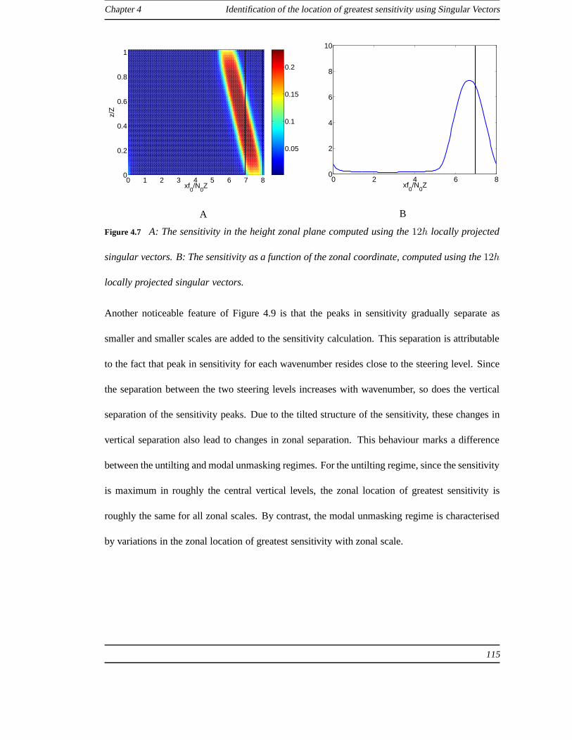
Chapter 4 Identification of the location of greatest sensitivity using Singular Vectors
0 1 2 3 4 5 6 7 80
0.2
0.4
0.6
0.8
1
xf0/N
0Z
z/Z
0.05
0.1
0.15
0.2
A
0 2 4 6 80
2
4
6
8
10
xf0/N
0Z
B
Figure 4.7 A: The sensitivity in the height zonal plane computed using the12h locally projected
singular vectors. B: The sensitivity as a function of the zonal coordinate, computed using the12h
locally projected singular vectors.
Another noticeable feature of Figure 4.9 is that the peaks insensitivity gradually separate as
smaller and smaller scales are added to the sensitivity calculation. This separation is attributable
to the fact that peak in sensitivity for each wavenumber resides close to the steering level. Since
the separation between the two steering levels increases with wavenumber, so does the vertical
separation of the sensitivity peaks. Due to the tilted structure of the sensitivity, these changes in
vertical separation also lead to changes in zonal separation. This behaviour marks a difference
between the untilting and modal unmasking regimes. For the untilting regime, since the sensitivity
is maximum in roughly the central vertical levels, the zonallocation of greatest sensitivity is
roughly the same for all zonal scales. By contrast, the modalunmasking regime is characterised
by variations in the zonal location of greatest sensitivitywith zonal scale.
115

Chapter 4 Identification of the location of greatest sensitivity using Singular Vectors
0 1 2 3 4 5 6 7 80
0.2
0.4
0.6
0.8
1
xf0/N
0Z
z/Z
2
4
6
8
10
12
A
0 2 4 6 80
50
100
150
xf0/N
0Z
B
Figure 4.8 A: The sensitivity in the height zonal plane computed using the48h locally projected
singular vectors. B: The sensitivity as a function of the zonal coordinate, computed using the48h
locally projected singular vectors.
4.5 Summary
In this chapter we have considered the sensitivity based singular vector targeting function of
Buizza and Montani (1999) in the context of the Eady model singular vectors computed in the
previous chapter. In the next chapter we shall introduce an extension to the singular vector tar-
geting method, that takes account of the data assimilation process, and the dynamical evolution
of errors prior to the forecast initialisation timet1. Firstly, we shall summarise the findings of the
present chapter.
The difference between the dynamical regimes of the short12h and intermediate48h integrations
leads to difference in the vertical distribution of sensitivity. In the case of the short integration,
untilting is the dominant growth mechanism, and consequently the sensitivity is concentrated in
the central vertical levels of the domain. By contrast for the intermediate integration the modal
116

Chapter 4 Identification of the location of greatest sensitivity using Singular Vectors
0 1 2 3 4 5 6 7 80
20
40
60
80
100
120
xf0/N
0Z
n=1n=2n=3n=4n=5n=6n=7n=8n=9n=10
Figure 4.9 The sensitivity as a function of the zonal coordinate, computed using the48h locally
projected singular vectors. The sensitivity is computed with the small zonal wavenumbers filtered
out. Each line corresponds to a different level of filtering,so for example, then = 1 line contains
only the longest zonal wavelength and then = 10 line contains all zonal wavelengths. N.B. the
n = 10 line is identical to Figure 4.8B.
117
Chapter 4 Identification of the location of greatest sensitivity using Singular Vectors
unmasking is the dominant growth mechanism, and consequently the sensitivity is concentrated
in two peaks near the upper and lower boundary steering levels of the shortest resolved zonal
wavelengths.
When the sensitivity to initial perturbations of a zonally localised verification region is consid-
ered, the difference between the two dynamical regimes of the short and intermediate integration
leads to differences in the zonal distribution of the sensitivity. These differences occur because
the sensitivity at a particular zonal location correspondsto the sensitivity of a small number of
vertical levels. Essentially this means that, when untilting is the dominant mechanism and the
sensitivity is greatest in the central vertical levels, thesensitivity is greatest at the zonal loca-
tion whose sensitivity depends the sensitivity of the central vertical levels. By contrast when the
modal unmasking regime is entered, the sensitivity is greatest at zonal locations whose sensitivity
depends the sensitivity of the vertical levels near to the upper and lower boundary steering levels.
Consequently for the untilting regime there is a single peak, whereas, when the modal unmasking
regime is entered, this peak separates into two zonally separated peaks.
118
CHAPTER 5
A singular vector targeting method that introduces dynamic
estimates of the initial condition errors
In this chapter we shall define an A-optimal [Berliner et al. (1999)] targeting method which
utilises singular vectors to obtain a reduced rank prediction of the observation locations that will
be of greatest benefit to the accuracy of the subsequent forecast. Rather than rely on the initial
normalising matrixE1, (following Berliner et al. (1999)) we shall approximate the initial con-
dition error statistics at timet1 by a transformation of a dynamically evolved background error
covariance matrix. Unlike Berliner et al. (1999), however,we shall define this transformation to
be consistent with the operational data assimilation system, and not an ensemble Kalman filter.
This difference in choice of transformation, leads to a significantly different final result.
By assuming an operational Kalman Filter, Berliner et al. (1999) arrive at a targeting function
that models the response obtained if the operational data assimilation were able to spread infor-
mation along the eigenvectors of the dynamically evolved background error covariance matrix.
By contrast, in the analysis presented in this chapter, we shall assume that the data assimilation
system contains a pre-specified model of the background error covariance which is not generally
consistent with the estimated actual covariance matrix. Making this assumption we shall define
a targeting function, the operation of which is summed up by Equation (5.18). The method es-
sentially finds the difference between the predicted forecast error variance, with and without the
observations, allowing for the fact that observations may increase or decrease the forecast error.
119

Chapter 5 A singular vector targeting
This work can be motivated by Bergot (2001), in which it is found that the impact of the targeted
observations is highly dependent on the quality of the background field. It is important therefore
that any targeting method should incorporate information about the background errors. Bergot
(2001) also find that only in cases where the observations were collocated with regions in which
the singular vectors used in targeting had non-negligible amplitude, do they have an effect on the
forecast error. This requirement of collocation with the region spanned by the targeted singular
vectors indicates that observations should not be placed outside this region. It is important to
note however that requiring observations to be collocated with the targeted singular vectors is
not the same as requiring that observations be located at thelocations where the singular vectors
have maximum amplitude; i.e. it is not a statement that the singular vector method described
in the previous chapter is the best means of selecting observation locations. It is simply that
regions where the singular vectors have negligible amplitude are dynamically disconnected from
the verification region. Bergot (2001) also find that the effectiveness of targeted observations
depends on the data assimilation system. It is therefore likely that consistency of the targeting
method with the operational data assimilation system is important.
In this chapter we shall first outline the statistical formulation of the targeting method. We shall
then consider how this targeting method may be approximatedusing singular vectors. Then we
shall consider the means by which the targeting method may bemade consistent with a hypothet-
ical operational data assimilation system. In the final section of this chapter we shall demonstrate
a simplified implementation of this targeting method in the Eady model, and discuss the connec-
tion between the target locations calculated and the dynamical analysis of the contained in the
previous chapters.
120

Chapter 5 A singular vector targeting
5.1 Basic formulation of a targeting method
In this section we define the basis for a targeting method. To form the basis of the method we
make the assumption that the expected background error covariance matrix att1 evolves from
the identity matrix at an earlier timet0, and that the error evolution fromt0 to t2 is linear. With
these assumptions a basic statistical formulation for the targeting method follows in a similar
fashion to that of Berliner et al. (1999). There is one significant difference between the statistical
formulation of Berliner et al. (1999) and that which we outline here. This difference is that
whilst Berliner et al. (1999) make the assumption that the observations are assimilated using
an (extended) Kalman filter, we make no such assumption. Rather than use the Kalman filter
equations, we define a matrix which is assumed in some way to approximate the gain matrix
(response function) of the operational data assimilation system.
We shall start our discussion by defining the background error covariance matrix att1. We make
the assumption that the background error covariance matrixat t1 is given by
B1 = ME−10 MT , (5.1)
whereM is the linear integral propagator for the intervalt0 to t1, andE−10 is a normalising matrix.
AssumingB1 takes this form is equivalent to assuming that the background error covariance
matrix evolves from a uniform, non-covariant, zero-mean distribution (with respect to theE0
inner product) att0; Berliner et al. (1999). Whilst we have definedM to be simply the linear
integral propagator, it is worth noting here thatM could in theory incorporate additional periodic
transformations to represent analysis cycles occurring betweent0 andt1.
The second component required for the targeting method is a means of transforming the back-
121

Chapter 5 A singular vector targeting
ground error covariance matrix att1 into the analysis error covariance matrix due to thepth
possible deployment of observations. For this purpose we define the matrixGp such that
A1(Gp) = GpB1GTp = GpME−1
0 MTGTp . (5.2)
The matrixGp is some approximation to the gain matrix (response function) of the data assimi-
lation system. The properties ofGp will be discussed in Section 5.3, but it is worth noting here
that in this definition ofA1 we have pre-emptively assumed that the effects of observation errors
on the analysis errors are small enough to be neglected.
Finally we require a means of evolving the analysis error covariance matrix att1 to the covariance
matrix of forecast errors in the verification region defined by the local projection operatorT2, at
t2. To produce this evolved covariance matrix we employ the matrix T2M , whereM is the linear
integral propagator for the intervalt1 to t2. The locally projected forecast error covariances are
then given by
T2B2(Gp)T2 = T2MGpB1GTpM
TT2 = T2MGpME−10 MTGT
pMTT2, (5.3)
where
B2(Gp) = MA1(Gp)MT (5.4)
is the predicted forecast error covariance matrices att2 for thepth deployment of observations.
Having defined the expected background errors due to thepth deployment of observations, the
next step is to define the metric by which the favourability ofthe deployment may be determined.
For this purpose we use the A-optimal measure of the expectedforecast error variance att2 as
122

Chapter 5 A singular vector targeting
measured with the norm induced by theE2 inner product. Following Berliner et al. (1999) we
note that the expected forecast error variance att2 is equal to the trace (sum of the elements on
the main diagonal) of the forecast error covariance normalised byE1
2
2 . The expected reduction in
forecast error variance due to thepth possible deployment of observations att1 is then given by
the reduction in the trace of the background error covariance matrix; i.e.
E[
‖T2ǫ2‖2E2
− ‖T2ǫ2(Gp)‖2E2
]
= traceE1
2T2B2(I)T2E1
2 − traceE1
2T2B2(Gp)T2E1
2
(5.5)
whereǫ2(Gp) andǫ2 denote the vector of forecast errors att2 obtained with thepth possible
deployment of observations and with no observations, respectively, and
B2(I) = MB1MT (5.6)
denotes the forecast error covariance matrix att2 when no observations are taken att1; i.e. if
Gp = I.
Here we have written the background error variance as the expectedE2-norm-squared amplitude
to facilitate comparison with the singular vector targeting criterion given in Equation (4.2) of
Chapter 4. As we shall see later, ift0 = t1 (i.e. M = I) and if a particularly simple choice of the
form ofGp is made, Equation (5.5) reduces to Equation (4.2).
Equation (5.5) defines the basis of the targeting method, however due to the high dimension of the
matrices involved, direct calculation ofE[
‖T2ǫ2‖2E2
− ‖T2ǫ2(Gp)‖2E2
]
for a singleGp is compu-
tationally expensive. The computational expense of calculating E[
‖T2ǫ2‖2E2
− ‖T2ǫ2(Gp)‖2E2
]
for multiple Gp would be extreme. Evidently Equation (5.5) requires significant simplification
before it may be used in practical targeting applications. In the next section we discuss the reduc-
123
Chapter 5 A singular vector targeting
tion of the dimension of the problem using singular vectors.In Section 5.3 we shall discuss the
properties of the matrixGp.
5.2 Using singular vectors to reduce the rank of the targeting prob-
lem
In the previous section we defined the basis of our A-optimal targeting method. The method re-
quires several high dimensional matrix operations to be performed recursively for different obser-
vational deployments. Such recursive calculations incur avast computational expense, therefore
a means of reducing the ’size’ of the problem is required. In this section we shall demonstrate
how singular vectors may be used to approximate the dynamical evolution of the errors leading,
to a large reduction in the computational cost.
We shall start by substituting into the definition ofE1
2
2 T2B2(Gp)T2E1
2
2 , the singular value decom-
position
E1
2
2 T2ME− 1
2
1 = UΣV T , (5.7)
whereU , V andΣ are matrices containing the left and right singular vectorsand the singular
values respectively. With this substitutionB2(Gp) becomes
E1
2
2 T2B2(Gp)T2E1
2
2 = UΣV TE1
2
1 A1(Gp)E1
2
1 V ΣUT (5.8)
We are however not interested in computation ofE1
2
2 T2B2(Gp)T2E1
2
2 . We are only interested in
calculation of the trace ofE1
2
2 T2B2(Gp)T2E1
2
2 . We can make use of the fact that the trace of a
124
Chapter 5 A singular vector targeting
matrix is invariant to similarity transformations (Golub and Van Loan (1983)) and write the trace
of E1
2
2 T2B2(Gp)T2E1
2
2 as
traceE1
2
2 T2B2(Gp)T2E1
2
2 = traceΣV TE1
2
1 A1(Gp)E1
2
1 V Σ. (5.9)
Here we have made use of the fact that sinceU is an orthogonal matrix (Golub and Van Loan
(1983)), U−1 = UT , and hence pre and post multiplication byU andUT respectively is a
similarity transformation. Writing the trace as the summation over the diagonal elements of
ΣV TE1
2
1 A1(Gp)E1
2
1 V Σ and using index notation for the matrix multiplications yields
traceE1
2
2 T2B2(Gp)T2E1
2
2 =
Ng∑
i=1
[ΣV TE1
2
1 A1(Gp)E1
2
1 V Σ]i,i
=
Ng∑
i=1
Ng∑
j=1
Ng∑
k=1
[ΣV T ]i,j[E1
2
1 A1(Gp)E1
2
1 ]j,k[V Σ]k,i
, (5.10)
where the notation[A]j,k denotes thejth element of thekth column of the matrixA. Noting that
theith row (column) ofΣV T (V Σ) is σivTi (σivi), we replace the summations overj andk with
matrix vector multiplications yielding
traceE1
2
2 T2B2(Gp)T2E1
2
2 =
r∑
i=1
σ2i v
Ti E
1
2
1 A1(Gp)E1
2
1 vi, (5.11)
wherer = rankE1
2
2 T2ME− 1
2
1
The next step is to simplifyA1(Gp). We start by noting that components ofA1(Gp) which lie
in the null-space (Golub and Van Loan (1983)) ofT2E1
2
2 M make no contribution to the trace of
E1
2
2 T2B2(Gp)T2E1
2
2 . Essentially this means that in regions which lie far from, or are ’dynamically
disconnected’ from the regionT2 att1, can be removed from the search for the optimal observation
locations. We define the local projection operatorT1 to contain all the geographical locations
125

Chapter 5 A singular vector targeting
which are to be included in the search.T1 is defined such that
T2MGpT1M = T2MGpM, (5.12)
for all potentialGp and consequently the trace ofE1
2
2 T2B2(Gp)T2E1
2
2 is unaffected by the pres-
ence ofT1; i.e.
traceE1
2
2 T2B2(Gp)T2E1
2
2 = traceE1
2
2 T2MGpME−10 MTGT
p MTT2ME
1
2
2 T2
= traceE1
2
2 T2MGpT1ME−10 MT T1G
Tp M
TT2ME1
2
2 T2
(5.13)
With this in mind we define the singular value decomposition
E1
2
1 T1ME− 1
2
0 =
r∑
j=1
σjuj vTj , (5.14)
wherer = rankT1E1
2
1 ME− 1
2
0 .
Making use of the orthogonality of the right singular vectors we may write
E1
2
1 T2ME−10 MT T2E
1
2
1 =
r∑
j=1
r∑
k=1
σjσkujvTj vku
Tk =
r∑
j=1
σ2j uju
Tj . (5.15)
Substituting the above into the trace ofE1
2
2 T2B2(Gp)T2E1
2
2 yields the expression
traceE1
2
2 T2B2(Gp)T2E1
2
2 =r
∑
i=1
r∑
j=1
σ2i σ
2jv
Ti E
1
2
1 GpE− 1
2
1 ujuTj E
− 1
2
1 GTp E
1
2
1 vi. (5.16)
Noting that this expression is the product of two identical inner products, we may write the trace
126

Chapter 5 A singular vector targeting
of E1
2
2 T2B2(Gp)T2E1
2
2 as
traceE1
2
2 T2B2(Gp)T2E1
2
2 =
r∑
i=1
r∑
j=1
σ2i σ
2j (v
Ti E
1
2
1 GpE− 1
2
1 uj)2. (5.17)
Finally, using Equation (5.17), we may writeE[
‖T2ǫ2‖2E2
− ‖T2ǫ2(Gp)‖2E2
]
in terms of the sin-
gular vectors as
E[
‖T2ǫ2‖2E2
− ‖T2ǫ2(Gp)‖2E2
]
=
r∑
i=1
r∑
j=1
σ2i σ
2j
[
(vTi uj)
2 − (vTi E
1
2
1 GpE− 1
2
1 uj)2
]
. (5.18)
The (vTi uj)
2 term comes about by noting that in the absence of observations Gp = I. By
rewriting in terms of the singular vectors we have reduced the computation expense to that of
r × r inner products for each possible deployment of observations. However the computational
expense will be reduced even further if Equation (5.18) is computed only approximately using
fewer thanr and r singular vectors. By computing Equation (5.18) with fewer singular vectors
we also reduce significantly the initial expense of computing the singular vectors.
We can interpret Equation (5.18) by considering the meanings of the two terms in the square
bracket. The first term,(vTi uj)
2, is a measure of the projection of the errors in the back-
ground field onto the ‘growing phase-space’ of the forecast error. It is by reducing this projection
that the assimilation of observations is expected to reducethe forecast error. The second term,
(vTi E
1
2
1 GpE− 1
2
1 uj)2 is a measure of the projection of the analysis errors associated with thepth
deployment of observations onto the growing phase-space ofthe forecast trajectory. If the first
term is larger than the second, then the Equation (5.18) is positive andpth deployment of observa-
tions is expected to be beneficial to the forecast accuracy. Conversely, if the second term is larger,
then Equation (5.18) is negative and the additional observations are likely to be detrimental to the
127

Chapter 5 A singular vector targeting
forecast accuracy. The idea that adding additional observational data will be detrimental to the
forecast may seem a little counterintuitive, but if one considers that reducing the errors in alocal
region acts as a rotation of theglobal error structure in phase-space rather than a simple global
reduction in error amplitude, it makes more sense. As a crudeexample one could consider simply
correcting the background error to the observation withoutany smoothing. Whilst this simple
correction procedure may reduce the initial condition error amplitude, it is likely create a ‘jagged’
error structure which may lead to greater error amplification than occurs in the uncorrected field. It
is the belief that the data assimilation process ’rotates’ the initial condition errors towards smaller
scales that in part motivates the type of singular vector based observation targeting described in
the previous chapter; Palmer et al. (1998). For our purposes, it is partly the possibility of obser-
vations causing ’unfavourable’ phase-space rotation of the errors that motivates both the desire
for Gp to be an approximation to the gain matrix of the operational data assimilation system, in
the evaluation of Equation (5.18). We shall show that this increase in forecast error would not be
predictable if the targeting method assumed the existence of an operational Kalman filter, as is
the case in methods such as the ensemble transform Kalman filter method. The desired properties
of Gp will be discussed more fully in the next section.
5.3 Approximation of the data assimilation response
In the previous sections of the current chapter we proposed amethodology for observation tar-
geting, and demonstrated how the computational expense of the method may be reduced. One
component of the methodology is the matrixGp, which is a transformation of the estimated back-
ground error covariance att1 to the predicted analysis error covariance matrix att1 due to thepth
128

Chapter 5 A singular vector targeting
possible deployment of observations. We have so far said very little about the desired properties
of Gp other than the fact it should approximate the response of theoperational data assimilation
system. Bergot (2001) find that the efficiency of targeted observations depends on the assimila-
tion scheme, noting several cases where the assimilation oftargeted observations by the 3D-Var
and 4D-Var schemes lead to significant differences in the change in accuracy of the subsequent
forecast. Bergot (2001) find that in some cases assimilationof observations with 4D-Var leads
to forecast improvement, whereas if 3D-Var is used, the assimilation of the same observations
degrades the accuracy of the subsequent forecast. The targeting methodologies of Bishop and
Toth (1999) and Hamill and Snyder (2002a) define the target region which would be beneficial
to forecast systems utilising ensemble Kalman filter based assimilation systems. At present me-
teorological centres typically employ 3D-Var and 4D-Var assimilation systems. The underlying
assumption of the existence of a Kalman filter may lead to miscalculations in the expected forecast
correction obtained from a given deployment of observations. Such mis-calculations have been
noted by Majumdar et al. (2001) who find the benefits of targeted observations are overestimated
by the Ensemble Transform Kalman Filter.
How Gp should be defined so that it is consistent with the operational data assimilation scheme
is a complex question. This question is further complicatedby the requirement that the gener-
ation of multipleGp and the subsequent calculation of the inner products in Equation (5.18) be
computationally inexpensive. We shall not attempt to tackle this question in full within this the-
sis. We shall instead demonstrate an inexpensiveGp for a simple 3D-Var assimilation system.
But prior to this we shall discuss some of the potential similarities and differences between the
effects of different assimilation schemes. We shall discuss first the properties of the 3D-Var and
4D-Var assimilation schemes that are used operationally inweather forecasting centres. We shall
129

Chapter 5 A singular vector targeting
also discuss the Kalman Filter. Although the Kalman Filter is not used operationally, Kalman
Filter theory is of particular importance to the targeting methods such as the Ensemble Transform
Kalman Filter.
In the 3D-Var assimilation scheme all observations within apre-specified finite time period (as-
similation window) are assumed to have been made at a single point in time. For example, if
we generate an analysis of the atmospheric state at the analysis timeta, in 3D-Var we treat all
observations made within a few hours ofta as if they were made atta. The cost function
J (χ) =1
2
(
χb − χa)T
B−1(
χb − χa)
+1
2(y −Hχ)T R−1 (y −Hχ) , (5.19)
which was introduced in Chapter 11 is then minimised (usually approximately) using an iterative
algorithm. In 3D-Var analysis schemes, the background error covariances are usually modelled
as separable in the horizontal and vertical directions, with the horizontal correlations assumed to
be homogeneous. The correlations between the errors in different variables and different hori-
zontal wavenumbers are often neglected. Due to the simplicity of the assumed background error
statistics, the 3D-Var assimilation scheme is effectivelyblind to the day to day variations in the ac-
curacy of the background field. In particular due to the homogeneity of the modelled background
error covariance 3D-Var ’spreads’ observational information evenly in all directions regardless of
any asymmetries in the correlations in the background errorstatistics.
The 4D-Var analysis scheme differs from the 3D-Var in that a linear integral propagator is in-
corporated into the definition of the forward model so thatH is replaced byHM(ta, to) where
M(ta, to) is the linear integral propagator from the analysis time,ta, to the observation time,
to. In the 4D-Var scheme the background error covariance matrix, B, is usually contains simi-
1For the definition in this chapter we have assumed that the observation operator/forward model is linear
130

Chapter 5 A singular vector targeting
lar approximations to those used in 3D-Var schemes. In 4D-Var, however, the inclusion of the
linear integral propagator means that observational information is spread in a manner more con-
sistent with the current atmospheric flow. In particular, due to the iterative solution methods used
to approximately minimise the cost function, 4D-Var preferentially adjusts the background field
along the leading singular singular vectors of the matrixM(ta, to). Essentially this means that
the change in the background field induced by observations isexpected to effect the structures
which amplify the most over the time intervalta to to. This picture is not so clear-cut, however,
since the degree to which the current dynamics affect the spreading of observational information
is dependent on the time intervalta to to. If the observations are made close to the analysis time
then the influence of the dynamics will be much lower than if the observations are made far from
the analysis time. For the former case, that of observationsbeing made close tota, the differences
between the response of a 4D-Var and a 3D-Var assimilation scheme with identicalB matrices
may be small.
In contrast to the 3D-Var and 4D-Var assimilation schemes, the Kalman Filter scheme does not
make assumptions of homogeneity of theB matrix. In the Kalman Filter scheme theB matrix is
continually evolved using the linearised dynamical model.Due to this continuous evolution of the
error statistics the Kalman Filter assimilation scheme takes account of large scale inhomogeneous
statistical correlations in the background errors which accumulate over time intervals longer than
the analysis windows used in 3D-Var and 4D-Var. For example the Kalman Filter may spread in-
formation along dynamical features such as fronts and cyclones; Majumdar et al. (2001). 3D-Var
and 4D-Var are only aware of these long range correlations inso much as they have been incorpo-
rated into the homogeneous model background error covariance matrix. Whilst the Kalman Filter
assimilation scheme is at present too expensive to be used inoperational weather forecasting it is
131

Chapter 5 A singular vector targeting
still relevant to targeted observations. This relevance isdue to the fact that targeting methods such
as the Ensemble Transform Kalman Filter and the ensemble method of Hamill and Snyder (2002a)
predict the forecast correction that would be obtained if the observations were assimilated using
Kalman Filter based data assimilation schemes. Essentially, these Kalman filter based methods
have the underlying assumption that the data assimilation scheme is ’aware’ of long range dy-
namical correlations specific to the current flow regime, when in actual fact the operational data
assimilation scheme may well be unable to account of such information. It is important to note
here that the fact the data assimilation scheme does not utilise information about long range dy-
namical error correlations does not mean such correlationsdon’t exist, merely that they do not
effect the ’spreading’ of observational information during the assimilation process. A targeting
method that does not make use of Kalman Filter theory may therefore give a more accurate pic-
ture of the response to the placement of observations in a given location. A targeting method
that assumes a 3D-Var or 4D-Var assimilation system may givea more accurate prediction of the
optimal observation locations. Consistency with the 3D-Var assimilation scheme may be more
easily achievable than consistency with the more complex 4D-Var scheme, but as has been noted
when the observation time is close to the analysis time thesetwo assimilation systems may be
relatively similar in their response. In the remainder of this section we shall define aGp which is
both consistent with a simple 3D-Var type assimilation scheme and computationally inexpensive.
We shall commence our definition ofGp by defining the analysis,χa, as the zero point of the
Jacobian (first derivative with respect toχ) of the cost function Equation (5.19). Taking the first
derivative and equating to zero yields
∂
∂χJ (χa) =
1
2B−1
(
χb − χa)
+1
2HTR−1 (y −Hχa) ≡ 0. (5.20)
132
Chapter 5 A singular vector targeting
We define the analysis, observation and background errors tobe the vector deviationsǫa = χt −
χa, ǫo = Hχt − y andǫb = χt − χb from the an imaginary perfect analysis (or ’truth’)χt.
Substituting these error definitions into Equation (5.20) and rearranging, we can write the analysis
errors
ǫa = (B−1 +HTR−1H)−1(B−1ǫb +HTR−1ǫo). (5.21)
From the above equation, we can see that the analysis errors are the sum of matrix transforma-
tions of the background and observation errors. If the observations are to be taken in regions with
large background errors, it is reasonable to assume that theamplitude of the background errors
will be larger than the observation errors, so we may simplify Equation (5.21) by lettingǫo = 0.
The effect of observation errors on the target selection could be included by adding an additional
term to the target selection Equation (5.18), however, for concision, discussion of this term will
not be included in this thesis. With this small observation error approximation, the analysis er-
rors are simply defined as a matrix transformation of the background errors. We can define the
transformation associated with thepth deployment of observations as
Gp = (B−1 +HTp R
−1p Hp)
−1B−1, (5.22)
whereHp andRp are the observation operator and observation error covariance matrix associated
with thepth deployment of observations. It is worth reminding the reader that the matricesR−1p
andB−1 are the error covariances assumed by the data assimilation system and are not neces-
sarily the same as the ’actual’ error covariance. Using theSherman-Woodbury-Morrison formula
133
Chapter 5 A singular vector targeting
(Golub and Van Loan (1983)) we may rewriteGp as
Gp = (B −BHTp R
− 1
2
p (I +R− 1
2
p HpBHTp R
− 1
2
p )−1R− 1
2
p HpB)B−1
= I −BHTp R
− 1
2
p (I +R− 1
2
p HpBHTp R
− 1
2
p )−1R− 1
2
p Hp
= I −BHTp (R +HpBH
Tp )−1Hp
= I −G′p,
(5.23)
where
G′p = BHT
p (R+HpBHTp )−1Hp. (5.24)
Substituting the above definition ofGp into the targeting criteria given in Equation (5.18) and
rearranging, yields
E[
‖T2ǫ2‖2E2
− ‖T2ǫ2(Gp)‖2E2
]
≃
≃
Nv≤r∑
i=1
Nu≤r∑
j=1
σ2i σ
2j
[
2(vTi uj)(v
Ti E
1
2
1 G′pE
− 1
2
1 uj) − (vTi E
1
2
1 G′pE
− 1
2
1 uj)2
]
.
(5.25)
If Nv = r andNu = r, then this is exactly equal to Equation (5.18), but if fewer thanNv = r
andNu = r singular vectors are used then the two equations are only approximately equal. After
the initial outlay of the singular vector computation, the computation of the target region requires
a singlecomputation of theNv × Nu inner products,vTi uj, plus the computation ofNv × Nu
inner products,vTi E
− 1
2G′pE
1
2 uj , for every observational deployment to be tested. The expense
of the inner productsvTi E
− 1
2G′pE
1
2 uj may be significantly reduced by exploiting the structure of
the matrix products which defineG′p. For example the matricesBHT
p andHTp Hp have the same
number of columns as there are observations. The number of non-zero elements in each column
will depend on the manner in which the observational information is spread by the data assimila-
134

Chapter 5 A singular vector targeting
tion system and the relationship between the observations and the control vector. In the simplest
case, if the control and observed variable are identical andthe background and observation error
covariance matrices are diagonal, thenG′p have only one non-zero element per observation. By
contrast, if the background and observation error covariance matrices are dense and the control
variable has a complicated relationship with the observed variable thenG′p will have a large num-
ber of non-zero elements. The complexity ofG′p determines the computational expense incurred
when testing each possible observational deployment. The simplerG′p the greater number of ob-
servational deployments that can be tested in a given time period. In the next Section we shall
define a simple data assimilation system to be used in the Eadymodel and the correspondingG′p.
5.4 Implementation of the targeting method in the Eady model
5.4.1 A simple definition ofGp
In this section we shall define a simple data assimilation system for the Eady model. We shall
then show the form of the correspondingGp based on the assumption that the observation errors
are small. We shall start by defining the control vector for the data assimilation system. We shall
define the control vector to be
χ = ψ = Fψ , (5.26)
whereF is the reduced rank Fourier transform introduced in the Chapter 3, andψ is the spectral-
space representation of the streamfunction field. Here is should be stressed that defining the
control vector in this way restricts the analysis increments to only contain the first ten zonal
wavenumbers. We shall further assume that all observationsare of streamfunction and collocate
135

Chapter 5 A singular vector targeting
with model grid2. The observation operator is then defined as the inverse Fourier transformation,
F T ∈ RNg×2Nk , from the spectral control-space to the grid point space followed by a projection,
Q ∈ RNo×Ng onto the grid points at which observations are located; i.e.
H = QF T . (5.27)
Following the conventions of 3D-Var we shall define the data assimilation system’s background
error covariance matrix such that the zonal and vertical correlations are separable, the zonal cor-
relations are homogeneous and isotropic and there are no correlations between different zonal
wavenumbers. With these assumptions, the background errorcovariance matrix consists of an
Nz ×Nz block for each zonal wave component. For the time being we shall not discuss the prop-
erties of the vertical correlations. Finally we shall make the assumption that the errors in different
observations are not correlated. Without correlations between observations the observation error
covariance matrixR ∈ RNo×No is diagonal. From Equation (5.21) the analysis errors for the
Eady model data assimilation system are defined as
ǫa = (B−1 + FQTR−1QF T )−1B−1ǫb + FQTR−1ǫo, (5.28)
and it follows thatG′p may be written
G′p = BFQT
p (Rp +QpFTBFQT
p )−1QpFT . (5.29)
2N.B. the reader is reminded that sinceF is not full rank, the model grid is of higher dimension than the Fourier
space associated with the first ten zonal wavenumbers
136

Chapter 5 A singular vector targeting
5.4.2 Simplification ofGp
Once the singular vectors have been computed, the only significant computational expense comes
from the inversion of the bracketed term(Rp +QpFTBFQT
p ) for multiple possible deployments
of observational deployments. Making use of the following:the observation errors vary with
height only; the background error covariance matrix is zonally homogeneous and isotropic; and
by neglecting the vertical background error correlations within the bracketed term, we may write
G′p
G′p ≃ BFQT
pD(z)QpFT , (5.30)
whereD(z) is a diagonal matrix whose elements depend on the height of the observation. Proof
of Equation (5.30) is given in Appendix C. Since, both(QF TBFQT )i,i and depend on height and
not the zonal location, the diagonal elements ofD depend only on the height of the corresponding
observation. The extent to which this approximation is valid depends on how close to being diago-
nalB actually is. Interestingly in ’typical’ 3/4d-Var assimilation schemes the vertical correlations
in B are strongest at low wavenumbers and on the upper and lower boundaries. By contrast, as
we shall see, the low wavenumbers and the upper and lower boundaries play only a minor role
in the selection of the target region using the method outlined above. Essentially this means that,
for typical assimilation schemes, the approximation ofB by its diagonal in the bracketed term is
likely to be most inaccurate in the regions of phase-space which are of least importance for the
target selection. That is not to say, however, that this in general a good approximation, merely
that the greatest inaccuracy occurs in the least significantregions.
At an even greater level of approximation, ifB andR are taken as uniform diagonal matrices (i.e.
137

Chapter 5 A singular vector targeting
constant multiples of the identity matrix) throughoutG′p then we may write
G′p ≃ cHT
p Hp = cFQTp QpF
T = cTp (5.31)
wherec is a constant andTp is a local projection operator that sets the model state to zero ev-
erywhere except at the observation locations. For this particularly simple definition ofG′p, when
t1 − t0 = 0, the targeting criteria given in Equation (5.25) reduces tothe same mathematical
formulation of the targeting criteria given in Equation (4.2). However whent1 − t0 is not equal
to zero then Equation (5.25) and Equation (4.2) are not of thesame mathematical form. For this
simple choice ofGp, the targeting criteria given in Equation (5.25) can be interpreted as an ex-
tension to Equation (4.2) in which the effect of the evolution of the errors prior to the observation
time is taken into account. In the next section we shall demonstrate a simple implementation
of Equation (5.25) in whichG′p = cTp and discuss the relationship to the results shown in the
previous chapter.
5.4.3 Computing the singular vectors
In this section we shall describe the implementation of the targeting method in the Eady model.
Firstly we need to define the singular vectors that will be used to compute the target region. As
in the previous chapter we shall define the singular value decomposition over the forecast period
from t1 to t2 thus,
P2LFT =
∑
i=1
σiuivi. (5.32)
138

Chapter 5 A singular vector targeting
For this first set of singular vectors the local projection isa projection onto the verification region.
For all calculations in this section the verification regionis selected to be the same as that used in
the previous chapter.
The second set of singular vectors are defined, over the interval t0 to t1 as
P1LFT =
∑
i=1
σiuivi, (5.33)
whereL is the integral dynamical propagator for the intervalt0 to t1, andP1 is a local projec-
tion. The local projectionP1 is defined to include all grid locations in which the ‘sensitivity’ as
identified by using the singular vector method of Buizza and Montani (1999) has non-negligible
amplitude.
5.4.4 Examination and dynamical interpretation of the optimal observation loca-
tion
In this section we consider the dynamical effects which determine the target regions calculated in
the Eady model using the new targeting method. We shall consider how the target regions vary
as the time intervalt0 to t1 is increased from zero. Since the target calculation fort1 − t0 = 0
yields the same results as the targeting method of Buizza andMontani (1999), we may use the
results to compare the targets calculated with the new method to those which would be computed
using that of Buizza and Montani (1999). The main aim of this section is to demonstrate how the
use of an additional set of singular vectors to approximate the statistics of initial condition errors
affects the location of the target region, and how this relates to the dynamics of the Eady model.
We shall consider two observing scenarios. These two scenarios are that a single vertical column
139
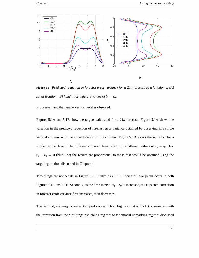
Chapter 5 A singular vector targeting
0 1 2 3 4 5 6 7 80
2
4
6
8
10
12
xf0/N
0Z
0h12h24h36h48h
A
-20 0 20 40 600
0.2
0.4
0.6
0.8
1
z/Z
0h12h24h36h48h
B
Figure 5.1 Predicted reduction in forecast error variance for a24h forecast as a function of (A)
zonal location, (B) height, for different values oft1 − t0.
is observed and that single vertical level is observed.
Figures 5.1A and 5.1B show the targets calculated for a24h forecast. Figure 5.1A shows the
variation in the predicted reduction of forecast error variance obtained by observing in a single
vertical column, with the zonal location of the column. Figure 5.1B shows the same but for a
single vertical level. The different coloured lines refer to the different values oft1 − t0. For
t1 − t0 = 0 (blue line) the results are proportional to those that wouldbe obtained using the
targeting method discussed in Chapter 4.
Two things are noticeable in Figure 5.1. Firstly, ast1 − t0 increases, two peaks occur in both
Figures 5.1A and 5.1B. Secondly, as the time intervalt1− t0 is increased, the expected correction
in forecast error variance first increases, then decreases.
The fact that, ast1−t0 increases, two peaks occur in both Figures 5.1A and 5.1B is consistent with
the transition from the ‘untilting/unshielding regime’ tothe ‘modal unmasking regime’ discussed
140

Chapter 5 A singular vector targeting
in the previous chapter. For values oft1 − t0 of order one to two days it may be inferred that the
effect of dynamical evolution of the errors is to push the initial condition errors further into the
modal unmasking regime. One can infer from this, that as was the case in the previous chapter,
the two peaks are associated with the smaller zonal scales close to the upper and lower boundary
steering levels, and that the area between the peaks is associated with the untilting of smaller
scales and the modal unmasking of the larger scales.
For the12h forecast the dynamical effect of evolved initial conditionerrors is greater, than for
the24h forecast. However this effect only leads to a double peak when observing for observing
different vertical levels; i.e. equivalent to Figure 5.1B,not shown. When observing a single
column, the location of the peak does not vary significantly.To understand this lack of variation
in the location of the peak for the12h forecast, one can consider that the tilt of the sensitive region
(see Figure 4.7A) is small, and consequently the regions associated with modal unmasking and
those associated with untilting/unshielding are in roughly the same zonal location. The result of
the coincidence of the regions associated with different growth mechanisms is that transition from
the untilting/unshielding regime to the modal unmasking technique does not significantly effect
the zonal location of the target region. For longer forecasts (e.g.48h), since the transition from
the unshielding to modal masking regime has largely occurred, the effect of changingt1 − t0 on
the location of the peaks is small. To see this explicitly, Figure 5.2B shows the variation in the
predicted reduction of forecast error variance obtained byobserving in a single vertical column,
with the zonal location of the column. In Figure 5.2B one can see that there is a small increase in
the distance between the peaks ast1 − t0 is increased. This lack of zonal variation in the location
of the optimal observation location, for12h and48h forecasts indicates that there is a ‘window’ of
forecasts durations, somewhere around24h, during which the zonal location of the target region
141

Chapter 5 A singular vector targeting
0 1 2 3 4 5 6 7 80
1
2
3
4
5
xf0/N
0Z
0h12h24h36h48h
A
0 1 2 3 4 5 6 7 80
10
20
30
40
50
60
xf0/N
0Z
B
Figure 5.2 Predicted reduction in forecast error variance as a function of height for (A) a12h
forecast, (B) a48h forecast, for different values oft1 − t0.
is sensitive to short term dynamically evolved perturbations. However this statement must be
qualified by the fact that the Eady model background state lacks the inhomogeneities present in the
dynamics of models linearised about time evolving forecasts trajectories. These inhomogeneities
may well lead to greater spatial variations in the optimal observation location with differingt1−t0.
Results from other authors [e.g. Snyder et al. (2003), Hamill and Snyder (2002b)] suggest that the
effects of inhomogeneities in the background state can havea significant impact on the structure
of linearly evolving covariances, over short time periods.Further investigation into the effect of
such spatial inhomogeneities on this simplified dynamical picture of targeting is required.
The second thing that is noticeable in Figures 5.1A and 5.1B is that, as the time intervalt1 − t0 is
increased, the expected correction in forecast error variance first increases, then decreases. This
behaviour is also seen in Figures 5.2A and 5.2B. Here the reader is reminded that the target is
normalised by the trace of the predicted back ground error covariance matrix att1, so that the
spatially averaged initial error variance is the same for each value oft1 − t0. The implication of
142
Chapter 5 A singular vector targeting
this increasing then decreasing expected reduction in error variance is that targeted observations
will be most effective if they correct errors that are dynamically evolved structures, but correcting
errors which are ‘too dynamically evolved’ will have lesserimpact. The implication is that there
is a value oft1 − t0 for which the impact of observations will be greatest. This value is likely
to vary with forecast length, so in order to make more generalcomments we have to consider
different forecast lengths. For this purpose, the dashed line of Figure 5.3 shows integral under the
curve (y-axis) of Figure 5.1A as a function oft1 − t0 (x-axis). The solid, dotted and dot-dashed
lines show the equivalent for12h 36h and48h forecasts respectively. Interestingly for all forecast
integrations, this increasing and decreasing effectiveness of observations with increasingt1 − t0
is observed. For longer forecasts the peak effectiveness occurs at smaller values oft1− t0, but for
all forecast lengths shown the peak occurs at a value oft1 − t0 greater than zero. Conversely, for
larget1 − t0 the effect of observations is smaller than for smallt1 − t0, implying that correction
of the long term evolved components of the forecast error mayhave lesser impact, than correcting
error components which are closer to random. However we muststress that this result comes
about because we have normalised the covariance att1. If we had normalised the error statistics
at t0, then the average error variance att1 would be larger for largert1 − t0, and the predicted
effectiveness of observations would increase with increasedt1 − t0.
5.5 Summary
In this chapter we have introduced a new singular vector targeting method and examined targets
produced using this new method using the Eady model singularvectors. This targeting method
gives a prediction of the reduction in forecast error variance that would be obtained from a given
143

Chapter 5 A singular vector targeting
0 12 24 36 480
100
200
300
400
500
600
t1-t
0
t2-t
1=12h
t2-t
1=24h
t2-t
1=36h
t2-t
1=48h
Figure 5.3 The variation of the predicted reduction in forecast error variance obtained by observ-
ing every location, as a function of the value oft1 − t0. Each line corresponds to a different
forecast lengtht2 − t1. For ease of viewing the values for the24h, 36h and48h forecasts have
been rescaled by factors1/2, 1/4, and1/8 respectively.
deployment of observations. The essential differences between this new method and previous
methods are that, it uses singular vectors to produce a dynamically determined estimate of the
initial condition errors, and that it utilises a linear transformation that can be made consistent
with the operational data assimilation system to approximate the effect of observations on the
initial condition errors.
In a simplified setting, the new targeting method is seen to coincide with the singular vector target-
ing of Buizza and Montani (1999). In this sense the new methodcan be interpreted as an extension
to ‘traditional’ singular vector targeting. In this chapter we examined the effect of including dy-
namically evolved initial condition error estimates into the singular vector targeting method. The
effect of including these evolved initial condition errorscan be interpreted dynamically as moving
the error evolution further into the modal unmasking regime. In a similar fashion to increasing
144

Chapter 5 A singular vector targeting
the forecast length in traditional singular vector targeting (see Chapter 4), increasing the length
of the dynamical evolution of the initial condition errors,leads to the appearance of double peaks
in the zonal and vertical sensitivity distribution. Furthermore it is found that the effectiveness of
observations is increased if they correct errors that have evolved over a short time period. If this
time period is increased or reduced, then the effectivenessof observations is reduced.
145

CHAPTER 6
Conclusions
This thesis is a contribution to the subjects of mid-latitude dynamics and targeted observations.
For the first time the full spectrum of singular vectors of theEady model are considered. The im-
portance and implications of the unshielding and modal unmasking mechanisms, to the computed
singular vectors are discussed. The computed singular vectors are used to analyse the singu-
lar vector targeting function commonly used in observationtargeting, in a vertical cross-section.
Through comparison of this vertical cross-section to the dynamics of singular vectors, inferences
about the scale and qualitative behaviour of the perturbations to which particular regions are ’sen-
sitive’ are made. In the final section of the thesis, a new targeting method is introduced. This new
targeting method utilises a set of evolved singular vectorsto approximate the background errors
within the region identified by a set of targeted singular vectors as dynamically connected to the
verification region. The two sets of singular vectors can then be used as a computationally inex-
pensive means of predicting the reduction of forecast errorvariance that will be obtained from a
given deployment of observations. In this final chapter we shall summarise the main results and
conclusions of the work in the thesis, as well as motivating future work which may follow from
that contained within the thesis.
In Chapter 3 we examined the properties of the full spectrum of singular vectors in the Eady
model. The results and conclusions of this chapter can be summarised as follows. Roughly
speaking we can partition the dynamics of the Eady singular vectors into two regimes. These two
146

Chapter 6 Conclusions
regimes are the untilting regime and the modal unmasking regime. For short integration lengths it
is found that untilting of potential vorticity is the dominant mechanism for singular vector growth.
As the integration length increases then modal unmasking increases in importance, eventually be-
coming the dominant growth mechanism. Whilst the importance of both these mechanisms to
singular vector growth has already been established by other authors, what has not been estab-
lished is the implications for these mechanisms for singular vectors other than the first, and the
significance of zonal wavenumber in setting the time-scale for the transition between the two
regimes.
For the untilting regime, it is found that the requirement for orthogonality between untilting struc-
tures means that at higher zonal wavenumbers the second, third etc singular vectors will have an
initial tilt closer to that of the first. This similarity of tilt means that the second, third etc short
wavelength singular vectors will have singular values closer to that of the first singular vector,
than would the equivalent longer wavelength singular vectors. Furthermore, it is found that for
short integrations the singular values at smaller zonal scales are closer to that suggested by the
untilting mechanism, whereas at longer scales they are significantly smaller. This discrepancy is
attributed to the fact that at the smaller scales the normal modes are shallower so the interaction
between the potential vorticity dynamics and that of the normal modes is lower than in the larger
scales, allowing for the untilting of potential vorticity to occur in the smaller scales more freely
at smaller scales. Taking into account both these scale selective effects, it may therefore be said
that, for the untilting regime, the smaller scales dominatethe singular vector spectrum because
their maximum growth is larger, and because there are a larger number of singular vectors which
achieve large amplification.
It is found that the modal masking regime which is characterised by concentrations of singular
147

Chapter 6 Conclusions
vector amplitude near the steering level allows for amplification which can exceed the maximum
amplification possible via untilting. The transition from the untilting to the modal masking regime
is shown to occur more rapidly at the smaller zonal scales than the larger zonal scales. The time-
scale for the transition is found that to depend approximately on the relative phase speeds of the
normal modes and the potential vorticity in the region in which there is a strong interaction be-
tween potential vorticity and the normal modes. For short integrations this phase difference is
too small to lead to a significant change in the phase of the normal and continuum mode. As the
integration length increases the difference in phase speedbetween the normal modes and the po-
tential vorticity waves which interact with them is sufficient to allow a ’half-period’ phase change
to occur. The integration length required for this requirement to be met is inversely proportional
to the wavenumber, therefore the smaller zonal scales will make the transition from the untilting
to the modal masking regime at a shorter integration length than the larger scales. An interesting
result of the scale selectivity of this transition is the fact that for models with very high resolu-
tion one would expect that the smallest scales will have entered the modal masking regime even
at very short integration lengths, leading to singular vectors with the amplitude of the smallest
scales concentrated at the steering level.
In Chapter 4 we examine the singular vector targeting methodin the context of the Eady model
singular vectors. By examining the ’sensitivity’ as identified in the zonal-height plane we are
able to make the following links between the singular vectordynamics and the sensitivity at dif-
ferent longitudes. During the untilting regime, there is only a single peak in sensitivity which
corresponds to untilting perturbations on the central vertical levels of the model. Since the sin-
gular vectors amplify via untilting, the peak in sensitivity is associated with the most sensitive
region for all zonal scales. As the integration length increases and the dominant growth mecha-
148

Chapter 6 Conclusions
nism tends to modal unmasking, then the zonal location of sensitivity of smaller scales diverges
from that of larger scales. The sensitivity to smaller scales occurs at two peaks ’near too’ and
’far from’ the verification region. These two peaks are associated with unmasking the normal
modes on the lower and upper boundaries, respectively. The sensitivity at longitudes between
these peaks is associated with the unmasking of the longer-wave normal modes and the untilting
of shorter wavelengths. The association of different locations with different scales/growth mech-
anisms is of particular significance to singular vector targeting of this kind, as whilst the targeting
method identifies target regions, it does not yield information on how to deploy observations in
these regions. Knowledge of the perturbation scales and structures to which these ’sensitive re-
gions’ are sensitive may increase the ability to make informed choices about actual observational
deployment, within the context of the established singularvector method.
In Chapter 5 we introduce a new singular vector targeting method. This targeting method dif-
fers from previous singular vector targeting methods, in that it utilises a dynamical estimate of
the initial condition errors, rather than assuming that these errors are random with respect to a
chosen inner product. It differs from the Ensemble Transform Kalman Filter (ETKF) in that it
utilises singular vectors that are computed to only containinformation dynamically relevant to
the verification region, rather than a non-linear evolved ensemble, which potentially contains lit-
tle information relevant to the verification region. Also unlike the ETKF, the validity of method
also does not require the user to assume the presence of an operational Ensemble Kalman Filter,
but rather allows the user to utilise any desired level of approximation to the operational data as-
similation system in the estimate of the forecast error variance reduction. One further difference
between the method and both the singular vector and ETKF methods, is that it explicitly predicts
the reduction in forecast error variance as the difference between the forecast error variance with
149

Chapter 6 Conclusions
and without the targeted observations. This additional feature introduces the potential for the pre-
diction of instances where adding observations is likely tolead to anincreasein the forecast error
variance in the verification region.
The targets identified using the new targeting method in the Eady model with simplified data
assimilation system are calculated. The target region is found to always reside somewhere within
the sensitive region identified by the traditional singularvector methods, however the location
of the best observation varies when the time-scale of dynamically evolved initial condition error
estimate is varied. As with the ‘traditional’ singular vector targeting method discussed in Chapter
4, the changes in the optimal observation location are induced by the transition from the untilting
to the modal unmasking regime. However unlike the traditional singular vector targeting method,
in the new method the transition from the untilting to the modal unmasking regime occurs through
evolution of the initial condition errors prior to the forecast initialisation time, rather than due an
increase in the duration of the forecast. It is also found that the forecast error is more sensitive to
corrections in initial condition errors that have evolved over a short time interval, than those which
have not evolved or those which have evolved over a longer time interval. This result is based on
the assumption that in each case the initial condition errors have the same average variance.
The work in this thesis has concentrated on the analysis of perturbation amplification and targeting
observations within the context of the Eady model. Whilst the simplicity of the Eady model
facilitates analysis, it is of interest to see how the results can be extended to more complex models.
Of particular interest is the relationship between the two dynamical regimes of the Eady model
singular vectors and the dynamical regimes identified in theECMWF model singular vectors by
Hoskins et al. (2000). A further consideration is the relationship between the targets identified
using the Eady singular vectors and those computed using singular vectors obtained from a time
150

Chapter 6 Conclusions
varying background state.
Another area in which this work could be extended is that of data assimilation. The targeting
method defined in Chapter 5 utilises a linear transformationto approximate the effect of data as-
similation on the initial condition errors. Whilst in principle this transformation could be highly
representative of the data assimilation system, in our results we have reduced it to a simple lo-
cal projection. One question that remains unanswered is, how similar does this transformation
have to be to the operational data assimilation system for the targeting method to be successful,
and furthermore how significant will the difference betweenthe targets calculated with the new
method be to those calculated using a Kalman filter based targeting method.
151

APPENDIX A
The Numerical Eady Model
A.1 Non-Dimensionalisation and Co-Ordinate Change
For the purpose of numerical accuracy, the Eady Equations outlined in Chapter 2 are non-
dimensionalised. The zonal, vertical and temporal coordinates (x, z andt) are rescaled by divisors
LR = N0Z/f0, Z andN0/f0Λ, respectively. A summary of the resultant rescaling applied to
different variables is given in TableA.1. In non-dimensional form Eady Equations are
∂q′
∂t= −ˆug
∂q′
∂x,
x ∈ [0, X ]
z ∈ (0, Z)
, (A.1)
∂b′
∂t= −ˆug
∂b′
∂x+ v′,
x ∈ [0, X ]
z = 0, z = Z
, (A.2)
where
q′ =∂2ψ′
∂x2+∂2ψ′
∂z2
x ∈ [0, X ]
z ∈ (0, Z)
, (A.3)
where
b′ =∂ψ′
∂z(A.4)
152

Appendix A The Numerical Eady Model
and
∫ X
0ψ′dx = 0, z ∈ [0, Z], (A.5)
where the hat denotes the non-dimensional variables. To minimise the variation in the magnitude
of the mean zonal wind over the domain the zero point is moved to the centre of the domain. The
mean zonal wind field may therefore be written
ˆug = z −Z
2. (A.6)
This change to the zonal wind is equivalent to placing the model in a frame of reference moving
in the positivex direction with speedZ/2; i.e.
x = x0 +1
2t, (A.7)
wherex0 the zonal coordinate att = 0. The use of this moving coordinate frame acts only to
translate evolving perturbations in the zonal direction bya factort/2 relative to the coordinatex0.
In the next section we shall discussion the descritisation of the Equations (A.1) to (A.5). The hats
and dashes will be neglected and all quantities assumed to bein non-dimensional form.
A.2 The Discrete Equations and Numerical Model
For time integration of Equations (A.1) to (A.5) by a computer several processes are implemented
at each discrete time-step. The exact numerical schemes used for these processes will be discussed
in this section. Prior to this the nature and order of these processes will be summarised. Firstly
153

Appendix A The Numerical Eady Model
the potential vorticity, Equation (A.3) is inverted, subject to Equations (A.4) and (A.5), to obtain
the stream-function field. Secondly the meridional perturbation velocity on the upper and lower
boundaries is computed from the stream-function. Thirdly Equations (A.1) and (A.2) are solved
to find the potential vorticity and upper and lower boundary buoyancy at the next time-step. In
what follows the hats and dashes will be omitted from our notation; however all variables are
identical to those used in Equations Equations (A.1) to (A.5).
The time dimension is discretised into intervals of length∆t. The spatial domain is discretised
into anNx byNz grid with grid spacing∆x and∆z in the zonal and vertical directions respec-
tively. The discrete and continuous spatial and time coordinates are related via
x = i∆x, i ∈ [1, 2, . . . , Nx], (A.8)
z = (j − 1)∆z, j ∈ [1, 2, . . . , Nz], (A.9)
t = n∆t, n ∈ [1, 2, . . . ,∞]. (A.10)
Due to the periodic boundariesNx∆x is equivalent to bothx = X andx = 0.
In this discrete representation a five-point scheme is used to approximate the Poisson Equation
(A.3) for potential vorticity. With this scheme the discrete potential vorticity is defined
qni,j =
ψni+1,j − 2ψn
i,j + ψni−1,j
∆x2+ψn
i,j+1 − 2ψni,j + ψn
i,j−1
∆z2. (A.11)
At the periodic boundaries the boundary conditions
ψn0,j = ψn
Nx,j (A.12)
154

Appendix A The Numerical Eady Model
and
ψnNx+1,j = ψn
1,j (A.13)
are used. The derivative upper and lower boundary conditions are approximated using one-sided
difference approximations. The discrete boundary conditions are defined as
bni,1 =ψn
i,2 − ψni,1
∆z, (A.14)
and
bni,Nz=ψn
i,Nz− ψn
i,Nz−1
∆z, (A.15)
on the top and bottom boundaries respectively. The use of a first order accurate one-sided dif-
ference scheme on the upper and lower boundaries rather thanthe second order accurate centred
difference scheme is motivated by the fact that the use of a centred difference scheme on the
boundary was found to lead to ’non-physical’ singular vector structure. Tests of the accuracy
of the streamfunction field obtained from the potential vorticity inversion scheme outlined above
reveal that the accuracy is second order in the centre of the domain and first order at the upper
and lower boundaries.
The Constraint Equation (A.5) is written for the discrete model as
Nx∑
i=1
(
ψni,j
)2= 0, j ∈ [1, 2, . . . , Nz]. (A.16)
Equations (A.11) to (A.16) for a discrete elliptic integralproblem, which can be solved to uniquely
determine the stream-function field. Empirical convergence tests have shown that the solution to
155

Appendix A The Numerical Eady Model
this integral problem has first order accuracy on the upper and lower boundaries and second order
accuracy in the central vertical level of the domain.
The time evolution of buoyancy and potential vorticity is computed by solving the discrete equa-
tions
qn+1i,j − qn−1
i,j
2∆t= −uj
qni+1,j − qn
i−1
2∆x, j ∈ [2, 3, . . . , Nz − 1]; (A.17)
and
bn+1i,j − bn−1
i,j
2∆t= −uj
bni+1,j − bni−1
2∆x+ vn
i,j, j = 1, j = Nz; (A.18)
for qn+1i,j andbn+1
i,j respectively. In Equation (A.18) discrete meridional velocity vni,j is obtained
from the stream-function field using
vni,j =
ψni+1,j − ψn
i−1,j
2∆x. (A.19)
The Centred Time Centred Space advection scheme used in these equations gives second order
accuracy in both space and time. This scheme remains numerically stable as long as the Courant
number,uj∆t/∆x, remains strictly less than zero for allj. However, the scheme requires knowl-
edge of the state at two time-points (n andn−1) in order to find then+1th state. Since the initial
condition gives the state at only one time-point, an initialforward time centred space step is taken
for the initial time-step of the integration. This initial step is taken by solving the equations
qn+1i,j − qn
i,j
∆t= −uj
qni+1,j − qn
i−1
2∆x, j ∈ [2, 3, . . . , Nz − 1]; (A.20)
156

Appendix A The Numerical Eady Model
and
bn+1i,j − bni,j
∆t= −uj
bni+1,j − bni−1
2∆x+ vn
i,j , j = 1, j = Nz, (A.21)
for qn+1i,j andbn+1
i,j respectively.
A.3 The Effect of Courant Number on the Accuracy of Solution
The Eady background state is characterised by a constant zonal wind speed that is a linearly
increasing function of height. It is the rate of increase of the zonal wind-speed (relative to a
fixed domain height) that determines the stability properties of the model. The stronger the wind-
shear the greater the store of potential energy in the background flow and hence the greater the
instability in the system. Due to errors in the phase speed errors inherent in the Centred Time
Centred Space Advection scheme, the implied vertical profile of the of the mean zonal wind in
the discrete Eady model differs from that specified in the continuous Eady model. In this section
the nature of this discrepancy and its relationship with theCourant number will be discussed.
The dynamics in the interior of the model domain are governedby the conservative zonal advec-
tion of potential vorticity perturbations. On the upper andlower boundaries the zonal advection of
potential temperature perturbations is augmented by the implicit meridional advection of poten-
tial temperature along the background meridional temperature gradient. In the continuous Eady
Equations all potential vorticity anomalies travel with phase speedu(z), which is a function of
height only. However, in the numerical Eady model the phase speed is a function of both height
and the anomaly’s horizontal wave-number. The numerical phase speed of each wavenumber,k,
157

Appendix A The Numerical Eady Model
is given by
unum(z, k) =1
k∆tsin−1
[
c(z) sin(
k∆x)]
; (A.22)
where the Courant number,c, is defined
c(z) = ˆu(z)∆t
∆x. (A.23)
It is clear from inspection of Equation (A.22)c→ 1 thenunum → ∆t/∆x, which from Equation
(A.23) implies thatunum → ˆu; the numerical phase speed tends to that specified in the contin-
uous equations. The exact phase speed however is unobtainable since for numerical stability the
magnitude of Courant number is restricted to remain strictly less unity. However, for Courant
numbers with magnitude close to one the numerical phase speed is a good approximation to the
true phase speed at all wavenumbers. Seemingly keeping the Courant number close to one will
minimise the effect of phase speed errors. In reality two problems with this idea occur. Firstly
having high Courant number causes the magnitude of oscillations associated with the computa-
tional mode to be high and degrades the accuracy of the instantaneous solution. Secondly, since
the phase speedu is a function of height the Courant number can not be uniform throughout the
model domain. This lack of uniformity means that the accuracy of the solution varies with height.
Vertical variations in phase speed accuracy in the Eady model have important consequences for
the vertically sheared wind field. The Eady model backgroundstate is characterised by a uni-
formly sheared wind field. In the non-dimensionalised equations, the magnitude of this shear is
given by the non-dimensional wind-shear parameterΛ ≡ 1. Differentiating the numerical phase
158

Appendix A The Numerical Eady Model
speed Equation (A.22) with respect to the height we obtain the numerical wind-shear parameter
Λnum
(
z, k)
=sin
(
k∆x)
k∆x
1 − c2(z) sin2(
k∆x)
Λ. (A.24)
The Courant number varies linearly with height and its magnitude is bounded by the values on
the upper and lower boundaries. If the magnitude of the Courant number ranges between values
∼ ±1 then the numerical wind-shear parameter becomes a non-linear function of height, thereby
contradicting the constant wind-shear assumed in the continuous Eady model. If however the
Courant number remains bounded by values of magnitude much less than one, then the numerical
phase speed may be written
Λnum ≈sin
(
k∆x)
k∆xΛ, (A.25)
and so depends on wave-number only. Since the wind-shear parameter no longer depends on
height the properties of the zonal wind-field are consistentwith the linearly increasing wind as-
sumed in the continuous Eady Equations; albeit with each wavenumber experiencing a slightly
different wind-shear.
159
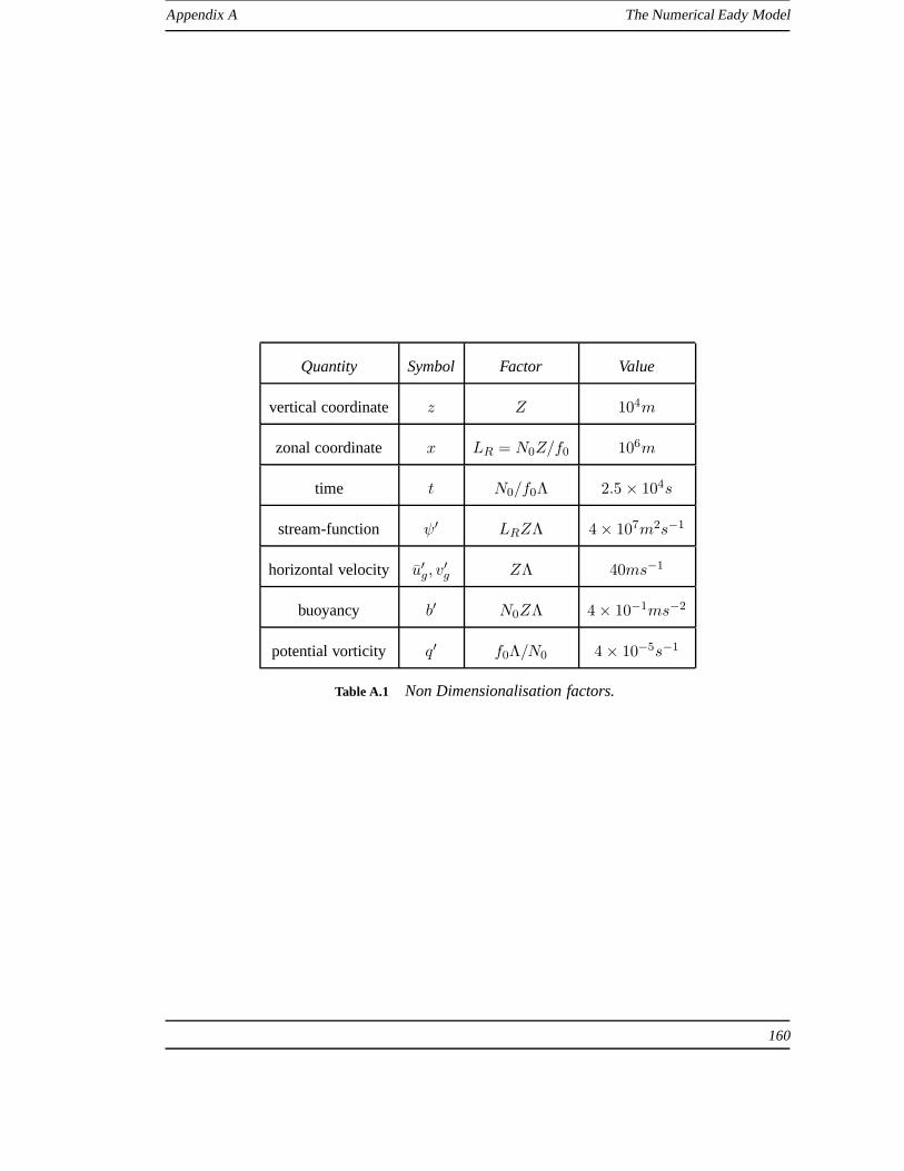
Appendix A The Numerical Eady Model
Quantity Symbol Factor Value
vertical coordinate z Z 104m
zonal coordinate x LR = N0Z/f0 106m
time t N0/f0Λ 2.5 × 10⁴s
stream-function ψ′ LRZΛ 4 × 10⁷m2s−1
horizontal velocity u′g, v′g ZΛ 40ms−1
buoyancy b′ N0ZΛ 4 × 10⁻¹ms−2
potential vorticity q′ f0Λ/N0 4 × 10⁻⁵s−1
Table A.1 Non Dimensionalisation factors.
160

APPENDIX B
Orthogonality between plane-waves
In this appendix we shall derive the condition for orthogonality between plane-waves of the same
zonal wavenumber. We shall start by defining two plane waves with the same zonal wavenumber
kn, but differing vertical wavenumbersm1 andm2. These two plane-waves are
ψ1 = cos (knx+m1z) , (B.1)
ψ2 = cos (knx+m2z) , (B.2)
wherem1 6= m2. Here it is worth reminding the reader that the tilt is related to the vertical
wavenumber bya = m/k. The two plane-waves are orthogonal if the integral of theirproduct
over the domain is equal to zero; i.e.
∫ X
0
∫ z2
z1
ψ1ψ2dzdx = 0. (B.3)
We shall start by rearranging the product
ψ1ψ2 = cos (knx+m1z) cos (knx+m2z) . (B.4)
Using the trigonometric identitycos(θ)cos(φ) = 12(cos(θ + φ) + cos(θ − φ)), we obtain
ψ1ψ2 =1
2cos (2knx+ [m1 +m2]z) + cos ([m1 −m2]z) . (B.5)
161

Appendix B Orthogonality between plane-waves
Using the further trigonometric identitycos(θ + φ) = cos(θ)cos(φ) − sin(θ)sin(φ), we obtain
ψ1ψ2 =1
2cos (2knx) cos ([m1 +m2]z) − sin (2knx) sin ([m1 +m2]z) + cos ([m1 −m2]z) .
(B.6)
Next we shall integrate the rearranged product with respectto x andz. Firstly we note that the
integral with respect tox of the wave termscos(2Knx) andsin(2knx) will vanish, since we are
integrating over whole periods of the wave. Integrating with respect tox and applying the limits
we obtain
∫ X
0
∫ z2
z1
ψ1ψ2dzdx =
∫ z2
z1
Xcos ([m1 −m2]z) dz. (B.7)
Integrating with respect toz we obtain
∫ X
0
∫ z2
z1
ψ1ψ2dzdx =
[
X
m1 −m2sin ([m1 −m2]z)
]z2
z1
. (B.8)
From this expression, it is evident thatψ1 andψ2 will be orthogonal ifsin ([m1 −m2]z1) =
sin ([m1 −m2]z2). This will occur for arbitraryz1 andz2 only if
(m1 −m2)z1 = (m1 −m2)z2 ± 2φπ, (B.9)
whereφ 6= 0 is an integer. Rearranging this condition and writing in terms of the tilta = m/kn,
we arrive at the condition that is imposed on the tilt to guarantee orthogonality between the plane
waves
δa = a1 − a2 =m1 −m2
kn
= ±2φπ
kn(z2 − z1). (B.10)
162

APPENDIX C
The relationship between a simple data assimilation systemand a
local projection operator
The aim of this appendix is to show that, if we neglect vertical correlations inB andR and
variations inB with zonal wavenumber and assuming the observations are colocated with model
height levels, then we may write
FQT (Rp +QpFTBFQT
p )−1QF T = FQTpDQpF
T , (C.1)
whereD is a diagonal matrix.Each diagonal element inD corresponds to an observation location
and is given
c(z) =r(z)
r(z) + b(z)(C.2)
wherer(z) andb(z) are diagonal elements ofR andB respectively andz is the height of the
observation.
To begin with we note that, in the absence of vertical correlations inR andB,Gp becomes block
diagonal with each invertible block,Gp, corresponding to a single vertical level. For this reason
we may treat each diagonal separately. If we assume that the observation error varies with height
only, then for a single block
R(z) = r(z)I, (C.3)
163

Appendix C Data assimilation and local projection
and likewise forB,
B(z) = b(z)I, (C.4)
We can define the inverse equation for a single block
(R(z) + QpFT B(z)F QT
p )−1 = (r(z)I + b(z)QpFT F QT
p )−1. (C.5)
For simplicity we shall drop the subscriptp for the rest of this appendix.
As in Bishop et al. (2001) we can make use of the fact that sinceit is symmetric, the eigenvectors
of QTFF TQ are form a complete orthonormal basis. We shall write the eigenvalue decomposi-
tion
QF TFQT = ΦΓΦT (C.6)
whereΓ is diagonal andΦ is orthonormal. SinceΦ is orthonormal, it satisfiesI = ΦΦT , therefore
we may write
(r(z)I + b(z)QF TFQT )−1 = (r(z)ΦΦT + b(z)ΦΓΦT )−1 = Φ(r(z)I + b(z)Γ)−1ΦT . (C.7)
We can also note that the eigenvectors and eigenvalues ofQT F F T Q are the right singular vec-
tors and singular values squared ofF T Q respectively. Assuming may define the singular value
decomposition ofF T Q as
F QT = ΩΥΦT , (C.8)
whereΩ is a matrix containing the left singular vectors andΥ is a possibly non-square diagonal
164

Appendix C Data assimilation and local projection
matrix that satisfiesΥTΥ = Γ. Using this singular value decomposition we may write
F QT Φ(r(z)I + b(z)Γ)−1ΦT QF T = ΩΥΦTΦ(r(z)I + b(z)Γ)−1ΦTΦΥT ΩT , (C.9)
and the fact thatΦTΦ = I we write
F QT Φ(r(z)I + b(z)Γ)−1ΦT QF T = ΩΥ(r(z)I + b(z)Γ)−1ΥT ΩT . (C.10)
Now we shall consider the form ofΥ(r(z)I + b(z)Γ)−1ΥT . The matrix(r(z)I + b(z)Γ)−1
is a diagonal matrix with theith diagonal element given by1/(r(z) + b(z)(Γ)i,i). It is worth
emphasising here that even if(Γ)i,i is zero, 1/(r(z) + b(z)(Γ)i,i) may not be. However,
(Υ(r(z)I + b(z)Γ)−1ΥT )i,i = (Γ)i,i/(r(z) + b(z)(Γ)i,i) and thereforeis equal to zero if
(Γ)i,i = 0. Furthermore if all the non-zero elements ofΓ have the same valueγ, we may write
F QTΦ(r(z)I + b(z)Γ)−1ΦT QF T = c(Q)ΩΥΥT ΩT , (C.11)
wherec(Q) = γ/(r(z) + γb(z)) is a scalar that depends on depends observation distribution Q.
Here it is worth noting that non-zero elements ofΓ will only have the same value for specific
choices ofQ. We shall discuss these choices ofQ a little further on. First however we note that,
from the definition of the singular value decomposition Equation (C.8)
c(Q)ΩΥΥT ΩT = c(Q)F QT QF T ≡ c(Q)T1(z), (C.12)
where T1(z) is a diagonal block of the local projection operatorT1 corresponding to a single
vertical level. For single a single observation on a vertical level and for an observation at ev-
ery grid-point on that level Equation (C.11) and ,consequently, Equation (C.12) are found to be
165

Appendix C Data assimilation and local projection
generally true. This result was obtained empirically, by comparing the matrices eigen-spectra of
(R+ QF TBFQ) andT1. This relationship was also found to hold exactly and approximately for
many cases, but for concision further discussion will be neglected.
166

APPENDIX D
Mathematical Symbols
AT : Transpose of general matrixA
A−1 : Inverse of general matrixA orA to the power−1
A+ : Psuedo-inverse of general matrixA
(A)i,j : ith, jth element of a general matrixA
(b)i : elementith of a general vectorb
Ai : Theith matrixA
bi : Theith vectorb
‖b‖2 = bT b : Vector 2-norm of general vectorb
‖b‖E = bTEb : Vector E-norm of general vectorb
I : Identity matrix
u : Left singular vector
U : Matrix of left singular vectors
v : Right singular vector
V : Matrix of right singular vectors
σ : Singular values
Σ : Matrix of singular values
167

Appendix D Mathematical Symbols
M : Non-linear numerical weather prediction model
M : Linear perturbation weather prediction model
χ : Weather forecast model state
δχ : Perturbation to weather forecast model state
J : Data assimilation cost function
H : Non-linear observation operator or foreward model
H : Linear observation operator or foreward model
R : Observation error covariance matrix
B : Background error covariance matrix
T : Local projection operator
E : E-Norm defining inner-product matrix
168

Appendix D Mathematical Symbols
x : Zonal spatial coordinate
y : Meridional spatial coordinate
z : Vertical spatial coordinate
t : Time
i : Zonally directed unit vector
j : Meridionally directed unit vector
k : Vertically directed unit vector
k : Zonal wavenumber
l : Meridional wavenumber
m : Vertical wavenumber
ψ : Quasi-geostrophic sreamfunction
q : Quasi-geostrophic potential vorticity
b : Scaled potential temperature perturbation (buoyancy)
u : Magnitude of zonal velocity
v : Magnitude of meridional velocity
w : Magnitude of vertical velocity
u = ui + vj + wk : Velocity
v = ui + vj : Horizontal velocity
f : Coriolis parameter
N : Static stability parameter
Λ : Eady model wind-shear parameter
X : Zonal extent of model domain
Z : Height of model domain
Ro : Rossby number
169
Bibliography
Badger, J., and B. J. Hoskins, 2001: Simple Initial Value Problems and Mechanisms for Baroclinic
Growth. J. Atmos. Sci., 58, 38–49.
Barkmeijer, J., M. Van Gijzen, and F. Bouttier, 1998: Singular vectors and estimates of the
analysis-error covariance metric.Quart. J. Roy. Meteor. Soc, 124(549), 1695–1713.
Bergot, T., 2001: Influence of the assimilation scheme on theefficiency of adaptive observations.
Quart. J. Roy. Meteor. Soc, 127, 635–660.
Bergot, T., G. Hello, A. Joly, and S. Malardel, May, 1999: Adaptive observations: a feasibility
study.Mon. Wea. Rev., 127, 743–765.
Berliner, L. M., Z. Q. Lu, and C. Snyder, August, 1999: Statistical design for adaptive weather
observations.J. Atmos. Sci., 56, 2536–2552.
Bishop, C. H., B. J. Etherton, and S. J. Majumbdar, March, 2001: Adaptive sampling with the
ensemble transform kalman filter. Part I: theoretical aspects. Mon. Wea. Rev., 129(3), 420–436.
Bishop, C. H., and A. J. Thorpe, 1994: Potential vorticity and the electrostatics analogy: Quasi-
geostrophic theory.Quart. J. Roy. Meteor. Soc, 120, 713–731.
Bishop, C. H., and Z. Toth, June, 1999: Ensemble transformation and adaptive observations.J.
Atmos. Sci., 56(11), 1748–1765.
170
References
Buizza, R., 1994: Localisation of optimal perturbations using a projection operator.Quart. J.
Roy. Meteor. Soc, 120, 1647–1682.
Buizza, R., 1997:The singular vector approach to the analysis of perturbation growth in the
atmosphere.PhD thesis, University College London.
Buizza, R., and A. Montani, 1999: Targeting Observations Using Singular Vectors.J. Atmos. Sci.,
56(17), 2965–2985.
Buizza, R., J. Tribbia, F. Molteni, and T. Palmer, 1993: Computation of optimal unstable struc-
tures for a numerical weather prediction model.Tellus, 45A(5), 388–407.
Chang, E. K. M., December, 1992: Resonating neutral modes ofthe Eady Model.J. Atmos. Sci.,
49(24), 2452–2463.
De Vries, H., and J. D. Opsteegh, 2005: Optimal perturbations in the eady model: resonance
versus PV unshielding.J. Atmos. Sci., 62, 492–505.
Eady, E. T., 1949: Long Waves and Cyclone Waves.Tellus, 1, 32–52.
Ehrendorfer, M., 2000: The total energy norm in a quasigeostrophic model. J. Atmos. Sci.,
57, 3443–3451.
Emanuel, K., D. Raymond, A. Betts, L. Bosart, C. Bretherton,K. Droegemeier, B. Farrell, J. M.
Fritsch, R. Houze, M. Lemone, D. Lilly, R. Rotunno, M. Shapiro, R. Smith, and A. Thorpe,
1995: Report on the first prospectus development team of the u.s. weather research-program to
NOAA and the NSF.Bull. Amer. Meteor. Soc., 76(7), 1194–1208.
Errico, R. M., T. Vukicevic, and K. Raeder, 1993: Examination of the accuracy of a tangent linear
model.Tellus, 45A, 462–477.
171
References
Farrell, B., 1984: Modal and non-modal baroclinic waves.J. Atmos. Sci., 41(4), 668–673.
Farrell, B., 1989: Optimal excitation of baroclinic waves.J. Atmos. Sci., 46(9), 1193–1206.
Farrell, B. F., October, 1990: Small error dynamics and the predictability of atmospheric flows.
J. Atmos. Sci., 47(20), 2409–2416.
Farrell, B.F., and P. J. Ioannou, 1996: Generalized stability theory. part I: Autonomous operators.
J. Atmos. Sci., 53(14), 2025–2040.
Fischer, C., 1998: Linear amplification and error growth in the 2d eady problem with uniform
potential vorticity.J. Atmos. Sci., 55, 3363–3380.
Frame, T., N. K. Nichols, and A. J. Thorpe, 2005: Structure and evolution of singular vectors in
the Eady model.Int. J. Numer. Meth. Fluids, 47, 1003–1009.
Gilmour, I., A. Leonard, and R. Buizza, 2001: Linear regime duration: Is 24 hours a long time in
synoptic weather forecasting.J. Atmos. Sci., 58(22), 3525–3539.
Golub, G. H., and C. F. Van Loan, 1983:Matrix Computations. John Hopkins University Press.
Green, J. S. A., 1960: A problem in baroclinic stability.Quart. J. Roy. Meteor. Soc, 86, 237–251.
Hamill, T. H., and C. Snyder, 2002: Using improved background-error covariances from an En-
semble Kalman Filter for adaptive observations.Mon. Wea. Rev., 130, 1552–1572.
Hamill, T. M., and C. Snyder, 2002: Analysis-error statistics of a quasigeostrophic model using
three-dimensional variational assimilation.Mon. Wea. Rev., 130, 2777–2790.
Holton, J. R., 1992:An introduction to dynamic meteorology, third ed. Academic Press.
172

References
Hoskins, B. J., R. Buizza, and J. Badger, 2000: The nature of singular vector growth and structure.
Quart. J. Roy. Meteor. Soc, 126, 1565–1580.
Hoskins, B. J., M. E. Mcintyre, and A.W. Robertson, 1985: On the use and significance of isen-
tropic potential vorticity maps.Quart. J. Roy. Meteor. Soc, 111(470), 877–946.
Kim, Hyun Mee, and Michael C. Morgan, 2002: Dependence of sigular vector structure and
evolution on the choice of norm.J. Atmos. Sci., 59, 3099–3116.
Kim, Hyun Mee, Michael C. Morgan, and Rebecca E. Morss, 2004:Evolution of analysis error
and adjoint-based sensitivities: Implications for adaptive observations.J. Atmos. Sci., 61, 795–
812.
Leutbecher, M., March, 2003: A reduced rank estimate of forecast error variance changes due to
intermittent modifications of the observation network.J. Atmos. Sci., 742(5), 729.
Leutbecher, M., J. Barkmeijer, T. N. Palmer, and A. J. Thorpe, 2002: Potential improvement
to forecasts of two severe storms using targeted observations. Quart. J. Roy. Meteor. Soc,
128, 1641–1670.
LI, Zhi Jin, I. M. Navon, and M. Y. Hussaini, 2005: Analysis ofthe singular vectors of the full-
physics florida state university global spectral model.Tellus, 57(4), 560–574.
Lorenz, E. N., March, 1963: Determinisitc nonperiodic flow.J. Atmos. Sci., 20, 130–141.
Lorenz, E. N., 1965: A study of the predictability of a 28-variable atmospheric model.Tellus,
17(3), 321–333.
Lorenz, E. N., and K. E. Emanuel, 1998: Optimal sites for supplementary observations: Simula-
tions with a small model.J. Atmos. Sci., 55, 399–414.
173
References
Majumdar, S. J., C. H. Bishop, and B. J. Etherton, May, 2002: Adaptive sampling with the
Ensemble Transform Kalman Filter. Part II field program implementation. Mon. Wea. Rev.,
130, 1356–1369.
Majumdar, S. J., C. H. Bishop, B. J. Etherton, I. Szunyogh, and Z. Toth, October, 2001: Can an
ensemble transform kalman filter predict the reduction in forecast-error variance produced by
targeted observations?Quart. J. Roy. Meteor. Soc, 127(578), 2803–2820.
Molteni, F., , R. Buizza, T. N. Palmer, and T. Petroliagis, 1996: The new ECMWF ensemble
prediction system: methodology and validation.Quart. J. Roy. Meteor. Soc, 119(47), 73–119.
Montani, A., 1998:Targeting of observations to improve forecasts of cyclogenisis. PhD thesis,
Dept. of Meteorology, University of Reading.
Montani, A., and A. J. Thorpe, 2002: Mechanisms leading to singular-vector growth for FASTEX
cyclones.Quart. J. Roy. Meteor. Soc, 128(579), 131–148.
Morgan, M. C., September, 2001: A potential vorticity and wave activity diagnosis of optimal
perturbation evolution.J. Atmos. Sci., 58, 2518–2544.
Morgan, M. C., and C. C. Chen, January, 2002: Diagnosis of optimal perturbation evolution in
the eady model.J. Atmos. Sci., 59(2), 169–185.
Morss, R. E., K. A. Emanuel, and C. Snyder, January, 2001: Idealised adaptive observation strate-
gies for improving numerical weather prediction.J. Atmos. Sci., 58, 210–232.
Mukougawa, H., and T. Ikeda, 1994: Optimal excitation of baroclinic waves in the eady model.
J. Meteor. Soc. Japan, 72(4), 499–513.
174

References
Orr, W. McF., 1907: Stability or instability of the steady-motions of a perfect liquid.Proc. Roy.
Irish Acad., 27, 9–69.
Palmer, T. N., R. Gelaro, J. Barkmeijer, and R. Buizza, 1998:Singular Vectors, Metrics and
Adaptive observations.J. Atmos. Sci., 55, 633–653.
Pedlosky, J., 1964: An initial value problem in the theory ofbaroclinic instability. Tellus,
16(1), 12–17.
Pedlosky, J., 1979:Geophysical fluid dynamics, second ed. springer.
Pu, Z. X., E. Kalnay, J. Sela, and I. Szunyogh, 1997: Sensitivity of forecast errors to intial condi-
tions with a quasi-inverse linear method.Mon. Wea. Rev., 125, 2479–2503.
Pu, Z. X., S. J. Lord, and E. Kalnay, 1998: Forecast sensitivity with dropwindsonde data and
targeted observations.Tellus, 50A, 391–410.
Rabier, F., and P. Courtier, 1992: Four-dimensional assimilation in the presence of baroclinic
instability. Quart. J. Roy. Meteor. Soc, 118, 649–672.
Snyder, C., T. M. Hamill, and S. B. Trier, 2003: Linear evolution of error covariances in a
quasiqeostrophic model.Mon. Wea. Rev., 131, 189–205.
Strang, 1988:Linear Algebra and its Applications. Brooks, Cole.
Thompson, P. D., 1957: Uncertainty of initial state as a factor in the predictability of large scale
atmospheric flow patterns.Tellus, 9(3), 275–295.
Thorncroft, C. D., and B. J. Hoskins, October, 1990: Frontalcyclogenesis. J. Atmos. Sci.,
47(19), 2317–2336.
175

References
Toth, Z, and E Kalnay, 1997: Ensemble forecasting at ncep andthe breeding method.Mon. Wea.
Rev., 125(12), 3297–3319.
Vukicevic, T, 1991: Non-linear and linear evolution of initial forecast errors.Mon. Wea. Rev.,
199, 1602–1611.
176