Embed Size (px)
Citation preview

Methods For Analysis Of Passenger Trip Performance In A Complex NetworkedTransportation System
A dissertation submitted in partial fulfillment of the requirements for the degree ofDoctor of Philosophy at George Mason University
By
Danyi WangBachelor of Science
Wuhan University of Technology, 2000Master of Science
George Mason University, 2002
Director: Dr. Lance Sherry, Associate ProfessorDepartment of Systems Engineering and Operations Research
Summer Semester 2007George Mason University
Fairfax, VA

ii
Copyright c© 2007 by Danyi WangAll Rights Reserved

iii
Acknowledgments
My sincerest gratitude goes to Dr. Lance Sherry and Dr. George Donohue. Withouttheir encouragement and trust, none of this research would have been accomplished.
First I wish to thank Dr. Lance Sherry, who guided this work and helped when-ever I was in need. His work ethics and professional qualities are a great source ofinspiration for me, and will stay as such in my future endeavors. His presence at theCATSR was the best thing that could happen to me and my thesis. Dr. Lance Sherrytruly was always a caring mentor and understanding advisor. I am deeply gratefulfor the effort he put into my education and the full, unceasing confidence he has inme. I am indebted to him more than he knows.
Similarly, I am extremely grateful to Dr. George Donohue, who taught me in-valuable and enduring lessons during my stay at GMU. Beyond his broad knowledge,outstanding vision and academic virtues, I am also grateful for the many discussionswith him that taught me the values of integrity and persistence. I still rememberthe talk between him and me in the coffee shop at Johnson Center. I was deeplytouched by his enthusiasm to work and positive attitude toward obstacle. Thank youDr. Donohue, for your sharing and caring, and for all you have done to help andencourage me.
It is a pleasure for me to have Dr. Andrew Sage, Dr. John Shortle and Dr.Abbas Zaidi on my committee as well. I deeply appreciate their insightful sugges-tions, generous help and warm encouragements throughout the completion of thisdissertation.
Finally, I take this opportunity to express my profound appreciation to my belovedparents and my husband Tao. Their endless love, great patience, and consistentsupport held me through to the end.

iv
Table of Contents
Page
List of Abbreviations . . . . . . . . . . . . . . . . . . . . . . . . . . . . . . . . xi
Abstract . . . . . . . . . . . . . . . . . . . . . . . . . . . . . . . . . . . . . . . xii
1 Introduction . . . . . . . . . . . . . . . . . . . . . . . . . . . . . . . . . . 1
1.1 Correlation between Traffic Growth and Flight On-Time Performance 2
1.2 Correlation between Flight On-Time Performance and Passenger On-
Time Performance . . . . . . . . . . . . . . . . . . . . . . . . . . . . 7
1.3 Problem Statement . . . . . . . . . . . . . . . . . . . . . . . . . . . . 12
1.3.1 Research Objectives . . . . . . . . . . . . . . . . . . . . . . . 13
1.3.2 Research Approach . . . . . . . . . . . . . . . . . . . . . . . . 13
1.4 Contributions . . . . . . . . . . . . . . . . . . . . . . . . . . . . . . . 14
1.4.1 Industrial Applications of Research . . . . . . . . . . . . . . . 15
1.4.2 Papers . . . . . . . . . . . . . . . . . . . . . . . . . . . . . . . 16
2 Literature Review . . . . . . . . . . . . . . . . . . . . . . . . . . . . . . . 18
2.1 Flight On-Time Performance Measurement . . . . . . . . . . . . . . . 18
2.2 Passenger On-Time Performance Measurement . . . . . . . . . . . . . 21
2.3 Petri Nets and Applications in Transportation Systems . . . . . . . . 27
2.3.1 Introduction of Petri Nets . . . . . . . . . . . . . . . . . . . . 27
2.3.2 Petri Net Application in Transportation Systems . . . . . . . 32
3 EPTD Algorithms and Database (Methods and Results) . . . . . . . . . . 35
3.1 Flight DataBases . . . . . . . . . . . . . . . . . . . . . . . . . . . . . 38
3.1.1 Airline On-Time Performance Database . . . . . . . . . . . . . 38
3.1.2 Air Carrier Statistics (T-100) Database . . . . . . . . . . . . . 41
3.1.3 Airline Origin and Destination Survey (DB1B) Market Database 43
3.2 Algorithms . . . . . . . . . . . . . . . . . . . . . . . . . . . . . . . . . 45
3.2.1 Data Processing Algorithm . . . . . . . . . . . . . . . . . . . . 45
3.2.2 Data Joining Algorithm . . . . . . . . . . . . . . . . . . . . . 46

v
3.2.3 Estimating Passenger Trip Delay (EPTD) Algorithm . . . . . 48
3.3 Analysis and Results . . . . . . . . . . . . . . . . . . . . . . . . . . . 55
3.3.1 Disproportionately High EPTD Generated By Cancelled Flights 55
3.3.2 EPTD Trend Analysis (2000-2006) . . . . . . . . . . . . . . . 57
3.3.3 Asymmetric Performance of EPTD . . . . . . . . . . . . . . . 61
3.3.4 Heavily Skewed Distribution of EPTD . . . . . . . . . . . . . 67
3.3.5 ATNAT Tool . . . . . . . . . . . . . . . . . . . . . . . . . . . 79
3.4 Validation . . . . . . . . . . . . . . . . . . . . . . . . . . . . . . . . . 85
4 Passenger Flow Simulation (Methods and Results) . . . . . . . . . . . . . 86
4.1 The Underlying Concept . . . . . . . . . . . . . . . . . . . . . . . . . 87
4.2 Petri Net Modeling Tool . . . . . . . . . . . . . . . . . . . . . . . . . 88
4.3 Structure of Passenger Flow Simulation (PFS) . . . . . . . . . . . . . 89
4.3.1 PFS Overview . . . . . . . . . . . . . . . . . . . . . . . . . . . 90
4.3.2 PFS Color Definition . . . . . . . . . . . . . . . . . . . . . . . 90
4.3.3 PFS Declaration . . . . . . . . . . . . . . . . . . . . . . . . . 92
4.3.4 PFS Hierarchy . . . . . . . . . . . . . . . . . . . . . . . . . . 92
4.3.5 PFS Top Level Net . . . . . . . . . . . . . . . . . . . . . . . . 93
4.3.6 PFS En route Subnet (2nd Level) . . . . . . . . . . . . . . . . 95
4.3.7 PFS Airport Subnet (2nd Level) . . . . . . . . . . . . . . . . . 98
4.3.8 PFS Passenger Loading Subnet(3rd Level) . . . . . . . . . . . 104
4.3.9 Passenger Missed Connection Algorithm in PFS . . . . . . . . 107
4.4 Deterministic Passenger Flow Simulation (PFS) . . . . . . . . . . . . 110
4.4.1 Simulation Results and Validation: 34-Airport PFS on July 6
2005 . . . . . . . . . . . . . . . . . . . . . . . . . . . . . . . . 110
4.4.2 Design of Experiment (DOE) . . . . . . . . . . . . . . . . . . 113
4.4.3 Rank Order Significant Factors . . . . . . . . . . . . . . . . . 116
4.4.4 Sensitivity of Factors . . . . . . . . . . . . . . . . . . . . . . . 123
4.5 Stochastic Passenger Flow Simulation (PFS) . . . . . . . . . . . . . . 124
4.5.1 Stochastic Factors and Variables . . . . . . . . . . . . . . . . . 125
4.5.2 Simulation Results and Validation: 34-Airport PFS on July 6
2005 . . . . . . . . . . . . . . . . . . . . . . . . . . . . . . . . 127
5 Industrial Applications of Research . . . . . . . . . . . . . . . . . . . . . . 131
5.1 Traffic Flow Management (Fall 2006) . . . . . . . . . . . . . . . . . . 132

vi
5.2 FAA NAS Strategy Simulator (Spring 2007) . . . . . . . . . . . . . . 134
5.2.1 EPTD in 2010 . . . . . . . . . . . . . . . . . . . . . . . . . . . 135
5.2.2 EPTD Module for NSS . . . . . . . . . . . . . . . . . . . . . . 141
6 Conclusions and Future Work . . . . . . . . . . . . . . . . . . . . . . . . . 144
6.1 Disproportionately High EPTD due to Cancelled Flights and Missed
Connections . . . . . . . . . . . . . . . . . . . . . . . . . . . . . . . . 144
6.2 Asymmetric Behavior of EPTD in terms of Routes, Airports and Months
145
6.3 Flight-Based and Passenger-Based Metrics . . . . . . . . . . . . . . . 145
6.4 Accuracy of EPTD . . . . . . . . . . . . . . . . . . . . . . . . . . . . 146
6.5 Dealing with the Cancelled Flight Phenomenon . . . . . . . . . . . . 147
6.6 Passenger Perspective . . . . . . . . . . . . . . . . . . . . . . . . . . . 148
6.7 Consumer Protection for Airline Travelers . . . . . . . . . . . . . . . 149
6.8 Recommendations for Future Work . . . . . . . . . . . . . . . . . . . 149
Bibliography . . . . . . . . . . . . . . . . . . . . . . . . . . . . . . . . . . . . . 152
A Appendix A . . . . . . . . . . . . . . . . . . . . . . . . . . . . . . . . . . . 161
A.1 Airline On-Time Performance (AOTP) Database . . . . . . . . . . . 161
A.2 Air Carrier Statistics (T-100) Database . . . . . . . . . . . . . . . . . 166
A.3 Airline Origin and Destination Survey (DB1B) Market Database . . . 171
B Appendix B . . . . . . . . . . . . . . . . . . . . . . . . . . . . . . . . . . . 175
C Appendix C . . . . . . . . . . . . . . . . . . . . . . . . . . . . . . . . . . . 177
D Appendix D . . . . . . . . . . . . . . . . . . . . . . . . . . . . . . . . . . . 191
E Appendix E . . . . . . . . . . . . . . . . . . . . . . . . . . . . . . . . . . . 267

vii
List of Tables
Table Page
1.1 Passenger Trip Delay due to Cancelled Flights on Route ORD-LGA . 10
1.2 Distinction Between The Vehicle Tier And The Passenger Tier . . . . 11
2.1 Differences Between Passenger Trip Delay Estimation Models . . . . . 26
3.1 Airline On-Time Performance Release History . . . . . . . . . . . . . 39
3.2 Data Processing Algorithm . . . . . . . . . . . . . . . . . . . . . . . . 45
3.3 Data Joining Algorithm . . . . . . . . . . . . . . . . . . . . . . . . . 48
3.4 Comparison of Statistics for Distribution of Flight Delays and Distribution
of Passenger Trip Delays . . . . . . . . . . . . . . . . . . . . . . . . . . 75
3.5 Example of Using 15-POTP for Purchasing Airline Tickets . . . . . . 78
3.6 Airports and Airlines Included in the ATNAT Tool . . . . . . . . . . 80
4.1 Overview of Passenger Flow Simulation Model . . . . . . . . . . . . . 90
4.2 Validation of Deterministic PFS . . . . . . . . . . . . . . . . . . . . . 112
4.3 Initial Significant Factors and Their Categories . . . . . . . . . . . . . 114
4.4 High and Low Level Settings for Factors . . . . . . . . . . . . . . . . 115
4.5 Sensitivity of the Total EPTD (Delay+Cancel+Missed-Connection) to
Changes in Factors . . . . . . . . . . . . . . . . . . . . . . . . . . . . 124
4.6 Stochastic Simulation Results of the Stochastic PFS on July 6, 2005 . 128
4.7 Validation of Stochastic PFS . . . . . . . . . . . . . . . . . . . . . . . 129
5.1 Comparison Between Average Daily Performance in 2005 and 2010 . 140
5.2 Comparison Between Average Daily Performance in 2000 and 2010 . 140

viii
List of Figures
Figure Page
1.1 Screen Shot of BTS On-Time Performance Statistics in 2000, Source:BTS 3
1.2 Flight On-Time Percentage, 1990-2007, Data Source:BTS . . . . . . . . . 5
1.3 Growth of Enplanements and Revenue Passenger Miles (RPMs), 1978-2006,
Source:ATA . . . . . . . . . . . . . . . . . . . . . . . . . . . . . . . . 5
1.4 Historical Load Factor from 1978 to 2006, Source:ATA . . . . . . . . . . 6
1.5 Vehicle Tier and Passenger Tier of Air Transportation System . . . . . . 8
2.1 Passenger Trip Delay Statistics, Source: Stephane Bratu’s Thesis, 2003, MIT 23
2.2 Decision Tree to Determine Passenger Disruption Probability, Source: Uni-
versity of Maryland . . . . . . . . . . . . . . . . . . . . . . . . . . . . . 24
2.3 Firing of a Transition, Source: (Perdu, 1997), (Wagenhals, 2000) . . . . . 28
2.4 Firing of a Transition in Timed Colored Petri Nets, Source: (Perdu, 1997) 31
2.5 Simulate Passenger Flow in the Public Bus Transportation System, Source:
(Castelain and Mesghouni, 2002) . . . . . . . . . . . . . . . . . . . . . . 34
3.1 Overview of Methods and Model . . . . . . . . . . . . . . . . . . . . . . 37
3.2 Airline On-Time Performance Database Description and Definitions . . . . 40
3.3 Air Carrier Statistics (T-100) Database Description and Definitions . . . . 41
3.4 Sample: Air Carrier Statistics (T-100) database . . . . . . . . . . . . . . 42
3.5 Airline Origin and Destination Survey (DB1B) Market Database Descrip-
tion and Definitions . . . . . . . . . . . . . . . . . . . . . . . . . . . . 43
3.6 Sample: Airline Origin and Destination Survey (DB1B) Market Database . 44
3.7 Data Join Algorithm . . . . . . . . . . . . . . . . . . . . . . . . . . . . 47
3.8 Example of Estimating Passenger Delays Due to Cancelled Flights . . . . 52
3.9 Estimating Passenger Trip Delay Algorithm . . . . . . . . . . . . . . . . 53
3.10 Total Estimated Passenger Trip Delay in Year 2006 . . . . . . . . . . . . 56
3.11 Annual Total Scheduled Flights and Enplanements from Year 2000 to Year
2006) . . . . . . . . . . . . . . . . . . . . . . . . . . . . . . . . . . . . 58

ix
3.12 Trend Analysis for Total Estimated Passenger Trip Delay (2000 2̃006) . . 59
3.13 Trend Analysis for Average Estimated Passenger Trip Delay (2000 2̃006) . 60
3.14 EPTD by Month: Five months of the year account for 51% of the EPTD in
2006 . . . . . . . . . . . . . . . . . . . . . . . . . . . . . . . . . . . . 61
3.15 # of Cancellations by Month: Four months of the year account for 50% of
EPTD due to cancelled flights in 2006 . . . . . . . . . . . . . . . . . . . 62
3.16 EPTD by Route: Fifty Percent of the Annual EPTD is Generated by 17%
of the 1030 Routes between OEP-35 airports . . . . . . . . . . . . . . . 64
3.17 Histogram for Average EPTD by Route in 2006 . . . . . . . . . . . . . . 65
3.18 EPTD by Airport (Destination): Fifty Percent of the Annual EPTD is
Generated by the Top 9 OEP-35 Airports . . . . . . . . . . . . . . . . . 66
3.19 Histogram for Average EPTD by Airport in 2006 . . . . . . . . . . . . . 67
3.20 Right-tailed distribution of flight (or passenger) delays. Identifies 3 pairs of
parameters used in this paper to characterize the distribution. Distribution
for passenger trip delay has similar form with longer right-tail. . . . . . . 68
3.21 Sample Statistics for Flight Delays and Passenger Trip Delays Statistics . 71
3.22 Histograms of Flight Percentage of On-Time and Passenger Percentage of
On-Time (15-OTP v.s. 15-POTP) . . . . . . . . . . . . . . . . . . . . . 72
3.23 Histograms of Average Magnitude of Flight Delays and Average Magnitude
of Passenger Trip Delays . . . . . . . . . . . . . . . . . . . . . . . . . . 73
3.24 Histograms of Average Worst-Case Magnitude of Flight Delays and Average
Worst-Case Magnitude of Passenger Trip Delays . . . . . . . . . . . . . . 74
3.25 Plots of Reliability of Routes Between Washington D.C. and Chicago . . . 78
3.26 The Air Transportation Network Analysis Tool (ATNAT) . . . . . . . . . 81
3.27 Combinations of Inputs and Outputs for ATNAT . . . . . . . . . . . . . 81
3.28 Statistic Parts of GUI for Routes DFW-ATL and MSP-ORD . . . . . . . 83
3.29 Graphic Parts of GUI for Routes DFW-ATL and MSP-ORD . . . . . . . 84
4.1 Underlying Concepts for Passenger Flow Simulation Model . . . . . . . . 87
4.2 Example: Passenger Boarding Process . . . . . . . . . . . . . . . . . . . 91
4.3 Three-Level Hierarchy of Passenger Flow Simulation Model . . . . . . . . 93
4.4 Top Level Page for 34-Airport PFS . . . . . . . . . . . . . . . . . . . . 94
4.5 Enroute Subnet for a Single Route (ATL-LGA) for 4-Airport PFS . . . . 95
4.6 Enroute Subnet for 34-Airport PFS . . . . . . . . . . . . . . . . . . . . 97
4.7 Airport Subnet (ORD) for 4-Airport PFS . . . . . . . . . . . . . . . . . 99

x
4.8 Step 1: Splitting PaxGroup at ORD airport . . . . . . . . . . . . . . . . 100
4.9 Step 2: Re-clustering PaxGroup at ORD airport . . . . . . . . . . . . . . 101
4.10 Step 3: Loading PaxDelay at ORD airport . . . . . . . . . . . . . . . . . 103
4.11 Passenger Loading Subnet for Route ORD-ATL . . . . . . . . . . . . . . 106
4.12 Example of Purchasing Air Ticket Online . . . . . . . . . . . . . . . . . 108
4.13 Estimate Passenger Trip Delay in PFS . . . . . . . . . . . . . . . . . . . 109
4.14 Deterministic PFS Simulation Results for July 6 2005 . . . . . . . . . . . 111
4.15 Coefficient Plot for NAS-Wide Total EPTD . . . . . . . . . . . . . . . . 117
4.16 Coefficient Plot for Total EPTD due to Cancelled Flights . . . . . . . . . 119
4.17 Coefficient Plot for Total EPTD due to Miss-Connections . . . . . . . . . 120
4.18 Coefficient Plot for Average EPTD due to Miss-Connections . . . . . . . 122
4.19 Coefficient Plot for Average EPTD due to Delayed Flights . . . . . . . . 123
5.1 Example of GDP in Support of SWAP (?) . . . . . . . . . . . . . . . . . 133
5.2 Load Factor from 1978 to 2006, Data Source: ATA . . . . . . . . . . . . 136
5.3 Percentage of Delayed Flights from 2002 to 2007 , Data Source: BTS . . . 136
5.4 Correlations Between Percentage of Delayed Flights and Percentage of Can-
celled Flights, Data Source: BTS . . . . . . . . . . . . . . . . . . . . . . 137
5.5 Estimation Passenger Trip delay in 2010 . . . . . . . . . . . . . . . . . . 138
5.6 Estimating Passenger Trip Delay Module for NSS . . . . . . . . . . . . . 142
5.7 Equations Used in the NSS Module . . . . . . . . . . . . . . . . . . . . 143
A.1 Data Release History for AOTP . . . . . . . . . . . . . . . . . . . . . . 162
A.2 Database Description and Definitions for AOTP . . . . . . . . . . . . . . 163
A.3 Data Field Names and Descriptions for AOTP . . . . . . . . . . . . . . . 164
A.4 Field Names and Descriptions for AOTP (Cont) . . . . . . . . . . . . . . 165
A.5 Data Release History for T-100 (first 32 of 174 carriers) . . . . . . . . . . 167
A.6 Database Description and Definitions for T-100 . . . . . . . . . . . . . . 168
A.7 Field Names and Descriptions for T-100 . . . . . . . . . . . . . . . . . . 169
A.8 Field Names and Descriptions for T-100 (Cont) . . . . . . . . . . . . . . 170
A.9 Data Release History for T-100 . . . . . . . . . . . . . . . . . . . . . . 171
A.10 Data Release History for T-100 (Cont) . . . . . . . . . . . . . . . . . . . 172
A.11 Database Description and Definitions for T-100 . . . . . . . . . . . . . . 173
A.12 Field Names and Descriptions for T-100 . . . . . . . . . . . . . . . . . . 174
B.1 Operational Evolution Plan (OEP) 35 Airports . . . . . . . . . . . . . . 176

xi
LIST OF ABBREVIATIONS
AOTP Airline On-Time Performance Database ASPM Aviation System Performance Metrics ASQP Airline Service Quality Performance ASM Available Seat Mile ATNAT Air Transportation Network Analysis Tool ATA Air Transportation Association ATS Air Transportation System BTS Bureau of Transportation Statistics CPN Color Petri Net DOT Department of Transportation ENP Enplanement EPTD Estimated Passenger Trip Delay FAA Federal Aviation Administration GUI Graphic User Interface MCT Minimal Connecting Time NAS National Airspace System NASA National Aeronautics and Space Administration NEXTOR The National Center of Excellence for Aviation Operations Research NSS NAS Strategy Simulator OAG O cal Airline Guide OEP Operational Evolution Plan PAX Passenger PAXDELAY Passenger Trip Delay PAXGROUP Passenger Group PFS Passenger Flow Simulation RPM Revenue Passenger Miles TRB Transportation Research Board

Abstract
METHODS FOR ANALYSIS OF PASSENGER TRIP PERFORMANCE IN A COM-PLEX NETWORKED TRANSPORTATION SYSTEM
Danyi Wang, PhD
George Mason University, 2007
Dissertation Director: Dr. Lance Sherry
The purpose of the Air Transportation System (ATS) is to provide safe and ef-
ficient transportation service of passengers and cargo. The on-time performance of
a passenger’s trip is a critical performance measurement of the Quality of Service
(QOS) provided by any Air Transportation System. QOS has been correlated with
airline profitability, productivity, customer loyalty and customer satisfaction (Heskett
et al. 1994).
Btatu and Barnhart have shown that official government and airline on-time per-
formance metrics (i.e. flight-centric measures of air transportation) fail to accurately
reflect the passenger experience (Bratu and Barnhart, 2005). Flight-based metrics
do not include the trip delays accrued by passengers who were re-booked due to can-
celled flights or missed connections. Also, flight-based metrics do not quantify the
magnitude of the delay (only the likelihood) and thus fails to provide the consumer
with a useful assessment of the impact of a delay. Passenger-centric metrics have
not been developed because of the unavailability of airline proprietary data, which is
also protected by anti-trust collusion concerns and civil liberty privacy restrictions.

xiii
Moveover, the growth of the ATS is trending out of the historical range.
The objectives of this research were to (1) estimate ATS-wide passenger trip delay
using publicly accessible flight data, and (2) investigate passenger trip dynamics out
of the range of historical data by building a passenger flow simulation model to
predict impact on passenger trip time given anticipated changes in the future. The
first objective enables researchers to conduct historical analysis on passenger on-time
performance without proprietary itinerary data, and the second objective enables
researchers to conduct experiments outside the range of historic data.
The estimated passenger trip delay was for 1,030 routes between the 35 busiest
airports in the United States in 2006. The major findings of this research are listed
as follows:
1. High passenger trip delays are disproportionately generated by cancelled flights and
missed connections. Passengers scheduled on cancelled flights or missed connections
represent 3 percent of total enplanements, but generated 45 percent of total passenger
trip delay. On average, passengers scheduled on cancelled flights experienced 607
minutes delay, and passengers who missed the connections experienced 341 minutes
delay in 2006. The heavily skewed distribution of passenger trip delay reveals the
fact that a small proportion of passengers experience heavy delays, which can not be
reflected by flight-based performance metrics.
2. Trend analysis for passenger trip delays from 2000 to 2006 shows the increase in flight
operations slowed down and leveled off in 2006, while enplanements kept increasing.
This is due to the continuous increase in load factor. Load factor has increased from
69% in 2003 to 80% in 2006. Passenger performance is very sensitive to changes in
flight operations: annual total passenger trip delay was increased by 17% and 7%
from 2004 to 2005, and from 2005 to 2006, while flight operations barely increased
(0.5% from 2004 to 2005, and no increase from 2005 to 2006) during the same time
period.

xiv
3. Passenger trip delay is shown to have an asymmetric performance of passenger trip
delay in terms of routes. Seventeen percent of the 1030 routes generated 50 percent
of total passenger trip delays. An interesting observation is that routes between the
New York metropolitan area and the Washington D.C. metropolitan area have the
highest average passenger trip delays in the system.
4. In terms of airports, there is also an asymmetric performance of passenger trip delay.
Nine of the 35 busiest airports generated 50 percent of total passenger trip delays.
Some airports, especially major hubs, impact the passenger trip delays significantly
more than others. Recognition of this asymmetric performance can help reduce the
total passenger trip delay propagation in the air transportation network by making
changes primarily in major airports, such as Atlanta, GA (ATL), Chicago O’Hare
(ORD) and Newark (EWR) airports.
5. Congestion Flight Delay, Load Factor, Flight Cancellation Time, and Airline Cooper-
ation Policy are the most significant factors affecting total passenger trip delay in the
system. A 15-minute reduction in flight delay is predicted to produce a 24 percent
decrease in total passenger trip delays, and should save approximately $2.3 million in
passenger value of time per day. An improved airline cooperation policy in re-booking
disrupted passengers is predicted to produce a 12 percent decrease in total passenger
trip delays, and flights cancelled earlier in the day is predicted to produce a 10 percent
decrease in total passenger trip delay. The load factor has increased from 70 percent
in 2000 to 80 percent in 2006. The systemically high load factors lead to a very brit-
tle transportation system that has little resiliency or adaptability when confronted
with either weather or congestion induced flight cancellations (Donohue and Shaver,
2008). Decreasing the load factor to 70 percent is predicted to produce an 8 percent
reduce in total passenger trip delay. The combined effect of multiple factors should
be investigated and used to support the decisions made by officials, policy makers
and researchers, so that they can achieve their strategy goals with minimal costs or
changes associated with the most significant factors.

xv
This dissertation provides new system performance measurements from the pas-
senger’s view. The results of this research provides decision makers with improved
metrics for future investment decisions and better tools to manage the system. The
passenger flow simulation model also provide the means to perform analysis for pro-
posed changes to the system.
Chapter 1: Introduction
According to Air Transportation Association (ATA) statistics, U.S. passenger and
cargo airlines recorded $163 billion operational revenue in 2006. Although flight
schedule and ticket prices have proven to be the main drivers of airline profitability,
studies show that ontime performance and service reliability are important to achiev-
ing long-term profitability (Bratu, 2003) Customer satisfaction is a key player in
the service-profit chain, which drives airline profitability, productivity and customer
loyalty and satisfaction (Heskett et al., 1994).
Except for slot constrained airports, airlines are able to schedule as many flights as
they wish at all airports. Data recently released by the U.S. Air Transportation Asso-
ciation (ATA) show that passenger enplanements, revenue passenger miles (RPMs),
available seat miles (ASMs), passenger load factor (LF) and cargo revenue ton miles
(RTMs) for U.S. carriers reached new highs in 2006. U.S. airline operations grew to
11.3 million departures, with carriers transporting 745 million passengers and 797 bil-
lion RPMs systemwide. “Higher volumes of traffic, which are expected to continue to
grow, strongly reinforce the need to modernize our antiquated air traffic control sys-
tem,” said Air Transportation Association (ATA) Vice President and Chief Economist
John Heimlich. “It is imperative that we implement technology upgrades and adopt
procedures that will accommodate the growing demand being placed on the system by
all users of ATC services and infrastructure. Without an effective transformation of
the ATC system, the negative impact on our nation’s economy will be severe.” (ATA
1

2
news release May 1, 2006) Moreover, the disproportionate increase in flights relative
to total airport capacity resulted in severe system congestion, and numerous flight
delays and cancellations, adversely affecting the traveling public (Tam and Hansman,
2003),(Bratu, 2003).
1.1 Correlation between Traffic Growth and Flight
On-Time Performance
The economic boom in the mid to late 1990s stimulated the growth in air travel
demand. Traffic loads and profits for the airline industry during this period set new
records. In the 2000, the U.S. airline industry operated in excess of 23,000 domestic
and international flights per day, and enplaned more than 1.7 million daily passengers,
more than 85 percent of whom have a choice of two or more airlines. The industry
added nearly 300 billion dollars into our national economy in 2000 (ATA Report).
Between 1990 and 2000, the domestic revenue passenger miles at the major US
carriers increased by 40 percent, while total aircraft seat capacity increased by only
23 percent. Load factors climbed to record levels: the average load factor in 1990 was
60 percent, but that had increased to 70 percent by 2000 (Tam and Hansman, 2003).
In conjunction with the high load factor, airport runway capacity/flight demand
imbalance drove flight on-time percentage from 82 percent in the early 90’s down
to 73 percent in 2000. Detailed flight on-time performance in 2000 is described in
Figure 1.1. The percentage of delayed flights and cancelled flights were as high as 30
percent in June 2000 and 6 percent in December 2000, respectively, while the values
of these two metrics were only 19 percent and 1 percent in 1990.

3
Fig
ure
1.1:
Scre
enSh
otof
BT
SO
n-T
ime
Per
form
ance
Stat
isti
csin
2000
,So
urce
:BT
S

4
The Air Travel Consumer Report is a monthly product of the Department of
Transportation’s Office of Aviation Enforcement and Proceedings (OAEP). The re-
port is designed to assist consumers with information on the quality of services pro-
vided by the airlines. The report has a special section that deals with consumer
complaints which is based on data compiled by the OAEP’s Aviation Consumer Pro-
tection Division (ACPD). Air travel consumers can call, write or e-mail the ACPD
to report air travel service problems they experienced and register their concerns
about airline service. According to the published Air Travel Consumer Report, an-
nual consumer complaints peaked in 2000 at 20,564, which is more than three times
the annual complaints in 1997. 2000 became a benchmark representing the impact of
an economic boom on our current air transportation system: traffic volumn reached
record highs while quality of service bottomed out.
The internet bubble burst in 2001, compounded by the terrorist attacks of 9/11,
dramatically decreased the demand for air travel. Passenger traffic plummeted in
the days and weeks after 9/11. This decline of passenger traffic helped relieve the
imbalance of airport runway capacity/flight demand.
The flight on-time percentage is inversely proportional to the change in passenger
traffic (see both Figure 1.2 and Figure 1.3). Figure 1.2 depicts the changes in flight
on-time percentage from 1990 to 2006. Figure 1.3 depicts enplanements and revenue
passenger miles from 1978 to 2006.

5
Figure 1.2: Flight On-Time Percentage, 1990-2007, Data Source:BTS
Figure 1.3: Growth of Enplanements and Revenue Passenger Miles (RPMs), 1978-2006,
Source:ATA

6
During the economic boom in 1990s, the passenger traffic rose steadily and reached
the record high in 2000. Meanwhile the flight on-time performance slid down through
the 90’s until it declined to 73 percent in 2000. During the post-bubble economic
recession, passenger traffic remained low and flight on-time percentage return to lev-
els similar to those in the early 1990s. However, after a slow and gradual growth,
passenger traffic exceeded 2000 records, reached a new peak in 2004, and continues
to increase. In 2006, the system transported 745 million enplanements and flew 797
billion RPMs. As a consequence, flight on-time percentage in 2007 fell back to 2000
level.
Figure 1.4: Historical Load Factor from 1978 to 2006, Source:ATA
In the wake of the post-bubble economic recession, the airline industry had become

7
increasingly aware of declining revenues amidst persisting issues with service quality
and flight delays. The decline in revenues and the increased exposure to low-cost
competition had increased pressure on the major US airlines to cut costs. One of
the major cost-cutting efforts was the accelerated retirement of older airplanes and
the consolidation of aircraft fleets. Another area of cost-cutting was in the area of
labor (Tam and Hansman, 2003). A side effect of all these changes in fleet, labor and
operational strategy of legacy airlines was the high load factor. As shown in Figure
1.4, load factor climbed relatively slowly and steadily from 1978 to 2000. After 2001,
the load factor grew at a rapid pace and reached 80 percent in 2006.
The systemically high load factors lead to a very brittle transportation system
that has little resiliency or adaptability when confronted with either weather- or
congestion-induced flight cancellations (Donohue and Shaver, 2008).
1.2 Correlation between Flight On-Time Perfor-
mance and Passenger On-Time Performance
Along with the boost of traffic volume, the airport runway capacity/flight demand
imbalance is clearly evident between 1978 and 2006. According to the newly published
air travel consumer report (DOT), complaints on flight schedule disruptions have
increased by 77 percent from 2003 to 2006. It is hard to explain the situation using
flight-based metrics: flight on-time percentage only dropped by 4 percent from 2003
to 2006 (BTS). The divergence of flight on-time performance and passenger on-time
performance has been identified.
The behavior of the ATS can be modeled as a two tiered flow model: the vehicle

8
tier and the passenger tier. As shown in Figure 1.5, inputs to the vehicle tier are
flight schedule. Affected by weather, congestion and other matters, flights may not
follow the schedules exactly, and disruptions such as delay and cancellation can occur.
Flight-based metrics are defined and used to measure the vehicle performance in the
vehicle tier.
Figure 1.5: Vehicle Tier and Passenger Tier of Air Transportation System
Researchers have proven flight-based metrics are not good proxy for passenger
travel experience. More importantly, they underestimate the time penalties of missed
connections and cancellations on passenger trip time (Bratu and Barnhart, 2005),

9
(Bratu, 2003), (Ball et al., 2006), (Sarmadi, 2004). Inputs to the passenger tier
include not only flight performance, but also passenger factors. Passenger factors
describe passenger and seat information such as aircraft size, and number of passen-
gers loaded on a flight. Load factor is the seat occupancy rate which equals number
of passengers loaded divided by aircraft size. Passengers depart, arrive and connect
between airports. Flight delay postpones passengers’ arrival time at their destina-
tion airports. Connecting passengers could miss their connecting flights due to delay
brought by the first-leg flight. Hundreds of passengers can get stuck at the same
airport if a flight is cancelled. All these disruptions on passenger trip time happen
for a variety of reasons.
A passenger-based metric, “Estimated Passenger Trip Delay (EPTD),” is devel-
oped in this research to measure the passenger-tier performance. Unlike the flight-
based metrics, a passenger-based metric measures the system performance from the
flying public’s viewpoint. Output of the passenger tier is the total and average esti-
mated passenger trip delay in terms of airport, route and cause.
The next example illustrates the divergence between the vehicle-tier performance
and the passenger-tier performance: a small aircraft with 20 passengers and a heavy
aircraft with 200 passengers do not differ in the vehicle tier if they are delayed by
the same amount of time. Metrics in the vehicle tier measure the quantity of delayed
flights and the delayed time without taking passenger factors into account. However,
in the passenger tier, the total passenger trip delay generated by the heavy aircraft
is 10 times more than those generated by the small aircraft.
Flight cancellation is a more complicated disruption in a passenger trip metric
than in a vehicle flight metric. Flight frequency, time of day, aircraft size, load factor

10
and distribution of cancelled flights all have strong impacts on passenger trip delay
caused by cancelled flights. The example given in Table 1.1 compares passenger trip
delay caused by cancelled flights from Chicago O’Hare airport to New York LaGuadia
airport on March 28 and August 18, 2006.
Table 1.1: Passenger Trip Delay due to Cancelled Flights on Route ORD-LGA
Date # of Can-
celled FLs
Total
PaxDelay
Avg.
PaxDelay
Cancelled
Time
Carrier Load
Factor
March 28 5 2298 hrs 270 min Morning &
Afternoon
UA &
AA
77%
August 18 5 6460 hrs 704 min Afternoon AA 81%
The comparison is made for the same route (ORD-LGA) on different days. Both
days have five cancelled flights. But the five cancelled flights on August 18 generated
6,460 hours of passenger trip delay, which is 2.8 times more than the passenger trip
delay generated by the five cancelled flights on March 28. More detailed analysis shows
the five cancelled flights on March 28 were from two airlines, spread out throughout
the day, and had lower average load factors. However, the five cancelled flights on
August 18 were all afternoon cancellations, and all operated by American Airlines.
They had a higher average load factor of 81 percent. Cancelled passengers on August
18 had to compete for very limited empty seats and available flights, which resulted in
70 percent of the cancelled passengers waiting overnight. Detailed calculation method
for passenger trip delay is discussed in Chapter 3.

11
Table 1.2 lists the distinction between the vehicle tier and the passenger tier.
Table 1.2: Distinction Between The Vehicle Tier And The Passenger Tier
Aspects The Vehicle Tier The Passenger TierUnit Flight PassengerInput Flight Schedule Flight Performance & Passenger FactorsOutput Flight Performance Passenger PerformanceMetric Flight-Based Metrics: Flight De-
lay, Flight On-Time Percentage,
Flight Cancellation
Passenger-Based Metrics: PaxDelay, Pax
On-Time Percentage, PaxDelay due to
Cancelled FlightsView Measure the system performance
from operational viewpoint
Measure the system performance from fly-
ing public’s viewpointLevel of
Detail
Flights Passengers (more complicated and de-
tailed)Correlation Passenger Performance is a function of Flight Performance and Passenger
Factors
In summary, a divergence exists between the vehicle-tier performance and passenger-
tier performance. Flight-based metrics are a poor proxy for the passenger trip ex-
perience, since they do not take passenger factors into account. It is imperative to
develop passenger-based performance metrics that accurately reflect passenger trip
experience and measure the system performance from the flying public’s viewpoint.

12
1.3 Problem Statement
The air transportation of passengers and cargo is provided by a distributed net-
work of agents including airlines, air traffic control, airports, and their supply chains
(Donohue and Zellweger, 2001). These agents form layers of functional networks each
providing services to the others (Holmes and Scott, 2004). To meet the obligations of
stakeholders, each agent reports performance metrics based on their function. For ex-
ample, air traffic control reports gate-to-gate block times and takeoff-to-landing block
times to the FAA. These metrics reflect the performance of the system when the air-
craft is in the jurisdiction of air traffic control. Likewise, airlines and the Department
of Transportation report flight performance based on the scheduled departure and
arrival times (ASPM) (DOT) (GOTP).
Different stakeholders of the system have their own views of evaluating system
performance. The FAA and airlines use flight-based metrics because they manage air
traffic and flights. Similarly, the metrics describing passengers’ travel experience shall
be trip-based, or passenger-based. For a given flight, passenger trip time does not
necessarily equal flight time. It is determined by flight times, connecting time, as well
as the time accrued by passengers following missed connections and cancellations.
Passenger trip data is proprietary airline data and is not directly available to the
public. Subject to civil liberty privacy restrictions and anti-trust collusion concerns,
very little research has been conducted on passenger trip performance. Moreover,
expansion of air transportation system is trending out of the historical operation range
with record high load factor, operations and enplanements. This trend prohibits using
historical data for analysis.

13
1.3.1 Research Objectives
Accurate and complete performance is very important, since it supports informed
decisions by officials, operators, service providers, and system users. It helps them to
assess progress in achieving its strategic goals and objectives.
Metrics reflecting passenger performance in the ATS shall be passenger-based.
However, there are no clearly defined passenger-based metrics to describe passenger
travel experience. Moreover, flight-based metrics are a poor proxy for passenger-
based metrics, since they cannot accurately reflect the passenger travel experience.
The missing feedback loop of passenger performance to FAA, airlines and passengers
results in an incomplete and inaccurate system performance.
There are two major obstacles for developing passenger-based metrics and meth-
ods. First, the passenger itinerary data is not directly available to the public. Second,
the current air transportation system is trending out of the historical operation range.
A prodictive passenger flow model for future option design evaluation is more valuable
than a historical analysis on passenger performance.
The objectives of this research are to (1) analyze passenger trip delay using pub-
licly available historical data, and to (2) develop a stochastic passenger flow simulation
model for future option design evaluation. The first objective aims to avoid the pro-
prietary passenger trip data problem, and the second objective aims to provide a
better prediction of future options in light of the complexity brought by rapid growth
of traffic.
1.3.2 Research Approach
To achieve the above two objectives, the following approach has been adopted:

14
1. Develop a set of unique Algorithms and generate a Stochastic Passenger and
Vehicle Database to perform “historical analysis”:
(a) Convert vehicle flight data to passenger trip data;
(b) Facilitate statistical analysis of airports and routes, based on large quantity
of historical segment flight data (from 2000 to 2006);
(c) Identify the unique behavior patterns of routes and airports that form
the network properties to support the development of the passenger flow
simulation (PFS).
2. Build a Passenger Flow Simulation (PFS) to perform “future option design
evaluation”:
(a) Develop a Stochastic Hierarchical Timed Colored Petri Net to simulate
passenger movements in the ATS,
(b) Conduct experiments outside the range of historical data,
(c) Investigate passenger flow in the air transportation system dealing with
not only flight delays and cancellations, but also missed connections, and
changes in policy, flight schedule and airline strategy,
(d) Identify and order rank significant factors affecting passenger trip time,
(e) Predict the impact on passenger trip time given anticipated changes in the
future.
1.4 Contributions
There are two major contributions of this dissertation:

15
1. Very little research has been conducted on passenger on-time performance due
to unattainable passenger trip data. Bratu and Barnhart were provided with one
month of passenger booking data from a legacy airline. Their research on passenger
on-time performance was the first to validate and measure the discrepancy between
the vehicle-tier performance and the passenger-tier performance with actual airline
data (Bratu, 2003), (Bratu and Barnhart, 2005). However, Bratu and Barnhart’s
research relied on the proprietary airline data. This research designed a set of unique
algorithms that can join multiple publicly available flight databases and convert the
flight data into passenger trip data. It enables researchers to perform very detailed
analysis on passenger trip delay without proprietary airline data.
2. The expansion of the ATS is trending out of historical range. According to the
data recently released by the U.S. Bureau of Transportation Statistics, scheduled air-
craft departures, passenger enplanements, revenue passenger miles (RPMs), available
seat miles (ASMs), cargo revenue ton miles (RTMs) and load factor for U.S. carriers
reached new highs in 2006. The Passenger Flow Simulation (PFS) model developed
in this dissertation enables researchers to conduct experiments outside the range of
historical data.
1.4.1 Industrial Applications of Research
This research should be of interest to Traffic Flow Management, FAA Strategy Plan-
ning, Airline Operation Centers, Airline Flight Reservation and Ticket Purchasing
Department, and the Flying Public. At this moment, FAA Traffic Flow Management
and FAA Strategy Planning Organizations have funded the industrial applications of

16
this research. Airline operation centers and flight reservation department are poten-
tial customers of this research.
In Fall 2006, Metron Aviation Inc. applied this research on the FAA’s new Traffic
Flow Management tool called “Airspace Flow Program” to assess the benefits of the
new program More detailed information is available in Chapter 4.
In Spring 2007, FAA Strategy Planning Organization applied this research on
system performance analysis and included it into the NAS Strategy Simulator (NSS),
which is a dynamical system model developed by Ventana Systems in conjunction with
the National Center of Excellence for Aviation Operations Research (NEXTOR) for
the FAA. More detailed information is available in Chapter 4.
1.4.2 Papers
First-authored and co-authored papers and proposal are listed as follows:
1. Wang, D., Sherry, L. and Donohue, G. (submitted 2007), System Analysis of
Flight and Passenger Trip Delays in the National Airspace System, the 26th
Digital Avionics Systems Conference, October 2007.
2. Wang, D., Sherry, L. and Donohue, G. (2007), Trend Analysis of Airline Pas-
senger Trip Delays, Washington, D.C.: 86th Transportation Research Board
(TRB) Annual Meeting, January 2007.
3. Wang, D., Sherry, L. and Donohue, G. (2007), Passenger Trip Time Metrics,
in Proceedings of the 2nd International Conference on Research in Air Trans-
portation, Belgrade, Serbia, June 2006.

17
4. Wang, D., Mezhipoglu, B., Drexler, J. and Sherry, L. (2006), Estimating Eco-
nomic Loss Due to a Shortfall in Capacity of the NAS, Washington, D.C.: 84th
Transportation Research Board (TRB) Annual Meeting, January 2006.
5. Wang, D. and Donohue, G (2005), NAS Performance Evaluation and Applica-
tion, Orlando, Florida: 4th Joint Annual Meeting for the Air Transportation
Centers of Excellence, March 2005.
6. Sherry, L., Wang, D. and Donohue, G. (2007), Air Travel Consumer Protec-
tion: A Metric for Passenger On-Time Performance, Journal of Transportation
Research Board, to be published, 2007.

Chapter 2: Literature Review
Related research to this dissertation is categorized into three areas:
1. Flight On-Time Performance Measurement;
2. Passenger On-Time Performance Measurement;
3. Petri Nets and Its Applications in Transportation Systems.
2.1 Flight On-Time Performance Measurement
The Department of Transportation (DOT) Aviation Consumer Protection Division
operates a complaint-handling system for consumers who experience air travel service
problems. The DOT monthly “Air Travel Consumer Report” is distributed to the
industry and made available to the news media and the general public (DOT). It
documents airline on-time performance based on number and percentage of disrupted
activities, i.e. delayed flights, cancelled flights and diverted flights. The report has
three sections explaining flight on-time performance and feedback from passengers:
Flight Delays, Oversales and Consumer Complaints. The sections that deal with
flight delays and oversales are based on data collected by the Department’s Bureau of
Transportation Statistics. The section that deals with consumer complaints is based
on data compiled by the OAEP’s Aviation Consumer Protection Division (ACPD).
Each section of the report is preceded by a brief explanation of how to read and
18

19
understand the information provided. Reports from 1998 to 2007 are available on the
Aviation Consumer Protection Division website.
Other sources of information on the on-time performance of air transportation,
such as the DOT Bureau of Transportation Statistics (BTS) databases and the FAA
Airline Service Quality Performance database, all consist of flight-based metrics.
However, these “percentage” and “count” metrics do not reflect the degree of de-
lay in excess of 15 minutes or the passenger travel experience.
With publicly accessible flight data and statistics, research on flight performance
is well-developed, well-documented and accessible. The flight performance literature
can be categorized into three areas: (1) Survey and report on flight performance, (2)
Flight performance metrics and (3) Flight delay propagation in the network.
Publications in the category “survey and report on flight performance” describe
the system evolution and changes in flight performance in past years. For example,
the Federal Aviation Administration(FAA), the Department of Transportation(DOT)
and Eurocontrol publish various performance reports, such as DOT’s Air Travel Con-
sumer Report (DOT), Eurocontrol Annual Performance Review (Eurocontrol), and
FAA’s Flight Plan Performance Report (FAA). Aside from these published reports,
researchers also investigate the trends of system evolution and changes in flight per-
formance. Tam and Hansman published their analysis of the dynamics of the U.S.
commercial air transportation system (Tam and Hansman, 2003). They highlight
key dynamics that govern the US domestic air transportation system from post-
deregulation to re-construction after 9/11 terrorist attack. In their analysis, Tam
and Hansman describe the system dynamics in each specific time period, such as

20
dramatic growth in domestic air travel in post-deregulation evolution, changes in op-
erating strategy and passenger travel behavior during the economic boom of the late
1990s, and the structural shift of legacy airlines, worst flight performance and price
competition during the post-bubble economic recession. More literature can be found
on survey and report on flight performance (Ostrt and Strong, 2006), (FAA, 2004),
(Bowen and Headley, 2006).
Publications in the category “flight performance metrics” evaluate existing perfor-
mance metrics, propose new performance metrics and investigate potential problems
caused by inappropriate performance metrics. For example, Bolczak et al (Bolczak
and Hoffman, 1997) point out that delay metrics do not provide a complete picture
of system performance, though they provide insights into some aspects of the system
performance. Williams et al (Williams et al., 2004) proposed that common metrics
should be designed to ensure the consistencies in assessing and monitoring system
performance. Cherniavsky et al (Cherniavsky and Abrahamsen, 2000) developed
airport utilization metrics for FAA’s Aviation System Performance Metrics (ASPM).
More publications in flight metric category include (Breunig et al., 2003), (CNS/ATM
Report,1999), (Post, 2005) and others.
Publications in the category “flight delay propagation” describe the propagation
process of flight delay in the air transportation network and investigate the under-
lying causes of the propagation. Aircraft, passengers and flight crew have different
itineraries in the air transportation system. Flight delay propagates when an aircraft
moves from one airport to another. Sometimes, flight delay created by the first leg
can be absorbed if the airline schedules a larege enough time buffer at the connecting
airport. Beatty et al (Beatty et al., 1998) (Donohue and Zellweger, 2001) developed

21
the concept of a delay multiplier to estimate the true system impact of a delayed
flight. Their results showed the delay multiplier grows nonlinearly with the size of
the initial delay. Therefore, reducing a large initial delay by any amount has a sig-
nificant effect on total delay for an airline. Another analysis of airport delay at key
airports was reported by Welch et al (Welch and Lloyd, 2001). They demonstrated
that each airport has a unique spectrum, which is a kind of delay “signature” for
that airport. However, Welch’s results do not distinguish between operations in IMC
(instrument meteorological conditions) and VMC (visual meteorological conditions).
In 2003, Wang et al (Wang et al., 2003) developed an analytic model that explicitly
separates the controllable factors that influence delays and propagation of delays from
those factors that are random variables with distinguishable IMC and VMC. Xu et
al (Xu et al., 2005)develop a stochastic model that uses Bayesian Networks (BNs) to
model the relationships among different components of aircraft delay and the causal
factors that affect delays. Xu’s Bayesian model allows investigation of the causal fac-
tors contributing to delay in each flight segment and the analysis of the contribution
of each segment to the final arrival delay. More literature on flight delay propagation
includes (Boswell and Evans, 1997), (Vigneau, 2003), (Xu et al., 2007), (Laskey et
al., 2006) and others.
2.2 Passenger On-Time Performance Measurement
Despite a large literature on flight performance, little has been published on passen-
ger performance. The key reserach papers on passenger trip delay estimation are
published by the MIT Center of Transportation and Logistics and the University of
Maryland.

22
In the summer of 2001, Professor Cynthia Barnhart from MIT presented her
estimation (with student Stephane Bratu) on passenger trip delay for a single legacy
airline in a congressional hearing. The results showed the average time penalty on
passenger trip time due to missed connection and flight cancellation is 303 minutes,
while average delay for non-disrupted passengers was only 16 minutes. It is the
first study to measure the strong impact of flight schedule disruption on passenger
trip time with real data. The MIT Center of Transportation and Logistics continued
their research on passenger on-time performance measurement (Barnhart and Bratu),
(Bratu and Barnhart, 2005), (Bratu and Barnhart, 2006), (Sarmadi, 2004). In 2003,
Stephane Bratu, Professor Barnhart’s Ph.D student, published his Ph.D thesis on
airline passenger on-time schedule reliability analysis (Bratu, 2003).
In his thesis, Bratu combined the operational flight data from the FAA’s Aviation
System Performance Metrics (ASPM) database with the proprietary airline data to
estimate passenger delays due to missed connections and cancelled flights. He es-
tablished relationships between passenger delays and other statistical factors. Bratu
found that flight-based metrics can not accurately reflect the delays on disrupted
passengers. More importantly, simple flight-based statistics tend to underestimate
passenger delays because, on average, disrupted passengers experience much longer
delays than flights on average. For example, as listed in Figure 2.1, Bratu shows that
97 percent of passengers from a specific airline who were not disrupted by missed
connections and cancellations experienced an average delay of 16 minutes for a 10-
day period in August 2000. This is roughly equivalent to the average flight delay
of 15.4 minutes for this period. In contrast, the 3 percent of passengers who were
disrupted by missed connections or cancelled flights experienced an average delay of

23
303 minutes. Severnty-eight percent of the disrupted passengers were recovered the
same day (SD) as their planned arrival day. But the other 22 percent of the disrupted
passengers were stranded overnight (OV) at the airport and not recovered until the
next day. Their average delay were 721 minutes compared to only 185 minutes for
the disrupted passengers reaccommodated the same day.
Figure 2.1: Passenger Trip Delay Statistics, Source: Stephane Bratu’s Thesis, 2003, MIT
The strength of MIT’s research is that it validated and measured the discrepancy
between flight performance and passenger performance with real airline booking data.
This is a breakthrough for research on passenger on-time performance. However, it is
not possible to expand MIT’s research to the system level analysis, because all of its
analysis is based on passenger reservation information and no-show rates provided by
a U.S. legacy airline for the month of August 2000. The limitation of MIT’s research
is that the results are totally depend on proprietary airline data, and this limitation
restricts the development and prospect of the research.
Professor Michael Ball at the University of Maryland (UMD) expanded MIT’s

24
research on passenger trip delay estimation. He and his students developed a passen-
ger delay analytical model for the NAS Strategy Simulator (NSS). The NAS Strategy
Simulator (NSS) is a dynamical system model of the National Airspace System (NAS)
designed to understand the interactions between passengers, airlines and system of
airports and air traffic control. Maryland’s analytical model is based on a decision
tree, which is designed to estimate the probabilities of passengers being delayed, and
cancelled or missed connections (Figure 2.2). They derived flight information, such as
flight cancellation rate, average flight delay, and individual flight schedule, from the
FAA’s Aviation System Performance Metrics (ASPM) database. This information is
fed into a regression model to estimate the probability of missing connections.
Figure 2.2: Decision Tree to Determine Passenger Disruption Probability, Source: Univer-
sity of Maryland

25
Concerned about the limitation of Bratu’s research (only one airline, one-month
data in August 2000), Ball and Bratu agreed on an average passenger trip delay of 420
minutes for all the disrupted passengers in the current air transportation system. The
total passenger trip delay estimated by UMD’s analytical model equals the product
of “estimated number of disrupted passengers” and “420 minute average passenger
trip delay”.
Unlike Bratu and Barnhart’s research, Ball et al emphasize the estimation of
disruption probability more than the estimation of passenger trip delay. The strength
of UMD’s research is that it is trying to expand the passenger trip delay estimation to
the system level. As part of the NAS Strategy Simulator, researchers can predict the
impact on passenger trip time given anticipated changes in the system. A limitation
of UMD’s research is that it depends heavily on Bratu and Barnhart’s results. UMD’s
model characterizes passenger trip delay by a single number of 420 minutes, regardless
of other factors. Passenger trip delay is not homogeneous in the system. It differs
in terms of route, airport, time of day and carrier. This author remains skeptical
about the results relied on the assumption of 420 minutes of delay for all disrupted
passengers.
In this dissertation, unique algorithms are developed to manipulate and integrate
publicly accessible flight databases for a macro-level, systemwide passenger trip on-
time performance measurement. Major differences between Bratu et al (2005), Ball
et al (2006) and this research are listed in Table 2.1.

26
Table 2.1: Differences Between Passenger Trip Delay Estimation Models
Aspects # Bratu et. al
(MIT)
Ball et al (UMD) Wang et al (GMU)
Data Passenger booking data
for Augsut 2000 from
a single legacy airline,
combined with FAA
ASPM flight data
ASPM flight data and
Bratu et al ’s results
Publicly accessible
flight data from Bu-
reau of Transportation
Statistics
Objectives The model is designed
to optimize the airline
schedule recovery
The model is design to
estimate NAS-wide pas-
senger trip delay
The model is designed
to estimate flight-by-
flight passenger trip de-
layPerspective Evaluate the perfor-
mance from airline’s
perspective
Evaluate the perfor-
mance from passenger’s
perspective
Evaluate the perfor-
mance from passenger’s
perspectiveLevel of De-
tail
Flight-by-flight level,
detailed but with data
limitation
System level, very
rough estimation, but
can be used NAS-wide
Flight-by-flight level,
detailed and can be
used NAS-wide

27
2.3 Petri Nets and Applications in Transportation
Systems
2.3.1 Introduction of Petri Nets
A Petri Net is a graphical and mathematical modeling tool. The structure of Petri
Nets is a bipartite directed graph describing the structure of a discrete event system,
while the dynamics of the system are described by the execution of the Petri Net. In
this research, the passenger flow is simulated using a hierarchical timed colored petri
net. Definitions of Ordinary Petri Nets, Timed Petri Nets, Colored Petri Nets and
Hierarchical Petri Nets are introduced in this section.
Ordinary Petri Nets (OPN)
Ordinary petri nets are bipartite directed graphs. In this type of graph there are two
distinct types of nodes, and the directed edges must go between nodes of different
types. In Petri Nets, the two types of nodes are called places and transitions. Places
are depicted graphically by circles, and represent information or resource pools. The
transitions are depicted graphically by bars or rectangles, and represent information
processes or resource consumption.
The ordinary Petri Net is represented by a quadruple (P, T, I, O) where:
• P = {p1, p2, ..., pn} is a finite set of places
• T = {t1, t2, ..., tm} is a finite set of transitions
• I is an input mapping P x T → {0, 1} corresponding to the set of directed arcs
from P to T . These arcs are referred as input arcs.

28
• O is an output mapping T x P → {0, 1} corresponding to the set of directed
arcs from T to P . These arcs are referrred as output arcs.
The distribution of tokens in the places of a petri net is called the marking of the
petri net. The marking, is a mapping, M , of each place to a non-negative integer that
equals the number of tokens in each place. It characterizes the state of the Petri Net.
The initial marking is denoted by M0. Any change in the marking and, therefore,
any change in the state, is controlled by transitions.
Figure 2.3 shows an example of the firing of a transition. Transition t1 is enabled
because there is at least one token in each of its input places, p1, p2 and p3. When t1
fires, one token is removed from each of the input places of t1 and tokens are added
to each of the output places, p4 and p5. The firing of transitions causes the marking
of the net to change from [1,1,1,0,0] to [0,0,0,1,1], and therefore introduces a change
in the state of the system.
Figure 2.3: Firing of a Transition, Source: (Perdu, 1997), (Wagenhals, 2000)

29
Colored Petri Nets (CPN)
The usefullness of ordinary Petri Nets is limited, in part, because the tokens are
indistinguishable. Modeling a simple system using ordinary Petri Nets can result in
a very complex structure. Colored Petri Nets are a full extension of ordinary Petri
Nets that provides a very compact way of modeling complex systems. Tokens are no
longer identical but own some attributes called colors. Distinguishability of tokens in
colored Petri Nets allows more precise and detailed models of complex asynchronous
processes.
By definition, a colored petri net is a bipartite directed graph represented by a
five tuple: CPN = (P, T, C, I, O) where:
• P = {p1, p2, ..., pn} is a finite set of places
• T = {t1, t2, ..., tm} is a finite set of transitions
• C are the sets of color associated with the places and the transitions such that:
C(pi) = {ai1, ..., aiui}, ui = |C(pi)|, i = 1, 2, ..., n
C(tj) = {bj1, ..., bjvj}, vj = |C(tj)|, j = 1, 2, ...,m
• I is an input mapping C(p) x C(t)→ N(non−negativeintegers) corresponding
to the set of colored directed arcs from P to T . These arcs are referred as input
arcs.
• O is an output mapping C(t) x C(p)→ N(non−negativeintegers) correspond-
ing to the set of colored directed arcs from T to P . These arcs are referrred as
output arcs.

30
Timed Colored Petri Nets
Transition fires either in sequence or concurrently in Ordinary Petri Nets. An exten-
sion of Ordinary Petri Nets is Timed Petri Nets where time is introduced to model
delays associated with processes. This extension of the basic theory allows for quan-
titative analysis of response time, resource utilization, throughput rate and effect
failures (Perdu, 1997).
Kristensen, et al. (Kristensen et al., 1998) describes a global clock whose value
represents model time. In addition to having values, tokens can carry a time value or
time stamp designed by adding a suffix of the form @[t] where t is either an integer or
real. The tokens carrying time stamps must belong to a color set defined as “timed”.
There are two distinct approaches: the place model and the transition model. This
variation of the two models provides flexibility in the use of time in Colored Petri Nets.
Sometimes it is more natural to associate a time delay with a process that is modeled
by a transition, and other times a time delay associated with an arc that represents
the transfer of the output of a process to another process is more appropriate. Both
models can be used at the same time in a model.
Colored Petri Nets extended by time make it possible to evaluate how efficient a
system performs its operations and it makes it possible to model and validate real-
time systems, where the correctness of the system relies on the proper timing of the
events. Figure 2.4 illustrates the firling of a timed colored petri net. The transition
t1 models a process that needs to be triggered and that takes one input token and
produces, after 10 units of time, two output tokens and one status token.

31
Figure 2.4: Firing of a Transition in Timed Colored Petri Nets, Source: (Perdu, 1997)
Hierarchical Colored Petri Nets
It is impractical to draw a CPN model of a large system as a single net, since it
would become very large and cumbersome. Moreover, the human modeller needs
abstractions that make it possible to concentrate on only a few details at a time.
The notion of Hierarchical Colored Petri Nets has been introduced to deal with this
problem. A set of transitions and their interconnecting places can be replaced by
a substitution transition, which then refers to a subpage containing the subnet that
this substitute transition replaces.
Hierarchical Colored Petri Nets allow different substitution transitions refering
to the same subnet. The substitution transitions represent different instances of
the subnet. The distinction between the different instances is made through the
correspondence of socket nodes at the upper level and port nodes of the instance at
the lower level.

32
In this dissertation, a passenger flow process is simulated as a hierarchical timed
colored petri net model. Group of passengers transported between airports is defined
as a Color called PaxGroup. Time stamps associated with each PaxGroup record the
model time during the travel process. The passenger flow simulation (PFS) model
contains 1030 routes, 34 airports, 17 major carriers, 8500 daily flights and roughly
900,000 daily enplanements. In order to simulate such a complex transportation sys-
tem, the model is designed with three levels of hierarchy. The top level net contains 34
airport substitution transitions, one enroute substitution transition and their sockets
connected to subnets. A detailed description on the passenger flow simulation model
is available in Chapter 4.
2.3.2 Petri Net Application in Transportation Systems
Petri Nets are well suited to model public transport networks since they can easily
model the asynchronous behavior of the different transport means and the synchro-
nization between buses, trains, subways and passengers when a set of passengers gets
on or off means of transport. Petri Nets have been applied to traffic control modeling
of transportation systems, such as train system (Hielscher et al., 1998), (Jansen et
al., 1998) and traffic light systems (Perkusich, 1999), (Wang et al., 1999).
The application of CPN in transportation systems is evolving from modeling “con-
trol” part to modeling more complicated behavior , such as traffic flow, passenger
flow, and connections between transportation means. In 2003, Turki, Grunder, and
Elmoudni used Stochastic Petri Net to model and analyze periodic event scheduling
for hub-based bus network. Their focus was on the minimization of the connection

33
time, since the improvement of connection conditions is the main condition to pro-
vide a satisfactory level of quality of service. They concluded that the new modeling
tool, Stochastic Petri Nets, is “valid, flexible and powerful tool for evaluating pub-
lic transportation systems and then for improving the scheduling task (Turki et al.,
2003),(Turki et al., 2002).
A simple Petri Net is not well adapted for an accurate modeling of a large public
transportation system due to tremendous size and the complexity of the system. More
complicated PN, such as CPN, timed PN, stochastic PN, etc. are needed. Castelain
and Mesghouni used CPN to model passenger flow in public bus system (Castelain and
Mesghouni, 2002). They designed a model of the bus transportation network taking
into account the passenger flow in order to measure the consequences of the decision
of regulation to the passenger flow. In this model, both transportation modes and
passengers are included based on a high-level CPN. As shown in Figure 2.5, the left
figure illustrates the modeling idea of passenger flow. When a bus with passengers
arrives at a station, part of the passengers will get off the bus. These passengers
can leave definitively the station or can wait for other bus lines for connections.
Connecting passengers from other bus lines will get on the bus and join the passengers
stay in the bus until the bus leave this station for the next one.
Figure 2.5 gives an example of the exchange of passengers between two buses
crossing at the connection node. “The second bus of line 4 has just arrived at the
bus stop with 35 passengers. 55% of passengers (ie. 19 persons) stay in the bus, 30%
of passengers (ie. 11 persons) are leaving the bus stop and 15% of passenger (ie. 5
persons) want to get on a bus of line 41. Then the 3 passenger waiting for a bus of
line 4 will get on the bus” (Castelain and Mesghouni, 2002).

34
Figure 2.5: Simulate Passenger Flow in the Public Bus Transportation System, Source:
(Castelain and Mesghouni, 2002)
Air Transportation System (ATS) is a more complicated transportation system
compared with others. Use of Petri Net in air transportation area is a fairly new ap-
plication. Most of PN applications in ATS concentrate on safety aspect, especially on
modeling flight movement on runway (Kovace et al., 2004), (Donohue and Zellweger,
2001), (Blom et al., 2000). In this research, a stochastic hierarchical timed CPN
(SHT-CPN) model is developed to simulate passenger flow through the Air Trans-
portation Network, and to predict impacts on passenger trip time given anticipated
changes in the future. Detailed description on the SHT-CPN model is available in
Chapter 4.

Chapter 3: EPTD Algorithms and Database
(Methods and Results)
Passenger trip time determines passengers’ choice of transportation mode, and has
been positively correlated with airline revenue growth and consumer satisfaction. For
a given flight, passenger trip time is determined by flight time, connecting time, as
well as the time accrued by passengers following missed connections and cancellations.
In this chapter, a set of unique algorithms are developed to estimate passenger trip
delay using publicly accessible flight data.
Figure 3.1 depicts the overview of methods and model. This chapter targets the
“Historical Analysis” part above the dotted line. Different algorithms are designed
to manipulate the data in different data processing phases. First, the flight data is
collected from several publicly accessible databases emphasizing different aspects of
the ATS. Then the data is processed in the “Data Processing Algorithm” to filter
out errors and formalize the data format. In the “Data Joining Algorithm” these
“processed” data from different databases join together to form a “mega-database.”
“Estimating Passenger Trip Delay Algorithm” is then applied to the mega-database
to calculate the passenger trip delays caused by delayed and cancelled flights, and
generates the “stochastic passenger and vehicle database,” which contains both flight
and passenger trip data. There are two outcomes from the stochastic passenger and
vehicle database. One is a graphic user interface (GUI) tool called Air Transportation
35

36
Network Analysis Tool (ATNAT). It can provide users with stochastic flight experi-
ence statistics, passenger experience statistics and market statistics in terms of user’s
choice of origin, destination airport and airline. A detailed description on ATNAT
is available in Chapter 3.3. The other outcome is the historical analysis report on
passenger trip delay in terms of airport, route, time and causes.
The “historical analysis” on passenger trip delay sets the stage for “future option
design evaluation.” As shown in Figure 3.1 , processed data, estimating passenger
trip delay algorithm and the analysis report, are embedded into the passenger flow
simulation (PFS) model as parameters, logical structure and initial tokens. A more
detailed description is available in the next chapter.
For consistency purpose, metric name “passenger trip delay” is used in both his-
torical analysis and PFS. The “estimated passenger trip delay” in the historical part
is actually “estiamted passenger segment delay”, because all the historical data used
for the estimation are segment-based flight data, and missed connection process is not
included in the historical analysis part. The “estimated passenger trip delay” in the
PFS part is the correct definition, because PFS simulates passenger trip disruptions
not only due to flight delays and cancellations, but also due to missed connections.
A flight segment is defined as a takeoff and a landing. A trip is a complete itinerary
which may consist of a single segment or multiple segments.

37
Fig
ure
3.1:
Ove
rvie
wof
Met
hods
and
Mod
el

38
3.1 Flight DataBases
All the flight data used in this research are from the Bureau of Transportation and
Statistics (BTS). They are publicly accessible on the BTS website (AOTP), (T100),
(DB1B).
3.1.1 Airline On-Time Performance Database
The airline on-time performance (AOTP) database is monthly data reported by U.S.
certified air carriers that account for at least one percent of domestic scheduled pas-
senger revenues. It contains on-time arrival data for nonstop domestic flights by major
air carriers, and provides such additional items as departure and arrival delays, origin
and destination airports, flight numbers, scheduled and actual departure and arrival
times, cancelled or diverted flights, taxi-out and taxi-in times, air time, and nonstop
distance.
The airline on-time performance (AOTP) database provides more than 111 million
flight records from year 1988 to the present. Table 3.1 lists the most recent major
air carriers whose flight activities are recorded in the AOTP database. Figure 3.2
lists part of the descriptions and definitions for the AOTP database. The complete
definitions and descriptions for all 57 fields are available in Appendix A.

39
Table 3.1: Airline On-Time Performance Release History
Code Carriers 11/2006 12/2006 1/2007 2/2007 3/2007 4/20079E Pinnacle Airlines N/A N/A X X X XAA American Air-
lines
X X X X X X
AQ Aloha Airline X X X X X XAS Alaska Airlines X X X X X XB6 JetBlue Airways X X X X X XCO Contenental Air-
lines
X X X X X X
DL Delta Airlines X X X X X XEV Atlantic South-
east Airlines
X X X X X X
F9 Frontier Airlines X X X X X XFL AirTran Airways X X X X X XHA Hawaiian Air-
lines
X X X X X X
MQ American Eagle
Airlines
X X X X X X
NW Northwest Air-
lines
X X X X X X
OH Comair X X X X X XOO SkyWest Airlines X X X X X XTZ ATA Airlines X X N/A N/A N/A N/AUA United Airlines X X X X X XUS US Airways X X X X X XWN Southwest Air-
lines
X X X X X X
XE ExpressJet Air-
lines
X X X X X X
YV Mesa Airlines X X X X X X

40
The airline on-time performance (AOTP) database is a flight-by-flight operating
database. Each row in the table represents an actual flight.
Figure 3.2: Airline On-Time Performance Database Description and Definitions
The 57 fields present flight information, such as origin airport, destination airport,
actual departure time, arrival delay, carrier, air time, taxi-out time, etc., for a specific
flight.

41
3.1.2 Air Carrier Statistics (T-100) Database
The Air Carrier Statistics (T-100) database contains domestic nonstop segment data
reported by both U.S. and foreign air carriers, including carrier, origin, destination,
aircraft type and service class for transported passengers, freight and mail, available
capacity, scheduled departures, departures performed, aircraft hours, and load factor
when both origin and destination airports are located within the boundaries of the
United States and its territories.
Figure 3.3: Air Carrier Statistics (T-100) Database Description and Definitions

42
The Air Carrier Statistics (T-100) database provides more than 4 million flight
records from 1990 to the present. Figure 3.3 shows part of the descriptions and
definitions for the T-100 database. The complete definitions, field descriptions and
release history are available in Appendix A.
Unlike the AOTP database, which has flight-by-flight performance data, the T-
100 database contains aggregated passenger and seat information for 174 air carriers.
Figure 3.4 gives an example of what T100 data looks like.
Figure 3.4: Sample: Air Carrier Statistics (T-100) database
The first record in the table shows that there were 1,742 passengers and 1,890 seats
transported from Dallas Fort Worth International Airport to Minneapolis St.Paul
International Airport by American Eagle Airlines using Canadair RJ-700 aircraft
(“AC Type” = 631) in January 2006.

43
3.1.3 Airline Origin and Destination Survey (DB1B) Market
Database
The Airline Origin and Destination Survey (DB1B) Market Database is based on a 10
percent sample of airline tickets from reporting carriers. It contains directional market
characteristics of each domestic itinerary of the Origin and Destination Survey, such
as the reporting carrier, origin and destination airport, prorated market fare, number
of market coupons, market miles flown, and carrier change indicators.
Figure 3.5: Airline Origin and Destination Survey (DB1B) Market Database Description
and Definitions

44
The Airline Origin and Destination Survey (DB1B) Market Database provides
more than 233 million records from 1993 to the present. Figure 3.5 lists part of the
descriptions and definitions for the DB1B database. The complete definitions and
descriptions for all 39 fields are available in Appendix A.
Like the T-100 database, Airline Origin and Destination Survey (DB1B) Market
Database provides quarterly aggregated market data. It contains a 10 percent sample
of ticket, passenger and itinerary information. The proportion of connecting passen-
gers and nonstop passengers on each route or in each airport can be estimated in the
DB1B database.
Figure 3.6 gives an example of what DB1B data looks like.
Figure 3.6: Sample: Airline Origin and Destination Survey (DB1B) Market Database
The first record in the table shows that itinerary 20063222 is a ticket purchase for
a single passenger flying non-stop on US Airways from Tampa International Airport
to Philadelphia International Airport in the third quarter of 2006. Similarly, the
second record is an itinerary for a single passenger flying on US Airways from San
Francisco International Airport to Philadelphia International Airport with one stop

45
at Charlotte Douglas International Airport. The third record is a nonstop itinerary
for two passengers flying from Atlanta Hartsfield-Jackson International Airport to
Charlotte Douglas International Airport on United Airlines.
3.2 Algorithms
The BTS databases introduced in the Flight Database section provide flight data
on different aspects: the ATOP database provides flight-by-flight operational data,
the T-100 database provides monthly aggregated passenger and seat information,
and the DB1B database provides quarterly aggregated itinerary information. A set
of algorithms is applied to the data collected from the AOTP, T-100 and DB1B
databases in proper order to calculate passenger trip delays.
3.2.1 Data Processing Algorithm
Table 3.2: Data Processing Algorithm
Functions ExamplesSelectively
extract data
Extract flight data from January 2000 to December 2006 be-
tween OEP35 Airports (Year 2001 is excluded)Detect errors or
abnormal data
AOTP Data in August 2004 has
623,107 flight records
1222 records are incomplete
and filtered outRepair data In January 2001, 96951 records have “NULL” year, month,
dayofmonth values. Recovered by decompose “flightdate” valueReformat data Some data categories are varchar type in original data file. Con-
vert data type to integer, real, etc. for calculations

46
Data processing algorithm is the first algorithm applied to the collected original
data. As shown in Table 3.2, it is responsible for extracting data, detecting errors
or abnormal data, repairing data or reformatting data if necessary. The AOTP, T-
100 and DB1B databases are abbreviated as AOTP*, T-100* and DB1B* after being
processed.
3.2.2 Data Joining Algorithm
AOTP*, T-100* and DB1B* describe the different aspects of the ATS. They are
connected to each other by the shared common keys.
As shown in Figure 3.7, AOTP*, T-100* and DB1B* are connected to each other
by the combination of year-month-origin-destination-carrier. Each row of AOTP*
contains flight operational data of a single flight, while T-100* is aggregated monthly
data. The common keys (or data fields) used to join these two databases are Year,
Month, Origin, Destination, and Carrier. For example, the first row in AOTP* is a
Delta flight that departed from ATL to LGA on August 30, 2004. So the common keys
shared with T-100* are 2004, 8, ATL, LGA, DL. Searching the mapped record in T-
100* with Year=2004, Month=8, Origin=ATL, Destination=LGA and Carrier=DL,
average “passenger data”, such as an average aircraft size of 202 and average loaded
passengers of 158, could be obtained (in the first row of T-100*). Similarly, “market
data” of flights in AOTP*, such as market value and average tax and fees, can be
obtained by searching corresponding records with same values of common keys in
DB1B*.

47
Figure 3.7: Data Join Algorithm

48
Major functions of the Data Joining Algorithm are listed in Table 3.3.
Table 3.3: Data Joining Algorithm
Functions ExamplesRestructure
databases
New data columns that are not included in the original database
need to be generated for future calculations, e.g. the tax&fee
data column in DB1B* database is not in the original DB1BLink databases Origin, Dest, FlightDate, etc. are primary keys linking AOTP*,
DB1B* and T100* databases. Market ID and Itin ID are pri-
mary keys linking DB1B databasesJoin databases Following these links or primary keys, values of different cate-
gories can be joined to form new tables or databases
After the data has been filtered, reorganized and rejoined, the Estimating Pas-
senger Trip Delay Algorithm is applied to the mega-database to estimate passenger
trip delays (EPTD). The passenger-based metric, EPTD, indicates whether trips have
been disrupted and how badly they were disrupted compared with the original flight
schedule.
3.2.3 Estimating Passenger Trip Delay (EPTD) Algorithm
The algorithm described in this section is designed to compute the Estimated Total
Passenger Trip Delay (ETPTD) for single-segments flights. The algorithm includes
trip delays that are a result of delays caused by rebooking passengers on later flights
due to cancelled flights and/or delays incurred by flight delays.

49
Estimated Passenger Trip Delay (EPTD) Due To Delayed Flights
“Passenger delay due to delayed flights” is computed by processing the data for each
flight in the AOTP* database for a given route and specified period (e.g. 365 days)
to compute the delay time for the flight. This time is then multiplied by the average
number of passengers for this flight (from the T-100 database) to derive the passenger
delay time for the flight. The total passenger delay due to delayed flights is computed
by summarizing the passenger delays caused by all the delayed flights for the specified
period. Note, flights with an arrival delay of more than 15 minutes are defined as
“delayed flights.” In other words, flights arriving earlier than scheduled or with an
arrival delay of less than or equal to 15 minutes are defined as “ontime.”
The equations for this process are listed below:
EPTD PV DB(i)= Pax T−100∗(i) * (ActArrTime AOTP∗(i) - SchArrTime AOTP∗(i))
where:
• EPTD = Passenger Trip Delay
• N is a finite non-negative integer set of flights sorted by departure time in a specified
period (e.g year 2006)
• D ⊂ N : is a finite set of flights with arrival delay more than 15 minutes (i.e. delayed
flights)
• i ∈ D, represents any delayed flights
• ActArrT ime(i) = actual arrival time of delayed flight i
• SchArrT ime(i) = scheduled arrival time of delayed flight i
• Pax(i) = # of passengers loaded on delayed flight i

50
• Subscript PV DB: this value comes from the Stochastic Passenger and Vehicle Database
generated by algorithms
• Subscript T − 100*: this value comes from T-100* database
• Subscript AOTP*: this value comes from AOTP* database
Estimated Passenger Trip Delay (EPTD) Due To Cancelled Flights
“Estimated passenger delay due to cancelled flights” is computed based on the as-
sumption that a passenger displaced by a cancellation will be re-booked on a subse-
quent flight operated by the same carrier with the same origin/destination pair. The
passenger will experience a trip time that now includes both the flight delay of the
re-booked flight plus the additional time the passengers must wait for the re-booked
flight. The ability to re-book passengers on subsequent flights is determined by the
load-factor and aircraft size of the subsequent flights. In general, passengers from a
cancelled flight will be relocated to two or three different flights due to limited empty
seats on each available flight.
For each flight that is listed as cancelled, the algorithm checks the T-100 database
for the average aircraft size and average passengers loaded for the cancelled flight as
well as the aircraft size and load factor for the next available flights operated by the
same carrier on the same route segment. Passengers for the cancelled flight are then
re-booked on these subsequent available flights up to 15 hours from the scheduled
departure time of the cancelled flight. The 15-hour upper-bound is derived from
(Bratu, 2003) and reflects an estimate of the upper bound of passenger trip delays
due to cancelled flights. Also, it should be noted that the algorithm described in this
paper allows passengers to be re-booked on flights operated by subsidiary airlines

51
(e.g. American Airlines (AA) and its subsidiary American Eagle (MQ)), but not on
other airlines.
The delay time accrued by waiting for the re-booked flight is added to the delay
time for the re-booked flight. The equation for this process is listed below:
EPTD PV DB(i) =∑
j∈C (Pax T−100∗(kj) * MAX [15 hrs, (ActArrTimeAOTP∗(kj)-
SchArrTime AOTP∗(j))])
where:
• EPTD = Estimated Passenger Trip Delay
• N is a finite non-negative integer set of flights sorted by departure time in a
specified period (e.g year 2006)
• C ⊂ N : is a finite set of flights being cancelled
• j ∈ C, represents any cancelled flights
• NC ⊂ N : is a finite set of non-cancelled flights → C ∩ NC = N
• kj ∈ NC: is a finite set of non-cancelled flights used to re-load passengers from
cancelled flight j
• Pax(kj) = number of cancelled passengers re-loaded from flight j to flight kj
• ActArrT ime(kj) = actual arrival time of flight kj
• SchArrT ime(j) = scheduled arrival time of cancelled flight j
• Subscript PVDB: this value comes from the Stochastic Passenger and Vehicle
Database

52
• Subscript T-100*: this value comes from T-100* database
• Subscript AOTP*: this value comes from AOTP* database
An example of the estimation of average passenger delay time caused by a cancelled
flight is provided in Figure 3.8.
Figure 3.8: Example of Estimating Passenger Delays Due to Cancelled Flights
Assume a flight with 100 passengers is cancelled. Its scheduled arrival time was
12:00 pm. The first available flight has 30 empty seats and is scheduled to arrives at
2:00 pm. The second available flight has 45 empty seats and it is scheduled to arrive
at 3:00 pm. The third available flight has 40 empty seats and is scheduled to arrive at
4:00 pm. The passengers re-booked on the first available flight will experience a delay
time of two hours each. The passengers re-booked on the second available flight will
experience a delay time of three hours each. Those passengers re-booked to the third
available flight will experience a delay time of four hours. The total Passenger Trip
Delay due to the cancelled flight is 2(hr)*30 + 3(hr)*45 + 4(hr)*25 = 295 hours.

53
The overall algorithm for computation of Passenger Delay Time is provided in
Figure 3.9. SQL code of the algorithm is available in Appendix C.
Figure 3.9: Estimating Passenger Trip Delay Algorithm
“Estimating Passenger Trip Delay Algorithm” has the following three assump-
tions:
1. The algorithm estimates passenger load factors based on publicly available

54
monthly average data for each flight on each route. When the algorithm re-
books passengers from cancelled flights, it assumes the load factor for each
flight is the average load factor for those flights for that particular combination
of origin-dest-carrier-month. Analysis of a sample of cancelled flights indicates
that the average load factor on cancelled flights is equal to the average load
factor on noncancelled flights and that this assumption is statistically valid.
2. The algorithm only re-books passengers on single-segment flights. The algo-
rithm does not re-book passengers with a connecting flight to their original
destination. Accounting for alternative routing would be possible but adds
significant complexity to the algorithm. This is a subject for further research.
3. The algorithm only re-books passengers on flights operated by the same airline
or its subsidiaries. Accounting for re-booking on other airlines is possible within
the constraints of the existing algorithm but is not consistently practiced. For
example, it is understood that some low-cost carriers do not have the infras-
tructure to handle coupons from other airlines. At this time, the algorithm sets
an upper bound for delays due to cancelled flights of 15 hours. This value was
chosen based on previous work by Bratu and Barnhart and reflects the behav-
ior that passengers with extensive delays would be re-booked on other airlines.
This is an area for further research.

55
3.3 Analysis and Results
Individual passenger trip delay is the additional time (compared with original sched-
ule) a passenger experiences due to flight delay or cancelled flight. Estimated Passen-
ger Trip Delay for the ATS is the sum of each individual passenger trip delay over a
specified period. In this way, total passenger trip time for the NAS is a function not
only of the flight delays, but also of the number of passengers on a cancelled flight,
the number of seats available and the load factor on noncancelled flights, and the
frequency of service to the destination of a cancelled flight.
In this section, passenger trip delay is estimated for domestic flights through the
Operational Evolution Plan (OEP) 35 airports over a time period (2000-2006). Op-
erational Evolution Plan (OEP) 35 airports are the nation’s busiest airports that
have the greatest number of operations and are heavily traveled. They account for 73
percent of total enplanements and 69 percent of total operations in the air transporta-
tion system (Bhadra and Texter, 2005). The complete OEP 35 airports are listed in
Appendix B. The closed network formed by OEP35 airports generates 1030 directed
routes in 2006. The results reflect the asymmetric performance of the system: pas-
senger trip delays are not distributed evenly. This asymmetry occurs for passengers
in terms of routes, airports, time of year, etc.
3.3.1 Disproportionately High EPTD Generated By Can-
celled Flights
The disruption to passenger trip time caused by cancellations is underestimated. A
simple metric, such as number of cancellations, does not demonstrate the complexity

56
of the passenger re-book process and the huge delays on passengers.
Flight cancellation is a complicated disruption to passengers, because it has a
stronger impact on passenger trip delay than flight delay does. Figure 3.10 shows
NAS-wide Total Estimated Passenger Trip Delay (EPTD) in 2006. Cancelled flights
accounted for only 1.4 percent of total scheduled flights in 2006, but they generated
39 percent of total passenger trip delay.
Figure 3.10: Total Estimated Passenger Trip Delay in Year 2006
On average in 2006, passengers scheduled on cancelled flights experienced 607
minutes of delay, and passengers scheduled on the delayed flights experienced 56
minutes of delay.
To mitigate the effects of flight cancellation on passenger trip time, airlines could
either provide redundant resources or reduce cancellation. The redundant resources
include more empty seats, lower load factor, higher flight frequency, and backup

57
aircraft and flight crew. These redundant resources ensure the flexibility of the re-
booking process when disruptions occur. On the other hand, they increase airline
costs and reduce airline efficiency.
3.3.2 EPTD Trend Analysis (2000-2006)
Air Transportation System performance in 2000 is an interesting benchmark: Traffic
volume reached record highs, while quality of service bottomed out. Affected by the
economic recession after 9/11, air transportation demand dropped dramatically and
slowly climbed back after four years. In 2006, the air transportation industry broke
the 2000 record demonstrating the new highs.
A trend analysis for estimated annual total passenger trip delays for 2000, 2001,
2003, 2004, 2005 and 2006 is provided in this section. In this analysis, 2001 is excluded
to avoid possible anomalous effects of 9/11 on the air transportation industry.
As shown in Figure 3.11, both total scheduled flights and total enplanements
dropped by 14 percent and 11 percent respectively in 2002 and then in 2004, re-
turned to the same level as in 2000. From 2004 to 2006, their increase gradually
slowed and leveled off. Though there was only 0.5 percent increase in total scheduled
flights from 2004 to 2005 and almost no increase from 2005 to 2006, total enplane-
ments was increased by 4 percent and 2 percent during the same time periods. This
can be explained with high load factors: according to the Bureau of Transportation,
average load factors for these years were 71 percent in 2000, 69 percent in 2002 and
2003, 73 percent in 2004, 76 percent in 2005 and 80 percent in 2006.

58
Passenger performance is more sensitive to subtle changes in flight operations.
Figure 3.12 illustrates the NAS-wide total EPTD from 2000 to 2006. The percentage
changes of EPTD from 2004 to 2005 is 17 percent given only 0.5 percent change in
scheduled flights and 4 percent change in total enplanements.
Figure 3.11: Annual Total Scheduled Flights and Enplanements from Year 2000 to Year
2006)
The strong impact of cancelled flights on total EPTD is clearly evident. Cancelled
flights only account for approximately 1.4 percent (except for 2000) and generated

59
40 percent of total EPTD. In 2000, the cancellation rate was as high as 3.6 percent,
which resulted in 60 percent (111 million hours) of total EPTD due to cancelled
flights. From 2004 to 2006, the percentages of delayed flights and cancelled flights
were fixed to 21 percent and 1.4 percent respectively. Thus the ratio of total EPTD
due to delayed flights and total EPTD due to cancelled flights remained at the same
level of 60%:40%. But the total EPTD increased slowly and steadily from 86 million
hours in 2003 to 108 million hours in 2006.
Figure 3.12: Trend Analysis for Total Estimated Passenger Trip Delay (2000 2̃006)
The distribution of passenger trip delay is heavily skewed. 1.4 percent passengers
shared 40 percent of total EPTD, and experienced an average delay of 607 minutes
in 2006. Figure 3.13 depicts the average flight delay, average passenger trip delay due
to delayed flights and average passenger trip delay due to cancelled flights.
Average flight delay is a widely used metric to reflect the degree of delay. But it

60
cannot fully explain the asymmetric distribution of passenger trip delay. Passengers
scheduled on cancelled flights experienced an average delay of 607 minutes in 2006,
whereas the average flight delay for 2006 was only 9 minutes. On average, the average
EPTD due to delayed flights is 6 times more than the average flight delay, and the
average EPTD due to cancelled flights is 60 times more than the average flight delay.
Figure 3.13: Trend Analysis for Average Estimated Passenger Trip Delay (2000 2̃006)
Overall, traffic demand has returned and exceeded the level in 2000. But the
growth has decelerated since 2004 and leveled off in 2006. Though the demand
maintains an even level in 2006, higher load factor leads to positive increments in
both enplanements and EPTD.

61
3.3.3 Asymmetric Performance of EPTD
The asymmetric performance occurs in passengers in terms of routes, airports, and
time of year.
EPTD By Month
Figure 3.14 shows the EPTD for each month in year 2006. The highest ranked five
months, December, July, June, February and October, account for 51 percent of the
EPTD: December accounts for 13 percent of the EPTD. July accounts for 11 percent,
June accounts for 10 percent, February accounts for 9 percent and October accounts
for 8 percent of the EPTD. The lowest ranked two months, April and January, account
for only 6 percent of the EPTD each.
Figure 3.14: EPTD by Month: Five months of the year account for 51% of the EPTD in
2006

62
Within the 51 percent of the EPTD generated in the five highest ranked months,
56 percent ascribes to delayed flights and another 44 percent ascribes to cancelled
flights, while the annual breakdown between EPTD for delayed and cancelled flights
is 61%: 39%. This indicates the weights for cancelled flights in these five months is
“above average.” The rank order of month is not always the same for every year. In
general, months in high season (December, June, July and August) have higher ranks
than others.
Figure 3.15 plots both the number of cancelled flights and the EPTD caused by
these cancelled flights. The ranked histogram represents the monthly EPTD due to
cancelled flights, and the curve plots tbe number of cancelled flights in each month.
Figure 3.15: # of Cancellations by Month: Four months of the year account for 50% of
EPTD due to cancelled flights in 2006
The ranking of months by EPTD due to cancelled flights results in a different
63
sequence than the ranking of months by number of cancelled flights. In particular,
January, despite being ranked 10th by EPTD is ranked 6th by the number of cancelled
flights. This may be a reflection of time of day and the distribution of the cancellations
(e.g. early morning cancellations, or more scattered distributed cancellation allows
passengers to be re-booked more easily and accrue less EPTD). Cancelled passengers
in January experienced a relatively lower average delay since total EPTD in January
was “below expectation” and the number of cancelled flights was “above expectation.”
On the contrary, passengers in March experienced a relatively higher average delay
than others.
As mentioned before, number of cancellations is not a good surrogate for passenger
delays due to cancellations. Passenger delays caused by cancelled flights can be
affected by many factors, such as flight frequency, time of the day, load factor, aircraft
size, etc. More cancelled flights do not necessarily mean more EPTD due to cancelled
flights.
EPTD By Route
Figure 3.16 shows the 1030 routes between OEP-35 airports ranked by EPTD in 2006.
Fifty percent of the annual EPTD can be attributed to EPTD on 17 percent of the
routes. This illustrates the significantly higher number of trip delays absorbed by less
than 1/5 of the routes.

64
Figure 3.16: EPTD by Route: Fifty Percent of the Annual EPTD is Generated by 17% of
the 1030 Routes between OEP-35 airports
Total EPTD for each route is normalized by total number of disrupted (delayed
and cancelled) passengers to estimate EPTD for disrupted passengers. Figure 3.17
illustrates the histogram of average EPTD for the 1030 routes in 2006.
One of the interesting findings is the high average EPTD for short-haul flights
between the New York metropolitan area (JFK, LGA and EWR), the Washington
D.C. metropolitan area (IAD, DCA, BWI) and the Philadelphia metropolitan area
(PHL). This may be a reflection of a high cancellation rate on these routes. The
top 10 routes with highest average EPTD are: EWR-PHL, PHL-EWR, BWI-JFK,
JFK-BWI, JFK-CLE, EWR-IAD, PHL-IAD, BWI-EWR, IAD-CVG, and JFK-ORD.
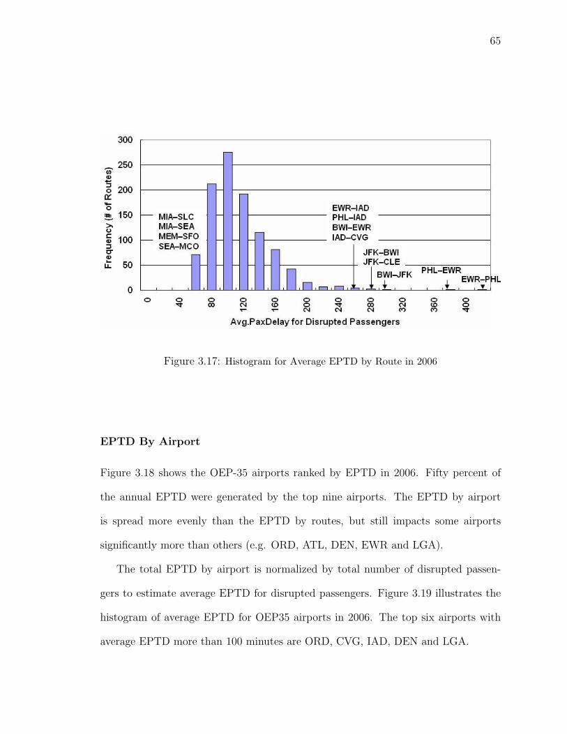
65
Figure 3.17: Histogram for Average EPTD by Route in 2006
EPTD By Airport
Figure 3.18 shows the OEP-35 airports ranked by EPTD in 2006. Fifty percent of
the annual EPTD were generated by the top nine airports. The EPTD by airport
is spread more evenly than the EPTD by routes, but still impacts some airports
significantly more than others (e.g. ORD, ATL, DEN, EWR and LGA).
The total EPTD by airport is normalized by total number of disrupted passen-
gers to estimate average EPTD for disrupted passengers. Figure 3.19 illustrates the
histogram of average EPTD for OEP35 airports in 2006. The top six airports with
average EPTD more than 100 minutes are ORD, CVG, IAD, DEN and LGA.

66
Figure 3.18: EPTD by Airport (Destination): Fifty Percent of the Annual EPTD is Gen-
erated by the Top 9 OEP-35 Airports
Rank of airports by average EPTD results in a different sequence than the rank
of airports by total EPTD. In particular, Atlanta Hartsfield-Jackson (ATL) Interna-
tional Airport, despite being ranked second by total EPTD, is ranked 19th by aver-
age EPTD. That means the large amount of total EPTD at ATL is mainly caused
by high passenger throughput instead of heavily delayed passengers. On the con-
trary, Washington-Dullas airport is ranked 19th by total EPTD, but ranked third
by average EPTD. This indicates disrupted passengers at Washington-Dullas airport
experienced a very high average delay, though the airport is relatively small with
fewer total enplanements.

67
Figure 3.19: Histogram for Average EPTD by Airport in 2006
3.3.4 Heavily Skewed Distribution of EPTD
A statistical comparison of the distributions of on-time percentage and delay magni-
tude for flights and passenger trips is performed in this subsection (Wang et al., 2007
B). The underlying behavior of flight delays and passenger trip delays are represented
by the right-tailed distribution in Figure 3.20. There are three pairs of parameters
used to characterize the delays:
1. Percentage of flights (or passengers) that arrive within 15 minutes of scheduled arrival
time (-∞, 15] (see (1) in Figure 3.20).
2. Average delay for flights (or passengers) that arrive within 15 minutes of scheduled
arrival time. Here the author assumes all on-time flights (or passengers) have a zero-
minute delay (see (2) in Figure 3.20).

68
Figure 3.20: Right-tailed distribution of flight (or passenger) delays. Identifies 3 pairs of
parameters used in this paper to characterize the distribution. Distribution for passenger
trip delay has similar form with longer right-tail.
3. Percentage of flights (or passengers) that arrive after 15 minutes of scheduled arrival
time, but less than the time associated with 95th percentile delays (see (3) in Figure
3.20).
4. Average delay for flights (or passengers) that arrive after 15 minutes of scheduled
arrival time, but less than the time associated with 95th percentile delays (see (4) in
Figure 3.20).
5. Five percent of flights (or passengers) that arrive after the 95th percentile delays (see
(5) in Figure 3.20).

69
6. Average delay for flights (or passengers) that arrive after the 95th percentile delays
(see (6) in Figure 3.20).
Passenger trip delays include the delays experienced by passengers due to delayed
flight, plus the delays accrued by waiting to be re-booked on a later flight when
a flight is cancelled. As a consequence, the distribution for passenger trip delays
exhibits a longer right tail. The question that is being resolved by this paper is: “Is
the magnitude of the right tail for passenger trip delay statistically significant when
compared to the right tail of flight delays?”
Calculating Flight Delay Parameters
• “15-OTP On-Time Flights Percentage”
For each route, the number of on-time flights (with less than 15 minutes) is summed.
This total is divided by the total number of scheduled flights on that route yielding
the 15-OTP On-Time Percentage of Flights for the route.
• “Average Magnitude of Flight Delays”
For each route, the flight delays for delayed flights (with flight delay more than 15
minutes) are summed. This total is divided by the total number of delayed flights on
that route yielding the Average Magnitude of Flight Delays for the route.
• “Average Worst-Case Magnitude of Flight Delays”
For each route, the top 5% flights with the largest flight delay are derived. Their
flight delays are summed. This total is divided by the total number of these top 5%
flights yielding the Average Magnitude of Flight Delays for the route.

70
Calculate Passenger Delay Parameters
• “15-POTP Passenger On-Time Percentage”
For each route, the number of passengers that are schedule on on-time flights (with
flight delay less than 15 minutes) is summed. This total is divided by the total number
of passengers on that route yielding the 15-POTP On-Time Percentage for Passenger
for the route.
• “Average Magnitude of Passenger Trip Delays”
For each route, the TPTP is first calculated, and then divided by the total number of
disrupted passengers (with PaxDelay more than 15 minutes) on that route yielding
the Average Magnitude of Passenger Trip Delays for the route.
• “Average Worst-Case Magnitude of Passenger Trip Delays”
For each route, the top 5 percent passengers with the largest passenger trip delay are
derived. Their passenger trip delays are summed. This total is divided by the total
number of the top 5 percent passengers yielding the Average Magnitude of Passenger
Trip Delays for the route.
Figure 3.21 provides a sample of Flight Delay statistics and Passenger Trip Delay
statistics generated by this analysis. By examination, 15-OTP and 15-POTP exhibit
similarity, but the distinction between the two sets of Flight Avg. Magnitude and
Passenger Average Magnitude are clearly evident.

71
Figure 3.21: Sample Statistics for Flight Delays and Passenger Trip Delays Statistics
First Pair of Parameters: 15-OTP v.s. 15-POTP
Figure 3.22 shows the histograms of Flight On-time Percentage and Passenger On-
Time Percentage. The 15-OTP and 15-POTP distributions exhibit similarities. Among
the 1030 routes, routes with the worst on-time percentages are EWR-PHL(47%),
JFK-CLT(48%), JFK-ORD(50%), PHL-EWR(53%) and JFK-DFW(55%). Overall,
the NAS has 77% of on-time flights with standard deviation equals to 7%.

72
Figure 3.22: Histograms of Flight Percentage of On-Time and Passenger Percentage of
On-Time (15-OTP v.s. 15-POTP)
Second Pair of Parameters: Average Magnitude of Flight Delay v.s. Av-
erage Magnitude of PaxDelay
Figure 3.23 shows the histograms of Average Magnitude of Flight Delays and the
Average Magnitude of Passenger Trip Delays. In 2005, the average delay across all
flights was 8 minutes. The average delay for those flights with delays in excess of 15
minutes on the OEP-35 routes ranged from 29 minutes (Salt Lake City - Washington
National) to 122 minutes (Honolulu - Minneapolis) with an average of 55 minutes.
The worst 5% delays ranged from 28 minutes (Portland - Chicago Midway) to 301
minutes (Honolulu - Minneapolis) with an average delay of 118 minutes.
The Average Magnitude for passenger trip delays exhibits a heavier right tail and
larger mean than the Average Magnitude for flight delays (δσ = 34 min and δµ = 21

73
min). This divergence is caused by cancelled flights. The top 7 routes with largest
Average Magnitude of Passenger Trip Delay are BWI-PIT (203min), CVG-MDW
(258min), EWR-PHL (238min), JFK-PHL (253min), MDW-CVG (256min), PHL-
EWR (298min), and PHL-JFK (209min). Many of these routes are short-haul routes
serving shuttle flights with high frequency, small aircraft size, and high cancellation
rate. The high cancellation rate results in large passenger trip delays.
Figure 3.23: Histograms of Average Magnitude of Flight Delays and Average Magnitude
of Passenger Trip Delays
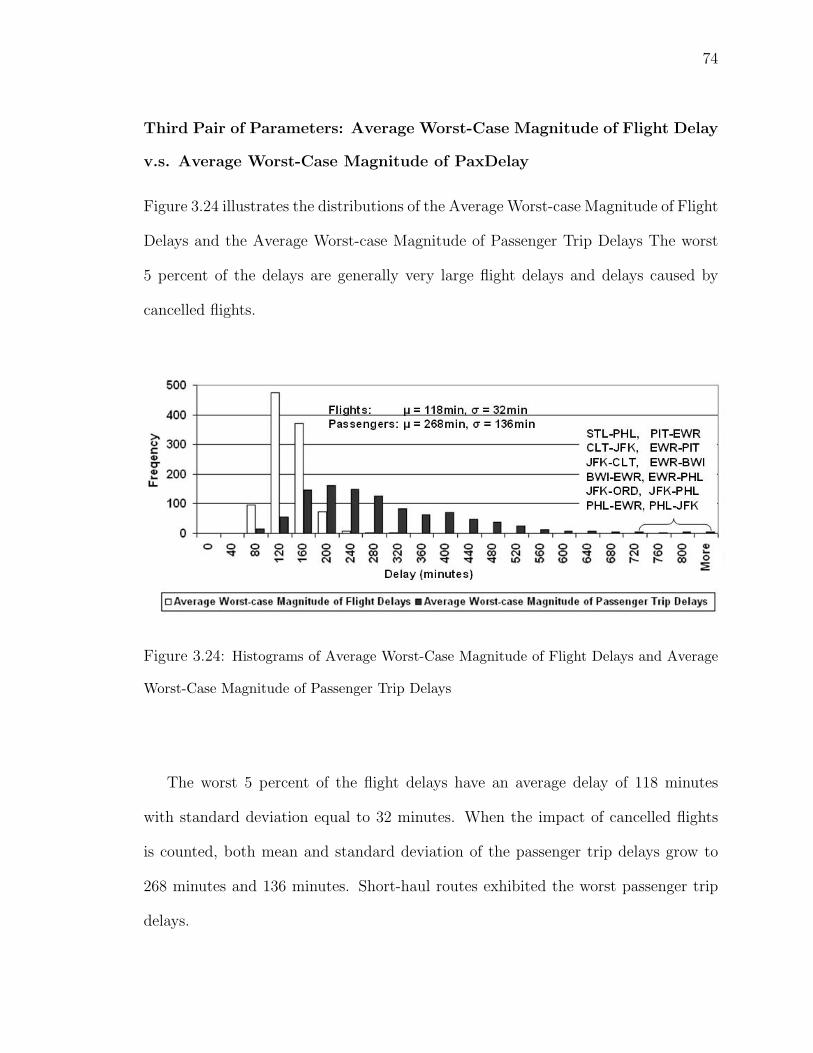
74
Third Pair of Parameters: Average Worst-Case Magnitude of Flight Delay
v.s. Average Worst-Case Magnitude of PaxDelay
Figure 3.24 illustrates the distributions of the Average Worst-case Magnitude of Flight
Delays and the Average Worst-case Magnitude of Passenger Trip Delays The worst
5 percent of the delays are generally very large flight delays and delays caused by
cancelled flights.
Figure 3.24: Histograms of Average Worst-Case Magnitude of Flight Delays and Average
Worst-Case Magnitude of Passenger Trip Delays
The worst 5 percent of the flight delays have an average delay of 118 minutes
with standard deviation equal to 32 minutes. When the impact of cancelled flights
is counted, both mean and standard deviation of the passenger trip delays grow to
268 minutes and 136 minutes. Short-haul routes exhibited the worst passenger trip
delays.

75
Statistical Comparison Between the Three Pairs of Parameters
Table 3.4 summarizes the statistics over all 1030 routes formed by OEP-35 airports.
By inspection of the table, percentage of on-time flights is similar to the percentage
on-time passengers. The mean of the average delay for flights delayed in excess of 15
minutes is 34 minutes lower than the mean of the average delay for passenger trips.
The average worst-case flights delays in excess of the 95th percentile is 150 minutes
lower than average worst-case passenger delays in excess of the 95th percentile.
Table 3.4: Comparison of Statistics for Distribution of Flight Delays and Distribution of
Passenger Trip Delays
Percentage On-
Time
Mean Average
Magnitude of
Delays
Mean Average
Worst-Case Mag-
nitude of Delays15-OTP 15-POTP Flights Passengers Flights Passengers
Average 0.7729 0.7726 53 87 118 268Standard Devia-
tion
0.072 0.073 9.1 30.2 32.0 136.4
The worst 5% (ex-
cess 95 percentile)
0.977 0.877 68 138 170 510
Paired t-tests and χ2 tests are performed on the above three sets of Flight Delay
and Passenger Trip Delay metrics. A paired t-test of percentage on-time across all
routes can not reject the null hypothesis that Passenger On-Time Percentage has the

76
same distribution mean as Flight On-Time Percentage (P-value 0.1858, 95% confi-
dence interval -0.000015, 0.0008). The test cannot reject the null hypothesis that the
Passenger On-Time Percentage and Flight On-Time Percentage have equal variance
(P-value 0.5618). The scattered plot shows a highly linear relationship (R2=0.99) be-
tween Passenger On-Time Percentage and Flight On-Time Percentage. Altogether,
there is no significant evidence to claim the hypothesis that the distribution of Flight
On-Time Percentage is different to the distribution as Passenger On-Time Percent-
age. A paired t-test cannot reject the null hypothesis that the distribution mean of
the “Average Magnitude of Passenger Trip Delays” is 34 minutes in excess of the
distribution mean of the “Average Magnitude of Flight Delays” (P-value 0.9985, 95%
confidence interval -1.633, 1.6304). A paired t-test can not reject the null hypothe-
sis that the distribution mean of “Average Worst-Case Magnitude of Passenger Trip
Delays” is 150 minutes in excess of the distribution mean of “Average Worst-Case
Magnitude of Flight Delays” (P-value 0.9704, 95% confidence interval -7.545, 7.2642).
χ2 tests do reject the hypothesis that both of the above two distributions (Average
Magnitude of Delays, and Average Worst-Case Magnitude of Delays) have equal vari-
ance. Both p-values are less than 0.001. The distributions of 15-POTP “Magnitude of
Delay” metrics are significantly wider than the distributions of 15-OTP “Magnitude
of Delay” metrics The results of the t-tests and χ2 tests quantify the non-negligible
difference in the magnitude of delays experienced by passengers.
Overall, the statistical results above conclude that the Flight Delays do not repre-
sent a fair description of the performance of Passenger Trip Delays between OEP-35
airports. The passenger trip delays in excess of the flight delays are not negligible.
With an average of 34 minutes difference between average delays across all routes and

77
2.5 hours difference between the average worst-case delays, the passenger trip delays
affect passenger connections to other flights as well as other modes of transportation.
These results have significant implications for the way passengers think about air
transportation and flight choice, and the way consumer protection of airline travelers
is provided.
Integrating Probability of Delay with Magnitude of Delay
Passenger choices of flights from and to large metropolitan areas have expanded over
the past decade to include choice of departure and arrival airport. For example,
Boston, New York, Washington D.C., San Francisco, Los Angeles, and South Florida
are all serviced by multiple airports. The choice of airport pairs provides the passenger
with an additional degree of freedom in selecting flights. 15-POTP for routes between
the Washington, D.C. and Chicago are shown in Table 3.5. The most reliable routes
are ranked by Passenger On-Time Percentage (i.e. 15-POTP). But the routes with
the least passenger trip delay are ranked by average magnitude of passenger trip delay.
Figure 3.25 plots the statistics in Table 3.5 in two charts. The chart area is di-
vided into four blocks. Routes in the upper-left block are the most reliable routes that
have high passenger on-time percentage and low average magnitude of passenger trip
delays. The highest reliability route is DCA to MDW with a 14 percent differential
over routes departing IAD for either ORD or MDW, and 10 percent differential for
flights on the BWI to MDW route. Risk-averse passengers with scheduled connecting
time less than 1.5 hours might prefer the second reliable route BWI-MDW, since it
has the lowest Magnitude of Passenger Trip Delays.

78
Table 3.5: Example of Using 15-POTP for Purchasing Airline Tickets
Most Reliable RoutesRanks Origin Dest 15-
POTP
Avg. Magnitude of
PaxDelay
Average Worst-Case
Magnitude of PaxDelay1 DCA MDW 92% 120 171
2 BWI MDW 82% 67 1472 BWI ORD 82% 102 2954 DCA ORD 80% 123 3645 IAD ORD 78% 103 3426 IAD MDW 76% 152 565
Routes with Least Passenger Trip DelayRanks Origin Dest 15-
POTP
Avg. Magnitude
of PaxDelay
Average Worst-Case
Magnitude of PaxDelay1 BWI MDW 82% 67 147
2 BWI ORD 82% 102 2953 IAD ORD 78% 103 3424 DCA MDW 92% 120 1715 DCA ORD 80% 123 3646 IAD MDW 76% 152 565
Figure 3.25: Plots of Reliability of Routes Between Washington D.C. and Chicago

79
3.3.5 ATNAT Tool
Transportation systems are commonly represented using networks as an analogy for
their structure and flows. The Air Transportation Network physically consists of
airports(nodes) and routes(arcs). These airports and routes are NOT homogeneous.
They have specific behavior patterns that form the network properties. Moreover,
EPTD has asymmetric performance for different airports and routes. Some simple
strategies can be used by passengers to avoid high risk of delay, such as choosing
a different departure time, airport or airline. An example is given in the previous
section (Table 3.5 and Figure 3.25).
The Air Transportation Network Analysis Tool (ATNAT) is deigned to provide a
single source of statistical information about the performance of the routes, airports
and airlines in the Air Transportation Network in 2004. It supports informed decisions
of passengers by helping them better understand the historical performance of the
route/airline combination.
Airports and Airlines Included
See Table 3.6.
Combinations of Information
By default, information is displayed as a daily average per O+D/airline combination
(Figure 3.26). The number of days in the data set is displayed at the top-left corner
of the table. This top-left designator will be referred to as the “subset identifier.”

80
Table 3.6: Airports and Airlines Included in the ATNAT Tool
Airport AirlineATL LAX American (AA)BOS LGA Alaska (AS)BWI MCO JetBlue (B6)CLE MDW Continental (CO)CLT MEM Independence (DH)CVG MIA Delta (DL)DCA MSP Atlantic Southeast (EV)DEN ORD Airtran (FL)DFW PDX Hawaiian (HA)DTW PHL America West (HP)EWR PHX American Eagle (MQ)FLL PIT Northwest (NW)HNL SAN Comair (OH)IAD SEA Skywest (OO)IAH SFO Express Jet (RU)JFK SLC ATA (TZ)LAS TPA United (UA)LAX US Airways (US)LGA Southwest (WN)
Rank is based on the magnitude of the value (not the benefit/cost) for all O+D’s. In
other words, the largest figure of on-time performance will be ranked first as well as
the largest number of disrupted passengers per day. The subset identifier and rank
profile changes based on the selections by the user. Figure 3.27 indicates the different
selections and their respective impact.

81
Figure 3.26: The Air Transportation Network Analysis Tool (ATNAT)
Figure 3.27: Combinations of Inputs and Outputs for ATNAT

82
Example
Route DFW-ATL and Route MSP-ORD share many operational similarities. As
shown in Figure 3.28, they both have four airlines operation on the routes. They
operated on average 30 flights per day (2-1), eight of them were delayed (2-3). On
both routes, 72 percent of passengers arrived on-time(1-1). However, route DFW-
ATL had larger aircraft (3-1), higher load factors (3-2 and 3-3), and less cancellation
(2-2) than the MSP-ORD route. These three factors are critical to determine the
delays on passenger trip. Divergence between these two routes in the “passenger
experience” category is clearly evident. More passengers were transferred and more
passenger delays were generated on route DFW-ATL, because it has larger aircraft
and higher load factors. But when passenger delay is normalized by enplanement,
route MSP-ORD has higher “expected individual passenger delay” (26 minutes per
enplanement) than route DFW-ATL (18 minutes per enplanement). Fourteen percent
of passengers on route MSP-ORD experienced delays of more than one hour, while
only 9 percent experienced delays on route DFW-ATL.

83
Fig
ure
3.28
:St
atis
tic
Par
tsof
GU
Ifo
rR
oute
sD
FW
-AT
Lan
dM
SP-O
RD

84
Figure 3.29: Graphic Parts of GUI for Routes DFW-ATL and MSP-ORD
Figure 3.29 shows the graphic illustration part of the ATNAT tool for both routes.
The upper two graphs notify users of the likelihood that they would be delayed on
each route. For example, on route DFW-ATL, 9.7 percent of passengers were delayed
by 15-30 minutes, 8.8 percent of them were delayed by 30-60 minutes, and 5.8 percent
of them were delayed by one to two hours. The yellow bar represents the passenger
delay proportion caused by cancelled flights. Passengers on route DFW-ATL are more
likely to encounter short delays while passengers on route MSP-ORD have higher risk
of long delays. The two lower graphs illustrate the passenger risk of encountering long
delays (more than one hour) in terms of scheduled departure time. According to the
graphs, passengers on both routes should avoid booking flights scheduled to depart
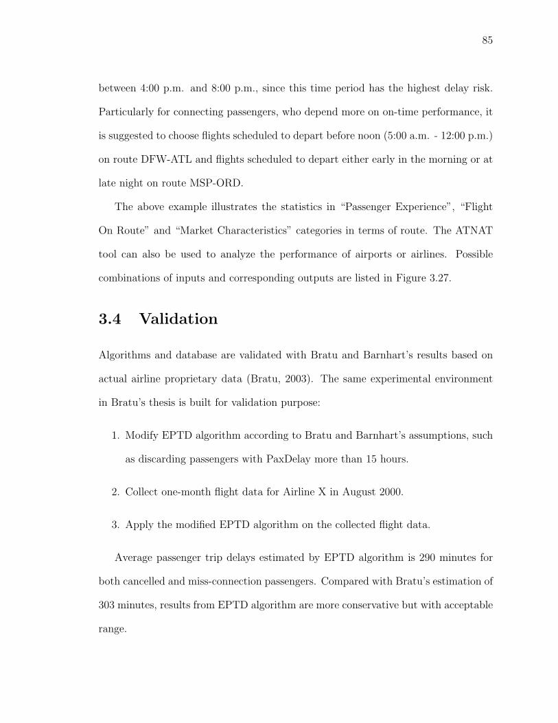
85
between 4:00 p.m. and 8:00 p.m., since this time period has the highest delay risk.
Particularly for connecting passengers, who depend more on on-time performance, it
is suggested to choose flights scheduled to depart before noon (5:00 a.m. - 12:00 p.m.)
on route DFW-ATL and flights scheduled to depart either early in the morning or at
late night on route MSP-ORD.
The above example illustrates the statistics in “Passenger Experience”, “Flight
On Route” and “Market Characteristics” categories in terms of route. The ATNAT
tool can also be used to analyze the performance of airports or airlines. Possible
combinations of inputs and corresponding outputs are listed in Figure 3.27.
3.4 Validation
Algorithms and database are validated with Bratu and Barnhart’s results based on
actual airline proprietary data (Bratu, 2003). The same experimental environment
in Bratu’s thesis is built for validation purpose:
1. Modify EPTD algorithm according to Bratu and Barnhart’s assumptions, such
as discarding passengers with PaxDelay more than 15 hours.
2. Collect one-month flight data for Airline X in August 2000.
3. Apply the modified EPTD algorithm on the collected flight data.
Average passenger trip delays estimated by EPTD algorithm is 290 minutes for
both cancelled and miss-connection passengers. Compared with Bratu’s estimation of
303 minutes, results from EPTD algorithm are more conservative but with acceptable
range.

Chapter 4: Passenger Flow Simulation (Methods
and Results)
In the previous chapter, algorithms and databases were developed to achieve the “his-
torical analysis” of the passenger trip experience, and to understand the correlations
between the delay performance of the vehicle tier and the passenger tier of the ATS.
The historical analysis cannot be used to predict the impact of future policy changes
on passenger trip time. Also, the algorithms do not include the passenger trip delay
caused by missed connections.
In this section, a stochastic passenger-based simulation model is built to capture
the impact of missed connections on passenger trips and evaluate the system perfor-
mance outside the range of historical data. The “historical analysis” provides unique
route and airport properties (e.g. distributions of taxi-in time, taxi-out time and air
time) for the passenger flow simulation (PFS). PFS simulates passenger flow through
the network and predicts impacts on passenger performance given changes in sys-
tem design, rules and performance. Experiments are performed to identify significant
factors affecting passenger performance.
86

87
4.1 The Underlying Concept
Air transportation simulations of flight movement do not capture the passenger flow
and connecting process. In the Air Transportation Network, passengers cluster to-
gether into groups to fly from one airport to another. After arriving at the destination
airport, this group of passengers break up: nonstop passengers make connections to
ground transportation, and connecting passengers continue their trips by re-clustering
with other passengers. As illustrated in Figure 4.1, the re-clustered passenger group
consists of both local passenger who just entered the system, and connecting passen-
gers who came from other origin airports.
Figure 4.1: Underlying Concepts for Passenger Flow Simulation Model
The passenger flow simulation (PFS) model is built to simulate the dynamical
clustering and scattering process of passenger flow in the ATS. Compared with the

88
flight-based simulation model, PFS:
• Converts flight unit to a passenger unit,
• Converts flight information, such as arrival time, departure time, Origin-Destination
pair, etc., into attributes of passenger,
• Converts flight schedule into clustering and scattering rules followed by passen-
gers.
In summary, this idea converts the “flight” concept into the “passenger” concept.
4.2 Petri Net Modeling Tool
A Petri Net is a graphical and mathematical modeling tool. It is well-suited to model
a public transportation network because it is designed to model the asynchronous
behavior of the different transport modes and the synchronization between buses,
trains, subways and passengers when a set of passengers gets on or gets off a mode
of transport (Castelain and Mesghouni, 2002). Petri Nets have been used to model
the passenger connecting process in the public bus transportation system (Turki et
al., 2002), (Turki et al., 2003), (Castelain and Mesghouni, 2002).
For an accurate modeling of a complex transportation system like the air trans-
portation system, a more complicated extension of Petri Net is required. In this
dissertation, a hierarchical, timed, colored petri net (CPN) is built in “CPN Tools”
to simulate passenger flow and connecting process in the air transportation network.
“CPN Tools” is a Graphic User Interface (GUI) tool for editing, simulating and ana-
lyzing Colored Petri Nets. Detailed information information of CPN Tools is available
on http://wiki.daimi.au.dk/cpntools/cpntools.wiki

89
CPN Tools can model the complex level of interactions in the ATS visually by
creating nodes, transitions and arcs in the model environment. This visual modeling
environment allows people to track and understand the behavior of each passenger
easily. In addition, the object-oriented properties and the hierarchical structure that
can be achieved in CPN Tools simplify the model structure. They allow the user to
clone nets without re-building the whole net.
For the purpose of this research, there are three more reasons to choose colored
petri nets:
1. It can present the idea of passenger clustering and scattering through the net-
work by using “colored tokens” to represent different groups of passengers.
2. It can differentiate routes and passengers, and identify the distinct properties
of each arc and node that compose the network by defining CPN attributes,
guard function, arc expression, etc.
3. It can update policies, options and strategies fairly easily by changing arc func-
tions and guard functions in the model.
More detailed introductions on Petri Nets, Colored Petri Nets, Hierarchical Petri
Nets, and Timed Petris Nets are available in Chapter 2.3.1.
4.3 Structure of Passenger Flow Simulation (PFS)
The Operational Evolution Plan (OEP) 35 airports are the nation’s busiest airports
defined by the FAA (FAA, 2004). They have the greatest number of operations
and account for 73 percent of total enplanements and 69 percent of total operations

90
in the air transportation system (Bhadra and Texter, 2005). The Passenger Flow
Simulation (PFS) is a closed network formed by 34 of the OEP-35 airports. Honolulu
International Airport (HNL) is excluded due to its geographic location and negligible
impact on the network.
4.3.1 PFS Overview
Table 4.1 lists overview statistics for the Passenger Flow Simulation (PFS) model:
Table 4.1: Overview of Passenger Flow Simulation Model
Airports OEP-34 Airports (excluding HNL)Routes 1,030 routes formed by OEP34 air-
portsMajor Carriers 17 major carriersDaily Flights 8,500Daily Enplanements 900,000PFS Mode Deterministic PFS and Stochastic
PFSHierarchy 3-LevelPlaces 580Transitions 343Initial Tokens 20,000Functions 42
4.3.2 PFS Color Definition
The concept of “color” distinguishes tokens (or resources) in the net. “PaxGroup” is
defined as a color in PFS:

91
Color: PaxGroup = (Origin) * (Dest) * (# of Pax Loaded) * (AircraftSize) * (SchDep-
Time) * (SchArrTime) * (Carrier) * (FlightIndex) * (# of Local Pax) timed;
Figure 4.2 illustrates an example of the passenger boarding process. The Pax-
Group (DCA, ORD, 185, 200, 730, 850, 13, 45, 165)@+ 750 means 185 passengers
are loaded on an aircraft with 200 seats to fly from Washington-National (DCA)
Airport to Chicago O’Hare (ORD) Airport. This flight was scheduled to depart on
system time 730, and arrive on system time 850. But it actually departed on system
time 750, 20 minutes later than scheduled. The flight is operated by United Airlines,
with flight index 45. Within the 180 loaded passengers, 165 are local passengers
whose itinerary destination is ORD.
Figure 4.2: Example: Passenger Boarding Process
Two groups of connecting passengers are supposed to be loaded on flight 45. The
first group with 20 connecting passengers successfully boarded, because they arrived

92
at the boarding gate before the actual departure time of flight 45. But the second
group of 15 passengers arrive at the boarding gate at system time 770, which is 20
minutes later than the departure of flight at system time 750. This group of 15
passengers are “missed-connection passengers” in the system.
4.3.3 PFS Declaration
The PFS declaration includes definitions of functions, color, variables, values and
output files. All of these are listed in Appendix D.
4.3.4 PFS Hierarchy
The passenger flow simulation model has three levels as illustrated in Figure 4.3.
Airport and en route subnets are represented as substitute transitions in the top-level
page of PFS. Detailed explanation and zoom-in figures of top-level, second-level and
the third-level nets are available in the subsequent subsections.

93
Figure 4.3: Three-Level Hierarchy of Passenger Flow Simulation Model
4.3.5 PFS Top Level Net
The top-level page of PFS is illustrated in Figure 4.4. It depicts 34-airport substitute
transitions, a single en route substitute transition, and the 68 ports connecting them.
A zoom-in figure of Washington-National (DCA) airport shows an aggregated depar-
ture gate and an aggregated arrival gate for each airport. An airport substitution
transition is directionally connected to/from route substitution transition through
two ports: one represents arrival gate and the other represents departure gate.

94
The “air-side” gate-to-gate transportation of passengers is accomplished by flowing
sequence departure gate→ en route→ arrival gate. Joining the process of connecting
passengers happens within the airport substitution transition which belongs to level
two and cannot be observed from the top-level page.
Figure 4.4: Top Level Page for 34-Airport PFS

95
4.3.6 PFS En route Subnet (2nd Level)
Figure 4.5 gives an example of a single route substitution transition (ATL-LGA). En
route is an air-side gate-to-gate process. Four time points, out-of-the-gate, off-the-
ground, on-the-ground and into-the-gate, referred to in the industry as “OOOI”, can
be used to describe the en route process.
Figure 4.5: Enroute Subnet for a Single Route (ATL-LGA) for 4-Airport PFS
The time difference spent on the taxiway between “out-of-the-gate” time point to
“off-the-ground” time point is defined as taxi-out-time (or transition time for “Taxo-
Out Process”). Similarly, the time difference spend on the taxiway between “on-
the-ground” time point to “into-the-gate” time point is defined as taxi-in-time (or
transition time for “Taxi-In Process”). “Air-time” is the time period after the depar-
ture from runway and before the arrival at runway, that is, the time difference between
“off-the-ground” and “on-the-ground.” Passengers take off from the departure gate
at time “out-of-the-gate,” and are ready to depart on the runway after taxi-out-time.
After flying for some time period (air time), passengers arrive at the runway at time

96
point “on-the-ground,” and arrive at the gate after the taxi-in process. Transitions
with “C” on the lower-right corner are transitions with code segments. All the codes
written in Standard Meta Language (SML) are provided in Appendix E.
Figure 4.6 depicts the aggregated en route subnet for 1,030 routes formed by the
34 OEP airports in 2006. Instead of having a pair of departure and arrival ports for
each route, the PFS has 34 departure ports and 34 arrival ports in total. PFS reads
itinerary information from the passenger groups appearing at departing ports, and
guides them to the right routes until arriving at the correct arrival ports.

97
Fig
ure
4.6:
Enr
oute
Subn
etfo
r34
-Air
port
PF
S

98
4.3.7 PFS Airport Subnet (2nd Level)
An airport substitution transition is much more complicated than a route substitution
transaction. It contains passenger connecting, scattering and re-clustering processes
within the boundary of one airport.
Figure 4.7 shows the airport subnet for ORD as an example. In this figure, all
the arc expressions and code segments are in hidden status for a clear and clean
presentation of the airport subnet structure. Passenger groups (PaxGroup) flow into
the airport boundary from arrival gates on the top of Figure 4.7, and flow out of the
airport boundary from departing gates on the left side of Figure 4.7. This flowing
process is divided into three steps: (1) splitting PaxGroup, (2) re-clustering of Pax-
Group and (2) loading PaxGroup. Figure 4.8, Figure 4.9 and Figure 4.10 illustrate
the three steps of passenger flow respectively.

99
Figure 4.7: Airport Subnet (ORD) for 4-Airport PFS
Step 1: Splitting PaxGroup
As shown in Figure 4.8, PaxGroup flows into the airport boundary from arrival gates.
In this specific example, arrival gates are: place “Arrivals ATL-ORD,” place “Arrivals
LGA-ORD” and “Arrivals MEM-ORD.” After arriving at ATL airport, the PaxGroup

100
splits into two subgroups: “Local Arrivals” and “Connecting Arrivals”. Passengers
belonging to “Local Arrivals” end their itineraries at ATL, while passengers belonging
to “Connecting Arrivals” continue their itineraries for the second-leg flights from ATL.
“Local Passengers” are passengers whose itineraries end right after the flight ar-
rives at the destination airport. They include not only non-stop passengers, but also
connecting passengers whose itinerary destination is the destination airport of the
segment flight. “Connecting passengers” are passengers who only stay at the airport
for flight connection.
Figure 4.8: Step 1: Splitting PaxGroup at ORD airport
The ratio of connecting and local passengers in terms of route are obtained from
the DB1B* database. For this specific example shown in Figure 4.8, passengers
coming from ATL to ORD consist of 78 percent of the local passengers and 22 percent
connecting passengers. This means 78 percent of passengers coming from ATL end
their itineraries at ORD. The “airport groups” in DB1B table (see Figure ??) for this

101
78 percent passengers are either “ATL-ORD,” or “X-ATL-ORD.” Airport X could
be any airports except for ATL or ORD. The other 22 percent of passengers are
connecting passengers who come from ATL and connect at ORD (ATL-ORD-X).
Step 2: Re-clustering PaxGroup
A minimum amount of time, called Minimum Connecting Time (MCT), is required
to guarantee a smooth connection of passengers and baggage delivery. Example in
Figure 4.9 depicts the process of connecting and re-clustering at ORD.
Figure 4.9: Step 2: Re-clustering PaxGroup at ORD airport
The minimal connecting time is directly collected from airlines by the Official
Airline Guide (OAG). This OAG-collected MCT is essential when constructing air
transport schedules, because it is the time required for transferring not only passengers

102
and also baggage between flights. In general, airlines will schedule sufficient time for
passenger and baggage connection. However, the actual time for passengers to walk
from one gate to another could be much less than the given connecting time. Here
the author assumes the MCT for passengers to walk from one gate to another is
half of the MCT collected by the OAG. For example, MCT collected by the OAG
for Chicago O’Hare airport (ORD) is 50 minutes, meaning the MCT for connecting
passengers at Chicago O’Hare would be 25 minutes.
There are two functions involved in the code segment. One is the function “fun-
MCT(airport),” which returns the minimal connecting time required for passengers
between gates given connecting airport. The other function is an arc function, which
divides a group of connecting passengers into several subgroups and sends them to
different gates. For example, Continental Airlines only has connecting flights to Cleve-
land Hopkins (CLE) Airport, Newark (EWR) Airport and Houston (IAH) Airport
connecting at Chicago O’Hare (ORD) Airport. If Continental Airlines has a connect-
ing PaxGroup of 100 people arriveing at ORD, 28 of the 100 passengers will go to
CLE, 32 passengers will go to EWR airport and 40 passengers will go to IAH. The
passenger flow ratio and airport connecting information is obtained from DB1B* data
(see Figure ??). Let P = total number of passengers in format “X-ORD-Y,” and P1
= total number of passenger in format ‘X-ORD-IAH” (airport X and Y could be any
airport except ORD). Then ratio P1/P is the proportion of connecting passengers
flowing from ORD to IAH.

103
Step 3: Loading PaxGroup
Passengers who showed up before the actual departure time will be successfully
loaded, while passengers who failed to show up on time have to wait to be re-booked
on the next available flight.
Figure 4.10: Step 3: Loading PaxDelay at ORD airport
As shown in Figure 4.10, places “toATL,” “toLGA” and “toMEM” represent
the boarding gates from ORD to ATL, LGA and MEM, respectively. Connection
passengers reside in these “gate” places. Substitute transitions such as “Clustering

104
Pax at ORD to ATL” are responsible to load connecting passengers on the right flights
with local passengers. Flights stop loading passengers when either the departure time
is on schedule, or no more seats are available. When the system time reaches the
actual departure time of flight, it pushes back from the gate to the taxiway.
The subnet for substitute transition “Cluster Pax at ORD to ATL” will be ex-
plained in the next part: Passenger Loading Subnet(3rd Level)
4.3.8 PFS Passenger Loading Subnet(3rd Level)
Passengers coming from socket “toATL” are divided into two groups: (1) general
connecting passengers flow to the upper branch, and (2) miss-connection passengers
and cancelled passengers flow to the lower branch. The general connecting passengers
(upper branch) have higher priority than cancelled or missed-connection passengers
(lower branch). Passengers on both branches are sorted into first-come-first-serve air-
line queues to ensure only passengers belonging to this airline can be loaded on flights
operated by this airline. Flights with loaded local passengers reside in place “Local
Pax ORD-ATL.” When transition “Load Connecting Pax ORD-ATL” fires, it loads
general connecting passengers, and generates a token in place “Ready PaxGroup”
representing “ready to depart.” But before it actually departs, the flight checks the
airline queue on the lower branch for missed connection or cancelled passengers. If
there are missed connection or cancelled passengers waiting to be re-booked, and the
flight still has empty seats, it begins loading the re-booked passengers until either no
more empty seats are available, or no more re-booked passengers that are available
to be re-booked before the departure time of the flights. Note, the underlying rule
is, cancelled or missed connection passengers can only be re-booked to flights on the

105
same route and operated by the same airline as scheduled.
Figure 4.11 shows the third-level subnet of the PFS. It depicts the loading process
at the departure gate.

106
Fig
ure
4.11
:P
asse
nger
Loa
ding
Subn
etfo
rR
oute
OR
D-A
TL

107
There are three transitions with code segment in Figure 4.11:
• The code segment in the “Adjust” transition ensures that connecting passengers
will go to the booked flights instead of jump on any available flight. This is
the difference between air transportation and bus transportation. Passengers
buy air tickets before the trip, and they have to follow the itinerary unless
it is disrupted by overbooking, a cancelled flight, and missing a connection.
Passengers in the bus transportation system do not buy tickets until they get
on the bus. In other words, they have full control of the itinerary. Connecting
passengers in the bus transportation system can get on the next bus going to the
same destination. But connecting passengers in the air transportation system
have to wait for the connecting flights they booked, even if they arrive at the
gate early enough to catch an earlier flight to the same destination.
• the code segment in “Load Conn Pax ORD-ATL” exports connecting informa-
tion to a txt file named “Connection Results.” This is part of the PFS outputs.
• the code segment in “Load CancPax & MissConnPax ORD-ATL” exports re-
booking information to a txt file named “Rebooking Results.” This is part of
the PFS outputs.
4.3.9 Passenger Missed Connection Algorithm in PFS
Each specially designed experiment has two PFS models: one is called “Base-Scenario,”
and another is called “Experimental-Scenario.” “Base-Scenario” simulates passenger
flow in an ideal ATS without any disruptions, such as flight delays or flight cancella-
tions. All flights or PaxGroups depart and arrive at the scheduled time. The major

108
function of this “Base-Scenario” is to estimate passenger connecting information. In
other words, the “Base-Scenario” simulates passenger booking process: when passen-
gers purchase air tickets online, they choose connecting flights based on the scheduled
flight information: that is, passengers assume an ideal ATS without delay and can-
cellation.
Figure 4.12 gives an example of purchasing an air ticket online. The itinerary IAD-
LAS-SFO in the example is from Washington-Dullas (IAD) airport to San Francisco
(SFO) airport, connecting in Las Vegas (LAS) airport.
Figure 4.12: Example of Purchasing Air Ticket Online
The first-leg flight from IAD to LAS is scheduled to arrive at 7:13 pm. But there
are two options for the second-leg flight. The only difference between option 1 and 2 is
the scheduled connecting time. Option 1 has 50 minutes connecting time and option
2 has one hour and 29 minutes connecting time. This author assumes passengers
will most likely choose the first option because it is more time-effective than waiting

109
an additional 39 minutes. Based on this assumption, the ideal scenario is executed,
producing the estimated passenger connecting information for all connections in the
34-Airport PFS.
Figure 4.13 illustrates the process of estimating passenger trip delay in PFS.
“Base-Scenario” is the ideal scenario of ATS with no disruptions. The passen-
ger connecting information provided by Base-Scenario enables us to conduct re-
search on miss-connection in the “Experimental-Scenario.” The simulation results
of Experimental-Scenario estimate EPTD due to delayed flights, cancelled flights,
and miss-connections.
Figure 4.13: Estimate Passenger Trip Delay in PFS

110
4.4 Deterministic Passenger Flow Simulation (PFS)
PFS for the closed network formed by OEP 34 airports has two modes: deterministic
and stochastic. They share the same PFS structure, but with different functions and
parameter values. The deterministic PFS purely converts the flight performance to
passenger performance. The BTS database provides flight on-time performance data,
which contains the historical flight performance information such as departure delay
and arrival delay. In the deterministic PFS, each flight token departs and arrives at
the actual departure and arrival time with actual departure and arrival delay. In the
stochastic model, variables such as taxi-in, taxi-out and air-time, are given by normal
random number generators with specific means and standard deviations for flights
deparing from/arriving at different airport, or on the different routes. Thus the flight
arrival time (or arrival delay) is no longer deterministic.
Analysis on simulation results of deterministic PFS is described in the following
sections.
4.4.1 Simulation Results and Validation: 34-Airport PFS on
July 6 2005
July 6, 2005 is a randomly chosen weekday in summer 2005. This author chose
summer 2005 over summer 2006 because traffic in summer 2005 was heavier than the
traffic in summer 2006. Flight performance on July 6, 2005 is as follows:
• Scheduled Flights = 8,540 flights
• Delayed Flights = 1,764 flights = 21% of Scheduled Flights
• Cancelled Flights = 176 flights = 2% of Scheduled Flights

111
The “Experimental-Scenario” converts flight performance on July 6, 2005 into the
corresponding passenger performance.
Figure 4.14: Deterministic PFS Simulation Results for July 6 2005
As shown in Figure 4.14, 2 percent of cancelled passengers generated 30 percent
of total EPTD, 1 percent of missed connection passengers generated 15 percent of
total EPTD, and 21 percent of delayed passengers generated 55 percent total EPTD.
The 34-airport ATS generated 330,834 hours PaxDelay on July 6, 2005. On average,
passengers scheduled on cancelled flights experienced 403 minutes of delay, missed
connection passengers experienced 341 minutes of delay, and passengers scheduled

112
on delayed flights experienced 64 minutes of delay. The simulation results of 34-PFS
validate the asymmetric behavior of EPTD once more. Cancelled and miss-connection
passengers together only account for 3 percent of total enplanements, but generated
45 percent total EPTD with a high average delay of 382 minutes.
For validation purpose, the total EPTD and average EPTD estimated by EPTD
algorithm for July 6, 2005 are compared with these estimated by deterministic PFS.
Table 4.2 lists and compares the estimated total and average EPTD by EPTD algo-
rithm and deterministic PFS.
Table 4.2: Validation of Deterministic PFS
Deterministic PFS EPTD Algorithm Diff=|EPTD-PFS|/EPTD*100Total 309,000 hrs 306,000 hrs 1%Average 88 minutes 90 minutes 2%
“Diff” in Table 4.2 is calculated as: absolute value of (Algorithm - PFS) / Algo-
rithm * 100. The percentages of difference for total and average EPTD between these
two estimations are 1 percent and 2 percent respectively.
EPTD algorithm only estimates passenger trip delay due to delayed and cancelled
flights. Consequently, the total and average statistics listed in Table 4.2 do not include
EPTD due to missed connections. However, the estimated average EPTD due to
missed connections can be compared to Bratu and Barnhart’s result of 303 minutes
avearage delay for disrupted passengers. A subject of future work is to validate the
EPTD due to missed connections with more airline proprietary itinerary data.

113
In PFS, total EPTD generated by a delayed flight is adjusted by subtracting
the PaxDelay associated with missed-connection passengers who are supposed to be
loaded in this flight by not. The 183,000 hours of total EPTD due to delayed flights
shown in Figure 4.14 is adjusted by subtracting 28,000 hours of EPTD associated
with missed-connection passengers. In Table 4.2, the 28,000 hours of EPTD is added
back, because the validation excludes missed-connection passengers. This explains
why the total EPTD of 309,000 hours in Table 4.2 is 28,000 hours more than the
summation of EPTD due to delayed and cancelled flights in Figure 4.14.
4.4.2 Design of Experiment (DOE)
PFS analyzes the major trends in passenger flow dynamics to identify the critical
factors that affect passenger trip time most (such as load factor, distribution of flights,
etc.). In addition, specific scenarios can be generated to predict impacts on passenger
trip time given anticipated changes in the future.
Purpose of DOE
Experiments are designed for deterministic PFS to:
• Identify and rank order the significant factors that have strong impacts on
Passenger Trip Time
• Analyze the sensitivity of PaxDelay given changes in factors
Choice of Initial Significant Factors
Based on the literature (Bratu and Barnhart, 2005), six factors belonging to four
categories are chosen as initial significant factors (in Table 4.3):

114
Table 4.3: Initial Significant Factors and Their Categories
Categories FactorPassenger Factors (1) # of passengers loaded on a flightSeat Factors (2) Aircraft Size (# of total seats)
Flight Performance(3) Flight Cancellation Time(4) Flight Delay
Policy(5) Airline Cooperation Policy(6) Minimal Connecting Time (MCT)
Load factor equals “# of passengers loaded” divided by “aircraft size”. Flight can-
cellation time indicates the scheduled departure time of cancelled flights. This factor
is used to measure the difference between early cancellations and late cancellations.
Airline cooperation policy indicates airlines operating on the same route agree to help
each other re-book cancelled and missed-connection passengers. In other words, can-
celled or missed-connection passengers no longer need to stick with the same airline
during the re-book process. Minimal connecting time indicates the average time for
connecting passengers walking from one gate to another. This factor represents better
terminal structure and more efficient allocation of gates related to EPTD.
DOE Method
A full factorial design for six factors assuming a linear response function, needs 26=64
total runs, and each run (or experiment) requires two PFS models (Base Scenario
and Experimental Scenario). In total, 64*2=128 PFS models need to be built and

115
executed for a full factorial design. A single run takes around four minutes of CPU
time on a CORE 2 DUO/2.40GHz/2.0GB RAM computer. But the logical check
time of deterministic PFS (before “ready to run” stuatus of the model) depends on
the size and complexity of the model. In general, it takes 20 minutes for a one-day
PFS. Furthermore, a lot of time is needed to set up inputs and parameters for a PFS.
Concerned about time and computational hardware limitation, a fractional factorial
design is chosen:
• 6 factors
• 2 levels: high and low
• 1/8 fraction
• 8 total runs
The “high (H)” and “low (L)” levels for factors are listed in table 4.4. Note, the
percentage increase or decrease is based on the actual traffic statistics on July 6, 2005.
Table 4.4: High and Low Level Settings for Factors
Factors High Low# Passengers Loaded ↑ 5% ↓ 15%Aircraft Size ↑ 15% ↓ 5%Airline Cooperation Policy Y NFlight Delay + 15 minutes - 15 minutesCancellation Time move cancellation time
four hours earlier
maintain the same cancel-
lation time on July 6, 2005Minimal Connecting Time + 15 minutes - 15 minutes

116
The high and low levels of “# of passengers” and “aircraft size” are designed to
keep load factor in the range of [61%, 92%]. The highest value of load factor (92%)
occurs in experiments with “# pax”=H and “aircraft size”=L, while the lowest value
of load factor (61%) occurs in experiment with “# pax”=L and “aircraft size”=H.
The low level of “Flight Delay” is defined according to the flight-based metric
OTP-15. OTP-15 defines on-time flights as flights with arrival delay no more than
15 minutes. The low level of flight delay is set to “zero-minute average flight delay.”
The high level of cancellation time is defined as “four hours earlier cancellations”.
The time shift of four hours is determined by the earliest hour of day with scheduled
flights and when the earliest time flight cancellation happened. The earliest hour with
scheduled flights is 6:00 a.m. local time, and the earliest cancelled flight is scheduled to
depart at 10:00 a.m. Therefore, a four-hour shift can represent “earlier cancellation”
without shifting flights to an unrealistic time period with no flight scheduled.
4.4.3 Rank Order Significant Factors
The rank order of significant factors is based on the simulation results of deterministic
PFS.
Rank Order Significant Factors for NAS-Wide EPTD
The NAS-wide EPTD is the summation of EPTD due to all causes: congestion delayed
flights, cancelled flights and missed-connections. Figure 4.15 plots the rank order of
factors in terms of the absolute value of coefficients for NAS-wide total EPTD. The
relatively significant factors affecting NAS-wide total EPTD are:
• Congestion Flight Delay,

117
• # of Passengers (or load factor),
• Cancellation Time, and
• Airline Cooperation Policy.
Figure 4.15: Coefficient Plot for NAS-Wide Total EPTD
Only one of the top four significant factors, airline cooperation policy, has a posi-
tive effect on passenger performance. The other three significant factors have negative
effects on passenger performance. Note, positive coefficient indicates positive effect on
total EPTD, i.e. negative effect on passenger performance: less total EPTD indicates
better passenger performance.

118
Flight delay ranks first among all six factors, because more than half of the total
EPTD are caused primarily by congestion related delayed flights (Wang et al., 2006),
(Wang et al., 2007 A), (Wang et al., 2007 B). In addition, part of the EPTD due to
missed-connections ascribes to late first-leg flights.
In summary, less flight delay, less passengers (or lower load factor), earlier flight
cancellation time and airline cooperation policies can help reduce NAS-wide total
EPTD.
Rank Order Significant Factors for EPTD due to Cancelled Flights
Detailed analysis in terms of the causes of EPTD shows different behavior of signif-
icant factors and their effects. Figure 4.16 plots coefficients for total EPTD due to
cancelled flights. The relatively significant factors for total EPTD due to cancelled
flights are:
• Airline Cooperation Policy,
• Aircraft Size and # of Passengers (or Load Factor),
• Flight Cancellation Time (i.e. time of day the flight is cancelled, earlier being
better)
Airline cooperation policy ranks first among all the six factors. Cooperation be-
tween airlines to re-book disrupted passengers gives more flexibility to re-book pas-
sengers. Lower load factor benefits in both way: less affected passengers when a flight
is cancelled, and more empty seats when rebooking passenger trips. Similarly, earlier
flight cancellation has relatively more resource, such as flight frequency and empty

119
seats, to recover passenger trips.
Figure 4.16: Coefficient Plot for Total EPTD due to Cancelled Flights
The significant factors and the rank orders between them are quite different than
those for NAS-wide total EPTD. Flight delay is no longer the most significant factor
if the analysis is for total EPTD due to cancelled flights instead of total NAS-wide
EPTD.
In summary, airline cooperation, lower load factor, and earlier cancellation time
can help reduce the total EPTD due to cancelled flights.
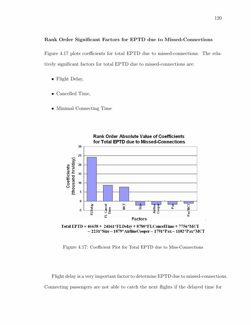
120
Rank Order Significant Factors for EPTD due to Missed-Connections
Figure 4.17 plots coefficients for total EPTD due to missed-connections. The rela-
tively significant factors for total EPTD due to missed-connections are:
• Flight Delay,
• Cancelled Time,
• Minimal Connecting Time
Figure 4.17: Coefficient Plot for Total EPTD due to Miss-Connections
Flight delay is a very important factor to determine EPTD due to missed-connections.
Connecting passengers are not able to catch the next flights if the delayed time for

121
the previous flight is too long to be absorbed by connecting buffer. Both missed
connection passengers and cancelled passengers are disrupted passengers and need
to be re-booked. Cancellation time affects the EPTD due to missed-connections in
a negative way: earlier cancellations (high level) relieve the competition of available
resources between disrupted passengers, and decrease EPTD. Less required time for
passengers walking from one gate to another gives a greater time buffer to absorb
delay brought by the first-leg flight.
An interesting observation is that significant factors and rankings for average
EPTD (min per passenger) are not necessary the same as those for total EPTD
due to missed-connections. Figure 4.18 plots coefficients for average EPTD due
to missed-connections. The relatively significant factors for average EPTD due to
missed-connections are:
• Airline Cooperation,
• Flight Delay,
• Cancelled Time
Total EPTD is a combined result of the number of missed connection passengers
and the average of EPTD due to missed connections. Different factors may have
stronger impacts on average EPTD but not on number of passengers. The effect of
this factor on total EPTD is then determined by the combined effect from both sides.
A good example could be airline cooperation policy. Cooperation between airlines
helps in reducing the average EPTD with no doubt. However, it has nothing to do
with the number of missed connection passengers.

122
Figure 4.18: Coefficient Plot for Average EPTD due to Miss-Connections
In summary, airline cooperation, less flight delay, earlier cancellation time and less
MCT can help reduce both total EPTD and average EPTD due to missed-connections.
Rank Order Significant Factors for EPTD due to Delayed Flights
Figure 4.19 plots coefficients for total EPTD due to delayed flights. The relatively
significant factors affecting total EPTD due to delayed flights are:
• Flight Delay,
• # Passengers
This is a straightforward result, since total EPTD due to delayed flights is only
affected by flight delays and number of passengers loaded on the delayed flights.

123
Figure 4.19: Coefficient Plot for Average EPTD due to Delayed Flights
4.4.4 Sensitivity of Factors
To better understand the magnitude of the impacts of factors on EPTD, total EPTD
for the following experiments are calculated and compared with the total EPTD on
July 6, 2005 (in Table 4.5). Using July 6 as the baseline for vehicle performance, this
analysis determines the sensitivity of Total EPTD to changes in each of the factors.
The analysis gives a snapshot of the sensitivity of the factors. Flight delay has
been proven to be the most significant factor affecting NAS-wide total EPTD. A 15
minute change in flight delay can decreased the total EPTD by 24 percent and save
$2.3 million passenger value of time per day, which will contribute $840 million to
annual save. Note, the listed experiments in Table 4.5 rely on changes in a single

124
factor. Officials, operators and stakeholders of the ATS shall consider changes in a
combination of factors to maximize benefits with relatively low costs for future option
design.
Table 4.5: Sensitivity of the Total EPTD (Delay+Cancel+Missed-Connection) to
Changes in Factors
Changes in FactorsCompared with Total EPTD (320,000 hrs) on
July 6, 2005 (with no change in factors)↓ in Percentage Total EPTD Passenger Value
of Time SavedReduce flight delay by 15
minutes
↓ by 24% 243,000 hrs $2.3 million
Allow airline cooperation ↓ by 12% 283,000 hrs $1.1 millionCancel flights four hours
earlier
↓ by 10% 290,000 hrs $0.9 million
Reduce load factor to
70%
↓ by 8% 296,000 hrs $0.7 million
4.5 Stochastic Passenger Flow Simulation (PFS)
Deterministic PFS is introduced in the previous section. It is a pure conversion from
vehicle performance to passenger performance, and has been proven to be an accurate
conversion within 1% to 2% difference range.
A stochastic PFS is more suitable and valuable for prediction or future option

125
design evaluation purpose. Stochastic factors, such as air time, taxi-in time and
taxi-out time, are set to normal random number generators with different means
and standard deviations. Other significant factors, such as aircraft size, number of
passengers loaded (or load factor), are represented as variables in the stochastic PFS.
Officials, policy makers and researchers can easily change the values of stochastic
factors or variables to represent anticipated changes in the future. The stochastic
PFS provides a flexible simulation environment to conduct experiments outside the
range of historical data.
Note, stochastic and deterministic PFS share the same model structure, but with
different settings of functions and parameters.
4.5.1 Stochastic Factors and Variables
The stochastic factors and variables defined in stochastic PFS are listed as follows:
• Taxi-Out Time:
Category: it is a stochastic factor whose value is given by a normal random
number generator, Normal(µi, σi), where i represents the deparing airport;
Example: taxi-out time for flights departing from ATL fits Normal(µ=20.7
min, σ=10.9 min).
Potential Usage in Specific Scenario: New runway, or more efficient service
of ATC may decrease mean or standard deviation of taxi-out time.
• Air Time:
Category: it is a stochastic factor whose value is given by a normal random
number generator, Normal(µj, σj), where j represents any route.

126
Example: air time for flights on route ATL to BOS fits Normal(µ=123.3 min,
σ=5.6 min).
Potential Usage in Specific Scenario: Usage of new technology or aircrafts
may decrease mean or standard deviation of air time .
• Taxi-In Time:
Category: it is a stochastic factor whose value is given by a normal random
number generator, Normal(µi, σi), where i represents arriving airport.
Category: taxi-in time for flights arriving at ATL fits Normal(µ=10.3 min,
σ=5.9 min).
Potential Usage in Specific Scenario: Better designed taxi-way may de-
crease mean or standard deviation of taxi-in time .
• Minimal Connecting Time (MCT):
Category: it is a variable whose value is given by function MCT(connecting
airport).
Example: MCT for passengers connecting at BOS is set to be 20 minutes.
Potential Usage in Specific Scenario: More efficient gate and terminal
design at an airport may decrease the MCT required for passengers connecting
at this airport.
• # of Passengers:
Category: it is represented as variable “pax” in PaxGroup.
Example: PaxGroup 1‘(“TPA”,“PIT”,96,137,750,888,14,41661,741,96)@+741
indicates there are 96 passengers loaded on a flight with 137 seats flying from
Tampa to Pittsburgh.

127
Potential Usage in Specific Scenario: Increase the value of “pax” variable
for all the PaxGroup coming to a city to represent the increase in passenger
demand.
• Aircraft Size:
Category: it is represented as variable “size” in PaxGroup.
Example: PaxGroup 1‘(“TPA”, “PIT”, 96, 137, 750, 888, 14, 41661, 741,
96)@+741 indicates there are 96 passengers loaded on a flight with 137 seats
flying from Tampa to Pittsburgh.
Potential Usage in Specific Scenario: Increase the value of “size” variable
for all the PaxGroup to/from LGA to represent upgauging aircraft size at LGA.
• Scheduled Departure/Arrival Time:
Category: they are represented as variable “schdeptime” and “scharrtime” in
PaxGroup respectively.
Example: PaxGroup 1‘(“TPA”, “PIT”, 96, 137, 750, 888, 14, 41661, 741,
96)@+741 indicates Flight 41661 is scheduled to depart from Tampa at system
time 750 and arrive at Pittsburgh at system time 888.
Potential Usage in Specific Scenario: Changes in these two variables rep-
resents the time changes in airline schedule.
4.5.2 Simulation Results and Validation: 34-Airport PFS on
July 6 2005
The stochastic PFS has been executed 10 times to obtain stochastic simulation results.
Table 4.6 lists the estimated total and average EPTD for each run. The average and

128
standard deviation for “Total EPTD” on July 6, 2005 are 310,425 hours and 934
hours respectively. The average and standard deviation for “Average EPTD” on July
6, 2005 are 99 minutes and 0.8 minute respectively.
Table 4.6: Stochastic Simulation Results of the Stochastic PFS on July 6, 2005
Run Total EPTD (Delay+ Can-
cel+ MissedConn)
Avg. EPTD (Delay+ Can-
cel+ MissedConn)R1 310,013 hrs 100 minR2 311,281 hrs 99 minR3 310,141 hrs 99 minR4 309,945 hrs 98 minR5 311,169 hrs 98 minR6 309,299 hrs 101 minR7 312,310 hrs 98 minR8 309,316 hrs 98 minR9 310,516 hrs 99 minR10 310258 hrs 99 min
µ 310,425 hrs 99 minσ 934 hrs 0.8 min
Deterministic
PFS
330,834 hrs 103 min
Diff (Determ,
Stoch)
6% 4%
The average “Total EPTD” and the average “Avg. EPTD” of stochastic PFS
are compared with the “Total EPTD” and “Avg. EPTD” of deterministic PFS. The
difference between these two PFS modes are 6% and 4% for “Total EPTD” and “Avg.
EPTD” respectively.
For validation purpose, the simulation results of the stochastic PFS are compared

129
with the baseline. Baseline is the EPTD for July 6 estimated by EPTD algorithm. As
described in the validation section of deterministic PFS (Chapter 4.4.1), only EPTD
due to delayed and cancelled flights are included in the validation process. Table
4.7 lists and compares the simulation results of both the stochastic and deterministic
PFS with baseline.
Table 4.7: Validation of Stochastic PFS
EPTD Al-
gorithm
Deterministic
PFS
Diff1 (Al-
gorithm,
DetermPFS)
Stochastic
PFS
Diff2 (Al-
gorithm,
StochaPFS)Total 306,000 hrs 309,000 hrs 1% 288,000 hrs 6%Average 90 minutes 88 minutes 2% 84 minutes 7%
“Diff1” and “Diff2” in Table 4.2 are calculated as:
• Diff1 (Algorithm, DetermPFS) = absolute value of (Algorithm - DetermPFS)
/ Algorithm * 100,
• Diff2 (Algorithm, StochaPFS) = absolute value of (Algorithm - StochaPFS) /
Algorithm * 100.
The difference between baseline and stochastic PFS is wider than the difference
between baseline and deterministic PFS. This is mostly caused by the value settings
of parameters, such as the mean and standard deviation of stochastic factors. Air
time for flights on a specific route is given by a normal random number generator with
130
historical mean and standard deviation. But in the real world, flights that are already
late for departures intend to make up time by flying faster. As a consequence, flights
with departure delay generally have a smaller air time than others. Better validation
results can be achieved by more detailed definitions and settings , such as providing
different normal random number generators for delayed and on-time departure flights.
Chapter 5: Industrial Applications of Research
The industrial applications and potential users of this research are listed as follows:
1. Traffic Flow Management (Fall 2006): Estimating Airspace Flow Program (AFP)
benefits in support of severe weather for Metron Aviation Inc.
2. FAA Strategy Planning (Spring 2007):
• Trend Analysis for Passenger Trip Delay,
• Estimating Passenger Trip Delay in Year 2010,
• Estimating Passenger Trip Delay for NAS Strategy Simulator
3. Airline Operation Centers
4. Flight Reservation and ticket purchasing
The third and fourth applications are potential users for an Air Transportation
Network Analysis Tool (ATNAT) designed to provide a single source of statistical
information about the performance of the routes, airports and airlines in the air
transportation network. It suggests the most reliable and least-delay-risk route, air-
line, and departure time for passengers based on the passenger’s choice of origin and
destination. Please refer to section 3.3.5 for a detailed introduction for the ATNAT
tool.
131

132
5.1 Traffic Flow Management (Fall 2006)
Airspace Flow Programs (AFPs), introduced operationally by the FAA on June 5,
2006, were used operationally on 19 days in June through September as an alter-
native to Ground Delay Programs (GDPs) in support of Severe Weather Avoidance
Procedures (SWAP). GDP was originally developed to address the need to efficiently
meter airport arrival flows during periods of reduced airport arrival capacity. It delays
inbound flights on the ground prior to departure. But when GDP is used in support
of SWAP, it is “inefficient, ineffective and inequitable” (Libby et al., 2005):
1. Inefficient: most of the delay is applied to flights that are not part of the
problem.
2. Ineffective: control only a fraction of the flights in the problem area.
3. Inequitable: only flights bound for large airports are ever affected.
Figure 5.1 illustrate an example of GDP in support of SWAP. A line of thunder-
storms (shown as the FCA in the figure) moved across the eastern U.S. on July 7,
2004. Ten airports were issued GDP and 86,654 minutes of ground delay was im-
posed. However, (a) 60 percent of flights that entered Flow Constrained Area (FCA)
were uncontrolled by SWAP GDPs, and (b)80 percent of GDP-controlled flights did
not traverse FCA.

133
Figure 5.1: Example of GDP in Support of SWAP (?)
The Collaborative Decision Making (CDM) community has recognized these lim-
itations and is seeking a method to systematically manage demand at a constrained
en route resource by identifying the flights that are expected to use that resource and
holding them on the ground until the airborne capacity to deal with them is available.
This is the precise function that the Airspace Flow Program (AFP) is designed to
provide (Libby et al., 2005).
In the first operational analysis and performance assessment (Metron AFP Report
I, 2006), Metron Aviation Inc. reported initial findings on AFP usage, compliance,
equity, and initial estimates of savings realized in using AFPs instead of SWAP GDPs.
This analysis focused on flight-based analysis. In the second AFP deliverable to the

134
FAA, Metron Aviation Inc. looked at the AFP benefits from the flying public’s view
instead of a flight-based operational view. They continued to look at how AFP tech-
nology and procedures were used and what progress was made in meeting expectations
of reduced delay and passenger disruption. The report to FAA is organized into four
sections, and the passenger delay estimating algorithm is applied in the third section
“Passenger Delay Analysis.”
1. Delay Comparison
2. Detailed look at AFP Usage (by Danyi Wang)
3. Passenger Delay Analysis (by Danyi Wang)
4. Recommendations
Estimated Passenger Trip Delay (EPTD) is calculated for the 19 AFP days in 2006
and the 16 GDPs in support of SWAP days in 2005. Results prove that using AFP
has advantages over using GDP in support of SWAP. AFPs affected 24 percent less
delayed flights and 78 percent less cancelled flights than GDPs in support of SWAP.
It results in 50 percent less passenger trip delays and avoids millions of daily loss
in passenger value of time. Detailed analysis and statistics are available in Metron’s
reports, but will not be exposed in this thesis.
5.2 FAA NAS Strategy Simulator (Spring 2007)
The NAS Strategy Simulator (NSS) was developed by Ventana Systems in conjunction
with NEXTOR (nextor.org) for the FAA. The simulator is a dynamical system model
of the NAS designed to understand the interactions between three sectors: Passengers

135
and Shippers, Airlines, and system of airports and Air Traffic Control (Sherry et
al., 2003). The Center of Air Transportation Systems Research conduct a study to
estimate the passenger trip delays in 2010 and develop an NSS module to estimate
passenger trip delays given anticipated changes in the future.
5.2.1 EPTD in 2010
In order to estimate passenger trip delays in 2010, we have
1. forcasted daily flight schedule in 2010 given by the FAA,
2. estimated load factor in 2010 (88%),
3. assumed increase in flight arrival delay in 2010,
4. estimated flight cancellation rate in 2010 (3.3%)
The 88% load factor is estimated by continuing the increase trend of load factor
after 2006 (see Figure 5.2)
Similarly, percentage of delayed flights from January 2002 to May 2007 is depicted
in Figure 5.3.
According to the trend, the percentage of delayed flights will reach 30 percent
in 2010. The distribution of flight arrival delay on a specific route i is a lognormal
distribution with µi and σi. The arrival delay for each flight in the model is generated
by the corresponding lognormal random number generator for that specific route. We
assume both µ and σ for each route will be increased by 20 percent until 2010 to
achieve “30 percent delayed flights” in 2010.
Figure 5.4 illustrates the regression between the percentage of cancelled flights and
the percentage of delayed flights from 2002 to 2007. Data before 9/11 is excluded,
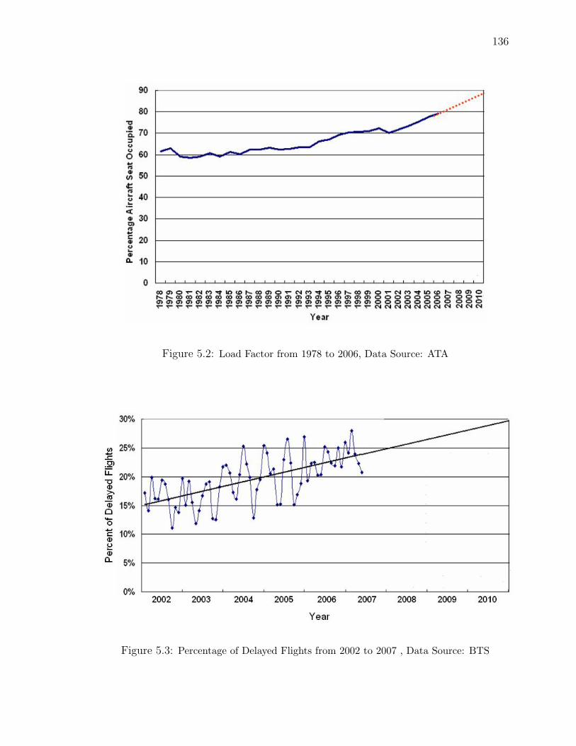
136
Figure 5.2: Load Factor from 1978 to 2006, Data Source: ATA
Figure 5.3: Percentage of Delayed Flights from 2002 to 2007 , Data Source: BTS

137
since position and shape of the regression curve has changed after 9/11 due to a
structural shift of the system (Wang et al., 2006), (Tam and Hansman, 2003). The
estimated flight cancellation rate in 2010 is 3.3 percent.
Figure 5.4: Correlations Between Percentage of Delayed Flights and Percentage of Can-
celled Flights, Data Source: BTS
As shown in Figure 5.5, the EPTD estimation process consists of two “black
boxes.” Given individual flight schedules, estimated changes in flight delay, estimated
cancellation rates, and estimated load factors, flight performance is first estimated
in black box 1. 3.3 percent of scheduled flights are randomly selected as cancelled
flights, and the 96.7 percent of non-cancelled flights are updated with “arrival de-
lay” generated by lognormal random number generators. Black box 2 is responsible
for calculating passenger trip delays given flight performance data. The underlying

138
algorithm of black box 2 is the EPTD algorithm.
Figure 5.5: Estimation Passenger Trip delay in 2010
Comparing performance in 2005 with performance in 2010, the 22 percent increase
in daily scheduled flights generated 175 percent increase in total EPTD. As shown
in Table 5.1, the 22 percent increase in daily scheduled had a strong impact on both
flight performance and passenger performance, but passenger performance is much
more sensitive:
1. Flight Performance: 212 percent increase in daily scheduled flight resulted in
• 75 percent more delayed flights, and
• 127 percent more cancelled flights.
2. Passenger Performance: 21 percent increase in daily scheduled flight results in

139
• 195 percent more total EPTD,
• 140 percent more EPTD due to delayed flights,
• 278 percent more EPTD due to cancelled flights,
• 14.5 percent increase in average EPTD due to delayed flights,
• 25.1 percent increase in average EPTD due to cancelled flights.
The 21 percent increase in daily scheduled flights resulted in 75 percent and 127
percent increase in delayed and cancelled flights respectively. The 75 percent increase
in delayed flights generated 140 percent increase in EPTD due to delayed flights.
Similarly, the 127 percent increase in cancelled flights generated 278 percent increase
in EPTD due to cancelled flights. Both increases in EPTD are almost twice the
increase in flights.
Figure 3.12 shows that 2000 generated the highest annual total EPTD (180 million
hours) so far. Table 5.2 lists and compares the average daily performance in 2000
and 2010.
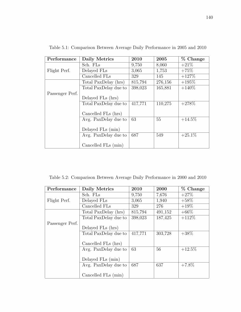
140
Table 5.1: Comparison Between Average Daily Performance in 2005 and 2010
Performance Daily Metrics 2010 2005 % Change
Flight Perf.Sch. FLs 9,750 8,060 +21%Delayed FLs 3,065 1,753 +75%Cancelled FLs 329 145 +127%
Passenger Perf.
Total PaxDelay (hrs) 815,794 276,156 +195%Total PaxDelay due to
Delayed FLs (hrs)
398,023 165,881 +140%
Total PaxDelay due to
Cancelled FLs (hrs)
417,771 110,275 +278%
Avg. PaxDelay due to
Delayed FLs (min)
63 55 +14.5%
Avg. PaxDelay due to
Cancelled FLs (min)
687 549 +25.1%
Table 5.2: Comparison Between Average Daily Performance in 2000 and 2010
Performance Daily Metrics 2010 2000 % Change
Flight Perf.Sch. FLs 9,750 7,676 +27%Delayed FLs 3,065 1,940 +58%Cancelled FLs 329 276 +19%
Passenger Perf.
Total PaxDelay (hrs) 815,794 491,152 +66%Total PaxDelay due to
Delayed FLs (hrs)
398,023 187,425 +112%
Total PaxDelay due to
Cancelled FLs (hrs)
417,771 303,728 +38%
Avg. PaxDelay due to
Delayed FLs (min)
63 56 +12.5%
Avg. PaxDelay due to
Cancelled FLs (min)
687 637 +7.8%

141
According to the prediction, both flight and passenger performance in 2010 will
be worse than any historical year.
One of the assumption of this research is that the ATS capacity remains at the
same level of 2005 in 2010.
The analysis confirms once again that (1) EPTD increases dramatically with the
number of scheduled flights in the system, and (2) passenger performance is more
sensitive to the changes than flight performance, especially when the demand is very
close to or more than the system capacity.
5.2.2 EPTD Module for NSS
A system-level NSS module was developed to estimate passenger trip delays given
anticipated changes. Figure 5.6 depicts the module structure in the NAS strategy
simulator. In this module, year 2006 is used as a baseline in the module. M1:
impact of load factor on passenger trip delay, and M2: impacts of flight frequency
on passenger trip delay are the major factors affecting PaxDelay in the NAS. They
are calculated and compared with those in the baseline. If M1 and M2 in year X
enlarged the impact by x%, then the corresponding average passenger trip delay will
be increased by x%.
Figure 5.7 lists all the equations used behind the module.

142
Figure 5.6: Estimating Passenger Trip Delay Module for NSS

143
Fig
ure
5.7:
Equ
atio
nsU
sed
inth
eN
SSM
odul
e

Chapter 6: Conclusions and Future Work
The goal of Air Transportation Services is to make a safe, affordable, and convenient
transport service for passengers and cargo. As a consequence, the top level perfor-
mance measures of the ATS should include the trip delays experienced by airline
passengers. Passenger-based metrics, together with flight-based metrics can give a
more accurate and complete description of the ATS performance.
The results reflect the asymmetric and unique passenger trip on-time performance
and capture the complexity and significance of the impact of a small set of cancelled
flights and missed connections on passenger trip delays. Note, all the statistics listed
in this chapter are based on data in 2006.
6.1 Disproportionately High EPTD due to Can-
celled Flights and Missed Connections
The results indicate that the distribution of passenger trip delays is a heavily skewed
distribution with a long tail. Passenger trip delay does not distribute evenly through
the passengers: passengers scheduled on cancelled flights or missed connections only
account for 3 percent of the total enplanements, but they generated 45 percent of
total EPTD and experienced a high average delay of 382 minutes (roughly 6 and half
hours).
144
145
6.2 Asymmetric Behavior of EPTD in terms of
Routes, Airports and Months
Seventeen percent of the 1030 routes between OEP 35 airports generated 50 percent
of the total EPTD. This illustrates the significantly higher number of trip delays ab-
sorbed by less than 1/5 of the routes. An interesting finding is that routes between
New York metropolis and Washington D.C. metropolis have the highest average pas-
senger trip delays in the system.
Nine of the 35 OEP airports generated 50 percent of the EPTD. The EPTD
by airport is spread more evenly than the EPTD by routes, but still impacts some
airports significantly more than others (e.g. ORD, ATL, DEN, EWR and LGA)
For months, the highest-ranked five months: December, July, June, February and
October, absorbed 51 percent of total EPTD. The rank order in terms of month is
not always the same. For example, the highest-ranked four months which absorbed
50 percent of total EPTD in 2004 are: September, August, July and December.
6.3 Flight-Based and Passenger-Based Metrics
Flight-based metrics have been proven to be a poor proxy for passenger on-time
experience (Bratu, 2003), (Bratu and Barnhart, 2005), (Ball et al., 2006). The asym-
metric absorption of delays by different groups of passengers indicates that care must
be used in the selection of system-wide metrics. This type of metric can unintention-
ally distort the actual performance of the system and effectively “hide” explanatory
and diagnostic system behavior. The “percentage” and “count” flight-based metrics

146
do not reflect the degree of delay in excess of 15 minutes or the passenger travel expe-
rience. For example, a flight with 16 minutes delay and a flight with 60 minutes delay
results in the same flight-based on-time performance when “percentage” or “count”
metrics are used. Similarly, an evening cancelled flight with 300 passengers might
generate a large number of passenger trip delays, but it is measured to be the same
as an early cancelled flight with 50 passengers when flight-based metrics are used,
since both account as “one cancelled flight”. One way to capture the passenger expe-
rience in a metric for the performance of the air transportation system is to compute
the EPTD on a daily, monthly or annual basis. This metric, computed by running the
algorithm described in this thesis, could serve as an indicator of passenger customer
satisfaction of the performance of the system as a whole.
6.4 Accuracy of EPTD
Both flight operational data and passenger(seat) data are needed for the computation
of Estimated Passenger Trip Delay (EPTD). Since the passenger data (such as pas-
sengers loaded, aircraft size, load factor) for a given flight is not publicly available, the
algorithm used in this analysis, uses the average value for the passenger factors over
the period of analysis. This estimate assumes that values of passenger factors (e.g.
aircraft size, number of passengers and empty seats) are normally distributed around
a mean that reflects the average value for all flights (Chapter 3.2). For the purpose of
the analyzing of the system-level performance, this assumption is satisfactory. Based
on the stochastic simulation runs, the model prodiction is within approximately 10%
of expected actual value.

147
6.5 Dealing with the Cancelled Flight Phenomenon
Contrary to popular belief, there are no federal requirements, and the airlines are not
under any legal obligation, to guarantee their schedules (DOT, 2006). Furthermore,
airlines are not required to compensate passengers whose flights are delayed or can-
celed. As a result regulation of airline cancellation practices is left to the market-based
notion that consumers will “vote with their pocket-book” and not patronize airlines
that tend to leave passengers stranded. This mechanism is not entirely efficient.
In general, the cancellation of a single flight is not an isolated event for the air-
line. Depending on the aircraft routing, a cancelled flight can result in a ripple of
flight cancellations throughout the day, causing missed connections and disruptions
at upstream and downstream airports. To minimize the impact to the overall airline
schedule, airlines often choose to cancel several legs to avoid having to ferry aircraft
to catch up to the aircraft routing. A cancellation cycle is a sequence of legs in a
rotation in which the first leg departs from the same airport at which the last leg.
These practices are not well understood and have been the widely reported in the
research literature. In particular the impact of “traffic flow initiatives” on airline
cancellation and delay practices has not been studied (Sherry et al., 2007).
Flight cancellation is a complicated disruption to passengers since it has a stronger
impact on passenger trip delay than flight delay does. To mitigate the effects of flight
cancellation on passenger trip time, airlines could either provide redundant resources
or reduce cancellation. The redundant resources include more empty seats, lower
load factor, higher flight frequency, backup aircraft and flight crew. These redundant
resources ensure the flexibility of re-booking process when disruptions happen. But

148
on the other hand they increase airline costs and lower airline efficiency.
Due to the cost-cutting strategy used by most of today’s airlines, load factor is
increasing rapidly. Over booking causes more disrupted passenger, and less empty
seats make the re-booking of disrupted passengers even harder. Passenger trip de-
lay increases exponentially with the increase of the load factor (Bratu, 2003). The
complexity of impacts of cancelled flights on passenger trip time has changed with
the changes in airline market strategy and recover policy. The significant factors
control these strategies and policies need to be included in the simulation model for
predictions in the future.
6.6 Passenger Perspective
Under this system passengers must treat trip time as a stochastic phenomenon that
can be assigned a probability of occurrence, but cannot be avoided entirely in any
systematic manner. As described in this paper, airports/routes are factors that deter-
mine the performance of the system. Simple strategies can be used by the passenger
to reduce the probability of occurrence such as choice of departure airport and choice
of route. For example, for trip from Washington, D.C. to Chicago, during the period
analyzed in this paper, the flights from Washington Reagan International Airport
(DCA) to Midway (MDW) had a 5 percent probability of more than one hour delay,
whereas the flight from DCA to Chicago O’Hare had 12 percent of probability of more
than one hour delay. Future work in this area involves the development of metrics
useful to passengers such as time-of-day, day-of-week, monthly, and annual trends in
airport and route performance. Also analysis of likelihood of cancellation or EPTD
for specific flights could be provided as an aid to consumers (Wang et al., 2007 A).

149
6.7 Consumer Protection for Airline Travelers
The traditional view of consumer protection - the one adopted by the Department of
Transportation - is to provide a comparison of flight-based services provided by the
airlines to the passengers. This approach is based on the premise that the difference
in service is derived only by the performance of the airlines. This view of consumer
protection fails to recognize the effect of the integrated system, composed of airlines,
airports, air traffic control, employment contracts, government funding systems, etc.
This data illustrates the importance of consumer protection against the system (not
just the enterprise).
Passenger based performance metrics are designed for airline travel consumer pro-
tection and capture the integrated performance of all the agents. These metrics will
enable passengers to make choices regarding the air entire transportation system, not
just the airlines.
It is recognized that these metrics represent “holistic” metrics of the performance
of the “integrated” air transportation system. Improving these metrics is beyond the
ability of individual enterprises in the supply chain (e.g. airlines, Air Traffic Control,
airports, etc.). Improvement demands an integrated and cooperative solution. In
addition, the data should be presented in a way to enable comparison of routes
between markets.
6.8 Recommendations for Future Work
We identify the following potential ground for future work:

150
DOE with Non-linear Stochastic Runs
Trend analysis in Chapter 3.3.2 showed the growth of air transportation traffic has
slowed down and leveled off in 2006. This trend indicates a non-linear relationship
between significant factors affecting the system performance. Instead of having a lin-
ear (two-level) fractional factorial design for the deterministic PFS (in Chapter 4.4.2),
a non-linear (three-level) fractional factorial experiment with interactions should be
designed and applied on the stochastic PFS.
More Detailed Passenger and Seat Information
The EPTD algorithm is based on aggregated passenger and seat information from the
T-100* database. The aggregated data limits the detail level of investigation, since
it assumes that flights in peak hours have the same load factor as flights in non-peak
hours. For the purpose of the analyzing air transportation system performance, this
assumption is satisfactory. Future work is planned to investigate actual passenger
enplanements and aircraft size from proprietary airline data.
More Detailed Parameter Setting in PFS
As explained in Chapter 4, more accurate simulation results can be achieved by pro-
viding more detailed definitions of parameters and distributions, such as using two
random number generators to generate air time for flights with departure delay and
flights without departure delay. The current stochastic passenger flow simulation
model distinguishes passengers and flights in terms of airport, route and carrier. We
recommend more meticulous differentiation of PaxGroup: not only in terms airport,

151
route and carrier, but also in terms of time of day, peak/non-peak hour, with depde-
lay/wo depdelay, etc.
Adding Ticket Price as a New Passenger-Based Metric Representing Costs
The Airline Origin and Destination Survey (DB1B) Market Database contains a 10
percent sample of airline tickets from reporting carriers. Market fare is one of the fields
provided by the DB1B, which can be used as average ticket price paid by passengers.
A new passenger-based metric could be developed from DB1B database presenting
average market value (or cost to passengers) for a specific route operated by a specific
airline. This metric, combined with EPTD metric, can tell the quality of service
passengers received based on the price they paid for the service. In other words,
the combination of EPTD metric and market value metric provides a cost/benefit
analysis for passenger trips.
Build Java GUI for PFS
The passenger flow model is developed in CPN Tools, which is a GUI tool for editing,
simulating and analyzing Colored Petri Nets. Dr. Abbas Zaidi and his students in
Electronic and Computer Engineering Department of George Mason University are
developing a java tool for CPN Tools. The java tool hides CPN model in a black box
and allows general users to modify inputs and parameters without knowing petri nets.
It also helps model developers protect the core model from unexpected modification,
or even insulate the core model from irrelevant people.

152
Bibliography

153
Bibliography
(AOTP) The Bureau of Transportation and Statistics, Airline On-Time Performance Data.
http://www.transtats.bts.gov/Tables.asp?DB_ID=120&DB_Name=Airline%20OnTime%20Performance%20Data&DB_Short_ Name=On-Time
(ASPM) The Federal Aviation Administration, Aviation System Performance Metrics (ASPM) Database, http://www.apo.data.faa.gov/aspm/entryASPM.asp
(ASTA) American Society of Travel Agents, Air Traveler's Bill of Rights http://www.astanet.com/govaffairs/trav_rights.asp
The ATA Economic Annual Report(ATA Report) The Airline Transport Association, http://www.airlines.org/economics/review_and_outlook/ annual+reports.htm
(CNS/ATM Report, 1999) Air Traffic Services Performance Focus Group (ATSP FG) And NS / ATM focused Team (C/AFT) (1999), Airline Metric Concepts for Evaluating Air Traffic Service Performance, CNS / ATM focused Team Report, February 1999.
(Ball et al., 2006) Ball, M., Lovell, D., Mukherjee, A. Subramanian, B.(2005), Analysis of Passenger Delays: developing a passenger delay metric, NEXTOR NAS Performance Metrics Conference, ASilomar, CA. March 2006.
(Barnhart and Bratu) Barnhart, C. and Bratu, S. (2004), Airline Passenger Delays, Solan Industry Centers Annual Conference, April 2004, Atlanta, GA.
(Beatty et al., 1998) R. Beatty, R. Hsu, L. Berry and J. Rome (1998), Preliminary Evaluation of Flight Delay Propagation Through and Airline Schedule, the 2nd USA/Europe Air Traffic Management R&D Seminar, Orlando, Florida, 1998.
(Belobaba, 1987) Belobaba, P. (1987), Air Travel Demand and Airline Seat Inventory Management, PhD Dissertation in Aeronautics and Astronautics,

154
Supervisor: Robert Simpson, Massachusetts Institute of Technology, Cambridge, MA.
(Bhadra and Texter, 2005) Bhadra, D., Texter, P. (2005), Airline Networks An Econometric Framework to Analyze Domestic US Air Travel, Journal of Transportation and Statistics, Vol. 7 Number 1.
(Blom et al., 2000) Blom, H., Daams J. and Nijhuis, H.(2000), Human Cognition Modeling in Air Traffic Management Safety Assessment, the Fifth Probabilistic Safety Assessment and Management Conference, Osaka, Japan
(Bolczak and Ho man, 1997) Bolczak, C., Hoffman J. (1997),AIS-BN: National Airspace System Performance Measurement, MITRE technical report MTR97W0000035.
(Boswell and Evans, 1997) Boswell, S. and Evans, J. (1997), Analysis of Downstream Impacts of Air Traffic Delay, Project Report ATC - 257, MIT Lincoln Laboratory, Cambridge, MA. 1997.
(Bowen and Headley, 2006) Bowen, B. and Headley, D. (2006) Airline Quality Rating: http://www.aqr.aero/
(Bratu, 2003) Bratu, S. (2003), Airline Passenger On- Time Schedule Reliability: Analysis, Algorithms and Optimizaiton Decision Models, Ph.D Thesis, Supervisor: Cythia Barnhart, Massachusetts Institute of Technology, Cambridge, MA.
(Bratu and Barnhart, 2005) Bratu, S., Barnhart, C. (2005), An Analysis of Passenger Delays Using Flight Operations and Passenger Booking Data, Air Traffic Control Quarterly, Number 1, Volume 13.
(Bratu and Barnhart, 2006) Bratu, S. and Barnhart, C. (2006), Flight Operations Recovery: New Approaches Considering Passenger Recovery, Journal of Scheduling, Volume 9, issue 3, Page: 273-298, June 2006
(Breunig et al., 2003) Breunig, T., Bradford, S. and Liang, D. (2003), Standardizing Performance Metrics, the 5th USA / Europe Air Traffic Management R&D Seminar, Budapest, Hungary, June 2003
(CAAP 1999) Canadian Association of Airline Passengers (1999), Canadian Association of Airline Passengers and the Airline Passengers Bill of Rights. http://www.cbc.ca/consumers/market/files/travel/air_complaints/bill_of_rights.pdf

155
(Castelain and Mesghouni, 2002) Castelain, E., Mesghouni, K (2002), Regulation of a public transport network with consideration of the passenger flow modeling of the system with high-level Petri nets, Systems, Man and Cybernetics, IEEE International Conference on, Volume 6, 6-9 Oct. 2002 Page(s): 5 pp. vol.6
(Cherniavsky and Abrahamsen, 2000) Cherniavsky, E. and Abrahamsen, T. (2000) , Aviation System Performance Metrics:
MPReport:Development SystemAviationAdvancedCenter for Airport Utilization, MITRE
00W0000090, Project No.: 02001207-20, April 2000
(Consumers Union 2001) Consumers Union (2001), Consumers Union Calls on Congress to Address Primptly Reid Bills on Airline Passenger Rights, competitionhttp://www.consumersunion.org/other/reiddc101.htm.
(DB1B) The Bureau of Transportation and Statistics, Airline Origin And Destination Survey (DB1B) Data http://www.transtats.bts.gov/Tables.asp?DB_ID=125&DB_Name=Airline%20o rigin%20and%20Destination%20Survey%20%28DB1B%29&DB_Short_Name =Ori gin%20and%20Destination% 20Survey
(Double et al., 2006) Double, N., Brennan, M., Arora, N., Ermatinger, C. and Clover S. (2006), Simulation and Operational Analysis of Airspace Flow Programs for Traffic Flow Management, 6th AIAA Aviation Technology, Integration and Operations Conference, September 2006, Wichita, Kansas.
(Donohue and Zellweger, 2001) Donohue, G., Zellweger, A. (2001). Air Transportation Systems Engineering, American Institute of Aeronautics & Astronautics (AIAA), Herndon, VA.
(Donohue and Shaver, 2008) Donohue, G. and Shaver, R. (2008), Prisoners, Sheepand Autocrats: A Tale of United States Air Transportation, to be published, RAND Corporation, Arlington VA.
(DOT) Department of Transportation, Air Travel Consumer Report 1998- 2006.http://airconsumer.ost.dot.gov/reports/index.htm
(Eurocontrol) Eurocontrol Performance Review Commission (2006), Performance Review Report: An Assessment of Air Traffic Management in Europe During the Calendar Year 2006 http://www.eurocontrol.int/prc/public/standard_page/doc_ prr.html

156
The Federal Aviation Administration, FAA Flight Plan Performance Report(FAA) http://www.faa.gov/about/plans_reports/Performance/
(FAA, 1997) Federal Aviation Administration (1997), Treatment of Values of Passenger Time in Air Travel, http://www.fly.faa.gov/Products/Information/information.html
(FAA, 2004) Federal Aviation Administration (2004), Airport Capacity Benchmark Report 2004 http://www.faa.gov/about/office_org/headquarters_offices/ato/publications/bench
(Foreman and Shea, 1999) Foreman, S. and Shea, D. (1999), Publication of Information and Market Response: The Case of Airline on Time Performance Reports, Review of Industrial Organization, Volume 14, Number 2, March 1999 , pp. 147-162 (16)
(GOTP) The Bureau of Transportation and Statistics, On-Time Performance - Flight Delays at a Glance, http://www.transtats.bts.gov/HomeDrillChart.asp?URL_SelectYear=2005&URL_SelectMonth=4&URL_Time=1&URL_ Selection=1
(Guimera and Amaral, 2004) Guimera, R. and Amaral, L. (2004), Modeling the world - wide airport network, The European Physical Journal B -Condensed Matter and Complex Systems, Volume 38, Number 2/March, 2004.
(Heskett et al., 1994) Heskett, J., Jones, T., Loveman, G., Sasser, W. and Schlesinger, L. (1994), Putting the Service-Profit Chain to Work, Harvard Business Review, March-April 1994, 164-174.
(Hielscher et al., 1998) Hielscher, W., Urbszat, L., Reinke, C. and Kluge, W. (1998), On Modelling Train Tra c in a Model Train System, the First Work- shop and Tutorial on Practical Use of Coloured Petri Nets and Design/CPN, June 8-9, 1998, Aarhus, Denmark.
(Holmes and Scott, 2004) Holmes, B. and Scott, J. (2004), Transportation Network Topologies, in Proceedings of the Fourth Integrated Communications, Navigation, and Surveillance (ICNS) Conference and Workshop, Hyatt Fair Lakes
Hotel, Fairfax, VA
(Hsiao and Hansen, 2006) Hsiao, C. and Hansen, M. (2006), An Econometric Analysis of U.S. Airline Flight Delays with Time-of-Day Effects, the 85th Transportation

157
Research Board (TRB) conference, Washington D.C. January 2006
(Jansen et al., 1998) Jansen, L., Meyer, M. and Schnieder, E. (1998), Technical Issues in Modelling the European Train Control System (ETCS) Using Colored Petri Nets and the Design/CPN Tools, in Proceedings of the 1st CPN Workshop, DAIMI PB 532, pages 103-115
(Janusewski, 2002) Janusewski, R. (2002), Economic analysis for Laguardia, MIT Global Industry Program:ongoing Research, Industry Structure and competition
(JDP) JD Power and Association, Airport Passenger Satisfaction Study, Westlake Village CA.
http://www.jdpower.com/corporate/news/releases/pressrelease.aspx?id=200707
(Karlssona et al., 2004) Karlssona, J., Odonib, A. and Yamanaka, S. (2004), The impact of infrastructure related taxes and fees on domestic airline fares in the US, Journal of Air Transport Management, Volume 10 page 285-293.
(Kristensen et al., 1998) Kristensen, L., Christensen, S. and Jensen, K. (1998), the practitioner's guide to Coloured Petri Nets, International Journal on Software Tools for Technology, pg 98 - pg 132, Volume 2, Number 2 / December, 1998
(Kovace et al., 2004) Kovace, A., Nemeth, E. and Hangos, K. (2004) Colored Petri Net Model of a Simple Runway, Technical Report of the Systems and Control Lab SCL-001/2004. Budapest, MTA SZTAKI, 2004.
(Laskey et al., 2006) K. Laskey , N. Xu and C. H. Chen (2006), Propagation of Delays in the National Airspace System (NAS), the 22nd Conference on Uncertainty in Artificial Intelligence, MIT, Cambridge, July 2006.
(Libby et al., 2005) Libby, M., Buckner, J., and Brennan, M. (2005), Operational Concept for Airspace Flow Programs (AFP) Version 1, FAA Air
Traffic Organization System Operations Services Report, 2005 http://cdm.fly.faa.gov/Workgroups/flow_eval/Operational%20Concept%20for %20Airspace%20Flow%20Programs.doc
(Metron AFP Report I, 2006) Clover, S., Ermatinger, C., Gallus, D. and Myers, T. (2006), Airspace Flow Programs Operations Report: Application of AFPs for
Congestion Management during Severe Weather Events, FAA Deliverable, Metron Aviation, September 2006.

158
(Metron AFP Report II, 2006) Clover, S., Brennan, M. and Wang, D. 2006 ), Airspace Flow Programs Operations Report: Future Analysis of 2006 AFPs and 2005 SWAP-GDPs, FAA Deliverable, Metron Aviation, November 2006.
(Ostrt and Strong, 2006) Oster,C., Strong, J. (2006), Evolution of U.S. Domestic Airline Route Networks Since 1990, The 85th Transportation Research Board (TRB) Conference, Washington D.C. January 2006.
(Perdu, 1997) Perdu, D. (1997), Distributed Process Coordination in Adaptive Comma- and and Control Teams, PhD Dissertation, George Mason University, Fairfax, VA
(Perkusich, 1999) Perkusich, A. (1999), Design and Animation of Coloured Petri Nets Models for Tra c Signals, The 2nd Workshop and Tutorial on Practical Use of Coloured Petri Nets and Design/CPN, June 8-9, 1998, Aarhus, Denmark.
Post W. (2005), Metrics and Performance Management, the 6th USA/-(Post, 2005) Europe ATM R&D Seminar, Baltimore, Maryland, July 2005.
(Riedel and Clarke, 2005) Riedel, R. and Clarke, J. (2005), Airline Operations Feedback Control with KPIs, in Proceeding of AGIFORS Airline Operations 2005 Conference Mainz, Germany.
(Sarmadi, 2004) Sarmadi, S. (2004), Minimizing airline passenger delay through inte- grated fight scheduling and aircraft routing, M.S Thesis, Massachusetts Institute of Technology, Cambridge, MA.
(Shavel, 2000) Shavel, Z. (2000), The Effects of Schedule Disruptions on the Economics of Airline Operations, the 3rd USA/Europe Air Traffic Management R&D Seminar Napoli.
(Sherry et al., 2003) Sherry, L., Mezhepoglu, B. and Goldner, D. (2003), Overview of the FAA's NAS Strategy Simulator, NASA - Integrated CNS Conference. May, 2005.
(Sherry et al., 2007) Sherry, L., Wang, D. and Donohue G. (2007), Air Travel Consumer Protection: A Metric for Passenger On- Time Performance, Journal of Transportation Research Board, to be published, 2007.
(Shaw, 1999) Shaw, A. (1999), A Guide to Performance Measurement and Non- Financial Indicators, Mattison Public Relations, the Foundation For Performance Measurement.
http://www.fpm.com/journal/mattison.htm

159
(Suzuki, 2000) Suzuki, Y. (2000), The Relationship Between On-Time Performance and Airline Market Share: A New Approach, Transportation Research Part E: Logistics and Transportation Review, Volume 36, Number 2, June 2000 , pp. 139-154(16)
(T100) The Bureau of Transportation and Statistics, Form 41 Traffic T-100 Domestic Segment Data
http://www.transtats.bts.gov/Tables.asp?DB_ID=110&DB_Name=Air%20Carrier%20Statistics%20%28Form%2041%20Traffic%29&DB_Short_Name=Air%20Carriers
(Tam and Hansman, 2003) Tam, R. and Hansman, R. (2003), Analysis of the Dynamics of the US Commercial Air Transportation System, Report No. ICAT-2003-2, MIT International Center for Air Transportation, Department of Aeronautics and Astronautics, Massachusetts Institute of Technology, Cambridge, MA 02139.
(Theis, 2005) Theis, G. (2005), How Relevant is Elapsed Time in Passenger Airline Choice?, Industry Advisory Board / Airline Industry Consortium Joint Meeting, Nov 2005, Massachusetts Institute of Technology, Cam- bridge, MA 02139
(Travel Insider, 2005) The travel insider, We Need an Airline Passenger Bill of Rights http://www.thetravelinsider.info/2005/ weneedapassengerbillofrights.htm
(Turki et al., 2003) Turki, A., Grunder, O. and Elmoudni, A. (2003), Periodic Event Scheduling Based On Controlled Stochastic Peti Net, System Theory, 2003. in Proceedings of the 35th Southeastern Symposium on, 16-18 March 2003 Page(s) :386 - 391
(Turki et al., 2002) Turki, A., Grunder, O. and Moudni, A. (2002), Public transportation systems modeling and analysis based on a new Petri net approach, in Proceedings of the 2nd IEEE International Conference on Systems, Man and Cybernetics (SMC'02), October 6-9, 2002, Hammamet, Tunisia, Volume 5. October 2002
(Vigneau, 2003) Vigneau, W. (2003), Flight Delay Propagation: Synthesis of the Study,EUROCONTROL 2003, EEC Note, Internal code: EEC-2003- 018.
(Wagenhals, 2000) Wagenhals, L. (2000), Course of Action Development and Evaluation Using Discrete Event System Models of Influence Nets, PhD Dissertation, George Mason University, Fairfax, VA

160
(Wang et al., 1999) Wang, J., Jin, C. and Deng, Y. (1999), Performance Analysis of Traffic Networks Based on Stochastic Timed Petri Net Models, the 5th IEEE International Conference on Engineering of Complex Computer Systems, October 18-21, 1999 Las Vegas, Nevada, USA
(Wang et al., 2003) Wang, P., Schaefer, L. and Wojcik, L. (2003), Flight Connections and Their Impacts on Delay Propagation, in Proceedings of the 22nd Digital Avionics Systems Conference. Volume 1, 12-16.
(Wang et al., 2006) Wang, D., Mezhipoglu, B., Drexler, J. and Sherry, L. (2006), Estimating Economic Loss Due to a Shortfall in Capacity of the NAS, the 84th Transportation Research Board (TRB) Annual Meeting, January 2006, Washington, D.C.
(Wang et al., 2007 A) Wang, D., Sherry, L. and Donohue, G. (2007), Trend Analysis of Airline Passenger Trip Delays, the 86th Transportation Research Board (TRB) Annual Meeting, January 2007, Washington, D.C.
(Wang et al., 2007 B) Wang, D., Sherry, L. and Donohue, G. (submitted 2007), System Analysis of Flight and Passenger Trip Delays in the National Airspace System, the 26th Digital Avionics Systems Conference, October 2007.
(Welch and Lloyd, 2001) Welch, J. and Lloyd, R. (2001), Estimating Airport System Delay Performance, the 4th USA/Europe Air Traffic Management R & D Seminar, Santa Fe, December 2001
(Williams et al., 2004) Williams, A., Bradford, S., Post, W. and Pomeret, J. (2004), Common Metrics Framework for ATM Performance Assessment and Monitoring, in Proceedings of Digital Avionics Systems Conference, 2004, the 23rd Volume 1, 24-28 Page(s):2.C.4 - 21-13 Vol.1, Oct. 2004
(Xu et al., 2005) Xu, N., Donohue, D., Laskey, K and Chen, C. H (2005), Estimation of Delay Propagation in the NAS Using Bayesian Networks, in Proceedings of Air Traffic Management Seminar, Baltimore, MD, June 2005
(Xu et al., 2007) Xu, N., Donohue, G., Laskey, K., Chen, C.H., Williams S. and Sherry L. (2007), Bayesian Network Analysis of Flight Delays, the 86th Transportation Research Board Annual Meeting, Washington D.C, January 2007

161
Appendix A: BTS Databases
A.1 Airline On-Time Performance (AOTP) Database

162
Figure A.1: Data Release History for AOTP

163
Figure A.2: Database Description and Definitions for AOTP

164
Figure A.3: Data Field Names and Descriptions for AOTP

165
Figure A.4: Field Names and Descriptions for AOTP (Cont)

166
A.2 Air Carrier Statistics (T-100) Database

167
Figure A.5: Data Release History for T-100 (first 32 of 174 carriers)

168
Figure A.6: Database Description and Definitions for T-100

169
Figure A.7: Field Names and Descriptions for T-100

170
Figure A.8: Field Names and Descriptions for T-100 (Cont)

171
A.3 Airline Origin and Destination Survey (DB1B)
Market Database
Figure A.9: Data Release History for DB1B
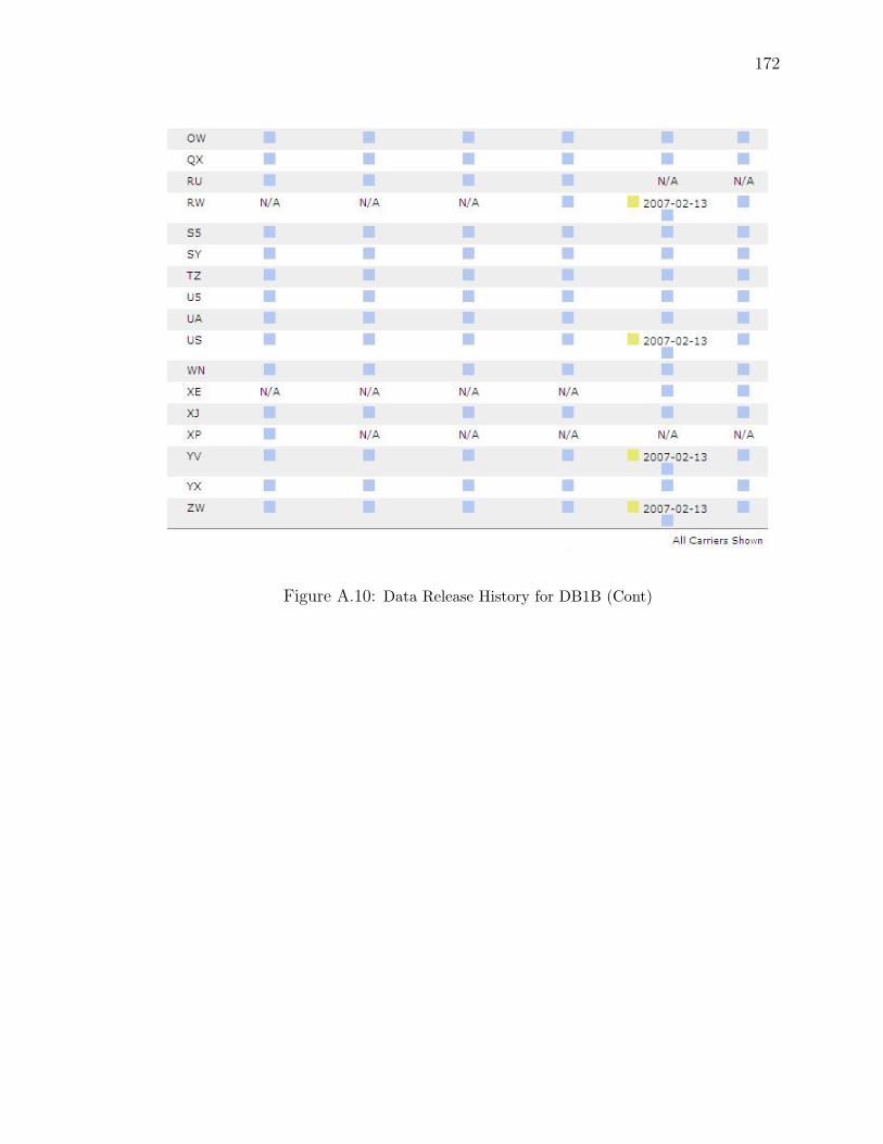
172
Figure A.10: Data Release History for DB1B (Cont)

173
Figure A.11: Database Description and Definitions for DB1B

174
Figure A.12: Field Names and Descriptions for DB1B

175
Appendix B: OEP 35 Airports

176
Figure B.1: Operational Evolution Plan (OEP) 35 Airports

177
Appendix C: SQL Codes For Estimating Passenger
Trip Delay
-- CREATE AOTP* TABLE
DECLARE @FIXED VARCHAR(30)
DECLARE @YEAR INT
DECLARE @MONTH INT
DECLARE @INFILE VARCHAR (40)
DECLARE @CORRECT VARCHAR (200)
DECLARE @CREATE VARCHAR(500)
DECLARE @INSERT VARCHAR (500)
SET @FIXED = ’On\_Time\_On\_Time\_Performance\_’
SET @YEAR = 2006
SET @MONTH=1
SET @INFILE = @FIXED + CAST(@YEAR AS VARCHAR(4)) + ’\_’ + CAST(@MONTH AS
VARCHAR(2))
SET @CREATE = ’SELECT SEQ=IDENTITY(INT,1,1), YEAR, MONTH, DAYOFMONTH, DAYOFWEEK,
ORIGIN, DEST, ARRDELAY, ARRTIME, CRSARRTIME, DEPDELAY, DEPTIME, CRSDEPTIME,
CARRIER, CANCELLED, CANCELLATIONCODE, FLIGHTDATE, FLIGHTNUM, TAILNUM, NASDELAY,
CARRIERDELAY, LATEAIRCRAFTDELAY, SECURITYDELAY, WEATHERDELAY

178
INTO ONTIME35\_2006 FROM ’+ @INFILE + ’ WHERE 1<>1 ’
EXEC(@CREATE)}
-- INSERT IN DATA OF YEAR 2006
WHILE @MONTH<13
BEGIN
SET @INFILE = @FIXED + CAST(@YEAR AS VARCHAR(4)) + ’\_’ + CAST(@MONTH AS
VARCHAR(2))
SET @INSERT = ’INSERT INTO ONTIME35\_2006 SELECT YEAR, MONTH, DAYOFMONTH,
DAYOFWEEK, ORIGIN, DEST, ARRDELAY, ARRTIME, CRSARRTIME, DEPDELAY, DEPTIME,
CRSDEPTIME,CARRIER, CANCELLED, CANCELLATIONCODE, FLIGHTDATE, FLIGHTNUM,
TAILNUM, NASDELAY, CARRIERDELAY,LATEAIRCRAFTDELAY, SECURITYDELAY, WEATHERDELAY
FROM ’ + @INFILE +
’ WHERE ORIGIN IN (SELECT AIRPORT FROM BENCHMARK35)
AND DEST IN (SELECT AIRPORT FROM BENCHMARK35)
ORDER BY ORIGIN, DEST, CARRIER, MONTH, DAYOFMONTH, DEPTIME ’
EXEC(@INSERT)
SET @MONTH = @MONTH + 1
END
------------------------------------------------------
-- CREATE T-100* TABLE
SELECT YEAR, MONTH, ORIGIN, DEST, CARRIER, SUM(SEATS)/SUM(DEPARTURES\_PERFORMED)

179
AS AVGSEAT, SUM(PASSENGERS)/SUM(DEPARTURES\_PERFORMED) AS AVGPAX,
SUM(SEATS)/SUM(DEPARTURES\_PERFORMED)-SUM(PASSENGERS)/SUM(DEPARTURES\_PERFORMED)
AS AVASEAT
INTO LF\_00
FROM T100\_2000
WHERE PASSENGERS>0 AND REGION=’D’ AND DEPARTURES\_PERFORMED>0
GROUP BY YEAR, MONTH, ORIGIN, DEST, CARRIER
ORDER BY YEAR, MONTH, ORIGIN, DEST, CARRIER
------------------------------------------------------
-- DATA PROCESSING AND JOINING
ALTER TABLE ONTIME35\_2006 ADD ARRDATE DATETIME NULL, DEPDATE DATETIME NULL,
AVGPAX INT NULL, AVASEAT INT NULL, PAXDELAY INT NULL, PAXDELAYEQ VARCHAR(50),
AVASEQ VARCHAR(50)
GO
DELETE FROM ONTIME35\_2006
WHERE (CANCELLED=0 AND (DEPTIME=’NULL’OR ARRTIME=’NULL’))
-- UPDATE AIRLINE INFO
UPDATE ONTIME35\_2006 SET CARRIER2=CARRIER
UPDATE ONTIME35\_2006 SET CARRIER=’AA’ WHERE CARRIER2=’MQ’
UPDATE ONTIME35\_2006 SET CARRIER=’DL’ WHERE CARRIER2=’OH’ OR CARRIER2=’EV’
UPDATE ONTIME35\_2006 SET CARRIER=’CO’ WHERE CARRIER2=’RU’
-- CHANGE SOME VARCHAR(255) COLUMNS INTO INT IN

180
-- FIRST NEED TO TAKE CARE OF CHANGING VARCHAR VALUE ‘‘NULL" INTO REAL NULL
UPDATE ONTIME35\_2006 SET ARRTIME = NULL WHERE ARRTIME=’NULL’
UPDATE ONTIME35\_2006 SET DEPTIME = NULL WHERE DEPTIME=’NULL’
UPDATE ONTIME35\_2006 SET CRSARRTIME = NULL WHERE CRSARRTIME=’NULL’
UPDATE ONTIME35\_2006 SET CRSDEPTIME = NULL WHERE CRSDEPTIME=’NULL’
UPDATE ONTIME35\_2006 SET FLIGHTNUM = NULL WHERE FLIGHTNUM=’NULL’
UPDATE ONTIME35\_2006 SET TAILNUM = NULL WHERE TAILNUM=’NULL’
-- THEN CHANGE TYPE
ALTER TABLE ONTIME35\_2006 ALTER COLUMN ARRTIME INT
GO
ALTER TABLE ONTIME35\_2006 ALTER COLUMN DEPTIME INT
GO
ALTER TABLE ONTIME35\_2006 ALTER COLUMN CRSARRTIME INT
GO
ALTER TABLE ONTIME35\_2006 ALTER COLUMN CRSDEPTIME INT
GO
ALTER TABLE ONTIME35\_2006 ALTER COLUMN ORIGIN VARCHAR(3)
GO
ALTER TABLE ONTIME35\_2006 ALTER COLUMN DEST VARCHAR(3)
GO
ALTER TABLE ONTIME35\_2006 ALTER COLUMN FLIGHTNUM INT
GO
ALTER TABLE ONTIME35\_2006 ALTER COLUMN TAILNUM VARCHAR(10)
GO

181
-- SET VALUE FOR COLUMN ARRDATE, DEPDATE FOR NON-CANCELLED FLIGHT
UPDATE ONTIME35\_2006 SET ARRDATE = DATEADD(MI,ARRTIME\%100,FLIGHTDATE),
DEPDATE = DATEADD(MI,DEPTIME\%100,FLIGHTDATE)
WHERE CANCELLED <>1
UPDATE ONTIME35\_2006
SET ARRDATE = DATEADD(HH,(ARRTIME-ARRTIME\%100)/100,ARRDATE),
DEPDATE = DATEADD(HH,(DEPTIME-DEPTIME\%100)/100,DEPDATE)
WHERE CANCELLED <>1
-- SET VALUE FOR COLUMN ARRDATE FOR CANCELLED FLIGHT
UPDATE ONTIME35\_2006 SET ARRDATE = DATEADD(MI,CRSARRTIME\%100,FLIGHTDATE),
DEPDATE = DATEADD(MI,CRSDEPTIME\%100,FLIGHTDATE)
WHERE CANCELLED = 1
UPDATE ONTIME35\_2006
SET ARRDATE = DATEADD(HH,(CRSARRTIME-CRSARRTIME\%100)/100,ARRDATE),
DEPDATE = DATEADD(HH,(CRSDEPTIME-CRSDEPTIME\%100)/100,DEPDATE)
WHERE CANCELLED = 1
-- SET PRIMARY KEY (SO THAT CODE RUNS MUCH MORE EFFICIENTLY)
ALTER TABLE ONTIME35\_2006
ADD CONSTRAINT PK\_ONTIME35\_2006 PRIMARY KEY (SEQ)
GO

182
-- SET VALUE FOR COLUMN AVASEAT FOR NON-CANCELLED FLIGHT
UPDATE ONTIME35\_2006 SET AVASEAT = (SELECT AVASEAT
FROM LF\_06
WHERE LF\_06.YEAR = ONTIME35\_2006.YEAR
AND LF\_06.MONTH = ONTIME35\_2006.MONTH
AND LF\_06.ORIGIN = ONTIME35\_2006.ORIGIN
AND LF\_06.DEST = ONTIME35\_2006.DEST
AND LF\_06.CARRIER = ONTIME35\_2006.CARRIER2)
WHERE CANCELLED <> 1
-- SOME NULL AVASEAT MIGHT BE CAUSED BY COMPANY AND SUBCOMPANY, SO
UPDATE ONTIME35\_2006 SET AVASEAT = (SELECT AVASEAT FROM LF\_06
WHERE LF\_06.YEAR = ONTIME35\_2006.YEAR
AND LF\_06.MONTH = ONTIME35\_2006.MONTH
AND LF\_06.ORIGIN = ONTIME35\_2006.ORIGIN
AND LF\_06.DEST = ONTIME35\_2006.DEST
AND LF\_06.CARRIER = ONTIME35\_2006.CARRIER)
WHERE CANCELLED <> 1 AND AVASEAT IS NULL
-- SOME CARRIER MIGHT NOT BE INCLUDED IN LF TABLE,
-- THEREFORE THEIR AVASEAT ARE SET TO BE THE AVG FOR ALL CARRIERS
UPDATE ONTIME35\_2006 SET AVASEAT = (SELECT AVG(AVASEAT) FROM LF\_06
WHERE LF\_06.YEAR = ONTIME35\_2006.YEAR

183
AND LF\_06.MONTH = ONTIME35\_2006.MONTH
AND LF\_06.ORIGIN = ONTIME35\_2006.ORIGIN
AND LF\_06.DEST=ONTIME35\_2006.DEST)
WHERE CANCELLED <> 1 AND AVASEAT IS NULL
-- CHECK WHETHER THERE IS NOT AVASEAT WITH NULL VALUE WITH CANCELLED<>1
SELECT * FROM ONTIME35\_2006 WHERE AVASEAT IS NULL AND CANCELLED<>1
-- SET VALUE FOR COLUMN AVASEAT FOR CANCELLED FLIGHT
UPDATE ONTIME35\_2006 SET AVASEAT = 0 WHERE CANCELLED = 1
-- SET VALUE TO 0 FOR BOTH NON-CANCELLED AND CANCELLED FLIGHT
UPDATE ONTIME35\_2006 SET PAXDELAY = 0
-- SET VALUE FOR COLUMN AVGPAX
-- GET THE PAX INFO FROM LOADING FACT TABLE
UPDATE ONTIME35\_2006 SET AVGPAX = (SELECT AVGPAX FROM LF\_06
WHERE LF\_06.YEAR = ONTIME35\_2006.YEAR
AND LF\_06.MONTH = ONTIME35\_2006.MONTH
AND LF\_06.ORIGIN = ONTIME35\_2006.ORIGIN
AND LF\_06.DEST = ONTIME35\_2006.DEST
AND LF\_06.CARRIER=ONTIME35\_2006.CARRIER2)
-- FOR THOSE WITH NULL AVGPAX, THEY MIGHT CAUSED BY COMPANY AND SUBCOMPANY

184
UPDATE ONTIME35\_2006 SET AVGPAX = (SELECT AVGPAX FROM LF\_06
WHERE LF\_06.YEAR = ONTIME35\_2006.YEAR
AND LF\_06.MONTH = ONTIME35\_2006.MONTH
AND LF\_06.ORIGIN = ONTIME35\_2006.ORIGIN
AND LF\_06.DEST = ONTIME35\_2006.DEST
AND LF\_06.CARRIER=ONTIME35\_2006.CARRIER)
WHERE AVGPAX IS NULL
-- FOR CARRIER NOT INCLUDED IN LF TABLE, WE USE AVG VALUE OF ALL CARRIERS
UPDATE ONTIME35\_2006 SET AVGPAX = (SELECT AVG(AVGPAX) FROM LF\_06
WHERE LF\_06.YEAR = ONTIME35\_2006.YEAR
AND LF\_06.MONTH = ONTIME35\_2006.MONTH
AND LF\_06.ORIGIN = ONTIME35\_2006.ORIGIN
AND LF\_06.DEST = ONTIME35\_2006.DEST)
WHERE ONTIME35\_2006.AVGPAX IS NULL
-- CHECK WHETHER EVERY RECORD HAS AVGPAX VALUE
SELECT * FROM ONTIME35\_2006 WHERE AVGPAX IS NULL
------------------------------------------------------
-- ESTIMATE PASSENGER TRIP DELAY
-- DECLARE ALL FETCH VARs (START WITH @)
DECLARE @SEQ INT, @YEAR INT, @MONTH INT, @DAYOFMONTH INT, @CANCELLED INT
DECLARE @PAXDELAY INT, @CANCELPAX INT, @AVGPAX INT, @SINGLEPAXDELAY INT

185
DECLARE @NEWSEQ INT, @NEWAVASEAT INT, @NEWDAYOFMONTH INT, @MINSEQ INT
@MAXSEQ INT, @CRSDEPTIME INT
DECLARE @NEWARRDATE DATETIME, @ARRDATE DATETIME, @DEPDATE DATETIME,
@TEMPDATE DATETIME
DECLARE @CARRIER VARCHAR(5), @ORIGIN VARCHAR(5), @DEST VARCHAR(5),
@AVASEQ VARCHAR(50), @PAXDELAYEQ VARCHAR(50)
-- DEFINE A CURSOR FOR LOOP
DECLARE CUR\_CANC\_FLIGHT CURSOR FAST\_FORWARD FOR
SELECT SEQ, YEAR, MONTH, DAYOFMONTH, ORIGIN, DEST, CARRIER, CRSDEPTIME,
CANCELLED, PAXDELAY, ARRDATE, DEPDATE, AVGPAX
FROM ONTIME35\_2006
WHERE CANCELLED = 1 AND SEQ<=(SELECT MAX(SEQ) FROM ONTIME35\_2006)
ORDER BY SEQ
OPEN CUR\_CANC\_FLIGHT
-- READ EACH COLUMN VALUE OF THIS CANCELLED FLIGHT AND GIVE THEIR VALUES
-- TO THOSE CORRESPONDING PARAMETERS
-- @ + COLUMN NAME IS FOR CANCELLED FLIGHTS
-- @ + NEW + COLUMN NAME IS FOR AVAILABLE FLIGHTS
-- NOTE: ‘‘AVG" ARE FOR LF TABLE, AVASEAT IS IN MAIN TABLE,
-- @CANCELPAX IS NOT A COLUMN IN ANY TABLE

186
FETCH NEXT FROM CUR\_CANC\_FLIGHT INTO @SEQ, @YEAR, @MONTH, @DAYOFMONTH,
@ORIGIN, @DEST, @CARRIER, @CRSDEPTIME, @CANCELLED, @PAXDELAY, @ARRDATE,
@DEPDATE,@AVGPAX
WHILE (@@FETCH\_STATUS = 0)
BEGIN
-- INITIALIZATION
SET @PAXDELAY = 0
-- GET THE PAX INFO FROM LOADING FACT TABLE
SELECT @CANCELPAX= @AVGPAX
-- INITIAL @AVASEQ, @PAXDELAYEQ
SET @PAXDELAYEQ = ’ ’
SET @AVASEQ=’ ’
SET @NEWSEQ=’ ’
-- GET MIN MAX NUM FOR ALL FLIGHTS IN O-D/CARRIER COMBINATION
SET @MINSEQ = (SELECT MINSEQ FROM RANGE00
WHERE ORIGIN=@ORIGIN AND DEST=@DEST AND CARRIER=@CARRIER
AND MONTH=@MONTH AND DAYOFMONTH=@DAYOFMONTH)
SET @MAXSEQ = (SELECT MAXSEQ FROM RANGE00
WHERE ORIGIN=@ORIGIN AND DEST=@DEST AND CARRIER=@CARRIER
AND MONTH=@MONTH AND DAYOFMONTH=@DAYOFMONTH+1)

187
WHILE (@CANCELPAX > 0)
BEGIN
-- GET THE NEAREST AVAILABLE FLIGHT INFO - SEQ, ARRDATE AND AVGSEAT
SELECT @NEWSEQ = (SELECT MIN(SEQ) FROM ONTIME35\_2006
WHERE SEQ>=@MINSEQ AND SEQ<=@MAXSEQ AND DEPDATE>@DEPDATE AND
ORIGIN=@ORIGIN AND DEST=@DEST AND CARRIER=@CARRIER
AND CANCELLED=0 AND AVASEAT>0)
IF @NEWSEQ IS NULL
BEGIN
SET @PAXDELAY=900*@AVGPAX
SET @CANCELPAX=0
END
ELSE -- NOW GENERAL CALCULATION BEGINS
BEGIN
SET @NEWARRDATE = (SELECT ARRDATE FROM ONTIME35\_2006 WHERE SEQ=@NEWSEQ)
SET @NEWAVASEAT= (SELECT AVASEAT FROM ONTIME35\_2006 WHERE SEQ = @NEWSEQ)
SET @SINGLEPAXDELAY = DATEDIFF(MI,@ARRDATE, @NEWARRDATE)
IF @SINGLEPAXDELAY < 0 -- IF ACTUAL ARRTIME IS THE NEXT EARLY MORNING
SET @SINGLEPAXDELAY = DATEDIFF(MI,@ARRDATE, @NEWARRDATE) + 1440

188
-- CALCULATE PAXDELAY
IF @CANCELPAX > @NEWAVASEAT -- NO MORE AVAILABLE SEAT
BEGIN
IF @SINGLEPAXDELAY<=900
BEGIN
SET @PAXDELAY = @PAXDELAY + @NEWAVASEAT * @SINGLEPAXDELAY
-- UPDATE \# OF PAX LEFT FOR RELOCATION
SET @CANCELPAX = @CANCELPAX - @NEWAVASEAT
SET @PAXDELAYEQ = @PAXDELAYEQ + CAST(@SINGLEPAXDELAY AS VARCHAR(4))
+ ’X’+ CAST(@NEWAVASEAT AS VARCHAR(3)) + ’,’
SET @AVASEQ = @AVASEQ + CAST(@NEWSEQ AS VARCHAR(10)) + ’,’
END
ELSE -- THAT IS OUT OF UPPER BOUND, PAXDELAY=15 HOURS
BEGIN
SET @SINGLEPAXDELAY = 900
SET @PAXDELAY = @PAXDELAY + @CANCELPAX * 900
SET @PAXDELAYEQ = @PAXDELAYEQ + CAST(@SINGLEPAXDELAY AS VARCHAR(4))
+ ’X’+ CAST(@CANCELPAX AS VARCHAR(3)) + ’,’
SET @CANCELPAX = 0
SET @AVASEQ = @AVASEQ + CAST(@NEWSEQ AS VARCHAR(10))
END

189
-- UPDATE AVASEAT FOR AVAFLIGHT
UPDATE ONTIME35\_2006 SET AVASEAT = 0 WHERE SEQ = @NEWSEQ
END
ELSE -- THERE ARE MORE SEATS THAN RELOCATED PAX
BEGIN
IF @SINGLEPAXDELAY<=900
SET @PAXDELAY = @PAXDELAY + @CANCELPAX * @SINGLEPAXDELAY
ELSE -- THAT IS OUT OF UPPER BOUND OR HAS NEGATIVE PAXDELAY
BEGIN
SET @SINGLEPAXDELAY = 900
SET @PAXDELAY = @PAXDELAY + @CANCELPAX * 900
END
-- UPDATE AVASEAT
UPDATE ONTIME35\_2006
SET AVASEAT = @NEWAVASEAT - @CANCELPAX WHERE SEQ = @NEWSEQ
SET @AVASEQ = @AVASEQ + CAST(@NEWSEQ AS VARCHAR(10))
SET @PAXDELAYEQ = @PAXDELAYEQ + CAST(@SINGLEPAXDELAY AS VARCHAR(4))
+ ’X’+ CAST(@CANCELPAX AS VARCHAR(3))
SET @CANCELPAX = 0

190
END
END
END
-- UPDATE FOR @PAXDELAY
UPDATE ONTIME35\_2006
SET PAXDELAY = @PAXDELAY, AVASEQ = @AVASEQ, PAXDELAYEQ=@PAXDELAYEQ
WHERE SEQ = @SEQ
FETCH NEXT FROM CUR\_CANC\_FLIGHT INTO @SEQ, @YEAR, @MONTH, @DAYOFMONTH,
@ORIGIN, @DEST, @CARRIER, @CRSDEPTIME, @CANCELLED, @PAXDELAY, @ARRDATE,
@DEPDATE, @AVGPAX
END
CLOSE CUR\_CANC\_FLIGHT
DEALLOCATE CUR\_CANC\_FLIGHT
-- DOUBLE CHECK
SELECT * FROM ONTIME35\_2006 WHERE CANCELLED=1}

191
Appendix D: Declarations in PFS
globref outfile = TextIO.stdOut;
val rp=85;
val rs=95;
val rmct=100;
val mctgap=15;
val delaygap=15;
val idenindex=0;
colset Origin = string;
colset Dest = string;
colset Pax = int;
colset Size = int;
colset SchDep = int;
colset SchArr = int;
colset IndexofCarrier = int;
colset FlightIndex = int;
colset TimeStamp = int;
colset PaxGroup= product Origin*Dest*Pax*Size*SchDep
*SchArr*IndexofCarrier*FlightIndex*TimeStamp*Pax timed;
colset Plist = list PaxGroup;

192
colset Q = product IndexofCarrier*Dest;
colset CaPList = product Q*PList;
var r,r’,o’,o0,o00,o01,o2 : Origin;
var d,d’,d0,d00,d01,d1,d2,d3: Dest;
var p,p’,p0,p00,p01, p02,p03,p1,p2,p: Pax;
var s0,s’,s00,s01,s02,s03,s,s1,s2,s3: Size;
var sd,sd’,sd0,sd00,sd01,sd02,sd03,sd1,sd2,sd3:SchDep;
var sa,sa’,sa0,sa00,sa01,sa02,sa03,sa1,sa2,sa3: SchArr;
var i,i’,i0,i00,i01,i02,i03,i1,i2,i3:IndexofCarrier;
var f,f’,f0,f00,f01,f02,f03,f1,f2,f3:FlightIndex;
var ts,t,ts’,ts0,ts00,ts01,ts02,ts03,ts1,ts2,ts3: TimeStamp;
var list1,list2:PList;
fun max(x:int,y:int)=
if x>y then x
else if x=y then x+1
else y;
fun Mtime() =IntInf.toInt (time());
fun lognormal(x:real, y:real)=
let
val m=Math.ln(x)-0.5*Math.ln((y*y)/(x*x)+1.0);

193
val s=Math.sqrt(Math.ln((y*y)/(x*x)+1.0));
in
floor(Math.exp(normal(m,s)))
end;
fun taxiout(r)=
case (r) of
("ATL")=>lognormal(21.8 ,12.9 )|
("BOS")=>lognormal(20.5 ,14.0 )|
("BWI")=>lognormal(14.6 ,11.3 )|
("CLE")=>lognormal(17.3 ,12.2 )|
("CLT")=>lognormal(18.8 ,15.7 )|
("CVG")=>lognormal(16.5 ,9.1 )|
("DCA")=>lognormal(18.8 ,17.8 )|
("DEN")=>lognormal(15.0 ,8.9 )|
("DFW")=>lognormal(20.2 ,18.3 )|
("DTW")=>lognormal(19.2 ,14.0 )|
("EWR")=>lognormal(30.6 ,23.7 )|
("FLL")=>lognormal(17.3 ,10.9 )|
("IAD")=>lognormal(22.7 ,18.5 )|
("IAH")=>lognormal(24.9 ,18.0 )|
("JFK")=>lognormal(35.1 ,22.8 )|
("LAS")=>lognormal(17.4 ,8.6 )|
("LAX")=>lognormal(15.9 ,8.0 )|

194
("LGA")=>lognormal(27.3 ,21.9 )|
("MCO")=>lognormal(14.3 ,9.1 )|
("MDW")=>lognormal(16.0 ,15.1 )|
("MEM")=>lognormal(16.2 ,9.7 )|
("MIA")=>lognormal(18.7 ,14.7 )|
("MSP")=>lognormal(20.5 ,11.8 )|
("ORD")=>lognormal(24.3 ,23.0 )|
("PDX")=>lognormal(12.1 ,5.0 )|
("PHL")=>lognormal(30.5 ,25.2 )|
("PHX")=>lognormal(15.8 ,8.6 )|
("PIT")=>lognormal(14.5 ,11.5 )|
("SAN")=>lognormal(15.5 ,10.3 )|
("SEA")=>lognormal(14.5 ,5.9 )|
("SFO")=>lognormal(17.1 ,8.1 )|
("SLC")=>lognormal(17.6 ,7.3 )|
("STL")=>lognormal(13.3 ,8.0 )|
("TPA")=>lognormal(13.8 ,10.2 )|
_=>0;
fun airtime(r,d)=
case (r,d) of
("ATL","BOS")=>lognormal(123.6 ,6.9 )|
("ATL","BWI")=>lognormal(81.5 ,5.8 )|
("ATL","CLE")=>lognormal(75.3 ,80.5 )|

195
("ATL","CLT")=>lognormal(43.5 ,5.5 )|
("ATL","CVG")=>lognormal(59.2 ,5.8 )|
("ATL","DCA")=>lognormal(78.3 ,5.6 )|
("ATL","DEN")=>lognormal(157.1 ,7.5 )|
("ATL","DFW")=>lognormal(103.7 ,6.5 )|
("ATL","DTW")=>lognormal(87.1 ,6.8 )|
("ATL","EWR")=>lognormal(107.7 ,11.6 )|
("ATL","FLL")=>lognormal(84.0 ,6.6 )|
("ATL","IAD")=>lognormal(79.0 ,6.3 )|
("ATL","IAH")=>lognormal(98.3 ,8.8 )|
("ATL","JFK")=>lognormal(108.0 ,8.8 )|
("ATL","LAS")=>lognormal(218.0 ,7.8 )|
("ATL","LAX")=>lognormal(236.5 ,8.5 )|
("ATL","LGA")=>lognormal(106.8 ,9.4 )|
("ATL","MCO")=>lognormal(62.1 ,7.5 )|
("ATL","MDW")=>lognormal(83.7 ,8.2 )|
("ATL","MEM")=>lognormal(52.5 ,8.4 )|
("ATL","MIA")=>lognormal(85.1 ,6.7 )|
("ATL","MSP")=>lognormal(127.8 ,9.6 )|
("ATL","ORD")=>lognormal(91.5 ,12.2 )|
("ATL","PDX")=>lognormal(272.6 ,7.1 )|
("ATL","PHL")=>lognormal(96.2 ,7.6 )|
("ATL","PHX")=>lognormal(204.6 ,7.9 )|
("ATL","PIT")=>lognormal(42.3 ,206.9 )|

196
("ATL","SAN")=>lognormal(231.7 ,7.1 )|
("ATL","SEA")=>lognormal(277.3 ,8.4 )|
("ATL","SFO")=>lognormal(264.7 ,9.2 )|
("ATL","SLC")=>lognormal(202.9 ,7.7 )|
("ATL","STL")=>lognormal(73.0 ,6.5 )|
("ATL","TPA")=>lognormal(60.9 ,5.5 )|
("BOS","ATL")=>lognormal(137.0 ,11.2 )|
("BOS","BWI")=>lognormal(63.0 ,5.3 )|
("BOS","CLE")=>lognormal(90.5 ,4.9 )|
("BOS","CLT")=>lognormal(108.4 ,12.6 )|
("BOS","CVG")=>lognormal(113.4 ,7.3 )|
("BOS","DCA")=>lognormal(70.5 ,7.6 )|
("BOS","DEN")=>lognormal(213.3 ,47.8 )|
("BOS","DFW")=>lognormal(209.1 ,9.5 )|
("BOS","DTW")=>lognormal(97.4 ,8.1 )|
("BOS","EWR")=>lognormal(51.5 ,8.2 )|
("BOS","FLL")=>lognormal(164.5 ,7.9 )|
("BOS","IAD")=>lognormal(73.5 ,8.4 )|
("BOS","IAH")=>lognormal(217.9 ,11.7 )|
("BOS","JFK")=>lognormal(44.2 ,7.6 )|
("BOS","LAS")=>lognormal(269.6 ,72.1 )|
("BOS","LAX")=>lognormal(330.1 ,13.0 )|
("BOS","LGA")=>lognormal(43.6 ,6.9 )|
("BOS","MCO")=>lognormal(151.5 ,8.8 )|

197
("BOS","MDW")=>lognormal(128.2 ,7.8 )|
("BOS","MIA")=>lognormal(166.3 ,9.2 )|
("BOS","MSP")=>lognormal(161.0 ,10.0 )|
("BOS","ORD")=>lognormal(129.6 ,9.7 )|
("BOS","PHL")=>lognormal(60.3 ,7.4 )|
("BOS","PHX")=>lognormal(295.1 ,14.7 )|
("BOS","PIT")=>lognormal(77.1 ,6.1 )|
("BOS","SAN")=>lognormal(327.5 ,10.0 )|
("BOS","SEA")=>lognormal(333.0 ,12.4 )|
("BOS","SFO")=>lognormal(345.3 ,13.0 )|
("BOS","SLC")=>lognormal(279.7 ,11.1 )|
("BOS","STL")=>lognormal(150.2 ,7.3 )|
("BOS","TPA")=>lognormal(162.1 ,8.4 )|
("BWI","ATL")=>lognormal(86.0 ,61.7 )|
("BWI","BOS")=>lognormal(60.5 ,5.5 )|
("BWI","CLE")=>lognormal(53.2 ,5.0 )|
("BWI","CLT")=>lognormal(59.3 ,8.8 )|
("BWI","CVG")=>lognormal(71.9 ,5.6 )|
("BWI","DEN")=>lognormal(198.8 ,9.9 )|
("BWI","DFW")=>lognormal(162.0 ,9.9 )|
("BWI","DTW")=>lognormal(65.8 ,5.0 )|
("BWI","EWR")=>lognormal(39.4 ,7.2 )|
("BWI","FLL")=>lognormal(129.8 ,8.5 )|
("BWI","IAH")=>lognormal(168.5 ,9.9 )|

198
("BWI","JFK")=>lognormal(43.4 ,6.5 )|
("BWI","LAS")=>lognormal(269.5 ,11.7 )|
("BWI","LAX")=>lognormal(292.5 ,11.4 )|
("BWI","MCO")=>lognormal(108.6 ,5.9 )|
("BWI","MDW")=>lognormal(94.6 ,7.0 )|
("BWI","MEM")=>lognormal(112.5 ,4.4 )|
("BWI","MIA")=>lognormal(125.9 ,7.2 )|
("BWI","MSP")=>lognormal(133.3 ,8.9 )|
("BWI","ORD")=>lognormal(97.1 ,9.4 )|
("BWI","PHL")=>lognormal(28.2 ,4.9 )|
("BWI","PHX")=>lognormal(256.7 ,11.9 )|
("BWI","PIT")=>lognormal(37.5 ,6.0 )|
("BWI","SAN")=>lognormal(289.2 ,12.7 )|
("BWI","SFO")=>lognormal(308.9 ,11.2 )|
("BWI","SLC")=>lognormal(250.2 ,8.8 )|
("BWI","STL")=>lognormal(107.5 ,4.9 )|
("BWI","TPA")=>lognormal(118.2 ,8.5 )|
("CLE","ATL")=>lognormal(75.2 ,133.8 )|
("CLE","BOS")=>lognormal(81.2 ,8.3 )|
("CLE","BWI")=>lognormal(55.6 ,5.1 )|
("CLE","CLT")=>lognormal(69.1 ,5.8 )|
("CLE","CVG")=>lognormal(44.4 ,4.9 )|
("CLE","DCA")=>lognormal(54.0 ,8.8 )|
("CLE","DEN")=>lognormal(160.3 ,8.8 )|

199
("CLE","DFW")=>lognormal(140.3 ,10.8 )|
("CLE","DTW")=>lognormal(26.6 ,3.9 )|
("CLE","EWR")=>lognormal(66.5 ,7.9 )|
("CLE","FLL")=>lognormal(147.7 ,6.5 )|
("CLE","IAD")=>lognormal(52.8 ,5.3 )|
("CLE","IAH")=>lognormal(148.8 ,10.2 )|
("CLE","JFK")=>lognormal(74.5 ,7.1 )|
("CLE","LAS")=>lognormal(230.7 ,10.6 )|
("CLE","LAX")=>lognormal(255.0 ,9.9 )|
("CLE","LGA")=>lognormal(69.6 ,7.0 )|
("CLE","MCO")=>lognormal(120.9 ,5.1 )|
("CLE","MDW")=>lognormal(52.7 ,4.9 )|
("CLE","MEM")=>lognormal(91.4 ,3.7 )|
("CLE","MIA")=>lognormal(150.6 ,7.3 )|
("CLE","MSP")=>lognormal(97.6 ,8.5 )|
("CLE","ORD")=>lognormal(55.4 ,5.4 )|
("CLE","PHL")=>lognormal(61.7 ,7.0 )|
("CLE","PHX")=>lognormal(222.7 ,10.3 )|
("CLE","SAN")=>lognormal(250.9 ,8.0 )|
("CLE","SEA")=>lognormal(264.8 ,11.6 )|
("CLE","SFO")=>lognormal(272.6 ,10.3 )|
("CLE","STL")=>lognormal(75.4 ,4.5 )|
("CLE","TPA")=>lognormal(129.6 ,6.9 )|
("CLT","ATL")=>lognormal(46.1 ,8.2 )|

200
("CLT","BOS")=>lognormal(100.6 ,6.6 )|
("CLT","BWI")=>lognormal(57.8 ,6.4 )|
("CLT","CLE")=>lognormal(68.4 ,6.6 )|
("CLT","CVG")=>lognormal(55.1 ,96.2 )|
("CLT","DCA")=>lognormal(54.6 ,5.2 )|
("CLT","DEN")=>lognormal(178.7 ,8.5 )|
("CLT","DFW")=>lognormal(129.3 ,7.5 )|
("CLT","DTW")=>lognormal(80.2 ,6.6 )|
("CLT","EWR")=>lognormal(84.2 ,10.0 )|
("CLT","FLL")=>lognormal(90.7 ,6.3 )|
("CLT","IAD")=>lognormal(58.9 ,6.9 )|
("CLT","IAH")=>lognormal(130.1 ,7.3 )|
("CLT","JFK")=>lognormal(88.2 ,12.3 )|
("CLT","LAS")=>lognormal(239.7 ,8.3 )|
("CLT","LAX")=>lognormal(263.0 ,9.3 )|
("CLT","LGA")=>lognormal(82.8 ,9.3 )|
("CLT","MCO")=>lognormal(66.4 ,6.6 )|
("CLT","MEM")=>lognormal(74.5 ,3.2 )|
("CLT","MIA")=>lognormal(93.0 ,5.9 )|
("CLT","MSP")=>lognormal(137.4 ,8.6 )|
("CLT","ORD")=>lognormal(93.9 ,12.5 )|
("CLT","PHL")=>lognormal(71.8 ,6.8 )|
("CLT","PHX")=>lognormal(228.1 ,8.4 )|
("CLT","PIT")=>lognormal(57.7 ,5.6 )|

201
("CLT","SAN")=>lognormal(258.6 ,10.5 )|
("CLT","SEA")=>lognormal(299.8 ,7.4 )|
("CLT","SFO")=>lognormal(288.4 ,9.8 )|
("CLT","STL")=>lognormal(88.0 ,3.8 )|
("CLT","TPA")=>lognormal(72.7 ,7.9 )|
("CVG","ATL")=>lognormal(69.3 ,8.5 )|
("CVG","BOS")=>lognormal(104.4 ,8.6 )|
("CVG","BWI")=>lognormal(65.6 ,6.9 )|
("CVG","CLE")=>lognormal(40.4 ,3.7 )|
("CVG","CLT")=>lognormal(57.2 ,8.5 )|
("CVG","DCA")=>lognormal(63.5 ,7.2 )|
("CVG","DEN")=>lognormal(142.1 ,8.2 )|
("CVG","DFW")=>lognormal(115.2 ,8.9 )|
("CVG","DTW")=>lognormal(44.3 ,6.5 )|
("CVG","EWR")=>lognormal(92.1 ,9.4 )|
("CVG","FLL")=>lognormal(134.2 ,7.6 )|
("CVG","IAD")=>lognormal(63.3 ,6.0 )|
("CVG","IAH")=>lognormal(127.3 ,11.9 )|
("CVG","JFK")=>lognormal(95.0 ,9.2 )|
("CVG","LAS")=>lognormal(213.9 ,9.6 )|
("CVG","LAX")=>lognormal(234.9 ,9.2 )|
("CVG","LGA")=>lognormal(90.4 ,8.6 )|
("CVG","MCO")=>lognormal(103.9 ,6.4 )|
("CVG","MEM")=>lognormal(62.1 ,5.2 )|

202
("CVG","MIA")=>lognormal(132.0 ,13.8 )|
("CVG","MSP")=>lognormal(94.4 ,9.5 )|
("CVG","ORD")=>lognormal(49.3 ,10.7 )|
("CVG","PDX")=>lognormal(254.2 ,7.9 )|
("CVG","PHL")=>lognormal(76.9 ,8.6 )|
("CVG","PHX")=>lognormal(202.3 ,7.9 )|
("CVG","PIT")=>lognormal(26.0 ,161.7 )|
("CVG","SAN")=>lognormal(233.4 ,8.8 )|
("CVG","SEA")=>lognormal(259.3 ,8.6 )|
("CVG","SFO")=>lognormal(253.8 ,9.2 )|
("CVG","SLC")=>lognormal(192.3 ,7.6 )|
("CVG","STL")=>lognormal(56.5 ,6.5 )|
("CVG","TPA")=>lognormal(106.9 ,6.3 )|
("DCA","ATL")=>lognormal(85.0 ,10.0 )|
("DCA","BOS")=>lognormal(63.9 ,6.8 )|
("DCA","CLE")=>lognormal(55.6 ,7.4 )|
("DCA","CLT")=>lognormal(55.9 ,8.6 )|
("DCA","CVG")=>lognormal(67.3 ,5.2 )|
("DCA","DEN")=>lognormal(201.0 ,11.0 )|
("DCA","DFW")=>lognormal(160.1 ,7.5 )|
("DCA","DTW")=>lognormal(67.3 ,7.1 )|
("DCA","EWR")=>lognormal(43.9 ,5.7 )|
("DCA","FLL")=>lognormal(125.7 ,6.9 )|
("DCA","IAH")=>lognormal(163.3 ,8.6 )|

203
("DCA","JFK")=>lognormal(46.1 ,6.8 )|
("DCA","LAS")=>lognormal(266.4 ,12.4 )|
("DCA","LAX")=>lognormal(288.9 ,12.9 )|
("DCA","LGA")=>lognormal(44.2 ,6.3 )|
("DCA","MCO")=>lognormal(109.6 ,5.7 )|
("DCA","MDW")=>lognormal(90.6 ,6.2 )|
("DCA","MEM")=>lognormal(107.0 ,6.0 )|
("DCA","MIA")=>lognormal(125.0 ,6.8 )|
("DCA","MSP")=>lognormal(132.7 ,8.6 )|
("DCA","ORD")=>lognormal(94.4 ,10.0 )|
("DCA","PHL")=>lognormal(30.8 ,4.3 )|
("DCA","PHX")=>lognormal(253.8 ,11.1 )|
("DCA","PIT")=>lognormal(37.2 ,5.7 )|
("DCA","SEA")=>lognormal(311.9 ,11.5 )|
("DCA","SLC")=>lognormal(247.2 ,9.0 )|
("DCA","STL")=>lognormal(104.7 ,4.4 )|
("DCA","TPA")=>lognormal(116.2 ,8.1 )|
("DEN","ATL")=>lognormal(154.6 ,12.1 )|
("DEN","BOS")=>lognormal(225.1 ,41.4 )|
("DEN","BWI")=>lognormal(183.2 ,11.0 )|
("DEN","CLE")=>lognormal(148.5 ,8.7 )|
("DEN","CLT")=>lognormal(166.0 ,9.0 )|
("DEN","CVG")=>lognormal(135.9 ,9.0 )|
("DEN","DCA")=>lognormal(182.6 ,11.9 )|

204
("DEN","DFW")=>lognormal(87.5 ,5.3 )|
("DEN","DTW")=>lognormal(142.1 ,8.2 )|
("DEN","EWR")=>lognormal(202.0 ,13.8 )|
("DEN","FLL")=>lognormal(213.2 ,8.7 )|
("DEN","IAD")=>lognormal(176.9 ,9.2 )|
("DEN","IAH")=>lognormal(117.8 ,8.2 )|
("DEN","JFK")=>lognormal(322.5 ,13.6 )|
("DEN","LAS")=>lognormal(87.1 ,4.1 )|
("DEN","LAX")=>lognormal(113.6 ,4.9 )|
("DEN","LGA")=>lognormal(200.7 ,12.9 )|
("DEN","MCO")=>lognormal(191.9 ,7.3 )|
("DEN","MDW")=>lognormal(115.7 ,6.9 )|
("DEN","MEM")=>lognormal(114.5 ,7.2 )|
("DEN","MIA")=>lognormal(210.9 ,8.1 )|
("DEN","MSP")=>lognormal(93.2 ,6.7 )|
("DEN","ORD")=>lognormal(116.6 ,7.3 )|
("DEN","PDX")=>lognormal(137.7 ,5.2 )|
("DEN","PHL")=>lognormal(194.6 ,12.2 )|
("DEN","PHX")=>lognormal(86.1 ,4.7 )|
("DEN","PIT")=>lognormal(158.2 ,6.5 )|
("DEN","SAN")=>lognormal(113.6 ,5.5 )|
("DEN","SEA")=>lognormal(144.2 ,6.1 )|
("DEN","SFO")=>lognormal(127.6 ,6.4 )|
("DEN","SLC")=>lognormal(63.3 ,4.4 )|

205
("DEN","STL")=>lognormal(100.9 ,4.7 )|
("DEN","TPA")=>lognormal(186.1 ,7.0 )|
("DFW","ATL")=>lognormal(105.2 ,10.2 )|
("DFW","BOS")=>lognormal(194.1 ,9.5 )|
("DFW","BWI")=>lognormal(153.7 ,9.1 )|
("DFW","CLE")=>lognormal(130.0 ,8.2 )|
("DFW","CLT")=>lognormal(125.2 ,6.1 )|
("DFW","CVG")=>lognormal(110.4 ,5.0 )|
("DFW","DCA")=>lognormal(150.9 ,7.9 )|
("DFW","DEN")=>lognormal(92.6 ,7.0 )|
("DFW","DTW")=>lognormal(131.2 ,9.1 )|
("DFW","EWR")=>lognormal(182.5 ,14.7 )|
("DFW","FLL")=>lognormal(147.1 ,9.3 )|
("DFW","IAD")=>lognormal(149.4 ,8.1 )|
("DFW","IAH")=>lognormal(42.9 ,5.3 )|
("DFW","JFK")=>lognormal(183.3 ,11.5 )|
("DFW","LAS")=>lognormal(138.4 ,5.6 )|
("DFW","LAX")=>lognormal(156.4 ,5.6 )|
("DFW","LGA")=>lognormal(182.9 ,12.0 )|
("DFW","MCO")=>lognormal(131.3 ,8.3 )|
("DFW","MDW")=>lognormal(108.6 ,12.0 )|
("DFW","MEM")=>lognormal(65.1 ,5.0 )|
("DFW","MIA")=>lognormal(142.6 ,6.6 )|
("DFW","MSP")=>lognormal(118.6 ,7.8 )|

206
("DFW","ORD")=>lognormal(110.1 ,8.8 )|
("DFW","PDX")=>lognormal(208.7 ,5.5 )|
("DFW","PHL")=>lognormal(170.8 ,10.9 )|
("DFW","PHX")=>lognormal(119.9 ,6.2 )|
("DFW","PIT")=>lognormal(135.3 ,5.5 )|
("DFW","SAN")=>lognormal(149.5 ,6.7 )|
("DFW","SEA")=>lognormal(216.4 ,7.0 )|
("DFW","SFO")=>lognormal(188.9 ,6.7 )|
("DFW","SLC")=>lognormal(133.3 ,5.3 )|
("DFW","STL")=>lognormal(78.3 ,4.7 )|
("DFW","TPA")=>lognormal(124.4 ,7.2 )|
("DTW","ATL")=>lognormal(91.8 ,9.3 )|
("DTW","BOS")=>lognormal(86.7 ,6.4 )|
("DTW","BWI")=>lognormal(66.6 ,5.6 )|
("DTW","CLE")=>lognormal(24.7 ,4.4 )|
("DTW","CLT")=>lognormal(77.1 ,6.1 )|
("DTW","CVG")=>lognormal(47.3 ,5.6 )|
("DTW","DCA")=>lognormal(63.2 ,5.6 )|
("DTW","DEN")=>lognormal(152.6 ,10.0 )|
("DTW","DFW")=>lognormal(136.6 ,9.7 )|
("DTW","EWR")=>lognormal(75.8 ,7.7 )|
("DTW","FLL")=>lognormal(151.8 ,9.0 )|
("DTW","IAD")=>lognormal(65.2 ,5.9 )|
("DTW","IAH")=>lognormal(149.5 ,11.7 )|

207
("DTW","JFK")=>lognormal(77.8 ,7.1 )|
("DTW","LAS")=>lognormal(223.4 ,10.1 )|
("DTW","LAX")=>lognormal(247.7 ,10.7 )|
("DTW","LGA")=>lognormal(76.9 ,7.9 )|
("DTW","MCO")=>lognormal(128.4 ,7.3 )|
("DTW","MDW")=>lognormal(44.6 ,4.4 )|
("DTW","MEM")=>lognormal(88.6 ,4.9 )|
("DTW","MIA")=>lognormal(151.7 ,6.9 )|
("DTW","MSP")=>lognormal(87.2 ,7.4 )|
("DTW","ORD")=>lognormal(45.2 ,5.7 )|
("DTW","PDX")=>lognormal(257.0 ,9.3 )|
("DTW","PHL")=>lognormal(71.8 ,6.6 )|
("DTW","PHX")=>lognormal(215.2 ,10.5 )|
("DTW","PIT")=>lognormal(36.6 ,3.0 )|
("DTW","SAN")=>lognormal(245.9 ,10.5 )|
("DTW","SEA")=>lognormal(258.9 ,9.4 )|
("DTW","SFO")=>lognormal(264.4 ,11.5 )|
("DTW","SLC")=>lognormal(201.7 ,8.8 )|
("DTW","STL")=>lognormal(70.7 ,5.3 )|
("DTW","TPA")=>lognormal(128.9 ,5.1 )|
("EWR","ATL")=>lognormal(109.3 ,10.1 )|
("EWR","BOS")=>lognormal(39.9 ,4.5 )|
("EWR","BWI")=>lognormal(36.3 ,4.4 )|
("EWR","CLE")=>lognormal(65.1 ,7.6 )|

208
("EWR","CLT")=>lognormal(81.1 ,9.6 )|
("EWR","CVG")=>lognormal(90.3 ,5.6 )|
("EWR","DCA")=>lognormal(39.8 ,5.6 )|
("EWR","DEN")=>lognormal(213.3 ,10.1 )|
("EWR","DFW")=>lognormal(184.3 ,9.8 )|
("EWR","DTW")=>lognormal(81.7 ,8.2 )|
("EWR","FLL")=>lognormal(145.5 ,9.9 )|
("EWR","IAD")=>lognormal(45.7 ,6.5 )|
("EWR","IAH")=>lognormal(185.8 ,11.6 )|
("EWR","LAS")=>lognormal(280.5 ,12.3 )|
("EWR","LAX")=>lognormal(305.5 ,11.6 )|
("EWR","MCO")=>lognormal(128.2 ,9.4 )|
("EWR","MDW")=>lognormal(104.6 ,6.8 )|
("EWR","MEM")=>lognormal(135.2 ,7.4 )|
("EWR","MIA")=>lognormal(146.2 ,8.1 )|
("EWR","MSP")=>lognormal(146.7 ,8.8 )|
("EWR","ORD")=>lognormal(110.2 ,7.7 )|
("EWR","PDX")=>lognormal(318.9 ,11.7 )|
("EWR","PHL")=>lognormal(29.7 ,5.1 )|
("EWR","PHX")=>lognormal(271.6 ,11.2 )|
("EWR","PIT")=>lognormal(54.3 ,5.3 )|
("EWR","SAN")=>lognormal(303.1 ,10.6 )|
("EWR","SEA")=>lognormal(318.1 ,12.4 )|
("EWR","SFO")=>lognormal(325.9 ,11.6 )|

209
("EWR","SLC")=>lognormal(262.5 ,11.2 )|
("EWR","STL")=>lognormal(127.6 ,5.7 )|
("EWR","TPA")=>lognormal(139.1 ,11.0 )|
("FLL","ATL")=>lognormal(86.7 ,10.6 )|
("FLL","BOS")=>lognormal(161.2 ,6.4 )|
("FLL","BWI")=>lognormal(126.9 ,7.0 )|
("FLL","CLE")=>lognormal(141.0 ,6.1 )|
("FLL","CLT")=>lognormal(95.4 ,6.3 )|
("FLL","CVG")=>lognormal(125.5 ,6.9 )|
("FLL","DCA")=>lognormal(121.0 ,6.3 )|
("FLL","DEN")=>lognormal(218.1 ,10.1 )|
("FLL","DFW")=>lognormal(150.4 ,8.1 )|
("FLL","DTW")=>lognormal(151.1 ,9.5 )|
("FLL","EWR")=>lognormal(150.7 ,10.3 )|
("FLL","IAD")=>lognormal(119.9 ,4.6 )|
("FLL","IAH")=>lognormal(127.8 ,7.9 )|
("FLL","JFK")=>lognormal(146.1 ,66.1 )|
("FLL","LAS")=>lognormal(268.4 ,11.1 )|
("FLL","LAX")=>lognormal(285.4 ,6.7 )|
("FLL","LGA")=>lognormal(147.2 ,10.7 )|
("FLL","MCO")=>lognormal(35.4 ,3.3 )|
("FLL","MDW")=>lognormal(154.0 ,8.4 )|
("FLL","MEM")=>lognormal(114.6 ,5.9 )|
("FLL","MSP")=>lognormal(195.2 ,7.8 )|

210
("FLL","ORD")=>lognormal(160.5 ,9.0 )|
("FLL","PHL")=>lognormal(139.7 ,9.5 )|
("FLL","PHX")=>lognormal(253.2 ,9.1 )|
("FLL","PIT")=>lognormal(132.2 ,5.8 )|
("FLL","SLC")=>lognormal(264.3 ,7.7 )|
("FLL","STL")=>lognormal(137.9 ,7.0 )|
("FLL","TPA")=>lognormal(38.1 ,3.8 )|
("IAD","ATL")=>lognormal(82.9 ,10.1 )|
("IAD","BOS")=>lognormal(65.6 ,5.7 )|
("IAD","CLE")=>lognormal(52.3 ,6.4 )|
("IAD","CLT")=>lognormal(54.0 ,9.2 )|
("IAD","CVG")=>lognormal(67.3 ,6.3 )|
("IAD","DEN")=>lognormal(192.9 ,11.5 )|
("IAD","DFW")=>lognormal(155.6 ,9.1 )|
("IAD","DTW")=>lognormal(65.5 ,7.4 )|
("IAD","EWR")=>lognormal(46.5 ,6.5 )|
("IAD","FLL")=>lognormal(128.2 ,7.5 )|
("IAD","IAH")=>lognormal(163.0 ,9.2 )|
("IAD","JFK")=>lognormal(49.0 ,7.0 )|
("IAD","LAS")=>lognormal(263.1 ,10.3 )|
("IAD","LAX")=>lognormal(283.5 ,10.4 )|
("IAD","LGA")=>lognormal(46.1 ,7.7 )|
("IAD","MCO")=>lognormal(105.1 ,6.6 )|
("IAD","MDW")=>lognormal(88.9 ,6.4 )|

211
("IAD","MIA")=>lognormal(130.2 ,6.7 )|
("IAD","MSP")=>lognormal(132.8 ,7.6 )|
("IAD","ORD")=>lognormal(92.0 ,12.3 )|
("IAD","PDX")=>lognormal(304.7 ,9.4 )|
("IAD","PHX")=>lognormal(252.5 ,11.4 )|
("IAD","PIT")=>lognormal(33.7 ,5.0 )|
("IAD","SAN")=>lognormal(245.4 ,73.9 )|
("IAD","SEA")=>lognormal(304.3 ,10.1 )|
("IAD","SFO")=>lognormal(304.4 ,11.3 )|
("IAD","SLC")=>lognormal(242.2 ,9.2 )|
("IAD","TPA")=>lognormal(110.9 ,7.0 )|
("IAH","ATL")=>lognormal(101.5 ,9.9 )|
("IAH","BOS")=>lognormal(202.4 ,9.2 )|
("IAH","BWI")=>lognormal(160.6 ,8.1 )|
("IAH","CLE")=>lognormal(136.9 ,7.4 )|
("IAH","CLT")=>lognormal(125.7 ,6.3 )|
("IAH","CVG")=>lognormal(119.0 ,7.5 )|
("IAH","DCA")=>lognormal(158.1 ,8.6 )|
("IAH","DEN")=>lognormal(117.5 ,8.3 )|
("IAH","DFW")=>lognormal(43.3 ,6.1 )|
("IAH","DTW")=>lognormal(140.7 ,12.3 )|
("IAH","EWR")=>lognormal(184.6 ,14.0 )|
("IAH","FLL")=>lognormal(125.9 ,8.2 )|
("IAH","IAD")=>lognormal(160.6 ,8.2 )|

212
("IAH","JFK")=>lognormal(192.3 ,6.3 )|
("IAH","LAS")=>lognormal(156.8 ,5.1 )|
("IAH","LAX")=>lognormal(170.8 ,6.1 )|
("IAH","LGA")=>lognormal(186.4 ,12.6 )|
("IAH","MCO")=>lognormal(115.8 ,5.8 )|
("IAH","MEM")=>lognormal(70.8 ,5.3 )|
("IAH","MIA")=>lognormal(126.6 ,8.6 )|
("IAH","MSP")=>lognormal(139.0 ,7.1 )|
("IAH","ORD")=>lognormal(125.1 ,10.5 )|
("IAH","PDX")=>lognormal(230.7 ,8.4 )|
("IAH","PHL")=>lognormal(173.9 ,9.6 )|
("IAH","PHX")=>lognormal(133.9 ,5.6 )|
("IAH","PIT")=>lognormal(146.3 ,7.5 )|
("IAH","SAN")=>lognormal(162.4 ,6.5 )|
("IAH","SEA")=>lognormal(239.7 ,8.5 )|
("IAH","SFO")=>lognormal(210.5 ,9.4 )|
("IAH","SLC")=>lognormal(160.3 ,6.7 )|
("IAH","STL")=>lognormal(98.3 ,4.6 )|
("IAH","TPA")=>lognormal(106.4 ,7.2 )|
("JFK","ATL")=>lognormal(112.7 ,12.1 )|
("JFK","BOS")=>lognormal(39.1 ,10.0 )|
("JFK","BWI")=>lognormal(36.8 ,6.6 )|
("JFK","CLE")=>lognormal(71.2 ,6.7 )|
("JFK","CLT")=>lognormal(89.9 ,26.0 )|

213
("JFK","CVG")=>lognormal(92.0 ,7.3 )|
("JFK","DCA")=>lognormal(47.6 ,5.0 )|
("JFK","DEN")=>lognormal(94.6 ,11.8 )|
("JFK","DFW")=>lognormal(181.8 ,11.7 )|
("JFK","DTW")=>lognormal(85.3 ,13.6 )|
("JFK","FLL")=>lognormal(143.6 ,8.2 )|
("JFK","IAD")=>lognormal(50.0 ,7.6 )|
("JFK","IAH")=>lognormal(190.5 ,10.5 )|
("JFK","LAS")=>lognormal(185.8 ,89.4 )|
("JFK","LAX")=>lognormal(309.8 ,11.7 )|
("JFK","MCO")=>lognormal(128.4 ,7.6 )|
("JFK","MIA")=>lognormal(142.0 ,7.5 )|
("JFK","MSP")=>lognormal(151.9 ,9.0 )|
("JFK","ORD")=>lognormal(122.4 ,33.7 )|
("JFK","PDX")=>lognormal(144.2 ,11.6 )|
("JFK","PHL")=>lognormal(31.0 ,5.9 )|
("JFK","PHX")=>lognormal(230.5 ,78.4 )|
("JFK","PIT")=>lognormal(64.4 ,10.4 )|
("JFK","SAN")=>lognormal(198.1 ,89.0 )|
("JFK","SEA")=>lognormal(270.7 ,81.5 )|
("JFK","SFO")=>lognormal(329.6 ,13.1 )|
("JFK","SLC")=>lognormal(233.6 ,55.2 )|
("JFK","STL")=>lognormal(127.2 ,8.6 )|
("JFK","TPA")=>lognormal(138.1 ,8.4 )|

214
("LAS","ATL")=>lognormal(214.5 ,11.1 )|
("LAS","BOS")=>lognormal(314.9 ,72.3 )|
("LAS","BWI")=>lognormal(250.1 ,12.5 )|
("LAS","CLE")=>lognormal(214.7 ,8.3 )|
("LAS","CLT")=>lognormal(228.2 ,7.7 )|
("LAS","CVG")=>lognormal(203.5 ,8.7 )|
("LAS","DCA")=>lognormal(248.5 ,8.5 )|
("LAS","DEN")=>lognormal(86.9 ,4.8 )|
("LAS","DFW")=>lognormal(133.5 ,6.1 )|
("LAS","DTW")=>lognormal(212.3 ,9.6 )|
("LAS","EWR")=>lognormal(267.7 ,13.4 )|
("LAS","FLL")=>lognormal(258.5 ,6.8 )|
("LAS","IAD")=>lognormal(251.1 ,11.2 )|
("LAS","IAH")=>lognormal(157.1 ,10.1 )|
("LAS","JFK")=>lognormal(375.8 ,123.1 )|
("LAS","LAX")=>lognormal(40.4 ,3.3 )|
("LAS","MCO")=>lognormal(242.0 ,5.9 )|
("LAS","MDW")=>lognormal(186.2 ,7.2 )|
("LAS","MEM")=>lognormal(176.9 ,6.8 )|
("LAS","MIA")=>lognormal(261.7 ,7.2 )|
("LAS","MSP")=>lognormal(161.4 ,7.0 )|
("LAS","ORD")=>lognormal(187.6 ,8.3 )|
("LAS","PDX")=>lognormal(108.6 ,4.8 )|
("LAS","PHL")=>lognormal(262.4 ,13.6 )|

215
("LAS","PHX")=>lognormal(46.6 ,4.7 )|
("LAS","PIT")=>lognormal(225.1 ,8.4 )|
("LAS","SAN")=>lognormal(44.2 ,4.7 )|
("LAS","SEA")=>lognormal(123.3 ,5.6 )|
("LAS","SFO")=>lognormal(64.6 ,4.2 )|
("LAS","SLC")=>lognormal(58.6 ,3.8 )|
("LAS","STL")=>lognormal(167.6 ,5.4 )|
("LAS","TPA")=>lognormal(237.3 ,5.2 )|
("LAX","ATL")=>lognormal(238.9 ,13.3 )|
("LAX","BOS")=>lognormal(308.0 ,11.3 )|
("LAX","BWI")=>lognormal(281.9 ,11.3 )|
("LAX","CLE")=>lognormal(245.2 ,11.0 )|
("LAX","CLT")=>lognormal(259.5 ,9.8 )|
("LAX","CVG")=>lognormal(228.9 ,9.3 )|
("LAX","DCA")=>lognormal(279.9 ,10.6 )|
("LAX","DEN")=>lognormal(113.9 ,6.0 )|
("LAX","DFW")=>lognormal(157.9 ,7.2 )|
("LAX","DTW")=>lognormal(240.1 ,11.3 )|
("LAX","EWR")=>lognormal(296.3 ,14.8 )|
("LAX","FLL")=>lognormal(278.9 ,9.5 )|
("LAX","IAD")=>lognormal(275.7 ,11.1 )|
("LAX","IAH")=>lognormal(174.8 ,9.4 )|
("LAX","JFK")=>lognormal(300.5 ,14.2 )|
("LAX","LAS")=>lognormal(45.2 ,4.8 )|

216
("LAX","MCO")=>lognormal(269.3 ,8.7 )|
("LAX","MDW")=>lognormal(217.0 ,8.5 )|
("LAX","MEM")=>lognormal(200.9 ,8.3 )|
("LAX","MIA")=>lognormal(275.8 ,8.1 )|
("LAX","MSP")=>lognormal(188.9 ,8.8 )|
("LAX","ORD")=>lognormal(215.0 ,9.0 )|
("LAX","PDX")=>lognormal(112.5 ,4.1 )|
("LAX","PHL")=>lognormal(292.4 ,13.4 )|
("LAX","PHX")=>lognormal(59.5 ,3.8 )|
("LAX","PIT")=>lognormal(257.7 ,9.5 )|
("LAX","SAN")=>lognormal(33.7 ,3.9 )|
("LAX","SEA")=>lognormal(128.0 ,5.5 )|
("LAX","SFO")=>lognormal(51.8 ,4.8 )|
("LAX","SLC")=>lognormal(85.0 ,5.1 )|
("LAX","STL")=>lognormal(197.2 ,8.0 )|
("LAX","TPA")=>lognormal(257.8 ,7.2 )|
("LGA","ATL")=>lognormal(111.7 ,9.5 )|
("LGA","BOS")=>lognormal(37.0 ,4.7 )|
("LGA","CLE")=>lognormal(68.3 ,6.4 )|
("LGA","CLT")=>lognormal(83.1 ,8.5 )|
("LGA","CVG")=>lognormal(92.2 ,6.3 )|
("LGA","DCA")=>lognormal(42.6 ,5.9 )|
("LGA","DEN")=>lognormal(215.2 ,10.3 )|
("LGA","DFW")=>lognormal(184.4 ,8.2 )|

217
("LGA","DTW")=>lognormal(81.1 ,7.4 )|
("LGA","FLL")=>lognormal(144.8 ,9.2 )|
("LGA","IAD")=>lognormal(45.7 ,3.8 )|
("LGA","IAH")=>lognormal(189.1 ,10.3 )|
("LGA","MCO")=>lognormal(128.0 ,7.2 )|
("LGA","MDW")=>lognormal(105.7 ,6.4 )|
("LGA","MEM")=>lognormal(134.0 ,6.9 )|
("LGA","MIA")=>lognormal(144.8 ,8.4 )|
("LGA","MSP")=>lognormal(144.6 ,8.5 )|
("LGA","ORD")=>lognormal(111.5 ,8.3 )|
("LGA","PHL")=>lognormal(33.8 ,6.9 )|
("LGA","PIT")=>lognormal(57.3 ,4.7 )|
("LGA","STL")=>lognormal(125.4 ,7.2 )|
("LGA","TPA")=>lognormal(139.9 ,8.5 )|
("MCO","ATL")=>lognormal(66.8 ,10.0 )|
("MCO","BOS")=>lognormal(153.9 ,91.2 )|
("MCO","BWI")=>lognormal(108.7 ,5.7 )|
("MCO","CLE")=>lognormal(120.9 ,4.8 )|
("MCO","CLT")=>lognormal(75.5 ,5.3 )|
("MCO","CVG")=>lognormal(107.9 ,7.8 )|
("MCO","DCA")=>lognormal(105.6 ,5.9 )|
("MCO","DEN")=>lognormal(199.6 ,7.2 )|
("MCO","DFW")=>lognormal(133.4 ,8.0 )|
("MCO","DTW")=>lognormal(132.2 ,9.6 )|
218
("MCO","EWR")=>lognormal(134.5 ,12.6 )|
("MCO","FLL")=>lognormal(39.6 ,4.8 )|
("MCO","IAD")=>lognormal(104.5 ,4.9 )|
("MCO","IAH")=>lognormal(116.1 ,8.3 )|
("MCO","JFK")=>lognormal(135.7 ,89.7 )|
("MCO","LAS")=>lognormal(254.2 ,9.3 )|
("MCO","LAX")=>lognormal(273.1 ,6.6 )|
("MCO","LGA")=>lognormal(130.5 ,9.2 )|
("MCO","MDW")=>lognormal(131.9 ,7.1 )|
("MCO","MEM")=>lognormal(94.5 ,5.0 )|
("MCO","MIA")=>lognormal(39.9 ,4.7 )|
("MCO","MSP")=>lognormal(175.3 ,8.9 )|
("MCO","ORD")=>lognormal(141.7 ,10.1 )|
("MCO","PHL")=>lognormal(123.1 ,8.8 )|
("MCO","PHX")=>lognormal(236.8 ,8.9 )|
("MCO","PIT")=>lognormal(112.3 ,7.3 )|
("MCO","SEA")=>lognormal(324.2 ,9.2 )|
("MCO","SFO")=>lognormal(303.8 ,9.3 )|
("MCO","SLC")=>lognormal(245.2 ,8.2 )|
("MCO","STL")=>lognormal(121.0 ,6.5 )|
("MDW","ATL")=>lognormal(91.3 ,10.7 )|
("MDW","BOS")=>lognormal(111.1 ,7.8 )|
("MDW","BWI")=>lognormal(87.0 ,6.8 )|
("MDW","CLE")=>lognormal(49.2 ,7.5 )|
219
("MDW","DCA")=>lognormal(87.3 ,15.5 )|
("MDW","DEN")=>lognormal(123.1 ,8.7 )|
("MDW","DFW")=>lognormal(112.2 ,13.2 )|
("MDW","DTW")=>lognormal(44.6 ,6.7 )|
("MDW","EWR")=>lognormal(99.0 ,9.5 )|
("MDW","FLL")=>lognormal(156.1 ,5.5 )|
("MDW","IAD")=>lognormal(85.0 ,8.0 )|
("MDW","LAS")=>lognormal(197.3 ,10.4 )|
("MDW","LAX")=>lognormal(222.3 ,9.5 )|
("MDW","LGA")=>lognormal(101.8 ,12.1 )|
("MDW","MCO")=>lognormal(131.2 ,7.8 )|
("MDW","MSP")=>lognormal(64.1 ,7.7 )|
("MDW","PDX")=>lognormal(234.7 ,8.7 )|
("MDW","PHL")=>lognormal(94.0 ,8.3 )|
("MDW","PHX")=>lognormal(187.1 ,9.7 )|
("MDW","PIT")=>lognormal(59.6 ,4.4 )|
("MDW","SAN")=>lognormal(220.0 ,10.1 )|
("MDW","SEA")=>lognormal(236.3 ,7.9 )|
("MDW","SFO")=>lognormal(233.2 ,9.0 )|
("MDW","SLC")=>lognormal(174.2 ,8.8 )|
("MDW","STL")=>lognormal(44.4 ,3.8 )|
("MDW","TPA")=>lognormal(131.1 ,5.2 )|
("MEM","ATL")=>lognormal(57.0 ,8.8 )|
("MEM","BWI")=>lognormal(110.1 ,8.0 )|

220
("MEM","CLE")=>lognormal(86.5 ,5.3 )|
("MEM","CLT")=>lognormal(75.9 ,5.5 )|
("MEM","CVG")=>lognormal(65.1 ,5.3 )|
("MEM","DCA")=>lognormal(102.6 ,11.7 )|
("MEM","DEN")=>lognormal(119.9 ,8.1 )|
("MEM","DFW")=>lognormal(65.2 ,5.9 )|
("MEM","DTW")=>lognormal(86.7 ,8.0 )|
("MEM","EWR")=>lognormal(134.3 ,11.5 )|
("MEM","FLL")=>lognormal(115.4 ,6.7 )|
("MEM","IAH")=>lognormal(77.0 ,9.2 )|
("MEM","LAS")=>lognormal(181.8 ,7.4 )|
("MEM","LAX")=>lognormal(200.8 ,7.2 )|
("MEM","LGA")=>lognormal(130.0 ,10.3 )|
("MEM","MCO")=>lognormal(96.3 ,6.2 )|
("MEM","MIA")=>lognormal(119.5 ,8.0 )|
("MEM","MSP")=>lognormal(102.1 ,8.8 )|
("MEM","ORD")=>lognormal(78.0 ,7.3 )|
("MEM","PHL")=>lognormal(122.4 ,8.6 )|
("MEM","PHX")=>lognormal(164.0 ,7.5 )|
("MEM","SEA")=>lognormal(246.5 ,9.9 )|
("MEM","SFO")=>lognormal(224.7 ,9.0 )|
("MEM","STL")=>lognormal(44.7 ,4.3 )|
("MEM","TPA")=>lognormal(92.1 ,5.3 )|
("MIA","ATL")=>lognormal(89.6 ,11.1 )|

221
("MIA","BOS")=>lognormal(162.5 ,7.7 )|
("MIA","BWI")=>lognormal(125.6 ,6.5 )|
("MIA","CLE")=>lognormal(145.7 ,6.3 )|
("MIA","CLT")=>lognormal(98.0 ,5.8 )|
("MIA","CVG")=>lognormal(130.8 ,6.2 )|
("MIA","DCA")=>lognormal(121.7 ,5.8 )|
("MIA","DEN")=>lognormal(217.9 ,8.2 )|
("MIA","DFW")=>lognormal(146.5 ,7.3 )|
("MIA","DTW")=>lognormal(152.2 ,8.8 )|
("MIA","EWR")=>lognormal(155.1 ,11.6 )|
("MIA","IAD")=>lognormal(125.6 ,6.8 )|
("MIA","IAH")=>lognormal(129.7 ,9.6 )|
("MIA","JFK")=>lognormal(144.4 ,10.6 )|
("MIA","LAS")=>lognormal(271.8 ,8.8 )|
("MIA","LAX")=>lognormal(282.3 ,5.7 )|
("MIA","LGA")=>lognormal(150.3 ,10.5 )|
("MIA","MCO")=>lognormal(38.2 ,5.5 )|
("MIA","MEM")=>lognormal(117.5 ,4.9 )|
("MIA","MSP")=>lognormal(192.8 ,8.1 )|
("MIA","ORD")=>lognormal(162.6 ,12.2 )|
("MIA","PHL")=>lognormal(139.7 ,9.0 )|
("MIA","PHX")=>lognormal(251.9 ,6.5 )|
("MIA","PIT")=>lognormal(135.9 ,4.1 )|
("MIA","SEA")=>lognormal(367.7 ,15.9 )|

222
("MIA","SFO")=>lognormal(317.9 ,7.9 )|
("MIA","STL")=>lognormal(136.9 ,4.9 )|
("MIA","TPA")=>lognormal(38.3 ,4.5 )|
("MSP","ATL")=>lognormal(127.5 ,11.0 )|
("MSP","BOS")=>lognormal(141.3 ,9.3 )|
("MSP","BWI")=>lognormal(122.8 ,7.3 )|
("MSP","CLE")=>lognormal(88.7 ,10.2 )|
("MSP","CLT")=>lognormal(122.5 ,7.7 )|
("MSP","CVG")=>lognormal(87.2 ,8.8 )|
("MSP","DCA")=>lognormal(119.6 ,9.7 )|
("MSP","DEN")=>lognormal(95.8 ,7.0 )|
("MSP","DFW")=>lognormal(117.6 ,6.9 )|
("MSP","DTW")=>lognormal(75.9 ,8.1 )|
("MSP","EWR")=>lognormal(135.0 ,11.0 )|
("MSP","FLL")=>lognormal(193.5 ,9.0 )|
("MSP","IAD")=>lognormal(121.9 ,8.3 )|
("MSP","IAH")=>lognormal(145.3 ,9.0 )|
("MSP","JFK")=>lognormal(137.9 ,7.1 )|
("MSP","LAS")=>lognormal(169.2 ,7.4 )|
("MSP","LAX")=>lognormal(194.0 ,7.7 )|
("MSP","LGA")=>lognormal(134.8 ,10.4 )|
("MSP","MCO")=>lognormal(166.5 ,8.5 )|
("MSP","MDW")=>lognormal(65.0 ,6.4 )|
("MSP","MEM")=>lognormal(98.1 ,8.9 )|

223
("MSP","MIA")=>lognormal(190.0 ,9.7 )|
("MSP","ORD")=>lognormal(54.2 ,6.2 )|
("MSP","PDX")=>lognormal(191.6 ,6.1 )|
("MSP","PHL")=>lognormal(130.4 ,9.5 )|
("MSP","PHX")=>lognormal(165.1 ,7.8 )|
("MSP","PIT")=>lognormal(96.5 ,5.1 )|
("MSP","SAN")=>lognormal(193.3 ,8.1 )|
("MSP","SEA")=>lognormal(191.5 ,5.9 )|
("MSP","SFO")=>lognormal(206.1 ,8.1 )|
("MSP","SLC")=>lognormal(142.3 ,7.0 )|
("MSP","STL")=>lognormal(66.2 ,5.4 )|
("MSP","TPA")=>lognormal(166.8 ,8.2 )|
("ORD","ATL")=>lognormal(92.6 ,11.1 )|
("ORD","BOS")=>lognormal(111.8 ,8.2 )|
("ORD","BWI")=>lognormal(87.5 ,7.5 )|
("ORD","CLE")=>lognormal(48.5 ,5.1 )|
("ORD","CLT")=>lognormal(87.3 ,8.2 )|
("ORD","CVG")=>lognormal(49.8 ,8.3 )|
("ORD","DCA")=>lognormal(84.4 ,7.2 )|
("ORD","DEN")=>lognormal(120.4 ,7.9 )|
("ORD","DFW")=>lognormal(111.7 ,8.7 )|
("ORD","DTW")=>lognormal(49.3 ,6.8 )|
("ORD","EWR")=>lognormal(100.7 ,10.2 )|
("ORD","FLL")=>lognormal(157.1 ,8.5 )|

224
("ORD","IAD")=>lognormal(85.8 ,8.5 )|
("ORD","IAH")=>lognormal(132.7 ,11.8 )|
("ORD","JFK")=>lognormal(104.4 ,6.4 )|
("ORD","LAS")=>lognormal(194.1 ,8.0 )|
("ORD","LAX")=>lognormal(218.7 ,8.8 )|
("ORD","LGA")=>lognormal(102.2 ,10.6 )|
("ORD","MCO")=>lognormal(132.9 ,9.1 )|
("ORD","MEM")=>lognormal(75.3 ,5.2 )|
("ORD","MIA")=>lognormal(155.5 ,7.8 )|
("ORD","MSP")=>lognormal(62.4 ,7.5 )|
("ORD","PDX")=>lognormal(229.6 ,7.5 )|
("ORD","PHL")=>lognormal(94.9 ,8.6 )|
("ORD","PHX")=>lognormal(185.8 ,8.1 )|
("ORD","PIT")=>lognormal(60.1 ,4.4 )|
("ORD","SAN")=>lognormal(218.0 ,7.6 )|
("ORD","SEA")=>lognormal(234.1 ,8.6 )|
("ORD","SFO")=>lognormal(232.9 ,9.7 )|
("ORD","SLC")=>lognormal(172.2 ,8.9 )|
("ORD","STL")=>lognormal(44.8 ,3.8 )|
("ORD","TPA")=>lognormal(132.9 ,7.3 )|
("PDX","ATL")=>lognormal(258.4 ,12.7 )|
("PDX","CVG")=>lognormal(231.0 ,6.2 )|
("PDX","DEN")=>lognormal(124.4 ,7.2 )|
("PDX","DFW")=>lognormal(194.9 ,7.4 )|

225
("PDX","DTW")=>lognormal(227.8 ,9.3 )|
("PDX","EWR")=>lognormal(280.3 ,11.3 )|
("PDX","IAD")=>lognormal(272.2 ,11.5 )|
("PDX","IAH")=>lognormal(223.7 ,11.2 )|
("PDX","JFK")=>lognormal(461.9 ,9.0 )|
("PDX","LAS")=>lognormal(108.0 ,5.5 )|
("PDX","LAX")=>lognormal(117.1 ,4.1 )|
("PDX","MDW")=>lognormal(208.9 ,4.8 )|
("PDX","MSP")=>lognormal(169.3 ,7.6 )|
("PDX","ORD")=>lognormal(204.8 ,7.9 )|
("PDX","PHX")=>lognormal(133.5 ,6.2 )|
("PDX","SAN")=>lognormal(128.1 ,7.4 )|
("PDX","SEA")=>lognormal(35.4 ,4.0 )|
("PDX","SFO")=>lognormal(84.7 ,5.5 )|
("PDX","SLC")=>lognormal(85.1 ,4.9 )|
("PHL","ATL")=>lognormal(100.2 ,9.5 )|
("PHL","BOS")=>lognormal(50.9 ,6.6 )|
("PHL","BWI")=>lognormal(23.6 ,3.3 )|
("PHL","CLE")=>lognormal(59.8 ,5.1 )|
("PHL","CLT")=>lognormal(70.0 ,8.7 )|
("PHL","CVG")=>lognormal(80.0 ,6.2 )|
("PHL","DCA")=>lognormal(28.5 ,5.9 )|
("PHL","DEN")=>lognormal(206.4 ,11.3 )|
("PHL","DFW")=>lognormal(174.3 ,9.6 )|

226
("PHL","DTW")=>lognormal(74.9 ,6.1 )|
("PHL","EWR")=>lognormal(28.5 ,5.9 )|
("PHL","FLL")=>lognormal(134.7 ,9.0 )|
("PHL","IAH")=>lognormal(178.5 ,11.2 )|
("PHL","JFK")=>lognormal(35.6 ,9.8 )|
("PHL","LAS")=>lognormal(274.9 ,11.3 )|
("PHL","LAX")=>lognormal(300.4 ,11.8 )|
("PHL","LGA")=>lognormal(28.8 ,4.4 )|
("PHL","MCO")=>lognormal(116.3 ,6.3 )|
("PHL","MDW")=>lognormal(99.3 ,5.8 )|
("PHL","MEM")=>lognormal(125.5 ,7.1 )|
("PHL","MIA")=>lognormal(133.8 ,8.4 )|
("PHL","MSP")=>lognormal(141.7 ,8.4 )|
("PHL","ORD")=>lognormal(103.7 ,8.9 )|
("PHL","PHX")=>lognormal(262.7 ,11.4 )|
("PHL","PIT")=>lognormal(44.8 ,4.5 )|
("PHL","SAN")=>lognormal(294.9 ,9.4 )|
("PHL","SEA")=>lognormal(316.1 ,10.5 )|
("PHL","SFO")=>lognormal(317.9 ,12.2 )|
("PHL","SLC")=>lognormal(251.6 ,9.4 )|
("PHL","STL")=>lognormal(117.1 ,6.6 )|
("PHL","TPA")=>lognormal(127.3 ,8.4 )|
("PHX","ATL")=>lognormal(200.8 ,11.6 )|
("PHX","BOS")=>lognormal(276.9 ,11.5 )|

227
("PHX","BWI")=>lognormal(242.0 ,10.6 )|
("PHX","CLE")=>lognormal(210.0 ,9.1 )|
("PHX","CLT")=>lognormal(216.1 ,8.3 )|
("PHX","CVG")=>lognormal(193.6 ,8.9 )|
("PHX","DCA")=>lognormal(241.5 ,11.4 )|
("PHX","DEN")=>lognormal(84.3 ,8.3 )|
("PHX","DFW")=>lognormal(116.2 ,7.0 )|
("PHX","DTW")=>lognormal(207.8 ,11.0 )|
("PHX","EWR")=>lognormal(262.6 ,14.5 )|
("PHX","FLL")=>lognormal(250.4 ,9.3 )|
("PHX","IAD")=>lognormal(241.1 ,10.1 )|
("PHX","IAH")=>lognormal(134.2 ,7.8 )|
("PHX","JFK")=>lognormal(308.2 ,75.8 )|
("PHX","LAS")=>lognormal(43.7 ,3.5 )|
("PHX","LAX")=>lognormal(56.4 ,3.7 )|
("PHX","MCO")=>lognormal(232.1 ,8.9 )|
("PHX","MDW")=>lognormal(178.9 ,8.1 )|
("PHX","MEM")=>lognormal(159.7 ,6.2 )|
("PHX","MIA")=>lognormal(249.9 ,5.9 )|
("PHX","MSP")=>lognormal(161.5 ,7.8 )|
("PHX","ORD")=>lognormal(178.9 ,8.4 )|
("PHX","PDX")=>lognormal(137.8 ,5.3 )|
("PHX","PHL")=>lognormal(255.9 ,15.2 )|
("PHX","PIT")=>lognormal(217.4 ,8.5 )|

228
("PHX","SAN")=>lognormal(48.5 ,6.3 )|
("PHX","SEA")=>lognormal(151.5 ,6.1 )|
("PHX","SFO")=>lognormal(93.9 ,7.6 )|
("PHX","SLC")=>lognormal(72.8 ,4.1 )|
("PHX","STL")=>lognormal(160.2 ,6.8 )|
("PHX","TPA")=>lognormal(223.3 ,6.9 )|
("PIT","ATL")=>lognormal(80.6 ,8.2 )|
("PIT","BOS")=>lognormal(74.1 ,6.5 )|
("PIT","BWI")=>lognormal(45.2 ,8.1 )|
("PIT","CLT")=>lognormal(62.7 ,6.5 )|
("PIT","CVG")=>lognormal(48.0 ,4.8 )|
("PIT","DCA")=>lognormal(41.0 ,5.0 )|
("PIT","DEN")=>lognormal(173.8 ,9.6 )|
("PIT","DFW")=>lognormal(144.9 ,9.3 )|
("PIT","DTW")=>lognormal(41.0 ,4.6 )|
("PIT","EWR")=>lognormal(60.9 ,9.0 )|
("PIT","FLL")=>lognormal(136.1 ,7.3 )|
("PIT","IAD")=>lognormal(40.0 ,4.9 )|
("PIT","IAH")=>lognormal(158.1 ,10.8 )|
("PIT","JFK")=>lognormal(66.8 ,8.4 )|
("PIT","LAS")=>lognormal(240.7 ,10.7 )|
("PIT","LAX")=>lognormal(265.3 ,9.6 )|
("PIT","LGA")=>lognormal(59.0 ,7.8 )|
("PIT","MCO")=>lognormal(110.5 ,5.8 )|

229
("PIT","MDW")=>lognormal(62.3 ,4.6 )|
("PIT","MIA")=>lognormal(142.2 ,6.8 )|
("PIT","MSP")=>lognormal(110.7 ,7.3 )|
("PIT","ORD")=>lognormal(67.2 ,8.9 )|
("PIT","PHL")=>lognormal(49.2 ,6.1 )|
("PIT","PHX")=>lognormal(232.3 ,11.5 )|
("PIT","SAN")=>lognormal(262.7 ,9.6 )|
("PIT","SEA")=>lognormal(283.3 ,10.1 )|
("PIT","SFO")=>lognormal(283.1 ,11.4 )|
("PIT","TPA")=>lognormal(117.5 ,9.1 )|
("SAN","ATL")=>lognormal(236.7 ,12.9 )|
("SAN","BOS")=>lognormal(306.0 ,10.1 )|
("SAN","BWI")=>lognormal(279.3 ,12.0 )|
("SAN","CLE")=>lognormal(241.6 ,5.2 )|
("SAN","CLT")=>lognormal(250.3 ,9.0 )|
("SAN","CVG")=>lognormal(229.0 ,9.7 )|
("SAN","DEN")=>lognormal(114.1 ,5.1 )|
("SAN","DFW")=>lognormal(152.1 ,5.7 )|
("SAN","DTW")=>lognormal(240.0 ,14.2 )|
("SAN","EWR")=>lognormal(291.2 ,13.3 )|
("SAN","IAD")=>lognormal(304.1 ,69.2 )|
("SAN","IAH")=>lognormal(168.6 ,8.2 )|
("SAN","JFK")=>lognormal(403.6 ,92.2 )|
("SAN","LAS")=>lognormal(50.8 ,4.3 )|

230
("SAN","LAX")=>lognormal(28.5 ,2.7 )|
("SAN","MDW")=>lognormal(213.7 ,8.5 )|
("SAN","MSP")=>lognormal(193.3 ,9.3 )|
("SAN","ORD")=>lognormal(214.8 ,7.7 )|
("SAN","PDX")=>lognormal(124.7 ,4.8 )|
("SAN","PHL")=>lognormal(284.9 ,12.7 )|
("SAN","PHX")=>lognormal(51.7 ,4.1 )|
("SAN","PIT")=>lognormal(252.1 ,10.4 )|
("SAN","SEA")=>lognormal(138.5 ,5.3 )|
("SAN","SFO")=>lognormal(63.0 ,3.4 )|
("SAN","SLC")=>lognormal(82.5 ,99.2 )|
("SAN","STL")=>lognormal(193.8 ,8.1 )|
("SEA","ATL")=>lognormal(257.3 ,12.8 )|
("SEA","BOS")=>lognormal(284.2 ,9.6 )|
("SEA","CLE")=>lognormal(228.5 ,5.7 )|
("SEA","CLT")=>lognormal(264.9 ,9.1 )|
("SEA","CVG")=>lognormal(228.0 ,7.6 )|
("SEA","DCA")=>lognormal(272.4 ,16.9 )|
("SEA","DEN")=>lognormal(128.2 ,6.2 )|
("SEA","DFW")=>lognormal(197.5 ,7.4 )|
("SEA","DTW")=>lognormal(221.2 ,10.1 )|
("SEA","EWR")=>lognormal(280.0 ,12.8 )|
("SEA","IAD")=>lognormal(266.6 ,9.8 )|
("SEA","IAH")=>lognormal(225.7 ,9.8 )|
231
("SEA","JFK")=>lognormal(335.0 ,82.1 )|
("SEA","LAS")=>lognormal(119.0 ,5.6 )|
("SEA","LAX")=>lognormal(129.5 ,4.7 )|
("SEA","MCO")=>lognormal(299.7 ,9.0 )|
("SEA","MDW")=>lognormal(205.6 ,6.1 )|
("SEA","MEM")=>lognormal(222.1 ,10.4 )|
("SEA","MIA")=>lognormal(309.5 ,6.4 )|
("SEA","MSP")=>lognormal(164.5 ,8.2 )|
("SEA","ORD")=>lognormal(202.8 ,8.3 )|
("SEA","PDX")=>lognormal(32.9 ,2.4 )|
("SEA","PHL")=>lognormal(277.9 ,14.4 )|
("SEA","PHX")=>lognormal(144.2 ,8.6 )|
("SEA","PIT")=>lognormal(243.6 ,5.3 )|
("SEA","SAN")=>lognormal(140.7 ,6.8 )|
("SEA","SFO")=>lognormal(103.2 ,7.5 )|
("SEA","SLC")=>lognormal(90.6 ,4.9 )|
("SEA","STL")=>lognormal(200.2 ,6.0 )|
("SFO","ATL")=>lognormal(256.5 ,13.0 )|
("SFO","BOS")=>lognormal(311.7 ,10.7 )|
("SFO","BWI")=>lognormal(284.8 ,10.9 )|
("SFO","CLE")=>lognormal(247.3 ,7.7 )|
("SFO","CLT")=>lognormal(271.2 ,9.2 )|
("SFO","CVG")=>lognormal(240.3 ,8.2 )|
("SFO","DEN")=>lognormal(121.1 ,6.1 )|

232
("SFO","DFW")=>lognormal(179.6 ,7.6 )|
("SFO","DTW")=>lognormal(242.3 ,11.2 )|
("SFO","EWR")=>lognormal(301.2 ,12.9 )|
("SFO","IAD")=>lognormal(284.1 ,10.6 )|
("SFO","IAH")=>lognormal(207.5 ,11.7 )|
("SFO","JFK")=>lognormal(306.6 ,13.5 )|
("SFO","LAS")=>lognormal(65.7 ,5.3 )|
("SFO","LAX")=>lognormal(55.7 ,2.9 )|
("SFO","MCO")=>lognormal(292.8 ,7.6 )|
("SFO","MDW")=>lognormal(217.4 ,6.4 )|
("SFO","MEM")=>lognormal(218.4 ,14.0 )|
("SFO","MIA")=>lognormal(304.1 ,8.6 )|
("SFO","MSP")=>lognormal(188.0 ,9.7 )|
("SFO","ORD")=>lognormal(219.6 ,8.2 )|
("SFO","PDX")=>lognormal(74.8 ,3.3 )|
("SFO","PHL")=>lognormal(299.0 ,12.3 )|
("SFO","PHX")=>lognormal(93.3 ,4.5 )|
("SFO","PIT")=>lognormal(264.0 ,8.2 )|
("SFO","SAN")=>lognormal(70.0 ,4.5 )|
("SFO","SEA")=>lognormal(92.0 ,4.6 )|
("SFO","SLC")=>lognormal(81.4 ,5.3 )|
("SFO","STL")=>lognormal(206.9 ,7.1 )|
("SLC","ATL")=>lognormal(199.5 ,12.4 )|
("SLC","BOS")=>lognormal(251.4 ,11.4 )|

233
("SLC","BWI")=>lognormal(227.9 ,8.7 )|
("SLC","CVG")=>lognormal(179.7 ,7.0 )|
("SLC","DCA")=>lognormal(222.7 ,10.8 )|
("SLC","DEN")=>lognormal(59.9 ,4.9 )|
("SLC","DFW")=>lognormal(126.2 ,5.6 )|
("SLC","DTW")=>lognormal(184.7 ,11.6 )|
("SLC","EWR")=>lognormal(237.7 ,12.8 )|
("SLC","FLL")=>lognormal(256.4 ,12.7 )|
("SLC","IAD")=>lognormal(217.2 ,9.8 )|
("SLC","IAH")=>lognormal(158.6 ,7.1 )|
("SLC","JFK")=>lognormal(267.3 ,50.5 )|
("SLC","LAS")=>lognormal(56.4 ,2.6 )|
("SLC","LAX")=>lognormal(84.8 ,3.8 )|
("SLC","MCO")=>lognormal(234.7 ,8.4 )|
("SLC","MDW")=>lognormal(155.6 ,5.3 )|
("SLC","MSP")=>lognormal(126.9 ,7.9 )|
("SLC","ORD")=>lognormal(158.1 ,7.1 )|
("SLC","PDX")=>lognormal(88.4 ,4.2 )|
("SLC","PHL")=>lognormal(232.2 ,12.0 )|
("SLC","PHX")=>lognormal(74.2 ,4.7 )|
("SLC","SAN")=>lognormal(87.5 ,5.1 )|
("SLC","SEA")=>lognormal(98.4 ,5.3 )|
("SLC","SFO")=>lognormal(88.1 ,7.1 )|
("SLC","STL")=>lognormal(98.0 ,256.1 )|
234
("SLC","TPA")=>lognormal(229.6 ,7.7 )|
("STL","ATL")=>lognormal(61.5 ,137.1 )|
("STL","BOS")=>lognormal(135.1 ,7.4 )|
("STL","BWI")=>lognormal(99.8 ,7.1 )|
("STL","CLE")=>lognormal(70.8 ,6.5 )|
("STL","CLT")=>lognormal(84.4 ,9.1 )|
("STL","CVG")=>lognormal(51.7 ,4.0 )|
("STL","DCA")=>lognormal(96.9 ,6.6 )|
("STL","DEN")=>lognormal(110.2 ,7.6 )|
("STL","DFW")=>lognormal(79.4 ,9.2 )|
("STL","DTW")=>lognormal(68.7 ,6.2 )|
("STL","EWR")=>lognormal(125.6 ,9.4 )|
("STL","FLL")=>lognormal(146.0 ,12.0 )|
("STL","IAH")=>lognormal(103.0 ,10.3 )|
("STL","JFK")=>lognormal(126.6 ,8.5 )|
("STL","LAS")=>lognormal(178.1 ,7.4 )|
("STL","LAX")=>lognormal(201.7 ,6.7 )|
("STL","LGA")=>lognormal(123.3 ,11.1 )|
("STL","MCO")=>lognormal(121.6 ,8.1 )|
("STL","MDW")=>lognormal(42.7 ,4.6 )|
("STL","MEM")=>lognormal(48.5 ,4.9 )|
("STL","MIA")=>lognormal(140.4 ,5.1 )|
("STL","MSP")=>lognormal(72.9 ,7.9 )|
("STL","ORD")=>lognormal(44.1 ,6.0 )|

235
("STL","PHL")=>lognormal(108.1 ,6.7 )|
("STL","PHX")=>lognormal(168.9 ,9.0 )|
("STL","SAN")=>lognormal(198.1 ,7.1 )|
("STL","SEA")=>lognormal(231.8 ,5.9 )|
("STL","SFO")=>lognormal(222.9 ,8.0 )|
("STL","SLC")=>lognormal(156.6 ,8.1 )|
("STL","TPA")=>lognormal(118.3 ,8.0 )|
("TPA","ATL")=>lognormal(69.3 ,8.9 )|
("TPA","BOS")=>lognormal(154.3 ,6.6 )|
("TPA","BWI")=>lognormal(114.5 ,6.0 )|
("TPA","CLE")=>lognormal(126.1 ,6.2 )|
("TPA","CLT")=>lognormal(76.7 ,5.7 )|
("TPA","CVG")=>lognormal(108.2 ,6.6 )|
("TPA","DCA")=>lognormal(111.8 ,7.9 )|
("TPA","DEN")=>lognormal(194.0 ,5.9 )|
("TPA","DFW")=>lognormal(129.5 ,8.0 )|
("TPA","DTW")=>lognormal(133.0 ,6.9 )|
("TPA","EWR")=>lognormal(142.5 ,12.3 )|
("TPA","FLL")=>lognormal(39.5 ,5.2 )|
("TPA","IAD")=>lognormal(110.0 ,6.3 )|
("TPA","IAH")=>lognormal(106.2 ,7.3 )|
("TPA","JFK")=>lognormal(136.9 ,10.3 )|
("TPA","LAS")=>lognormal(251.5 ,7.6 )|
("TPA","LAX")=>lognormal(263.1 ,7.6 )|

236
("TPA","LGA")=>lognormal(139.5 ,13.4 )|
("TPA","MDW")=>lognormal(131.2 ,6.2 )|
("TPA","MEM")=>lognormal(92.0 ,8.1 )|
("TPA","MIA")=>lognormal(40.6 ,6.1 )|
("TPA","MSP")=>lognormal(171.4 ,7.5 )|
("TPA","ORD")=>lognormal(139.4 ,11.2 )|
("TPA","PHL")=>lognormal(128.9 ,8.0 )|
("TPA","PHX")=>lognormal(232.8 ,8.2 )|
("TPA","PIT")=>lognormal(117.3 ,7.0 )|
("TPA","SLC")=>lognormal(241.4 ,9.1 )|
("TPA","STL")=>lognormal(115.7 ,5.9 )|
_=>0;
fun taxiin(d)=
case (d) of
("ATL")=>lognormal(10.3 ,29.0 )|
("BOS")=>lognormal(7.5 ,3.6 )|
("BWI")=>lognormal(6.1 ,6.4 )|
("CLE")=>lognormal(6.0 ,20.4 )|
("CLT")=>lognormal(6.1 ,4.1 )|
("CVG")=>lognormal(5.6 ,18.4 )|
("DCA")=>lognormal(5.6 ,5.8 )|
("DEN")=>lognormal(7.8 ,5.2 )|
("DFW")=>lognormal(13.5 ,13.8 )|

237
("DTW")=>lognormal(9.4 ,5.9 )|
("EWR")=>lognormal(9.0 ,4.9 )|
("FLL")=>lognormal(4.3 ,2.7 )|
("IAD")=>lognormal(6.9 ,3.9 )|
("IAH")=>lognormal(8.5 ,5.3 )|
("JFK")=>lognormal(11.7 ,8.8 )|
("LAS")=>lognormal(7.6 ,5.8 )|
("LAX")=>lognormal(8.2 ,5.6 )|
("LGA")=>lognormal(7.7 ,5.6 )|
("MCO")=>lognormal(6.2 ,4.1 )|
("MDW")=>lognormal(5.2 ,4.1 )|
("MEM")=>lognormal(6.1 ,4.1 )|
("MIA")=>lognormal(8.1 ,8.2 )|
("MSP")=>lognormal(6.8 ,4.8 )|
("ORD")=>lognormal(9.1 ,7.0 )|
("PDX")=>lognormal(3.8 ,1.8 )|
("PHL")=>lognormal(7.8 ,7.0 )|
("PHX")=>lognormal(6.6 ,5.1 )|
("PIT")=>lognormal(10.1 ,72.3 )|
("SAN")=>lognormal(4.0 ,3.3 )|
("SEA")=>lognormal(6.4 ,3.1 )|
("SFO")=>lognormal(5.9 ,3.3 )|
("SLC")=>lognormal(7.4 ,19.4 )|
("STL")=>lognormal(6.4 ,46.8 )|

238
("TPA")=>lognormal(5.1 ,5.2 )|
_=>0;
fun mct(d)=
case (d) of
("ATL")=>floor(normal(27.5 ,13.8 ))+mctgap|
("BOS")=>floor(normal(20.0 ,10.0 ))+mctgap|
("BWI")=>floor(normal(25.0 ,12.5 ))+mctgap|
("CLE")=>floor(normal(25.0 ,12.5 ))+mctgap|
("CLT")=>floor(normal(25.0 ,12.5 ))+mctgap|
("CVG")=>floor(normal(25.0 ,12.5 ))+mctgap|
("DCA")=>floor(normal(25.0 ,12.5 ))+mctgap|
("DEN")=>floor(normal(25.0 ,12.5 ))+mctgap|
("DFW")=>floor(normal(25.0 ,12.5 ))+mctgap|
("DTW")=>floor(normal(22.5 ,11.3 ))+mctgap|
("EWR")=>floor(normal(30.0 ,15.0 ))+mctgap|
("FLL")=>floor(normal(25.0 ,12.5 ))+mctgap|
("IAD")=>floor(normal(22.5 ,11.3 ))+mctgap|
("IAH")=>floor(normal(25.0 ,12.5 ))+mctgap|
("JFK")=>floor(normal(30.0 ,15.0 ))+mctgap|
("LAS")=>floor(normal(17.5 ,8.8 ))+mctgap|
("LAX")=>floor(normal(35.0 ,17.5 ))+mctgap|
("LGA")=>floor(normal(25.0 ,12.5 ))+mctgap|
("MCO")=>floor(normal(25.0 ,12.5 ))+mctgap|

239
("MDW")=>floor(normal(25.0 ,12.5 ))+mctgap|
("MEM")=>floor(normal(15.0 ,7.5 ))+mctgap|
("MIA")=>floor(normal(25.0 ,12.5 ))+mctgap|
("MSP")=>floor(normal(20.0 ,10.0 ))+mctgap|
("ORD")=>floor(normal(25.0 ,12.5 ))+mctgap|
("PDX")=>floor(normal(25.0 ,12.5 ))+mctgap|
("PHL")=>floor(normal(25.0 ,12.5 ))+mctgap|
("PHX")=>floor(normal(25.0 ,12.5 ))+mctgap|
("PIT")=>floor(normal(25.0 ,12.5 ))+mctgap|
("SAN")=>floor(normal(25.0 ,12.5 ))+mctgap|
("SEA")=>floor(normal(35.0 ,17.5 ))+mctgap|
("SFO")=>floor(normal(25.0 ,12.5 ))+mctgap|
("SLC")=>floor(normal(25.0 ,12.5 ))+mctgap|
("STL")=>floor(normal(25.0 ,12.5 ))+mctgap|
("TPA")=>floor(normal(25.0 ,12.5 ))+mctgap|
_=>0;
fun adjBWI(d,f,ts)=
case (d,f) of
("ATL",35)=> max(ts,660)|
("ATL",36)=> max(ts,720)|
("ATL",37)=> max(ts,840)|
("ATL",38)=> max(ts,783)|
("ATL",39)=> max(ts,960)|

240
("ATL",40)=> max(ts,960)|
("ATL",41)=> max(ts,1085)|
("ATL",42)=> max(ts,1140)|
("ATL",43)=> max(ts,1140)|
("ATL",44)=> max(ts,1170)|
("ATL",1039)=> max(ts,783)|
("ATL",1041)=> max(ts,783)|
("ATL",1042)=> max(ts,905)|
("ATL",1044)=> max(ts,1085)|
("ATL",1046)=> max(ts,1085)|
("ATL",2361)=> max(ts,783)|
("ATL",2797)=> max(ts,960)|
("ATL",2798)=> max(ts,1140)|
("ATL",4425)=> max(ts,783)|
("ATL",6255)=> max(ts,783)|
("ATL",7551)=> max(ts,960)|
("ATL",9872)=> max(ts,783)|
("ATL",9875)=> max(ts,905)|
("ATL",15611)=> max(ts,1140)|
("ATL",16335)=> max(ts,783)|
("ATL",16599)=> max(ts,1020)|
("BOS",38)=> max(ts,750)|
("BOS",41)=> max(ts,1085)|
("BOS",1038)=> max(ts,636)|

241
("BOS",1039)=> max(ts,664)|
("BOS",1040)=> max(ts,827)|
("BOS",1041)=> max(ts,750)|
("BOS",1042)=> max(ts,847)|
("BOS",1043)=> max(ts,958)|
("BOS",1044)=> max(ts,1085)|
("BOS",1045)=> max(ts,1192)|
("BOS",1046)=> max(ts,1085)|
("BOS",1047)=> max(ts,1155)|
("BOS",1048)=> max(ts,1255)|
("BOS",2361)=> max(ts,664)|
("BOS",2366)=> max(ts,1255)|
("BOS",4424)=> max(ts,827)|
("BOS",4425)=> max(ts,847)|
("BOS",4426)=> max(ts,958)|
("BOS",4427)=> max(ts,1192)|
("BOS",4428)=> max(ts,1192)|
("BOS",4429)=> max(ts,1192)|
("BOS",6255)=> max(ts,750)|
("BOS",6259)=> max(ts,1155)|
("BOS",9872)=> max(ts,750)|
("BOS",9875)=> max(ts,1085)|
("BOS",9878)=> max(ts,1155)|
("BOS",10896)=> max(ts,958)|

242
("BOS",11760)=> max(ts,827)|
("BOS",11762)=> max(ts,1192)|
("BOS",11764)=> max(ts,1192)|
("BOS",15997)=> max(ts,1192)|
("BOS",16335)=> max(ts,750)|
("BOS",16338)=> max(ts,1155)|
("CLE",1988)=> max(ts,690)|
("CLE",1989)=> max(ts,900)|
("CLE",1990)=> max(ts,860)|
("CLE",1991)=> max(ts,900)|
("CLE",1992)=> max(ts,985)|
("CLE",1993)=> max(ts,1100)|
("CLE",5723)=> max(ts,900)|
("CLE",5724)=> max(ts,1100)|
("CLE",5725)=> max(ts,1100)|
("CLE",6256)=> max(ts,860)|
("CLE",6257)=> max(ts,985)|
("CLE",6258)=> max(ts,1120)|
("CLE",6995)=> max(ts,900)|
("CLE",6996)=> max(ts,900)|
("CLE",6997)=> max(ts,1100)|
("CLE",7916)=> max(ts,1120)|
("CLE",8510)=> max(ts,1120)|
("CLE",9870)=> max(ts,690)|

243
("CLE",9871)=> max(ts,690)|
("CLE",9873)=> max(ts,860)|
("CLE",9874)=> max(ts,860)|
("CLE",9876)=> max(ts,985)|
("CLE",9877)=> max(ts,1120)|
("CLE",10305)=> max(ts,690)|
("CLE",10306)=> max(ts,860)|
("CLE",10307)=> max(ts,860)|
("CLE",10308)=> max(ts,985)|
("CLE",10309)=> max(ts,1120)|
("CLE",13469)=> max(ts,985)|
("CLE",13470)=> max(ts,1120)|
("CLE",14362)=> max(ts,1120)|
("CLE",15612)=> max(ts,1120)|
("CLE",15996)=> max(ts,860)|
("CLE",16334)=> max(ts,690)|
("CLE",16336)=> max(ts,985)|
("CLE",16337)=> max(ts,1120)|
("CLT",38)=> max(ts,1116)|
("CLT",41)=> max(ts,1116)|
("CLT",1039)=> max(ts,1116)|
("CLT",1041)=> max(ts,1116)|
("CLT",1042)=> max(ts,1116)|
("CLT",1044)=> max(ts,1116)|

244
("CLT",1046)=> max(ts,1116)|
("CLT",2361)=> max(ts,1116)|
("CLT",2362)=> max(ts,690)|
("CLT",2363)=> max(ts,1000)|
("CLT",2364)=> max(ts,1150)|
("CLT",2365)=> max(ts,1150)|
("CLT",2367)=> max(ts,1215)|
("CLT",4425)=> max(ts,1116)|
("CLT",6255)=> max(ts,1116)|
("CLT",6259)=> max(ts,1116)|
("CLT",9872)=> max(ts,1116)|
("CLT",9875)=> max(ts,1116)|
("CLT",14079)=> max(ts,1000)|
("CLT",14080)=> max(ts,1150)|
("CLT",16335)=> max(ts,1116)|
("CLT",16338)=> max(ts,1116)|
("CLT",16655)=> max(ts,905)|
("CVG",35)=> max(ts,800)|
("CVG",36)=> max(ts,800)|
("CVG",37)=> max(ts,800)|
("CVG",39)=> max(ts,1089)|
("CVG",40)=> max(ts,1089)|
("CVG",42)=> max(ts,1089)|
("CVG",43)=> max(ts,1180)|

245
("CVG",44)=> max(ts,1180)|
("CVG",2797)=> max(ts,1089)|
("CVG",2798)=> max(ts,1180)|
("CVG",7551)=> max(ts,1089)|
("CVG",15611)=> max(ts,1089)|
("CVG",16599)=> max(ts,1089)|
("DEN",3709)=> max(ts,1045)|
("DEN",11759)=> max(ts,1045)|
("DEN",11761)=> max(ts,1045)|
("DFW",38)=> max(ts,995)|
("DFW",41)=> max(ts,995)|
("DFW",1038)=> max(ts,605)|
("DFW",1039)=> max(ts,995)|
("DFW",1040)=> max(ts,715)|
("DFW",1041)=> max(ts,995)|
("DFW",1042)=> max(ts,995)|
("DFW",1043)=> max(ts,961)|
("DFW",1044)=> max(ts,995)|
("DFW",1045)=> max(ts,1045)|
("DFW",2361)=> max(ts,995)|
("DFW",4424)=> max(ts,837)|
("DFW",4425)=> max(ts,995)|
("DFW",4426)=> max(ts,961)|
("DFW",4427)=> max(ts,1045)|

246
("DFW",4428)=> max(ts,1113)|
("DFW",6255)=> max(ts,995)|
("DFW",9872)=> max(ts,995)|
("DFW",9875)=> max(ts,995)|
("DFW",10896)=> max(ts,961)|
("DFW",11760)=> max(ts,715)|
("DFW",11762)=> max(ts,1045)|
("DFW",15997)=> max(ts,1113)|
("DFW",16335)=> max(ts,995)|
("DTW",5177)=> max(ts,775)|
("DTW",5178)=> max(ts,979)|
("DTW",5179)=> max(ts,1114)|
("DTW",5180)=> max(ts,1114)|
("DTW",10678)=> max(ts,1195)|
("DTW",11189)=> max(ts,775)|
("DTW",11190)=> max(ts,979)|
("DTW",11191)=> max(ts,1114)|
("EWR",1989)=> max(ts,625)|
("EWR",1991)=> max(ts,1045)|
("EWR",5723)=> max(ts,825)|
("EWR",5724)=> max(ts,1045)|
("EWR",6995)=> max(ts,825)|
("EWR",6996)=> max(ts,1045)|
("EWR",6997)=> max(ts,1045)|

247
("FLL",38)=> max(ts,1122)|
("FLL",41)=> max(ts,1122)|
("FLL",1039)=> max(ts,700)|
("FLL",1041)=> max(ts,1122)|
("FLL",1042)=> max(ts,1122)|
("FLL",1044)=> max(ts,1122)|
("FLL",1046)=> max(ts,1122)|
("FLL",1988)=> max(ts,600)|
("FLL",1990)=> max(ts,795)|
("FLL",1992)=> max(ts,1065)|
("FLL",2361)=> max(ts,700)|
("FLL",4425)=> max(ts,1122)|
("FLL",6255)=> max(ts,700)|
("FLL",6256)=> max(ts,795)|
("FLL",6257)=> max(ts,1065)|
("FLL",6258)=> max(ts,1065)|
("FLL",6259)=> max(ts,1122)|
("FLL",7916)=> max(ts,1065)|
("FLL",8510)=> max(ts,1065)|
("FLL",9870)=> max(ts,600)|
("FLL",9871)=> max(ts,795)|
("FLL",9872)=> max(ts,700)|
("FLL",9873)=> max(ts,795)|
("FLL",9874)=> max(ts,1065)|

248
("FLL",9875)=> max(ts,1122)|
("FLL",9876)=> max(ts,1065)|
("FLL",9877)=> max(ts,1065)|
("FLL",9879)=> max(ts,1195)|
("FLL",10305)=> max(ts,795)|
("FLL",10306)=> max(ts,795)|
("FLL",10307)=> max(ts,795)|
("FLL",10308)=> max(ts,1065)|
("FLL",10309)=> max(ts,1065)|
("FLL",10310)=> max(ts,1195)|
("FLL",13469)=> max(ts,1065)|
("FLL",13470)=> max(ts,1065)|
("FLL",13473)=> max(ts,1195)|
("FLL",14362)=> max(ts,1065)|
("FLL",15612)=> max(ts,1065)|
("FLL",15996)=> max(ts,795)|
("FLL",16334)=> max(ts,795)|
("FLL",16335)=> max(ts,700)|
("FLL",16336)=> max(ts,1065)|
("FLL",16337)=> max(ts,1195)|
("FLL",16338)=> max(ts,1122)|
("FLL",16339)=> max(ts,1195)|
("IAH",1989)=> max(ts,765)|
("IAH",1991)=> max(ts,855)|

249
("IAH",5723)=> max(ts,765)|
("IAH",5724)=> max(ts,965)|
("IAH",6995)=> max(ts,855)|
("IAH",6996)=> max(ts,965)|
("IAH",6997)=> max(ts,1071)|
("JFK",35)=> max(ts,822)|
("JFK",36)=> max(ts,822)|
("JFK",37)=> max(ts,822)|
("JFK",39)=> max(ts,880)|
("JFK",2797)=> max(ts,880)|
("JFK",7551)=> max(ts,880)|
("LAS",1988)=> max(ts,655)|
("LAS",1990)=> max(ts,1190)|
("LAS",1992)=> max(ts,1190)|
("LAS",6256)=> max(ts,1190)|
("LAS",6257)=> max(ts,1190)|
("LAS",6258)=> max(ts,1190)|
("LAS",7916)=> max(ts,1190)|
("LAS",8510)=> max(ts,1190)|
("LAS",9870)=> max(ts,655)|
("LAS",9871)=> max(ts,655)|
("LAS",9873)=> max(ts,1190)|
("LAS",9874)=> max(ts,1190)|
("LAS",9876)=> max(ts,1190)|

250
("LAS",9877)=> max(ts,1190)|
("LAS",9879)=> max(ts,1190)|
("LAS",10305)=> max(ts,655)|
("LAS",10306)=> max(ts,1190)|
("LAS",10307)=> max(ts,1190)|
("LAS",10308)=> max(ts,1190)|
("LAS",10309)=> max(ts,1190)|
("LAS",10310)=> max(ts,1190)|
("LAS",13469)=> max(ts,1190)|
("LAS",13470)=> max(ts,1190)|
("LAS",13471)=> max(ts,1226)|
("LAS",13473)=> max(ts,1190)|
("LAS",14362)=> max(ts,1190)|
("LAS",15612)=> max(ts,1190)|
("LAS",15996)=> max(ts,1190)|
("LAS",16334)=> max(ts,655)|
("LAS",16336)=> max(ts,1190)|
("LAS",16337)=> max(ts,1190)|
("LAS",16339)=> max(ts,1190)|
("LAX",1988)=> max(ts,550)|
("LAX",1990)=> max(ts,1105)|
("LAX",1992)=> max(ts,1105)|
("LAX",3709)=> max(ts,1140)|
("LAX",6256)=> max(ts,1105)|

251
("LAX",6257)=> max(ts,1105)|
("LAX",6258)=> max(ts,1105)|
("LAX",7916)=> max(ts,1105)|
("LAX",8510)=> max(ts,1105)|
("LAX",8511)=> max(ts,1140)|
("LAX",9870)=> max(ts,1105)|
("LAX",9871)=> max(ts,1105)|
("LAX",9873)=> max(ts,1105)|
("LAX",9874)=> max(ts,1105)|
("LAX",9876)=> max(ts,1105)|
("LAX",9877)=> max(ts,1105)|
("LAX",10305)=> max(ts,1105)|
("LAX",10306)=> max(ts,1105)|
("LAX",10307)=> max(ts,1105)|
("LAX",10308)=> max(ts,1105)|
("LAX",10309)=> max(ts,1105)|
("LAX",11759)=> max(ts,1140)|
("LAX",11761)=> max(ts,1140)|
("LAX",11763)=> max(ts,1140)|
("LAX",13469)=> max(ts,1105)|
("LAX",13470)=> max(ts,1105)|
("LAX",14362)=> max(ts,1105)|
("LAX",15612)=> max(ts,1105)|
("LAX",15996)=> max(ts,1105)|

252
("LAX",16334)=> max(ts,1105)|
("LAX",16336)=> max(ts,1105)|
("LAX",16337)=> max(ts,1105)|
("MCO",38)=> max(ts,850)|
("MCO",41)=> max(ts,1075)|
("MCO",1039)=> max(ts,850)|
("MCO",1041)=> max(ts,850)|
("MCO",1042)=> max(ts,850)|
("MCO",1044)=> max(ts,1075)|
("MCO",1046)=> max(ts,1075)|
("MCO",1047)=> max(ts,1176)|
("MCO",1988)=> max(ts,610)|
("MCO",1990)=> max(ts,835)|
("MCO",1992)=> max(ts,975)|
("MCO",1994)=> max(ts,1275)|
("MCO",2361)=> max(ts,850)|
("MCO",4425)=> max(ts,850)|
("MCO",6255)=> max(ts,850)|
("MCO",6256)=> max(ts,835)|
("MCO",6257)=> max(ts,975)|
("MCO",6258)=> max(ts,1125)|
("MCO",6259)=> max(ts,1176)|
("MCO",7916)=> max(ts,1125)|
("MCO",8510)=> max(ts,1125)|

253
("MCO",8512)=> max(ts,1275)|
("MCO",9870)=> max(ts,610)|
("MCO",9871)=> max(ts,660)|
("MCO",9872)=> max(ts,850)|
("MCO",9873)=> max(ts,835)|
("MCO",9874)=> max(ts,835)|
("MCO",9875)=> max(ts,1075)|
("MCO",9876)=> max(ts,975)|
("MCO",9877)=> max(ts,1125)|
("MCO",9878)=> max(ts,1176)|
("MCO",9879)=> max(ts,1215)|
("MCO",10305)=> max(ts,610)|
("MCO",10306)=> max(ts,835)|
("MCO",10307)=> max(ts,835)|
("MCO",10308)=> max(ts,975)|
("MCO",10309)=> max(ts,1125)|
("MCO",10310)=> max(ts,1215)|
("MCO",13469)=> max(ts,975)|
("MCO",13470)=> max(ts,1125)|
("MCO",13473)=> max(ts,1215)|
("MCO",14362)=> max(ts,1125)|
("MCO",14363)=> max(ts,1275)|
("MCO",15612)=> max(ts,1125)|
("MCO",15996)=> max(ts,835)|

254
("MCO",16334)=> max(ts,660)|
("MCO",16335)=> max(ts,850)|
("MCO",16336)=> max(ts,1125)|
("MCO",16337)=> max(ts,1125)|
("MCO",16338)=> max(ts,1176)|
("MCO",16339)=> max(ts,1215)|
("MDW",1988)=> max(ts,660)|
("MDW",1990)=> max(ts,775)|
("MDW",1992)=> max(ts,905)|
("MDW",6256)=> max(ts,775)|
("MDW",6257)=> max(ts,970)|
("MDW",6258)=> max(ts,1070)|
("MDW",7916)=> max(ts,1070)|
("MDW",8510)=> max(ts,1070)|
("MDW",9870)=> max(ts,660)|
("MDW",9871)=> max(ts,660)|
("MDW",9873)=> max(ts,775)|
("MDW",9874)=> max(ts,905)|
("MDW",9876)=> max(ts,905)|
("MDW",9877)=> max(ts,1070)|
("MDW",9879)=> max(ts,1210)|
("MDW",10305)=> max(ts,660)|
("MDW",10306)=> max(ts,720)|
("MDW",10307)=> max(ts,775)|

255
("MDW",10308)=> max(ts,905)|
("MDW",10309)=> max(ts,1070)|
("MDW",10310)=> max(ts,1210)|
("MDW",13469)=> max(ts,970)|
("MDW",13470)=> max(ts,1070)|
("MDW",13473)=> max(ts,1210)|
("MDW",14362)=> max(ts,1070)|
("MDW",15612)=> max(ts,1070)|
("MDW",15996)=> max(ts,775)|
("MDW",16334)=> max(ts,660)|
("MDW",16336)=> max(ts,1070)|
("MDW",16337)=> max(ts,1210)|
("MDW",16339)=> max(ts,1210)|
("MEM",5177)=> max(ts,1035)|
("MEM",5178)=> max(ts,1035)|
("MEM",5179)=> max(ts,1035)|
("MEM",11189)=> max(ts,1035)|
("MEM",11190)=> max(ts,1035)|
("MIA",1038)=> max(ts,885)|
("MIA",1040)=> max(ts,885)|
("MIA",1043)=> max(ts,885)|
("MIA",1045)=> max(ts,1181)|
("MIA",4424)=> max(ts,885)|
("MIA",4426)=> max(ts,885)|

256
("MIA",4427)=> max(ts,1181)|
("MIA",4428)=> max(ts,1181)|
("MIA",4429)=> max(ts,1181)|
("MIA",10896)=> max(ts,1181)|
("MIA",11760)=> max(ts,885)|
("MIA",11762)=> max(ts,1181)|
("MIA",11764)=> max(ts,1181)|
("MIA",15997)=> max(ts,1181)|
("MSP",5177)=> max(ts,695)|
("MSP",5178)=> max(ts,870)|
("MSP",5179)=> max(ts,1047)|
("MSP",11189)=> max(ts,870)|
("MSP",11190)=> max(ts,1047)|
("ORD",1038)=> max(ts,618)|
("ORD",1040)=> max(ts,944)|
("ORD",1043)=> max(ts,944)|
("ORD",1045)=> max(ts,1086)|
("ORD",3709)=> max(ts,1075)|
("ORD",3711)=> max(ts,1178)|
("ORD",4424)=> max(ts,944)|
("ORD",4426)=> max(ts,944)|
("ORD",4427)=> max(ts,1086)|
("ORD",4428)=> max(ts,1086)|
("ORD",8511)=> max(ts,1178)|

257
("ORD",10896)=> max(ts,944)|
("ORD",11759)=> max(ts,775)|
("ORD",11760)=> max(ts,944)|
("ORD",11761)=> max(ts,885)|
("ORD",11762)=> max(ts,1086)|
("ORD",11763)=> max(ts,1075)|
("ORD",15997)=> max(ts,1086)|
("PHL",2362)=> max(ts,1075)|
("PHL",2363)=> max(ts,1075)|
("PHL",2364)=> max(ts,1075)|
("PHL",14079)=> max(ts,1075)|
("PHL",16655)=> max(ts,1075)|
("PHX",1988)=> max(ts,820)|
("PHX",1990)=> max(ts,820)|
("PHX",1992)=> max(ts,1060)|
("PHX",1994)=> max(ts,1260)|
("PHX",6256)=> max(ts,820)|
("PHX",6257)=> max(ts,1060)|
("PHX",6258)=> max(ts,1260)|
("PHX",7916)=> max(ts,1060)|
("PHX",8510)=> max(ts,1060)|
("PHX",9870)=> max(ts,820)|
("PHX",9871)=> max(ts,820)|
("PHX",9873)=> max(ts,820)|

258
("PHX",9874)=> max(ts,1060)|
("PHX",9876)=> max(ts,1060)|
("PHX",9877)=> max(ts,1060)|
("PHX",9879)=> max(ts,1260)|
("PHX",10305)=> max(ts,820)|
("PHX",10306)=> max(ts,820)|
("PHX",10307)=> max(ts,820)|
("PHX",10308)=> max(ts,1060)|
("PHX",10309)=> max(ts,1060)|
("PHX",10310)=> max(ts,1260)|
("PHX",13469)=> max(ts,1060)|
("PHX",13470)=> max(ts,1060)|
("PHX",13473)=> max(ts,1260)|
("PHX",14362)=> max(ts,1060)|
("PHX",14363)=> max(ts,1260)|
("PHX",15612)=> max(ts,1260)|
("PHX",15996)=> max(ts,820)|
("PHX",16334)=> max(ts,820)|
("PHX",16336)=> max(ts,1060)|
("PHX",16337)=> max(ts,1260)|
("PHX",16339)=> max(ts,1260)|
("PIT",2362)=> max(ts,975)|
("PIT",2363)=> max(ts,975)|
("PIT",2364)=> max(ts,1085)|

259
("PIT",14079)=> max(ts,1085)|
("PIT",16655)=> max(ts,975)|
("SAN",1988)=> max(ts,595)|
("SAN",1990)=> max(ts,1160)|
("SAN",1992)=> max(ts,1160)|
("SAN",6256)=> max(ts,1160)|
("SAN",6257)=> max(ts,1160)|
("SAN",6258)=> max(ts,1160)|
("SAN",7916)=> max(ts,1160)|
("SAN",8510)=> max(ts,1160)|
("SAN",9870)=> max(ts,1160)|
("SAN",9871)=> max(ts,1160)|
("SAN",9873)=> max(ts,1160)|
("SAN",9874)=> max(ts,1160)|
("SAN",9876)=> max(ts,1160)|
("SAN",9877)=> max(ts,1160)|
("SAN",10305)=> max(ts,1160)|
("SAN",10306)=> max(ts,1160)|
("SAN",10307)=> max(ts,1160)|
("SAN",10308)=> max(ts,1160)|
("SAN",10309)=> max(ts,1160)|
("SAN",10310)=> max(ts,1160)|
("SAN",13469)=> max(ts,1160)|
("SAN",13470)=> max(ts,1160)|

260
("SAN",14362)=> max(ts,1160)|
("SAN",15612)=> max(ts,1160)|
("SAN",15996)=> max(ts,1160)|
("SAN",16334)=> max(ts,1160)|
("SAN",16336)=> max(ts,1160)|
("SAN",16337)=> max(ts,1160)|
("SAN",16339)=> max(ts,1160)|
("SLC",35)=> max(ts,1025)|
("SLC",36)=> max(ts,1025)|
("SLC",37)=> max(ts,1025)|
("SLC",39)=> max(ts,1025)|
("SLC",40)=> max(ts,1025)|
("SLC",1988)=> max(ts,1030)|
("SLC",1990)=> max(ts,1030)|
("SLC",1992)=> max(ts,1030)|
("SLC",2797)=> max(ts,1025)|
("SLC",6256)=> max(ts,1030)|
("SLC",6257)=> max(ts,1030)|
("SLC",7551)=> max(ts,1025)|
("SLC",7916)=> max(ts,1030)|
("SLC",9870)=> max(ts,1030)|
("SLC",9871)=> max(ts,1030)|
("SLC",9873)=> max(ts,1030)|
("SLC",9874)=> max(ts,1030)|

261
("SLC",9876)=> max(ts,1030)|
("SLC",10305)=> max(ts,1030)|
("SLC",10306)=> max(ts,1030)|
("SLC",10307)=> max(ts,1030)|
("SLC",10308)=> max(ts,1030)|
("SLC",13469)=> max(ts,1030)|
("SLC",14362)=> max(ts,1030)|
("SLC",15996)=> max(ts,1030)|
("SLC",16334)=> max(ts,1030)|
("SLC",16336)=> max(ts,1030)|
("SLC",16599)=> max(ts,1025)|
("STL",1038)=> max(ts,1055)|
("STL",1040)=> max(ts,1055)|
("STL",1043)=> max(ts,1055)|
("STL",1045)=> max(ts,1055)|
("STL",1988)=> max(ts,745)|
("STL",1990)=> max(ts,745)|
("STL",1992)=> max(ts,960)|
("STL",4424)=> max(ts,1055)|
("STL",4426)=> max(ts,1055)|
("STL",4427)=> max(ts,1055)|
("STL",4428)=> max(ts,1055)|
("STL",6256)=> max(ts,745)|
("STL",6257)=> max(ts,960)|

262
("STL",9870)=> max(ts,745)|
("STL",9871)=> max(ts,745)|
("STL",9873)=> max(ts,745)|
("STL",9874)=> max(ts,960)|
("STL",9876)=> max(ts,960)|
("STL",10305)=> max(ts,745)|
("STL",10306)=> max(ts,745)|
("STL",10307)=> max(ts,960)|
("STL",10308)=> max(ts,960)|
("STL",10896)=> max(ts,1055)|
("STL",11760)=> max(ts,1055)|
("STL",11762)=> max(ts,1055)|
("STL",13469)=> max(ts,960)|
("STL",15996)=> max(ts,960)|
("STL",16334)=> max(ts,745)|
("TPA",38)=> max(ts,880)|
("TPA",41)=> max(ts,1190)|
("TPA",1039)=> max(ts,880)|
("TPA",1041)=> max(ts,880)|
("TPA",1042)=> max(ts,880)|
("TPA",1044)=> max(ts,1190)|
("TPA",1046)=> max(ts,1190)|
("TPA",1047)=> max(ts,1190)|
("TPA",1988)=> max(ts,550)|
263
("TPA",1990)=> max(ts,960)|
("TPA",1992)=> max(ts,960)|
("TPA",1994)=> max(ts,1290)|
("TPA",2361)=> max(ts,880)|
("TPA",2366)=> max(ts,1190)|
("TPA",4425)=> max(ts,880)|
("TPA",6255)=> max(ts,880)|
("TPA",6256)=> max(ts,960)|
("TPA",6257)=> max(ts,960)|
("TPA",6258)=> max(ts,1290)|
("TPA",6259)=> max(ts,1190)|
("TPA",7916)=> max(ts,1290)|
("TPA",8510)=> max(ts,1290)|
("TPA",8512)=> max(ts,1290)|
("TPA",9870)=> max(ts,690)|
("TPA",9871)=> max(ts,690)|
("TPA",9872)=> max(ts,880)|
("TPA",9873)=> max(ts,960)|
("TPA",9874)=> max(ts,960)|
("TPA",9875)=> max(ts,880)|
("TPA",9876)=> max(ts,960)|
("TPA",9877)=> max(ts,1290)|
("TPA",9878)=> max(ts,1190)|
("TPA",9879)=> max(ts,1290)|

264
("TPA",10305)=> max(ts,690)|
("TPA",10306)=> max(ts,960)|
("TPA",10307)=> max(ts,960)|
("TPA",10308)=> max(ts,960)|
("TPA",10309)=> max(ts,1290)|
("TPA",10310)=> max(ts,1290)|
("TPA",10311)=> max(ts,1290)|
("TPA",13469)=> max(ts,960)|
("TPA",13470)=> max(ts,1290)|
("TPA",13473)=> max(ts,1290)|
("TPA",14362)=> max(ts,1290)|
("TPA",14363)=> max(ts,1290)|
("TPA",15612)=> max(ts,1290)|
("TPA",15996)=> max(ts,960)|
("TPA",16334)=> max(ts,690)|
("TPA",16335)=> max(ts,880)|
("TPA",16336)=> max(ts,1290)|
("TPA",16337)=> max(ts,1290)|
("TPA",16338)=> max(ts,1190)|
("TPA",16339)=> max(ts,1290)|
_=>ts;
-- DUE TO SPACE LIMIATION, adjX FUNCTIONS FOR THE LEFT 33 AIRPORTS
-- ARE LISTED WITH ONLY NAMES AS FOLLOWS:

265
fun adjATL(d,f,ts)
fun adjBOS(d,f,ts)
fun adjCLE(d,f,ts)
fun adjCLT(d,f,ts)
fun adjCVG(d,f,ts)
fun adjDCA(d,f,ts)
fun adjDEN(d,f,ts)
fun adjDFW(d,f,ts)
fun adjDTW(d,f,ts)
fun adjEWR(d,f,ts)
fun adjFLL(d,f,ts)
fun adjIAD(d,f,ts)
fun adjIAH(d,f,ts)
fun adjJFK(d,f,ts)
fun adjLAS(d,f,ts)
fun adjLAX(d,f,ts)
fun adjLGA(d,f,ts)
fun adjMCO(d,f,ts)
fun adjMDW(d,f,ts)
fun adjMEM(d,f,ts)
fun adjMIA(d,f,ts)
fun adjMSP(d,f,ts)
fun adjORD(d,f,ts)
fun adjPDX(d,f,ts)
266
fun adjPHL(d,f,ts)
fun adjPHX(d,f,ts)
fun adjPIT(d,f,ts)
fun adjSAN(d,f,ts)
fun adjSLC(d,f,ts)
fun adjSEA(d,f,ts)
fun adjSFO(d,f,ts)
fun adjSTL(d,f,ts)
fun adjTPA(d,f,ts)

267
Appendix E: Code Segments in PFS
-- TRANSITION X_CLUSTER, NOTE: X=ANY OEP34 AIRPORT
input (r’,d’,p’,s’,sd’,sa’,i’,f’,ts’,pp’);
output (t);
action
if s’>0 then
(adjX(d’,f’,ts’)-ts’)
else (0);
-- TRANSITION LOAD CONNPAX AT X, NOTE: X=ANY OEP34 AIRPORT
input (p’,s’,sd’,sa’,i1,f’,ts’,o01,d01,p01,s01,sd01,
sa01,i01,f01,ts01);
action
outfile:=TextIO.openAppend("Connection_Results.txt");
if (p’>0 andalso ts’<=ts01) then
if (p01+p’<=s01) then
TextIO.output(!outfile, "\n"^o01^","^d01^","^Int.toString(p’)
^","^Int.toString(sa’)^","^Int.toString(sa01)^","
^Int.toString(ts’)^"," ^Int.toString(ts01)^","^Int.toString(f’)
^","^Int.toString(f01)^","^"conn")
else TextIO.output(!outfile, "\n"^o01^","^d01^","

268
^Int.toString(s01-p01)^"," ^Int.toString(sa’)^","
^Int.toString(sa01)^","^Int.toString(ts’)^","^Int.toString(ts01)
^","^Int.toString(f’)^","^Int.toString(f01)^","^"conn")
else TextIO.closeOut(!outfile);
TextIO.closeOut(!outfile);
-- TRANSITION LOAD CANCPAX & MISSCONN PAX AT X,
-- NOTE: X=ANY OEP34 AIRPORT
input (p,s,sd,sa,i2,f,ts,pp,o00,d00,p00,s00,sd00,sa00,
i00,f00,ts00);
action
outfile:=TextIO.openAppend("Connection_Results.txt");
if (ts<=ts00 andalso p>0) then
if pp=0 then
if (p00+p<=s00) then
TextIO.output(!outfile, "\n"^o00^","^d00^","^Int.toString(p)
^"," ^Int.toString(sa)^","^Int.toString(sa00)^","
^Int.toString(ts)^"," ^Int.toString(ts00)^","^Int.toString(f)
^","^Int.toString(f00)^","^"missconn")
else TextIO.output(!outfile, "\n"^o00^","^d00^","
^Int.toString(s00-p00)^","^Int.toString(sa)^","^Int.toString(sa00)
^","^Int.toString(ts)^"," ^Int.toString(ts00)^","^Int.toString(f)
^","^Int.toString(f00)^","^"missconn")
else

269
if (p00+p<=s00) then
TextIO.output(!outfile, "\n"^o00^","^d00^","^Int.toString(p)
^"," ^Int.toString(sa)^","^Int.toString(sa00)^","^Int.toString(ts)
^"," ^Int.toString(ts00)^","^Int.toString(f)^","^Int.toString(f00)
^","^"canc")
else TextIO.output(!outfile, "\n"^o00^","^d00^","
^Int.toString(s00-p00)^"," ^Int.toString(sa)^","^Int.toString(sa00)
^","^Int.toString(ts)^","^Int.toString(ts00)^","^Int.toString(f)
^","^Int.toString(f00)^","^"canc")
else TextIO.closeOut(!outfile);
TextIO.closeOut(!outfile);
-- TRANSITION TAXIOUT
input (f);
output (t);
action
(taxiout(f));
-- TRANSITION AIRTIME
input (f);
output (t);
action
(airtime(f));

270
-- TRANSITION TAXIIN
input (r,d,p,s,sd,sa,i,f,ts,pp);
output (t);
action
let
val t=taxiin(f)+delaygap;
in
outfile:=TextIO.openAppend("Enroute_Results.txt");
TextIO.output(!outfile, "\n"^r^","^d^","^Int.toString(p)^","
^Int.toString(s)^","^Int.toString(sd)^","^Int.toString(sa)^","
^Int.toString(i)^","^Int.toString(f)^","^Int.toString(ts)^","
^Int.toString(Mtime()+t)^","^Int.toString(pp));
TextIO.closeOut(!outfile);
(t)
end;
-- INITIAL TOKENS IN AIRLINE QUEUE FOR ALL OEP34 AIRPORTS
-- DUE TO SPACE LIMIT, ONLY ATL IS LISTED HERE
1‘((1,"DFW"),[])++1‘((1,"LGA"),[])++1‘((1,"MIA"),[])++1‘((1,"ORD"),[])
++1‘((4,"CLE"),[])++1‘((4,"EWR"),[])++1‘((4,"IAH"),[])++1‘((5,"IAD"),[])
++1‘((6,"BOS"),[])++1‘((6,"BWI"),[])++1‘((6,"CLE"),[])++1‘((6,"CLT"),[])
++1‘((6,"CVG"),[])++1‘((6,"DCA"),[])++1‘((6,"DEN"),[])++1‘((6,"DFW"),[])
++1‘((6,"DTW"),[])++1‘((6,"EWR"),[])++1‘((6,"FLL"),[])++1‘((6,"IAD"),[])
++1‘((6,"IAH"),[])++1‘((6,"JFK"),[])++1‘((6,"LAS"),[])++1‘((6,"LAX"),[])

271
++1‘((6,"LGA"),[])++1‘((6,"MCO"),[])++1‘((6,"MDW"),[])++1‘((6,"MEM"),[])
++1‘((6,"MIA"),[])++1‘((6,"MSP"),[])++1‘((6,"ORD"),[])++1‘((6,"PDX"),[])
++1‘((6,"PHL"),[])++1‘((6,"PHX"),[])++1‘((6,"PIT"),[])++1‘((6,"SAN"),[])
++1‘((6,"SEA"),[])++1‘((6,"SFO"),[])++1‘((6,"SLC"),[])++1‘((6,"STL"),[])
++1‘((6,"TPA"),[])++1‘((7,"DEN"),[])++1‘((8,"BOS"),[])++1‘((8,"BWI"),[])
++1‘((8,"CLT"),[])++1‘((8,"DCA"),[])++1‘((8,"DEN"),[])++1‘((8,"DFW"),[])
++1‘((8,"EWR"),[])++1‘((8,"FLL"),[])++1‘((8,"IAD"),[])++1‘((8,"LAS"),[])
++1‘((8,"LAX"),[])++1‘((8,"LGA"),[])++1‘((8,"MCO"),[])++1‘((8,"MDW"),[])
++1‘((8,"MEM"),[])++1‘((8,"MIA"),[])++1‘((8,"MSP"),[])++1‘((8,"PHL"),[])
++1‘((8,"PIT"),[])++1‘((8,"SFO"),[])++1‘((8,"TPA"),[])++1‘((9,"LAS"),[])
++1‘((9,"PHX"),[])++1‘((10,"DTW"),[])++1‘((10,"MEM"),[])++
1‘((10,"MSP"),[])++1‘((13,"DEN"),[])++1‘((13,"ORD"),[])++1‘((13,"SFO"),[])
++1‘((14,"CLT"),[])++1‘((14,"DCA"),[])++1‘((14,"PHL"),[])
-- THE FOLLOWING ARC FUNCTIONS ARE USED TO DISTRIBUTE CONNPAX TO
-- THEIR SECOND-LEG FLIGHTS
-- ARC FUNCTIONS FOR OEP 34 AIRPORT
-- DUE TO SPACE LIMIT, ONLY ARC FUNCTION FOR ATL HUB IS LISTED HERE
if i = 1 then
1‘(d,"DFW",p*40 div 100,s,sd,sa,i,f,Mtime()+t,pp)++
1‘(d,"LGA",p*16 div 100,s,sd,sa,i,f,Mtime()+t,pp)++
1‘(d,"MIA",p*21 div 100,s,sd,sa,i,f,Mtime()+t,pp)++
1‘(d,"ORD",p*23 div 100,s,sd,sa,i,f,Mtime()+t,pp)
272
else if i = 4 then
1‘(d,"CLE",p*21 div 100,s,sd,sa,i,f,Mtime()+t,pp)++
1‘(d,"EWR",p*36 div 100,s,sd,sa,i,f,Mtime()+t,pp)++
1‘(d,"IAH",p*43 div 100,s,sd,sa,i,f,Mtime()+t,pp)
else if i = 5 then
1‘(d,"IAD",p*100 div 100,s,sd,sa,i,f,Mtime()+t,pp)
else if i = 6 then
1‘(d,"BOS",p*4 div 100,s,sd,sa,i,f,Mtime()+t,pp)++
1‘(d,"BWI",p*4 div 100,s,sd,sa,i,f,Mtime()+t,pp)++
1‘(d,"CLE",p*2 div 100,s,sd,sa,i,f,Mtime()+t,pp)++
1‘(d,"CLT",p*3 div 100,s,sd,sa,i,f,Mtime()+t,pp)++
1‘(d,"CVG",p*3 div 100,s,sd,sa,i,f,Mtime()+t,pp)++
1‘(d,"DCA",p*4 div 100,s,sd,sa,i,f,Mtime()+t,pp)++
1‘(d,"DEN",p*3 div 100,s,sd,sa,i,f,Mtime()+t,pp)++
1‘(d,"DFW",p*4 div 100,s,sd,sa,i,f,Mtime()+t,pp)++
1‘(d,"DTW",p*3 div 100,s,sd,sa,i,f,Mtime()+t,pp)++
1‘(d,"EWR",p*4 div 100,s,sd,sa,i,f,Mtime()+t,pp)++
1‘(d,"FLL",p*4 div 100,s,sd,sa,i,f,Mtime()+t,pp)++
1‘(d,"IAD",p*3 div 100,s,sd,sa,i,f,Mtime()+t,pp)++
1‘(d,"IAH",p*3 div 100,s,sd,sa,i,f,Mtime()+t,pp)++
1‘(d,"JFK",p*2 div 100,s,sd,sa,i,f,Mtime()+t,pp)++
1‘(d,"LAS",p*3 div 100,s,sd,sa,i,f,Mtime()+t,pp)++
1‘(d,"LAX",p*3 div 100,s,sd,sa,i,f,Mtime()+t,pp)++
1‘(d,"LGA",p*5 div 100,s,sd,sa,i,f,Mtime()+t,pp)++

273
1‘(d,"MCO",p*4 div 100,s,sd,sa,i,f,Mtime()+t,pp)++
1‘(d,"MDW",p*1 div 100,s,sd,sa,i,f,Mtime()+t,pp)++
1‘(d,"MEM",p*3 div 100,s,sd,sa,i,f,Mtime()+t,pp)++
1‘(d,"MIA",p*3 div 100,s,sd,sa,i,f,Mtime()+t,pp)++
1‘(d,"MSP",p*3 div 100,s,sd,sa,i,f,Mtime()+t,pp)++
1‘(d,"ORD",p*4 div 100,s,sd,sa,i,f,Mtime()+t,pp)++
1‘(d,"PDX",p*1 div 100,s,sd,sa,i,f,Mtime()+t,pp)++
1‘(d,"PHL",p*4 div 100,s,sd,sa,i,f,Mtime()+t,pp)++
1‘(d,"PHX",p*2 div 100,s,sd,sa,i,f,Mtime()+t,pp)++
1‘(d,"PIT",p*3 div 100,s,sd,sa,i,f,Mtime()+t,pp)++
1‘(d,"SAN",p*2 div 100,s,sd,sa,i,f,Mtime()+t,pp)++
1‘(d,"SEA",p*2 div 100,s,sd,sa,i,f,Mtime()+t,pp)++
1‘(d,"SFO",p*2 div 100,s,sd,sa,i,f,Mtime()+t,pp)++
1‘(d,"SLC",p*3 div 100,s,sd,sa,i,f,Mtime()+t,pp)++
1‘(d,"STL",p*2 div 100,s,sd,sa,i,f,Mtime()+t,pp)++
1‘(d,"TPA",p*4 div 100,s,sd,sa,i,f,Mtime()+t,pp)
else if i = 7 then
1‘(d,"DEN",p*100 div 100,s,sd,sa,i,f,Mtime()+t,pp)
else if i = 8 then
1‘(d,"BOS",p*4 div 100,s,sd,sa,i,f,Mtime()+t,pp)++
1‘(d,"BWI",p*5 div 100,s,sd,sa,i,f,Mtime()+t,pp)++
1‘(d,"CLT",p*4 div 100,s,sd,sa,i,f,Mtime()+t,pp)++
1‘(d,"DCA",p*4 div 100,s,sd,sa,i,f,Mtime()+t,pp)++
1‘(d,"DEN",p*4 div 100,s,sd,sa,i,f,Mtime()+t,pp)++

274
1‘(d,"DFW",p*6 div 100,s,sd,sa,i,f,Mtime()+t,pp)++
1‘(d,"EWR",p*4 div 100,s,sd,sa,i,f,Mtime()+t,pp)++
1‘(d,"FLL",p*6 div 100,s,sd,sa,i,f,Mtime()+t,pp)++
1‘(d,"IAD",p*4 div 100,s,sd,sa,i,f,Mtime()+t,pp)++
1‘(d,"LAS",p*3 div 100,s,sd,sa,i,f,Mtime()+t,pp)++
1‘(d,"LAX",p*3 div 100,s,sd,sa,i,f,Mtime()+t,pp)++
1‘(d,"LGA",p*7 div 100,s,sd,sa,i,f,Mtime()+t,pp)++
1‘(d,"MCO",p*11 div 100,s,sd,sa,i,f,Mtime()+t,pp)++
1‘(d,"MDW",p*7 div 100,s,sd,sa,i,f,Mtime()+t,pp)++
1‘(d,"MEM",p*4 div 100,s,sd,sa,i,f,Mtime()+t,pp)++
1‘(d,"MIA",p*4 div 100,s,sd,sa,i,f,Mtime()+t,pp)++
1‘(d,"MSP",p*4 div 100,s,sd,sa,i,f,Mtime()+t,pp)++
1‘(d,"PHL",p*5 div 100,s,sd,sa,i,f,Mtime()+t,pp)++
1‘(d,"PIT",p*4 div 100,s,sd,sa,i,f,Mtime()+t,pp)++
1‘(d,"SFO",p*2 div 100,s,sd,sa,i,f,Mtime()+t,pp)++
1‘(d,"TPA",p*6 div 100,s,sd,sa,i,f,Mtime()+t,pp)
else if i = 9 then
1‘(d,"LAS",p*20 div 100,s,sd,sa,i,f,Mtime()+t,pp)++
1‘(d,"PHX",p*80 div 100,s,sd,sa,i,f,Mtime()+t,pp)
else if i = 10 then
1‘(d,"DTW",p*50 div 100,s,sd,sa,i,f,Mtime()+t,pp)++
1‘(d,"MEM",p*14 div 100,s,sd,sa,i,f,Mtime()+t,pp)++
1‘(d,"MSP",p*36 div 100,s,sd,sa,i,f,Mtime()+t,pp)
else if i = 13 then

275
1‘(d,"DEN",p*15 div 100,s,sd,sa,i,f,Mtime()+t,pp)++
1‘(d,"ORD",p*69 div 100,s,sd,sa,i,f,Mtime()+t,pp)++
1‘(d,"SFO",p*16 div 100,s,sd,sa,i,f,Mtime()+t,pp)
else if i = 14 then
1‘(d,"CLT",p*11 div 100,s,sd,sa,i,f,Mtime()+t,pp)++
1‘(d,"DCA",p*49 div 100,s,sd,sa,i,f,Mtime()+t,pp)++
1‘(d,"PHL",p*40 div 100,s,sd,sa,i,f,Mtime()+t,pp)

276
Curriculum Vitae
Danyi Wang obtained in 2000 her B.S. in Computer Science at Wuhan University ofTechnology in Wuhan city, P. R. China. In the Fall 2000, she began her M.S. pro-gram at Systems Engineering and Operations Research Department at George MasonUniversity. Danyi Wang joined the Center of Air Transportation Systems Research(CATSR) as a research assistant for her Ph.D program in 2003. In this capacity, shecontributed to research efforts related to Air Transportation Systems. Her researchinterests include system performance evaluation and passenger flow simulation in theAir Transportation System.


![[Add the document's title here]€¦ · Web viewAverage passenger trip length (PTL) Forecast accuracy. The forecast accuracy section evaluates system totals, that is, the total](https://img.dokumen.tips/doc/110x75/5e8c4b9686ff7a281003ee3a/add-the-documents-title-here-web-view-average-passenger-trip-length-ptl-forecast.jpg)