Embed Size (px)
Citation preview

SANDIA REPORTSAND2012-10639Unlimited ReleasePrinted December 2012
Methodology to Determine theTechnical Performance and ValueProposition for Grid-Scale EnergyStorage Systems
A Study for the DOE Energy Storage Systems Program
Raymond H. Byrne, Matthew K. Donnelly, Verne W. Loose, and Daniel J.Trudnowski
Prepared bySandia National LaboratoriesAlbuquerque, New Mexico 87185 and Livermore, California 94550
Sandia National Laboratories is a multi-program laboratory managed and operated by Sandia Corporation,a wholly owned subsidiary of Lockheed Martin Corporation, for the U.S. Department of Energy’sNational Nuclear Security Administration under contract DE-AC04-94AL85000.
Approved for public release; further dissemination unlimited.

Issued by Sandia National Laboratories, operated for the United States Department of Energyby Sandia Corporation.
NOTICE: This report was prepared as an account of work sponsored by an agency of the UnitedStates Government. Neither the United States Government, nor any agency thereof, nor anyof their employees, nor any of their contractors, subcontractors, or their employees, make anywarranty, express or implied, or assume any legal liability or responsibility for the accuracy,completeness, or usefulness of any information, apparatus, product, or process disclosed, or rep-resent that its use would not infringe privately owned rights. Reference herein to any specificcommercial product, process, or service by trade name, trademark, manufacturer, or otherwise,does not necessarily constitute or imply its endorsement, recommendation, or favoring by theUnited States Government, any agency thereof, or any of their contractors or subcontractors.The views and opinions expressed herein do not necessarily state or reflect those of the UnitedStates Government, any agency thereof, or any of their contractors.
Printed in the United States of America. This report has been reproduced directly from the bestavailable copy.
Available to DOE and DOE contractors fromU.S. Department of EnergyOffice of Scientific and Technical InformationP.O. Box 62Oak Ridge, TN 37831
Telephone: (865) 576-8401Facsimile: (865) 576-5728E-Mail: [email protected] ordering: http://www.osti.gov/bridge
Available to the public fromU.S. Department of CommerceNational Technical Information Service5285 Port Royal RdSpringfield, VA 22161
Telephone: (800) 553-6847Facsimile: (703) 605-6900E-Mail: [email protected] ordering: http://www.ntis.gov/help/ordermethods.asp?loc=7-4-0#online
DE
PA
RT
MENT OF EN
ER
GY
• • UN
IT
ED
STATES OFA
M
ER
IC
A
2

SAND2012-10639Unlimited Release
Printed December 2012
Methodology to Determine the
Technical Performance and Value
Proposition for Grid-Scale Energy
Storage Systems
A Study for the DOE Energy Storage Systems Program
Raymond H. Byrne and Verne W. LooseSandia National Laboratories
Energy Storage and Transmission Analysis DepartmentMS 1140, P.O. Box 5800
Albuquerque, NM 87185-1140
Matthew K. Donnelly and Daniel J. TrudnowskiMontana Tech of The University of Montana
Electrical Engineering DepartmentButte, Montana, 59701
Abstract
As the amount of renewable generation increases, the inherent variability of wind and photovoltaicsystems must be addressed in order to ensure the continued safe and reliable operation of thenation’s electricity grid. Grid-scale energy storage systems are uniquely suited to address thevariability of renewable generation and to provide other valuable grid services. The goal of thisreport is to quantify the technical performance required to provide different grid benefits and tospecify the proper techniques for estimating the value of grid-scale energy storage systems.
3

Acknowledgments
This research was sponsored by the American Recovery and Reinvestment Act of 2009 with oversightfrom the Office of Energy Delivery and Energy Reliability’s Energy Storage Program at the U.S.Department of Energy. The authors would like to thank Dr. Imre Gyuk and his colleagues at theEnergy Storage Program at the U.S. Department of Energy for their guidance in executing thiseffort. We also thank Diane Miller for carefully editing the final draft. Sandia National Laboratoriesis a multi-program laboratory managed and operated by Sandia Corporation, a wholly ownedsubsidiary of Lockheed Martin Corporation, for the U.S. Department of Energy’s National NuclearSecurity Administration under contract DE-AC04-94AL85000.
Matt Donnelly and Dan Trudnowski developed the materials for the technical performancechapter. Verne Loose developed the material for the economic analysis chapter. Dhruv Bhatnagardeveloped Table 3.2. Anthony Menicucci created many of the block diagrams in the technicalperformance chapter and researched the information in Table 1.1. Ray Byrne served as the Sandiaproject lead.
c© 2012 The MathWorks, Inc. MATLABr and Simulinkr are registered trademarks of TheMathWorks, Inc. See www.mathworks.com/trademarks for a list of additional trademarks. Otherproduct or brand names may be trademarks or registered trademarks of their respective holders.
4

Contents
Abstract 3
Acknowledgments 4
Table of Contents 5
List of Figures 7
List of Tables 8
Acronyms, abbreviations, and definitions 11
1 Introduction 15
1.1 Introduction . . . . . . . . . . . . . . . . . . . . . . . . . . . . . . . . . . . . . . . . . 15
1.2 Mathematical Preliminaries . . . . . . . . . . . . . . . . . . . . . . . . . . . . . . . . 17
1.2.1 Technical Performance Requirements . . . . . . . . . . . . . . . . . . . . . . . 17
1.2.2 Financial Calculations . . . . . . . . . . . . . . . . . . . . . . . . . . . . . . . 21
1.3 Electricity Storage Model . . . . . . . . . . . . . . . . . . . . . . . . . . . . . . . . . 30
2 Technical Performance Requirements 33
2.1 Introduction . . . . . . . . . . . . . . . . . . . . . . . . . . . . . . . . . . . . . . . . . 33
2.2 Technical Categories and Benefits . . . . . . . . . . . . . . . . . . . . . . . . . . . . . 35
2.3 Generic Data Collection Requirements . . . . . . . . . . . . . . . . . . . . . . . . . . 35
2.4 Energy Supply Interactions . . . . . . . . . . . . . . . . . . . . . . . . . . . . . . . . 39
2.4.1 Short-term energy shift (minute time frame) . . . . . . . . . . . . . . . . . . 39
2.4.2 Long-term energy shift (hour time frame) . . . . . . . . . . . . . . . . . . . . 41
2.5 Grid Operations . . . . . . . . . . . . . . . . . . . . . . . . . . . . . . . . . . . . . . 43
2.5.1 Regulation and frequency control . . . . . . . . . . . . . . . . . . . . . . . . . 43
2.5.2 Voltage Control . . . . . . . . . . . . . . . . . . . . . . . . . . . . . . . . . . . 46
2.5.3 Power Factor Control . . . . . . . . . . . . . . . . . . . . . . . . . . . . . . . 49
2.5.4 Angle Stability Control . . . . . . . . . . . . . . . . . . . . . . . . . . . . . . 52
2.5.5 Sub-synchronous Resonance . . . . . . . . . . . . . . . . . . . . . . . . . . . 54
2.5.6 Shedding (under frequency or voltage) . . . . . . . . . . . . . . . . . . . . . 56
2.6 Quality and Reliability . . . . . . . . . . . . . . . . . . . . . . . . . . . . . . . . . . . 58
2.6.1 UPS Applications . . . . . . . . . . . . . . . . . . . . . . . . . . . . . . . . . 59
2.6.2 Harmonics . . . . . . . . . . . . . . . . . . . . . . . . . . . . . . . . . . . . . . 59
5

3 Economic Performance Analysis 633.1 Introduction . . . . . . . . . . . . . . . . . . . . . . . . . . . . . . . . . . . . . . . . . 633.2 Sequential Analysis Process . . . . . . . . . . . . . . . . . . . . . . . . . . . . . . . . 64
3.2.1 Step 1: Required Grid Services Addressed by Solution Concepts . . . . . . . 663.2.2 Step 2: Identifying Feasible Functional Use Cases . . . . . . . . . . . . . . . . 663.2.3 Step 3: Monetary and Non-monetary Benefits . . . . . . . . . . . . . . . . . . 663.2.4 Step 4: Investment Business Cases . . . . . . . . . . . . . . . . . . . . . . . . 67
3.3 Fundamental Evaluation Principles and Methods . . . . . . . . . . . . . . . . . . . . 683.4 Evaluation Perspectives . . . . . . . . . . . . . . . . . . . . . . . . . . . . . . . . . . 683.5 Evaluating EES Functional Uses . . . . . . . . . . . . . . . . . . . . . . . . . . . . . 703.6 Effect of Organization Type on Investment Analysis . . . . . . . . . . . . . . . . . . 703.7 Which Type of Investment Analysis? . . . . . . . . . . . . . . . . . . . . . . . . . . . 70
3.7.1 Discounted Cash Flow/Net Present Value . . . . . . . . . . . . . . . . . . . . 723.7.2 Calculating Levelized Cost of Electric Energy . . . . . . . . . . . . . . . . . . 733.7.3 Relationship between DCF/NPV and LCOE . . . . . . . . . . . . . . . . . . 733.7.4 Effect of Nonmonetary Costs and Benefits . . . . . . . . . . . . . . . . . . . . 74
3.8 Functional Use Evaluation Approaches . . . . . . . . . . . . . . . . . . . . . . . . . . 743.8.1 Electric Energy Time Shift . . . . . . . . . . . . . . . . . . . . . . . . . . . . 743.8.2 Transmission Upgrade Deferral . . . . . . . . . . . . . . . . . . . . . . . . . . 753.8.3 Distribution Upgrade Deferral . . . . . . . . . . . . . . . . . . . . . . . . . . . 763.8.4 Voltage Support for Transmission and Distribution . . . . . . . . . . . . . . . 773.8.5 Reserves: Synchronous, Non-synchronous, Frequency Regulation, Power Re-
liability, Power Quality . . . . . . . . . . . . . . . . . . . . . . . . . . . . . . 773.9 Stacking Benefits . . . . . . . . . . . . . . . . . . . . . . . . . . . . . . . . . . . . . . 77
4 Summary and Conclusions 81
Bibliography 83
Appendix A - Dynamic Response 85Step Response . . . . . . . . . . . . . . . . . . . . . . . . . . . . . . . . . . . . . . . . . . 85Dynamic Availability . . . . . . . . . . . . . . . . . . . . . . . . . . . . . . . . . . . . . . . 86
Appendix B - Incremental Benefit Cost Analysis and Net Present Value Analysis 87
6

List of Figures
1.1 Data sampling rate requirements. . . . . . . . . . . . . . . . . . . . . . . . . . . . . . 181.2 Step response of a 2nd order system. . . . . . . . . . . . . . . . . . . . . . . . . . . . 201.3 Step response parameters. . . . . . . . . . . . . . . . . . . . . . . . . . . . . . . . . . 201.4 Time value of money example, valuation of a series of cash flows. Continuous com-
pounding. . . . . . . . . . . . . . . . . . . . . . . . . . . . . . . . . . . . . . . . . . . 231.5 Example cash flow table, cash flow diagram, and NPV calculation. Discrete com-
pounding. . . . . . . . . . . . . . . . . . . . . . . . . . . . . . . . . . . . . . . . . . . 241.6 Benefit-cost analysis using the concept of opportunity cost [1]. . . . . . . . . . . . . 261.7 Benefit-cost analysis example. . . . . . . . . . . . . . . . . . . . . . . . . . . . . . . . 271.8 Internal rate of return example. . . . . . . . . . . . . . . . . . . . . . . . . . . . . . . 291.9 Electricity storage block diagram. . . . . . . . . . . . . . . . . . . . . . . . . . . . . . 30
2.1 Generalized set point controller using remote measurements. . . . . . . . . . . . . . . 412.2 Generalized controller for long-term energy shift. . . . . . . . . . . . . . . . . . . . . 422.3 Generalized speed-governor/Regulation control system used to set Pset(t). . . . . . . 442.4 The sequential actions of primary, secondary, and tertiary frequency controls follow-
ing the sudden loss of generation and their impacts on system frequency. Taken fromreference [2]. . . . . . . . . . . . . . . . . . . . . . . . . . . . . . . . . . . . . . . . . 45
2.5 Generalized voltage control system. . . . . . . . . . . . . . . . . . . . . . . . . . . . . 492.6 Generalized power factor control system. . . . . . . . . . . . . . . . . . . . . . . . . . 542.7 Generalized control block for SSR. . . . . . . . . . . . . . . . . . . . . . . . . . . . . 572.8 Generalized diagram for UPS validation. . . . . . . . . . . . . . . . . . . . . . . . . . 60
A.1 Key parameters of a normalized step response. . . . . . . . . . . . . . . . . . . . . . 85A.2 Dynamic availability test. . . . . . . . . . . . . . . . . . . . . . . . . . . . . . . . . . 86
7

8

List of Tables
1.1 Summary of ARRA storage demonstration project goals. . . . . . . . . . . . . . . . . 161.2 Benefit-cost analysis criteria for different scenarios [3]. . . . . . . . . . . . . . . . . . 28
2.1 Categories of benefits for technical evaluation. . . . . . . . . . . . . . . . . . . . . . . 362.1 Categories of benefits for technical evaluation (continued). . . . . . . . . . . . . . . . 372.2 Classification of monitoring equipment. . . . . . . . . . . . . . . . . . . . . . . . . . 382.3 Examples of monitoring equipment. . . . . . . . . . . . . . . . . . . . . . . . . . . . . 392.4 Wind power plant variability [4, 5]. . . . . . . . . . . . . . . . . . . . . . . . . . . . . 402.5 Primary frequency control tests, monitoring, and requirements. . . . . . . . . . . . . 472.6 Secondary frequency control tests, monitoring, and requirements. . . . . . . . . . . . 482.7 Transient voltage control tests, monitoring, and requirements. . . . . . . . . . . . . . 502.8 Steady-state voltage control tests, monitoring, and requirements. . . . . . . . . . . . 512.9 Power factor control tests, monitoring, and requirements. . . . . . . . . . . . . . . . 532.10 Angle stability control tests, monitoring, and requirements. . . . . . . . . . . . . . . 55
3.1 Power and Energy Criteria. . . . . . . . . . . . . . . . . . . . . . . . . . . . . . . . . 643.2 Functional Uses for EES systems and their associated value metrics. . . . . . . . . . 653.3 Typical Investment Criteria [6]. . . . . . . . . . . . . . . . . . . . . . . . . . . . . . 713.4 Guideline Suggestions for Investment Criteria Applicability [6]. . . . . . . . . . . . . 72
9

10

Acronyms, abbreviations, and definitions
Adequacy The ability of the electric system to supply the aggregate electri-cal demand and energy requirements of the end-use customers atall times, taking into account scheduled and reasonably expectedunscheduled outages of system elements.
Area Control Error(ACE)
The North American bulk power grid is divided into many re-gional control areas, or balancing authorities. These balancingauthorities are charged with maintaining a predetermined sched-ule of power imports and exports, as well as responding in acoordinated fashion to grid frequency deviations. ACE is a mea-sure of the balancing authority’s effectiveness in achieving thesegoals. ACE is used to implement AGC for the generators withinthe control area. See [7].
Automatic Genera-tion Control (AGC)
Some generators within a region of an interconnected power gridare charged with reacting to imbalances between supply and de-mand on a continuing basis. AGC is a control system used todeliver commands to generators under AGC control to either in-crease or decrease real power output. See [7].
Available Trans-mission Capacity(ATC)
Generators wishing to connect to an operating bulk power gridmust first find a path for the power they wish to generate from thepoint of generation to the ultimate buyer of the energy. ATC is ameasure of the amount of capacity available on a given section ofthe transmission grid. It is used by various parties to help brokertransmission contracts. ATC is often found on the OASIS sitehosted by the relevant grid operator. See [7].
Data Acquisition(DAQ)
DAQ is a general term used to refer to any kind of instrumen-tation used to collect data. The term “DAQ” often refers tothe front-end of a continuous data collection system. The back-end of the data collection system would then perform analysisand archiving of the data. In this report, DAQ is contrasted to“Data Logging” by way of typical sample rates. It is impliedthat a DAQ system has a faster sample rate than a logger. Thisdefinition is by no means an industry standard.
11

Data Logger Data logger is a general term used to refer to any kind of instru-mentation that contains an on-board memory system. A datalogger stores the data it collects for future download by the user.In this report, “Data Logger” is contrasted to DAQ by way oftypical sample rates. It is implied that a DAQ system has afaster sample rate than a logger. This definition is by no meansan industry standard.
Financial Transmis-sion Right (FTR)
A financial transmission right is a financial instrument that enti-tles the holder to a stream of revenues (or charges) based on thehourly congestion price differences across a transmission path ina particular market (e.g. the day ahead market).
Governor or SpeedGovernor
A governor is a control device used to regulate the power deliv-ered by a source of energy such as a generator. The governor actson the speed of the generator (the feedback signal) to regulate,or throttle, the input energy to the generator. In the context ofthis report, a discussion of governors is useful when assessing thebenefit that storage technologies may provide for bulk power gridfrequency regulation.
Independent Sys-tem Operator(ISO)
An ISO is charged with operating the bulk power grid for reli-ability. The ISO is “independent” because it does not own anytransmission or generation assets. Not every region of the NorthAmerican grid is overseen by an ISO, however every region isoperated by a central oversight authority. A discussion of theISO is prudent in this report because the regional ISOs are dataproviders, through the respective OASIS systems, for much ofNorth America. Where an ISO is not present, it is usually pos-sible to retrieve OASIS data from the relevant grid operatingentity.
Open-Access Same-Time InformationSystem (OASIS)
In response to the Energy Policy Act of 1992, grid operatorsestablished an information system intended for use by entitieswishing to use parts of the bulk transmission system. OASISsystems contain information on system loading, transmission ca-pacity, and other data intended to level the playing field for allparties interested in access to the bulk transmission system. OA-SIS systems are normally web-based and are operated by ISOsor other regional operating entities. In the context of this report,OASIS systems are expected to be rich sources of data that canbe used for benefit analysis.
Phasor Measure-ment Unit (PMU)
PMU has become a generic term for a DAQ system capable ofmeasuring time synchronized positive sequence voltages and cur-rents. Time synchronization refers to the use of GPS (globalpositioning system) timing to accurately time-tag samples froma DAQ. For some of the transmission-related benefit analyses, itis important to obtain time synchronized data samples.
12

P , Q, V , I, f The physical quantities associated with producing, delivering andconsuming electricity (alternating current). V refers to the volt-age at a point in the system. I refers to the current passingthrough a point in the system. Voltage and current have twocomponents: magnitude and angle. When measuring V and Iit is assumed that only magnitude is of interest at sample ratesof 1 sps (sample per second) or slower. (This is a generalizationfor purposes of simplifying monitoring requirements. It is not agenerally accepted industry norm.) When measuring faster than1 sps both magnitude and angle are of interest. Some data acqui-sition systems, such as a PMU, may provide “positive sequence”voltage and/or current. For simplicity within this report, the pos-itive sequence can be assumed to be equal to any single phase ofa 3-phase system. P is the real power passing through a point inthe system, and Q is the reactive power passing through a pointin the system. Frequency, f , is the frequency of the positive se-quence voltage or, for simplicity, the frequency of the voltage inany phase of a 3-phase system.
Power Factor (PF) A measure of the amount of real power in proportion to apparentpower. A PF of 1.0 indicates that all of the current passingthrough this point in the system is “in phase” with the voltageat this point in the system. It is beneficial to operate the bulkpower system at a PF near unity, and power factor correction isthe act of increasing the power factor at a selected point in thesystem.
Power Quality (PQ)Monitor
A PQ monitor, in the context of this report, is a data acquisitionsystem that samples “point-on-wave” data at a relatively highsample rate. In the context of this report, a PQ monitor is theonly data acquisition system that samples point-on-wave data asopposed to root mean square (rms) values of voltage and currentacquired by other monitoring technologies. Acquiring point-on-wave data demands very large storage capabilities, and thereforePQ monitors do not normally offer continuous recording. Rather,a PQ monitor samples continuously but only records data whenthere is a disturbance or abnormality detected.
Root Mean Square(RMS)
The square root of the mean of the squares of the signal. For adiscrete signal, x = {x1, x2, x3, . . . , xn}, the rms value is givenby:
xrms =
√1
n
(x21 + x22 + x23 + . . .+ x2n
)For a continuous time signal, f(t), defined over the interval T1 ≤t ≤ T2, the rms value is given by:
frms =
√1
T2 − T1
∫ T2
T1
[f(t)]2dt
For a sinusoidal signal with amplitude A, the rms value is A/√
2.
13

Sample Rate (SPS) The sample rate of a data acquisition system is expressed hereinas the number of samples collected per second (samples per sec-ond = sps). For some of the slower benefits assessed, samplerate is expressed as a fraction of a sps. For example, 1/60 spsspecifies a data acquisition system that samples once per minute.We chose to present everything in sps to avoid confusion.
Supervisory Con-trol and Data Ac-quisition (SCADA)
A computer control system that monitors and controls an indus-trial process. Power generation is an example of an industrialprocess.
State of Charge(SoC)
The state of charge (SoC) of the energy storage device, usuallyexpressed as a percent of the full capacity (for example, 50%) oras a quantity of energy (for example, 1 MWh) that is availableto discharge.
Western Electric-ity CoordinatingCouncil (WECC)
The Western Electricity Coordinating Council (WECC) is theRegional Entity responsible for coordinating and promoting BulkElectric System reliability in the Western Interconnection.
14

Chapter 1
Introduction
1.1 Introduction
The American Recovery and Reinvestment Act of 2009 (Recovery Act) provided the U.S. Depart-ment of Energy (DOE) with about $4.5 billion to modernize the electric power grid. The two largestinitiatives resulting from this funding are the Smart Grid Investment Grant (SGIG) program andthe Smart Grid Demonstration program (SGDP). These programs were originally authorized byTitle XIII of the Energy Independence and Security Act of 2007 (EISA), and later modified by theRecovery Act. DOE’s Office of Electricity Delivery and Energy Reliability (OE) is responsible forimplementing and managing these 5-year programs.
The SGDP is authorized by the EISA Section 1304 as amended by the Recovery Act to demon-strate how a suite of existing and emerging smart grid technologies can be innovatively applied andintegrated to prove technical, operational, and business-model feasibility. The aim is to demonstratenew and more cost-effective smart grid technologies, tools, techniques, and system configurationsthat significantly improve on the ones commonly used today. SGDP projects were selected througha merit-based solicitation in which DOE provides financial assistance of up to one-half of theproject’s cost. SGDP projects are cooperative agreements while SGIG projects are grants.
The SGDP effort consists of 32 projects. Of these, 16 projects are focused on regional smartgrid demonstrations and 16 are focused on energy storage demonstrations (see Table 1.1). Thetotal value of SGDP projects is about $1.6 billion. The federal portion is about $600 million. TheSmart Grid Energy Storage Demonstration Projects are being managed by the National EnergyTechnology Laboratory (NETL) for the DOE Office of Electricity Delivery and Energy Reliability.A list of the energy storage demonstration projects appears in Table 1.1.
The goal of this document is to identify methodologies for evaluating the technical and finan-cial performance of the Smart Grid Energy Storage Demonstration Projects. In cases where theremight be several approaches, for example an in-depth analysis versus a quick-approximation, wetry to present both methods along with a discussion of the relative benefits of each approach. Thisdocument has two main sections: technical performance validation and economic performance anal-ysis. The technical performance section includes analysis of operability, storage system parameters(for example, maximum/minimum charge and discharge rate, round-trip efficiency, storage capac-ity, and controllability), as well as tests for identifying system parameters. The economic analysissection looks at as-built costs and recoverable revenue to calculate investment criteria as well as non-recoverable broad-based societal benefits (for example, lower electricity rates in a region, reducedemissions, etc). As a supplement to this document, the Navigant Energy Storage Computational
Tool implements some of the methods presented in this report. In addition, MATLABr tools
15

Tab
le1.1:
Su
mm
aryof
AR
RA
storaged
emon
strationp
roject
goals.
44 Tech Inc.(Aquion Energy)*
Amber Kinetics*
Beacon Power
City ofPainesville
Duke EnergyBusinessServices, LLC
East PennManufacturing Co.
Ktech Corporation
New York StateElectric & GasCorporation
Pacific Gas &Electric Company
Premium PowerCorporation
Primus PowerCorporation
Public ServiceCompany ofNew Mexico
Seeo, Inc.*
Southern CaliforniaEdison Company
SustainX, Inc.*
The DetroitEdison Company
TECHNOLOGY
Na-ion (New)
Flywheel (New)
Flywheel (Beacon)
Flow (New)
Advanced LeadAcid (Xtreme)
Advanced LeadAcid (East Penn)
Flow (New)
CAES
CAES
Flow (Premium)
Flow (Primus)
Advanced LeadAcid (East Penn)
Li-ion (New)
Li-ion (A123)
CAES
Li-ion (A123)
Electric
Energ
yT
ime
Shift
NO
YE
SN
OY
ES
YE
SN
OY
ES
YE
SY
ES
YE
SY
ES
YE
SN
OY
ES
NO
YE
S
Electric
Supply
Capacity
NO
NO
NO
YE
SN
ON
ON
OY
ES
YE
SN
ON
ON
ON
ON
ON
ON
O
Load
Follow
ing
NO
YE
SY
ES
YE
SN
OY
ES
NO
YE
SY
ES
NO
NO
NO
NO
NO
NO
YE
S
Area
Reg
ula
tion
NO
YE
SY
ES
NO
YE
SY
ES
NO
YE
SY
ES
NO
NO
NO
NO
NO
NO
YE
S
Electric
Supply
Reserv
eC
apacity
NO
NO
NO
YE
SN
ON
ON
OY
ES
YE
SN
ON
ON
ON
ON
ON
ON
O
Volta
ge
Supp
ort
NO
NO
YE
SN
ON
ON
ON
OY
ES
YE
SN
ON
OY
ES
NO
NO
NO
YE
S
Tra
nsm
ission
Supp
ort
NO
NO
NO
NO
NO
NO
NO
YE
SY
ES
YE
SN
ON
ON
OY
ES
NO
NO
Tra
nsm
ission
Congestio
nR
eliefN
ON
ON
OY
ES
NO
NO
NO
YE
SY
ES
YE
SN
ON
ON
OY
ES
NO
NO
T&
DU
pgra
de
Deferra
lN
OY
ES
NO
NO
NO
NO
NO
YE
SY
ES
NO
NO
YE
SN
OY
ES
NO
NO
Substa
tion
Onsite
Pow
erN
ON
ON
ON
ON
ON
ON
ON
ON
ON
ON
ON
ON
ON
ON
ON
O
Tim
e-of-U
seE
nerg
yC
ost
Managem
ent
NO
NO
NO
NO
NO
NO
YE
SN
ON
OY
ES
NO
NO
NO
NO
NO
NO
Dem
and
Charg
eM
anage-
men
tN
ON
ON
ON
ON
ON
ON
ON
ON
OY
ES
NO
NO
NO
NO
NO
NO
Electric
Serv
iceR
eliability
NO
NO
NO
YE
SN
ON
ON
ON
ON
OY
ES
NO
NO
NO
NO
NO
YE
S
Electric
Serv
iceP
ower
Quality
NO
NO
NO
NO
NO
NO
NO
NO
NO
NO
NO
NO
NO
NO
NO
YE
S
Ren
ewables
Energ
yT
ime
Shift
NO
NO
NO
NO
YE
SN
OY
ES
YE
SY
ES
YE
SY
ES
YE
SN
OY
ES
NO
YE
S
Ren
ewables
Capacity
Firm
ing
NO
NO
YE
SN
OY
ES
NO
NO
YE
SY
ES
NO
YE
SY
ES
NO
YE
SN
OY
ES
Win
dG
enera
tion,
Grid
In-
tegra
tion,
Short
Dura
tion
(=15
min
)N
ON
OY
ES
NO
YE
SN
ON
OY
ES
YE
SN
OY
ES
NO
NO
YE
SN
ON
O
Win
dG
enera
tion,
Grid
In-
tegra
tion,
Long
Dura
tion
(>15
min
)N
ON
ON
ON
OY
ES
NO
NO
YE
SY
ES
NO
YE
SN
ON
OY
ES
NO
NO
*N
oG
ridco
nnected
dem
o
16
developed by Sandia National Laboratories are available for the more data-intensive algorithms.These tools may be found at www.sandia.gov/ess/tools.
The following sections contain some mathematical preliminaries for the technical performanceand economic performance chapters.
1.2 Mathematical Preliminaries
1.2.1 Technical Performance Requirements
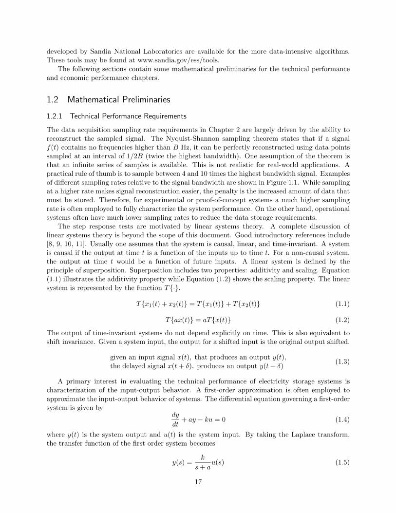
The data acquisition sampling rate requirements in Chapter 2 are largely driven by the ability toreconstruct the sampled signal. The Nyquist-Shannon sampling theorem states that if a signalf(t) contains no frequencies higher than B Hz, it can be perfectly reconstructed using data pointssampled at an interval of 1/2B (twice the highest bandwidth). One assumption of the theorem isthat an infinite series of samples is available. This is not realistic for real-world applications. Apractical rule of thumb is to sample between 4 and 10 times the highest bandwidth signal. Examplesof different sampling rates relative to the signal bandwidth are shown in Figure 1.1. While samplingat a higher rate makes signal reconstruction easier, the penalty is the increased amount of data thatmust be stored. Therefore, for experimental or proof-of-concept systems a much higher samplingrate is often employed to fully characterize the system performance. On the other hand, operationalsystems often have much lower sampling rates to reduce the data storage requirements.
The step response tests are motivated by linear systems theory. A complete discussion oflinear systems theory is beyond the scope of this document. Good introductory references include[8, 9, 10, 11]. Usually one assumes that the system is causal, linear, and time-invariant. A systemis causal if the output at time t is a function of the inputs up to time t. For a non-causal system,the output at time t would be a function of future inputs. A linear system is defined by theprinciple of superposition. Superposition includes two properties: additivity and scaling. Equation(1.1) illustrates the additivity property while Equation (1.2) shows the scaling property. The linearsystem is represented by the function T{·}.
T{x1(t) + x2(t)} = T{x1(t)}+ T{x2(t)} (1.1)
T{ax(t)} = aT{x(t)} (1.2)
The output of time-invariant systems do not depend explicitly on time. This is also equivalent toshift invariance. Given a system input, the output for a shifted input is the original output shifted.
given an input signal x(t), that produces an output y(t),the delayed signal x(t+ δ), produces an output y(t+ δ)
(1.3)
A primary interest in evaluating the technical performance of electricity storage systems ischaracterization of the input-output behavior. A first-order approximation is often employed toapproximate the input-output behavior of systems. The differential equation governing a first-ordersystem is given by
dy
dt+ ay − ku = 0 (1.4)
where y(t) is the system output and u(t) is the system input. By taking the Laplace transform,the transfer function of the first order system becomes
y(s) =k
s+ au(s) (1.5)
17

Figure 1.1: Data sampling rate requirements.
18

The step response of a first order system in the Laplace domain is
y(s) =k
s(s+ a)(1.6)
Taking the inverse Laplace transform yields the following time response
y(t) =k
a
(1− e−at
)(1.7)
By taking step response data, one can apply various methods (e.g. least squares, etc.) toestimate the first order approximation of system parameters from test data. Higher order modelscan be applied if a first order model is insufficient to capture the dominant system dynamics. It isoften common to fit a second order model given by
y(s) =ω2n
s2 + 2ζωs+ ω2n
u(s) (1.8)
Applying a step response input and taking the inverse Laplace transform yields the following timeresponse.
y(t) = 1− 1
βe−ζωnt sin(ωnβt+ θ), where β =
√1− ζ2, θ = tan−1
(β
ζ
)(1.9)
The transient response of a second order system is characterized by the damping ratio, ζ, whichprovides insight into the step response. For large values of ζ, the step response will be relativelyslow with no overshoot. As ζ is decreased, the response becomes quicker. For ζ = 0.7, the systemwill have a small overshoot. As ζ is decreased further, the response becomes quicker but moreoscillatory. If ζ becomes zero, the response will be purely oscillatory. Negative values will result inan unstable system with growing oscillations. This behavior is illustrated in Figure 1.2.
Key step response parameters include:
• Rise time, Tr
• Peak time, Tp
• Settling time, Ts
• Percent overshoot, P.O.
Referring to Figure 1.3, the percent overshoot is defined as
P.O. = 100(M − 1) (1.10)
Note that in this figure, the output value has been scaled so that the steady state value is 1.0. Thesettling time, Ts, is the time required to settle within +/−δ of the final value. The peak time, Tp isthe time required to reach the peak overshoot value. This parameter is not defined for well dampedsystems that do not have any overshoot. There are several common definitions of rise time, Tr. Inthis report, we recommend the time to reach 90% of the final value. Another common practice isto measure the time from 10% to 90% of the final value.
19

Figure 1.2: Step response of a 2nd order system.
Figure 1.3: Step response parameters.
20

1.2.2 Financial Calculations
In this section, we present the mathematical preliminaries for the financial calculations employedin this report. Many of these calculations are typical engineering economic analysis [3].
Project evaluation is the process by which information is organized to consistently and ob-jectively evaluate the economic merit of investments (the process of delaying current for futureconsumption) and is often referred to in the public sphere as benefit-cost analysis (B-C) and in theprivate sphere as discounted cash flow (DCF) analysis. The approaches are very similar thoughtheir main distinguishing feature is that the latter focuses on cash flows from the perspective of aprivate entity while the former likely also includes estimated benefits and costs that may not bereflected in explicit cash flows. The bottom line metric employed to determine whether the projectshould be undertaken is usually referred to as the investment criterion. A variety of such criteriaare available but most typically are net present value (NPV) (alternatively present value of net ben-efits) or benefit-cost ratio (B/C) 1. For a more detailed exposition of benefit-cost analysis and itsrelationship to discounted cash flow analysis see [1]. The following sections review the calculationsfor the time value of money, cost benefit analysis, and return on investment.
Time Value of Money
The so-called time value of money derives from a concept economists refer to as time preference.Human beings are somewhat myopic as evidenced by their preference for current consumption overfuture consumption; the rate at which this preference is expressed is referred to as the rate of timepreference and probably has its basis in uncertainty of the future as perceived by humans.
Money is the equivalent of consumption since it provides the holder with command over con-sumption goods. If an individual expresses indifference between receiving $1.00 now or $1.05 oneyear from now, this individual’s rate of time preference is 5% per annum. Individuals may eachhave different rates of time preference and, in a societal context, one can speak of the social rate oftime preference as the collective preference of a society for present over future consumption. Thesocial rate of time preference would be the rate at which society would judge long-lived projectsthat require the sacrifice of current consumption to provide greater consumption in the future.
Applying these concepts, the time value of money is the value of money at some date referencedto another date given the amount of interest earned over the time period. The choice of interest rateis dependent on the application. The Fisher equation estimates the relationship between nominaland real interest rates under inflation [12]. The nominal interest rate, i, is a function of the realinterest rate, r, and the inflation rate, π.
1 + i = (1 + r)(1 + π) (1.11)
i ≈ r + π (1.12)
The nominal interest rate is the market rate for a financial instrument. The interest rate employedis often the risk-free interest rate, which is the rate of return from an investment with no risk offinancial loss. The interest rate on short-term government bonds is often used as a proxy for therisk-free rate. The real interest rate measures the purchasing power of interest receipts adjustedfor inflation. When calculating the time value of money, a key question is what interest rate shouldbe used. If the analysis is attempting to take into account the effects of inflation, one should usethe nominal interest rate. This implies that one should make some effort to model inflation in the
1Others include internal rate of return, rate of return on investment, rate of return on assets, rate of return onequity. These are most often used in the private sector.
21

future. An alternative approach is to employ the real interest rate and to perform the analysis netof any price changes over time. A resource for identifying nominal and real interest rates is foundin [13]. All of the analysis in this report will employ real interest rates for evaluating the time valueof money.
If the real interest rate is 5% per year, $100 invested today will be worth $105 in 12 months.Likewise, if someone promises you a deposit of $105 12 months from now, the value of that todayis only $100. There are two ways to define the interest rate: simple interest or compound interest[3]. Simple interest is computed on the original sum, as shown below:
total interest earned = P × r × n (1.13)
where P is the original principal, r is the interest per period, and n is the number of periods. Fora loan, the amount due at the end (the future payment F ) is given by
F = P + Prn, or F = P (1 + rn) (1.14)
Compound interest is more prevalent than simple interest. Compound interest accrues on thecurrent balance at the end of each period. The future value F of a present sum P is given by
F = P (1 + r)n (1.15)
where n is the number of periods. Likewise, the present sum P in terms of the future value F is
P =F
(1 + r)n= F (1 + r)−n (1.16)
If the interest rate is defined with continuous compounding, the future value F at time T of apresent sum P is given by
F = PerT (1.17)
Likewise, the present value in terms of the future value is given by
P = Fe−rT (1.18)
When evaluating a potential stream of expenses and receipts over some period of time, thevalue of the payments and receipts must be referenced to some time in order to make a meaningfulassessment. It is typical to bring every cash flow back to present value, or to the value at the endof the project, in which case it is a future value. An example of calculating the present value ofa stream of receipts and expenses is shown in Figure 1.4. This approach is known as net presentworth (PW) analysis or net present value (NPV) analysis.
Present Worth Analysis
Present worth analysis, often referred to as net present value (NPV) analysis, calculates the presentvalue of all cash flows associated with a project. A negative cash flow is referred to as a disbursementor cost. A positive cash flow is referred to as a receipt or benefit. Cash flows are usually expressedin either table form or a cash flow diagram. An example of each appears in Figure 1.5. Net presentvalue is often applied as a criterion to select between mutually exclusive alternatives, where theproject with the highest NPV is selected. In cases where the benefits are the same for each project,it is sufficient to minimize the present worth of the costs. The present worth of the costs are oftenreferred to as the total life cycle costs (TLCC). Similarly, for cases where the input costs are thesame for each project, it is sufficient to maximize the present worth of the benefits.
22

6 6 6 6 6 6
? ? ? ? ? ?
?transmission line, T0
transmission tariff receipts, Ti
O/M Costs, OMi
0 1 2 3 4 5 oo Ntime (years)
NPV = −T0 −N∑i=1
OMie−rti +
N∑i=1
Tie−rti
Figure 1.4: Time value of money example, valuation of a series of cash flows. Continuous com-pounding.
Benefit-Cost Analysis
When a regulated, investor-owned utility (IOU) wishes to invest in an energy storage device, publicutility commissioners and their staffs should expect to receive an analysis of the investment ingrid assets in the form of a private benefit-cost analysis of the investment. This analysis couldtake a variety of forms, depending upon the preferred analysis approach of the particular utilitypresenting the analysis. Nevertheless some key elements should be incorporated. Foremost, theimportant issue of the perspective of the analysis should be addressed. The commission shouldexpect the regulated IOU to present an analysis from the perspective of their shareholders, withthe analysis demonstrating that the investment adds to shareholder value. This would be a privatebenefit-cost analysis. As such, it would contain evaluations of only benefits and costs as viewedfrom the utility’s perspective. Additional sales of electricity would be evaluated at the regulatedrates for the utility, and costs would be accounted from the point of view of the utility. Becauserates are regulated, the successful investment would be viewed as a reduction of costs compared tosome alternative. This would involve an analysis of at least two alternatives: the “undertake theproject” alternative and the “do not undertake the project” alternative.
With specific grid needs identified, and the EES technologies that can supply those needs alsoidentified as described, a benefit-cost evaluation process can be applied. While it is not the purposeof this report to develop a complete description of all of the issues relevant to the development of abenefit-cost analysis of a private project, a high-level description of the important methodologicalissues is appropriate and thus provided.
Benefit-cost analysis applied in a private sector context is often referred to as discounted cashflow (DCF) analysis [1]. The methodological principles and techniques of the two approachesare virtually the same. The main difference is that the private analysis focuses exclusively onthe revenue and cost (cash) flows that are estimated to result over the lifetime of the project
23

End of Year Cash Flow
0 -$10,0001 $8,0002 $7,0003 $15,000
6 6
6
?-$10,000
$8,000$7,000
$15,000
0 1 2 3
NPV = −$10, 000 +$8, 000
(1 + r)+
$7, 000
(1 + r)2+
$15, 000
(1 + r)3
Figure 1.5: Example cash flow table, cash flow diagram, and NPV calculation. Discrete compound-ing.
24
upon its implementation, and does not include public benefits and costs. Again, this is adoptingthe perspective of the investor in the EES system2. Additional analyses might accompany theinvestment proposal; for example, if the investor is the utility itself, it will also likely perform arevenue requirements analysis to demonstrate the likely impact of the investment on the need for orlack of need for retail electric rate adjustment. It is likely that a suite of analyses would support theproposal to the commission. A DCF/benefit-cost analysis to demonstrate positive net benefits overthe long term, helping to support the capacity adequacy aspect; a revenue requirements analysisto demonstrate retail rate impact, if any; and a production cost modeling exercise to demonstrateoperating cost-effectiveness. These are all likely components of the analysis suite.
It is possible that the commission or its staff will wish to extend this private benefit-cost analysisinto a consideration of the public benefits and costs of the project. In that case, much of the relevantinformation about the project will already be available from the private analysis.
A schematic representing the process of reaching a decision using the application of benefit-costanalysis is contained in Figure 1.6. This figure represents the allocation of resources to one or theother of two projects where the right hand branch represents alternatives (including doing noth-ing). The do nothing alternative should always be present in project comparisons. Independencebetween the benefits and costs of the projects is normally assumed. In a particular application, ifindependence is not the case, then additional alternatives must be devised that are comprised ofa combination of the interdependent projects. Incremental benefits and costs must then be calcu-lated for the combined alternative. The effect of the process described in Figure 1.6 is to apply theeconomic concept of opportunity cost. If resources are assumed scarce, the cost of action A is thenet revenue that could have been earned from applying the resources to action B instead. Otherreferences on benefit-cost analysis include [14] and [3].
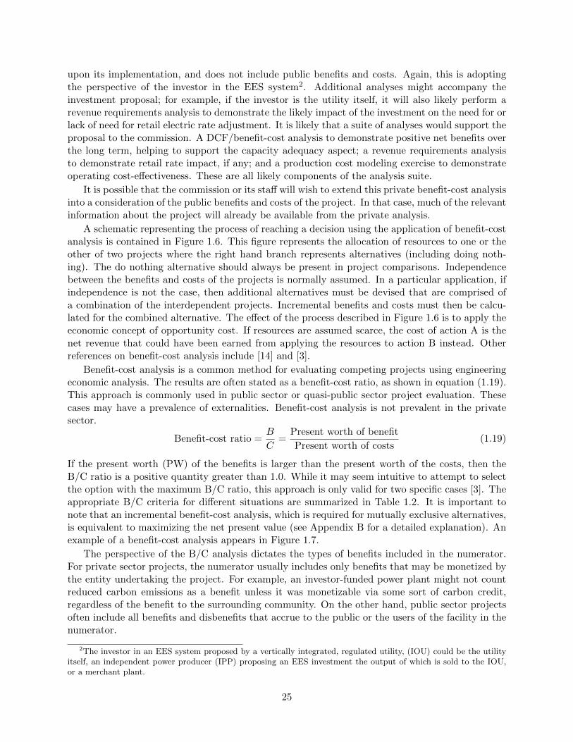
Benefit-cost analysis is a common method for evaluating competing projects using engineeringeconomic analysis. The results are often stated as a benefit-cost ratio, as shown in equation (1.19).This approach is commonly used in public sector or quasi-public sector project evaluation. Thesecases may have a prevalence of externalities. Benefit-cost analysis is not prevalent in the privatesector.
Benefit-cost ratio =B
C=
Present worth of benefit
Present worth of costs(1.19)
If the present worth (PW) of the benefits is larger than the present worth of the costs, then theB/C ratio is a positive quantity greater than 1.0. While it may seem intuitive to attempt to selectthe option with the maximum B/C ratio, this approach is only valid for two specific cases [3]. Theappropriate B/C criteria for different situations are summarized in Table 1.2. It is important tonote that an incremental benefit-cost analysis, which is required for mutually exclusive alternatives,is equivalent to maximizing the net present value (see Appendix B for a detailed explanation). Anexample of a benefit-cost analysis appears in Figure 1.7.
The perspective of the B/C analysis dictates the types of benefits included in the numerator.For private sector projects, the numerator usually includes only benefits that may be monetized bythe entity undertaking the project. For example, an investor-funded power plant might not countreduced carbon emissions as a benefit unless it was monetizable via some sort of carbon credit,regardless of the benefit to the surrounding community. On the other hand, public sector projectsoften include all benefits and disbenefits that accrue to the public or the users of the facility in thenumerator.
2The investor in an EES system proposed by a vertically integrated, regulated utility, (IOU) could be the utilityitself, an independent power producer (IPP) proposing an EES investment the output of which is sold to the IOU,or a merchant plant.
25

Accept project if $X >$Y
Project benefit = $X
Determine the value ofoutput from the project
Allocate scarceresources to the project
Undertake the project
Decision
Project opportunitycost = $Y
Determine the value ofoutput from resourcesin alternative projects
Allocate scarceresources to the
alternative projects
Do not undertake theproject
Figure 1.6: Benefit-cost analysis using the concept of opportunity cost [1].
26

6 6 6 6 6
? ? ? ? ?
?-$400
-$80 -$80 -$80 -$80 -$80
$160 $160 $160 $160 $160
0 1 2 3 4 5 time (years)
Given the cash flow above for a hypothetical project and a 7% cost of capital, the present worth ofthe benefits is calculated as
PW(B) = $160e−1(0.07) + $160e−2(0.07) + $160e−3(0.07) + $160e−4(0.07) + $160e−5(0.07) = $651.65
Similarly, the present worth of the costs is calculated as
PW(C) = $400 + $80e−1(0.07) + $80e−2(0.07) + $80e−3(0.07) + $80e−4(0.07) + $80e−5(0.07) = $725.82
The benefit-cost ratio is then calculated as
Benefit-cost ratio =PW(B)
PW(C)=
$651.65
$725.82= 0.8978
Since the benefit-cost ratio is less than 1.0, the costs outweigh the benefits and it would not beworthwhile to undertake the project.
Figure 1.7: Benefit-cost analysis example.
27

Situation Description Criterion
Variable inputsand variableoutputs
Inputs (e.g. money, etc.)and outputs (e.g. benefits)are variable.
Two alternatives: Compute the incrementalbenefit-cost ratio on the increment of invest-ment between the alternatives. If ∆B/∆C ≥1, select the higher cost alternative; otherwiseselect the lower cost alternative.
Variable inputsand variableoutputs
Inputs (e.g. money, etc.)and outputs (e.g. benefits)are variable.
Three or more alternatives: Solve by incre-mental benefit-cost ratio analysis.
Fixed input Inputs (e.g. money, etc.)are fixed.
Maximize B/C.
Fixed output Outputs (e.g. tasks, bene-fits, etc.) are fixed.
Maximize B/C.
Table 1.2: Benefit-cost analysis criteria for different scenarios [3].
Internal Rate of Return
Internal rate of return (IRR) is defined as the rate of return at which the present value of all cashflows is equal to zero [3]. When assessing the viability of a potential project, the internal rate ofreturn is compared to a minimum attractive rate of return (MARR). If the projected internal rateof return is less than the MARR, the project is not worth pursuing. Like benefit-cost analysis,rate of return analysis can also be employed to evaluate different alternatives. When there aretwo options, an incremental rate of return (∆IRR) is calculated on the difference between thealternatives. If the ∆IIR ≥ MARR, the higher cost alternative is selected. Otherwise, the lowercost alternative is selected. Figure 1.8 goes through an example rate of return calculation.
Levelized Cost of Energy
The levelized cost of energy (LCOE) is the cost assigned to every unit of energy produced (or saved)over the analysis period [6]. Thus, for each time interval corresponding to the unit of energy, thecost is equal to the LCOE times the quantity of energy. If each of these costs is discounted topresent value, the total cost should equal the total life cycle cost (TLCC). This yields the equationfor LCOE,
N∑i=1
Qi × LCOE
(1 + r)i= TLCC (1.20)
where Qi is the quantity of energy for period i, r is the interest rate for each period, and N is thenumber of periods. Similarly, the total life cycle cost is defined as
TLCC =N∑i=1
Ci(1 + r)i
(1.21)
28

6
6
66
6
?-$800
$180
$360
$180$60
$180
0 1 2 3 4 5 time (years)
The internal rate of return is calculated by solving for the interest rate which makes the presentworth of all cash flows equal to zero. For the cash flows shown above, the equation to solve is givenby
0 = −$800 + $180e−r + $360e−2r + $180e−3r + $60e−4r + $180e−5r
Solving for a closed-form solution is often very difficult, so internal rate of return calculations areusually solved with some sort of optimization routine, or by trial and error. Most financial softwarepackages have tools for estimating internal rate of return. Solving the equation above, the internalrate of return is 6.95% for this example.
Figure 1.8: Internal rate of return example.
29

where Ci is the cost associated with period i. Combining these two equations and solving for LCOEyields
LCOE =
N∑i=1
Ci(1 + r)i
N∑i=1
Qi(1 + r)i
(1.22)
Note that the quantity of energy Qi is not being discounted, the discounting factor in the numeratorand denominator are the result of combining equations (1.20) and (1.21).
1.3 Electricity Storage Model
Electrical Power Input Storage Device Electrical Power Output
• Electrical
• Chemical
• Mechanical
• Thermal
Figure 1.9: Electricity storage block diagram.
A block diagram representing an energy storage system is shown in Figure 1.9. The key param-eters that characterize a storage device are:
• Power Rating [MW]: the maximum output power of the storage device. We assume thatthe maximum discharge and charge power ratings have the same amplitude.
• Energy Capacity [Joules or MWh]: the amount of energy that can be stored.
• Efficiency [percent]: the ratio of the energy discharged by the storage system divided by theenergy input into the storage system. Efficiency can be broken down into two components:conversion efficiency and storage efficiency. Conversion efficiency describes the losses encoun-tered when input power is stored in the system. Storage efficiency describes the time-basedlosses in a storage system.
• Ramp Rate [MW/min or percent nameplate power/min]: the ramp rate describes howquickly the storage device can change the state of charge or discharge.
In order to facilitate financial analysis of an energy storage system providing one or several gridservices, a model of the system is required. A straightforward approach is to keep track of the energystored at the end of each time interval. This yields the following model to track the state-of-charge:
St = St−1 + γcqct − qdt − γsSt−1, (MWh) (1.23)
where
30

St Energy stored at the end of time period tSt−1 Energy stored at the end of time period t− 1γc Conversion efficiency (percent)qct Quantity of energy pulled from the grid (charge) during time period t (MWh)qdt Quantity of energy provided to the grid (discharge) during time period t (MWh)γs Storage efficiency (percent)
The model is intuitive. The current energy level is a function of the charge and discharge quantities,the conversion efficiency, the energy level at the previous time step, and the energy losses over thetime period. Additional parameters associated with the model are the length of the time period,the maximum charge/discharge quantities and the maximum storage capacity of the system. Thesequantities are defined as:
∆t time period (for example, hours)q̄D maximum quanitity that can be sold/discharged in a single period (MWh)q̄R maximum quantity that can be bought/recharged in a single period (MWh)S̄ maximum storage capacity (MWh)
Armed with a model for the system state of charge, it is straightforward to quantify the financialcosts/benefits associated with charging and discharging while engaging in a functional use. Therevenue at each time step is given by
Rt = qdt (P dt − Cdt )− qct (P ct + Cct ) (1.24)
where
P dt Price received for discharging at time period t ($/MWh)Cdt Cost for discharging at time period t ($/MWh)P ct Price paid for charging at time period t ($/MWh)Cct Cost for charging at time period t ($/MWh)
The present value of the energy storage system can be written as
Present Value =N∑t=1
(qdt (P dt − Cdt )− qct (P ct + Cct )
)e−rt (1.25)
Using this relationship, it is possible to calculate the present value of a system using either historicalor estimated price data under a wide range of scenarios. The charge/discharge quantities can bederived to maximize revenue (e.g. a linear programming optimization problem) or are generated bya candidate control algorithm. In a market area one can utilize historical price data. In a verticallyintegrated utility the most difficult task is estimating the appropriate prices and costs to use in themodel 3. An example of estimating the maximum potential revenue from participating in arbitrageand frequency regulation is described in [15].
The next chapter discusses the technical performance requirements for various grid services thatmay be provided by an electrical energy storage system.
3This is discussed further in Chapter 3
31

32

Chapter 2
Technical Performance Requirements
2.1 Introduction
Grid-connected energy storage systems have the potential to provide a variety of benefits. Thissection specifies the technical requirements a given storage system must meet in order to claim thesystem provides a given benefit. These requirements are broken down into four categories:
1. Specify requirements a storage system must meet to claim it provides a benefit.
2. Identify the engineering tests and analyses required to quantify the extent to which a givenstorage system provides a benefit.
3. Identify the technical data required to assess the benefits.
4. Make recommendations on what monitoring technologies are well suited to provide the re-quired data.
The framework for classification of the benefits of grid-connected storage was generally taken from[16, 17]. However, the goals of this report have a sharper technical focus. When viewing the benefitsdescribed in [16] with this focus, it became natural to re-group the benefits into a smaller set ofcategories. All benefits within a given category require similar technical assessment to measureachievement of the benefit. We form three broad categories along with sub-categories for thepurpose of assessing the technical requirements of grid-connected storage devices:
• Energy supply interactions
◦ Short-term energy shift
◦ Long-term energy shift
• Grid Operations
◦ Regulation and frequency control
◦ Voltage
◦ Power-factor control
◦ Angle stability control
◦ Sub-synchronous resonance
◦ Shedding (under frequency or under voltage)
33

• Quality and reliability
◦ UPS applications
◦ Harmonics
The engineering issues and time frames associated with each of these classes play a large part in dic-tating the technical requirements and monitoring needs. For example, sub-synchronous resonancehas a time-frame of milliseconds while long-term energy shift has a time frame of hours.
A grid-connected electric energy storage system includes the physical storage device, specificcontrols to operate the device, and external controls and equipment to connect and interact withthe grid and address the desired applications. The impact of a storage system on a particulargrid issue will involve a combination of the system’s inherent ability to respond to the issue, theexternal control system design and settings, and the location of the interconnection to the grid.Ideally, testing, assessment, and monitoring would be conducted to separate the response of theexternal controls from the inherent storage device response. In reality, this may not be possibledepending on the overall system design. The testing, assessment, and monitoring requirementsspecified in this document attempt to separate the responses of the fundamental storage device andthe external control system.
In an ideal setting, testing would be conducted to quantify the impact of the interconnectlocation. For example, a given storage system may have the inherent ability to supply a givenbenefit, but its particular interconnect location prohibits providing the benefit. An example of thismight be locating an energy storage device with the capability to mitigate harmonics in a “stiff”area of the bulk power grid that does not suffer from poor power quality. A device so locatedmay still provide myriad other benefits, but it cannot deliver the benefit of harmonic mitigationdue to its location on the grid. The testing, assessment, and monitoring requirements specified inthis document also attempt to separate the response of the fundamental storage system from anyfundamental limitations inherent from the interconnect location.
Energy storage technologies considered in this document include batteries, flywheels, pumpedhydro, compressed air, and any other technology that can store energy and that can be usedto provide system benefits when connected to the bulk power grid. Each of these technologieshas unique operation and control requirements. When interconnected to the grid, each will requireinterface through a three-phase synchronous connection. In order to provide grid benefits, a storagedevice must be equipped with customized control systems and interfacing equipment. The real-power injected into the grid must be a controllable variable. If the device is equipped with reactive-power control equipment, a second related settable variable must be provided. Set point optionsfor reactive power control may include one or more of the following:
• Voltage control - the terminal positive-sequence voltage magnitude;
• Power-factor control - the terminal power factor; or
• Reactive power control - the magnitude of the output reactive power.
Variables used in this report include the following.
• Possible inputs to the storage device are:
◦ Pset(t) = the set-point rms positive-sequence real power desired out of the device attime t. A negative Pset(t) refers to a device’s charging state.
◦ Pref (t) = the reference rms positive-sequence real power at time t. In many casesPset(t) is not equal to Pref (t) due to the frequency control system.
34

◦ Vref (t) = the reference rms positive-sequence voltage desired out of the device at time tassuming the device is equipped with reactive-power controls and operates in voltage controlmode.
◦ PFref (t) = the reference power factor desired at the device terminals at time t assumingthe device is equipped with reactive-power controls and operates in power-factor control mode.
◦Qref (t) = the reference rms positive-sequence reactive power desired out of the device attime t assuming the device is equipped with reactive-power controls and operates in reactive-power control mode.
◦ NOTE: only one of Vref , PFref , and Qref is possible for a given application.
• Outputs of the device are:
◦ P (t) = the true rms positive-sequence electrical real power out of the storage unit attime t, measured at the terminals of the storage device or at the utility point of interconnec-tion.
◦ Q(t) = the true rms positive-sequence electrical reactive power out of the storage unit attime t, measured at the terminals of the storage device, at the utility point of interconnection,or at some location remote from the storage device as required to achieve the desired effect.
2.2 Technical Categories and Benefits
As discussed above, a specific energy storage technology connected to the bulk electric power gridthrough a specific interface technology, for example a power electronic converter or a synchronousgenerator, placed at a specific location may not be capable of delivering a comprehensive rangeof benefits due to technical limitations. Similarly, this hypothetical storage device/grid interfacecombination placed at a specific location may not be capable of simultaneously delivering multiplebenefits to the grid due to technical and physical constraints. Therefore, for the purpose of mon-etizing the benefits provided by grid-connected storage systems it is appropriate to meticulouslydiscriminate between specific benefits so that they can be independently evaluated for the valuederived. However, this is not so for the purpose of evaluating the technical capability of a particularstorage technology to meet the desired benefit.
Table 2.1 describes a framework for further addressing the requirements for technical evalu-ation of the capability of an energy storage device to meet a given benefit. Benefits identifiedin [16] are categorized primarily according to the time frame required to implement a completecharge/discharge cycle while delivering the stated benefit.
It follows from the assignment of the three discussion categories shown in the table that certainmonitoring, data collection, analysis and evaluation methods and tools are applicable to certaincategories. The categories outlined in the table carry forward throughout the document.
2.3 Generic Data Collection Requirements
Table 2.2 is intended to describe broad categories of data acquisition and monitoring equipmentsuitable for use in collecting data for analysis within three monitoring classifications. Acronymsand abbreviations are further defined in the acronyms, abbreviations, and definitions section atthe beginning of the report. In Table 2.2 we attempt to describe classes of monitoring/informationsystems. These data/information source classes are then used as a guide for each benefit class
35

Table 2.1: Categories of benefits for technical evaluation.
Category name Mapping of benefit Designatorand description described in [16] in [16]
Energy supply interactions Short-term energy shift (minute time frame)Definition - Use of the energy • Renewable capacity firming 16storage device to support the • Wind generation grid integration 17“adequacy” of the supply-side Long-term energy shift (hour time frame)to meet the needs of the • Electric energy time-shift 1demand-side. “Adequacy” is a • Electric supply capacity 2term in common use in the • Electric supply reserve capacity 5industry and is defined in the • Transmission congestion relief 8glossary. • T&D upgrade deferral 9Time frame - Long. A single • Time-of-use energy cost management 11charge/discharge cycle may • Demand charge management 12take hours to complete. • Renewable energy time shift 15Sub-categories - Short-term • Increased asset utilization 18
(minutes); Long-term (hours). • Avoided transmission and distribution 19energy losses
• Avoided transmission access charges 20• Reduced transmission and distribution 21
investment risk• Dynamic operating benefits 22• Reduced generation fossil fuel use 24• Reduced air emissions from generation 25
Grid operations Regulation and frequency controlDefinition - Use of the energy • Load following 3storage device to support the • Area regulation 4real-time control of the electric Voltage controlpower grid. • Voltage support 6Time frame - moderate to • Transmission voltage support - voltage stability 7short. A charge/discharge cycle Power factor controlmay take seconds or, at the • Power factor correction 23most, minutes to complete. Angle stability controlSub-categories - Regulation • Transmission support - transient and 7
and frequency control; voltage small-signal stabilitycontrol; power factor control; Sub-synchronous resonanceangle stability control; sub- • Transmission support - sub-synchronous 7synchronous resonance; resonanceshedding. Shedding (under frequency or voltage)
• Transmission support - shedding 7
36

Table 2.1: Categories of benefits for technical evaluation (continued).
Category name Mapping of benefit Designatorand description described in [16] in [16]
Quality and reliability UPS applicationsDefinition - Use of the energy • Electric service reliability 13storage device to support the Harmonicsquality and/or reliability of • Electric service power quality 14energy delivered to the end-use.Time frame - Short. A singlecharge/discharge cycle may beon the order of milliseconds.Sub-categories - UPS
applications; harmonics.
to define data needs for future analysis. Some key points with respect to all data/informationcollection systems are shown below.
• All monitoring should be time-tagged. The accuracy of the time tag may vary with eachmonitoring class, but all measurements need to be capable of being correlated with oneanother. Some common difficulties with respect to time-tagging are time zone errors, daylightsavings time conversions, inaccurate and uncalibrated1 clocks, and other sources of error. Itis recommended that all data acquisition systems use the GMT (Greenwich Mean Time) timezone for all tagging.
• All monitored signals should have a bandwidth commensurate with the sample rate. Thisincludes all components of the data acquisition system, from sensor to transducer to sampler.For example, a band-limited transducer must not be used in a high sample rate application.As a rule of thumb, the chain of components comprising the entire measurement system shouldhave a bandwidth of approximately 1/4 of the sample rate (for example, the components of asystem sampling at 30 sps should have a bandwidth of 7.5 Hz). This is typical of most dataacquisition systems.
• The sampler should have an adequate dynamic range to cover all expected operating con-ditions. In the simplest example, a power transducer used to measure both charging anddischarging of a storage system should have the same range in both the positive and negativedirection.
Table 2.3 shows examples of data acquisition systems in each of the classes listed in Table 2.2.The examples are not meant to be prescriptive, nor are they representative of the entire range ofacceptable monitoring equipment. The examples are for illustrative purposes only. They do notform an endorsement or recommendation for a particular device or manufacturer. Even a cursoryreview of the literature will reveal that there are many available options and that there is muchoverlap between the technology categories described in this report.
1The calibration source should be commensurate with the required accuracy of the time tag.
37
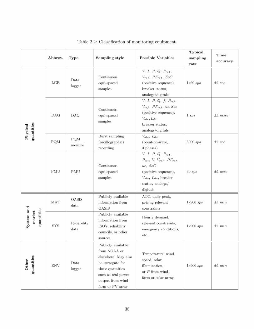
Table 2.2: Classification of monitoring equipment.
Abbrev. Type Sampling style Possible Variables
Typical
sampling
rate
Time
accuracy
Physical
quantities
LGRData
logger
Continuous
equi-spaced
samples
V, I, P, Q, Pref ,
Vref , PFref , SoC
(positive sequence)
breaker status,
analogs/digitals
1/60 sps ±1 sec
DAQ DAQ
Continuous
equi-spaced
samples
V, I, P, Q, f, Pref ,
Vref , PFref , ue, Soc
(positive sequence),
Vabc, Iabc
breaker status,
analogs/digitals
1 sps ±1 msec
PQMPQM
monitor
Burst sampling
(oscillographic)
recording
Vabc, Iabc
(point-on-wave,
3 phases)
5000 sps ±1 sec
PMU PMU
Continuous
equi-spaced
samples
V, I, P, Q, Pref ,
Pset, U, Vref , PFref ,
ue, SoC
(positive sequence),
Vabc, Iabc, breaker
status, analogs/
digitals
30 sps ±1 usec
System
and
mark
et
quantities
MKTOASIS
data
Publicly available
information from
OASIS
ATC, daily peak,
pricing relevant
constraints
1/900 sps ±1 min
SYSReliability
data
Publicly available
information from
ISO’s, reliability
councils, or other
sources
Hourly demand,
relevant constraints,
emergency conditions,
etc.
1/900 sps ±1 min
Oth
er
quantities
ENVData
logger
Publicly available
from NOAA or
elsewhere. May also
be surrogate for
these quantities
such as real power
output from wind
farm or PV array
Temperature, wind
speed, solar
illumination,
or P from wind
farm or solar array
1/900 sps ±1 min
38

Table 2.3: Examples of monitoring equipment.
Type Examples
Logger Shark 200S (www.electroind.com)
DAQ NI CompactDAQ (www.ni.com)
Phoenix Contact EMpro MA600 (www.phoenixcontact.com)
PMU SEL 351 (www.selinc.com)
ABB RES521 (www.abb.com)
PQ Monitor AEMC PowerPad (www.aemc.com)
Fluke 1740 (www.fluke.com)
GE F60 with DDFR (www.gedigitalenergy.com/multilin)
OASIS Western OASIS nodes (www.tsin.com/nodes/wscc.html)
Market data from a participating host utility may also be a good source
Reliability ERCOT historical (http://www.ercot.com/gridinfo)
SCADA data from a participating host utility may also be a good source
2.4 Energy Supply Interactions
Energy supply interactions are broadly defined as slow exchanges of energy between the bulk electricsupply sources and the energy storage device. Energy supply interactions often occur when thereis a disparity between the current market price of electricity and the future expected market price.These interactions usually occur over periods of many minutes or hours.
It could be argued that every exchange of energy between the bulk power grid and the storagedevice meets this definition, however, as previously discussed, the primary differentiator betweenthis definition, and that of the Grid Operations category and the Quality and Reliability categoryis the speed with which the storage device is required to operate.
The energy supply interactions category encompasses the majority of the specific benefits at-tributable to a stationary storage device. Two sub-categories can be identified, as described inTable 2.1, to provide more definition to the technical requirements placed upon a storage deviceproviding benefits in this category.
2.4.1 Short-term energy shift (minute time frame)
Short-term energy shift primarily encompasses the benefits associated with the use of storage tobalance renewable energy generation sources. It could also be argued that some of the valueattributable to “Dynamic Operating Benefits”, as described in [16], may also be captured in thissub-category.
Short-term energy shift is characterized by a storage device’s application as a “firming” sourceto allow a piece of generating equipment to be scheduled as a firm resource. New schedules for thegeneration fleet have historically been posted hourly, but with the increasing levels of renewableenergy, transmission operators are now implementing sub-hourly dispatch of generation. Therefore,for a storage device to offer an effective service in this category the device must be capable ofroutinely providing real power injections in a time frame of minutes and must sustain these realpower injections for periods of up to one hour.
There is now considerable data available regarding the variability of wind and solar power
39

Table 2.4: Wind power plant variability [4, 5].
PlantCapacity(MW)
Maximum1-minutechange(MW)
97.5% of1-minute
changes areunder (MW)
Maximum10-minute
change(MW)
97.5% of10-minute
changes areunder (MW)
358.5 N/A 8 112 30741 136 11 210 47895 116 9 202 401445 149 12 208 561450 158 20 314 741994 222 14 259 70
plants. Two studies performed in the northern Rocky Mountains serve to illustrate the issue forwind power plants [4, 5]. Summary data from these studies is shown in Table 2.4. It must benoted that variability is not the key factor in determining the value from a short-term energy shift.Rather, the key factor is the amount of deviation from the generation forecast for the wind/solarpower plant. Nevertheless, if a storage device is to perform the function of smoothing variabilityfrom an intermittent generating source to “firm” the source then the storage device must have thetechnical capability to track the generating source’s variability.
In order to attempt to quantify the technical requirements for a device claiming a short-termenergy shift benefit, one might express the results of Table 2.4 as a percent of the nameplate capacityof the renewable energy source. A rule-of-thumb requirement using this approach might state thatthe storage device must be capable of ramping at a rate of 12%2 of the nameplate capacity perminute for the generation resource deriving the benefit. Similar rules-of-thumb could be derivedfor ramp rate requirements to meet solar photovoltaic power plants.
Unlike the requirements for Grid Operations and Quality/Reliability described below, someshort-term energy shift benefit can be realized from any reasonable ramp rate provided by thestorage device. For example, if a wind power plant sees a sudden decrease of 100 MW in oneminute due to some peculiar weather event and a storage device responds at a rate of 10 MW perminute a certain amount of benefit is still realized. This makes it difficult to quantify absoluterequirements for storage devices claiming a short-term energy shift benefit. However, it shouldsuffice to assert that some storage technologies may be too slow to capture the full value of thebenefit, but any storage device having a reasonable capacity should be able to provide some degreeof benefit in this sub-category.
The task of validating that a storage device is providing short-term energy shift benefits maybe easier than the task of quantifying performance requirements for the same sub-category. Figure2.1 shows a block diagram of a generalized set point controller using remote measurements. Forexample, the remote measurements may be transmitted to the storage device from a wind powerplant. The variables include:
• t = time.
• Pref (t) = the reference rms positive-sequence real power at time t (this value may, for exam-ple, be the scheduled value for the wind power plant as communicated from the area control
212% is approximately the average of the maximum 1-minute deviations from the table.
40

P (t)
Telemeteredfrom renewableresource
+
-
Pref (t)
Pset(t)
a
b
c
Grid
RealPowerSensor
StorageDevice
ControlBlock
P (t)
Figure 2.1: Generalized set point controller using remote measurements.
center).
• Pset(t) = the set-point rms positive-sequence real power desired out of the device at time t.
• P (t) = the true rms positive-sequence electrical real power out of the storage unit or out ofthe renewable resource power plant at time t.
• abc =three-phase electrical connection to grid.
The ramp rate of the storage device may be determined by inputting a step-change at Pset(t)and subsequently measuring the output of the storage device at P (t). As discussed previously, moststorage technologies will not be rate-limited with respect to this benefit sub-category.
To determine the value delivered, the analyst must have access to the generation forecast forthe renewable resource benefited, the real power output from the renewable resource benefited,the real power output from the storage device, and the locational price of energy. Each of theseanalysis variables must be recorded and stored as a time history. Because of the long time constantsinvolved in this application it will be necessary to collect months, if not years, of data to obtainstatistically meaningful analysis results. Data should be collected at a sampling rate of one sampleper minute (1/60 sample per second) for variables over which the analyst has control (for example,P (t)). For variables over which the analyst does not have control, such as price of energy, datashould be stored at the fastest rate offered by the controlling agency.
A simple data logger should be sufficient to record the electrical variables, though a SCADAsystem is preferred. Price and forecast information can be collected from the appropriate sourcevia a network connection and recorded with a time stamp in the data repository.
2.4.2 Long-term energy shift (hour time frame)
Long-term energy shift involves storing energy when there is excess supply capacity and injectingenergy when there is high demand. In most cases the signal indicating the conditions of supplyand demand will be a price signal, but other indicators are also possible. Arbitrage as defined in[16], is one form of long-term energy shift.
It should be noted that excesses or shortages in electric energy supply may, in some cases, belocalized. This can occur when a geographic area is constrained by the capacity of the transmission
41

X(t)
Telemeteredfrom remoteresource
Pset(t)
a
b
c
Grid
RealPowerSensor
StorageDevice
ControlBlock
P (t)
χ(t)
External output
Figure 2.2: Generalized controller for long-term energy shift.
system connecting a “load pocket” to the rest of the bulk power grid. In all cases, long-term energyshift involves very slow charge/discharge cycling of the storage system.
The technical requirements, technical performance validation and monitoring requirements forlong-term energy shift are identical to that of short-term energy shift with one exception. Thesample rate of the monitored variables can be slower for long-term energy shift than for short-term,and the analyst may find it to be prudent to use averaging or some form of moving average (MA)filter on the measured variables before storing them to the data archive. From a signal processingperspective, an anti-aliasing filter would achieve the same goal. A common form of averaging forthis kind of data collection is to record the average P (t) in 15-minute blocks with no overlap. Itis important to note that although the data is recorded at a relatively slow rate, the quantity ofinterest must be sampled at a higher rate and then filtered. Otherwise, information is lost (forexample, the case where P (t) is sampled once every 15 minutes).
Figure 2.2 shows a block diagram of a generalized controller for long-term energy shift. Thevariables include:
• t = time.
• Pset(t) = the set-point rms positive-sequence real power desired out of the device at time t.
• P (t) = the true rms positive-sequence electrical real power out of the storage unit or out ofthe renewable resource power plant at time t.
• X(t) = an external input, often the price of energy at time t, used to affect control of thestorage device.
• χ(t) = an external output from the grid at time t that is to be used to assess the valueof the benefit derived. An example might be the CO2 emissions from a power plant thatwas formerly operating in “load following” mode but that is now, due to the storage device,operating as a “base load” unit.
• abc = three-phase electrical connection to grid.
P (t) should be sampled at least as frequently as the update rate on the price signal, or othersignal, used in the decision logic for the benefit being analyzed.
42

2.5 Grid Operations
Grid operations may include both transmission and distribution operations practices. The mostcomplex analyses involve real power dispatch and automatic control operations for transmissionoperations. Distribution operations are more closely connected to maintaining an acceptable voltageprofile and dispatching reactive power.
While energy supply interactions involve relatively long time frames, some of the grid operationsfocus areas are quite fast, with commensurately fast monitoring requirements. For this reason, thefollowing sections provide more depth than the previous ones.
In many cases, there are no clearly defined requirements that a generic device (including genera-tors) must meet to claim it supports a given grid issue. The requirements specified in this documenttake a conservative view. That is, if a storage device meets the requirements specified below fora given issue, then assuredly the device can claim it serves that issue. But, if the device does notmeet the requirements, it may still help in the given issue depending on the extent to which therequirements are not met.
2.5.1 Regulation and frequency control
As referenced in [16], the term “Regulation” refers to the control of a storage device as part of anArea Generation Control (AGC) system. Traditionally, each control area within a grid periodicallysends a reference power (Pref ) to key swing generators. A component of Pref is calculated withthe goal of driving the Area Control Error (ACE) to zero. The ACE is a combination of tie-linepower flow errors and frequency error for the control area of interest.
AGC is only one of two power-system components focused on frequency control and load balanc-ing (excluding under-frequency load shedding). Power-system frequency control is usually brokeninto primary and secondary control [2]. Primary control relates to how the system immediatelyreacts to a sudden disturbance (such as a generator trip) over the first several seconds and is mainlya function of the automatic speed-governor control systems on key generators within the system.Often, speed governor controllers are operated with a dead-band, so they are only activated undersevere system conditions. Secondary control relates to several minutes after primary control andis primarily a function of the AGC system’s reaction to the disturbance. In reality, the dynamicdivision between primary and secondary frequency response is somewhat fuzzy. It depends onmany factors including the bandwidth of the control systems and controlled devices (for example,generation and storage).
The Regulation definition in [16] is expanded to include both frequency control components.Regulation is typically incorporated into a generation device (and expectedly a storage device)through combination with a “speed governing” control system – a frequency-based feedback controlsystem. Therefore, monitoring a storage device’s participation in Regulation cannot be separatedfrom the traditional speed-governing control. Figure 2.3 shows a block diagram of a generalizedspeed-governing/Regulation control system. The variables include:
• t = time.
• fref = desired electrical frequency at the grid connection (60 Hz).
• f(t) = actual fundamental frequency measured at the grid connection at time t.
• fe(t) = frequency error at time t.
• u(t) = output of Speed Governor Control Block at time t.
• Pref (t) = the reference rms positive-sequence real power at time t (for units participatingin Regulation, this value is communicated from the area control center (for example, an ISO)).
43

fref =60 Hz
+ fe(t) u(t)
+
Pref (t)
+
Pset(t)
a
b
c
f(t)
P (t)
-
RealPowerSensor
SpeedGovernorControl
ControlBlock 2
StorageDevice
ElectricalConnection
Grid
FrequencySensor
Figure 2.3: Generalized speed-governor/Regulation control system used to set Pset(t).
• Pset(t) =the set-point rms positive-sequence real power desired out of the device at time t.
• P (t) = the true rms positive-sequence electrical real power out of the storage unit at time t.
• abc = three-phase electrical connection to grid.
Performance and design of control systems is beyond the scope of this document. But, thehigh-level fundamental goal is to have P track Pset. Normally in steady-state Pset = Pref + u.The signal u(t) contains the frequency bias of Speed-Governor Control Block. There are severalvariations of the control system; but, all follow the general format shown in Figure 2.3 . The sensorfor P is shown high-lighted in yellow as it is not necessary for operation of the control system; but,it is necessary for monitoring the storages device’s frequency control ability.
It is possible that a device will not be equipped with the Speed-Governor Control block and thecorresponding frequency feedback. In this case, the Speed-Governor Control Block is not includedand Pref directly feeds into Control Block 2.
One goal in testing and assessing a storage device’s participation in frequency control is toseparate the response of the control system from the device. Using Figure 2.3 as an example,the goal is the study of the response from Pset to P . This will necessarily require disabling somecomponents of the external control system during testing. For example, the external control systemis disconnected at Pset and test signals are driven into the storage device. Other tests will requiretesting the device in conjunction with the control system.
Testing and assessing a storage device requires monitoring for both primary and secondaryfrequency response. In general, this requires assessing how well P tracks Pset both in open loopand closed loop configurations. Testing involves inputting test signals in the form of step functionsand ramps into Pset and/or Pref and measuring the corresponding response at P . These tests mustbe conducted with the device grid connected and operating under all possible allowed charge states.
44

Figure 2.4: The sequential actions of primary, secondary, and tertiary frequency controls followingthe sudden loss of generation and their impacts on system frequency. Taken from reference [2].
In typical AGC systems, Pref is updated every few seconds (for example, every 4 seconds). Theresponse time of the storage device to these changes provides assessment of the device’s ability toparticipate in Regulation. No standard requirements exist for the response time; but, a responsetime on the order of one minute is fairly standard.
Figure 2.4, which is taken from [2], is demonstrative of a typical system response to a largegenerator trip. Immediately after the generator trip, frequency starts to fall. Generators equippedwith speed-governor controls immediately start to raise their power output. If the system is stable,frequency reaches a minimum (termed the nadir point) and then starts to recover. Due to thedroop designed into the speed-governor controls, the frequency initially recovers to a level belowthe rated (60 Hz) and the recovery occurs within about 30 seconds. The secondary controls (AGC)then further adjust generator outputs to bring the frequency back to 60 Hz over the subsequentseveral minutes.
After a major frequency event, many of the power outputs of controlled generators are out ofbounds. In many cases, the generator reserves (the portion held back for speed governor and AGCactions) are consumed. The“Tertiary” control refers to the centrally coordinated actions to restoregenerator reserves back to a level to accommodate another major event. They provide a generalguideline of how long a storage device must sustain response as a secondary control device.
Frequency Control Tests, Monitoring, and Requirements
Table 2.5 and Table 2.6 summarize the tests, monitoring, and requirements for primary frequencycontrol and secondary frequency control, respectively. Each condition (primary and secondary)specify three tests. For both conditions, the goal of Test 1 is to evaluate the storage device separatelyfrom the control system. In addition, Tests 2 and 3 evaluate the entire “storage system;” that is,
45

the storage device operating with the control system active and the system synchronized to thegrid. It is recommended that all three tests be conducted under a variety of charge and dischargestates to demonstrate the limits of operation. That is, show when and how the storage systemswitches out of frequency control.
2.5.2 Voltage Control
The primary purpose of a voltage control application is to help maintain grid reliability. Voltagesupport and control can be broken into two categories: transient response and steady-state response.Transient response relates to how fast the device can provide reactive power to the grid following afault in order to maintain transient stability. Transients can be very fast with first-swing dynamicsmeasured in the sub-second range. Steady-state response relates to the constant voltage conditionunder ambient conditions. Both are critical to the reliability of a grid.
Traditionally, voltage support is broken into transmission level control and distribution levelcontrol. The transient requirements are supplied by the transmission system via generator con-trols, and fast-acting reactive devices including Flexible AC transmission system (FACTS) devices.Steady-state voltage support is provided at both the transmission level and the distribution level.The primary distribution level device is the tap-changing transformer.
Assuming a storage device is equipped with voltage control capability, the response and abilityof the device to control voltage is highly dependent on the external control system and equipment.Many equipment and interface strategies are possible and many may not be disclosed to the end user.Therefore, we propose testing and assessing voltage support benefits using a black-box approach.The testing and assessment must also consider if the support is transient and/or steady state.
A storage device operating under voltage control will effectively vary the output reactive powerto obtain the desired terminal voltage. A high-level perspective of the control system is shown inFigure 2.5. Variables include:
• t = time.
• Pset(t) = the set-point rms positive-sequence real power desired out of the device at time t.
• Vref (t) = the reference rms positive-sequence voltage desired out of the device at time t.
• ue(t) = the control signal transferred to the storage device from the Voltage Control block.Often termed the excitation signal. The unit and form of this signal depends on the reactivepower handling equipment employed by the storage unit.
• abc = three-phase electrical connection to grid.
• Va(t), Vb(t), Vc(t) = rms three-phase voltage magnitudes at the terminals of the storage unit(may be line-to-line or line-to-neutral) at time t.
• V (t) = rms positive-sequence voltage at the terminals of the storage unit at time t.
• P (t) = the true rms positive-sequence electrical real power out of the storage unit at time t.
• Q(t) = the true rms positive-sequence electrical reactive power out of the storage unit attime t.
A typical Power Control block is shown and defined in Figure 2.5. Performance and design ofthe Voltage Control block is beyond the scope of this document. The high-level fundamental goalis to have V track Vref . The sensors for P and Q are shown high-lighted in yellow as it is notnecessary for operation of the control systems, but, is necessary for monitoring the storage device’svoltage control ability.
46

Table 2.5: Primary frequency control tests, monitoring, and requirements.
TestNum
TestName
Test Description Monit’rdVar’s
Monitoring Requirements
1
StorageDevice,DirectRe-sponse(OpenLoop)
Open control loop atPset. Leave all othercontrol systems in placeand device connected togrid. Apply threeconsecutive step inputsseparated by 2 minuteseach to Pset. Thesecond step shall be inthe opposite directionof the first. Forexample, if the firststep is 20% full scale(FS) then the secondstep is -20% FS, andthe third 20% FS.
Pset, P ,Iabcphasors
PMU (5 spsminumum).Monitoringmust includeat least 5min. of dataprior to thefirst stepinput and 5min. afterthe thirdstep input.
P (t) must follow Pset(t) over theentire 16 min. For the 3 stepresponses, the system must meetthe following specs (see AppendixA under Step Response): Ts ≤ 10sec. and % OS < 10%Must meet above specs underboth charge and discharge condi-tions.P (t) must have a resolution of10% or less of rated output.A variety of step input ampli-tudes shall be tested and mustinclude a step input of 10% and100% of full scale in both chargeand discharge.Iabc must remain balanced duringtransients.
2
System,ActiveRe-sponse(ClosedLoop)
With the controlsystem active and thedevice connected to thegrid, set Pref to zero.Apply three consecutivestep inputs at fref ,each separated by 2minutes. The secondstep shall be in theopposite direction ofthe first and the third.
P ,Pref ,fref , f ,Iabcphasors
PMU (5 spsminumum).Monitoringmust includeat least 5min. of dataprior to thefirst stepinput and 5min. afterthe thirdstep input.
P (t) must follow fe(t) over theentire 16 min. with appropriatedroop scaling. For the 3 step re-sponses, the system must meetthe following specs (see AppendixA under Step Response): Ts ≤ 10sec. and % OS ≤ 10%If P (t) saturates, it must remainsaturated until the control de-mands a lower value.Must meet settling time underboth charge and discharge condi-tions.P (t) must have a resolution of10% or less of rated output.A variety of step input ampli-tudes shall be tested and must in-clude a step input of 0.01 Hz and0.1 Hz.Iabc must remain balanced duringtransients.
3
System,PassiveRe-sponse(ClosedLoop)
Actively monitorsystem during gridinterconnect. Capturesignificant frequencyevents within thesystem as well as thedevice’s response.
P ,Pref , f ,Iabcphasors
PMU (5 spsminumum).Monitoringmust includeat least 5min. of dataprior to theevent and 5min. afterthe event.
P (t) must follow fe(t) with ap-propriate scaling over the entire10 min. with a maximum of 2 sec.delay measured at the frequencynadir.Events in both charge and dis-charge state must be captured.P (t) must have a resolution of10% or less of rated output.Iabc must remain balanced duringtransients.
47

Table 2.6: Secondary frequency control tests, monitoring, and requirements.
TestNum
TestName
Test Desc. MonitrdVar’s
Monitoring Requirements
1
StorageDevice,DirectRe-sponse(OpenLoop)
Open control loop atPset. Leave all othercontrol systems in placeand device connected togrid. Apply step inputsto Pset.
Pset,P
DAQ (1 spsminumum).Monitoringmust include atleast 5 min. ofdata prior tothe input and30 min. afterinput.
P (t) must follow Pset(t) over theentire 35 min. and respond witha settling time of 1 min. or lessto the step.Must meet settling time underboth charge and discharge con-ditions.P (t) must have a resolution of10% or less of rated output.A variety of step inputs shallbe tested and must include astep input of 10% and 50% offull scale in both charge anddischarge.
2System,ActiveRe-sponse(ClosedLoop)
With the controlsystem active and thedevice connected to thegrid, apply step inputsat Pref .
P ,Pref ,f
DAQ (1 spsminumum).Monitoringmust include atleast 5 min. ofdata prior toand 30 min.after input.
P (t) must follow Pref (t) −Droop ∗ fe(t) over the entire 35min. with appropriate scalingand have a settling time of 1min. or less.Must meet settling time underboth charge and discharge con-ditions.P (t) must have a resolution of10% or less of rated output.
3System,PassiveRe-sponse(ClosedLoop)
Actively monitorsystem during gridinterconnect. Capturesignificant frequencyevents within thesystem as well as thedevice’s response.
P ,Pref ,f
DAQ (1 spsminumum).Monitoringmust include atleast 5 min. ofdata prior tothe event and30 min. afterthe event.
P (t) must follow Pref (t) −Droop ∗ fe(t) with appropriatescaling over the entire 35 min.with a maximum of 10 sec. de-lay.Events in both charge and dis-charge state must be captured.P (t) must have a resolution of10% or less of rated output.
48

Vref (t)
+
Pset(t)
ue(t)
a
b
c
P (t)
Q(t)
-
V (t)
Va(t)
Vb(t)
Vc(t)
SpeedControl
VoltageControl
StorageDevice
ElectricalConnection
Grid
RealPowerSensor
ReactivePowerSensor
VoltageSensor
Figure 2.5: Generalized voltage control system.
Voltage Control Tests, Monitoring, and Requirements
As illustrated in Figure 2.5, testing and assessment of a storage device’s voltage support and controlrequires time-synchronized monitoring of Vref , Vabc, V , Pset, P , and Q with the system connectedto the grid. Two distinct sets of experiments are required: one to assess the transient performance,and one to assess the steady-state performance.
Details for the transient test are given in Table 2.7. The test involves applying step inputs atVref and measuring the system’s response with the control in operation and the system synchronizedto the grid. Several step inputs need to be applied under a variety of step sizes and charge/dischargestates. If the control is unable to drive the voltage to the desired level due to limitations from thegrid, then the output Q(t) should go to a saturation level and remain there until switching back tovoltage control. At least one step input should demonstrate this condition. The sample-rate andbandwidth of the monitoring needs to be set to capture the full response time of the device. Rateson the order of 30 sps are common.
Steady-state voltage control tests are given in Table 2.8. For the first test, the system is operatedwith the control systems active and synchronized to the grid. Step inputs are applied at Vref andthe response of the system is monitored. The second test consists of capturing events within thegrid and recording the storage system’s response.
2.5.3 Power Factor Control
Unlike voltage control, the primary benefit for power factor (PF) control is to correct the PF for thecustomer. Often the goal is to reduce energy costs for the customer. Under such conditions, thereis no desire for transient response capability as with voltage control. Monitoring would thereforebe very similar to monitoring steady-state voltage control. An additional benefit is an increase inavailable transmission capacity. Higher real power levels can be achieved while still meeting the
49

Table 2.7: Transient voltage control tests, monitoring, and requirements.
TestNum
TestName
Test Desc. Monit’rdVar’s
Monitoring Requirements
1
System,ActiveRe-sponse(ClosedLoop)
With the controlsystem operating andthe device connected tothe grid, apply stepinputs at Vref .
P , Pset,Q,Vref ,V , Vabcphasors
PMU (30 spsminumum).Monitoringmust includeat least 1min. of dataprior toinput and 5min. afterinput.
V (t) must follow Vref (t) over theentire 6 min. and have a settlingtime of 1 sec. or less. This re-quirement only applies for caseswhere Q(t) does not reach a limit.For the above requirement, ifQ(t)reaches a limit then Q(t) must re-main at the limit until the de-mand allows for switching backto voltage control. The switchingcan be demonstrated by compar-ison of Vref and V (t).Must meet settling time for avariety of charge and dischargestates.Q(t) must have a resolution of10% or less of rated output.A variety of step inputs shall betested and must include a step in-put of 1% and 10% change in volt-age. At least one step shall drivethe system into Q(t) saturation.P (t) must remain at Pset(t) dur-ing tests. Pset(t) shall not varywith the step in the Vref com-mand.Vabc must remain balanced duringtransients.
50

Table 2.8: Steady-state voltage control tests, monitoring, and requirements.
TestNum
TestName
Test Desc. Monit’rdVar’s
Monitoring Requirements
1
System,ActiveRe-sponse(ClosedLoop)
With the controlsystem operating andthe device connected tothe grid, apply stepinputs at Vref .
P , Pset,Q,Vref ,V , Vabcphasors
DAQ (1 spsminumum).Monitoringmust includeat least 5min. of dataprior toinput and 30min. afterinput.
V (t) must follow Vref (t) over theentire 35 min. and have a settlingtime of 1 min. or less. This re-quirement only applies for caseswhere Q(t) does not reach a limit.For the above requirement, ifQ(t)reaches a limit then Q(t) must re-main at the limit until the de-mand allows for switching backto voltage control. The switchingcan be demonstrated by compar-ison of Vref and V (t).Must meet settling time for avariety of charge and dischargestates.Q(t) must have a resolution of10% or less of rated output.A variety of step inputs shall betested and must include a step in-put of 1% and 10% change in volt-age. At least one step shall drivethe system into Q(t) saturation.P (t) must remain at Pset(t) dur-ing tests. Pset(t) shall not varywith the step in the Vref com-mand.Vabc must remain balanced duringtransients.
2
System,PassiveRe-sponse(ClosedLoop)
Actively monitorsystem during gridinterconnect. Capturesignificant voltageevents within thesystem.
Q,Vref ,V , Vabcphasors
DAQ (1 spsminumum).Monitoringmust includeat least 5min. of dataprior toinput and 30min. afterinput.
V (t) must follow Vref (t) over theentire event and with a minimum1 min. delay. This requirementonly applies for cases where Q(t)does not reach a limit.For the above requirement, ifQ(t)reaches a limit then Q(t) must re-main at the limit until the de-mand allows for switching backto voltage control. The switchingcan be demonstrated by compar-ison of Vref and V (t).Events in both charge and dis-charge states must be captured.Q(t) must have a resolution of10% or less of rated output.Vabc must remain balanced duringtransients.
51

MVA rating of the transmission system.
A storage device operating under PF control will effectively vary the output reactive power toobtain the desired PF. A high-level perspective of the control system is shown in Figure 2.6 whichis very similar to voltage control. Variables include:
• t = time.
• Pset(t) = the set-point rms positive-sequence real power desired out of the device at time t.
• PFref (t) = the reference rms positive-sequence voltage desired out of the device at time t.
• ue(t) = the control signal transferred to the storage device from the PF Control block. Oftentermed the excitation signal. The unit and form of this signal depends on the reactive powerhandling equipment employed by the storage unit.
• abc = three-phase electrical connection to grid.
• Pe(t) = the true rms positive-sequence electrical real power out of the storage unit at time t.
• Qe(t) = the true rms positive-sequence electrical reactive power out of the storage unit attime t.
• PFe(t) = the PF measured somewhere in grid near the terminals of the device at time t.
A typical Power Control block is shown and discussed in Section 2.5.1. Performance and designof PF Control block is beyond the scope of this document. The high-level fundamental goal is tohave PFe(t) track PFref (t). The sensors for Pe(t) and Qe(t) are shown highlighted in yellow as itis not necessary for operation of the control systems, but, is necessary for monitoring the storagedevice’s PF control ability.
Using Figure 2.6 as a reference, tests, monitoring, and requirements are provided in Table 2.9.Two tests are recommended. The first is an active test involving placing step inputs into the PFrefcommand. A variety of step sizes and conditions should be tested. The second test is a passive onethat involves capturing grid events. Events can include times of significant power changes such asplanned ramps for the storage system.
2.5.4 Angle Stability Control
Angle stability relates to the electromechanical dynamic response of the system. It can focus onthe transient stability of a given generator or sets of generators, or on the steady-state stability ofthe overall system. A given storage device’s impact on angle stability is highly dependent on thedevice’s location within the grid, the devices inherent capability, and the device’s control system.Also, the assessment can be very complicated and time consuming. Entire multi-year studies areoften employed to assess a device’s impact on stability.
Monitoring and testing for angle stability applications is therefore extensive. Experimentswould involve measuring and analyzing transfer functions and responses of the device to majorfaults for several system and device operating conditions. The variables monitored highly dependon the control system being employed. At minimum, time-synchronized sample rates near 30 spsare required. All device output variables (P, Q, f, V, Vabc) and all controlled variables must bemonitored (for example, Pref , Pset, Vref , u, ue).
As an alternative, we propose tests on the storage system to assess its potential to impact anglestability if it were located at a favorable location. That is, we will not test the impact on stabilitydirectly; but, will test the ability of the storage system to impact stability if it were to be placedin a location with a control system that could impact stability.
52

Table 2.9: Power factor control tests, monitoring, and requirements.
TestNum
TestName
Test Desc. Monit’rdVar’s
Monitoring Requirements
1
System,ActiveRe-sponse(ClosedLoop)
With the controlsystem operating andthe device connected tothe grid, apply stepinputs at PFref .
P , Pset,Q,PFref ,PF ,Vabcphasors
DAQ (1 spsminumum).Monitoringmust includeat least 5min. of dataprior toinput and 30min. afterinput.
PF (t) must follow PFref (t) overthe entire 35 min. and have a set-tling time of 1 min. or less. Thisrequirement only applies for caseswhere Q(t) does not reach a limit.For the above requirement, ifQ(t)reaches a limit then Q(t) must re-main at the limit until the de-mand allows for switching backto voltage control. The switchingcan be demonstrated by compar-ison of PFref and PF (t).Must above 2 requirements for avariety of charge and dischargestates.Q(t) must have a resolution of10% or less of rated output.A variety of step inputs shall betested and must include a “small”change and a “large” change, anda change large enough to drive thesystem into Q(t) saturation.P (t) must remain at Pset(t) dur-ing tests. Pset(t) shall not varywith the step in the PFref com-mand.Vabc must remain equal in magni-tude, within the limits of the gridat the installation location.
2
System,PassiveRe-sponse(ClosedLoop)
Actively monitorsystem during gridinterconnect. Capturesignificant events withinthe system that createsignificant changes inimpedance at the pointof interconnection.
Q, P ,PF ,PFref ,Vabcphasors
DAQ (1 spsminumum).Monitoringmust includeat least 5min. of dataprior toevent and 30min. afterevent.
PF (t) must follow PFref (t) overthe entire event and with a mini-mum 1 min. delay. This require-ment only applies for cases whereQ(t) does not reach a limit.For the above requirement, ifQ(t)reaches a limit then Q(t) must re-main at the limit until the de-mand allows for switching backto voltage control. The switchingcan be demonstrated by compar-ison of PFref and PF (t).Events in both charge and dis-charge states must be captured.Q(t) must have a resolution of10% or less of rated output.Vabc must remain equal in magni-tude, within the limits of the gridat the installation location.
53

PFref (t)
+
Pset(t)
ue(t)
a
b
c
P (t)
Q(t)
-
PFe(t)
PowerControl
PowerFactorControl
StorageDevice
ElectricalConnection
Grid
RealPowerSensor
ReactivePowerSensor
PowerFactorSensor
Figure 2.6: Generalized power factor control system.
To favorably impact stability, a storage system must respond to a change in Pset and/or Qsetindependently. The response must be fast enough to impact the stability. Table 2.10 specifies twotests for P (t). If one is to consider using Q(t) as the controlled input to the grid, then these testsare conducted with inputs applied to Qset with Pset held constant. Note that the table refers toAppendix A for a more detailed description of the inputs.
2.5.5 Sub-synchronous Resonance
Resonance occurs when two or more components of a system interact with one another at a specificand unique frequency to create undamped oscillations. When this special frequency is excited byan outside source catastrophic failure of the system may occur. Both purely electrical and purelymechanical systems can exhibit resonance behavior. When these two systems are interconnected,the resonance frequencies may sometimes coincide. Such can be the case when a steam-poweredgenerator system (mechanical) interacts with a series compensated transmission line (electrical)resulting in a phenomenon known as sub-synchronous resonance (SSR).
As compared to hydro generators, steam-powered generator systems are normally designed tooperate at high mechanical speeds. Also, when compared to combustion turbine generating systems,steam plants typically have many more, and much heavier, masses connected to a single shaft. Asteam-powered generator assembly may consist of six turbine sections, a generator section, and anexciter section all on the same shaft and all spinning at 3600 rpm (angular shaft speed depends onthe number of poles in the machine). This complex mechanical system exhibits dynamic propertiesincluding several natural modes of oscillation.
Similarly, electrical resonance frequencies are established when inductive reactance and capaci-tive reactance both exist in the same electrical circuit. In reality, both inductance and capacitancealways exist in every electrical circuit. Usually the values are so small that the resultant resonance
54

Table 2.10: Angle stability control tests, monitoring, and requirements.
TestNum
TestName
Test Desc. Monit’rdVar’s
Monitoring Requirements
1
StorageDevice,DirectStepRe-sponse(OpenLoop)
Open any controlsystem such that Pset
and Qset can beindependently set.Apply step inputs toPset while holding Qset
constant.
Pset,Qset,P , Q,Vabcpha-sors,Iabcphasors
PMU (30 spsminumum).Monitoringmust includeat least 5min. of dataprior toinput and 5min. afterinput.
P (t) must follow Pset(t) over theentire 10 min. and must respondwith the following specs (see Ap-pendix A under Step Response):Tr < 115 millisec.; Ts < 630 mil-lisec. and % OS ≤ 10%Must meet settling time in bothcharge and discharge states.P (t) must have a resolution of 2%or less of full scale.P (t) must follow Pset(t) with asteady-state accuracy of 2% offull scale.A variety of step inputs shall betested and must include a step in-put of 10% and 100% of full scalein both charge and discharge.Q(t) must remain at Qset(t)within 5% of full scale.Vabc must remain equal in magni-tude, within the limits of the gridat the installation location.Iabc must remain equal in magni-tude, within the limits of the gridat the installation location.
2
StorageDevice,DirectAvail-abilityRe-sponse(OpenLoop)
Open any controlsystem such that Pset
and Qset can beindependently set.Conduct twoavailability tests (seeAppendix A), with Pset
as the input whileholding Qset constant.Test parameters are:fp = 0.8 Hz, 0.1 Hz;Amax
Amin= ±100% of FS,
+50% of FS; +10% ofFS; Amid = 0;Tc1 → Tc4 = 1 min.;Tp1 → Tp3 = 4 min.
Pset,Qset,P , Q
PMU (30 spsminumum).Monitoringmust includeat least 5min. of dataprior toinput and 5min. afterinput. Eachtest must beconductedthreeconsecutivetimes for atotal of 48min.
P (t) must follow Pset(t) overan entire test and must respondwith the following specs at eachswitching in the pulsing (see Ap-pendix B): Tr ≤ 115 millisec.;Ts < 630 millisec. and % OS ≤10%Each test must be repeatable.This is tested by comparing thethree identical tests.P (t) must have a resolution of 2%or less of full scale.P (t) must follow Pset(t) with asteady-state accuracy of 2% offull scale.Q(t) must remain at Qset(t)within 5% of full scale.
55

frequencies are very high and do not interfere with normal grid operation. However, when series ca-pacitors are explicitly placed in a high-voltage transmission line to increase the real power capacityof the line it is possible that the resultant electrical resonance frequency established can interactwith a resonance frequency of the mechanical shaft system of a steam-powered generator system.
Sub-synchronous resonance usually occurs at frequencies on the order of tens of Hertz. WhenSSR is present it manifests itself as a rapid fluctuation in current on the series-compensated trans-mission line. If it is detected at a power plant, the most common remedy for SSR is to trip the plantto protect it and then to restart with the series compensation removed. More sophisticated reme-dies, such as modulating or partially shorting the series compensation, are also currently employedat various locations on the bulk power grid.
It is possible for an energy storage system located near the troubled power plant to mitigatethe effects of SSR. Such a storage device would need to absorb energy at the resonance frequencyso that the resonance, while still present, is well damped. If a storage device were meant to dampSSR for indefinite periods it would be required to maintain this rapid charge/discharge rate forlong periods of time.
The step response of a device providing an SSR damping benefit would need to have a rise timeon the order of 0.01 seconds (see Appendix A), and must be capable of sustaining a charge/dischargecycle rate of 40 cycles per second for hours at a time to claim a long-term SSR mitigation benefit.A device may also claim an SSR protection benefit in which the benefit derived is to simply protectthe power plant during a transient, i.e. short-term, SSR event while other mitigation action istaken. For example, an energy storage device may detect and mitigate SSR for a period of tenminutes while the bulk grid generation pattern is redispatched and the series compensation onthe line in question is reduced. In this case, the redispatch and switching action on the part ofthe system operator is in response to the SSR detected by the storage device. For this type ofSSR mitigation benefit the rise time must still be on the order of 0.01 seconds, but the sustainedduration of the cycling can be as little as ten minutes.
The analysis techniques used to examine SSR requires point-on-wave data capture similar tothe requirements for power quality monitoring (see Section 2.6). A high-level perspective of thecontrol system is shown in Figure 2.7. Variables include:
• t = time.
• Pset(t) = the set-point rms positive-sequence real power desired out of the device at time t.
• P (t) = the true rms positive-sequence electrical real power out of the storage unit at time t.
• Va, Vb, Vc = the a-phase, b-phase, and c-phase point-on-wave voltages at time t.
• Ia, Ib, Ic = the a-phase, b-phase, and c-phase point-on-wave currents at time t.
• ω = the shaft speed at time t, telemetered to the storage device over a communications chan-nel, usually measured using a toothed-wheel attached to the generator shaft.
• X(t) = a SCADA input from the control center indicating the status of the transmission line.
• abc = three-phase electrical connection to grid.
2.5.6 Shedding (under frequency or voltage)
Under-Frequency Load Shedding (UFLS) or Under-Voltage Load Shedding (UVLS) refer to a prac-tice currently in use by most utilities to respond to last-resort emergencies on the bulk transmissiongrid. Reliability standards do not allow UFLS or UVLS to be used as a reliability tool for simple
56
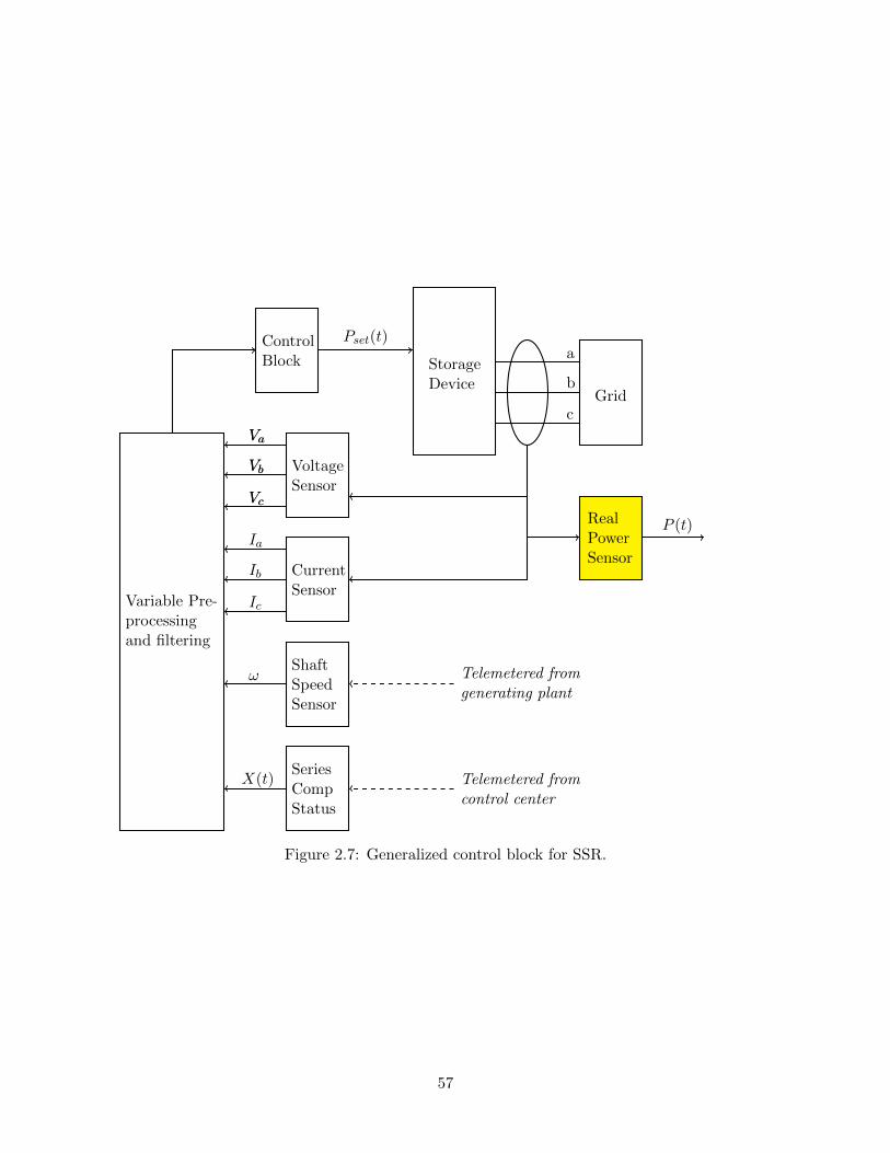
Variable Pre-processingand filtering
ControlBlock Storage
DeviceGrid
RealPowerSensor
VoltageSensor
CurrentSensor
ShaftSpeedSensor
SeriesCompStatus
a
b
c
P (t)
Pset(t)
Telemetered fromgenerating plant
Telemetered fromcontrol center
Va
Vb
Vc
Ia
Ib
Ic
Va
Vb
Vc
ω
X(t)
Figure 2.7: Generalized control block for SSR.
57

contingencies. They can only be used in circumstances where the system is in grave danger ofcollapse and extraordinary efforts are required to stabilize the situation.
UFLS relays normally trip an entire distribution feeder. They are most often set to actuatewhen system frequency drops to an unusually low value, for example 59.1 Hz in some parts of NorthAmerica. A UFLS scheme is expected to drop a known amount of load measured in MW. If anenergy storage device were present on the feeder, or in close proximity, it could inject the sameMW of real power which would net the same result as if the feeder were tripped by UFLS. In otherwords, a storage device could replace the UFLS scheme.
Similarly, if the most appropriate response to an under-voltage event is to shed load then astorage device could offset the amount of load that would normally be shed with an UVLS scheme.It must be noted that a storage device can also provide reactive power (see Section 2.5.2). In casesof extreme under-voltage, it may be more appropriate to utilize the full capacity of the storagedevice to provide reactive power rather than using the device to inject real power to offset anUVLS scheme. In other words, the voltage control benefit and the UVLS benefit may be mutuallyexclusive.
The technical requirements for storage devices participating in UFLS and/or UVLS becomesomewhat ambiguous. Once initiated, traditional UFLS and UVLS operate extremely fast, forexample 5-10 cycles or 1/6 of a second. However, the speed with which traditional UF(V)LSschemes operate is more an artifact of the speed of the circuit breaker rather than being derivedfrom basic principles. In either UFLS or UVLS the physics of the phenomenon being manipulatedis not so dependent upon speed. A rise time for the storage device on the order of 0.5 secondsshould be sufficient for the intended purpose.
Testing for UF(V)LS response would involve triggering the shed command at a variety of op-erating and state of charge conditions. At minimum, one would need to monitor the set point realpower, the actual real power being delivered (consumed) by the storage device, the actual frequencyor voltage, and the trigger frequency or voltage. The storage device should get credit for the netchange in real power when responding to the trigger event.
A PMU reporting at 60 samples per second, a sequence of events recorder, and/or a dynamicsystem monitor should be sufficient for the purpose of assessing the performance of a storagedevice claiming a UFLS/UVLS benefit. Data acquisition at reporting rates of 30 samples persecond would provide marginally adequate information. Rates of less than 30 samples per secondwould be unacceptable. Data can be stored using triggered capture provided there is a buffer ofpre-trigger data available in the recording device. Data need not be continuously recorded.
2.6 Quality and Reliability
Quality and reliability, for purposes of assessing monitoring needs, is a separate phenomenon fromregional, or bulk grid, reliability as discussed in Section 2.5. Quality and reliability addresses anytype of disturbance that may affect the ultimate end use, including poor power quality as well asfeeder and branch circuit outages. High speed data acquisition is required to assess the benefitsof storage with respect to end-use reliability. The data acquisition systems need not continuouslycollect data, but can be allowed to burst-record data sets when power quality problems are detected.The data acquisition system should be programmed to buffer an adequate amount of data prior tothe disturbance for proper analysis.
Power quality generally refers to sags, surges, harmonics and other flaws in an otherwise purelysinusoidal voltage or current. Power is still available to the process, but the power is of such poorquality as to be unusable. Reliability, on the premises of the end user, refers to the provision of
58

backup power during periods of time when power from the grid is unavailable. A reliable powersource on a premise is commonly referred to as an uninterruptible power supply (UPS).
The benefit attributable to reliable power accrues, in part, to the value of the process preservedby providing reliable power during periods of time when grid power is not available or is of poorquality. Therefore, knowledge of the underlying process is important for assessment of the benefit.In terms of physical quantities, it is critical to retrieve point-on-wave data at a high sample rate toassess power quality or reliability.
2.6.1 UPS Applications
PQ monitoring equipment is appropriate for validating the benefits of a storage device claimingUPS capability. It is prudent to keep a continuous buffer of data and to only archive the data todisk if a reliability event is detected, that is to say if the voltage of the grid connection is degraded.The triggers should be set to capture point-on-wave data when the absolute value of grid voltageexceeds a threshold value.
An uninterruptible power supply (UPS) is a storage device intended to maintain a reliable supplyof electrical energy to a critical end use. IEEE Standard 1366 defines two common metrics, SystemAverage Interruption Frequency Index (SAIFI) and System Average Interruption Duration Index(SAIDI), used to measure reliability at the customer’s meter. While SAIFI and SAIDI can varysignificantly depending upon the geographic location of the utility and the utility’s maintenancepractices, the average customer might experience slightly more than one outage per year withan average total outage time of 1.5 hours (see, for example, Exelon Corp. Annual Report athttp://www.exeloncorp.com/performance/investors/secfilings.aspx).
It is often the case that the critical load can be supplied by some fossil-based generator, forexample a diesel backup generator, for outages that last more than a few tens-of-seconds. Thereforethe performance requirements for an energy storage device intended to provide a UPS benefit isthat the storage device seamlessly “picks up” the critical load for as long as it takes for either theutility to restore normal power or for the backup generation to safely come online and to pick upthe critical load. The amount of energy capable of being delivered by the storage device must besufficient to meet the demand of the critical load until either of the above conditions occurs. Thespeed with which the storage device responds must be commensurate with the ability of the criticalload to tolerate outages.
For technical performance validation, it is not strictly necessary to record the power from thestorage device. It is assumed that if voltage to the critical load remains within the tolerance ofthe equipment supplied then the storage device is delivering acceptable reliability. A high-levelperspective for validating the delivery of this benefit is shown in Figure 2.8. Variables include:
• t = time.
• Va, Vb, Vc = the a-phase, b-phase, and c-phase point-on-wave voltages at time t.
• SoC = the state of charge of the storage device at time t.
• abc = three-phase electrical connection to grid.
2.6.2 Harmonics
The IEEE Standard 519, along with IEEE Standard 1366 and other US and international standards,define power quality in terms of the usability of electrical energy. Harmonics represent one aspectof usability. Harmonics in a power system are strictly defined as energy in frequency bands that
59
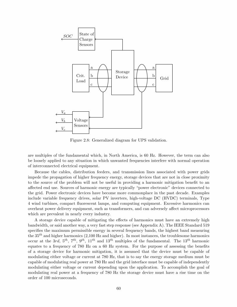
State ofChargeSensors
Crit.Load
VoltageSensors
StorageDevice Grid
Va
Vb
Vc
a
b
c
a
b
c
SOC
Figure 2.8: Generalized diagram for UPS validation.
are multiples of the fundamental which, in North America, is 60 Hz. However, the term can alsobe loosely applied to any situation in which unwanted frequencies interfere with normal operationof interconnected electrical equipment.
Because the cables, distribution feeders, and transmission lines associated with power gridsimpede the propagation of higher frequency energy, storage devices that are not in close proximityto the source of the problem will not be useful in providing a harmonic mitigation benefit to anaffected end use. Sources of harmonic energy are typically “power electronic” devices connected tothe grid. Power electronic devices have become more commonplace in the past decade. Examplesinclude variable frequency drives, solar PV inverters, high-voltage DC (HVDC) terminals, Type4 wind turbines, compact fluorescent lamps, and computing equipment. Excessive harmonics canoverheat power delivery equipment, such as transformers, and can adversely affect microprocessorswhich are prevalent in nearly every industry.
A storage device capable of mitigating the effects of harmonics must have an extremely highbandwidth, or said another way, a very fast step response (see Appendix A). The IEEE Standard 519specifies the maximum permissible energy in several frequency bands, the highest band measuringthe 35th and higher harmonics (2,100 Hz and higher). In most instances, the troublesome harmonicsoccur at the 3rd, 5th, 7th, 9th, 11th and 13th multiples of the fundamental. The 13th harmonicequates to a frequency of 780 Hz on a 60 Hz system. For the purpose of assessing the benefitsof a storage device for harmonic mitigation, it is assumed that the device must be capable ofmodulating either voltage or current at 780 Hz, that is to say the energy storage medium must becapable of modulating real power at 780 Hz and the grid interface must be capable of independentlymodulating either voltage or current depending upon the application. To accomplish the goal ofmodulating real power at a frequency of 780 Hz the storage device must have a rise time on theorder of 100 microseconds.
60

To measure the effectiveness or performance of a storage device in mitigating issues associatedwith harmonics, only a PQ monitor or custom data acquisition device capable of sampling at 5000samples per second or faster will suffice. The most straightforward method for determining theeffectiveness of the device is to perform a test wherein the voltage and current harmonics can bemeasured in a test environment, or with the device in situ, both with the storage device in serviceand with the storage device out of service. After a device is placed in service it is not adequateto simply measure the amount of energy delivered by the device at harmonic frequencies to judgethe device’s effectiveness. The system impedance seen by the device at the harmonic frequenciesof interest must also be measured to ensure that the device is providing benefit.
The next chapter presents a framework for evaluating the economic performance of grid con-nected electrical energy storage systems.
61

62

Chapter 3
Economic Performance Analysis
3.1 Introduction
New, non-traditional means of maintaining the required instantaneous balance between electric-ity demand and supply are gaining ascendancy. The traditional perspective of maintaining thatbalance, mostly from the supply side, has given way to the perspective that both consumers andsuppliers can play important roles in maintaining this balance and simultaneously reduce the costsincurred by both parties. Electrical energy storage (EES) systems constitute one of those newmeans of balancing. While some EES technologies have been around for a very long time (e.g.,pumped hydroelectric storage), others, such as flywheels, are emerging. As with most new in-vestments, evaluating these new technologies can be challenging mostly because of increasinglythorough understanding of the physics of electric systems has identified many subtleties that mustbe considered. EES, akin to load in their charging phase, present additional considerations in theirevaluation. The policy environment has also become complex and nuanced with the simultaneousexistence of differing business models in the industry.
The potential benefits of an EES storage system stem from one of the four activities:
• Sourcing real power (discharging)
• Sinking real power (charging)
• Sourcing reactive power
• Sinking reactive power
For those unfamiliar with the terms“sourcing” and “sinking”, sourcing refers to the flow out of adevice while sinking refers to the flow into a device. None of these capabilities are unique to EES.For example, traditional generation is capable of supplying real power. Loads are capable of sinkingreal power. Capacitor banks are capable of providing reactive power. Some types of traditionalgeneration are capable of absorbing reactive power. EES systems are unique in their ability toprovide all four capabilities
A discussion of the relationship between the terms energy, power, and capacity may help toclarify the discussion in this chapter. Two critical parameters of an EES system are the rated powerand energy. Energy is defined as the capacity of a physical system to perform work. Power is definedas the rate of change in energy. These relationships are captured by the following equation.
Energy =
∫ T
0Power(t)dt (3.1)
63

EES applications may be categorized by their energy and power requirements, as shown in Table3.1.
Table 3.1: Power and Energy Criteria.
Low Energy High Energy
Low Power Example: Short term distribu-tion level energy storage (min-utes)
Example: Long term distribu-tion level energy storage (e.g.days).
High Power Example: damping inter-areaoscillations. Output can be10’s to 100’s of MW, zero netenergy.
Example: large pumped hydrofacility capable of supplying100’s of MW for 8-12 hours.
Since energy is the integral of power over time, the difference between many low energy andhigh energy applications is simply time. For example, wind ramp rate limiting for a small windfarm could be classified as low power and low energy. Wind firming for the same wind farm couldbe considered low power, high energy if the EES system is required to replace lost wind generationfor long periods of time (e.g. several days). There are no firm guidelines for energy and powerthresholds. Often, they are technology dependent. A 50 MWh pumped hydro system might beconsidered “low energy” relative to other pumped hydro systems. A 50 MWh lithium batterysystem might be considered “high energy” relative to other lithium battery systems.
Other new, non-traditional means of supply and demand balancing with similarities to EESinclude “demand response” (DR), “energy efficiency” (EE), and “distributed generation” (DG).Demand response is the willingness of consumers to reduce their electricity consumption duringtimes of peak consumption, often shifting it to off-peak times. Energy efficiency refers to im-provements in electric consuming devices to reduce their electric consumption while maintaining orimproving output performance. Distributed generation is the practice of geographically dispersingsmaller generation units around the load center as compared to the large, central station generationplant.
For various reasons these other non-traditional means are further along in their diffusionthroughout the industry. Therefore, processes have been adopted1 to standardize their evalua-tion. This is fortuitous because we can use many of the evaluation principles and methodologies inthe promotion of a standard for evaluating EES technologies [18, 19, 20].
3.2 Sequential Analysis Process
A methodology for assessing investment cost-effectiveness that can compare new, non-conventionalsolutions with conventional solutions is necessary to produce technically defensible analyses thathighlight comparative costs. A four-step process for down-selecting a set of technological andpossibly non-technological solutions is recommended.
Step 1 Identify required services and solution concepts.
Step 2 Identify feasible Functional Uses (see Table 3.2).
Step 3 Identify and asses grid impacts including incidental benefits.
Step 4 Develop energy storage business cases.
1Or they are in the process of adoption.
64
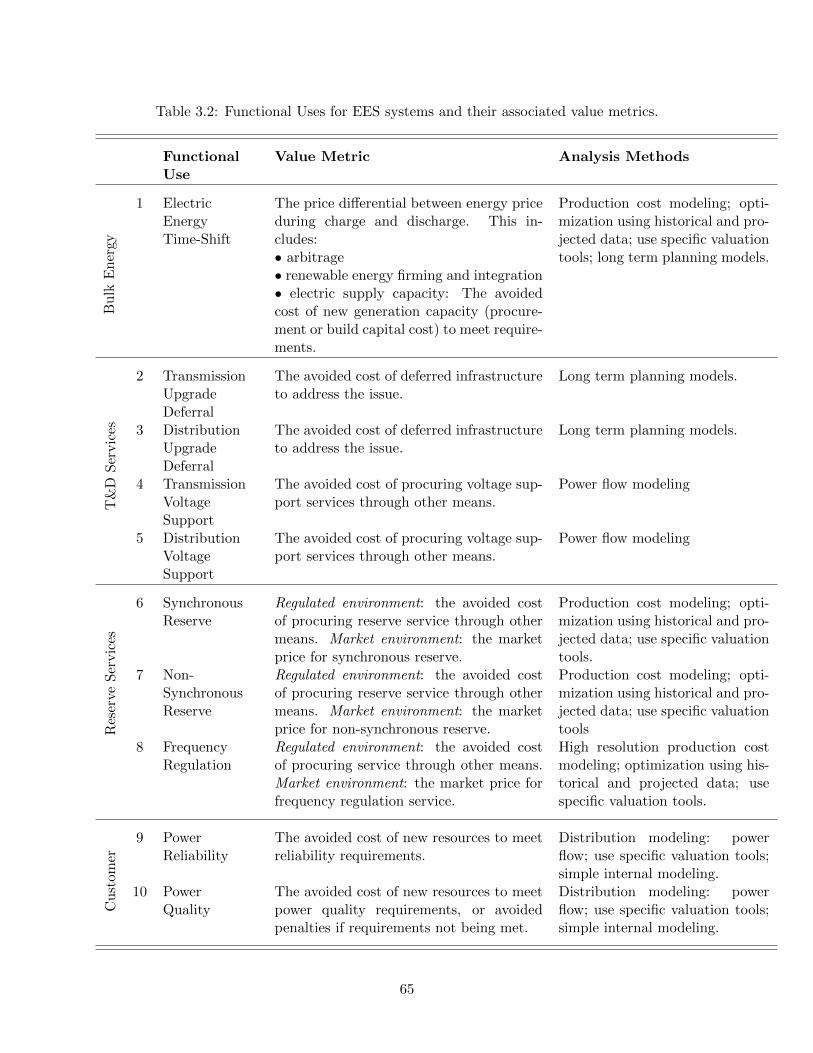
Table 3.2: Functional Uses for EES systems and their associated value metrics.
FunctionalUse
Value Metric Analysis Methods
Bu
lkE
ner
gy
1 ElectricEnergyTime-Shift
The price differential between energy priceduring charge and discharge. This in-cludes:• arbitrage• renewable energy firming and integration• electric supply capacity: The avoidedcost of new generation capacity (procure-ment or build capital cost) to meet require-ments.
Production cost modeling; opti-mization using historical and pro-jected data; use specific valuationtools; long term planning models.
2 TransmissionUpgradeDeferral
The avoided cost of deferred infrastructureto address the issue.
Long term planning models.
T&
DS
ervic
es 3 DistributionUpgradeDeferral
The avoided cost of deferred infrastructureto address the issue.
Long term planning models.
4 TransmissionVoltageSupport
The avoided cost of procuring voltage sup-port services through other means.
Power flow modeling
5 DistributionVoltageSupport
The avoided cost of procuring voltage sup-port services through other means.
Power flow modeling
Res
erve
Ser
vic
es
6 SynchronousReserve
Regulated environment: the avoided costof procuring reserve service through othermeans. Market environment: the marketprice for synchronous reserve.
Production cost modeling; opti-mization using historical and pro-jected data; use specific valuationtools.
7 Non-SynchronousReserve
Regulated environment: the avoided costof procuring reserve service through othermeans. Market environment: the marketprice for non-synchronous reserve.
Production cost modeling; opti-mization using historical and pro-jected data; use specific valuationtools
8 FrequencyRegulation
Regulated environment: the avoided costof procuring service through other means.Market environment: the market price forfrequency regulation service.
High resolution production costmodeling; optimization using his-torical and projected data; usespecific valuation tools.
Cu
stom
er
9 PowerReliability
The avoided cost of new resources to meetreliability requirements.
Distribution modeling: powerflow; use specific valuation tools;simple internal modeling.
10 PowerQuality
The avoided cost of new resources to meetpower quality requirements, or avoidedpenalties if requirements not being met.
Distribution modeling: powerflow; use specific valuation tools;simple internal modeling.
65

3.2.1 Step 1: Required Grid Services Addressed by Solution Concepts
Develop a list of required grid services, identify specifications, and define characteristics of thepotential solutions. The solutions may include EES as well as other types of technological or non-technological sources. EES may have advantages that conventional solutions lack including very fastresponse and ramp times as well as the ability to operate at non-unity power factor. The possiblyunique advantages of EES have the potential to solve problems on the grid in different contexts;other solutions may have a different set of advantages. The first step of the investigation is to askthe questions: “What is the grid operational or planning problem?” and “What technological ornon-technological solutions are available?”
After identifying a needed grid service the technical requirements can be communicated toactual stakeholders and decision-makers to determine the metrics being considered, the minimumsolution criteria, and the alternative solution(s) to the problem. The technical criteria for an energysolution can then be determined based on the site-specific information available. The value of theenergy storage solution can be determined based on the avoided cost or expected revenue of thechosen grid service. The term grid service refers to a defined need for power or energy to solve agrid issue and contains two critical elements:
1. Technical objectives and minimum requirements
2. Calculable value
3.2.2 Step 2: Identifying Feasible Functional Use Cases
A functional use case is a technically feasible combination of grid services. Each functional usecase should have an “anchor” service that drives the incentive for a grid solution; this could bea distribution investment deferral that uses a technology or other grid adjustment to delay oreliminate an expensive transformer or line upgrade.
After grid service requirements have been determined for the anchor service, the relative valueof the anchor service should be investigated to determine whether it could potentially support acost-effective use case. Depending on the size of the upgrade investment, the load characteristics(e.g. frequency and duration of peaks), and available technology or operational options this couldbe a promising anchor service. Tools are available for investigating the anchor service. A toolwould need the capability to run a time-series simulation and cost-benefit calculation for the anchorservice based on the grid service requirements and underlying site-specific data that the user canprovide2. Other grid services that are compatible technologically with the anchor service can thenbe investigated.
3.2.3 Step 3: Monetary and Non-monetary Benefits
The purpose of this step is to determine how different solution options affect the key system-widemetrics listed below:
1. Monetary benefits/costs - energy and ancillary services prices
2. Non-monetary benefits/costs
(a) Asset utilization and generator operation
2Sandia/Kema-DNV’s ES Select is an internet tool available to perform “down select” analyses at a high leveland the EPRI ESVT3.0 tool has simulation capabilities that can perform some of the required operations
66

(b) T&D losses
(c) Environmental impacts (e.g. GHG emissions)
Benefits may be monetary in that they affect prices for energy and ancillary services. They mayalso be nonmonetary if the solution option affects other asset utilization, changes T&D losses, orhas an effect on environmental metrics. Incidental benefits need not be unintended but if the benefitcannot be modeled as a grid service it does not drive the energy storage dispatch and therefore isincidental to the operation of the investment alternative under consideration. Incidental benefitsmay result from a combination of the asset dispatch and other characteristics of the electric systemleading to the observation that incidental benefits could be costs.
The steps in the process involve:
1. Assess a baseline scenario with no additional energy storage—the “no action alternative”;
2. Define and simulate likely grid deployment scenarios for alternative investments, informed byuse case cost-effectiveness;
3. Tabulate the monetary and nonmonetary benefits and costs of interest in each scenario.At the end of this process, the incidental benefits and costs of storage deployment will bequantifiable.
Particularly in a regulated environment nonmonetary benefits and costs may be relevant tohighlight differences between solution options. These are often referred to as “externalities” byeconomists. This means the benefits and costs have no opportunity to be reflected in prices atwhich resources are traded. These externalities, such as changes to asset utilization or changes totransmission or distribution losses as itemized above, can occur within the electric system underevaluation. If any of the alternatives under evaluation have these kinds of effects, they should beidentified and quantified as much as possible. So, for example, if an alternative allows greater assetutilization of other assets on the system the increase in capacity factor or other utilization measurecan be identified. Transmission and distribution losses can be handled similarly. It is possiblethat changes in capacity factors could be transformed into dollar values with particular detailedanalysis. This is also true for changes to transmission and distribution losses.
Externalities that occur outside the electric system are more than likely to be environmental orother types of externalities that affect the public at large. Guidance is somewhat similar in thesesituations in that the externalities should be identified and quantified to the extent feasible—tonsof CO2 reduction for example. Using guidelines promulgated by the federal government such exter-nalities can then be converted to monetary units based on widely accepted and vetted parameters.For example, the report of the Interagency Working Group on Social cost of Carbon, United StatesGovernment can be used to apply monetary values to carbon dioxide [21].
3.2.4 Step 4: Investment Business Cases
The final step of assessing the cost-effectiveness of alternatives is to evaluate the technology andnon-technology alternatives for functional use cases. This stage involves the organization of dataand information to conduct financial and accounting analyses. It may also involve the introductionof policy and regulation considerations that might be taken into consideration in a broader decisionmaking process that goes beyond the strict financial and economic analysis presented in businesscases3. This involves assembling data into a form in which it can be manipulated to produce the
3The EPRI ESVT3.0 is a project financial analysis tool energy geared toward EES evaluation and is capableof supporting business case simulation. It includes the capability to run discounted cash-flow and utility revenue
67

desired investment analyses. It also involves choosing investment criterion that will be applied tochoose the best alternative investment. This process is the subject of the next section.
3.3 Fundamental Evaluation Principles and Methods
Investment analysis is about choosing among alternatives. There are always alternatives available.Even in the de minimis case, the “no action” alternative, is always an option. Complications arisefrom the fact that investment alternatives may be quite different in their scale, the time distributionof benefits and/or costs, the level of risk, and in a variety of other possible ways. The analysis isfurther complicated by the fact that different types of organizations may find that certain methodsare more amenable to circumstances they find important while other types of organizations mayprefer yet another approach.
Several different approaches could be used to evaluate the cost effectiveness of EES and alterna-tive investments. Among the alternatives for organizing the information and data are the businesscase approach and integrated resource planning. Except for relatively large investments in EESsystems neither of these approaches is likely to be sufficiently fine-grained to properly measure thebenefits and costs of EES investments that are likely to have smaller impacts on a system. Analternative means to evaluate smaller investments having smaller impacts is to employ a methodbased on avoided (marginal) costs.
The “avoided cost” principle was first propounded in the Public Utility Regulatory Policy Actof 1978 as the appropriate criterion for use in evaluating competing technologies. The FederalEnergy Regulatory Commission defined that principle as the “incremental capacity and energycost a utility would have incurred if they had built their own capacity rather than purchase energyfrom a qualifying facility.” While there was controversy over how that principle was applied insome cases it remains appropriate for evaluation of EES technologies [22].
This principle derives from the economic concept of opportunity cost, which holds that thevalue resulting from undertaking action “A” is equivalent to avoiding cost by not undertaking “B”.As is evident from the above statement the terms avoided cost and opportunity cost are relativeand have meaning only in reference to some base action or condition. The principle is effective onlyin comparing alternative courses of action.
3.4 Evaluation Perspectives
One important fact to keep in mind in evaluating any investment in the electric utility industry isthe business model that pertains to the particular geographic area in which the investment is to belocated. Generally one can distinguish between the “state-regulated, vertically integrated utility”business model and “market resource allocation areas”. This is important because evaluations mayneed to be structured somewhat differently depending upon the business model existing in the areaof interest.
Vertically integrated utilities’ investment evaluations turn on cost differentials between twoor more alternatives since the business objective of the entity is likely to be some variant of costminimization together with the requirement to serve load. Such an entity could also perform revenuerequirements analyses to demonstrate the impact of the investment on electric rates. This approachalso resonates with regulators whose constituents’ interests are served by keeping electricity prices as
requirement analyses, and can generate financial proforma statements including debt, equity, and tax assumptions.Policy scenarios, such as simulating the effect of an investment tax credit, can be run easily by adjusting financialand economic assumptions.
68

low as possible. If the utility commission approves the investment request, the utility is permitted toadd the value of the investment to the “rate base” (base on which the utility may earn its allowedrate of return) and return of invested funds over the life of the investment is then somewhatguaranteed. This may mean that the evaluation needs to consider a longer list of alternatives todemonstrate least cost. It could also be that the utility commission requests information on thenon-market benefits of the proposed investment as well. It is likely that the decision to move forwardwith the investment will turn on a combination of considerations beyond the narrow profitabilityof the investment. Utility commission approval is normally sufficient to obtain debt funding fromcapital markets.
An independent third-party investor, such as an independent power producer (IPP), mightpropose an investment in a specific regulated utility’s service territory. In such a case, three inde-pendent but related types of analyses might be performed: analyses examining the profitability ofthe investment to the developing entity, analyses that the investor would use to convince the utilityof the merits of the investment, and analyses that would help the utility convince its regulatorycommission on the merits of the investment.
In contrast, entities doing business in areas characterized by wholesale market resource alloca-tion are in competition with each other to supply the market demand for electricity. They offertheir resource into forward auction-type markets at specified offer prices. If their offers are accepted(cleared in the market) they will supply a portion of the market demand. If their offer price is toohigh they will not be cleared and cannot supply the market. Unless such entities are operatingunder a Power Purchase Agreement or a Tolling Agreement, they operate on the potential for profitbut have no backstop guarantee that they will be profitable. Investment evaluation for this type ofentity follows a more standard “business case” approach. Evaluation in this circumstance is likelyto be narrower in that the firm will already be in possession of a technology and will want to de-termine whether a profit can be made in the application of that technology to provide a particularservice.
In the evaluation approaches set out below, we make an effort to consider the effect of thebusiness model and the organizational nature of the entity making the proposal on the type ofanalyses that are likely to be performed and on the criteria used to make decisions on the investment.
State-regulated, Vertically Integrated Utility (VIU) Business Model
This is the traditional regulated utility business model that originated in the early decades ofthe 20th Century and remains in use in the southeastern and western regions of the U.S. It consistsof organizational entities that functionally bundle generation, transmission, and distribution intoone organization. Such organizations are usually privately owned but their operations are subject topublic utility commission oversight. They must obtain approval from their regulatory commissionfor new capacity investment and changes in the “rates” (prices) charged to their customers.
Market Resource Allocation Business Model
These areas are characterized by unbundled generation and more open access to organized whole-sale markets by non-traditional entities (Independent power producers, merchant plants, etc.).Theyare subject to Federal Energy Regulatory Commission (FERC) regulation of market rules and pro-tocols and to interstate commerce of electricity when it enters the transmission network. Formerlyvertically integrated utilities that have divested generation and serve the final consumer in the roleof “load serving entities” (LSE) supply consumers at rates regulated by state regulatory commis-sions. Given this regulatory structure the cumbersome phrase “market resource allocation” areas
69

is used to distinguish this business model from the state-regulated, vertically integrated utilitybusiness model.
3.5 Evaluating EES Functional Uses
Step 2 of the evaluation process described above recommended identifying functional use cases tobe evaluated. Table 3.2 includes a list of Functional Uses that EES technologies can provide at gridscale along with the metrics that should be used in the evaluation of a device in a specific locationproviding the identified Functional Uses.
3.6 Effect of Organization Type on Investment Analysis
Entities proposing to invest in EES are most likely to be privately owned firms whose sharesare publicly traded or at least traded OTC; they may be IPPs, merchant plants, VIUs or anyof a variety of other business entities. As private sector entities, they need to pay particularattention to the effect of their decisions on shareholder or investor value. They can do this byensuring investment opportunities meet their internal decision criteria before proceeding. Theymay examine investments as to their rate of return on investment, rate of return on equity, internalrate of return, discounted cash flow, short-term and longer-term cash flow projections, and otherinvestment criteria they may choose to apply.
After determining that proposed investments meet their criteria and are in the interests ofthe entity, they may then perform other investment analyses which support advancement of theproposal. At this juncture the comparison of a specific technology alternative to other possiblealternatives could be necessary or desirable. In the case of the VIU, it may be necessary in makingthe case before the regulatory commission that this particular technology is the lowest cost alter-native to solve the problem. In the case of an IPP, it may be necessary to demonstrate to a utilityfrom which the IPP is seeking a power purchase agreement (PPA) that this is the best alternativesource of energy. Whatever the particular circumstances of the case are, analysis of alternativesolutions is required.
3.7 Which Type of Investment Analysis?
Investment criteria are used for making decisions in regard to specific investments. A number ofcriteria are available and have typically been used for accepting or rejecting specific investmentsor ranking investments for various purposes. Table 3.3 identifies the most commonly used criteria,and provides a brief description of each together with the units in which the criterion is expressed.The most commonly used of the ten criteria listed in Table 3.3 are NPV, B/C, and LCOE.
70

Table 3.3: Typical Investment Criteria [6].
InvestmentCriterion
Typical Acronym Brief Description Units
Net PresentValue
NPV Discounted sum of future benefits mi-nus costs
Present ValueDollars
Total LifeCycle Costs
TLCC Sum of future costs over project life Dollars
RevenueRequirements
RR Future revenue required to offset allcost (regulated environment)
Dollars
Levelized Costof Energy
LCOE Annuitized cost per energy unit Dollars/EnergyUnit
Internal Rateof Return
IRR Rate of return that equalizes presentvalue of receipts and expenditures
Percentage
ModifiedInternal Rateof Return
MIRR Same as IRR except regarding rein-vestment at discount rate
Percentage
SimplePayback
SPB Number of years to accumulate rev-enues equal to investment outlays
Years
DiscountedPayback
DPB Same as SPB except revenues & in-vestment outlays are discounted
Years
Benefit-costratio
B/C Discounted total benefits divided bydiscounted total costs
Fraction,decimal
Savings toInvestmentRatio
SIR Modified B/C ratio where principalinvestment costs are in denominatorand all other costs are subtracted frombenefits in numerator
Fraction,decimal
71

For internal analyses, such as described above, firms will likely restrict their models to theconsideration of actual monetary cash flows—future streams of revenues and costs. In regulatedenvironments where revenues are fairly fixed (“sticky” regulated rates), decisions will likely turnon the difference in costs between different technologies. In market resource allocation areas, therevenue streams will result from offering assets into auction markets. Discounted cash flow will bea main analysis methodology and net present value (NPV) will be the investment criterion. Anyproject with a positive NPV merits further consideration.
Other investment criteria are in common use and there is really no absolute guideline as towhich is the most appropriate, particularly when considering all possible circumstances. NPVprobably comes closest to this ideal. While NPV is perhaps the most commonly used criterion,particularly in private sector firms, levelized cost of energy (LCOE) is also widely used, particularlyin regulated environments. Fortunately, the question of which investment analysis approach andwhich investment criterion is most appropriate has been reported in the literature. Table 3.4 is anexample and is adapted from a lengthier table appearing in [6].
Table 3.4: Guideline Suggestions for Investment Criteria Applicability [6].
Investment Decision NPV LCOE B/C IRR RR
Accept or reject A,C A,C A,C A,C NR
Select from mutually exclusive alternatives R NR NR NR A
Ranking A A NR NR A
Legend: A: Acceptable, C: Common, NR: Not Recommended.
Other key insights and recommendations from [6] include:
• Levelized cost of energy, internal rate of return, modified internal rate of return, simplepayback period, discounted payback period, benefit-cost ratio, savings-to-investment ratioare not recommended for analysis of mutually exclusive alternatives because these measuresdo not normalize for the scale of different investment alternatives.
• Revenue requirements (RR) analysis is recommended for investments in a regulated environ-ment. (It is noted that RR analysis is generally required for any regulated utility to submit toits commission. However, in internal decisions, the utility will likely employ other analysesand measures to assure its executives and board that a given investment is in the best interestof the organization.)
• Only NPV is recommended as an investment criterion for decisions on mutually exclusiveprojects. Incremental B/C analysis is equivalent to maximizing the NPV (See Appendix B).
3.7.1 Discounted Cash Flow/Net Present Value
A simple generalized formula for calculating discounted cash flow is given by:
DCF =N∑i=1
Ri − Ci(1 + r)i
(3.2)
72

where
DCF discounted cash flow (net present value)Ri, Ci revenue and cost in period ir discount rate, interest rateN number of periods
This is a straightforward type of analysis that is performed in many areas of business includinginvestments of real capital as well as financial investments.
3.7.2 Calculating Levelized Cost of Electric Energy
Levelized cost of energy (LCOE) is the cost per unit of energy produced (or saved) by the systemover the analysis period that will sum to the total life cycle cost when discounted back to the baseyear. It is used to compare alternative investments even if they have different scales of operation,different investment, and/or operating periods. A generalized formula for LCOE is [6]
LCOE =
N∑i=1
Ci(1 + r)i
N∑i=1
Qi(1 + r)i
(3.3)
where
LCOE levelized cost of energyCi cost associated with period iQi energy output or energy saved in time period ir discount rate, interest rateN number of periods
Total life cycle cost (TLCC) is calculated as follows:
TLCC =N∑i=1
Ci(1 + r)i
(3.4)
The costs in any time period include investment costs, finance charges, potential salvage value,non-fuel operations and maintenance costs, replacement costs, and fuel costs.
3.7.3 Relationship between DCF/NPV and LCOE
There is a clear relationship between these two investment criteria. When the incremental revenuesare zero or are unchanged across a number of different technologies, then the alternative technologiescan be compared based on the NPV of their costs4. Levelizing a stream of benefits or costs (ortheir net amount) is a process in which (i) the NPV is calculated using the stream of future receiptsand or payments; and (ii) calculating the equal annual payment whose present value equals theoriginal NPV. Therefore, the investment criteria NPV and LCOE are equivalent. The convenienceof LCOE is that its units are in terms of dollars per unit of energy (e.g., $/kWh) which allowsdirect comparison between projects of different scale or technology. In contrast, PV or NPV is inunits of money but they’re not the units of money with which we’re familiar—they’re not nominaldollars.
4See Appendix B of this report.
73

3.7.4 Effect of Nonmonetary Costs and Benefits
The literature describing the potential benefits of EES devices emphasizes the nonmonetary, in-cidental benefits that may be conferred by investments in these devices. In fact, most of theother technologies that compete with EES devices to provide Functional Uses will similarly providenonmonetary benefits. There may be differential amounts of incidental benefits provided or costsincurred by the alternatives so this needs to be carefully evaluated for each option. For example,a combustion turbine will likely provide some incremental incidental benefits of GHG emissionscompared with a coal plant but the turbine will not provide as large a benefit stream as a largebattery EES system.
3.8 Functional Use Evaluation Approaches
This section sketches the process and key features of an evaluation of each of the Functional Useslisted in Table 3.2.
3.8.1 Electric Energy Time Shift
This functional use is accessible only to EES systems; systems that have the capability to chargethe storage device when off-peak energy price is relatively low and discharge the stored energy whenenergy price is relatively high, earning the differential to contribute to capital and O&M for thesystem. In an unregulated environment this produces a net revenue stream for the asset owner.In a regulated environment the utility can potentially reduce cost of transmission congestion byengaging in energy time shift. When energy demand is peaking, it is necessary to utilize eventhe most expensive generators in the utility’s fleet. EES could potentially be substituted for moreexpensive generators and reduce the utility’s cost of operation.
Key Variables/Parameters Required for Evaluation in Regulated areaThe following items should be used in the evaluation:
• Levelized annual capital cost of EES technology $/kw
◦ Technology specific assumptions such as useful life, number of cycles per year, periodicreplacements (such as for batteries), depth of discharge, etc.
◦ Charge/discharge efficiency of EES device
− Can be handled by estimation of charge versus discharge hours during year
• Levelized annual cost of O&M of EES technology $/kwh-yr
◦ Requires forecasting hours of actual operation per year—capacity factor
◦ May necessitate an optimization or repeated simulation to determine the number ofhours of operation at which cost is minimized
• Financing assumptions
◦ Debt/equity ratio
◦ Cost of capital
• Other assumptions regarding financial, accounting, and economic variables
◦ Depreciation assumptions
74

◦ Tax credit programs
◦ Income tax assumptions
• Credits for reduction in transmission congestion—nonmonetary incidental benefits
It is assumed that this information will be available for each of the Functional Uses. It will notbe repeated for each one.
Key Variables/Parameters for Evaluation in Market Resource Allocation Area
• Estimated revenues from sales of energy at peak prices ($/kwh)
• Estimated costs from purchases of energy at off-peak prices ($/kwh)
• Annual net revenue (revenue minus cost) that could be earned from electricity sales into ASmarkets and/or other services that are compatible with use of the resource for energy timeshifting ($/kwh)
• Credits for reduction in transmission congestion FTRs
Organizing the Investment Decision
VIU Business Model
EES systems are the only supply side technology with the capability to move energy throughtime—the equivalent of peak shaving. The only other alternative that is comparable to EES inthis functional use is demand response. Accordingly, the alternatives to be evaluated are the EESsystem and a program to shift demand from peak to off-peak times. The benefit of reducing peakdemand for the VIU is reduction in the cost of operating the most expensive generators in the fleet.Since this benefit would be the same for both alternatives, a direct comparison of the LCOE of theEES system and the LCOE of a demand response program could be made.
Market Resource Allocation Model
For an unregulated firm the decision to invest in an EES system with the capability to shiftenergy in time is governed by the excess of annual net revenue (revenue minus cost) from the sale ofelectricity over the annual levelized cost of energy calculated for the particular EES system beingevaluated.
3.8.2 Transmission Upgrade Deferral
The benefit to be achieved by deferring an investment to upgrade transmission is the avoidedfinancing and other equity cost of the upgrade for the duration of its deferral. The question to poseis “Will the upgrade deferral be temporary or permanent?” The proper evaluation methodologydepends upon the intent of the deferral. If the deferral is temporary, the proper approach is tocompare the time stream of benefits and costs of the project installed immediately versus the timestream of benefits and costs with the project delayed for a specific period of time. In this case,the evaluation would be of these two project timing alternatives with a third alternative whichincorporates the means of achieving the delay. Presumably this would include some form of EEStechnology, conventional technology, or a non-technology solution.
75

Organizing the Investment Decision
VIU Business Model
This approach would compare the incremental cost obtained from subtracting the cost of thedeferred and un-deferred options to the LCOE of the third alternative. If the deferred upgrade isviewed as a permanent solution then the avoided cost is the entire value of the project that waspermanently deferred. It is assumed that the third “next best” alternative to EES is a combustionturbine. Thus a combustion turbine could be the “benchmark” or “base case” alternative and itsLCOE would be evaluated using the LCOE calculator. EES and other alternatives would then becompared on the same LCOE basis.
Market Resource Allocation Model
In a market setting the industry is functionally unbundled with the transmission network ownedby different entities than those that operate it. In this environment, it is unclear how an entitywould organize an effort to substitute some other resource or technology for a transmission upgrade.Different models and approaches are identified and discussed in the literature. With the exceptionof ERCOT, no general solutions have been achieved [23, 24].
3.8.3 Distribution Upgrade Deferral
The benefit achieved by deferring an investment to upgrade distribution is the avoided financing andother equity cost of the upgrade for the duration of its deferral. The question to pose is “Will theupgrade deferral be temporary or permanent?” The proper evaluation methodology depends uponthe intent of the deferral. If the deferral is temporary, the proper approach is to compare the timestream of benefits and costs of the project installed immediately versus the time stream of benefitsand costs with the project delayed for a specific period of time. In this case, the evaluation wouldbe of these two project timing alternatives with a third alternative which incorporates the meansof achieving the delay. Presumably this would include some form of EES technology, conventionaltechnology, or a non-technology solution.
Organizing the Investment Decision
VIU Business Model
This approach compares the incremental cost obtained from subtracting the cost of the deferredand un-deferred options to the LCOE of a third alternative. If the deferred upgrade is viewed as apermanent solution, then the avoided cost is the entire value of the project that was permanentlydeferred. It is assumed that the third “next best” alternative to EES is considered to be a com-bustion turbine. Thus a combustion turbine could be the “benchmark” or “base case” alternativeand its LCOE would be evaluated using the LCOE calculator. EES and other alternatives wouldthen be compared on the same LCOE basis.
Market Resource Allocation Model
In a market setting the industry is functionally unbundled with the distribution system typicallystill owned by the regulated utility that existed before restructuring. In a few states, efforts tounbundle the retail market are under way. Given this structure, it is likely that the distributionnetwork ownership entity would treat the investment much like it would under the regulated utilitymode. This would essentially involve a “rate basing” initiative.
76

3.8.4 Voltage Support for Transmission and Distribution
These two Functional Use categories are handled similarly to Transmission and Distribution Up-grade Deferral. In fact, providing voltage support involves the same set of options as taking actionsto defer upgrades.
3.8.5 Reserves: Synchronous, Non-synchronous, Frequency Regulation, Power Reliability, PowerQuality
These four functional use categories are essentially equivalent to an option to provide power/energyas required by the application. For these Functional Uses, EES systems are likely to encounter theirstiffest competition from conventional technologies. EES systems are energy-limited compared toconventional resources. Nevertheless, they do have the advantage of extremely fast and accurateresponse times, which may be valuable to their use as reserves. Regulation reserve is the usecommonly mentioned, and energy storage is commonly employed in uninterruptible power supply(UPS) applications.
In market resource allocation areas, rules are evolving and becoming more accommodating toEES systems. Offering an EES asset in wholesale reserve markets in an unregulated environmentproduces a net revenue stream for the asset owner. In a regulated environment, the utility canpotentially reduce cost of reserve provision by using these extremely fast responding resources.How can this happen? The greater responsiveness and accuracy may result in a reduction of thetotal capacity that is held in reserve freeing up these resources to be used more economicallyelsewhere. If EES resources are not called upon to inject energy, they have the opportunity to sellstored energy as other services
Organizing the Investment Decision
VIU Business Model
In many utility jurisdictions the “next best” alternative to EES for electric supply capacity isconsidered to be a combustion turbine. As such a combustion turbine could be the “benchmark”or “base case” alternative and its LCOE would be evaluated using the LCOE calculator. EES andother alternatives would then be compared on the same LCOE basis.
Market Resource Allocation Model
The investment decision is governed by the excess of annual net revenue from sales of capacityfor reserve and/or sale of electricity into energy markets over the annual levelized cost of energy ofthe combustion turbine on the one hand and the EES system on the other.
3.9 Stacking Benefits
In order to maximize the value or revenue stream from an EES system, it is common to identifymultiple potential Functional Uses. In theory, this will increase the value of the system. Thispractice presents two challenges. First, from a valuation perspective it becomes more difficult toassign a value to the services provided and brings in the possibility of “double-counting” benefits,which will result in an inflated valuation. Second, from an operational perspective it is a challengeto identify control algorithms that provide the multiple Functional Uses while maximizing thepotential value of the system. The most straightforward approach to evaluating a scenario withstacked benefits is to rely on a state-of-charge model of the EES system to guarantee that theFunctional Uses are served without violating the physical characteristics of the system.
77

An EES model that incorporates storage efficiency and conversion efficiency is given by
St = St−1 + γcqct − qdt − γsSt−1, (MWh) (3.5)
where
St Energy stored at the end of time period tSt−1 Energy stored at the end of time period t− 1γc Conversion efficiency (percent)qct Quantity of energy pulled from the grid (charge) during time period t (MWh)qdt Quantity of energy provided to the grid (discharge) during time period t (MWh)γs Storage efficiency (percent)
Additional parameters associated with the model are the length of the time period, the maximumcharge/discharge quantities and the maximum storage capacity of the system. These quantities aredefined as:
∆t time period (for example, hours)q̄D maximum quanitity that can be sold/discharged in a single period (MWh)q̄R maximum quantity that can be bought/recharged in a single period (MWh)S̄ maximum storage capacity (MWh)
In a stacked benefit scenario, it is helpful to keep track of the amount of energy charged ordischarged during each time period for each activity. This insures that the constraints of the deviceare met at all times and the revenue can be allocated based on the service provided. It also makesit harder to double count benefits because each benefit is a function of the energy transaction. Fora scenario with N potential benefits, the charge and discharge quantities are given by
qct =N∑i=1
qct (i), (MWh) (3.6)
qdt =N∑i=1
qdt (i), (MWh) (3.7)
where qct (i) is the charging energy associated with the ith activity and qdt (i) is the discharging energyassociated with the ith activity
The revenue at each time step is given by
Rt =N∑i=1
qd(i)t(Pdt (i)− Cdt (i))−
N∑i=1
qct (i)(Pct (i) + Cct (i)) (3.8)
where
P dt (i) Price received for discharging at time period t for the ith activity ($/MWh)Cdt (i) Cost for discharging at time period t for the ith activity ($/MWh)P ct Price paid for charging at time period t for the ith activity ($/MWh)Cct Cost for charging at time period t for the ith activity ($/MWh)
The present value of the energy storage system operating for T time increments can be writtenas
Present Value =T∑t=1
(N∑i=1
qd(i)t(Pdt (i)− Cdt (i))−
N∑i=1
qct (i)(Pct (i) + Cct (i))
)e−rt (3.9)
78

Using this relationship, it is possible to calculate the present value of a system using either historicalor estimated price data under a wide range of scenarios with stacked benefits. The charge/dischargequantities can be derived to maximize revenue (e.g. a linear programming optimization problem)or are generated by a candidate control algorithm. In a market area one can utilize historical pricedata. In a vertically integrated utility, the most difficult task is estimating the appropriate pricesand costs to use in the model. An example of estimating the maximum potential revenue fromparticipating in arbitrage and frequency regulation is described in [15].
The last chapter provides a summary of the information presented in this report.
79

80

Chapter 4
Summary and Conclusions
As the amount of renewable generation increases, the inherent variability of wind and photovoltaicsystems must be addressed in order to ensure the continued safe and reliable operation of thenation’s electricity grid. Grid-scale energy storage systems are uniquely suited to address thevariability of renewable generation and to provide other valuable grid services. The goal of thisreport was to quantify the technical performance required to provide different grid benefits and tospecify the proper techniques for estimating the value of grid-scale energy storage systems.
Evaluating the technical performance of an energy storage system with respect to a well-definedset of requirements is relatively straightforward. Unfortunately, in the electric power industrystandards vary by region, and in some cases are vague or nonexistent. A good example is theperformance required to participate in the frequency regulation market. FERC order 755 statesthat providers must be “paid for performance”. Even though this is a step in the right direction,each ISO is developing their own approach for meeting FERC order 755. This regional approachresults in a system where the “value” of an energy storage system is highly location dependent.The same holds true for voltage support services. In addition to being able to provide the properreactive power levels, the device must also be located in a suitable location in the grid. Theseexamples highlight some of the difficulties in evaluating the technical and economic performance ofan energy storage system. Both depend not only on the characteristics of the device, but also on thelocation in the grid. The approach taken in this report was conservative. Technical performancespecifications were outlined that if met, then assuredly the device can claim it serves that issue.But, if the device does not meet the requirements, it could still help in the given issue dependingon the extent to which the requirements are not met.
The economic section outlined a four-step sequential analysis process for evaluating energystorage systems:
Step 1 Identify required services and solution concepts.
Step 2 Identify feasible Functional Uses.
Step 3 Identify and assess grid impacts including incidental benefits.
Step 4 Develop energy storage business cases.
A functional use is a technically feasible combination of grid services. This report defined tenFunctional Uses for an electricity energy storage system. Several different investment criteria werethen identified and guidelines were put forth for different investment decisions. The process and keyfeatures were sketched out for each of the ten Functional Uses. The report concludes with a brief
81

discussion on the valuation of stacked benefits via a state-of-charge model for the EES. One of thebenefits of this approach is that by assigning quantities of energy to each activity, the constraintsof the system are guaranteed to be met and it is more difficult to “double count” benefits, whichwould result in an inflated valuation.
82

Bibliography
[1] H. F. Campbell and R. P. C. Brown, Benefit-Cost Analysis: Financial and Economic Appraisalusing Spreadsheets. Cambridge: Cambridge University Press, 2003.
[2] J. Eto, J. Undrill, P. Mackin, R. Daschmans, B. Williams, B. Haney, R. Hunt, J. Ellis, H. Illian,C. Martinez, M. O’Malley, K. Coughlin, and K. LaCommare, “Use of frequency responsemetrics to assess the planning and operating requirements for reliable integration of variablerenewable generation,” Tech. Rep. LBNL-4142E, Ernest Orlando Lawrence Berkeley NationalLaboratory, December 2010.
[3] D. G. Newnan, T. G. Eschenbach, and J. P. Lavelle, Engineering Economic Analysis. OxfordUniversity Press, 11th ed., 2012.
[4] A. Shoucri and D. Baker, “Montana wind power variability study.”http://commerce.mt.gov/content/Energy/docs/Presentations/MontanaVariabilityStudy.pdf.GENIVAR, Calgary, AB. Report commissioned by Northwestern Energy and the MontanaDepartment of Commerce.
[5] R. Wang and D. Baker, “Alberta wind power variability study.”http://www.aeso.ca/downloads/WindVariabilityFinalReport.pdf. Phoenix Engineering,Chestermere, AB. Report commissioned by Alberta Electric System Operator.
[6] W. Short, D. J. Packey, and T. Holt, “A manual for the economic evaluation of energy efficiencyand renewable energy technologies,” Tech. Rep. NREL/TP-462-5173, National Renewable En-ergy Laboratory, Golden, CO, March 1995.
[7] North American Electric Reliability Corporation (NERC), “Glossary of terms used in reliabilitystandards, February 12, 2008.” http://www.nerc.com/files/Glossary 12Feb08.pdf.
[8] K. Ogata, Modern Control Engineering (5th Edition). Boston: Prentice Hall, 2009.
[9] B. C. Kuo, Digital Control Systems. New York: Oxford University Press, 1997.
[10] K. J. Astrom and B. Wittenmark, Computer-Controlled Systems: Theory and Design (3rd
Edition). New York: Prentice Hall, 1996.
[11] R. C. Dorf and R. H. Bishop, Modern Control Systems (12th Edition). New York: PrenticeHall, 2010.
[12] J. James and N. Weber, Interest Rate Modelling. Baffins Lane, Chichester, West Sussex PO191UD, England: John Wiley and Sons, Ltd., 2004.
83

[13] Office of Management and Budget, “Circular A-94, Appendix C, dis-count rates for cost-effectiveness, lease purchase, and related analysis.”http://www.whitehouse.gov/omb/circulars a094/a94 appx-c.
[14] C. T. Hendrickson, L. B. Lave, and H. S. Matthews, Environmental Life Cycle Assessment ofGood and Services: An Input-Output Approach. Washington, DC: RFF Press, 2006.
[15] R. Byrne and C. Silva-Monroy, “Estimating the maximum potential revenue for grid connectedelectricity storage: Arbitrage and the regulation market,” Tech. Rep. SAND2012-3863, SandiaNational Laboratories, Albuquerque, NM, December 2012.
[16] J. Eyer and G. Corey, “Energy storage for the electricity grid: Benefits and market potentialassessment guide,” Tech. Rep. SAND2010-0815, Sandia National Laboratories, Albuquerque,NM, February 2010.
[17] A. Akhil, H. Zeininger, J. Hurwitch, and J. Badin, “Battery energy storage: A preliminaryassessment of national benefits,” Tech. Rep. SAND93-3900, Sandia National Laboratories,December 1993.
[18] California Public Utilities Commission, “California energy efficiency evaluation proto-cols: Technical, methodological, and reporting requirements for evaluation professionals.”http://www.cpuc.ca.gov/puc/, April 2006.
[19] California Public Utilities Commission, “Attachment 1: 2010 cost effectiveness proposals.”http://www.cpuc.ca.gov/puc/, December 2010.
[20] California Public Utilities Commission, “Self-generation incentive program: Frame-work for assessing the cost-effectiveness of the self-generation incentive program.”http://www.cpuc.ca.gov/puc/, March 2005.
[21] Interagency Working Group on Social Cost of Carbon, United States Government, “Technicalsupport document: - social cost of carbon for regulatory impact analysis – under executive or-der 12866.” http://www.whitehouse.gov/sites/default/files/omb/inforeg/for-agencies/Social-Cost-of-Carbon-for-RIA.pdf, February 2010.
[22] The Brattle Group, “PURPA: Making the sequel better than the original.”http://www.eei.org/whatwedo/publicpolicyadvocacy/stateregulation/documents/purpa.pdf,December 2006.
[23] S. Oren, G. Gross, and F. Alvarado, “Alternative business models for transmission investmentand operation.” http://certs.lbl.gov/ntgs/issue-3.pdf.
[24] S. Fink, K. Porter, C. Mudd, and J. Rogers, “A survey of transmission cost allocation method-ologies for regional transmission organizations,” Tech. Rep. NREL/SR-5500-49880, NationalRenewable Energy Laboratory, February 2011.
84

Appendix A - Dynamic Response
Step Response
A step response of a system is the response to an instantaneous step at the input. A normalizedresponse is shown in the below figure. The input step has an amplitude of one. Key variables are:
• Tr = Rise Time = Time to rise within 90% of the final value.
• Tp = Peak Time = Time to reach the peak value of the response.
• Ts = Settling Time = Time to settle within 5% of final value.
• %OS = Percent Overshoot =
(Peak V alue− Final V alue
F inal V alue
)100
Figure A.1: Key parameters of a normalized step response.
85

Dynamic Availability
The below figure shows a “Dynamic Availability” test. An input consisting of a series of three 50%duty cycle pulse trains separated by constant values is applied to the system. The output is thenrecorded with time-stamps corresponding to the input. Parameters include:
• Amax = the max amplitude of the input.
• Amin = the min amplitude of the input.
• Amid = the starting and ending value of the input.
• Tc1 thru Tc4 = length of time to hold input constant.
• Tp1 thru Tp3 = length of time for pulsing input.
• fp =frequency of pulsing signal (Hz).
Figure A.2: Dynamic availability test.
86

Appendix B - Incremental Benefit Cost Analysisand Net Present Value Analysis
Many engineering economics texts recommend an incremental benefit-cost analysis for three ormore mutually exclusive alternatives [3]. Although most mention that this is consistent with apresent worth analysis, this is often overlooked. In this appendix we illustrate the equivalencebetween incremental benefit-cost analysis and the maximization of net present value (NPV).
The steps for performing an incremental benefit-cost analysis are outlined below [3].
1. Identify all relevant alternatives.
2. Calculate the B/C ratio of each alternative.
3. Rank order the projects from smallest to largest cost.
4. Identify the increment under consideration. The first increment is always the lowest costoption compared to the do-nothing alternative.
5. Calculate the B/C ratio for the incremental cash flows.
6. Use the incremental B/C ratio to select the most desirable option.
7. Iterate to Step 4 until all increments have been considered.
8. Select the project with the last justified increment.
In order to show that this approach is equivalent to maximizing the NPV, first consider cash flowA and B. The NPV of each cash flow is defined as
NPV (A) =
N∑i=0
Ai(1 + r)i
(B.1)
NPV (B) =
N∑i=0
Bi(1 + r)i
(B.2)
The incremental cash flow is defined as
∆Cashflow =
N∑i=0
Ai −Bi(1 + r)i
=
N∑i=0
Ai(1 + r)i
−N∑i=0
Bi(1 + r)i
= NPV (A)−NPV (B) (B.3)
Therefore, the incremental benefit or cost is simply the difference in the net present value of thebenefits or costs.
Following the incremental benefit-cost analysis steps, the different projects are rank orderedfrom smallest to largest cost.
Ranked projects =
(B1
C1,B2
C2,B3
C3, . . . ,
BNCN
), where Ci ≥ Ci−1, i = 2, 3, . . . , N (B.4)
87

When considering the incremental B/C ratio in step 6, it is always a pairwise comparison betweentwo options (renumbered a and b).
∆B
∆C=Bb −BaCb − Ca
(B.5)
if the ratio is greater than 1.0, project b is selected and project a is discarded. Likewise, if the ratiois less than or equal to 1.0, project a is selected and project b is discarded. If the incremental B/Cratio is greater than 1.0, we have the following
Bb −BaCb − Ca
> 1.0 (B.6)
Bb −Ba > Cb − Ca (B.7)
Bb − Cb > Ba − Ca (B.8)
NPV (b) > NPV (a) (B.9)
Similarly, for the case of an incremental B/C ratio less than or equal to 1.0,
Bb −BaCb − Ca
≤ 1.0 (B.10)
Bb −Ba ≤ Cb − Ca (B.11)
Bb − Cb ≤ Ba − Ca (B.12)
NPV (b) ≤ NPV (a) (B.13)
Therefore, each step of the incremental benefit-cost analysis is equivalent to selecting the projectwith the largest net present value. Applying this to the rank order pairs results in selecting theproject with the highest net present value. This shows the equivalence between incremental benefit-cost analysis and selecting the project with the highest NPV.
88

This page intentionally left blank.
89

DISTRIBUTION:
1 Dr. Imre GyukProgram Manager, Energy Storage ResearchOffice of Electricity Delivery and Energy ReliabilityU.S. Dept. of EnergyWashington, DC 20585
1 Dr. Dan TrudnowksiMontana Tech UniversityElectrical Engineering Department1300 W. Park StreetButte, MT 59701
1 Dr. Matt DonnellyMontana Tech UniversityElectrical Engineering Department1300 W. Park StreetButte, MT 59701
1 MS 1104 Robert Q. Hwang, 61101 MS 1140 Ross Guttromson, 61131 MS 1152 Steven F. Glover, 16541 MS 1033 Charles J. Hanley, 61121 MS 1152 Jason C. Neely, 16541 MS 1140 Raymon H. Byrne, 61131 MS 1140 Cesar A. Silva Monroy, 61131 MS 1140 David A. Schoenwald, 61131 MS 1140 Georgianne Huff, 61131 MS 1140 Ryan T. Elliott, 61131 MS 1108 Dan R. Borneo, 61111 MS 1124 David G. Wilson, 61221 MS 1033 Abraham Ellis, 6112
1 MS 0899 Technical Library, 9536 (electronic copy)
90


![1,2 ID 2,3 4 2,6 1,2, ID · about the original methodology can be found in [16]. We modified the original methodology to determine ATPs for different socio-ecological objectives](https://img.dokumen.tips/doc/110x75/5fcef4bcfc525b7c6933752e/12-id-23-4-26-12-id-about-the-original-methodology-can-be-found-in-16-we.jpg)