Embed Size (px)
Citation preview
Methodology of modelling the flexural-torsional vibrations in transient states of the rotating
power transmission systems
Tomasz Matyja
Faculty of Transport
Department of Logistics and Aviation Technologies
11:55
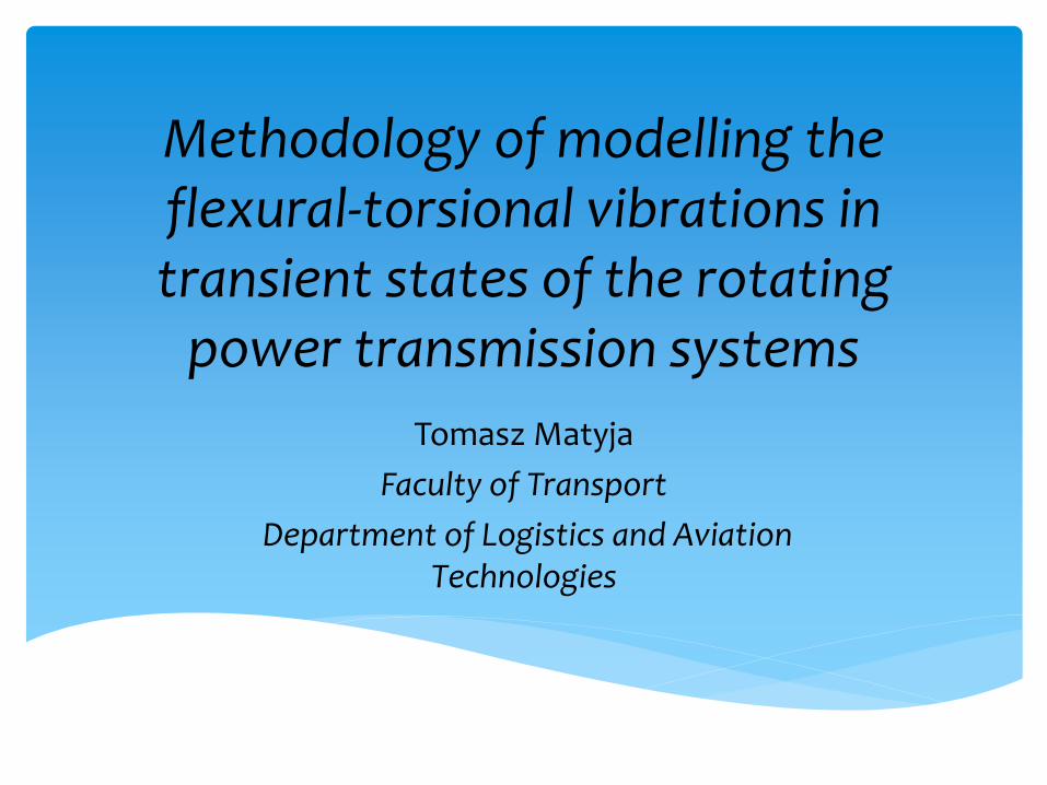
Rotating power transmission systems
2
Dynamic behaviors investigated by methods of Rotordynamics
Turbochargers
Ship shaft line
Helicopter drive system
Much more …
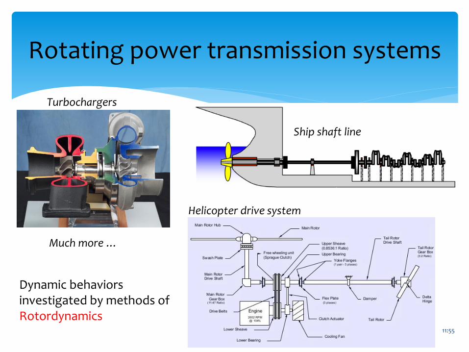
Motivation for research and work
Model of rigid rotor with six degrees of freedom
Decoupling equations of the rotor motion
Proposed decomposition method of the typical rotating system
Simulink library for modeling and simulation of dynamic phenomena in rotating power transmission systems
Examples of simulation studies
Conclusions
11:55
Plan of presentation
3
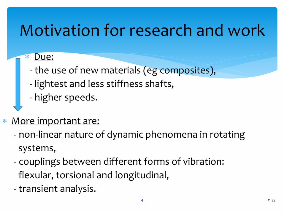
Due:
- the use of new materials (eg composites),
- lightest and less stiffness shafts,
- higher speeds.
11:55
Motivation for research and work
4
More important are:
- non-linear nature of dynamic phenomena in rotating
systems,
- couplings between different forms of vibration:
flexular, torsional and longitudinal,
- transient analysis.
11:55
Methods used in the Rotordynamics
5
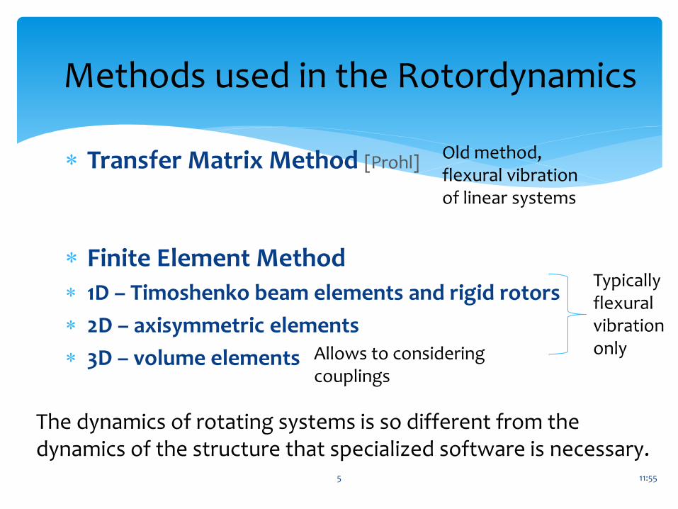
Transfer Matrix Method [Prohl]
Finite Element Method
1D – Timoshenko beam elements and rigid rotors
2D – axisymmetric elements
3D – volume elements
Typicallyflexuralvibrationonly
Old method, flexural vibration of linear systems
Allows to considering couplings
The dynamics of rotating systems is so different from the dynamics of the structure that specialized software is necessary.
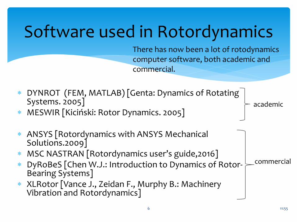
DYNROT (FEM, MATLAB) [Genta: Dynamics of RotatingSystems. 2005]
MESWIR [Kiciński: Rotor Dynamics. 2005]
ANSYS [Rotordynamics with ANSYS MechanicalSolutions.2009]
MSC NASTRAN [Rotordynamics user’s guide,2016] DyRoBeS [Chen W.J.: Introduction to Dynamics of Rotor-
Bearing Systems] XLRotor [Vance J., Zeidan F., Murphy B.: Machinery
Vibration and Rotordynamics]
11:55
Software used in Rotordynamics
6
academic
There has now been a lot of rotodynamicscomputer software, both academic and commercial.
commercial
11:55
Motivation for research and work
7
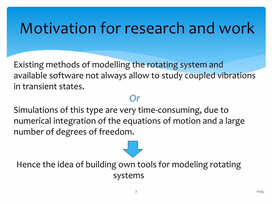
Existing methods of modelling the rotating system and available software not always allow to study coupled vibrations in transient states.
OrSimulations of this type are very time-consuming, due to numerical integration of the equations of motion and a large number of degrees of freedom.
Hence the idea of building own tools for modeling rotating systems
11:55
Model of rigid rotor with six degrees of freedom
8
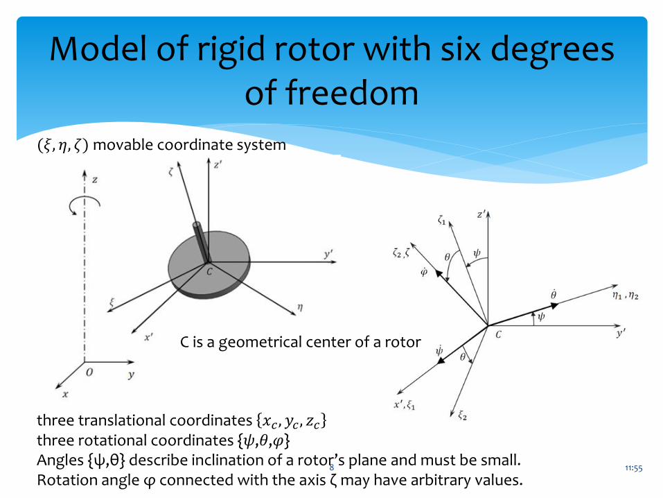
three translational coordinates 𝑥𝑐 , 𝑦𝑐 , 𝑧𝑐
three rotational coordinates {𝜓,𝜃,𝜑}Angles {ψ,θ} describe inclination of a rotor’s plane and must be small. Rotation angle φ connected with the axis ζ may have arbitrary values.
C is a geometrical center of a rotor
(𝜉, 휂, 휁) movable coordinate system
11:55
Selection of Euler angles (Rot 1-2-3) allows to avoid the „gimbal lock”
9
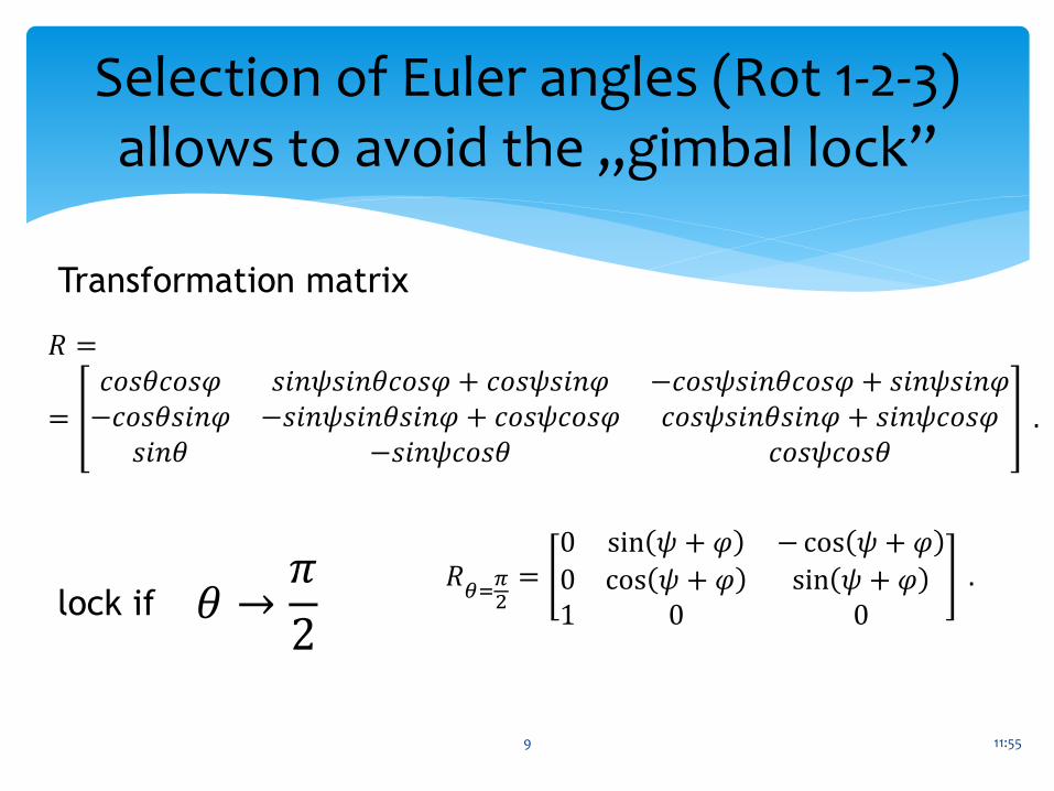
𝑅 =
=
𝑐𝑜𝑠휃𝑐𝑜𝑠𝜑 𝑠𝑖𝑛𝜓𝑠𝑖𝑛휃𝑐𝑜𝑠𝜑 + 𝑐𝑜𝑠𝜓𝑠𝑖𝑛𝜑 −𝑐𝑜𝑠𝜓𝑠𝑖𝑛휃𝑐𝑜𝑠𝜑 + 𝑠𝑖𝑛𝜓𝑠𝑖𝑛𝜑−𝑐𝑜𝑠휃𝑠𝑖𝑛𝜑 −𝑠𝑖𝑛𝜓𝑠𝑖𝑛휃𝑠𝑖𝑛𝜑 + 𝑐𝑜𝑠𝜓𝑐𝑜𝑠𝜑 𝑐𝑜𝑠𝜓𝑠𝑖𝑛휃𝑠𝑖𝑛𝜑 + 𝑠𝑖𝑛𝜓𝑐𝑜𝑠𝜑
𝑠𝑖𝑛휃 −𝑠𝑖𝑛𝜓𝑐𝑜𝑠휃 𝑐𝑜𝑠𝜓𝑐𝑜𝑠휃.
Transformation matrix
𝑅𝜃=
𝜋2
=0 sin 𝜓 + 𝜑 −cos 𝜓 + 𝜑
0 cos 𝜓 + 𝜑 sin 𝜓 + 𝜑1 0 0
.휃 →
𝜋
2lock if
11:55
Static and dynamic unbalance
10
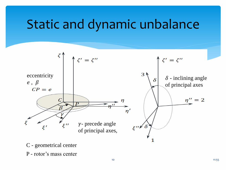
C - geometrical center
P - rotor’s mass center
𝛾- precede angle
of principal axes,
𝛿 - inclining angle
of principal axes
eccentricity
𝑒 , 𝛽
11:55
Inertia matrix of the rotor
11
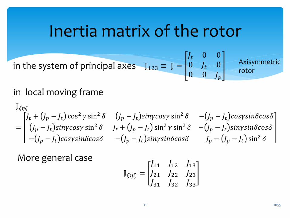
𝕁123 ≡ 𝕁 =
𝐽𝑡 0 00 𝐽𝑡 00 0 𝐽𝑝
𝕁𝜉𝜂𝜁
=
𝐽𝑡 + 𝐽𝑝 − 𝐽𝑡 cos2 𝛾 sin2 𝛿 𝐽𝑝 − 𝐽𝑡 𝑠𝑖𝑛𝛾𝑐𝑜𝑠𝛾 sin2 𝛿 − 𝐽𝑝 − 𝐽𝑡 𝑐𝑜𝑠𝛾𝑠𝑖𝑛𝛿𝑐𝑜𝑠𝛿
𝐽𝑝 − 𝐽𝑡 𝑠𝑖𝑛𝛾𝑐𝑜𝑠𝛾 sin2 𝛿 𝐽𝑡 + 𝐽𝑝 − 𝐽𝑡 sin2 𝛾 sin2 𝛿 − 𝐽𝑝 − 𝐽𝑡 𝑠𝑖𝑛𝛾𝑠𝑖𝑛𝛿𝑐𝑜𝑠𝛿
− 𝐽𝑝 − 𝐽𝑡 𝑐𝑜𝑠𝛾𝑠𝑖𝑛𝛿𝑐𝑜𝑠𝛿 − 𝐽𝑝 − 𝐽𝑡 𝑠𝑖𝑛𝛾𝑠𝑖𝑛𝛿𝑐𝑜𝑠𝛿 𝐽𝑝 − 𝐽𝑝 − 𝐽𝑡 sin2 𝛿
in the system of principal axes
in local moving frame
Axisymmetric rotor
More general case
𝕁𝜉𝜂𝜁 =
𝐽11 𝐽12 𝐽13
𝐽21 𝐽22 𝐽23
𝐽31 𝐽32 𝐽33
11:55
Lagrange equations of rotor motion
12
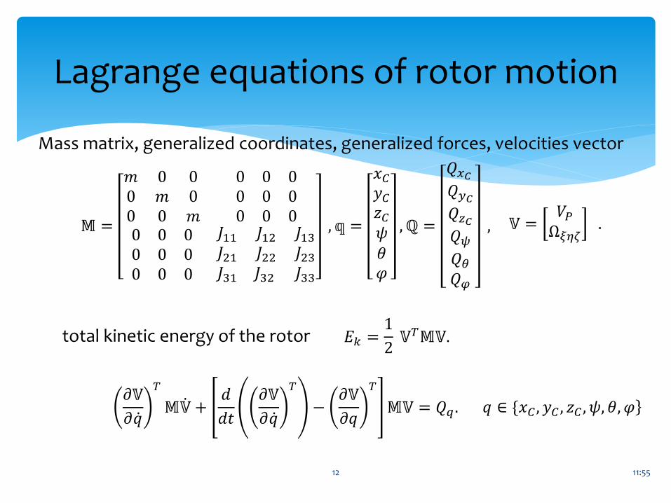
𝕄 =
𝑚 0 00 𝑚 00 0 𝑚
0 0 00 0 00 0 0
0 0 00 0 00 0 0
𝐽11 𝐽12 𝐽13
𝐽21 𝐽22 𝐽23
𝐽31 𝐽32 𝐽33
, 𝕢 =
𝑥𝐶
𝑦𝐶
𝑧𝐶
𝜓휃𝜑
,ℚ =
𝑄𝑥𝐶
𝑄𝑦𝐶
𝑄𝑧𝐶
𝑄𝜓
𝑄𝜃
𝑄𝜑
, 𝕍 =𝑉𝑃
Ω𝜉𝜂𝜁.
𝐸𝑘 =1
2𝕍𝑇𝕄𝕍.
𝜕𝕍
𝜕 𝑞
𝑇
𝕄 𝕍 +𝑑
𝑑𝑡
𝜕𝕍
𝜕 𝑞
𝑇
−𝜕𝕍
𝜕𝑞
𝑇
𝕄𝕍 = 𝑄𝑞 . 𝑞 ∈ {𝑥𝐶 , 𝑦𝐶 , 𝑧𝐶 , 𝜓, 휃, 𝜑
Mass matrix, generalized coordinates, generalized forces, velocities vector
total kinetic energy of the rotor
11:55
Inertia coupling equations
13
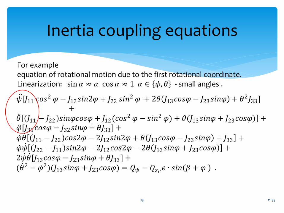
𝜓[ 𝐽11 𝑐𝑜𝑠2 𝜑 − 𝐽12𝑠𝑖𝑛2𝜑 + 𝐽22 𝑠𝑖𝑛2 𝜑 + 2휃(𝐽13𝑐𝑜𝑠𝜑 − 𝐽23𝑠𝑖𝑛𝜑) + 휃2𝐽33]+
휃 (𝐽11 − 𝐽22)𝑠𝑖𝑛𝜑𝑐𝑜𝑠𝜑 + 𝐽12(𝑐𝑜𝑠2 𝜑 − 𝑠𝑖𝑛2 𝜑) + 휃(𝐽13𝑠𝑖𝑛𝜑 + 𝐽23𝑐𝑜𝑠𝜑) + 𝜑 [𝐽31𝑐𝑜𝑠𝜑 − 𝐽32𝑠𝑖𝑛𝜑 + 휃𝐽33] + 𝜑 휃 (𝐽11 − 𝐽22)𝑐𝑜𝑠2𝜑 − 2𝐽12𝑠𝑖𝑛2𝜑 + 휃(𝐽13𝑐𝑜𝑠𝜑 − 𝐽23𝑠𝑖𝑛𝜑) + 𝐽33 + 𝜑 𝜓 (𝐽22 − 𝐽11)𝑠𝑖𝑛2𝜑 − 2𝐽12𝑐𝑜𝑠2𝜑 − 2휃(𝐽13𝑠𝑖𝑛𝜑 + 𝐽23𝑐𝑜𝑠𝜑) + 2𝜓 휃 [𝐽13𝑐𝑜𝑠𝜑 − 𝐽23𝑠𝑖𝑛𝜑 + 휃𝐽33] + (휃 2 − 𝜑 2)(𝐽13𝑠𝑖𝑛𝜑 + 𝐽23𝑐𝑜𝑠𝜑) = 𝑄𝜓 − 𝑄𝑧𝐶
𝑒 ∙ 𝑠𝑖𝑛(𝛽 + 𝜑 ) .
For exampleequation of rotational motion due to the first rotational coordinate.Linearization: sin 𝛼 ≈ 𝛼 cos 𝛼 ≈ 1 𝛼 ∈ 𝜓, 휃 - small angles .
11:55
Decoupling the equationsof the rotor motion
14
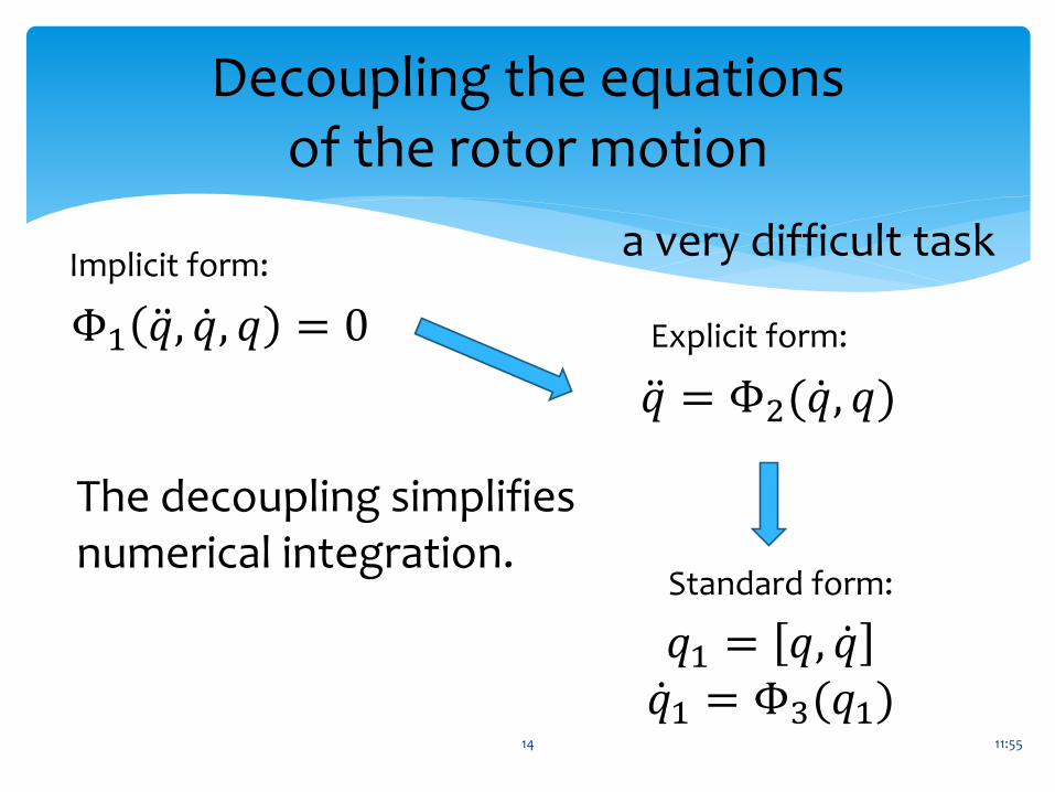
Φ1 𝑞, 𝑞, 𝑞 = 0
𝑞 = Φ2( 𝑞, 𝑞)
𝑞1 = 𝑞, 𝑞 𝑞1 = Φ3(𝑞1)
a very difficult taskImplicit form:
Explicit form:
Standard form:
The decoupling simplifies numerical integration.
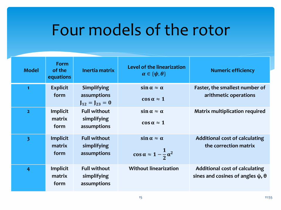
ModelForm
of the equations
Inertia matrixLevel of the linearization
𝜶 ∈ {𝝍, 𝜽 Numeric efficiency
1 Explicit
form
Simplifying
assumptions
𝐉𝟏𝟐 = 𝐉𝟐𝟑 = 𝟎
𝐬𝐢𝐧𝛂 ≈ 𝛂
𝐜𝐨𝐬𝛂 ≈ 𝟏
Faster, the smallest number of
arithmetic operations
2 Implicit
matrix
form
Full without
simplifying
assumptions
𝐬𝐢𝐧𝛂 ≈ 𝛂
𝐜𝐨𝐬𝛂 ≈ 𝟏
Matrix multiplication required
3 Implicit
matrix
form
Full without
simplifying
assumptions
𝐬𝐢𝐧𝛂 ≈ 𝛂
𝐜𝐨𝐬𝛂 ≈ 𝟏 −𝟏
𝟐𝛂𝟐
Additional cost of calculating
the correction matrix
4 Implicit
matrix
form
Full without
simplifying
assumptions
Without linearization Additional cost of calculating
sines and cosines of angles ψ, θ
11:5515
Four models of the rotor
11:55
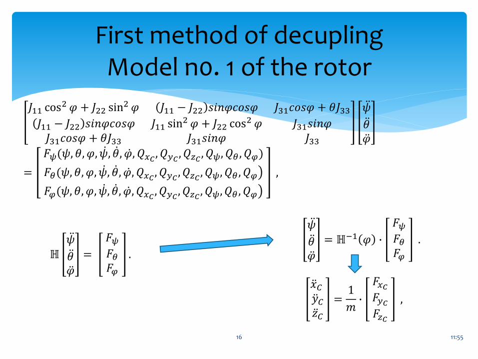
First method of decuplingModel n0. 1 of the rotor
16
𝐽11 cos2 𝜑 + 𝐽22 sin2 𝜑 𝐽11 − 𝐽22 𝑠𝑖𝑛𝜑𝑐𝑜𝑠𝜑 𝐽31𝑐𝑜𝑠𝜑 + 휃𝐽33
𝐽11 − 𝐽22 𝑠𝑖𝑛𝜑𝑐𝑜𝑠𝜑 𝐽11 sin2 𝜑 + 𝐽22 cos2 𝜑 𝐽31𝑠𝑖𝑛𝜑𝐽31𝑐𝑜𝑠𝜑 + 휃𝐽33 𝐽31𝑠𝑖𝑛𝜑 𝐽33
𝜓 휃 𝜑
=
𝐹𝜓(𝜓, 휃, 𝜑, 𝜓, 휃, 𝜑, 𝑄𝑥𝐶, 𝑄𝑦𝐶
, 𝑄𝑧𝐶, 𝑄𝜓, 𝑄𝜃 , 𝑄𝜑)
𝐹𝜃(𝜓, 휃, 𝜑, 𝜓, 휃, 𝜑, 𝑄𝑥𝐶, 𝑄𝑦𝐶
, 𝑄𝑧𝐶, 𝑄𝜓, 𝑄𝜃 , 𝑄𝜑
𝐹𝜑(𝜓, 휃, 𝜑, 𝜓, 휃, 𝜑, 𝑄𝑥𝐶, 𝑄𝑦𝐶
, 𝑄𝑧𝐶, 𝑄𝜓, 𝑄𝜃 , 𝑄𝜑
,
ℍ
𝜓 휃 𝜑
=
𝐹𝜓
𝐹𝜃
𝐹𝜑
.
𝜓 휃 𝜑
= ℍ−1 𝜑 ∙
𝐹𝜓
𝐹𝜃
𝐹𝜑
.
𝑥𝐶
𝑦𝐶
𝑧𝐶
=1
𝑚∙
𝐹𝑥𝐶
𝐹𝑦𝐶
𝐹𝑧𝐶
,
11:55
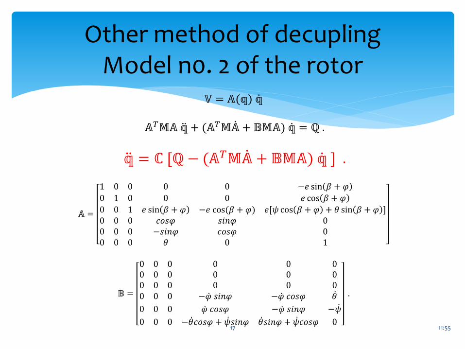
Other method of decuplingModel n0. 2 of the rotor
17
𝕍 = 𝔸(𝕢) 𝕢
𝔸𝑇𝕄𝔸 𝕢 + (𝔸𝑇𝕄 𝔸 + 𝔹𝕄𝔸) 𝕢 = ℚ .
𝕢 = ℂ ℚ − (𝔸𝑇𝕄 𝔸 + 𝔹𝕄𝔸) 𝕢 .
𝔸 =
1 0 0 0 0 −𝑒 sin 𝛽 + 𝜑
0 1 0 0 0 𝑒 cos 𝛽 + 𝜑
0 0 1 𝑒 sin 𝛽 + 𝜑 −𝑒 cos(𝛽 + 𝜑) 𝑒 𝜓 cos 𝛽 + 𝜑 + 휃 sin 𝛽 + 𝜑 0 0 0 𝑐𝑜𝑠𝜑 𝑠𝑖𝑛𝜑 00 0 0 −𝑠𝑖𝑛𝜑 𝑐𝑜𝑠𝜑 00 0 0 휃 0 1
𝔹 =
0 0 0 0 0 00 0 0 0 0 00 0 0 0 0 00 0 0 − 𝜑 𝑠𝑖𝑛𝜑 − 𝜑 𝑐𝑜𝑠𝜑 휃
0 0 0 𝜑 𝑐𝑜𝑠𝜑 − 𝜑 𝑠𝑖𝑛𝜑 − 𝜓
0 0 0 − 휃𝑐𝑜𝑠𝜑 + 𝜓𝑠𝑖𝑛𝜑 휃𝑠𝑖𝑛𝜑 + 𝜓𝑐𝑜𝑠𝜑 0
.
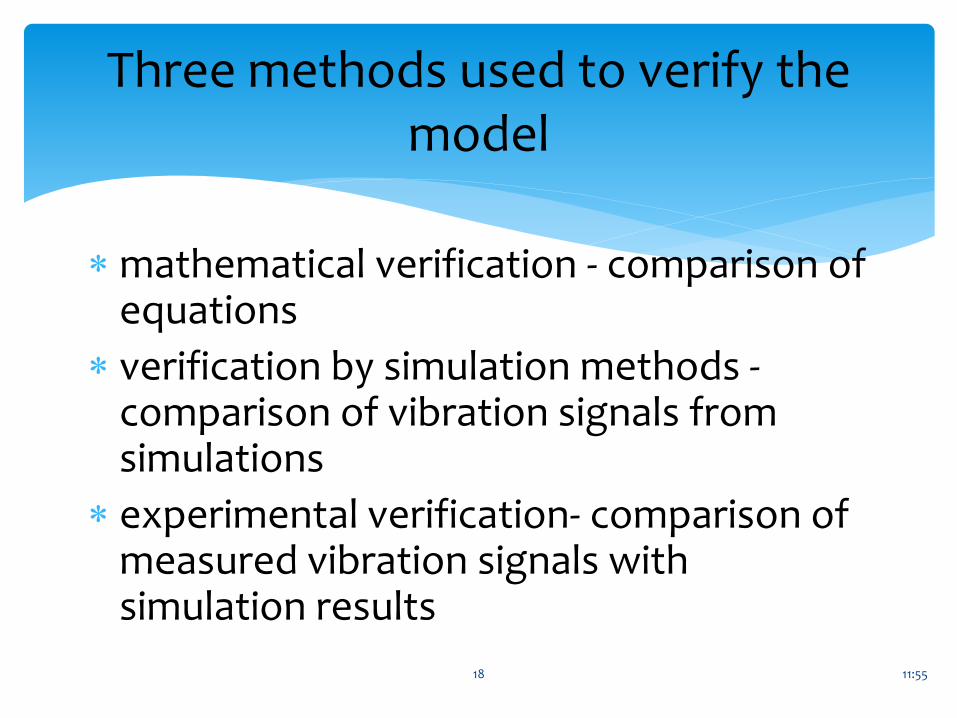
mathematical verification - comparison of equations
verification by simulation methods -comparison of vibration signals from simulations
experimental verification- comparison of measured vibration signals with simulation results
11:55
Three methods used to verify the model
18
11:55
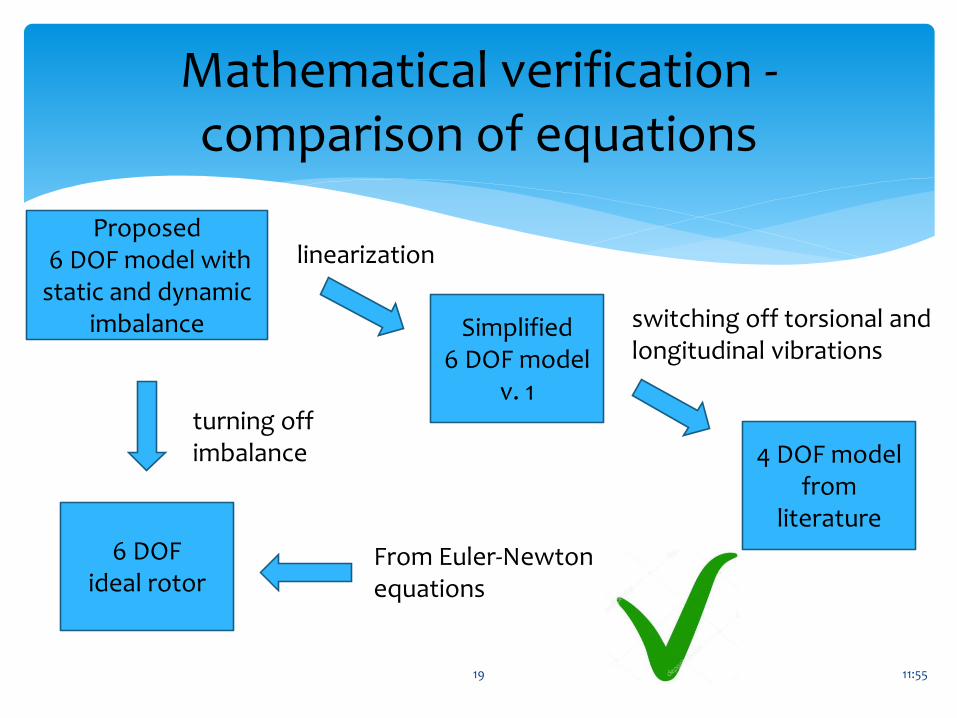
Mathematical verification -comparison of equations
19
Proposed6 DOF model with
static and dynamic imbalance Simplified
6 DOF model v. 1
4 DOF model from
literature
linearization
switching off torsional and longitudinal vibrations
6 DOFideal rotor
turning off imbalance
From Euler-Newtonequations
11:55
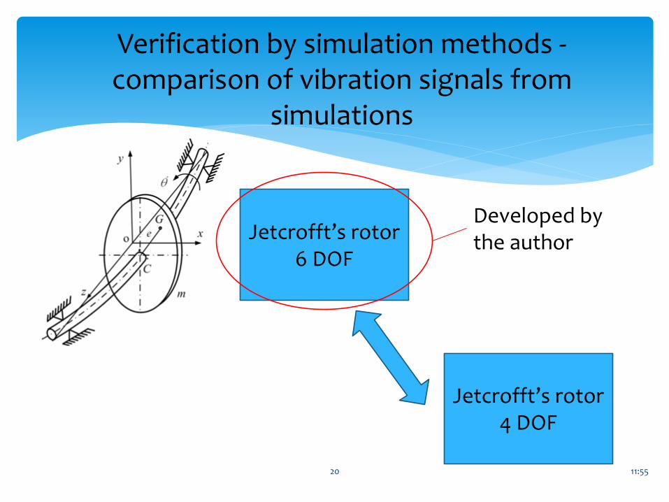
Verification by simulation methods -comparison of vibration signals from
simulations
20
Jetcrofft’s rotor6 DOF
Jetcrofft’s rotor4 DOF
Developed by the author
11:55
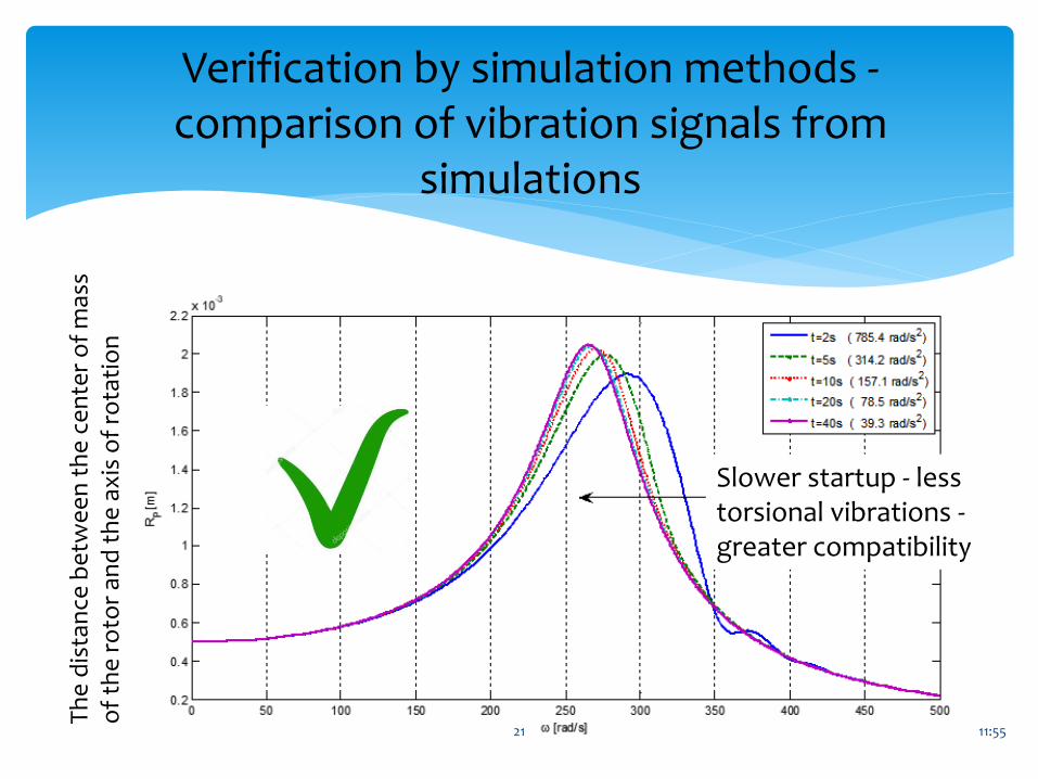
Verification by simulation methods -comparison of vibration signals from
simulations
21
Slower startup - less torsional vibrations -greater compatibility
Th
e d
ista
nce
be
twe
en
th
e c
en
ter
of
mas
s o
f th
e r
oto
r an
d t
he
ax
is o
f ro
tati
on
11:55
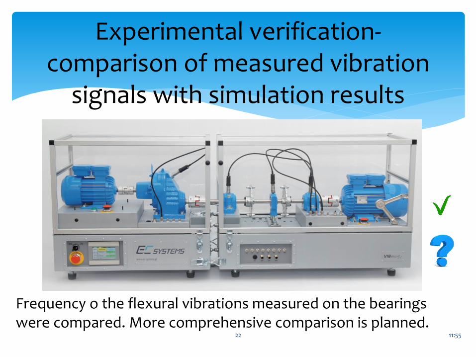
Experimental verification-comparison of measured vibration
signals with simulation results
22
Frequency o the flexural vibrations measured on the bearings were compared. More comprehensive comparison is planned.
11:55
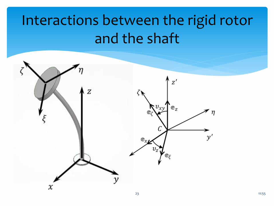
Interactions between the rigid rotor and the shaft
23
11:55
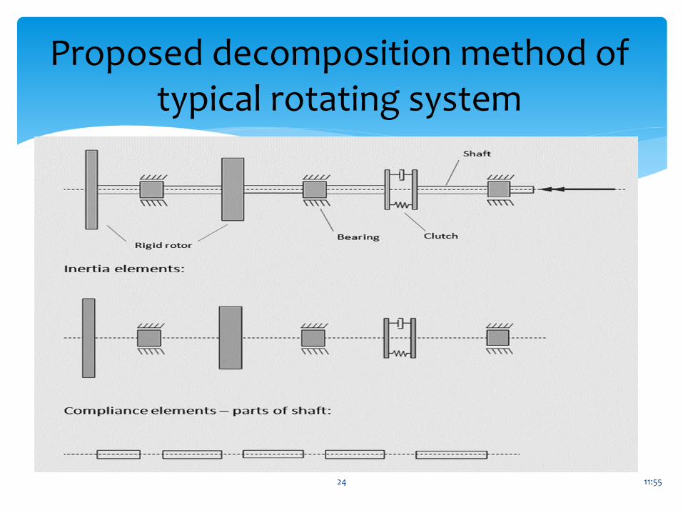
Proposed decomposition method of typical rotating system
24
11:55
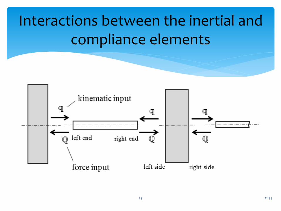
Interactions between the inertial and compliance elements
25
11:55
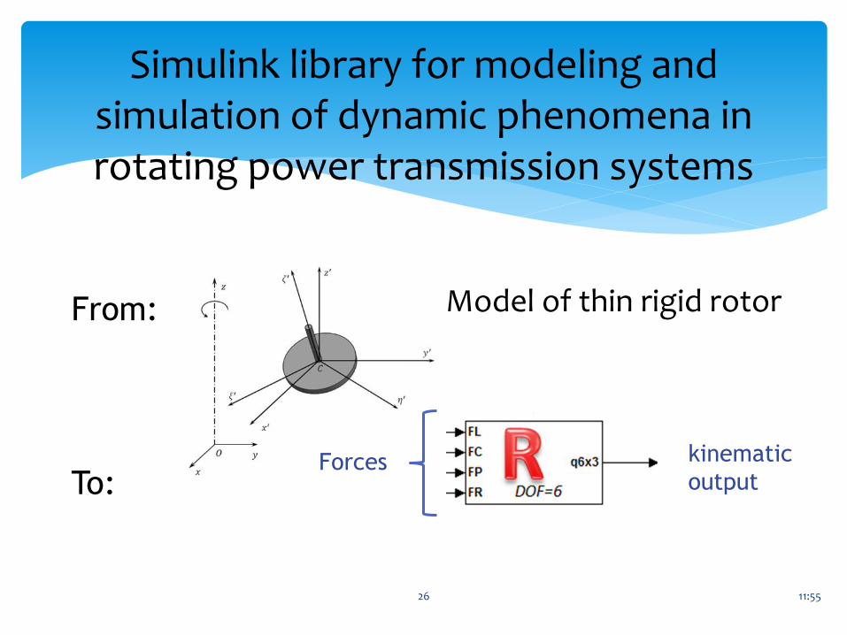
Simulink library for modeling and simulation of dynamic phenomena in rotating power transmission systems
26
Model of thin rigid rotorFrom:
To:Forces kinematic
output
11:55
Thin vs. Long Rotor
27
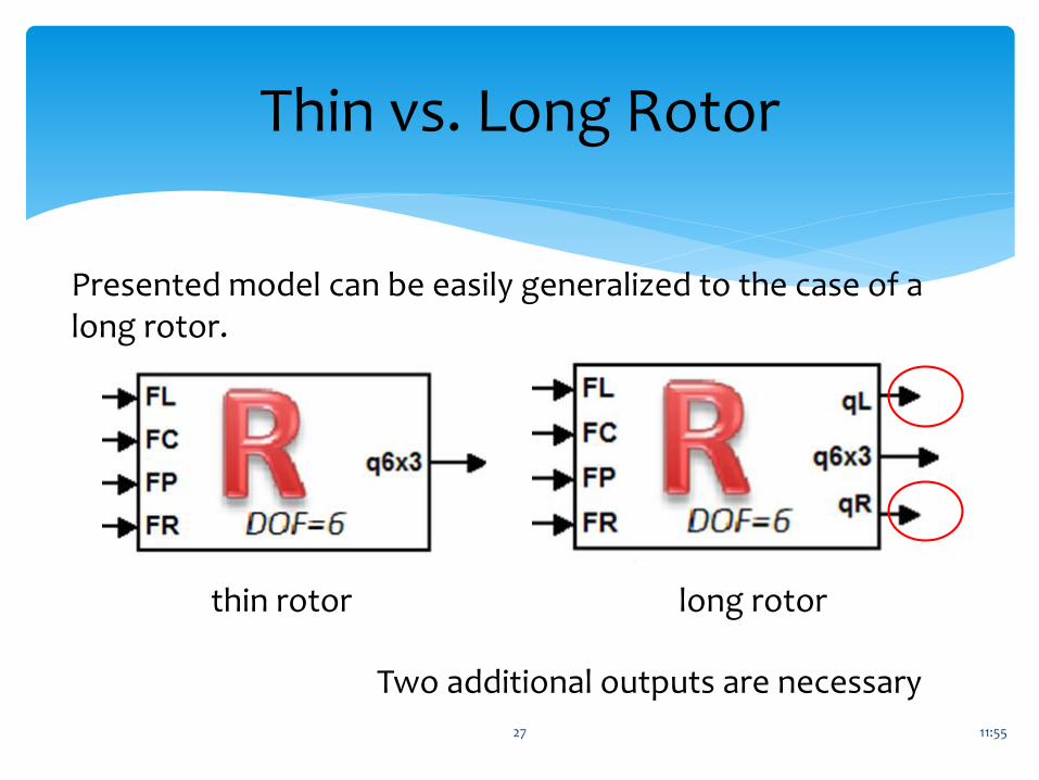
Presented model can be easily generalized to the case of a long rotor.
thin rotor long rotor
Two additional outputs are necessary
11:55
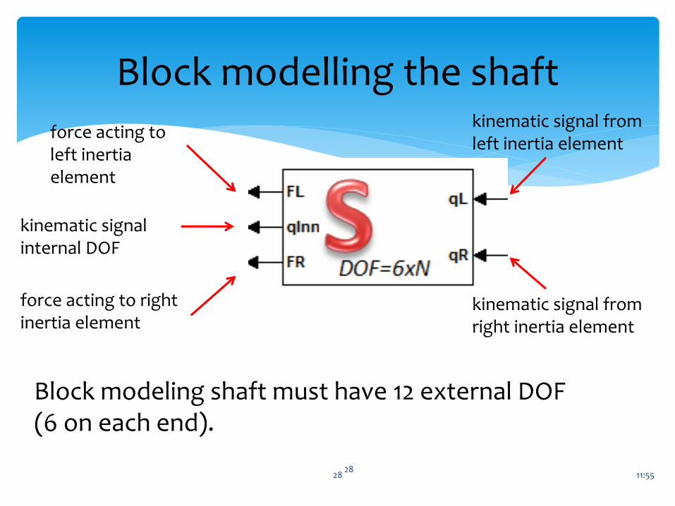
Block modelling the shaft
2828
kinematic signal from left inertia element
kinematic signal from right inertia element
kinematic signal internal DOF
force acting to left inertia element
force acting to right inertia element
Block modeling shaft must have 12 external DOF (6 on each end).
11:55
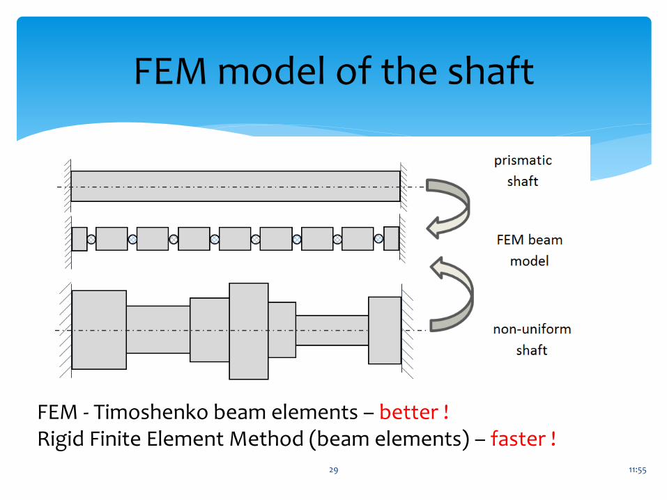
FEM model of the shaft
29
FEM - Timoshenko beam elements – better !Rigid Finite Element Method (beam elements) – faster !
11:55
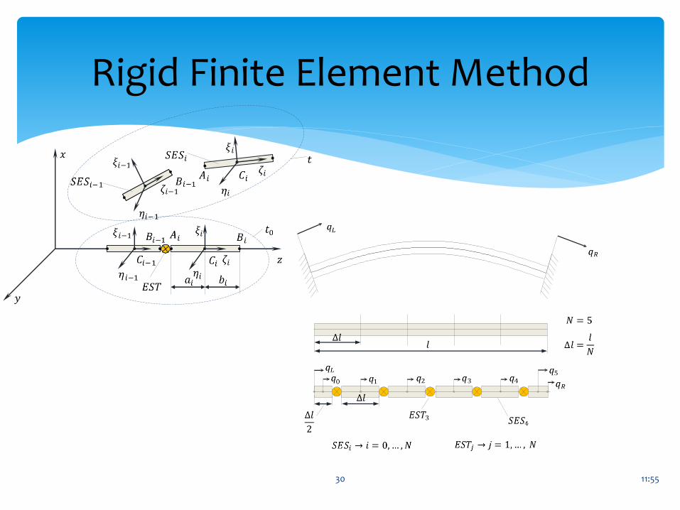
Rigid Finite Element Method
30
11:55
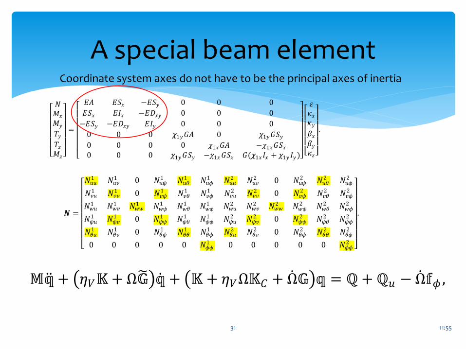
A special beam element
31
𝑵 =
𝑁𝑢𝑢
1 𝑁𝑢𝑣1 0 𝑁𝑢𝜓
1 𝑁𝑢휃1 𝑁𝑢𝜙
1 𝑁𝑢𝑢2 𝑁𝑢𝑣
2 0 𝑁𝑢𝜓2 𝑁𝑢휃
2 𝑁𝑢𝜙2
𝑁𝑣𝑢1 𝑁𝑣𝑣
1 0 𝑁𝑣𝜓1 𝑁𝑣휃
1 𝑁𝑣𝜙1 𝑁𝑣𝑢
2 𝑁𝑣𝑣2 0 𝑁𝑣𝜓
2 𝑁𝑣휃2 𝑁𝑣𝜙
2
𝑁𝑤𝑢1 𝑁𝑤𝑣
1 𝑁𝑤𝑤1 𝑁𝑤𝜓
1 𝑁𝑤휃1 𝑁𝑤𝜙
1 𝑁𝑤𝑢2 𝑁𝑤𝑣
2 𝑁𝑤𝑤2 𝑁𝑤𝜓
2 𝑁𝑤휃2 𝑁𝑤𝜙
2
𝑁𝜓𝑢1 𝑁𝜓𝑣
1 0 𝑁𝜓𝜓1 𝑁𝜓휃
1 𝑁𝜓𝜙1 𝑁𝜓𝑢
2 𝑁𝜓𝑣2 0 𝑁𝜓𝜓
2 𝑁𝜓휃2 𝑁𝜓𝜙
2
𝑁휃𝑢1 𝑁휃𝑣
1 0 𝑁휃𝜓1 𝑁휃휃
1 𝑁휃𝜙1 𝑁휃𝑢
2 𝑁휃𝑣2 0 𝑁휃𝜓
2 𝑁휃휃2 𝑁휃𝜙
2
0 0 0 0 0 𝑁𝜙𝜙1 0 0 0 0 0 𝑁𝜙𝜙
2
.
𝑁𝑀𝑥
𝑀𝑦
𝑇𝑦
𝑇𝑥
𝑀𝑧
=
𝐸𝐴 𝐸𝑆𝑥 −𝐸𝑆𝑦 0 0 0
𝐸𝑆𝑥 𝐸𝐼𝑥 −𝐸𝐷𝑥𝑦 0 0 0
−𝐸𝑆𝑦 −𝐸𝐷𝑥𝑦 𝐸𝐼𝑦 0 0 0
0 0 0 𝜒1𝑦𝐺𝐴 0 𝜒1𝑦𝐺𝑆𝑦
0 0 0 0 𝜒1𝑥𝐺𝐴 −𝜒1𝑥𝐺𝑆𝑥
0 0 0 𝜒1𝑦𝐺𝑆𝑦 −𝜒1𝑥𝐺𝑆𝑥 𝐺(𝜒1𝑥𝐼𝑥 + 𝜒1𝑦 𝐼𝑦 )
휀𝜅𝑥
𝜅𝑦
𝛽𝑥
𝛽𝑦
𝜅𝑧
.
𝕄𝕢 + 휂𝑉𝕂 + Ω𝔾 𝕢 + 𝕂 + 휂𝑉Ω𝕂𝐶 + Ω 𝔾 𝕢 = ℚ + ℚ𝑢 − Ω 𝕗𝜙 ,
Coordinate system axes do not have to be the principal axes of inertia
11:55
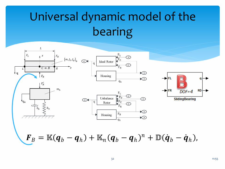
Universal dynamic model of the bearing
32
𝑭𝐵 = 𝕂(𝒒𝑏 − 𝒒ℎ) + 𝕂𝑛(𝒒𝑏 − 𝒒ℎ)𝑛 + 𝔻(𝒒 𝑏 − 𝒒 ℎ),

11:55
Universal dynamic model of the clutch
33
𝑭𝑊 = 𝑭𝑊(𝒒𝐿 , 𝒒 𝐿 , 𝒒𝑅 , 𝒒 𝑅),
11:55
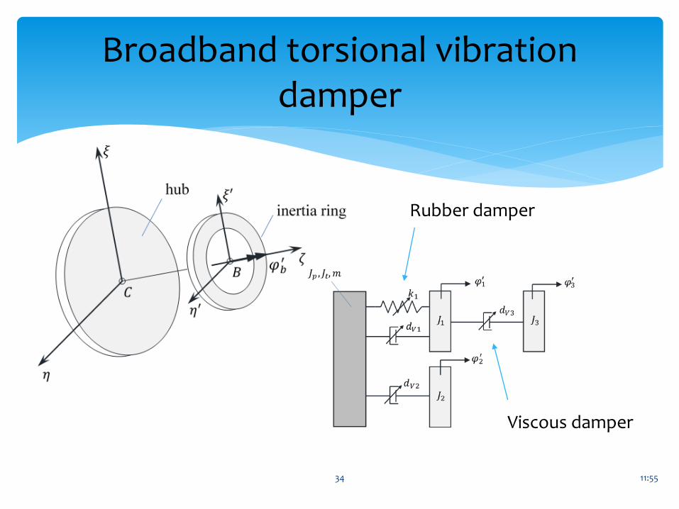
Broadband torsional vibration damper
34
Viscous damper
Rubber damper
11:55
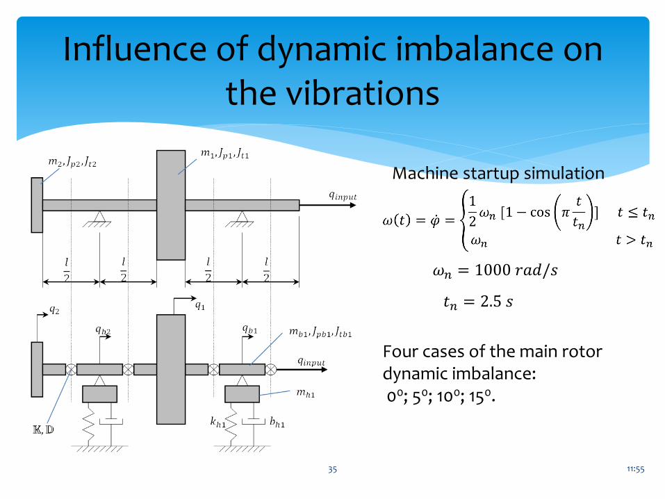
Influence of dynamic imbalance on the vibrations
35
Machine startup simulation
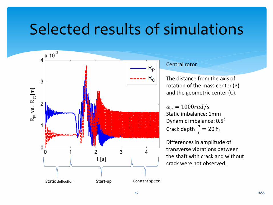
𝜔𝑛 = 1000 𝑟𝑎𝑑/𝑠
𝑡𝑛 = 2.5 𝑠
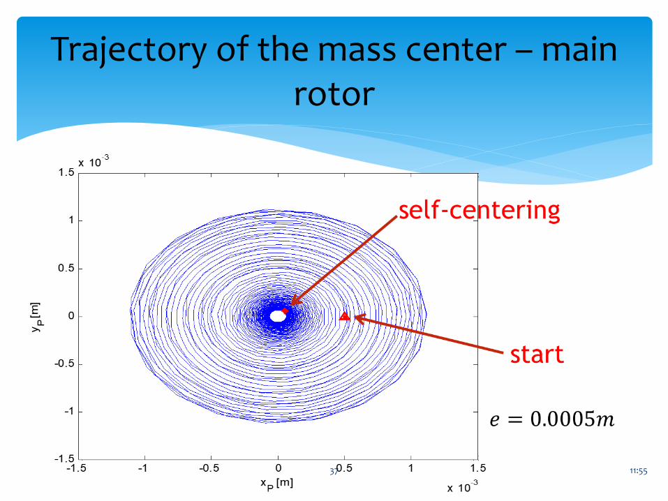
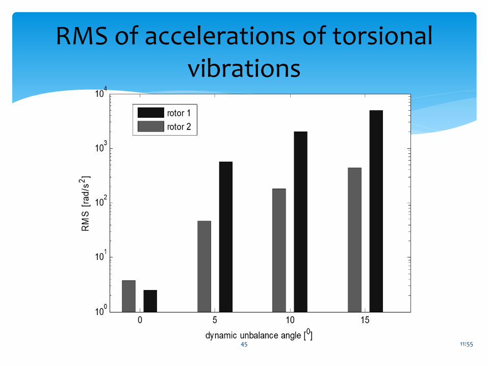
Four cases of the main rotor dynamic imbalance:00; 50; 100; 150.
11:55
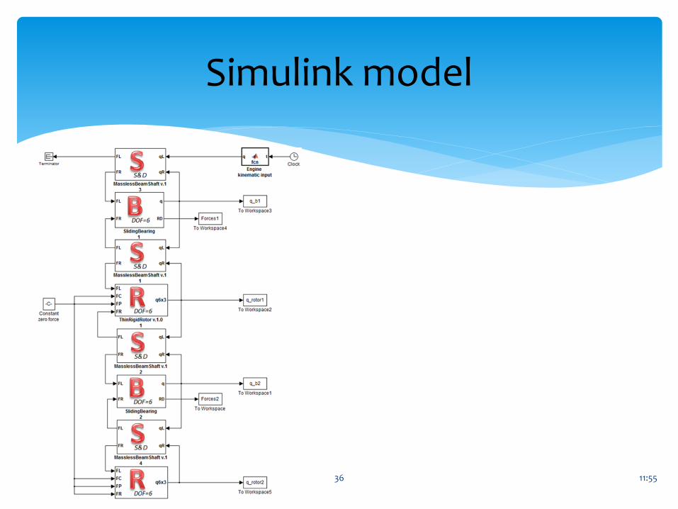
Simulink model
36
11:55
Trajectory of the mass center – main rotor
37
11:55
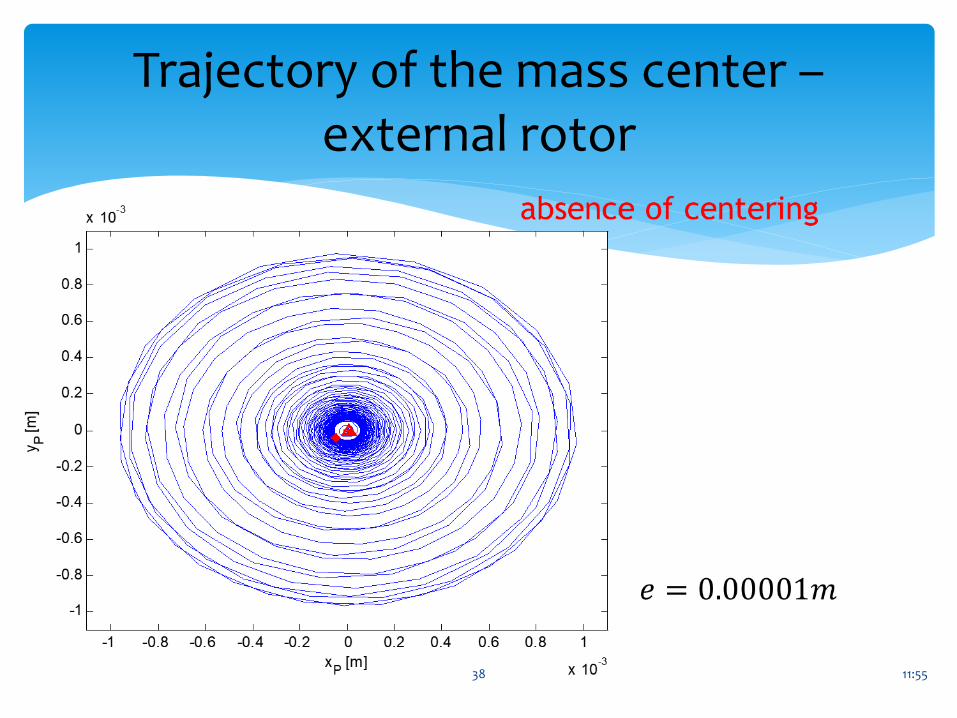
Trajectory of the mass center –external rotor
38
11:55
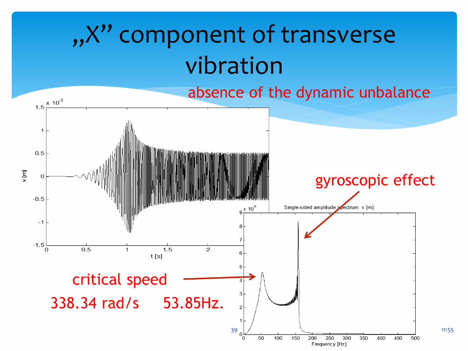
„X” component of transverse vibration
39

11:55
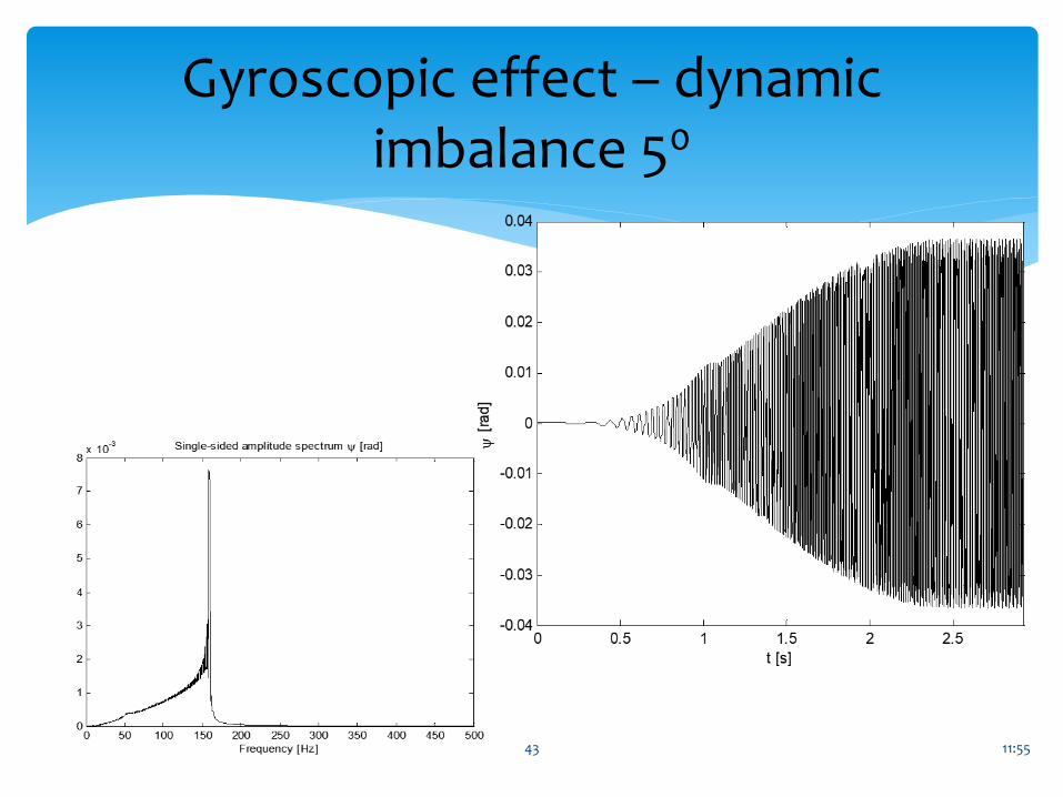
Gyroscopic effect - inclination angle of the rotor
40
11:55
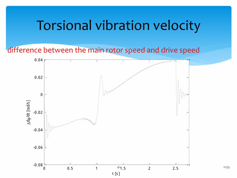
Torsional vibration velocity
410 0.5 1 1.5 2 2.5-0.08
-0.06
-0.04
-0.02
0
0.02
0.04
d
/dt
[rad/s
]
t [s]
difference between the main rotor speed and drive speed
11:55
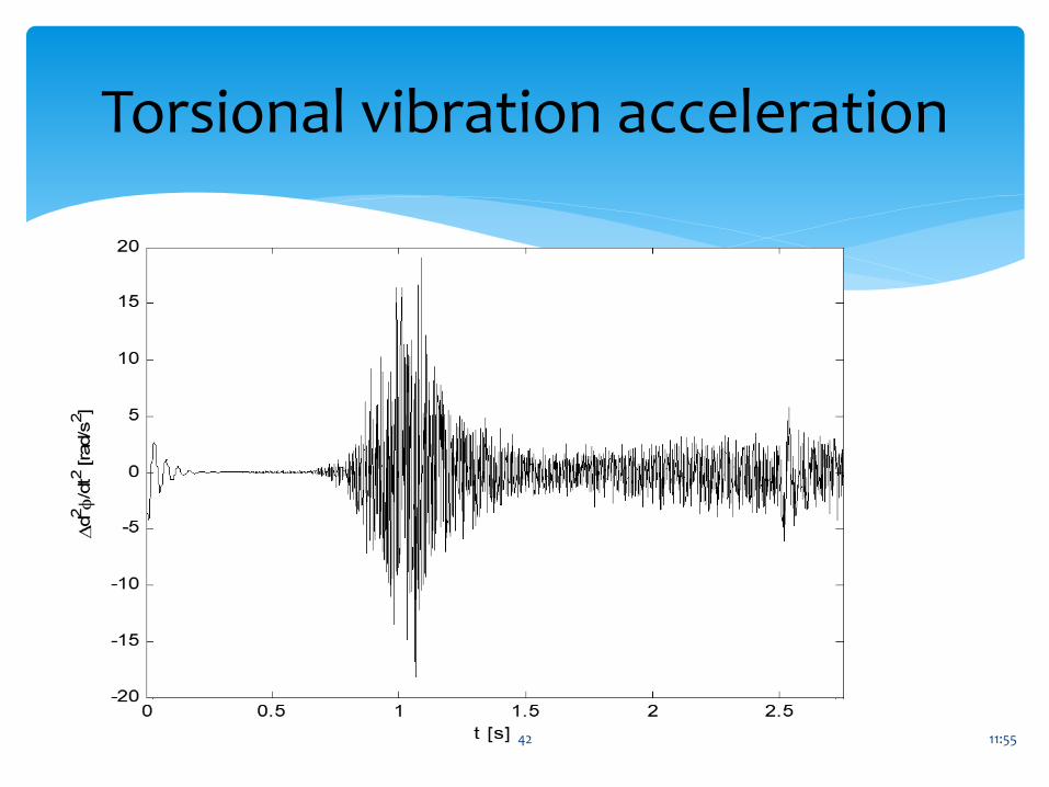
Torsional vibration acceleration
42
11:55
Gyroscopic effect – dynamicimbalance 50
43
11:55
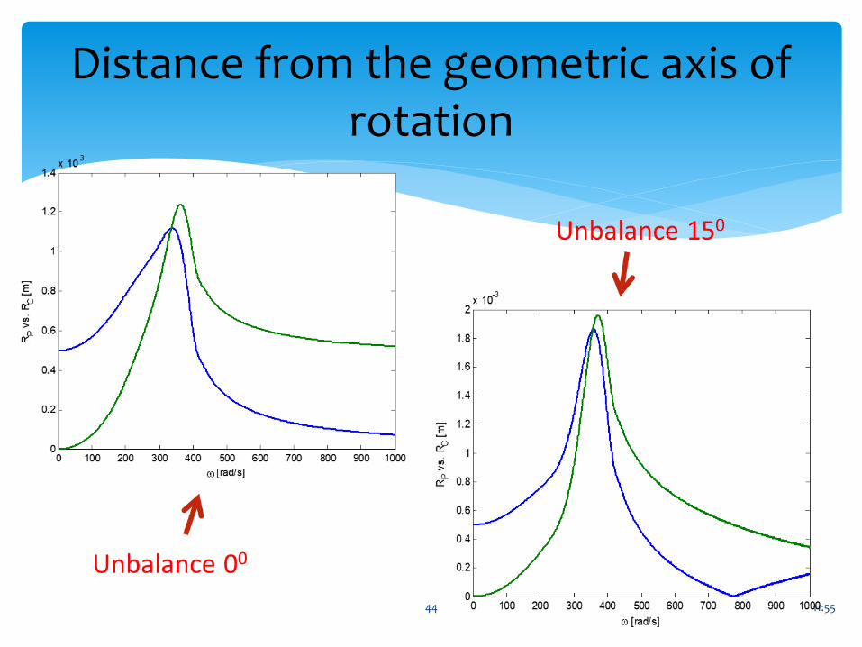
Distance from the geometric axis of rotation
44
11:55
RMS of accelerations of torsional vibrations
45
11:55
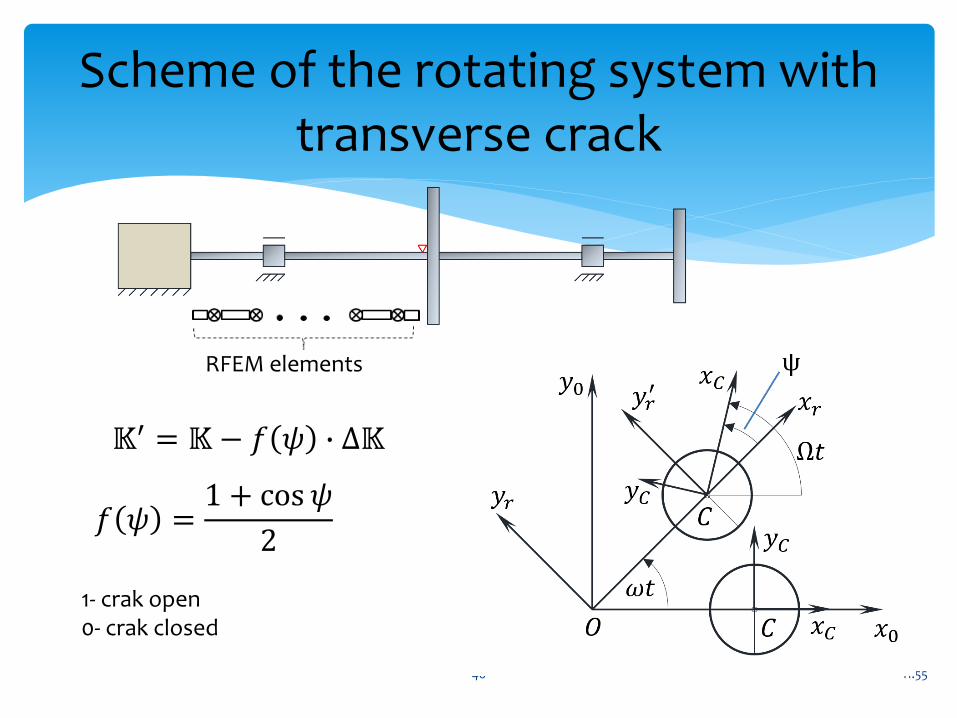
Scheme of the rotating system with transverse crack
46
𝕂′ = 𝕂 − 𝑓 𝜓 ∙ Δ𝕂
𝑓 𝜓 =1 + cos 𝜓
2
1- crak open0- crak closed
RFEM elements
11:5547
Selected results of simulations
11:5548
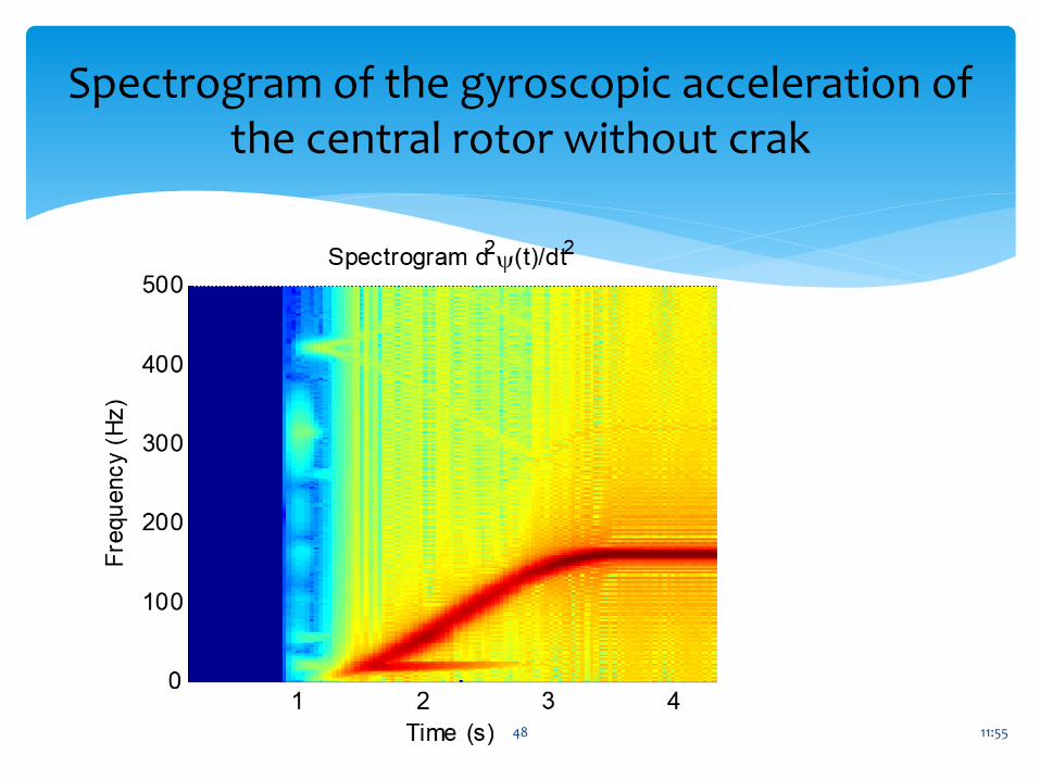
Spectrogram of the gyroscopic acceleration of the central rotor without crak

11:5549
Spectrogram of the gyroscopic acceleration of the central rotor with crak
• Presented method of modeling the rotating systems is an alternative to existing systems based on FEM.
• Its advantage is the relatively small number of degrees of freedom which reduces simulation time and allows to study non-steady states with low cost of computer hardware.
• The authors library of Simulink blocks can be freely expanded with new elements.
• Another advantage is ability to easily integrate with tools and models available in Simulink and Matlab.
11:5550
Conclusions
Thank you for your attention
11:5551