Methodology for Increasing the Measurement Accuracy of Image Features

Michael Majurski, Joe Chalfoun, Steven P. Lund, Peter Bajcsy, and Mary BradyNational Institute of Standards & Technology100 Bureau Drive, Gaithersburg, MD 20899

{michael.majurski, joe.chalfoun, steven.lund, peter.bajcsy, mary.brady}@nist.gov

Abstract

We present an optimization methodology for improvingthe measurement accuracy of image features for low signalto noise ratio (SNR) images. By superimposing known back-ground noise with high quality images in various propor-tions, we produce a degraded image set spanning a rangeof SNRs with reference feature values established from theunmodified high quality images. We then experiment with avariety of image processing spatial filters applied to the de-graded images and identify which filter produces an imagewhose feature values most closely correspond to the refer-ence values. When using the best combination of three fil-ters and six kernel sizes for each feature, the average cor-relation of feature values between the degraded and highquality images increased from 0.6 (without filtering) to 0.92(with feature-specific filters), a 53% improvement. Select-ing a single filter is more practical than having a separatefilter per feature. However, this results in a 1.95% reduc-tion in correlation and a 10% increase in feature residualroot mean square error compared to selecting the optimalfilter and kernel size per feature. We quantified the tradeoffbetween a practical solution for all features and feature-specific solution to support decision making.

1. IntroductionImage features are computed in cell biology to extract

quantitative information regarding cell state, differentiation,biological activity, and cell dynamics. The motivation forour work is the improvement of measurement accuracy forimage features extracted from time-lapse fluorescent im-ages of stem cell colonies. Due to cell sensitivity to light,only brief low intensity light could be used to excite fluo-rophores, producing images with low signal to noise ratios(SNRs) and hence resulting in questionable accuracy of im-age features.

Our objective is to mitigate the effects of image noiseon extracted features via image de-noising (filtering) withrespect to quantitative metrics. Quantitative imaging can

play an important role in scientific experiments as a meansto monitor and communicate behavior of complex systems(e.g. cell colonies) by recording features extracted from ob-jects of interest. An image feature is a function whose inputis an image. Ideally, the image itself is representative of thecurrent state of the biological system being imaged such thatchanges in the images are representative of changes in thesystem. In such cases, image features can provide usefulsummaries to help monitor and communicate the systemsbehavior. However, when images have a low SNR, poor fo-cus, or other distortions, the information extracted via fea-ture evaluation may not reflect the behavior of the underly-ing system. That is the ability to extract meaningful imagefeature values is linked to the quality of the acquired im-ages. Unfortunately, due to experimental constraints idealhigh quality images can be time consuming to acquire, im-practical, expensive, or damaging to the specimen. Thisforces the acquisition of lower quality images. Image pro-cessing algorithms can help mitigate measurement inaccu-racies caused by low quality images. The difficulty lies inselecting which image processing algorithms to apply fora given feature measurement. We are interested in deter-mining the ordered set of image processing operations thatresult in images whose feature values convey similar mean-ing to those of the same image if it was of higher quality, inother words, having clear signal and negligible noise.

In this paper, we focus on the effects of image noise,as opposed to other factors that may degrade image qual-ity. Image features measured from images with low SNRscan be very poorly correlated with ground truth feature val-ues, defined as those extracted from the same signal im-ages with minimal noise. Any conclusions and insightsbased upon those feature measurements can be unreliableand biased. As SNR decreases the meaningful signal varia-tions among the different images becomes lost to the noise.As a result, the extracted features begin to characterizethe behavior of the noise instead of the signal. Groundtruth features should be measured from very high SNRimages so feature values are predominantly a function ofsignal only, and minimally influenced by noise. Differ-

1

ent types of features might display various robustness tonoise. These effects should be investigated before inter-preting the features. Figure 1 shows the effect of im-age noise, displaying a feature value scatterplot for Tex-ture.Average.ENTROPY at an SNR of 2, plotting the mea-sured values against the ground truth values. The red y = xline with a slope of 45 ◦ denotes where the measured fea-ture value (y-axis) is equal to the ground truth feature value(x-axis). With a correlation value of ρ = 0.584 there isonly a vague linear relationship between the measured andground truth values. All features are drawn from Bajcsyet al. [1] and their mathematical definitions are available athttps://isg.nist.gov/deepzoomweb/stemcellfeatures.

Figure 1. Example low quality (SNR of 2) image feature measure-ments which do not correlate well with ground truth. The cor-relation (ρ) between measured and ground truth feature values is0.584. The red y = x line with a slope of 45 ◦ denotes where themeasured feature value (y-axis) is equal to the ground truth featurevalue (x-axis).

Previous research has addressed either image quality as-sessment or the accuracy of feature based application spe-cific results. The intermediate step of analyzing featurequality has been neglected. Image quality assessment uti-lizes two types of metrics, those based on quantitative de-viation from ground truth (SNR, PSNR, MSE [19]) andthose designed to mimic human visual perception (FSIM[19], RFSIM [18], MS-SSIM [15], SSIM [14]). In order toevaluate the quality of de-noised images researchers havecreated synthetic noise models and optimized the selec-tion of de-noising algorithms over using synthetic images[2, 6, 7, 11, 12, 13, 17]. In contrast, we leverage measuredimages, both high quality ground truth signal and noise. Wethen create evaluation data based only on measured images.Our methodology of operating on image features is less de-pendent upon the final application problem.

This paper presents an experimental optimizationmethodology for improving the measurement accuracy ofimage features. This methodology consists of four steps:(1) sequester a small subset of the specimen and acquirea set of reference signal images with the highest quality

(SNR) possible, (2) acquire a set of background noise im-ages typical of the target experiment, (3) combine the highquality images and the background noise images to create aset of pseudo-real images with an SNR typical of the targetexperiment, and (4) optimize the application of an orderedset of image processing algorithms in order to maximize thecorrespondence in feature values measured from the refer-ence signal images and the pseudo-real images.

The low SNR (pseudo-real) images mimic those of thetarget experiment but contain a known signal component.Therefore features computed from the pseudo-real imagescan be compared with features computed from the refer-ence signal images. This enables the design, optimiza-tion, and refinement of the target experiment image pro-cessing pipeline with respect to accurately measuring theimage features of interest. Figure 2 shows an overview ofthe proposed methodology. The reference signal and mea-sured noise images are combined into a pseudo-real imagetypical of the target experiment. Multiple image process-ing pipelines are applied to the pseudo-real image generat-ing processed images. Features are then extracted from theprocessed images and compared to feature values extractedfrom the reference signal images.

Figure 2. Overview of the methodology for improving the accu-racy of measured image features. The reference signal and mea-sured noise images are combined into a pseudo-real image typicalof the target experiment. The pseudo-real image is passed throughan image processing pipeline to generate a processed image. Fea-tures are extracted from the processed image and compared tofeatures extracted from the reference signal image, enabling theevaluation of several processing pipelines to determine which im-proves the accuracy of the extracted features best.

Pseudo-real images (created by combining measured im-ages) are preferable to synthetic images (created entirelyfrom computer simulation of signal and noise models) be-cause they are more relevant to the imaging experiment inquestion. Both pseudo-real images and synthetic images

contain a known signal component enabling comparison toground truth. However, the synthetic image noise modelmight not match the target imaging experiment. By relyingon experimentally observed reference signal and noise thepseudo-real images avoid this problem. The downside ofthe pseudo-real images is that any noise present in the ref-erence signal images cannot be overcome, setting an upperlimit on the improvement in feature measurement accuracy.By allowing the experimentalist to define the reference sig-nal and the expected noise the image quality model can bereduced to just SNR, assuming the selection of referencesignal images is such that the underlying population of sig-nal profiles is sufficiently narrow that the optimal filter isprincipally a function of SNR and not the signal itself. Incases where that is not true, the reference image set can berefined until the assumption is met. If required, this method-ology can be performed multiple times to optimize filter se-lection for each sub-type of signal. Other factors affectingfilter selection, which might be experiment dependent, willbe defined by the experimentalist as part of acquiring thereference signal and noise images.

2. MethodsThis experimental methodology for increasing image

feature measurement accuracy consists of two major stages.The first stage is the creation of the pseudo-real images andthe second stage is the optimization and evaluation of theimage processing required to increase the accuracy of themeasured image features in generated pseudo-real images.

2.1. Pseudo-Real Image Creation

In order to evaluate the accuracy of extracted image fea-tures, a known reference signal similar to ones own exper-iment is needed. Such a signal is acquired by imaging arepresentative subset of the experimental specimen with thehighest image quality possible. Since this sample is not be-ing relied upon for the actual experiment feature data, it isnot subject to the same experimental constraints which limitimage quality. For example, a longer exposure time thanis practical for the real experiment could be used. Thesehigh quality images are called the reference signal becausethey contain the reference foreground signal from which theground truth image features are extracted.

The next step is to acquire a sample of the backgroundnoise expected in the target experiment. These backgroundimages should mimic all noise sources in the target experi-ment while containing no foreground data. This is done byimaging a background area with the same acquisition setupas used in the actual experiment.

The pseudo-real images are created by combining thereference signal and measured background noise images.Thus the pseudo-real images mimic the expected target ex-periment images while containing a known reference signal

component. They are created by multiplying the referencesignal images by a scalar and then adding the backgroundnoise. The following procedure is used to create the pseudo-real images with a desired SNR.

1. Compute the mean of the foreground pixels (as iden-tified by segmentation), µF , from the reference signalimage, IF .

2. Compute the standard deviation of the background pix-els, σB , from the background noise image, IB .

3. Given a desired SNR value of k for the pseudo-realimage, compute the rescale factor (k ∗ σB)/µF .

4. Multiply the reference signal image by the rescale fac-tor then add the background images, Ik = k∗σB

µF×IF+

IB .

This pseudo-real image creation procedure is shown inFigure 3. The formula used to identify the rescale factorfor a specified SNR is derived from the Rose criterion asdescribed in [16].

Figure 3. Diagram outlining the pseudo-real image creation. Thereference signal (foreground) image is scaled by a factor (k ∗σB)/µF and added to the measured background noise image tocreate a pseudo-real image with a specified SNR value. Note: alldisplayed images were auto-contrasted using the same algorithmfor visual clarity.

2.2. Process Optimization

We then determine an ordered set of image processingoperations required to improve the feature measurement ac-curacy. Ground truth feature values are measured from thereference signal images, denoted Reference. These are thencompared with features measured from the pseudo-real im-ages after processing, denoted Processed. Correlation (ρ),described by Eq. (1), is used to compare sets of feature val-ues.

ρ =cov(Processed,Reference)

sd(Processed) ∗ sd(Reference)(1)

The correlation coefficient measures the linear relation-ship strength between the processed feature values and theircorresponding reference values. A correlation coefficient of1 indicates that there are scalar values a > 0 and b such thatthe equationReference = a∗Processed+b holds exactly.When primary interest lies in the relative sizes of pairwisedistances among any set of points, as opposed to the exactvalues of the features themselves, correlations near 1 can beinterpreted as meaning the two quantities are nearly equiv-alent.

3. Experimental Results

This section presents experimental results obtained byapplying the proposed optimization methodology to cellu-lar microscopy images. There are many factors involvedin keeping cells alive, but with respect to imaging, preven-tion of photo-toxicity is the important one. It is desirable tohave the highest SNR images possible to discern biologicalinformation with the highest fidelity. However, acquiringthese high SNR images requires exciting the fluorophoreswithin the cells with high-intensity light. This exposuredamages or kills the cells (due to photo-toxicity) and causesaccelerated photo-bleaching of the specimen. Note that weare mainly concerned with fluorescent imaging modalitieswhere the sample must be probed with excitation light. Fortransmitted light modalities photo-toxicity is less of a con-cern. Thus, our primary interest lies in strategies to bal-ance the competing interests of using minimally invasiveimaging techniques to avoid affecting cell behavior or sur-vival and acquiring high quality images which contain therequired information.

3.1. Measured Microscopy Images of Cells

The target imaging experiment consists of a time-lapseacquisition of the H9 human embryonic stem cell (hESC)line over the course of 5 days on a microscope equippedwith a controlled environment incubation chamber (KairosInstruments LLC, Pittsburgh, PA). This cell line was en-gineered to produce green fluorescent protein (GFP) underthe influence of the native OCT-4 promoter using a pub-lished homologous recombination plasmid construct devel-oped by the James Thomson lab [20] and obtained from Ad-dgene (Addgene, Cambridge, MA). Experimental imagingis performed using a Zeiss 200M microscope (Carl ZeissMicroscopy, LLC, Thronwood, NY) every 45 minutes via aCoolsnap HQ camera (Photometrics, Tucson, AZ) in a gridof 16×22 field of views (FOVs) with 10% overlap coveringapproximately 180 mm2. Each individual FOV (image) is1040× 1392 pixels.

The individual target experiment images are stitched intoa single mosaic per time point using MIST (Microscopy Im-age Stitching Tool) [3]. Foreground and background masksare generated by segmenting the phase-contrast stitchedimages using the Empirical Gradient Threshold technique[5]. The stitched mosaic images are flat-field corrected andbackground subtracted [4]. Using the foreground masks aset of 61 intensity and texture image features, taken from[1], are extracted from each colony. The intensity featuresare statistical moments: mode, mean, mode, standard devia-tion, skewness, kurtosis, etc. The texture features are basedon Haralick texture features [10] which generate four val-ues per feature type, the average amplitude, principle com-ponent angle, orthogonal component angle, and principlecomponent value.

Since this is a time-lapse experiment, the cells need tobe kept alive and minimally disturbed by the high intensitylight used in imaging. Therefore, experimental conditionsconstrain imaging to phase contrast (less-damaging trans-mitted light) and low SNR fluorescent imaging. Many re-gions of interest exhibit SNRs of roughly 2. The goal of thecell imaging is to classify stem cell colonies based on homo-geneity and to analyze the homogeneity distribution of thesecolonies through time. The classification of cell colonies isbased on the intensity and texture features extracted fromthe fluorescent images. Therefore, it is important to com-pute the features with the highest accuracy possible underthese circumstances. We apply the proposed methodologyon this problem to find the optimal image processing stepsthat increase the accuracy of the measured features.

3.2. Pseudo-Real Image Creation

For this application the reference signal image datasetconsists of 100 stem cell colonies imaged in the fluorescentchannel with a long exposure time and high power exci-tation light to create very high SNR images. All of thesecolonies fit within a single FOV and are larger than 1000pixels in area. It is important to note that in acquiring theseimages with the aforementioned acquisition parameters, thecolonies were both damaged and photo-bleached, makingthis acquisition method unsuitable for the target time-lapseexperiment.

Typical background noise for the target experiment is ac-quired by imaging the specimen background consisting ofcell culture media, culture dish, and any extracellular ma-trix protein coatings under the same acquisition parametersas the real experiment. In addition to any background auto-fluorescence, the CCD camera noise is captured in thesebackground images. We acquired 30 background imageswith different spatial locations on the plate typical of theconditions expected in the target time-lapse imaging exper-iment.

Conditional random sampling is applied to the set of

100 reference signal colony images and 30 measured back-ground noise images to produce the set of pseudo-real im-ages. Each colony image is combined with 3 backgroundimages. Each background image is selected 10 times fora total of 300 combinations. The subsampling, as opposedto a complete factorial design, is used to restrict computa-tional requirements to a reasonable level. Next, each colonyimage containing ideally pure signal is combined with itsselected backgrounds to create 5 target SNR levels (1, 2,4, 8, and 16). The colony images were segmented using amanually selected threshold (foreground is greater than 500intensity units) to set the background of the image to 0. Be-fore this adjustment the reference signal image background(non-colony pixels) contained just dark current noise fromthe CCD camera with intensity values of approximately 200units. The colony foreground contains pixels of approxi-mately 4000-8000 grayscale intensity units coming from a14bit CCD camera with an output range of 0-16284 inten-sity units.

3.3. Optimization of Image Processing Filters

For this application we are interested in selecting the spa-tial image processing filter and kernel size for each featurewhich produces the most accurate measurement of that fea-ture. While this methodology enables the design and op-timization of arbitrary image processing pipelines with re-spect to feature measurement accuracy, we have limited thecomplexity of the processing pipeline to a depth of one op-eration and a small set of manually selected spatial imagefilters (Average, Median, or Gaussian) [8, 9]. These fil-ters were chosen because they are commonly used methodsof reducing image noise. Each filter is parameterized by akernel size of which six were tested (3x3, 5x5, 7x7, 9x9,13x13, 17x17). In order to evaluate the image processing,each feature was computed for each combination of filtertype and kernel size.

3.4. Numerical Results

Each filter and kernel size combination is applied to thepseudo-real images and all 61 features are extracted fromthe processed images. This enables the analysis of howthe feature values change as a function of the image filter,kernel size, and image SNR. The target experiment of thisstudy has an expected image SNR of 2. The optimal filterand kernel size can be selected for each feature by selectingthe filter and kernel which maximizes the correlation in Eq.(1) between the processed and reference feature values.

Applying the filter selected for each feature increases theaverage correlation from 0.601 to 0.919. Of the 61 featuresevaluated, 77% are optimized with the Gaussian filter, 18%with the Average filter, 3.3% with the Median filter, and1.6% with No Filter. Kernel sizes 5x5 and 7x7 are the mostcommon at 20% and 61% respectively. The majority of the

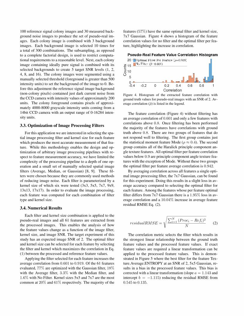
features (57%) have the same optimal filter and kernel size,7x7 Gaussian. Figure 4 shows a histogram of the featurecorrelation values for no filter and the optimal filter per fea-ture, highlighting the increase in correlation.

Figure 4. Histogram of the extracted feature correlation withground truth values for pseudo-real images with an SNR of 2. Av-erage correlation (ρ) is listed in the legend.

The feature correlation (Figure 4) without filtering hasan average correlation of 0.601 and only a few features withcorrelations above 0.8. Once filtering has been performedthe majority of the features have correlations with groundtruth above 0.8. There are two groups of features that donot respond well to filtering. The first group contains justthe statistical moment feature Mode (ρ ≈ 0.4). The secondgroup contains all of the Haralick principle component an-gle texture features. All optimal filter per feature correlationvalues below 0.9 are principle component angle texture fea-tures with the exception of Mode. Without these two groupsthe optimal filter per feature average correlation is 0.942.

By averaging correlation across all features a single opti-mal image processing filter, the 7x7 Gaussian, can be foundfor this experiment. Doing this results in a slight loss in av-erage accuracy compared to selecting the optimal filter foreach feature. Among the features whose per feature optimalfilter differs from 7x7 Gaussian there is a 1.95% loss in av-erage correlation and a 10.04% increase in average featureresidual RMSE Eq. (2).

residualRMSE =

√∑Ni=1 (Proci −Refi)2

N(2)

The correlation metric selects the filter which results inthe strongest linear relationship between the ground truthfeature values and the processed feature values. If exactfeature values are required a linear transformation can beapplied to the processed feature values. This is demon-strated in Figure 5 where the best filter for the feature Tex-ture.Average.ENTROPY at an SNR of 2, 5x5 Gaussian, re-sults in a bias in the processed feature values. This bias iscorrected with a linear transformation (slope a = 1.143 andintercept b = −1.115) reducing the residual RMSE from0.545 to 0.135.

Figure 5. Feature Texture.Average.ENTROPY (SNR of 2) pro-cessed with the 5x5 Gaussian filter. The original processed featurevalues are shown in (a) with a bias residual RMSE of 0.545. Thelinear transformation of the processed feature values is shown in(b) with a lower residual RMSE value of 0.135.

To examine the relationships between the processed im-age feature values and the ground truth feature values a se-ries of exploratory plots were generated. The first, shownin Figure 6, contains scatterplots of the processed featurevalues plotted against the ground truth feature values. Thisfigure is organized into a two dimensional grid of scatter-plots. Within each plot the feature value for an individualimage is shown as a single point and the line marks y = x,where the processed value equals the reference value. Thetext superimposed on each scatterplot is the correspondingcorrelation coefficient, see Eq. (1).

With no filter applied (indicated by the 1x1 kernel size)there is a clear bias in the computed features that decreaseswith processing. As the kernel size increases the correla-tion values increase and the feature values show a reduc-tion in bias. The effects of different image filter types ismost evident in the 3x3 kernel size plots. Of the 3x3 filters,the Average filter has th least bias and highest correlation.Moving across the row of 3x3 kernel size scatterplots, thecorrelation decreases and the distribution gets further fromthe y = x line. Increasing the kernel size reduces the dis-parity in results between filter types. The optimal filter forthis feature is Gaussian with kernel size 5x5.

Due to the high dimensionality of the feature accuracydata it is hard to conceptualize the full picture. Therefore, asummary plot was created where the correlation values pre-viously printed on the scatterplot are plotted as a functionof image feature, filter type, kernel size, and image SNR.This plot is shown in Figure 7 and can be found in sup-plementary document 1. Each image SNR block contains4 sub-blocks, the Gaussian filter block ’Gau’, the Medianfilter block ’Med’, the Average filter block ’Ave’, and theNo filter block ’None’. Within each filter block, the ker-nel size increases from bottom to top, 3 to 17. Per columnwithin each SNR block the maximum correlation value isshown by printing the relevant kernel size. Figure 7 showsthat there is considerable variability in the optimal filter andkernel size between different features. Overall, as the imageSNR increases the optimal kernel sizes shrink.

Figure 6. Feature value scatterplots for the feature Tex-ture.Average.Entropy at an SNR of 2 given the different filter typesand kernel sizes. This figure is organized into a two dimensionalgrid of plots. Within each plot the feature value for an individualimage is shown as a single point. The line marks y = x, wherethe processed feature value equals the reference feature value. Thesuperimposed text on each scatterplot is the correlation coefficient(ρ) for that scatterplot.

Reducing the dimensionality of the data once more isdone by averaging correlation values across all features toproduce a single value per filter type, image SNR, and ker-nel size. This creates plots where feature correlation isshown as a function of kernel size for each image SNR andfilter type. Figure 8 depicts plots of these feature correla-tions processed with Average, Median, and Gaussian filters,where each point shows correlation averaged across all 61features.

4. Discussion

There are several general observations that can begleaned from Figure 8. First, a dominant factor in deter-mining the processed feature measurement accuracy is theimage SNR. The higher the acquired image SNR the moreaccurate the feature measurement which is logical sincehigher SNRs have less noise to distort the feature measure-

Figure 7. Correlation summary plot. Each image SNR block contains 4 sub-blocks, the Gaussian filter block ’Gau’, the Median filter block’Med’, the Average filter block ’Ave’, and the No filter block ’None’. Within each filter block, the kernel size increases from bottom totop, 3 to 17. Per column within each SNR block the maximum correlation value is shown by printing the relevant kernel size.

ments. If the image SNR is high enough there is little to noaccuracy gained by filtering the images. For example, at anSNR of 16 a 3x3 kernel provides a minor increase in featuremeasurement accuracy, but a 5x5 kernel provides equal orworse accuracy than no filter. Second, as the image SNRdecreases, larger filter kernels are required to obtain a givenlevel of feature measurement accuracy. For example, at anSNR of 4 a 3x3 Gaussian kernel produces roughly the sameaccuracy as a 5x5 Gaussian kernel at an SNR of 2. Third,Gaussian filters require a larger kernel size to accomplishthe same effect as the Median or Average filters.

The time-lapse stem cell colony imaging experiment pre-sented here has an SNR of approximately 2. Given thatconstraint, the optimal image filter and kernel size for eachfeature should be selected such that the correlation betweenthe processed feature values and ground truth feature valuesis maximized. The per feature filter selection accuracy datais available in supplementary document 2 for each imageSNR level. Looking at just the filter type selection for anSNR of 2, 77% are optimized with the Gaussian filter, 18%with the Average filter, 3.3% with the Median filter, and1.6% with No Filter. The optimal kernel size distribution is

Figure 8. Average feature correlation values for each Filter, SNR, and Kernel size combination. The first plot was processed with anAverage filter, the second a Median filter, and the third a Gaussian filter. Within each plot correlation is shown as a function of kernel sizefor multiple SNR values.

more spread out with 60.65% being 7x7, 19.67% 5x5, 8.2%3x3, 6.56% 9x9, 3.23% 13x13, 1.64% No Filter, and 0.0%17x17. The most common filter and kernel size combina-tion is 7x7 Gaussian which is optimal for the majority ofthe features (57%). This effect shows up in Figure 7 as afairly consistent row of ’7’s written within the ’Gau’ blockof ’SNR=2’.

Texture features which compute a principle componentdirectionality angle did not improve nearly as much as theother evaluated features. These features accounted for allbut 1 of the features that did not obtain a correlation of 0.9or greater under any considered filter. This shows up in Fig-ure 7 as a vertical block of lower correlation values acrossall SNRs.

Whether one selects a single image processing filter forthe entire experiment or a filter per feature, these resultsare only relevant for the target experiment under consider-ation. The numerical results cannot be generalized but themethodology can. Changes in the target experiment (dif-ferent cell line, different features, etc.) would require thispre-experiment to be redone in order to find the optimal fil-ter(s) and kernel size(s) for the new target experiment. Thepower of this approach is its flexibility and extensibility.This optimization methodology can be applied to differentexperiments, image conditions, image modalities, and im-age features. For small scale experiments it might not bereasonable to perform such a pre-experiment to help designthe target experiment and its data processing. However, aslong as the pre-experiment does not constitute an unreason-able effort, it can help inform the accuracy of the target ex-periment.

5. Conclusions

This work was motivated by a desire to understand theimpact on stem cell colony classification when using im-age features derived from low SNR images. We devised amethodology to quantify the improvement of feature mea-

surement for a given image pre-processing method. As aproof of concept, we chose three basic filtering techniquesas pre-processing steps. We found that selecting the bestfilter per feature produces a 53% improvement in featurecorrelation with ground truth, from 0.6 to 0.92. Selecting asingle filter for all features results in a 1.95% reduction incorrelation and a 10% increase in residual RMSE.

6. Future Work

We intend to measure the impact of using image featuresderived from pre-processed images on colony classificationaccuracy. The pool of image processing operations is goingto be expanded to include more advanced image enhance-ment and noise reduction algorithms.

7. Acknowledgments

This work has been supported by NIST. We would liketo acknowledge the team members of the computational sci-ence in biological metrology project at NIST for providinginvaluable inputs to our work. We would also like to thankspecifically Kiran Bhadriraju, Greg Cooksey, Michael Hal-ter, John Elliot, and Anne Plant from Biosystems and Bio-materials Division at NIST for acquiring the image datasets.

8. Disclaimer

Commercial products are identified in this documentin order to specify the experimental procedure adequately.Such identification is not intended to imply recommenda-tion or endorsement by the National Institute of Standardsand Technology, nor is it intended to imply that the productsidentified are necessarily the best available for the purpose.

References[1] P. Bajcsy, A. Vandecreme, J. Amelot, P. Nguyen, J. Chal-

foun, and M. Brady. Terabyte-Sized Image Computations on

Hadoop Cluster Platforms. 2013 IEEE International Confer-ence on Big Data, pages 729–737, oct 2013.

[2] S. Bharadwaj, H. Bhatt, M. Vatsa, R. Singh, and A. Noore.Quality Assessment Based Denoising to Improve FaceRecognition Performance. In Computer Vision and PatternRecongnition Workshops (CVPRW), pages 169–174, 2011.

[3] T. Blattner, J. Chalfoun, B. Stivalet, and M. Brady. A Hy-brid CPU-GPU System for Stitching of Large Scale OpticalMicroscopy Images. International Conference on ParallelProcessing (ICPP), 2014.

[4] J. Chalfoun, M. Majurski, K. Bhadriraju, S. Lund, P. Ba-jcsy, and M. Brady. Background Intensity Correction forTerabyte-Sized Time-Lapse Images. Journal of Microscopy,257(3):226–238, 2015.

[5] J. Chalfoun, M. Majurski, A. Peskin, C. Breen, P. Bajcsy,and M. Brady. Empirical Gradient Threshold Technique forAutomated Segmentation Across Image Modalities and CellLines. Journal of Microscopy, 260(1):86–99, 2015.

[6] M. Elad and M. Aharon. Image Denoising Via Sparseand Redundant Representations Over Learned Dictionaries.IEEE Transactions on Image Processing, 15(12), 2006.

[7] R. Eslami and H. Radha. Translation-Invariant Con-tourlet Transform and its Application to Image Denoising.IEEE Transactions on Image Processing, 15(11):3362–3374,2006.

[8] R. C. Gonzalez and R. E. Woods. Digital Image Processing.Prentice-Hall, New Jersey, 2nd edition, 2008.

[9] R. C. Gonzalez, R. E. Woods, and S. L. Eddins. DigitalImage Processing Using Matlab. Pearson Prentice Hall, NewJersey, 2004.

[10] R. M. Haralick, K. Shanmugam, and I. Dinstein. TexturalFeatures for Image Classification. IEEE Transactions on Sys-tems, Man, and Cybernetics, 3(6), 1973.

[11] B. Matalon, M. Elad, and M. Zibulevsky. Improved Denois-ing of Images Using Modelling of a Redundant ContourletTransform. Optics & Photonics 2005, 2005.

[12] J. Portilla, V. Strela, M. J. Wainwright, and E. P. Simon-celli. Image Denoising Using Scale Mixtures of Gaussiansin the Wavelet Domain. IEEE Trans Image Processing,12(11):1338–1351, 2003.

[13] J.-L. Starck, E. J. Candes, and D. L. Donoho. The CurveletTransform for Image Denoising. IEEE transactions on imageprocessing : a publication of the IEEE Signal ProcessingSociety, 11(6):670–84, 2002.

[14] Z. Wang, A. C. Bovik, H. R. Sheikh, and E. P. Simoncelli.Image Quality Assessment: From Error Visibility to Struc-tural Similarity. IEEE Transactions on Image Processing,13(4):600–612, 2004.

[15] Z. Wang, E. P. Simoncelli, and A. C. Bovik. Multi-ScaleStructural Similarity for Image Quality Assessment. IEEEAsilomar Conference on Signals, Systems and Computers, 2,2003.

[16] R. Watts, Y. Wang, P. A. Winchester, N. Khilnani, and L. Yu.Rose Model in MRI: Noise Limitation on Spatial Resolutionand Implications for Contrast Enhanced MR Angiography.In Intl. Society Mag. Reson. Med., volume 4, page (8) 462,2000.

[17] K. Youssef, N. N. Jarenwattananon, and L. S. Bouchard.Feature-Preserving Noise Removal. IEEE Transactions onMedical Imaging, 34(9):1822–1829, 2015.

[18] L. Zhang, L. Zhang, and X. Mou. RFSIM: A Feature BasedImage Quality Assessment Metric Using Riesz Transforms.In International Conference on Image Processing (ICIP),pages 321–324, 2010.

[19] L. Zhang, L. Zhang, X. Mou, and D. Zhang. FSIM: AFast Feature Similarity Index for Image Quality Assessment.IEEE Transactions on Image Processing, 20(8), 2011.

[20] J. A. Zwaka, Thomas P and Thomson. Homologous Recom-bination in Human Embryonic Stem Cells. Nature biotech-nology, 21(3):319–321, 2003.