Method to Develop Target Levels of Reliability for Design Using LRFD

Method to Develop Target Levels of Reliability for

Design Using LRFD

by

Daniel R. Huaco

Doctoral Researcher

University of Missouri

Department of Civil and Environmental Engineering

E2509 Lafferre Hall

Columbia, MO 65211-2200

Ph 573.673.2247

Fx 573.884.1748

[email protected]

John J. Bowders, PE

William A Davison Professor of Civil Engineering



E2509 Lafferre Hall

Columbia, Missouri 65211-2200

Ph 573.882.8351

[email protected]

J. Erik Loehr, PE

James C. Dowell Associate Professor of Civil



E2509 Lafferre Hall

Columbia, Missouri 65211-2200

Ph 573.882.6380

[email protected]

Submitted to the Transportation Research Board for presentation and publication

Word Count: 5,088 + 9 Tables and Figures = 7,338 words

Transportation Research Board

91th Annual Meeting

January, 2012

Washington, D.C.

TRB 2012 Annual Meeting Paper revised from original submittal.

D.R.Huaco, J.J.Bowders and J.E.Loehr 2

ABSTRACT

Target levels of reliability for civil engineering designs are normally established as a matter of

policy by specification committees or agency leadership. Target values are generally selected

with some balance of consideration among perceived costs in a general sense, the consequences

of failure, as well as general historical performance information. Deliberations regarding target

levels of reliability seldom explicitly consider the incremental costs that are required to increase

the reliability of structures and seldom involve explicit calculations to guide or inform such

decisions.

An approach to establish target levels of reliability for design of bridge foundations at

both strength and serviceability limit states is presented in this paper. The approach combines

consideration of “socially acceptable” risk with economic considerations that seek to minimize

the total cost associated with the foundations. Socially acceptable risk is generally represented

through so-called FN curves, which describe socially acceptable relations between frequency of

failure (F) and the consequences of failure (N), or some other undesired consequence. The

economic optimization involves minimization of total foundation costs through evaluation of the

costs of potential consequences of failure and incremental costs required to increase the

reliability of the foundations.



Method to Develop Target Levels of Reliability for

Design Using LRFD

INTRODUCTION

Historically, engineers have compensated for the variability and uncertainty of bridge foundation

design parameters by using experience and subjective judgment. New design approaches are

evolving that allow designers to achieve more rational engineering designs with more consistent

levels of reliability. One such approach is the Load and Resistance Factor Design (LRFD)

method, which provides the potential to more explicitly address the uncertainties and variabilities

involved using procedures from probability theory to achieve a prescribed level of safety (1).

Until the early 1990’s, geotechnical engineers exclusively used the Allowable Stress

Design (ASD) method that collectively accounts for the uncertainties of all design loads and

resistances in a single factor of safety. In ASD, load combinations are treated without

considering the probability of both a higher-than-expected load and a lower-than-expected

strength occurring at the same time and place (2). LRFD provides the capability to separately

account for uncertainty in the loads and the resistances by applying different load or resistance

factors for each parameter. The load and resistance factors can be calibrated using actual

performance statistics allowing designers to achieve uniform and consistent levels of reliability

in both super structure and substructure designs.

Normally the target level of reliability, which is also expressed as the probability of

failure or using a “reliability index”, is established by an AASHTO specification committee (3)

or is chosen as a function of the variability of loads and resistances. In the AASHTO

specifications of 2004 (4), the design probability of failure is established to be one ten

thousandth or 0.0001 (for geotechnical applications a target probability of failure of 0.001 is

often adopted). Alternatively the design target is a quantity called “reliability index” (β) which is

related to the probability of failure. For the probability of failure of 0.0001, β equals 3.57 for

load and resistance lognormal distributions, and 3.72 for normal distributions. The disadvantage

of establishing a single target level of safety for all structures is that it does not consider the

increase in cost required to achieve this reliability. For some structures, the increase in cost could

be as much as the cost of the structure itself designed for a reasonable lower level of reliability.

In some cases, the level of reliability for design is chosen as a function of the variability

of the loads and resistances. For example, according to the Kansas Department of Transportation,

a β factor of 2.5 may be appropriate for conditions of where the uncertainty is reduced (5). This

approach goes against the purpose of using factors to compensate for the variability or

uncertainty of loads and resistances.

Alternatively to the current practice, target levels of reliability can be established based

on combined consideration of “socially acceptable” risk and economic optimization. Socially

acceptable risk is generally represented through FN curves, which describe socially acceptable

relations between frequency of failure (F) and some undesired consequence such as the number

of lives lost (N). Economic optimization involves minimization of the total costs associated with

construction and operation of bridges through evaluation of the potential costs of failure or

unacceptable performance and costs required to reduce the likelihood of occurrence. The total

cost of an infrastructure (life cycle cost) is expressed as a function based on the concept of the

expected monetary value. The economic optimization analysis includes the mathematical



minimization of the total cost function and, in the present work, geotechnical probabilistic

analysis of the likelihood of failure of bridge foundations.

CRITERIA TO ESTABLISH TARGET LEVELS OF RELIABILITY

The approach proposed to identify target levels of reliability for design of bridge foundations at

both strength and serviceability limit states is based on the combination of “socially acceptable”

risk with economic considerations that seek to minimize the total cost associated with the

foundations. Both societal y and economical probabilities failure are identified and compared in

an FN chart similarly to that sketched in Figure 1.

Figure 1. Schematic of an FN chart comparing social and economic levels of acceptable risk (or

probability of failure, P).

The tolerability limits for socially acceptable levels of risk are controversial and in

addition “…societal risk criteria should not be used in a “prescriptive mode” … [but] … should

be regarded as no more than indicators or guidelines (6). FN curves are produced to invoke

criteria by which to decide whether the risks in the system represented by the FN curve are

tolerable or not. Such criteria are sometimes called “Societal risk criteria”. The most obvious

type of criterion is a line on the FN chart. If a system’s FN curve lies wholly below the criterion

line, the system is regarded as tolerable, but if any part of the FN curve crosses above the

criterion line, the system is regarded as intolerable. Safety measures to lower the FN curve may

then be required (7).

Governments and agencies around the world are developing FN charts to identify

acceptable levels of risk from a political and/or social perspective. These types of plots show the

relationship between the probability (frequency) of fatal events per year and the number of

human lives lost.

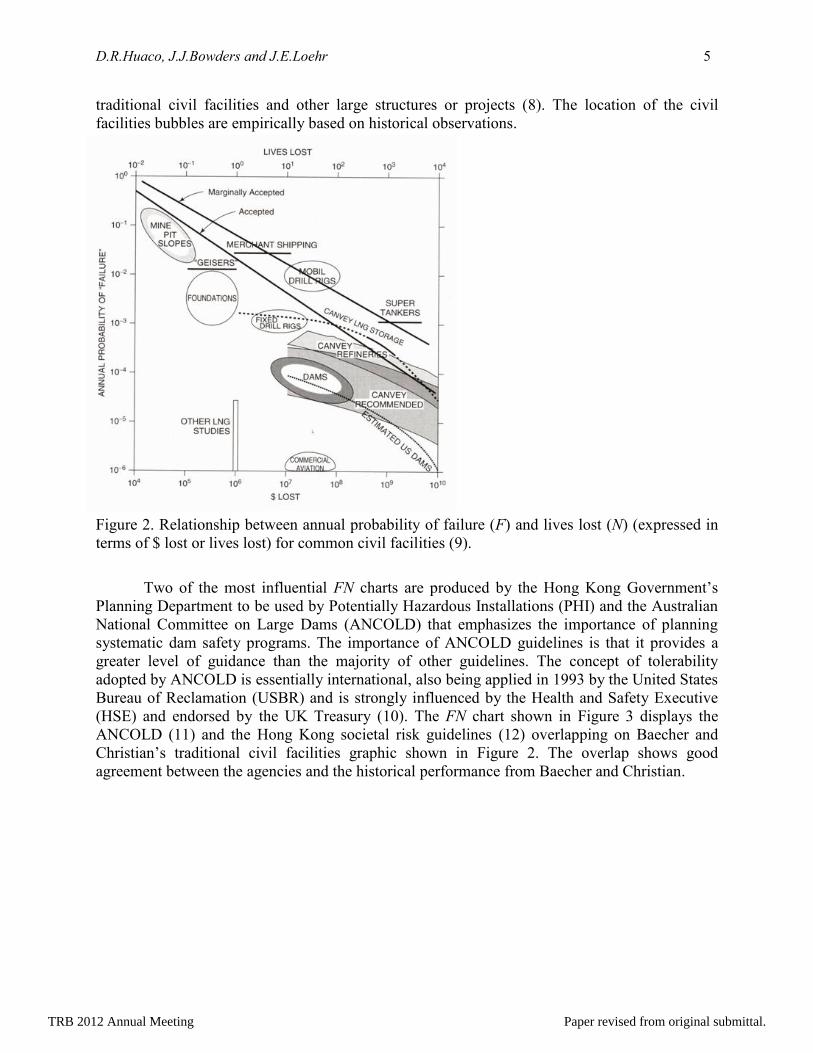
Figure 2 shows a graphic that is commonly presented to demonstrate what many people

consider to be “acceptable risk” associated with several different activities or industries. The

chart provides some general guidance on the accepted average annual risk posed by a variety of

10-0

10-1

10-2

Societal

10-3

10-4

10-5

10-6

10-7

10 102

103

104

105

106

Number of Fatalities, N

Economical

An

nu

al P

rob

ab

ility

of

"Failu

re"



traditional civil facilities and other large structures or projects (8). The location of the civil

facilities bubbles are empirically based on historical observations.

Figure 2. Relationship between annual probability of failure (F) and lives lost (N) (expressed in

terms of $ lost or lives lost) for common civil facilities (9).

Two of the most influential FN charts are produced by the Hong Kong Government’s

Planning Department to be used by Potentially Hazardous Installations (PHI) and the Australian

National Committee on Large Dams (ANCOLD) that emphasizes the importance of planning

systematic dam safety programs. The importance of ANCOLD guidelines is that it provides a

greater level of guidance than the majority of other guidelines. The concept of tolerability

adopted by ANCOLD is essentially international, also being applied in 1993 by the United States

Bureau of Reclamation (USBR) and is strongly influenced by the Health and Safety Executive

(HSE) and endorsed by the UK Treasury (10). The FN chart shown in Figure 3 displays the

ANCOLD (11) and the Hong Kong societal risk guidelines (12) overlapping on Baecher and

Christian’s traditional civil facilities graphic shown in Figure 2. The overlap shows good

agreement between the agencies and the historical performance from Baecher and Christian.



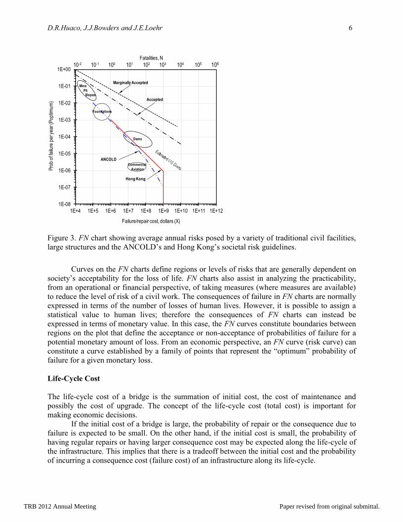
Figure 3. FN chart showing average annual risks posed by a variety of traditional civil facilities,

large structures and the ANCOLD’s and Hong Kong’s societal risk guidelines.

Curves on the FN charts define regions or levels of risks that are generally dependent on

society’s acceptability for the loss of life. FN charts also assist in analyzing the practicability,

from an operational or financial perspective, of taking measures (where measures are available)

to reduce the level of risk of a civil work. The consequences of failure in FN charts are normally

expressed in terms of the number of losses of human lives. However, it is possible to assign a

statistical value to human lives; therefore the consequences of FN charts can instead be

expressed in terms of monetary value. In this case, the FN curves constitute boundaries between

regions on the plot that define the acceptance or non-acceptance of probabilities of failure for a

potential monetary amount of loss. From an economic perspective, an FN curve (risk curve) can

constitute a curve established by a family of points that represent the “optimum” probability of

failure for a given monetary loss.

Life-Cycle Cost

The life-cycle cost of a bridge is the summation of initial cost, the cost of maintenance and

possibly the cost of upgrade. The concept of the life-cycle cost (total cost) is important for

making economic decisions.

If the initial cost of a bridge is large, the probability of repair or the consequence due to

failure is expected to be small. On the other hand, if the initial cost is small, the probability of

having regular repairs or having larger consequence cost may be expected along the life-cycle of

the infrastructure. This implies that there is a tradeoff between the initial cost and the probability

of incurring a consequence cost (failure cost) of an infrastructure along its life-cycle.

1E-08

1E-07

1E-06

1E-05

1E-04

1E-03

1E-02

1E-01

1E+00

1E+4 1E+5 1E+6 1E+7 1E+8 1E+9 1E+10 1E+11 1E+12

Pro

b o

f fa

ilure

pe

r ye

ar (

Po

ptim

um

)

Failure/repair cost, dollars (X)

Fatalities, N10-2 10-1 100 10+1 10+2 10+3 10+4 10+5 10+6

Foundations

Dams

Commercial

Aviation

Mine

PitSlopes

Marginally Accepted

Accepted

ANCOLD

Hong Kong

1E-08

1E-07

1E-06

1E-05

1E-04

1E-03

1E-02

1E-01

1E+00

1E+4 1E+5 1E+6 1E+7 1E+8 1E+9 1E+10 1E+11 1E+12

Pro

b o

f fa

ilure

pe

r ye

ar (

Po

ptim

um

)


Fatalities, N

10-2 10-1 100 101 102 103 104 105 106

Foundations

Dams

Commercial

Aviation

Mine

PitSlopes

Marginally Accepted

Accepted

ANCOLD

Hong Kong



Substructures and foundations constitute major components of bridges, and can represent

more than half of the total bridge cost (13). The method of analysis and design is important

because it can influence the structural performance and project budget.

Expected Monetary Value

In decision theory, the expected monetary value, EMV (also denoted as E), is a measure of the

value or utility expected to result from a given strategy (decision), equal to the sum of the initial

investment (cost) of a civil work plus the probability of an incurrence times the value of the

consequence (gain or loss). In the case of civil works, consequences can be classified as

recurring maintenance costs (vegetation control, drainage maintenance, etc) or unexpected

maintenance cost (repair of slides, settlement or total failure and complete replacement, etc.).

The term “consequence” is used as the costs associated with a future failure. In general,

consequence can include human injuries or other less tangible things like legal liability or

political consequences such as the loss of faith by the traveling public. In this paper,

consequences are expressed in terms of dollars to make the evaluations convenient. The

mathematical expression shown in Equation 1 represents the expected monetary value (E) of a

civil work.

( ) (1)

Where,

E = expected monetary value

A = initial cost of the civil work

P = the probability of failure

X = consequence cost of failure

T = the cost associated with no failure or recurring maintenance cost.

Since geotechnical infrastructures involve piles, drilled shafts, etc. which does not

typically require recurring maintenance, the cost of maintenance, T in the equation is considered

negligible. The simplified mathematical expression to denote the expected monetary value is

displayed as Equation 2.

(2)

The expected monetary value is now an equation with three independent variables (A, P

and X). The initial cost (A) and the probability of failure (P) are inversely related, meaning that if

the initial cost increases, it is assumed that the probability of failure decreases or if the initial cost

decreases, the probability of failure increases. In the case of geotechnical infrastructures, if the

foundation increases in cost due to an increase in size, the probability of poor performance

(settlement or collapse) is assumed to decrease.

The relations or functions between the initial costs of the geotechnical infrastructure and

the probability of failure are shown in a future section. The function that relates the initial cost, A

with the probability of failure is of the form displayed in Equation 3.

( ) (3)



Where,

A = the initial cost of the foundation,

b = the slope factor,

P = the probability of failure, and

d = the vertical intercept at P = 1.0

The values of variables b and d are obtained through probabilistic analyses and are

considered unique and constants for each type of geotechnical infrastructure. Therefore, the

expected monetary value equation is reduced to be a function of the probability, P the

consequence cost, X and a couple of known constants.

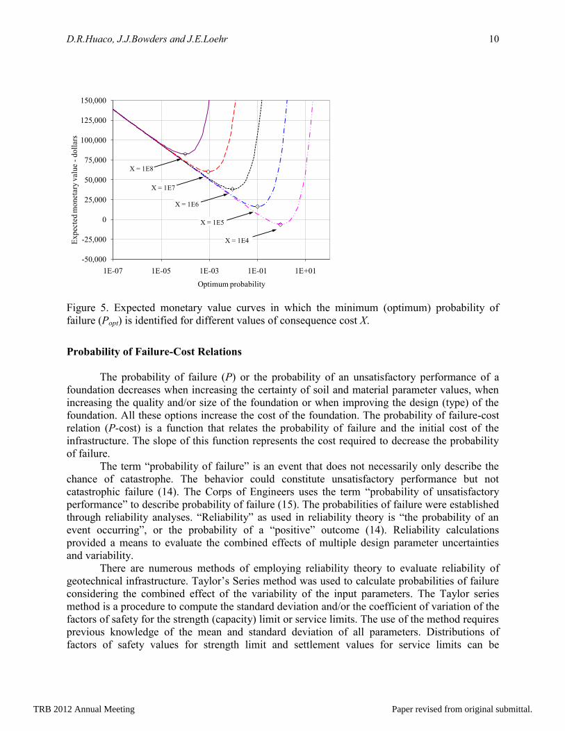
Minimum Expected Value

By relating the initial cost (A) and the probability of failure (P), the expected monetary value is

simplified to an equation of two variables. This function represents a surface in space in which

the axes are the expected monetary value (E), the probability of failure (P) and the consequence

cost (X). The surface has the shape of an open parabolic channel that flows upwards and out of

the E-P plane (Figure 4).

Figure 4 Graphical representation of the relation between the expected monetary value (E), the

probability of failure (P) and the consequence cost (X).

An upwards parabolic curve is observed on any plane parallel to the E-P plane that

intersects the X axis. By definition, this parabolic curve has a “vertex” or a point that is a

minimum on that plane. This point represents the minimum expected value (less expensive life-

cycle cost of an infrastructure) for a selected value of X. The coordinates of the minimum point

are calculated in the next section.

P

X

E



Derivation of the Optimum Probability Function and FN Curve

In Figure 4, the curve that results from intersecting the E-P-X surface with a plane parallel to the

E-P plane has a point that is a minimum (minimum expected value). The abscissa of the point is

P and the ordinate is E. The coordinates of the minimum point are calculated by mathematically

minimizing the function that defines E. The abscissa P of the minimum point is denoted as the

optimum probability (Popt) because at that value, the expected value (E) is a minimum.

From Equation 2, the value of the initial cost (A) is replaced by the function of (A) shown in

Equation 3. The expected monetary equation now has the following form (Equation 4):

( ) (4)

The minimum value of this equation occurs when its tangent (slope) is zero. This can be

calculated by taking the derivative of the expected monetary value (E) with respect to the

probability of failure (P).

The probability (P) at which the expected monetary value is minimum is defined as the optimum

probability of failure (Popt) and is denoted as follows (Equation 5).

(5)

The value of the optimum probability (Popt) will be different for different expected

monetary value curves which are generated by assigning different values to the consequence (X)

(Figure 5). It is possible to use different values of consequence because the expected monetary

value of the geotechnical infrastructure (bridge foundation) includes as a consequence, the cost

of failure of the entire bridge (X). Although the initial cost is related to the foundation only, the

consequence depends on the cost or repair of the entire bridge.

The target level of risk is plotted in an FN chart. The level of risk is plotted as a

continuous curve that is generated by a family of points that represent the optimum probabilities

of failure (Popt) of an infrastructure for different consequences (X).



Figure 5. Expected monetary value curves in which the minimum (optimum) probability of

failure (Popt) is identified for different values of consequence cost X.

Probability of Failure-Cost Relations

The probability of failure (P) or the probability of an unsatisfactory performance of a

foundation decreases when increasing the certainty of soil and material parameter values, when

increasing the quality and/or size of the foundation or when improving the design (type) of the

foundation. All these options increase the cost of the foundation. The probability of failure-cost

relation (P-cost) is a function that relates the probability of failure and the initial cost of the

infrastructure. The slope of this function represents the cost required to decrease the probability

of failure.

The term “probability of failure” is an event that does not necessarily only describe the

chance of catastrophe. The behavior could constitute unsatisfactory performance but not

catastrophic failure (14). The Corps of Engineers uses the term “probability of unsatisfactory

performance” to describe probability of failure (15). The probabilities of failure were established

through reliability analyses. “Reliability” as used in reliability theory is “the probability of an

event occurring”, or the probability of a “positive” outcome (14). Reliability calculations

provided a means to evaluate the combined effects of multiple design parameter uncertainties

and variability.

There are numerous methods of employing reliability theory to evaluate reliability of

geotechnical infrastructure. Taylor’s Series method was used to calculate probabilities of failure

considering the combined effect of the variability of the input parameters. The Taylor series

method is a procedure to compute the standard deviation and/or the coefficient of variation of the

factors of safety for the strength (capacity) limit or service limits. The use of the method requires

previous knowledge of the mean and standard deviation of all parameters. Distributions of

factors of safety values for strength limit and settlement values for service limits can be

-50,000

-25,000

0

25,000

50,000

75,000

100,000

125,000

150,000

1E-07 1E-05 1E-03 1E-01 1E+01

Ex

pec

ted

mo

net

ary

val

ue

-d

oll

ars

Optimum probability

X = 1E8

X = 1E7

X = 1E6

X = 1E5

X = 1E4



developed using the mean and standard deviations values computed using Taylor’s Series

method.

Distributions of factors of safety values for bridge foundation strength and service limits

are assumed to be lognormal. The magnitude of the probability of failure is established by

computing the area under the distribution curve less than unity (1.0) and the probability of

exceeding a selected service limit was established by computing the area under the settlement

value distribution curve larger than the select service limit. The initial cost, A of foundations

depends of the foundation type, size and the cost of materials.

Probabilities of failure-cost curves are developed by plotting the probability and cost

pairs on semi-log graphs. Probability values are plotted in a log scale while the costs are plotted

on an arithmetic scale. The probabilities of failure-cost functions can be established using

regression analysis considering a logarithmic regression type. The functions that best fit the data

and can predict values of probability of failure and costs are displayed on the graphs.

The function reported has a linear form with the independent parameter, probability of

failure (abscissa), expressed in a natural log scale instead of a logarithmic scale (to base 10). The

independent constant, (d) which is an arithmetic value, represents the intersection of the function

curve with a vertical line that passes through the probability of failure value equal to unity (P =

1.0). The term with the independent variable (probability of failure, P) is affected in Equation 3

by a factor (b) which is not the true slope (m) of the linear function. The factor b is acting on the

natural log value of the probability of failure instead of the logarithmic value of the probability

of failure on a semi log graph.

The value of the slope factor b can be expressed in terms of the true function slope, m.

Consider the following linear equation in a semi log graph (Equation 6):

( ) (6)

Where,

A = the foundation initial cost,

m = the slope of the linear function,

P = the probability of failure, and

d = the vertical intercept at P = 1.0

A relation between the slope factor b and the slope m is established by comparing the terms with

the independent variable P of Equation 3 and Equation 6. The relation between the slope factor b

and the slope m is shown in Equation 7.

( ) (7)

Therefore quantitatively, the value of the slope factor b is about 40 percent of the value of

the true slope of the probability of failure-cost function in a semi-log plane. The optimum

economic probability of failure can be expressed in terms of slope factor b or in terms of the true

slope m of the function.



The location of the risk curves in the FN chart depends of the value of the slope factor b

which is obtained from the probability of failure-cost function. The slope factor b of the

probability of failure-cost function is an essential parameter to define, understand and compare

functions. This factor represents the cost required to decrease the probability of failure of a

bridge foundation by one order of magnitude. A large slope factor b would indicate that it is very

expensive to decrease the probability of failure by one order of magnitude. The locations of these

risk curves in the FN charts are evaluated with respect to their proximity to socially acceptable

risk boundaries and regions.

Development, Analysis and Calibration of Risk Curves

FN charts are graphical representations of social acceptability for the loss of lives. The risk

curves proposed by world government safety agencies on FN charts are boundaries that define

regions or levels of risk acceptable to society. They are not curves that define the economically

optimum acceptable risk. However, it is in this chart of regions of social acceptability that the

optimum economical risk curves are plotted. The optimal economic risk curves do not define

regions of economic acceptability. These curves represent a family of points of probabilities that

are economically optimum for different levels of consequence. Considering that economic risk

curves are dependent on the same parameters as socially acceptable risk (i.e. consequence (X)

and probability of failure (P)), they can be plotted on FN charts overlapping socially acceptable

regions.

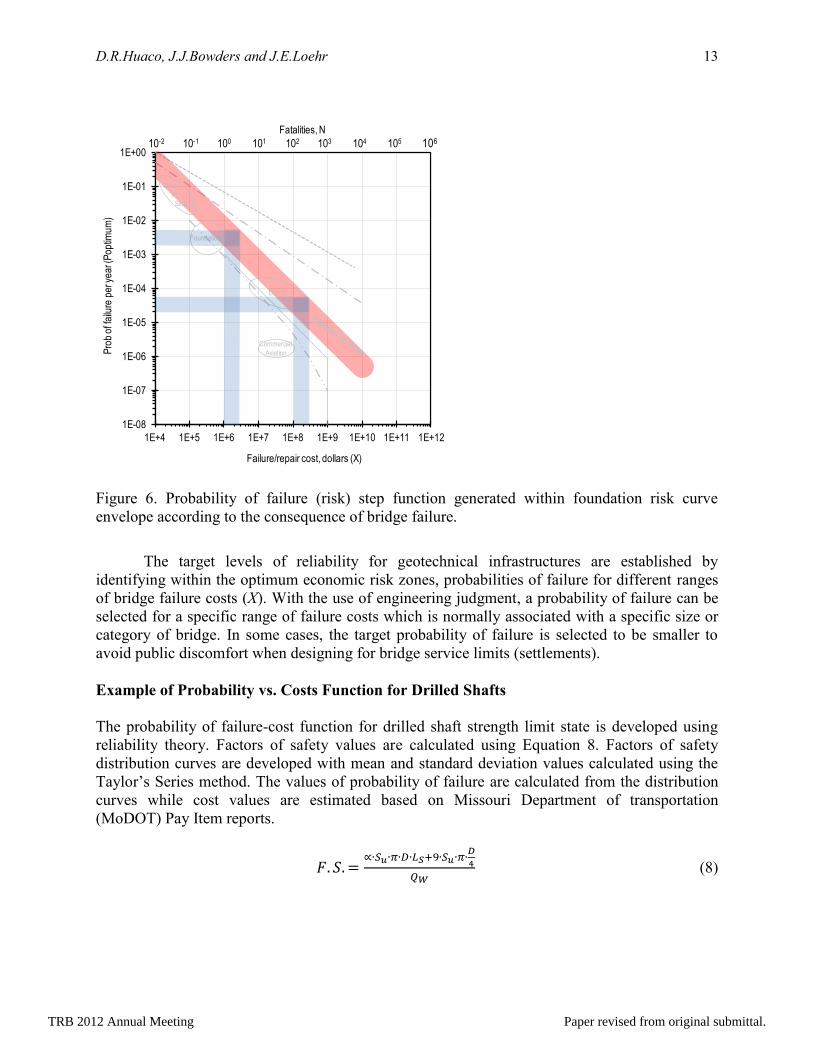
Optimum economic risk curves can be developed for several bridge foundations types

such as pile groups, drilled shafts and spread footings. The region in the FN chart that occupies

the envelope of the curves constitutes an optimum economic zone. It is within the region that the

optimum probabilities of failure are established. Figure 6 shows the shaded region of an

optimum economic risk curve envelope developed for the design of bridge foundations

considering the strength limit.



Figure 6. Probability of failure (risk) step function generated within foundation risk curve

envelope according to the consequence of bridge failure.

The target levels of reliability for geotechnical infrastructures are established by

identifying within the optimum economic risk zones, probabilities of failure for different ranges

of bridge failure costs (X). With the use of engineering judgment, a probability of failure can be

selected for a specific range of failure costs which is normally associated with a specific size or

category of bridge. In some cases, the target probability of failure is selected to be smaller to

avoid public discomfort when designing for bridge service limits (settlements).

Example of Probability vs. Costs Function for Drilled Shafts

The probability of failure-cost function for drilled shaft strength limit state is developed using

reliability theory. Factors of safety values are calculated using Equation 8. Factors of safety

distribution curves are developed with mean and standard deviation values calculated using the

Taylor’s Series method. The values of probability of failure are calculated from the distribution

curves while cost values are estimated based on Missouri Department of transportation

(MoDOT) Pay Item reports.

(8)

1E-08

1E-07

1E-06

1E-05

1E-04

1E-03

1E-02

1E-01

1E+00

1E+4 1E+5 1E+6 1E+7 1E+8 1E+9 1E+10 1E+11 1E+12

Pro

b o

f fa

ilure

pe

r ye

ar (

Po

ptim

um

)


Foundations

Commercial

Aviation

Estimated US Dams

Dams

Mine

PitSlopes

Fatalities, N

10-2 10-1 100 101 102 103 104 105 106



Where,

F.S. = the factor of safety

α = skin resistance coefficient

Su = undrained shear strength

D = drilled shaft diameter

LS = drilled shaft length

Qw = working load.

A factor of safety distribution curve is developed for several drilled shaft sizes. Each

factor of safety distribution curve generates a probability of failure data point. Depending on the

size, each drilled shaft is also associated with a cost. Pairs of probability of failure and cost are

plotted on a semi-log graph as shown in Figure 7.

Figure 7. Probability of failure-cost function for drilled shafts.

Using Excel’s regression functions, a logarithmic type trend line for the probability of

failure-cost points are generated. The interval of interest ranges between 1 in a hundred (1x10-2

)

and 1 in a million (1x10-6

) probability of failure. The slope factor b of the function is -17,067.

The negative sign denotes an inverse correlation. The probability of failure decreases as the costs

increases.

Similarly, a probability of failure-cost function is developed for a pile group limit state

using Equation 9.

(9)

Where,

F.S. = the factor of safety

Fy = the pile yield strength

y = -17,067ln(x) - 12,615

0

10,000

20,000

30,000

40,000

50,000

60,000

70,000

80,000

90,000

100,000

1E-06 1E-05 1E-04 1E-03 1E-02 1E-01 1E+00

Dril

led

sh

aft

cost

, d

olla

rs,

(A)

Probability of failure, (P)



A = Cross sectional area of pile

n = number of piles in the pile group, and

Qw = working load.

The probability of failure-cost function generated for pile group strength is shown in Figure 8.

The slope factor b of the function is -1,352. Both drilled shafts and pile group risk curves fall

within the region of social acceptability for civil works. This slope is smaller in magnitude than

the slope generated for drilled shaft (b = -17,067). Risk curves of drilled shafts are located at

higher risk levels than pile group risk curves. Drilled shafts slope factors b are larger in

magnitude than pile group factors therefore it is more costly to decrease the probability of failure

of drilled shafts. The target level of probability of failure for the design of drilled shafts from an

economic perspective is larger than for pile groups.

Figure 8. Probability of failure-initial cost function for pile groups.

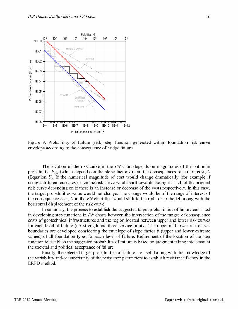
Risk curves are developed using both drilled shafts and pile group slope factors (Figure

9). The target levels of reliability for bridge foundations are established by identifying within the

area between both risk curves, the probabilities of failure for different bridge failure costs values

X.

With the use of engineering judgment a probability of failure is selected for a specific

range of failure cost that can be associated with size or category of a bridge. Graphically, the

selection of consequence costs and target probabilities appear as step functions within the

optimum economic risk zone.

A = -1,352 ln(P) + 17,043

0

5,000

10,000

15,000

20,000

25,000

30,000

35,000

1E-08 1E-07 1E-06 1E-05 1E-04 1E-03 1E-02 1E-01 1E+00

Co

st p

ile g

rou

p, 5

0 f

t lo

ng

, d

olla

rs,

(A)

Probability of elastic failure, (P)



Figure 9. Probability of failure (risk) step function generated within foundation risk curve

envelope according to the consequence of bridge failure.

The location of the risk curve in the FN chart depends on magnitudes of the optimum

probability, Popt (which depends on the slope factor b) and the consequences of failure cost, X

(Equation 5). If the numerical magnitude of cost would change dramatically (for example if

using a different currency), then the risk curve would shift towards the right or left of the original

risk curve depending on if there is an increase or decrease of the costs respectively. In this case,

the target probabilities value would not change. The change would be of the range of interest of

the consequence cost, X in the FN chart that would shift to the right or to the left along with the

horizontal displacement of the risk curve.

In summary, the process to establish the suggested target probabilities of failure consisted

in developing step functions in FN charts between the intersection of the ranges of consequence

costs of geotechnical infrastructures and the region located between upper and lower risk curves

for each level of failure (i.e. strength and three service limits). The upper and lower risk curves

boundaries are developed considering the envelope of slope factor b (upper and lower extreme

values) of all foundation types for each level of failure. Refinement of the location of the step

function to establish the suggested probability of failure is based on judgment taking into account

the societal and political acceptance of failure.

Finally, the selected target probabilities of failure are useful along with the knowledge of

the variability and/or uncertainty of the resistance parameters to establish resistance factors in the

LRFD method.

1E-08

1E-07

1E-06

1E-05

1E-04

1E-03

1E-02

1E-01

1E+00

1E+4 1E+5 1E+6 1E+7 1E+8 1E+9 1E+10 1E+11 1E+12

Pro

b o

f fa

ilure

pe

r ye

ar (

Po

ptim

um

)


Foundations

Dams

Commercial

Aviation

Mine

PitSlopes

Marginally Accepted

Accepted

ANCOLD

Hong Kong

1E-08

1E-07

1E-06

1E-05

1E-04

1E-03

1E-02

1E-01

1E+00

1E+4 1E+5 1E+6 1E+7 1E+8 1E+9 1E+10 1E+11 1E+12

Pro

b o

f fa

ilure

pe

r ye

ar (

Po

ptim

um

)


Foundations

Dams

Commercial

Aviation

Mine

PitSlopes

Marginally Accepted

Accepted

ANCOLD

Hong Kong

Fatalities, N

10-2 10-1 100 101 102 103 104 105 106



CONCLUSIONS

Target levels of reliability for the design of geotechnical infrastructures can be established based

on a combination of cost analysis and societal acceptance of risk. The levels of reliability

obtained from the optimization of cost and risk provides the opportunity to decrease the costs of

an infrastructure while designing to a consistent known level of safety. The engineering

procedure is robust and can be applied to develop target levels of reliability for other civil works.

ACKNOWLEDGEMENTS

The authors of this paper would like to thank the Missouri Department of Transportation

(MoDOT) for providing funding and information for the project. We would also like to thank Dr.

Carmen Chicone, professor of the Department of Mathematics of the University of Missouri for

his invaluable contributions and recommendations to this project.

REFERENCES

1. Orr, T. L. (2005). “Proceedings of the International Workshop on the Evaluation of

Eurocode 7”. ERTC 10 of the International Society for Soil Mechanics and Geotechnical

Engineering and Department of Civil, Structural and Environmental Engineering, Trinity

College, Dublin. March 31 and April 1, 2005.

2. Kulicki, J.M., Prucz, Z., Clancy, C.M., Mertz, D.R., Nowak, A.S. (2007). Updating the

Calibration Report for AASHTO LRFD Code. Final Report. Project No. NCHRP 20-7/186.

National Cooperative Highway Research Program. Transportation Research Board (TRB).

3. Chang, Nien-Yin. (2006). Report No. CDOT-DTD-R-2006-7. CDOT Foundation Design

Practice and LRFD Strategic Plan. Colorado Department of transportation – Reseach

Branch. February 2006.

4. AASHTO (2004). AASHTO LRFD Bridge Design Specifications, Customary U.S. units,

Third edition, 2004, American Association of State Highway & Transportation Officials.

5. KDOT (2008). Kansas Department of Transportation Design Manual. Bridge Section,

Volume III (LRFD). Version 9/08

6. Ball, D.J., Floyd, P.J. (1998). “Societal Risks”, Final Report. Report Commissioned by the

Health and Safety Executive, United Kingdom.

7. Evans, A.W., (2003). Transport Fatal Accidents and FN Curves 1967-2001. Research

Report 073. HSE Books, ISBN 0 7176 2623 7.

8. Baecher, G.B. (1982a). Simplified Geotechnical Data Analysis, Reliability Theory and Its

Application in Structural and Soil Engineering. The Hague: Martinus Nijhoff Publishers.

9. Baecher, G.B., J.T. Christian (2003). Reliability and Statistics in Geotechnical Engineering,

Chichester, England ; Hoboken, NJ : Wiley.

10. HM Treasury United Kingdom (1996). The Setting of Safety Standards, a report by an

interdepartamental group and esternal advisers, June.

11. ANCOLD (1994). "Guidelines on Risk Assessment 1994." Australia-New Zealand

Committee on Large Dams. Guidelines on Dam Safety Management.



12. Hong Kong Government Planning Department (1994). "Hong Kong Planning Standards

and Guidelines, Chapter 11, Potentially Hazardous Installations." Hong Kong.

13. Xanthakos, P.P. (1996). Bridge Substructure and Foundation Design. Prentice Hall. 1st

edition. ISBN-10: 0-13-300617-4. ISBN-13: 978-0-13-300617-9

14. Duncan, J.M., Navin, M., Patterson, K. (1999). Manual for Geotechnical Engineering

Reliability Calculations. Virginia Polytechnic Institute and State University.

15. U.S. Army Corps of Engineers (1998). “Risk Based Analysis in Geotechnical Engineering

for Support of Planning Studies,” Engineering Circular No. 1110-2-554, Department of the

Army U.S. Army Corps of Engineers, Washington D.C., 27 February 1998. (Available

online at www.usace.army.mil/usace-docs).


Documents

Method to Develop Target Levels of Reliability for Design Using LRFD