International Archives of Photogrammetry and Remote Sensing. Vol. XXXII, Part 5. Hakodate 1998

Method of sequential image analysis with telescopic pole for traffic flow measurement

Hiroshi TAKEDA, Masahiro SETOJIMA, Naruo MUSHIAKE Image Analysis Section Engineer, Department of Emviroment

KOKUSAI KOGYO Co., LTD Yoshiaki YOSHINO, Jinkei TAMADA

Ministry of Construction 5 Sanban-cho, Chiyoda-ku, Tokyo, 102-0075

JAPAN

Commission V, Working Group IC V/111

1. Introduction An increasing number of traffic flow

measurement systems equipped with video cameras are being used.1> 2> These measurement systems are used to determine the number of vehicles, vehicle velocity, and vehicle type. Most of these traffic flow measurement cameras are stationary, installed along expressways and major highways.3> Because of economical and locational conditions, installation of stationary cameras along general roads is difficult in many cases.

In this study, portable telescopic poles were used for observation and measurement of traffic flow on general roads. Cameras mounted on telescopic poles used in the study could be extended up to 20m for observation. This permitted observation measurements to be taken from viewpoints higher than ordinary stationary cameras. In addition, the use of telescopic pole cameras offered high-precision measurement by allowing points directly under the camera to be recorded.

In the study, the speed, length and number of test vehicles passing through a linear section of a general highway were measured by spatio­temporal image analysis. The study was conducted in order to examine the possibility of determining vehicle type on the basis of the measured vehicle length. Loci of traveling vehicles were also measured in a test road section modeled after an intersection.

2. Equipment Observation of general roads other than

expressways and major highways may need multiple observation points, so installation of stationary cameras will be difficult. The installation height of ordinary stationary cameras is low. As a result, the observation angle with respect to the ground is less, reducing the

814

measurement accuracy of spatial depth, when it is intended to ensure a wide observation area.

In this study, telescopic poles (Fig.1) were used as observation platforms. The main focuses of the observation were to stress the importance of the mobility of these poles and the stability of the video cameras, when taking measurements from an elevated position during the observations. These motor-driven telescopic poles can extend from 3 m to 15 m above ground. The telescopic pole is mounted on a caterpillar, which permits the telescopic pole to be moved over short distances. In addition, because the telescopic poles may be loaded onto trucks, they can be transported over long distances.

Use of telescopic poles ensures stable images observed from a high view point and may even be used on general roads in areas where there are no high-rise buildings on which to mount cameras. Table 1 shows specifications for equipment of telescopic poles.

1 bl 1 S "f f a e pecI Icat1ons or equipment item spec

(1) body max. length 19.84m min. length 2.95m pole diameter 280mm motor box size 410x563mm weight 185kg material Carbon FRP permitted weight 10kg expansion speed 1.7m/min.

(2) video camera body size 70x72x124mm weight 0.67kg focus of lens 7.5-90mm iris F1.4-F16 CCD type interlace 112inch

(a) When retracted (b) When extended Fig.1 Appearance of telescopic pole

3. Test method 3.1 Linear section of general road

Telescopic poles were installed on one side of a general road for continuous observation for approx. 1 hour. Three test vehicles dispersed among ordinary vehicles traveled under the following conditions:

~ A single lane road was selected for traffic flow measurement

~ Telescopic poles were installed at points approx. 1 Om away from the center of the road and were extended up to a height of approx. 20m.

~ Two compact car, one white and one black, and a large-sized yellow car, were used as test vehicles.

~ The test vehicles traveled at a constant velocity in the test section.

~ The velocity was set in four patterns at 15, 30 45 and 60 km/h, and the test was repeat~d 6 times, respectively.

~ The velocity obtained by measuring the time necessary for the test vehicles to pass through the specified section (25 m) was used as verification data.

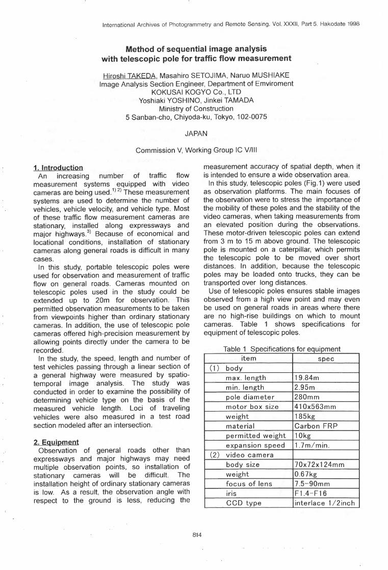
Fig.2 shows an example of the image ~f an observed test vehicle traveling through the linear section of general road.

815

Fig.2 Image observed in linear section

3.2 Traveling locus test section Assuming the observation of traveling loci of

vehicles at intersections, a test was conducted on a site other than a public road in order to measure the traveling loci of vehicles under the following conditions:

~ A telescopic pole was installed at a location approx. 15m away from the center of the observation range, and was extended up to a height of approx. 15m.

~ Traveling reference lines of 5, 10, and 15m in radius were marked on the road surface.

~ A white and a black compact car were used as test vehicles.

~ The test vehicles drove with their right-side tires along the traveling reference lines.

~ The two test vehicles, traveling first at a constant velocity and then traveling with an approx. 2-second stoppage, were observed 5 times, respectively.

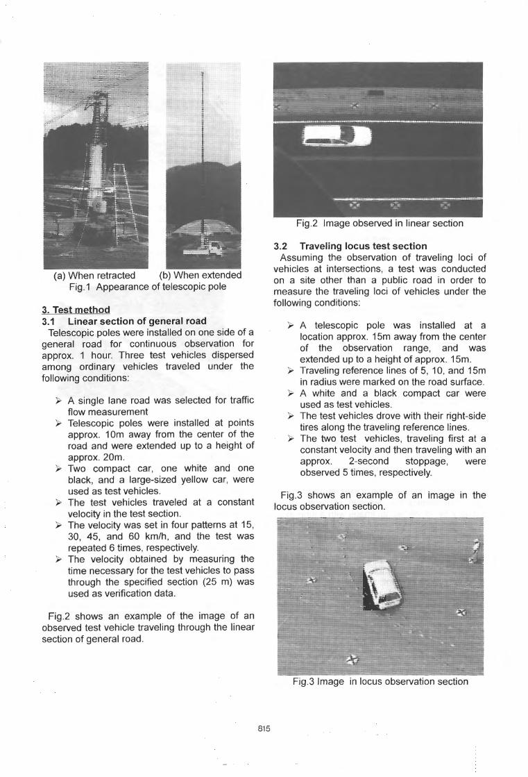
Fig.3 shows an example of an image in the locus observation section.

Fig.3 Image in locus observation section

4. Method of analysis 4.1 Flow of analysis

In the study, the method of measurement was classified according purpose. The test was classified into cases where the traveling locus was known and where the traveling locus was to be measured.

In the former case, a test was conducted in a linear section of general road in order to measure the speed, length, and number of vehicles passing through a predetermined section. In the latter case, vehicle traveling loci (two-dimensional behavior of vehicles) were measured.Fig.4 shows the flow of analysis.

lnprt Sequmtial Image

Making of ~ Slit Image

ExtractofVehideR,gioo

Mmun,mmtofSlq,eaod\\idlh on~Slitlmage

Reiults of Speed, ungdi and Amount of Vehicles

Making of lnlfr-frame llffermtial Image

ExtractofVehideR,gioo

Q-avityofVehide ReiultsofVehidelorus

Fig.4 Flow of analysis

4.2 Spatio-temporal image processing By representing the direction of depth of an

ordinary two-dimensional image with a time axis, a three-dimensional image is created. This image is called a spatio-temporal image.

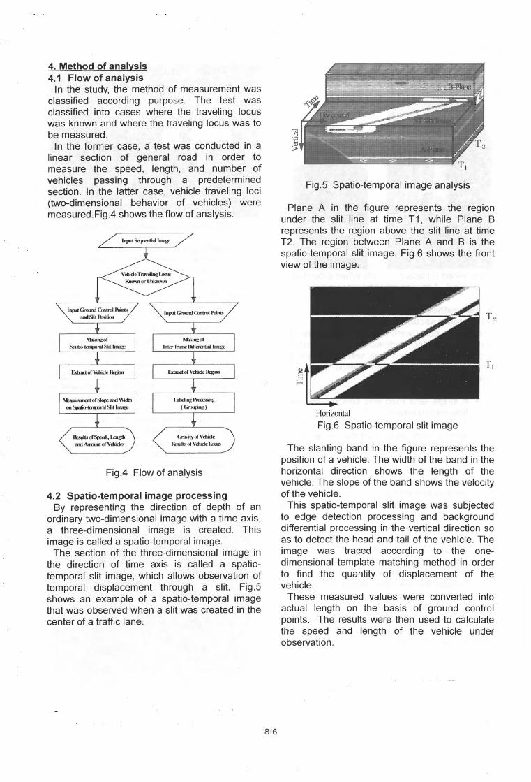
The section of the three-dimensional image in the direction of time axis is called a spatio­temporal slit image, which allows observation of temporal displacement through a slit. Fig.5 shows an example of a spatio-temporal image that was observed when a slit was created in the center of a traffic lane.

816

Fig.5 Spatio-temporal image analysis

Plane A in the figure represents the region under the slit line at time T1, while Plane B represents the region above the slit line at time T2. The region between Plane A and B is the spatio-temporal slit image. Fig.6 shows the front view of the image.

Horizontal

Fig.6 Spatio-temporal slit image

The slanting band in the figure represents the position of a vehicle. The width of the band in the horizontal direction shows the length of the vehicle. The slope of the band shows the velocity of the vehicle.

This spatio-temporal slit image was subjected to edge detection processing and background differential processing in the vertical direction so as to detect the head and tail of the vehicle. The image was traced according to the one­dimensional template matching method in order to find the quantity of displacement of the vehicle.

These measured values were converted into actual length on the basis of ground control points. The results were then used to calculate the speed and length of the vehicle under observation.

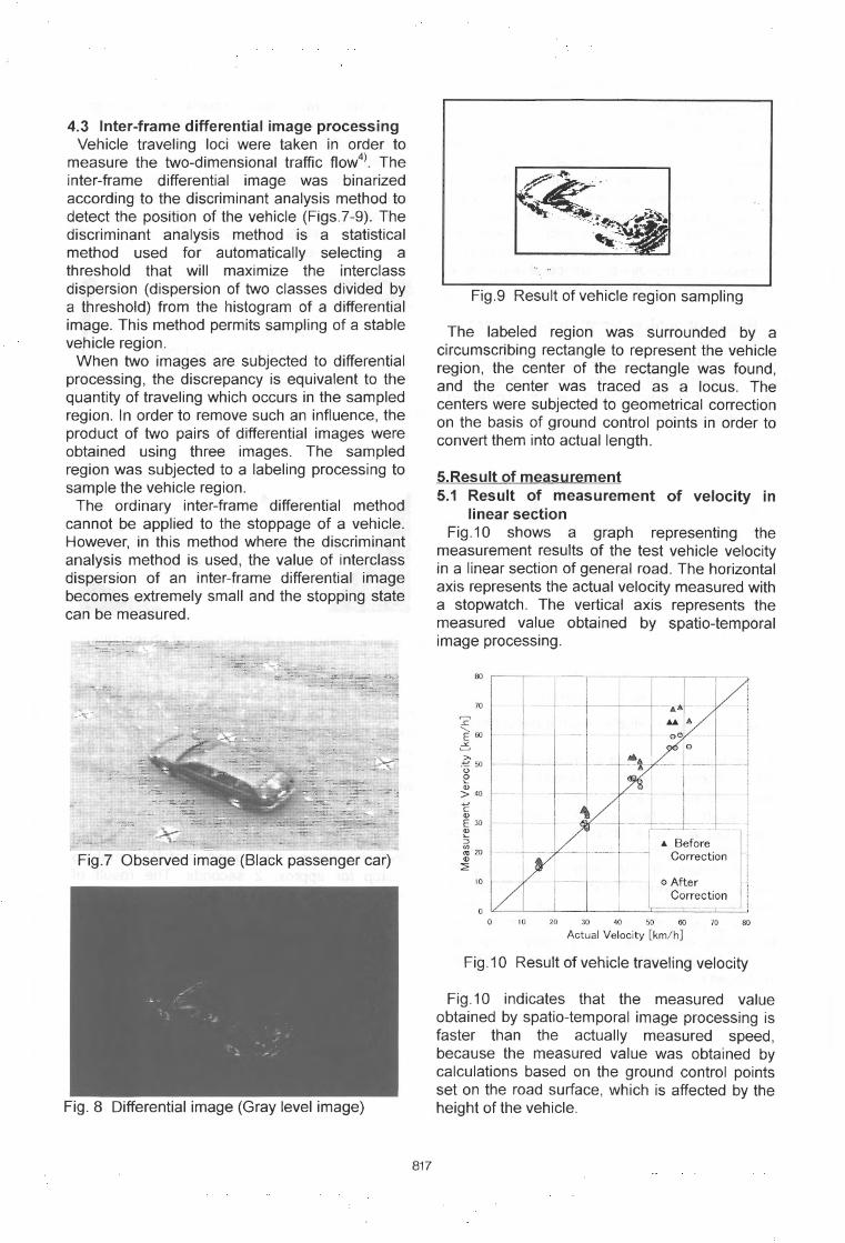
4.3 Inter-frame differential image processing Vehicle traveling loci were taken in order to

measure the two-dimensional traffic flow4>. The inter-frame differential image was binarized according to the discriminant analysis method to detect the position of the vehicle (Figs.7-9). The discriminant analysis method is a statistical method used for automatically selecting a threshold that will maximize the interclass dispersion (dispersion of two classes divided by a threshold) from the histogram of a differential image. This method permits sampling of a stable vehicle region.

When two images are subjected to differential processing, the discrepancy is equivalent to the quantity of traveling which occurs in the sampled region. In order to remove such an influence, the product of two pairs of differential images were obtained using three images. The sampled region was subjected to a labeling processing to sample the vehicle region.

The ordinary inter-frame differential method cannot be applied to the stoppage of a vehicle. However, in this method where the discriminant analysis method is used, the value of interclass dispersion of an inter-frame differential image becomes extremely small and the stopping state can be measured.

Fig. 8 Differential image (Gray level image)

817

Fig.9 Result of vehicle region sampling

The labeled region was surrounded by a circumscribing rectangle to represent the vehicle region, the center of the rectangle was found, and the center was traced as a locus. The centers were subjected to geometrical correction on the basis of ground control points in order to convert them into actual length.

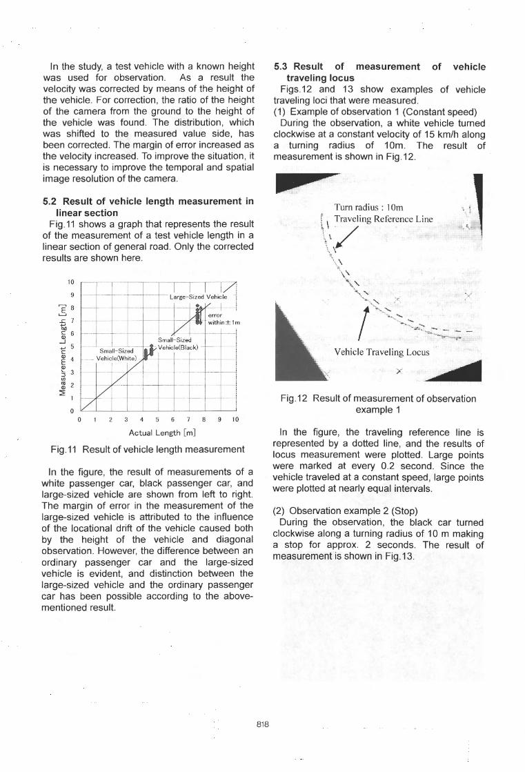
5.Result of measurement 5.1 Result of measurement of velocity in

linear section Fig.10 shows a graph representing the

measurement results of the test vehicle velocity in a linear section of general road. The horizontal axis represents the actual velocity measured with a stopwatch. The vertical axis represents the measured value obtained by spatio-temporal image processing.

70 I----+-~--+-- t--------t--

2 '­E 60 -+-------i--- -1 - ---- - - ---

6 >,

.-!:! 50 1------t-- -,-­o e ~ 40 - -+-----+- --+- --Y--- t------t--t--------i ..., C (1)

E 30

~ :::,

~ 20 l-------t--,r---~1 - -+---------1 (1)

.a. Before Correction

~

10 @ After Correction

10 20 30 40 50 60 70 80

Actual Velocity [km/h]

Fig.1 O Result of vehicle traveling velocity

Fig.1 O indicates that the measured value obtained by spatio-temporal image processing is faster than the actually measured speed, because the measured value was obtained by calculations based on the ground control points set on the road surface, which is affected by the height of the vehicle.

In the study, a test vehicle with a known height was used for observation. As a result the velocity was corrected by means of the height of the vehicle. For correction, the ratio of the height of the camera from the ground to the height of the vehicle was found. The distribution, which was shifted to the measured value side, has been corrected. The margin of error increased as the velocity increased. To improve the situation, it is necessary to improve the temporal and spatial image resolution of the camera.

5.2 Result of vehicle length measurement in linear section

Fig.11 shows a graph that represents the result of the measurement of a test vehicle length in a linear section of general road. Only the corrected results are shown here.

10

9

,......, 8 ..s ..c:: 7 to ~ 6

...J ..., 5 C:

~ 4 Q)

~ 3 (/)

:g 2

~

0

I I I I/! ~- -- -- - Large-Sized Vehicle ·1 ~ --- • V I

l,,if ' error

V .. within±1 m

-·

Small-Sized ______ ......... . _. l.f' Vehicle(Black) Small-Sized -- Vehicle(Whv

V --- -

[7 L~

0 2 3 4 5 6 7 8 9 10

Actual Length [m]

Fig.11 Result of vehicle length measurement

In the figure, the result of measurements of a white passenger car, black passenger car, and large-sized vehicle are shown from left to right. The margin of error in the measurement of the large-sized vehicle is attributed to the influence of the locational drift of the vehicle caused both by the height of the vehicle and diagonal observation. However, the difference between an ordinary passenger car and the large-sized vehicle is evident, and distinction between the large-sized vehicle and the ordinary passenger car has been possible according to the above­mentioned result.

818

5.3 Result of measurement of vehicle traveling locus

Figs.12 and 13 show examples of vehicle traveling loci that were measured. (1) Example of observation 1 (Constant speed)

During the observation, a white vehicle turned clockwise at a constant velocity of 15 km/h along a turning radius of 1 Om. The result of measurement is shown in Fig.12.

Tum radius : I Om ( \ Traveling Reference Line

\\/ \~.\

~

Vehicle Traveling Locus

x: ·~

Fig.12 Result of measurement of observation example 1

In the figure, the traveling reference line is represented by a dotted line, and the results of locus measurement were plotted. Large points were marked at every 0.2 second. Since the vehicle traveled at a constant speed, large points were plotted at nearly equal intervals.

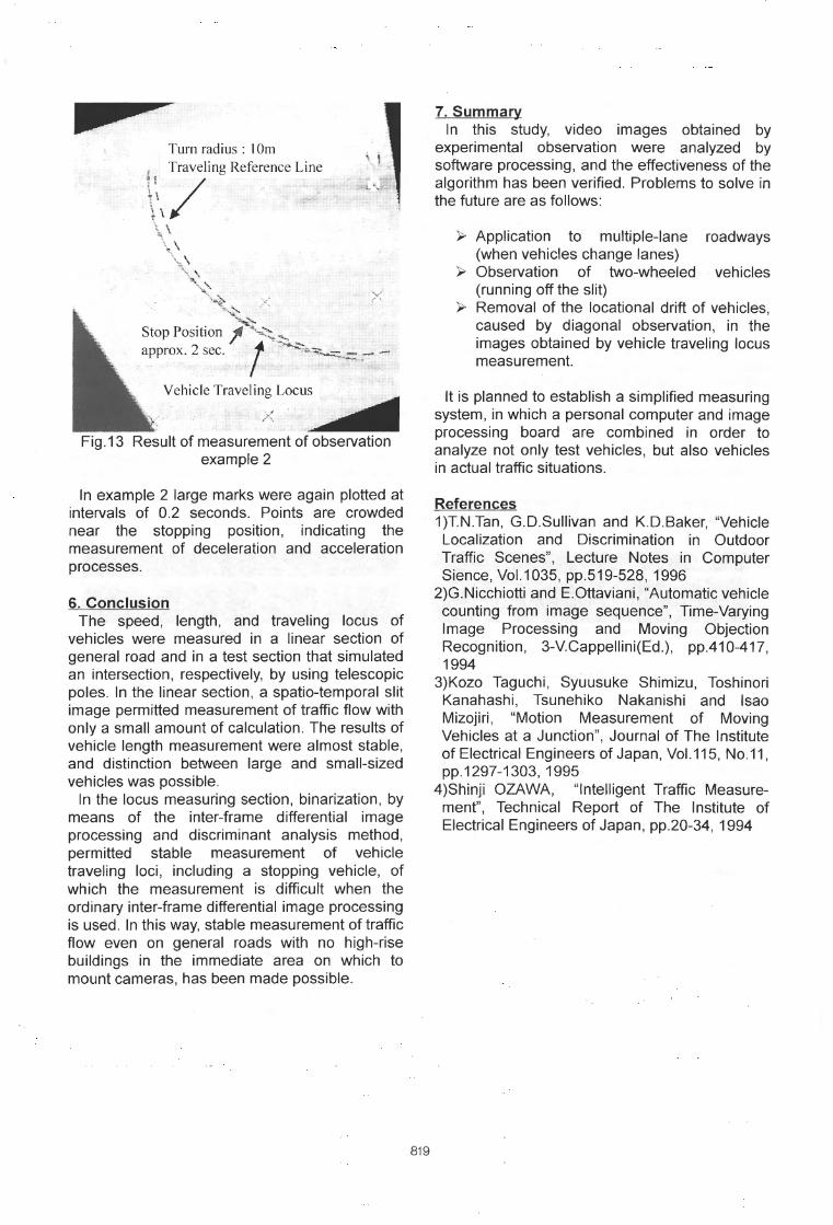
(2) Observation example 2 (Stop) During the observation, the black car turned

clockwise along a turning radius of 10 m making a stop for approx. 2 seconds. The result of measurement is shown in Fig.13.

Turn radius: I Orn

h T/raveling Reference Line

\\ . . '

\_ \ \,\ ~-\,\

'\,:, ' -,._t

v

' i . '

Stop Position ~~-' r/ ~-..., approx. 2 sec. ~~;:::-__- -

Vehicle Traveli"! Locu:............

Fig.13 Result of measurement of observation example 2

In example 2 large marks were again plotted at intervals of 0.2 seconds. Points are crowded near the stopping position, indicating the measurement of deceleration and acceleration processes.

6. Conclusion The speed, length, and traveling locus of

vehicles were measured in a linear section of general road and in a test section that simulat~d an intersection, respectively, by using telescopic poles. In the linear section, a spatio-t~mporal ~lit image permitted measurement of traffic flow with only a small amount of calculation. The results of vehicle length measurement were almost stable, and distinction between large and small-sized vehicles was possible.

In the locus measuring section, binarization, by means of the inter-frame differential image processing and discriminant analysis meth_od, permitted stable measuremen_t of _vehicle traveling loci, including a stopping vehicle, of which the measurement is difficult when the ordinary inter-frame differential image processing is used. In this way, stable measurement of traffic flow even on general roads with no high-rise buildings in the immediate area on which to mount cameras, has been made possible.

819

7. Summary In this study, video images obtained by

experimental observation were analyzed by software processing, and the effectiveness of the algorithm has been verified. Problems to solve in the future are as follows:

~ Application to multiple-lane roadways (when vehicles change lanes)

~ Observation of two-wheeled vehicles (running off the slit)

~ Removal of the locational drift of vehicles, caused by diagonal observation, in the images obtained by vehicle traveling locus measurement.

It is planned to establish a simplified measuring system, in which a personal computer and image processing board are combined in order to analyze not only test vehicles, but also vehicles in actual traffic situations.

References 1)TN.Tan, G.D.Sullivan and K.D.Baker, "Vehicle Localization and Discrimination in Outdoor Traffic Scenes", Lecture Notes in Computer Sience, Vol.1035, pp.519-528, 1996

2)G.Nicchiotti and E.Ottaviani, "Automatic vehicle counting from image sequence", Time-Varying Image Processing and Moving Objection Recognition, 3-V.Cappellini(Ed.), pp.410-417, 1994

3)Kozo Taguchi, Syuusuke Shimizu, Toshinori Kanahashi, Tsunehiko Nakanishi and lsao Mizojiri, "Motion Measurement of Moving Vehicles at a Junction", Journal of The Institute of Electrical Engineers of Japan, Vol.115, No.11, pp.1297-1303, 1995

4)Shinji OZAWA, "Intelligent Traffic Measure­ment", Technical Report of The Institute of Electrical Engineers of Japan, pp.20-34, 1994