Embed Size (px)
Citation preview

METHOD FOR RAPID ESTIMATION OF
SCOUR AT HIGHWAY BRIDGES BASED
ON LIMITED SITE DATA
By Stephen R. Holnbeck and Charles Parrett
U.S. GEOLOGICAL SURVEY
Water-Resources Investigations Report 96-4310
Prepared in cooperation with the
MONTANA DEPARTMENT OF TRANSPORTATION
Helena, Montana
March 1997

U.S. DEPARTMENT OF THE INTERIOR
BRUCE BABBITT, Secretary
U.S. GEOLOGICAL SURVEY
Gordon P. Eaton, Director
For additional information write to:
District Chief U.S. Geological Survey Federal Building, Drawer 10076 Helena, MT 59626-0076
Copies of this report may be purchased from:
U.S. Geological Survey Branch of Information Services Box 25286 Denver, CO 80225-0286

CONTENTS
Page
Abstract...................................................................................................................................................^ 1Introduction.......................................................................................................................................................................^ 3Scour at highway bridges...................................................................................................................................................... 3
Background.............................................................^ 4Description of the Level 2 analyses........................................................................................................................... 7
General considerations................................................................................................................................... 7Water-surface profile analysis........................................................................................................................ 8Scour-prediction equations............................................................................................................................. 8
Contraction scour................................................................................................................................ 8Pier scour............................................................................................................................................ 14Abutment scour................................................................................................................................... 15
Development of rapid-estimation method............................................................................................................................. 17Level 2 scour-analysis data used ............................................................................................................................... 17Variables relating to Level 2 scour depths................................................................................................................. 19
Contraction scour........................................................................................................................................... 19Pierscour..................................................................^ 31Abutment scour.............................................................................................................................................. 34
Field testing of method.............................................................................................................................................. 35Application of rapid-estimation method ............................................................................................................................... 39
Use of limited site data to estimate scour.................................................................................................................. 39Estimating important hydraulic variables ...................................................................................................... 39
100-year peak discharge ..................................................................................................................... 40Velocity............................................................................................................................................... 40Flow depths......................................................................................................................................... 42
Estimating contraction scour.......................................................................................................................... 44Live-bed scour.................................................................................................................................... 45Clear-water scour................................................................................................................................ 45
Estimating pier scour...................................................................................................................................... 46Estimating abutment scour............................................................................................................................. 48
Conducting and reporting scour analysis................................................................................................................... 48Standardized scour analysis and reporting form............................................................................................ 49General procedures for scour analysis ........................................................................................................... 52
Hydraulic and geomorphic conditions that may affect scour.................................................................................... 54Limitations..................................................................................................._^ 55
Summary and conclusions..................................................................................................................................................... 56Selected references.........................................................................................................._^ 59
ILLUSTRATIONS
Figure 1-6. Diagrams showing:1. Flow contraction at a typical bridge.................................................................................................... 52. Typical vortex action causing pier scour............................................................................................. 63. Typical vortex action causing abutment scour.................................................................................... 64. Cases of contraction scour................................................................................................................... 105. Locating approach section to limit flood-plain widths........................................................................ 136. Two choices for defining flow depth at the abutment (yfl) for determining abutment scour............... 17
CONTENTS iii

ILLUSTRATIONS (continued)
Page
Figure 7. Map showing States for which bridge-scour data from Level 2 analyses were used................................... 188. Diagrams showing width and depth variables needed for rapid estimation of live-bed contraction
scour at typical approach and bridge sections ......................................................................................... 249-14. Graphs showing:
9. Envelope curve for estimation of live-bed contraction scour.............................................................. 2910. Envelope curve for estimation of Case Ic clear-water contraction scour............................................ 3011. Envelope curve for estimation of pier scour........................................................................................ 3312. Envelope curve for estimation of abutment scour............................................................................... 3613. Comparison of average scour depths determined by rapid-estimation method with those
determined by Level 2 method. A. Contraction scour. B. Pier scour. C. Abutment scour.......................................................................................................................... 37
14. Relation between unit discharge and average velocity at bridge contraction for selected sitesin Montana and Colorado................................................................................................................ 41
15. Diagram showing iterative estimation of top width of flow at bridge section SPAN ADJl.......................... 4216. Graph showing relation between average velocity at bridge contraction squared and difference in
water-surface elevation between bridge and approach sections for selected sites in Montana and Colorado................................................................................................................................................... 43
17-19. Diagrams showing:17. Typical water-surface profile through bridge opening during flood conditions................................... 4418. General use of hand level and pacing to estimate overbank depths and widths from i/j .................... 4519. Hypothetical bridge and pier alignments to oncoming flow in the approach section.......................... 47
20. Front side of standardized scour analysis and reporting form for Montana................................................. 5021. Back side of standardized scour analysis and reporting form for Montana................................................. 5122. Diagram showing scour prism plotted on a typical bridge section .............................................................. 5223. Diagram showing abutment scour where visible portions of concrete abutments are
outside of flood limits.............................................................................................................................. 54
TABLES
Table 1. Correction factor, K2, for selected flow angles of attack on pier................................................................. 15
2. Coefficient, K\, for abutment shape............................................................................................................. 163. Gradation scale for sediment classes............................................................................................................ 284. Results from application of rapid-estimation method at selected Level 2 scour-analysis
sites inMontana..............................................................................................................-.................-- -- 385. Summary of Level 2 bridge scour investigation data used in the study....................................................... 61
iv Method for Rapid Estimation of Scour at Highway Bridges Based on Limited Site Data

CONVERSION FACTORS, VERTICAL DATUM, AND SYMBOLS
Multiply By To obtain
cubic foot per second (ft3/s)
cubic foot per second per foot-width (ft3/s/ft)foot (ft)
foot per mile (ft/mi)foot per second (ft/s)
foot per second squaredinch (in.)
milesquare foot
square mile (mi2)
0.028317
0.092904304.8
0.18940.30480.3048
25.41.6090.09290
2.590
cubic meter per second
cubic meter per second per meter-widthmillimeter (mm)meter per kilometermeter per secondmeter per second squaredmillimeter (mm)kilometersquare meter
square kilometer
Sea level: In this report "sea level" refers to the National Geodetic Vertical Datum of 1929 (NGVD of 1929)~a geodetic datum derived from a general adjustment of the first-order level nets of both the United States and Canada, formerly called Sea Level Datum of 1929.
SYMBOLS:< less than< less than or equal to> greater than or equal to> greater than
CONTENTS


METHOD FOR RAPID ESTIMATION OF SCOUR AT HIGHWAY BRIDGES BASED ON LIMITED SITE DATA
By Stephen R. Holnbeck and Charles Parrett
Abstract
Limited site data were used to develop a method for rapid estimation of scour at high way bridges. The estimates can be obtained for a site in a matter of hours rather than several days as required by more-detailed methods. Such a method is needed because scour assess ments are needed for a large number of bridges as part of a national program to inventory scour-critical bridges throughout the United States. In Montana, for example, about 1,600 bridges need to have scour assessments completed. Using detailed scour-analysis methods and scour-prediction equations recommended by the Federal Highway Administration, the U.S. Geological Survey, in cooperation with the Montana Department of Transportation, obtained contraction, pier, and abutment scour-depth data for 122 sites. Data from these more detailed scour analyses, together with similar data from detailed scour analyses per formed by the U.S. Geological Survey in Colorado, Indiana, Iowa, Mississippi, Missouri, New Mexico, South Carolina, Texas, and Vermont, were used to develop relations between scour depth and hydraulic variables that can be rapidly measured in the field. Data from the various States generally were comparable and indicate that the rapid-estimation method generally is applicable throughout the United States. Some differences in interpretation of hydraulic variables were noted, however, and methods for estimating hydraulic variables need to be verified and perhaps modified for use in States other than Montana.
Relations between scour depth and hydraulic variables were based on simpler forms of the detailed scour prediction equations and graphical plots. The relations were developed as envelope curves rather than best-fit curves to ensure that the rapid-estimation method would tend to overestimate rather than underestimate scour depths. Equations for estimating con traction scour from variables that can be rapidly measured were derived for both live-bed and clear-water scour conditions. Variables that need to be measured for determining live- bed contraction scour include main-channel width and depth at the approach section, Man ning's roughness coefficients for the main channel and overbank areas at the approach sec tion, overbank depths and widths at the approach section, and main-channel width at the bridge section. Variables that need to be measured to apply the equation for estimation of clear-water contraction scour in the main channel are main-channel width at the bridge sec tion, main-channel depth at the approach section, and the median size of bed material. For the complex case involving clear-water scour in the bridge setback area along with live-bed scour in the main channel, hydraulic variables for the setback area also need to be measured. Except for special conditions where streambeds are composed of small cobbles or larger streambed material or where stream velocity is very low, the equation for live-bed scour is assumed to be applicable for main channels. For main-channel conditions where clear- water scour conditions may be more likely, a determination of scour condition can be made on the basis of median bed particle size and a critical velocity calculation. Two envelope curves for final estimation of contraction scour depth from the rapid-estimation method were developed by plotting scour depths from more-detailed scour analyses against scour depths calculated from the derived equations.
Abstract

Important variables for estimation of pier scour using the rapid-estimation method included pier width and length, flow angle of attack, and average Froude number of flow in the bridge section. The envelope curve for pier scour relates pier width to a pier scour func tion that was developed using average Froude number, a correction factor for flow angle of attack, pier length, and pier width obtained from detailed analyses. The envelope curve is used to determine a value for the pier scour function, which is then used to calculate pier scour depth.
Variables found to be important for estimating abutment scour included flow depth blocked by the abutment, as defined for use in detailed studies in Montana, and abutment shape coefficient. The envelope curve for abutment scour relates flow depth blocked by the abutment to an abutment scour function that depends upon abutment scour depth and a coef ficient for abutment shape. The envelope curve is used to determine a value for the abutment scour function, which is then used to calculate abutment scour depth.
Two approaches were used to field test the rapid-estimation method. In the first approach, several individuals experienced in bridge scour-related fields independently applied the method to the same selected sites, and the average results were compared to results from more-detailed methods. In the second approach, the mean and standard devia tion determined from results obtained by each individual for each site were used to obtain an indication of variability among individuals. Results were reasonably close in both approaches and demonstrated that the method can be successfully used to rapidly estimate scour depths at bridge sites.
To apply the method, a peak discharge having a 100-year recurrence interval is esti mated from existing methods. The 100-year discharge and bridge-length data are used in the field with graphs relating unit discharge to velocity and velocity to bridge backwater as a basis for estimating flow depths and other hydraulic variables required for using the enve lope curves. Estimated scour depths from the envelope curves are entered on a standardized scour analysis and reporting form together with various qualitative observations about hydraulic and geomorphic conditions that may affect scour.
Because considerable judgment may be involved in applying the rapid-estimation method to site-specific conditions, reasonable estimates of scour depth are likely only if the method is applied by a qualified individual possessing knowledge and experience in the sub jects of bridge scour, hydraulics, and flood hydrology. The rapid-estimation method is use ful for estimating scour depths to identify potentially scour-critical bridges; however, it does not replace more-detailed methods commonly used for design purposes in the rehabilitation or replacement of bridges. The rapid-estimation method is also subject to the same limita tions as more detailed methods for the estimation of scour.
2 Method for Rapid Estimation of Scour at Highway Bridges Based on Limited Site Data

INTRODUCTION
Evaluating the scour potential of highway bridges in the United States is a priority of Federal and State transportation agencies because the most common cause of bridge failure has historically been the scour or erosion of foundation material away from piers and abutments during large floods. The magnitude of the potential problem is demonstrated in the fact that almost 485,000 bridges, or about 84 percent of the bridges in the National Bridge Inventory, are over waterways (Richardson and others, 1993). Since 1987 at least 80 bridge failures nationwide were flood related (Resource Consultants, Inc., Fort Collins, Colo., written commun., 1992). Nationally, the annual cost for scour-related bridge failures is about $30 million, and annual repair costs for flood damage to bridges receiving Federal aid are about $50 million (Jorge E. Pagan-Ortiz, Federal Highway Administration, written commun., 1996).
To address the problem, the Federal Highway Administration (FHWA) established in 1991 a national bridge scour program to (1) conduct scour-related research and data collection, (2) improve methods for evaluation of scour, and (3) identify potentially scour-critical bridges on primary and interstate roads and highways. Because the U.S. Geological Survey (USGS) has the expertise to conduct bridge scour-related research, data collection, and investigation, the Montana USGS and the Montana Department of Transportation (MDT) began a cooperative bridge-scour program in 1991. This cooperative project was multi-faceted and included the task of estimating scour depths for selected bridges using detailed methods.
Estimation of scour depth using detailed methods requires significant resources and several days to a week or more for each site. Consequently, the number of bridges for which detailed bridge scour studies could be conducted in Montana was limited to 83. Because the total number of bridges in Montana needing scour assessments is more than 1,600, a method for rapid estimation of scour depth was needed. Accordingly, the objectives of the cooperative bridge-scour program in Montana were modified, and the USGS began a study to develop a method for rapid estimation of scour that would (1) require only limited onsite data, (2) provide estimates of scour depth that would be reasonably comparable to estimates from detailed methods and would tend to overestimate rather than underestimate scour depths, and (3) provide estimates at each site in a few hours or less, so that scour assessments could be completed at most, if not all, of the more than 1,600 bridges by the prescribed deadline set forth by the FHWA.
The purpose of this report is to describe the method developed for the rapid estimation of scour. Although the method was developed specifically for application in Montana, it is believed to be applicable to a wide range of hydrologic and hydraulic conditions throughout the United States. To ensure that results from the method would generally be comparable to results from the detailed methods and be applicable to geographic areas other than Montana, results from 122 detailed bridge scour analyses in 10 States were used to develop the method. The scour estimates and various hydraulic variables from the detailed methods were used together to prepare envelope curves relating scour depth to various easy-to-measure hydraulic variables similar to those used in the detailed methods. The rapid-estimation method is intended to provide estimates of scour depth that would approximate those obtained from detailed methods. Accordingly, the various types of bridge scour and the detailed methods used to estimate their depths are described before the rapid-estimation method.
SCOUR AT HIGHWAY BRIDGES
Scour at highway bridges is a complex hydraulic process that occurs when a bridge contracts the flow, or when flow impinges on piers and abutments. The resultant high velocities and vortex action transport streambed material away from the foundation area of the structure. If the scour depth is excessive, footings can be undermined, leading to failure of the foundation system and collapse of the superstructure. Bridges considered especially vulnerable to scour include those supported on spread footings or shallow piles and those having greatly reduced cross-sectional area for conveyance of flood flow (high degree of contraction) compared to the upstream channel and flood plain. The following sections describe background information about the scour process and various levels of scour analyses, and describe in detail the most common detailed, scour-estimation procedure currently in use.
INTRODUCTION 3

BACKGROUND
Scour at highway bridges involves sediment-transport and erosion or hydraulic processes (high velocities and vortices) that cause soil to be removed from the bridge vicinity and is separated into components of general scour, contraction scour, and local scour within the bridge opening and at piers and abutments. Total scour for a particular site is the combined effects of each component. Although different bed materials scour at different rates, the ultimate scour attained for materials ranging from fine sand to cohesive or well-cemented soils and glacial tills can be similar, and would depend mainly on the duration of flow acting on the material (Lagasse and others, 1991, p. 90). Scour can occur within the main channel, on the flood plain, or both.
General scour involves long-term geomorphological processes that cause degradation (lowering) or aggradation (filling) of the natural stream channel and may also involve lateral instability of the streambank. Even though general scour can be important for scour analyses of bridges on highly unstable streams where a geomorphic investigation may also be warranted, most scour analyses concentrate on the determination of contraction and local- scour components. Contraction and local scour have an impact to some degree on virtually all bridges; therefore, the focus of this study is on these scour components.
Contraction and local scour are related to movement of sediment in the channel. When sediment moves through a stream-channel reach and bed particles are in motion, the scour condition is termed "live-bed" scour. With live-bed scour, the depth of scour at the bridge is affected by the incoming sediment supply. When no sediment supply is incoming, the scour condition is termed "clear-water" scour, and scour depth is limited only by velocity, resultant shear stresses at the bridge contraction, and the size and mobility of the bed material. The critical velocity for movement of bed material can be obtained using the following equation by Neill (1968) for bed material having a specific gravity of 2.65:
vc = n.52yi D 5() (i)
whereVc is the critical velocity for movement of bed material, in feet per second,yi is the average flow depth in the main channel in the reach upstream of the bridge, in feet, andD5o is the median diameter of bed material, in feet.
When the mean velocity in the stream-channel reach, Vy equals or exceeds the critical velocity, the scour condition is presumed to be live-bed, and when Fis less than the critical velocity, the scour condition is presumed to be clear- water. Although the coefficient in equation 1 (11.52) is generally a function of the particle-size range involved and tends to vary inversely with size (Richardson and others, 1993, p. 10-31), the form of equation 1 shown here is used for most scour analyses. Actual scour is a dynamic and complicated process, and scour conditions may change from clear- water to live-bed back to clear- water during a single flood because of rapidly changing hydraulic and sediment-transport conditions. On the other hand, the distinction between live-bed and clear-water scour may be subtle and ill-defined in many instances. Overall, methods for scour estimation based on a single, constant scour condition are considered to reasonably approximate the predominant scour process at the site.
Contraction scour occurs when the cross-sectional flow area of the stream is reduced or contracted as flow is conveyed through the bridge opening. The contraction in cross-sectional area increases average stream velocity and bed shear stress, resulting in scour at the bridge opening. The minimum cross-sectional flow area and resultant largest stream velocity usually occur at the downstream face of the bridge (fig. 1). As the contracted section is being scoured, cross-sectional area increases and average stream velocity and shear stress decrease. Under live-bed scour conditions, maximum scour depth is attained when the average velocity has decreased to the point that the rate of bed material transported out of the contracted section just equals the rate of sediment transported into the contracted section (Richardson and others, 1993, p. 8). Under clear-water scour conditions, scour depth reaches a maximum when the average velocity has decreased to the critical value required to move bed material. Richardson and
4 Method for Rapid Estimation of Scour at Highway Bridges Based on Limited Site Data

Richardson (1994, p. 7) indicate that, even under some live-bed scour conditions, scour may be limited by the size of bed material, and thus be more like clear-water scour in terms of scour processes involved.
UNCONTRACTED FLOW AT APPROACH SECTION
CONTRACTED FLOW AT OPENING
DRAWDOWN THROUGH
BRIDGE
| BRIDGE DECK
LEFT FLOOD-PLAIN RIGHT FLOOD-PLAIN
Figure 1 . Flow contraction at a typical bridge.
Streambed armoring can affect contraction scour. Armoring occurs when only finer-grained materials are eroded away from the streambed surface, leaving behind a layer of coarse material capable of resisting further scour. Armoring potential is considered to be largely a function of streambed particle size; however, other important factors include particle shape, gradation, and interlocking capability. An armored condition at a particular discharge can revert to a non-armored condition at a larger discharge. Scour can occur quickly if the armored layer is eroded away and smaller-sized particles are again exposed to high-velocity streamflow.
Scour at piers is created when the pileup of water on the upstream face of the pier produces a vortex action that removes streambed material from the base region of the pier structure (fig. 2). The downstream side of a pier undergoes scour when vortices form as flow accelerates around the structure.
Although the pier scour process and resultant scour depth are affected by the scour condition, the calculation of maximum pier scour depth ignores the distinction between live-bed and clear-water scour. The distinction is important, however, when inferences about maximum scour are made after a flood. Under live-bed conditions, receding flood discharge can result in deposition of transported sediment into the scour hole (infilling) and the misleading conclusion that the scour hole observed after the flood reflects maximum or ultimate scour during the flood.
Abutment scour is caused by vortex action that forms near the abutment when flood-plain flow converges with main-channel flow (fig. 3). The vortices cause scouring action near the toe of the abutment, which can lead to undermining of abutment footings. The abutment component of total scour is perhaps the most controversial because (1) prediction equations have been derived on a highly conservative basis and sometimes yield large and seemingly unrealistic calculated scour depths, (2) important variables in equations were defined on the basis of scaled down and simplified hydraulic model studies in laboratory flumes that may not accurately reflect actual flood conditions, and (3) the lack of on-site scour data for actual sites reduces the capability to confirm or improve upon existing equations. Because calculated abutment scour depths often are conservatively large, scour countermeasures, like engineered guide banks or spur dikes (Lagasse and others, 1991, p. 134-142) or riprap (Richardson and others, 1993, p. 118-123) are commonly used to mitigate abutment scour rather than more costly deep foundation engineering treatments that might otherwise be required.
SCOUR AT HIGHWAY BRIDGES 5

WAKE VORTEX
SCOUR HOLE HORSESHOE VORTEX
Figure 2. Typical vortex action causing pier scour (modified from Richardson and others, 1993).
FLOW REATTACHMENT AT EMBANKMENT
FLOW SEPARATION AT VALLEY WALL
LEFT ABUTMENT
EDDY
VORTEX ACTION CAUSING SCOUR NEAR TOE OF ABUTMENT
FLOOD-PLAIN FLOW
MAIN-CHANNEL FLOW
Figure 3. Typical vortex action causing abutment scour.
6 Method for Rapid Estimation of Scour at Highway Bridges Based on Limited Site Data

Scour analyses are categorized into three levels, depending on the degree of complexity and effort needed to meet study objectives (Lagasse and others, 1991). The first level (Level 1 analysis) emphasizes qualitative analyses of stream characteristics, simple geomorphic concepts, land-use changes, and stream stability to qualitatively indicate the scour potential of a bridge. The second level (Level 2 analysis), given much attention by the FHWA, uses hydrologic, hydraulic, and sediment-transport-related engineering concepts to perform scour-depth investigations that result in quantitative scour-depth estimates. The third level (Level 3 analysis) involves mathematical and physical modeling studies that, because of the additional time and expense required, are used only for investigation of highly complex situations and in forensic studies.
Although the rapid-estimation method described in this report incorporates elements from both Level 1 and Level 2 analyses, the method relies mostly on Level 2 quantitative results in developing relations for rapid estimation of scour. Scour-depth prediction has important implications for public safety; therefore, an envelope- curve approach was used to ensure that estimates from the rapid-estimation method are likely to be conservatively larger than those from Level 2 analyses.
DESCRIPTION OF THE LEVEL 2 ANALYSES
The results from Level 2 analyses were important in developing the rapid-estimation method. Even though detailed documentation describing the Level 2 method exists, use of scour-prediction equations can involve considerable judgment and interpretation of scour variables. Thus, the interpretation of Level 2 equations and variables for this study is explained in subsequent sections.
GENERAL CONSIDERATIONS
The Level 2 method commonly is used in the hydraulic analysis and design of new bridges and in the evaluation of scour susceptibility of existing bridges that were not designed according to current criteria. An important feature of the Level 2 method is that estimates of scour depth for flood discharges of specified magnitude are provided. A computer model based on one-dimensional open-channel flow is used along with site-specific information on the hydrology, hydraulics, channel geometry, and pertinent bridge-related structural features to determine the water-surface profile through the bridge opening for flood discharges having 100-year and 500-year recurrence intervals. In some situations, a flood discharge smaller than the 100-year peak discharge may be used if the smaller discharge produces greater scour as a result of unique hydraulic conditions. For example, bridge velocities and scour might be less for larger discharges if the downstream water-surface elevation (tailwater) is greatly increased. Resultant hydraulic information from the water-surface profile calculations is then applied to define variables used in scour-prediction equations recommended by the FHWA for determining contraction, pier, and abutment scour depths. Scour-depth information can then be used with design drawings to plot a scour prism based on scour depth and the angle of repose of typical streambed material to show depth of scour in relation to pier and abutment footings. The Level 2 method is considered to be a basic engineering analysis, involving eight steps that are generally applicable to most stream stability problems (Lagasse and others, 1991, p. 73-80):
1. Evaluation of flood hydrology.2. Determination of hydraulic conditions by water-surface profile analysis.3. Analyses of bed- and bank-material composition.4. Assessment of watershed sediment yield.5. Incipient-motion analysis of streambed material.6. Determination of armoring potential of streambed.7. Inspection and evaluation of rating curve shifts.8. Use of scour-prediction equations.
SCOUR AT HIGHWAY BRIDGES 7

Although the relative importance of each of the above steps can vary from one site to another, water-surface profile analysis (step 2) and the use of scour-prediction equations (step 8) are important to all sites. Further discussion of these two topics is given in the following sections.
WATER-SURFACE PROFILE ANALYSIS
The computer model WSPRO (Shearman, 1990) commonly is used to determine the water-surface profile through a bridge opening for a specified discharge and to obtain hydraulic variables used in the scour-prediction equations. Flow through the bridge may be free-surface flow or pressure flow (unsubmerged or submerged) and may include road overflow. Surveyed cross-section data are obtained for the downstream face of the bridge opening and for the approach and exit sections, normally located at a distance equal to one bridge-width upstream and downstream, respectively, from the bridge. An important feature of WSPRO is that user-specified subsections within any cross section provide hydraulic variables, such as velocity, flow area, discharge, and conveyance a hydraulic variable described on page 20 and given by equation 11. Subsections can be defined on the basis of conveyance and roughness considerations and also can be defined by a model option that subdivides a section into 20 subsections, generally termed stream tubes, having equal conveyance (conveyance tubes). Hydraulic variables are obtained from WSPRO according to suggested methods (L.A. Arneson, J.O. Shearman, J.S. Jones, Federal Highway Administration, written commun., 1992, and Resource Consultants, Inc., Fort Collins, Colo., written commun., 1992) consistent with FHWA criteria (Richardson and others, 1993).
Selection of the appropriate scour equation first requires a determination of whether scour conditions are live- bed or clear-water at the specified discharge. This determination typically is based on a comparison of average velocity from the WSPRO analysis with critical velocity determined from equation 1. In some instances, however, general knowledge of stream stability during past flooding and observed scour can also be used to select the appropriate scour-prediction equations.
SCOUR-PREDICTION EQUATIONS
Equations for calculating contraction, pier, and abutment scour are derived mainly from studies in laboratory flumes and are primarily functions of such hydraulic variables as velocity and flow depth. Although equations for calculating different types of scour are numerous, the FHWA has limited the choice of equations for the Level 2 method to those discussed here. To maintain consistency, hydraulic and scour variables used in this report are the same as those used by Richardson and others (1993), with a few minor modifications added for clarification. Because certain Level 2 variables are only generally defined, resulting in some latitude for interpretation, variables may be defined or interpreted differently from one State or group of studies to another. Definitions and interpretations that are described herein are those that were applied to Level 2 studies in Montana.
CONTRACTION SCOUR
The estimation of contraction scour is complicated by the many possible configurations of highway abutments and flood-plain conditions that can result in flow contraction and scour. The problem is further complicated by the fact that both live-bed and clear-water scour conditions can exist at a single cross section. For example, clear-water scour conditions can occur on the vegetated flood plain, while live-bed scour conditions can exist in the main channel.
To simplify contraction-scour calculations, Richardson and others (1993) defined four general cases of contraction scour based on abutment and flood-plain conditions:
Case 1. Flood-plain flow exists at the approach section, and highway abutments force flood-plainflow back to the main channel at the bridge.
Case 2. All flow at the approach section is confined to the main channel. Flow contraction occurs at the bridge as a result of a natural narrowing of the channel (Case 2a) or abutment encroachment on the channel (Case 2b).
8 Method for Rapid Estimation of Scour at Highway Bridges Based on Limited Site Data

Case 3. Flood-plain flow exists at the approach section, and a relief bridge conveys a portion ofthe flood-plain flow under clear-water scour conditions.
Case 4. Flood-plain flow exists at the approach section, and a relief bridge over a secondarychannel conveys a portion of the flood-plain flow under live-bed scour conditions.
Case 1 probably is the most common case of contraction scour. Richardson and others (1993) further subdivided Case 1 contraction scour into three subclasses on the basis of degree of abutment encroachment and main-channel contraction:
Case la. The main channel is contracted due to abutments projecting into the main channel, andflood-plain flow at the approach is forced back to the main channel at the bridge.
Case Ib. The main channel at the bridge is not contracted, but the abutments block all flood-plainflow.
Case Ic. The abutments are set back from the channel so that flow is conveyed in both flood-plainand main-channel portions of the bridge opening.
The three subclasses for Case 1 contraction scour and the other three general cases of contraction scour are illustrated in figure 4. As noted by Richardson and others (1993, p. 32), Case Ic contraction scour is very complex because the scour condition in the setback area is clear-water, whereas the condition in the main-channel portion can be either clear-water or live-bed. Case Ic depends upon such factors as (1) the degree of abutment setback from the main channel, (2) the potential for streambank erosion into the setback area, and (3) flow distribution in the bridge section.
The determination of contraction scour for all cases is based on two fundamental contraction-scour equations one for live-bed scour conditions and one for clear-water scour conditions. Those equations and some discussion about their application are presented next.
The recommended equation for calculating live-bed contraction scour, developed by Laursen (1960) and modified by Richardson and others (1993), is
r 6 jtiW f^V m>' = M0J W "7l ()
whereys is scour depth, in feet;y\ is the average depth in the main channel at the approach section, in feet;Q\ is the discharge in the main-channel portion of the approach section that is transporting
sediment, in cubic feet per second; Qi is the discharge in the main-channel portion of the contracted section that is transporting
sediment, in cubic feet per second;W\ is the width of the main-channel portion of the approach section that is transporting sediment, in feet; W2 is the width of the main-channel portion of contracted section that is transporting sediment, in feet;
and k\ is a coefficient that depends on whether the material transported is mostly contact bed
material (k\= 0.59), contains some suspended material (k\= 0.64), or is mostly suspendedbed material (A^O.69).
As used by Richardson and others (1993), ys is a general term used to denote scour depth calculated by Level 2 equations for each of the three scour components (contraction, pier, and abutment scour). Scour depth calculated by equation 2 theoretically is the difference between the maximum flow depth at the bridge contraction once maximum scour has been attained (ymax) and the flow depth that existed before any scour occurred (y0). Unfortunately, estimation ofy0 is usually complicated by the fact that existing bridge-contraction geometry typically reflects some degree of contraction scour due to past floods. Equation 2 thus is based on the assumption that the main-channel flow depth at the approach (yj) approximates y§, and that the product ofjyj and the bracketed term in equation 2 approximates the value of ymax, so that the difference (ymax -y\) equals scour depth (ys).
SCOUR AT HIGHWAY BRIDGES 9

CROSS SECTION AT BRIDGE CROSS SECTION AT BRIDGE
£
N
ABUTMENTS AT EDGE OF CHANNEL
I J
V
CASE 1a: ABUTMENTS PROJECT INTO CHANNEL CASE 1b: ABUTMENTS AT EDGE OF CHANNEL
/Setback
CROSS SECTION AT BRIDGE
\ Setback
ABUTMENTS SET BACK FROM CHANNEL
CASEIc: ABUTMENTS SET BACK FROM CHANNEL
Figure 4. Cases of contraction scour (modified from Richardson and others, 1993).
10 Method for Rapid Estimation of Scour at Highway Bridges Based on Limited Site Data

7CROSS SECTION AT BRIDGE
nrrrN___kmmIT TIT
PLAN VIEW
CROSS SECTION UPSTREAM
CASE2a: RIVER NARROWS
CROSS SECTION AT BRIDGE
i i
III' 1 'y ^i
iu.
Ill III
PLAN VIEW
CROSS SECTION UPSTREAM
CASE 2b: BRIDGE ABUTMENTS CONTRACT FLOW
Figure 4. Cases of contraction scour (modified from Richardson and others, 1993)--continued.
SCOUR AT HIGHWAY BRIDGES 11
CASE 3: RELIEF BRIDGE OVER FLOOD PLAIN
tY////////////,
ACTIVE TRIBUTARY
OR SECONDARY CHANNEL
/^ 1 i I 1 I 1 1 1 I*
ABUTMENTS AT EDGE OF CHANNEL \
Ml Ml
i \V
0
^ 1 --
^N
|- *\
sco.u-c
Is«-^ V
o^
[ I ((
9 1
= 5je ^ in*l
> ®
O ^
/"
N-^ «»sS
>><5e o0
w
\
9oiZ
ee(0
O
^/j
"^~~^v
*0iZ
eID 2
o
I I 1~
.
CASE 4: RELIEF BRIDGE OVER SECONDARY STREAM
Figure 4. Cases of contraction scour (modified from Richardson and others, 1993)--continued.
12 Method for Rapid Estimation of Scour at Highway Bridges Based on Limited Site Data

Although main-channel bottom width was originally used by Laursen (1960) to define the variables W\ and W^ the width of flow at the water surface generally is easier to define and commonly is used instead. Whether measured at the bottom or top, the main channel width needs to be determined consistently at the approach and contracted sections. For Cases la, Ib, and 2a and 2b contraction scour, Q2 is tne total flood discharge. For all other cases of contraction scour, Q2 * s tne portion of total flood discharge that passes through the main channel at the bridge. In practice, use of equation 2 to calculate contraction scour sometimes results in unreasonably large scour depth when flood-plain widths are very large and conveyance on the flood plain may be overstated. In such instances, judgment needs to be applied in limiting the outer boundaries of the approach section, to minimize the effect that large, ineffective flow areas on the flood plain may have on results. Although not rigorously based, one method for minimizing the problem of very wide flood plains at the approach section is to survey the main channel of the approach section parallel to the bridge and to survey the flood plains at the approach section at an angle to the bridge such that each end of the cross section terminates at the highway embankment (fig. 5). A second method is to limit the approach-section width to some multiple of the main-channel width at the contraction.
ANGLES 0i AND 62 DETERMINED ON BASIS OF SITE CONDITIONS
FLOOD-PLAIN LIMIT
PLAN VIEW
Figure 5. Locating approach section to limit flood-plain widths.
SCOUR AT HIGHWAY BRIDGES 13

For clear-water conditions, the following equation based on Laursen (1963) and modified by Richardson and others (1993) is used to determine scour in a contracted section:
6
Q ~7v = 0.13j1 7
-y(3)
whereys is scour depth, in feet;y is the average depth of flow in the main channel at the contracted section before clear-water scour has
occurred, (Cases la, Ib, 2, 3, and 4) or in the setback area at the bridge section (Case Ic), in feet; Q is the discharge through the bridge (Cases la, Ib, 2, 3, and 4) or in the setback area at the bridge
section (Case Ic), in cubic feet per second; D is the effective mean diameter of bed material (1.25 Z)50) in the bridge section, in feet; andW is the width of bridge opening adjusted for any skewness to flow and for effective pier width
(Cases la, Ib, 2, 3, and 4) or setback distance (Case Ic), in feet.
For clear-water scour in the main channel, y can be determined from existing channel geometry at the contracted section or the approach section. Also, y can be determined from a subsection of either location based on site-specific conditions and judgment in the field.
Equation 3 is the form of Laursen's equation derived for bed material ranging from about medium to coarse sand (Richardson and Davis, 1995, p. 10-11). Although the coefficient in equation 3 (0.13) generally varies with the particle-size distribution and the Froude number (Fr = Vl(gy) ), most Level 2 scour analyses are based on the version of equation 3 shown above.
The complexity of Case Ic contraction scour requires separate calculations of scour depth for the main channel and for the bridge setback area. Thus, either equation 2 or equation 3 is required for contraction-scour calculations in the main channel, depending upon whether main-channel velocity exceeds critical velocity. Equation 3 is required to compute contraction-scour depths in the setback area.
Although none of the Level 2 scour analyses completed in Montana or Colorado had Case Ic contraction scour, those completed in other States showed that Case Ic contraction scour was common. In a few Level 2 analyses in Montana, the distinction between Case Ib and Case Ic contraction scour could not clearly be made because of uncertainty about the boundary, if any, between the main channel and the setback area. In these instances, Case Ib conditions were assumed to be applicable, and W2 was set equal to the bridge opening or W\, whichever was smaller.
PIER SCOUR
The following equation developed by Colorado State University (CSU) and later modified by Richardson and others (1993) is used for calculating pier scour:
/ n \0.65 Q A-i y, = 2.0K.KJKJ1] (Fn )°Myn (4)
/ where
ys is scour depth, in feet;K\ is a correction factor for pier-nose shape;#2 is a correction factor for flow angle of attack on the pier and the ratio of pier length to pier width,
L/a, where L and a are measured respectively along the major axis and minor axis of the pier(Richardson and others, 1993, p. 40);
KI is a correction factor for bed form condition; a is the pier width, in feet;yp is the flow depth just upstream from the pier, in feet; and Fp is the Froude number just upstream from the pier.
14 Method for Rapid Estimation of Scour at Highway Bridges Based on Limited Site Data

Scour depth determined by the modified CSU equation is particularly sensitive to the flow angle of attack on the pier and the ratio of pier length to pier width, L/a, as shown in table 1 . Pier width and length refer to the structural dimensions unadjusted for any flow angle of attack. For tapered piers or other piers having non-uniform shapes, an average width reflecting the submerged portion of the pier commonly is used, although site-specific conditions require judgment in determining what is reasonably representative for scour-calculation purposes. For Level 2 analyses in Montana and most other States, the greatest velocity and depth in the bridge section as determined from the conveyance tubes in the WSPRO analysis were used to determine Fp for calculating pier scour. Although pier stationing did not necessarily correspond with conveyance tube stationing, lateral migration of the "worst-case" conveyance tube to a position in front of a pier was considered to be a likely possibility.
Table 1. Correction factor, K2 , for selected flow angles of attack on pier (modified from Richardson and others, 1993)
Flow angle of attack
K2 for indicated length to width ratio (L/a) of pier
L/a=1 L/a = 2 L/a = 4 L/a = 6 L/a = 8 L/a =10 'L/a =12
05101520253035404590
1.01.0.0.0.0.0.0
.0
.0
.0
.0
1.01.11.11.21.21.31.31.41.41.41.5
1.01.21.31.51.61.82.02.12.22.32.5
1.01.31.51.81.92.12.42.52.72.83.2
1.01.31.72.02.22.52.82.93.13.33.9
1.01.41.82.32.52.83.13.43.63.84.5
1.01.52.02.52.83.13.53.84.04.35.0
'For L/a greater than 12, use tabulated values for L/a equal to 12.
ABUTMENT SCOUR
The equation generally used for calculating abutment scour, developed by Froehlich (Richardson and others, 1993, p. 49), is
0.61
whereys is scour depth, in feet;KI is a coefficient for abutment shape given in table 2;KI is a coefficient for angle of embankment to the flow;a ' is the length of flood-plain flow obstructed by bridge abutment (embankment) normal to the flow, in
feet;ya is flow depth at the abutment, in feet; andFa is the Froude number of the flow upstream from the embankment.
Although equation 5 was developed for live-bed scour conditions, the FHWA recommends that it be used for both live-bed and clear-water scour conditions. The following equation, commonly referred to as the HIRE equation (Richardson and others, 1993, p. 50), was developed using field data from the U.S. Army Corps of Engineers and can be used to calculate abutment scour when the ratio of flow length (a ') to flow depth (ya) exceeds a value of about 25:
SCOUR AT HIGHWAY BRIDGES 1 5

whereys is scour depth, in feet;Fa is the Froude number of the flow upstream from the abutment; andya is the flow depth at the abutment, in feet.
Results from equation 6 need to be adjusted using coefficients to account for abutment shape (K{) and skew of abutment to flow (AT2) in accordance with Richardson and others (1993, p. 50-51). Although Richardson and others (1993, p. 50) define >>a in equation 5 differently from>>a in equation 6, and distinguish between the two by using the variables ya and>^ respectively,^ defined above is presumed to generally apply in both equations 5 and 6 for the rapid-estimation method. Flow depth at the abutment, ya , is further discussed in subsequent sections of the report.
Table 2. Coefficient, K"-,, for abutment shape (from Richardson and others, 1993)
Abutment shape description
Vertical- wall abutment 1.00 Vertical- wall abutment with wing walls .82 Spill-through abutment ____________________ .55 _______
Equations 5 and 6 are applied separately to the left and right abutments, which are defined to include any concrete retaining-wall structure within or near the main channel together with the road embankments that extend laterally away from the stream. As shown in figure 6, depth at the abutment, ya, can be interpreted as the depth of flow at the toe of the abutment or as the average depth of flow in the area blocked by the abutment. For Level 2 analyses in Montana and many other States, bridges commonly had spill-through abutments with poorly defined abutment toes, and ya was considered to be the average depth of flow blocked by the abutment. To determine a Froude number for use in equation 5 or 6, the average velocity in the overbank area blocked by the abutment was first determined from the following equation:
Ve = 5 (7) A e
whereVe is the average effective velocity in the overbank area blocked by the abutment, in feet
per second; Qe is the effective discharge in the overbank area blocked by the abutment, in cubic
feet per second; and Ae is the effective overbank area blocked by the abutment, in square feet.
The term "effective" is used because portions of some overbank areas may have very small velocities and negligible effect on scour; consequently, those portions are not included in computations for Ae and Ve .
Once Ve andya were determined, the average Froude number (Fa) was then obtained for use in either equation 5 or equation 6 according to
V
whereg is the constant for acceleration due to gravity, in feet per second squared, and
all other terms are as previously defined.
16 Method for Rapid Estimation of Scour at Highway Bridges Based on Limited Site Data

a'(LEFT)
ABUTMENT^
ya BASED ONLY ON DEPTH AT TOE OF LEFT AND RIGHT ABUTMENTS, RESPEC TIVELY
a'(RIGHT)
RIGHT ABUTMENT\ r
ya BASED ON AVERAGE EFFECTIVE FLOW DEPTH BLOCKED BY LEFT AND RIGHT ABUTMENTS, RESPEC TIVELY
Figure 6. Two choices for defining flow depth at the abutment (ya) for determining abutment scour.
Hydraulic variables Ve, Qe, and Ae were determined either manually from WSPRO output, or by using the computer program BSAW (Mueller, 1993, p. 1714-1719). Use of equation 6 rather than equation 5 whenever the ratio a' lya in equation 5 exceeded 25 always resulted in a smaller calculated abutment scour in the Level 2 analyses for Montana.
DEVELOPMENT OF RAPID-ESTIMATION METHOD
Calculated scour-depth and hydraulic data from Level 2 scour analyses were used to develop a method for the rapid estimation of scour based on limited data that can be easily measured or estimated from a site visit. To help ensure that the rapid-estimation method would be applicable to a wide range of geographic and hydrologic conditions, data from ten States were used. Although most Level 2 analyses use both the 100-year and 500-year flood discharges to estimate and report scour depths, the rapid-estimation method in Montana is based on the 100- year discharge only for purposes of expediency. Other discharges could be used in the rapid-estimation method, so long as variables that are based on discharge, such as depth and area of flow, can reasonably be estimated and are within the range of variables used in the study.
Although scour depths can be explicitly calculated using the Level 2 equations previously described, some of the hydraulic variables in the equations cannot be easily measured or estimated in the field. Surrogate variables that were considered to be easier to determine were used in place of some process-based Level 2 variables, and simpler forms of the scour equations were used to develop relations between scour depths and the surrogate variables. To help ensure that the rapid-estimation method would tend to overestimate rather than underestimate scour depths, relations between scour depths and the selected surrogate variables were based on envelope curves rather than best- fit curves.
LEVEL 2 SCOUR-ANALYSIS DATA USED
Level 2 scour-analysis data from 51 sites analyzed by the USGS and MDT in Montana and 71 sites analyzed by the USGS in 9 other States (table 5 at back of report) were used to develop the method for rapid estimation of scour. The States for which data from Level 2 analyses were used and the number of Level 2 analyses are shown in figure 7. The data were obtained from published reports for Iowa (Fischer, 1995), Indiana (Mueller and others, 1994) and Colorado (Vaill and others, 1995), and from unpublished analyses documenting scour investigations in the remaining States. Hydraulic and scour data not shown in table 5 are in project files in the USGS Montana District office in Helena.
DEVELOPMENT OF RAPID-ESTIMATION METHOD 17

EXPLANATION
STATE USED IN THE STUDY AND NUMBER OF SITES ANALYZED
Figure 7. States for which bridge-scour data from Level 2 analyses were used.
Even though efforts to maintain consistency between data bases were made, analyses based on the first edition of the report by Richardson and others (1991) were not necessarily adjusted to reflect subsequent criteria in the second edition (Richardson and others, 1993), nor were results modified to account for more recent changes based on the third edition by Richardson and Davis (1995). For example, the modified CSU equation was revised in the second edition to include a correction factor for bedform (£3), which can increase calculated scour over results from the equation in the first edition. All sites analyzed by USGS in Montana that initially had no K3 term were later adjusted; however, no effort was made to determine if the adjustment was needed for other sites. The third edition, furthermore, includes a correction factor for armoring (£4), which can decrease calculated scour over results from the equation in either the first or second editions. Differences between the three editions of the report by Richardson and others generally resulted in relatively minor differences in scour results for Level 2 scour analyses in Montana and are presumed to have negligible effect on the method for rapid estimation of scour.
Contraction scour and pier scour results generally were found to be consistent among States, although some minor differences of interpretation were found. In all instances of Case Ic contraction scour, which was common in Level 2 analyses of States other than Montana and Colorado, clear-water scour conditions were assumed for the setback area whereas live-bed or clear-water scour conditions were used for the main channel. Abutment scour results did vary among the States, depending upon which of the two prediction equations were used and how the variables in the equations were interpreted. In one groupjDf States, including Montana, the Level 2 abutment scour analyses by the HIRE equation included the use of an average flow depth blocked by the abutment for ya and an
18 Method for Rapid Estimation of Scour at Highway Bridges Based on Limited Site Data

average effective velocity, Ve, in the overbank area to calculate the average Froude number, Fa . In the second group of States, ya , Ve, and Fa were determined at the abutment toe, which generally resulted in larger predicted scour depths. Furthermore, in States like Iowa and Indiana where a significant portion of flood flow was frequently conveyed on the flood plain under relatively shallow flow conditions, current methods are believed to overpredict scour in such instances due to the inability to accurately account for ineffective flow areas on the flood plain (David S. Mueller, U.S. Geological Survey, written commun., 1996). Because of these differences of interpretation and problematic issues, some data from the second group, notably Indiana and Iowa, were not used to develop the envelope curve for abutment scour.
VARIABLES RELATING TO LEVEL 2 SCOUR DEPTHS
A main objective of this study was to relate scour depths from Level 2 analyses to hydraulic variables on the basis of readily measured site data; consequently, some of the process-based variables in the Level 2 equations were not used or were simplified. For example, variables based on detailed delineation of subsection properties from WSPRO for calculation of pier scour and abutment scour cannot easily be measured or estimated so they were not considered for the rapid-estimation method. Variables considered for use in the rapid-estimation method, therefore, were limited to those from the Level 2 analyses that could be measured or estimated rapidly in the field and which appeared to make physical sense in terms of scour processes.
Variables used in Level 2 analyses, either directly or indirectly, that can be measured or estimated rapidly in the field are pier width and length, flow angle of attack on the piers, Manning's roughness coefficients for channels and flood plains, bed-particle size, and abutment type. A readily measured variable, which is not used directly in Level 2 analyses but is important in the estimation of flow depths and velocities in the rapid-estimation method, is bridge length. Bridge length, together with the estimated 100-year flood discharge, is used in a multi-step procedure described later in the report to first estimate unit discharge, which is 100-year flood discharge divided by width of flow at the bridge, then to estimate flow depth, velocity, and an average Froude number in the main channel at the bridge section and 100-year flow depth in the main channel at the approach section. Once the 100-year flood depth has been determined, other variables that can be measured or estimated in the field are main-channel widths at the bridge and approach sections, flood depths on the overbank or setback areas, and widths of flow areas on the overbank or setback areas. Relations between these variables and scour depths determined from the Level 2 analyses were developed by making some simplifications and adjustments to the Level 2 scour equations or by making trial-and-error plots of different variables versus scour depths.
CONTRACTION SCOUR
The equation for live-bed contraction scour, equation 2, is repeated here for easy reference as:
(9)
Equation 9 is based on variables only for main-channel discharge (Q\ and Q^), depth (yj), and widths of channel transporting sediment (W\ and W^). The only variables which generally cannot be readily estimated or measured in the field are main-channel discharges.
To develop an equation for live-bed contraction scour that does not directly require estimates for discharge, equation 9 is first simplified by assuming that the 6/7 exponent is approximately equal to 1.0 so that equation 9 becomes:
DEVELOPMENT OF RAPID-ESTIMATION METHOD 19

x = y l
where % is the contraction scour variable calculated from the simplified equation, in feet, and all other terms are as previously defined. The function x is distinguished from scour depth calculated from the Level 2 equation, ys, so that an envelope-curve relation can later be developed between scour depths calculated from the simplified equation and from the Level 2 analyses. The expression for % can further be simplified by assuming that the exponent k\ (0.59 < k\ < 0.69) is a constant that is also equal to 1.0. This simplification is considered acceptable because the width ratio (Wi/W2) is almost always larger than 1.0, and % thus will be conservatively larger than the contraction scour calculated from the more precise Level 2 equation. To eliminate discharge terms from equation 10, an analagous variable termed conveyance is used. Conveyance, a hydraulic variable proportional to discharge and a component of the Manning uniform-flow equation, is defined as
1 ^Q /1 1 \
nwhere
K is conveyance of the section, in cubic feet per second; n is Manning's roughness coefficient; A is cross-sectional area of the section, in square feet; and R is hydraulic radius, in feet.
Because conveyance is proportional to discharge, discharge in the main-channel portion of a flood-plain cross section can be expressed in terms of total discharge at the section by using the ratio of conveyance in the main channel to conveyance in the total cross section. This relation is shown in the following expression for discharge in the main channel at the bridge section:
whereQ2 is the discharge in the main channel at the bridge, in cubic feet per second; K2 is the conveyance of the main channel at the bridge, in cubic feet per second; K2tot is the conveyance of the total cross section at the bridge, in cubic feet per second; and Q2tot is the total discharge at the bridge section, in cubic feet per second.
Discharge in the main channel at the approach section can be expressed in a similar manner as
(13)
whereQl is the discharge in the main channel at the approach section, in cubic feet per second; K} is the conveyance of the main channel at the approach, in cubic feet per second; K\ tot is the conveyance of the total cross section at the approach, in cubic feet per second; and Q\ tot is the total discharge at the approach section, in cubic feet per second.
20 Method for Rapid Estimation of Scour at Highway Bridges Based on Limited Site Data

Using the expressions for main-channel discharge in equations 12 and 13, the ratio of main-channel discharges in equation 10 can be expressed as
02
Q^where all terms are as previously defined.
For bridge crossings where no flow overtops the bridge or roadway and where no relief bridges convey part of the flood discharge, the total discharge at the approach section equals the total discharge at the bridge section, and the ratio of the discharge terms on the right-hand side of equation 14 becomes 1 so that
02
2, (VW (15)
where all terms are as previously defined. Total conveyance in a cross section is the sum of the conveyances for main-channel and overbank flows. Thus, total conveyance at the bridge section can be expressed as
where K^ and K^ are the conveyances in the left and right setback areas, respectively, of the bridge section (Case Ic), in cubic feet per second, and all other terms are as previously defined.
Likewise, total conveyance at the approach section can be expressed as
KUo, = K^ Klo» + Krotl 07)
where Kiob and Kro^ are the conveyances in the left and right overbank areas, respectively, at the approach section, in cubic feet per second, and all other terms are as previously defined.
Substituting the expressions for conveyance in equations 16 and 17 back into equation 15 and rearranging yields
0 1+ ,
where all terms are as previously defined.Substitution of the hydraulic variables in equation 11 into the conveyance ratio (K^ + K ro\)/K.\ yields
[2/3 2/3\
A lobRlob ^ A robRrob } -I-
, M - M n lob nrob )
wheren\ is the Manning roughness coefficient for the main channel at the approach section; A] is the flow area in the main channel at the approach section, in square feet; R] is the hydraulic radius for the main channel at the approach section, in feet; A i0b is the flow area in the left overbank area at the approach section, in square feet; Rl0b is the hydraulic radius for the left overbank flow area at the approach section, in feet;
is the Manning roughness coefficient for the left overbank area at the approach section;
DEVELOPMENT OF RAPID-ESTIMATION METHOD 21

Arob is the flow area in the right overbank area at the approach section, in square feet;Rrob is the hydraulic radius for the right overbank flow area at the approach section, in feet; andnrob is the Manning roughness coefficient for the right overbank area at the approach section.
For cross sections that are approximately rectangular, flow area can be approximated as average depth times average width. Also, for most natural cross sections where widths are much greater than depths, hydraulic radius can be approximated by depth. Making those approximations to equation 19 yields
V , VKlob + Krob UT
W lot? l5/3
ob b> 'rob5/3
( 0)
whereWiob is the width of flow on the left overbank at the approach section, in feet; yiob is the average depth on the left overbank at the approach section, in feet; Wrob is the width of flow on the right overbank at the approach section, in feet;yrob is the average depth on the right overbank at the approach section, in feet; and all other terms are
as previously defined.Following the same steps outlined above, an expression similar to equation 20 can be derived for the
conveyance ratio, (Kisb + Krsb )/K2). Because this conveyance ratio has a value greater than 0 only for Case Ic contraction scour, for clarity the ratio is set equal to a new variable, J3, that can be expressed as
/ AIsb rsb
wheren2
yisb
is the Manning roughness coefficient for the main channel at the bridge section;is the width of flow on the left setback area at the bridge section, in feet;is the average depth on the left setback area at the bridge section, in feet;is the Manning roughness coefficient for the left setback area at the bridge section;
Wrsb is the width of flow on the right setback area at the bridge section, in feet; yrsb is the average depth on the right setback area at the bridge section, in feet; nrsb is the Manning roughness coefficient for the right setback area at the bridge section,
and all other terms are as previously defined.
Substituting the right-hand side of equations 20 and 21 back into equation 18, and the resultant expression from equation 18 back into equation 10 yields the following general expression for live-bed contraction scour
5/3
lob rob
*
5/3
C /I
J
?J w* (22)
where all terms are as previously defined. If the conveyance-ratio term for the setback area is replaced by |3, equation 22 can be rewritten in simpler form as
22 Method for Rapid Estimation of Scour at Highway Bridges Based on Limited Site Data

rob= y\1.0 (23)
where all terms are as previously defined.
Although equation 23 is seemingly more complex than the equation for Level 2 live-bed contraction scour, equation 23 contains only variables that can be readily determined in the field. The width and depth variables for a typical approach and bridge section are illustrated in figure 8. Equation 23 also is a general equation that can be applied to all cases of live-bed contraction scour. The variable P has a value greater than 0 only if a setback flow area is present (Case Ic). For all other cases, P equals 0 and the denominator in equation 23 reduces to 1. Thus, for cases other than Case Ic, equation 23 can be simplified to
5/3 n. r 5/3 TT. 5/3 n \ }\ Wlobyiob . Wro^rob
~'3 I n,.,. rob(24)
where all terms are as previously defined.The first term in brackets in equation 24 represents the contraction scour that results from a contraction in
main-channel widths only (Case 2). The second term in brackets in equation 24 represents contraction scour that results from overbank flow being forced through the bridge opening (Case Ib). The sum of the two bracketed terms of equation 24 represents total contraction scour resulting from the combined effects of channel-width contraction and overbank flows being forced through the bridge (Case la).
Equations 23 and 24 were derived on the assumption that total discharge at the approach section is equal to total discharge at the bridge. Where overtopping of the bridge or roadway occurs, equation 23 or 24 can still be used if one of the following techniques is applied. One technique would be to assume that the total discharge at the approach section will be conveyed through the bridge, resulting in a conservatively larger estimate of scour than if flow was apportioned between the road and the bridge. However, where the overtopping discharge is a large portion of the total discharge, contraction scour estimates based on total discharge may be unreasonably large. In this instance, an alternate technique would be to estimate the overtopping discharge and to reduce the 100-year discharge by that amount. Equation 23 or 24 could then be applied on the basis of the reduced discharge used for both the approach and bridge sections.
Equation 23 or 24 also can be used for relief bridges if the approach section is considered to be composed of two separate subsections, one for the relief bridge and one for the main bridge. The demarcation between that part of the approach section used for relief-bridge scour calculation and that part used for main-bridge scour calculation will necessarily be somewhat arbitrary for the rapid-estimation method. Some relief bridges are so far separated from the main bridges that separate approach sections and separate estimates of total discharge through each bridge are needed. Apportioning total 100-year discharge between a main bridge and a widely separated relief bridge also is somewhat arbitrary and will need to be done on the basis of cross-sectional area of the two bridge openings, estimated conveyances in the two approach sections, or some other basis that seems reasonable for each site.
DEVELOPMENT OF RAPID-ESTIMATION METHOD 23

BRIDGE SECTION
APPROACH SECTION
Figure 8. Width and depth variables needed for rapid estimation of live-bed contraction scour at typical approach and bridge sections.
When the main-channel width at the approach (Wi) is less than at the bridge contraction (W^, the first half of the expression in equation 24 will be negative, and if added algebraically to the second half of the expression, will result in a reduced value of %. To eliminate the possibility of negative results due to an expanding reach between the approach and bridge sections, the value of W^ was limited to the value of W\ for all cases of live-bed scour except Case Ic. The limitation on values of JT2 was not applied to the more complex equation 23 used to calculate x for Case Ic.
To develop an equation for clear-water contraction scour for general use in the rapid-estimation method, the Level 2 equation for clear-water scour (equation 3) is repeated here for easy reference as
v = 0.13>; Q1 7
-y (25)
Using Dm = 1.25 Z)50, equation 25 can be expressed in terms of median particle size as
24 Method for Rapid Estimation of Scour at Highway Bridges Based on Limited Site Data

y, = O.i22.y Q -y (26)
For clear-water scour conditions in the main channel (excluding Case Ic) where the discharge term is total discharge (Q,itot)> equation 26 can be rewritten as
= 0.122;;Q2tot -y (27)
where x, is contraction scour estimated from the rapid-estimation method, in feet, and all other terms are as previously defined.
Thus, for computation of clear-water contraction scour in the main channel, all terms in equation 27 can be readily estimated in the field, and equation 27 can be used to directly estimate contraction scour for the rapid- estimation method. For Case Ic contraction scour, equation 27 can be used to calculate clear-water scour in either the left or right setback area of the bridge if all variables are specified for the proper flow area. Thus, equation 27 can be rewritten to estimate contraction scour in the left setback area as
'Isb
where
QisbD*n >
I ZD5Q,lsb ylsb Wlsb_
is the clear-water contraction scour in the left setback area, in feet; is the average depth of flow in the left setback area, in feet; is the discharge in the left setback area, in cubic feet per second; is the median particle size in the left setback area, in feet; and is the width of flow in the left setback area, in feet.
(28)
A similar expression would apply for contraction scour in the right setback area, except that all subscripts would be for the right setback area rather than the left. Unfortunately, equation 28 cannot be applied directly to estimate contraction scour in the setback area using the rapid-estimation method because £>&/> and Qr^ are unknown. Expressions for Qisb and Qrsb can be developed in terms of conveyance ratios and total discharge as was done for the live-bed scour equation. Thus, Qish and Qrsb can be expressed as follows
QKIsb
Isb K. \Q2tot)
2tot (29)
and
Krsb\0\*-'2tot (30)
DEVELOPMENT OF RAPID-ESTIMATION METHOD 25

whereKlsb and Krsb are the conveyances in the left and right setback areas, respectively,
in cubic feet per second;
K-ltot isthe total conveyance in the bridge section, in cubic feet per second; andall other terms are as previously defined.
As shown in equation 16, total conveyance in the bridge section can be expressed as the sum of conveyances in each subsection as
K2tot = K2 +Klsb +Krsb (31)
where all terms are as previously defined. Substituting the expression for K2tot in equation 31 back into the expressions for Qisb and Qrsb (equations 29 and 30) and rearranging terms yields the following expressions:
1 + KrsbKIsb KIsb)
QItot (32)
and
Qrsb1 +
KIsb
Krsb KrsbJ
-Itot (33)
The expression for Qfsb can be substituted back into equation 28 and that for Qrsb can be substituted into a similar equation for the right setback area to produce equations for the estimation of clear-water contraction scour in the setback areas as follows:
and
IsbQ2M
( K K \ h 0 + 2 + rsb
\ Klsb Klsb)
( 17 ]
n 3 6 w U50,lsb ylsb W lsb
(34)
= Q - l22yrsb Qltot
[ 1 r\ i 2 . Isb 1 ( ) ~r ~r
Krsb Krsb)
36 50, rsb yrsb rsb
(35)
For clarity and to avoid the use of longer equations, the equations for calculation of clear-water scour in setback areas for the rapid-estimation method are left in terms of conveyance rather than the component variables
26 Method for Rapid Estimation of Scour at Highway Bridges Based on Limited Site Data
of conveyance (Manning's n, area, and hydraulic radius). Variables defining conveyance, however, would be based on the same simplifying assumptions used to derive the live-bed equation.
With the derivation of equations for calculation of clear-water contraction scour, equations for all contraction- scour conditions and cases have been determined for the rapid-estimation method. As with the Level 2 analyses for the main-channel, comparisons of critical and actual channel velocities need to be made and judgment applied to determine whether live-bed or clear-water conditions predominate.
In Montana, Level 2 analyses for Cases la and Ib indicated that clear-water scour generally was unlikely for streambeds having gravel or finer composition, because shear stresses generally exceeded the critical value. For the nine sites investigated in Montana where bed-material gradation data in combination with comparisons of critical and mean channel velocities indicated clear-water scour conditions, subsequent calculations showed zero scour. For these sites, the D50 ranged from about 17 mm to about 180 mm, and more than half of the sites had a D50 greater than about 64 mm, which is the lower limit for small cobbles (table 3). To conclude on the basis of the data examined, however, that scour would always be zero might be misleading, because sites analyzed under clear-water conditions represented a limited range of bed-material sizes and hydraulic conditions. Conclusions on the basis of the data, therefore, were expanded by modifying equation 3 by setting scour depth (ys) equal to zero, substituting 1.25 Z)5o for Dm , and solving for the critical median particle size, Dc50 , that would result in zero contraction scour (ys = 0) according to
Dc50 = O-OOOe-g (36)
is the critical median bed material particle size that will result in zero clear-water contraction scour, in feet;
where
<72 is the unit discharge, (£?2/^2)» m cubic feet Per second per foot-width of main channel at the con tracted section; and
>>1 is the average depth in the main channel at the approach section that is assumed to equal average flow depth at the contracted section before any scour occurs, in feet.
Thus, for the rapid-estimation method in Montana excluding Case Ic, if the D50 of streambed material estimated in the field is > 64 mm and > Z)c50 , zero contraction scour can be concluded. Where Z)50 is greater than or equal to 64 mm but less than Z)c50 , clear-water scour is presumed, and scour needs to be calculated. For ease of calculation, equation 27 is redefined below in terms of unit discharge as
= 0.122^ y, (37)1 7
50 Vj
where q is unit discharge as previously defined, in cubic feet per second per foot-width.
In States where stream slopes are much flatter and bed material much finer than in the Rocky Mountain region, the criterion used here for determining when clear-water scour might occur (Z)50 > 64 mm) may need to be modified.
DEVELOPMENT OF RAPID-ESTIMATION METHOD 27

Table 3. Gradation scale for sediment classes
[Modified from Mueller and others, 1994, p. 4. Symbols: <, less than; --, not applicable]
Particle-size rangeMillimeters Inches
4,100<2,000<1,000
<500<250<130
<64<32<16
<8<4
<2.00 -<1.00 -<.50 -<.25 -<.125 -
<062 -<031 -<016 -<008 -
<.004 -<.0020 -<0010 -<.0005 -
2,000 160 - 801,000 80 - 40
500 40 - 20250 20 - 10130 10 - 564 5-2.5
32 2.5 - 1.316 1.3 - .68 .6 - .34 .3 - .162 .16 - .08
1.00.50.25.125.062
.031
.016
.008
.004
. .0020.0010.0005.0002
Class
Very large bouldersLarge bouldersMedium bouldersSmall bouldersLarge cobblesSmall cobbles
Very coarse gravelCoarse gravelMedium gravelFine gravelVery fine gravel
Very coarse sandCoarse sandMedium sandFine sandVery fine sand
Coarse siltMedium siltFine siltVery fine silt
Coarse clayMedium clayFine clayVery fine clay
Figure 9 is the envelope curve relating the contraction-scour variable (x) to Level 2 calculated live-bed contraction scour for 103 bridge sites in various States. To estimate contraction scour, ycs, x is first determined by the appropriate equation, and the value is then entered on the abscissa (horizontal axis) of figure 9 to determine the corresponding value of the ordinate (vertical axis) equal toycs.
To obtain variables used to calculate x for use in figure 9,y\ was determined from WSPRO results by dividing the main-channel flow area at the approach by the main-channel top width of flow at approach. Widths W\ and W2 were determined either as the bottom widths identified in the field where sediment transport was judged to occur, or from WSPRO results for the main-channel top widths of flow defined on the basis of conveyance requirements for the water-surface profile analysis (Davidian, 1984). The widths W\ and W2 were adjusted for any skewness to flow, and W2 was further reduced for effective width of any piers. Values of y^ and yrob were determined by dividing flow area (Ae) blocked by the abutment by the corresponding flow distance (a' ) measured normal to the flood plain by superimposing the surveyed approach section against the bridge section. Distances W^ and W^ were based on hydraulic properties obtained at the approach section from WSPRO.
For clear-water scour in the main channel for Case la or Ib, the equation for x (equation 27) is essentially the same equation used for calculation of Level 2 contraction scour, and x equals Level 2 contraction scour. For clear- water scour in the setback areas of bridges and main channel for Case Ic, equations for x (equation 34 and 35) are based on conveyance ratios as is the equation for x for live-bed scour (equation 23). Comparisons between x and Level 2 contraction scour for clear-water scour in bridge setback areas and main channels involving Case Ic are shown in figure 10. Results in figure 10 have the same general agreement as comparisons for live-bed scour in main channels, but result in a more conservative (larger) prediction of scour depth for a given value of x-
Although most of the 103 sites used to develop figure 9 were for Cases la and Ib, 17 of the sites in the data set involved Case Ic live-bed scour. For the Case Ic sites, scour calculations were complicated by the fact that very wide flood plains were sometimes defined, resulting in large ratios of total flood width at the approach (main channel and flood plain) to main-channel width at the bridge contraction. Because such large ratios can lead to unreasonably large calculated scour depth, limiting the width ratio to some multiple of the main-channel width at the bridge opening may be warranted when using the rapid-estimation method for Case Ic contraction scour.
28 Method for Rapid Estimation of Scour at Highway Bridges Based on Limited Site Data

CO SITES - USGS DATA
|- IN SITES - USGS DATA
O IA SITES - USGS DATA
MS SITES USGS DATA
MO SITES - USGS DATA
O MT SITES - MDT DATA
MT SITES - USGS DATA
NM SITES USGS DATA
V SC SITES - USGS DATA
X TX SITES - USGS DATA
VT SITES - USGS DATA
0246
CONTRACTION-SCOUR VARIABLE (X), IN FEET
20 30 40 50 CONTRACTION-SCOUR VARIABLE ( 1 ), IN FEET
Figure 9. Envelope curve for estimation of live-bed contraction scour.
DEVELOPMENT OF RAPID-ESTIMATION METHOD 29

+ IN SITES - USGS DATA
A MS SITES - USGS DATA
MO SITE - USGS DATA
V SC SITES - USGS DATA
X TX SITES - USGS DATA
0246 CONTRACTION-SCOUR VARIABLE (X), IN FEET
10 15 20 CONTRACTION-SCOUR VARIABLE ( X ), IN FEET
Figure 10. Envelope curve for estimation of Case 1c clear-water contraction scour.
30 Method for Rapid Estimation of Scour at Highway Bridges Based on Limited Site Data

To summarize the calculation of contraction scour by the rapid-estimation method, the following procedures are followed:
1. For all cases involving determination of live-bed scour, the contraction scour variable % is first calculated using equation 23 or 24, and the value is then entered on the x-axis of the envelope curve (fig. 9) to obtain the estimated value of contraction scour (ycs) on the y-axis.
2. When equation 23 is used to calculate %, no limitation on the value of W2 is applied. When equation 24 is used to calculate x, the value of W2 is limited to the value of W\.
3. For the determination of clear-water scour in the setback areas (Case Ic), % is first calculated using equations 34 and 35 for left and right setbacks, respectively, and the values of x are then entered on the abscissa of the envelope curve (fig. 10) to obtain ycs on the ordinate.
4. For all other cases of clear-water scour except Case Ic, the value of % is calculated by equation 27 or the equivalent form given by equation 37, and the value obtained is used directly to equal ycs .
PIER SCOUR
The modified CSU equation for calculating Level 2 pier scour (equation 4), which indicates that scour is a function of pier width, depth just upstream from the pier, Froude number just upstream from the pier, and 3 correction factors, is repeated below for reference:
/ n \0.65 o 43 ys = 2.0K,K2K,(^] (F/' y (38)
V-r^y
Equation 38 was used to develop an envelope-curve relation for scour-depth estimation by first rearranging the terms on the right hand side of the equation as follows:
(39)
Within the first set of brackets in equation 39, the two correction factors for pier-nose shape (K\) and bed form have only a small range in values and, when multiplied with the term>^0.35, form a product considered to be
essentially a constant, designated a, for purposes of the rapid-estimation method. For use in the rapid-estimation method, the Froude number just upstream from the pier can be approximated by the Froude number, F2, based on average velocity and flow depth in the main channel at the bridge section. Use of the average Froude number means that the exponent on the Froude number shown in equation 39 may no longer be applicable and needs to be replaced by a generally unknown value, A,. Finally, equation 39 can be further simplified for application to the rapid- estimation method by assuming that the 0.65 exponent on the pier-width term (a) can be approximated by 1.0. Making these adjustments to equation 39 yields:
(40)
To provide an envelope curve that was based on a single, physically based, readily measurable variable, both sides of equation 40 were divided by [K2] [F2 ^ ] to yield a pier scour function, £ , that is directly proportional to pier width, a:
DEVELOPMENT OF RAPID-ESTIMATION METHOD 31

(41)
The average Froude number in the bridge section (F2 ) used to develop the envelope curve is not the value reported in any of the WSPRO output. Rather, F2 was calculated using the average velocity and hydraulic depth obtained by dividing flow area by the difference in stationing between the right and left edges of water in the main channel (adjusted for any skew angle to flow) from WSPRO results at the bridge section.
The exponent (X) used in equation 4 1 was arrived at by a trial-and-error procedure in which the exponent was varied from zero to about 0.45 in steps of about 0. 1 . Using the calculated pier scour from Level 2 studies, correction factor for flow angle of attack (K2 ), average Froude number at the bridge contraction (F2 ), and a trial value for A, , values of the pier scour function (£ ) were calculated and used with corresponding values of pier width (a) to construct a trial envelope curve. The constant term, a, in equation 41 was implicitly eliminated from consideration in the location of the envelope curve. The average difference between calculated Level 2 scour and scour from the trial envelope curve for Montana and Colorado sites was calculated for each trial value of the exponent. The exponent value (A) that resulted in the minimum value of average difference between Level 2 scour and scour from the envelope curve was 0.15. Substituting A, = 0.15 into equation 41 yields the final form of equation for pier scour function (£ ) used in the rapid-estimation method equal to
where^ is the pier scour function, in feet; andyps is pier scour depth determined by the rapid-estimation method, in feet, and other terms are as previ
ously defined.
On the basis of equation 42, the final envelope curve relation was developed by plotting values of £ on the ordinate and pier width on the abscissa (fig. 11). To determine scour depth, pier width is entered on the x-axis of figure 1 1 to obtain the corresponding value of the pier scour function (£) on the ordinate. The correction factor, K2 , is determined on the basis of pier width (a), pier length (L), and flow angle of attack (0) determined in the field, as shown in table 1 . Equation 42 is then solved for pier scour, yps .
Because the pier scour function (£) depends in part on K2 , which is also a function of pier width (a), the potential for introducing spurious or artificial correlation was evaluated. The evaluation of data used to develop figure 1 1 showed that, although a weak relation between a and K2 existed (r 2 = 0.30), the predominant factor affecting K2 was the flow angle of attack (0). Furthermore, when the pier-scour function was redrawn with K2 and a grouped together in an alternative pier-scour function, the results generally replicated those shown in figure 1 1 .
32 Method for Rapid Estimation of Scour at Highway Bridges Based on Limited Site Data

CO SITES - USGS DATA
+ IN SITES - USGS DATA
O IA SITES - USGS DATA
MS DATA - USGS SITES
MO SITES - USGS DATA
O MT SITES - MDT DATA
MT SITES - USGS DATA
T NM SITES - USGS DATA
V SC SITES - USGS DATA
x TX SITES - USGS DATA
^ VT SITES - USGS DATA
468 AVERAGE PIER WIDTH ( a), IN FEET
10 12
Figure 11. Envelope curve for estimation of pier scour.
DEVELOPMENT OF RAPID-ESTIMATION METHOD 33

ABUTMENT SCOUR
The standard Level 2 equation for abutment scour (equation 5), which indicates that abutment scour is a function of flow depth at the abutment (ya), two coefficients (Ki and K2), length of flood-plain flow blocked by the abutment (a '), and Froude number of flow upstream from the abutment (Fa), is repeated as follows:
y 2.27 y(43)
a
The HIRE equation (equation 6), indicates that abutment scour determined by the Level 2 method is a function of flow depth at the abutment (ya) and Froude number of flow upstream from the abutment, with further adjustments for K\ and K2 as previously described, and is equal to
y = 4.0(F)°'3V (44)
Although equations 43 and 44 contain the same general variables, the equations are of different form, and one cannot be derived from the other. Because Level 2 analyses in different States were based on different interpretations about the use of the two equations, the development of a single equation for use in the rapid- estimation method, based on all Level 2 analyses, was considered essential. To develop an equation for the rapid- estimation method the general, functional form of either equation 43 or 44 can be expressed as:
(45)
where all variables have been previously defined. Because K2 has a small range in values for most practical situations, this coefficient was eliminated. In addition, because flow velocities generally are very low upstream of abutments, the Froude number also is considered to have a small range of very low values and also was eliminated. Thus, equation 45 can be rewritten in terms of significant variables as
Various trial combinations of K\ ,a', and ya plotted against ys indicated that the inclusion of a ' did not improve the plots, and a ' was subsequently eliminated. The final functional form of the rapid-estimation method equation for calculation of abutment scour thus is
To develop an envelope curve with a single, physically based variable on the abscissa, both sides of equation 47 can be divided by K\ as follows:
Because the most common abutment shape in Montana is the spill-through abutment having a K\ equal to 0.55, equation 48 can be rewritten in the following form so that the coefficient for abutment shape will, for most situations, reduce to 1.00:
34 Method for Rapid Estimation of Scour at Highway Bridges Based on Limited Site Data

^ys = f(ya } (49)
Equation 49 was used to define an abutment scour function, *F, that is directly proportional to ya as follows:
* = T^« (50)K \
where*F is the abutment scour function, in feet; andyas is the abutment scour depth determined by the rapid-estimation method, in feet, and all other terms
are as previously defined.Thus, fitting an envelope line to plotted values of (0.55/K])ys versus ya from Level 2 investigations enables
abutment scour depth by the rapid-estimation method (yas) to be determined from measured values of ya and K\ in a manner similar to that for pier scour. The final envelope curve for abutment scour is shown on figure 12.
FIELD TESTING OF METHOD
To determine how well the rapid-estimation method is likely to perform when actually applied in the field, two different sources of error need to be considered. One is the error due to the limitations of the method as compared to the more rigorous Level 2 scour analysis, and the other is the error or variability in estimates made from the rapid-estimation method by different individuals. To estimate the effects of these two kinds of error, two different tests were made. Data for both tests were obtained by having 3 to 5 highly experienced individuals in the USGS Montana District office independently visit bridge sites for which Level 2 scour analyses had been completed and use the rapid-estimation method to estimate scour depths. For the first test, the individual estimates for each of the three scour components (contraction scour, pier scour, and abutment scour at each abutment) at each site were averaged, and the average value of scour depth was compared to the value determined from the Level 2 analysis. Use of the average value of scour from each individual application of the rapid-estimation method was intended to minimize the effects of variability between individuals. On that basis, comparison of an average value of scour depth from the rapid-estimation method with the value from a Level 2 analysis was considered to be a fair test of the overall difference between the two methods. Results of the first test are compared graphically in figure 13.
Results in figure 13 show that the rapid-estimation method generally performs well in replicating Level 2 scour-depth estimates for contraction, pier, and abutment scour components and generally produces more- conservative (larger) scour-depth estimates than the Level 2 method. Overall, estimates from the rapid-estimation method most closely match those from Level 2 analyses for pier scour and differ most from Level 2 analyses for abutment scour. On the basis of the limited comparison of the two methods, the authors generally believe that the rapid-estimation method meets the desired objective of providing scour-depth estimates that are reasonably close to, and yet are conservatively larger than, those from Level 2 scour analyses.
Determination of the estimation error due to variability among individuals is difficult because of the small sample size (only 3-5 individual scour estimates at each site) and the fact that individuals had different amounts of experience with the rapid-estimation method at the time the estimates were made. In addition, the scour estimates at the test sites were made over a several month period so that each individual gained varying amounts of experience over the course of the test. For these reasons, a strict statistical evaluation of the estimation error due to variability among individuals is not possible. Nonetheless, the test results are presented in terms of commonly used statistics for comparison purposes. Conclusions about the test results necessarily are heuristic rather than statistical, however.
For the second test, the results of the individual estimates of scour depth at each site from the rapid-estimation method were used to calculate the standard deviation of estimated scour depth. The standard deviation, a measure of spread or variability in data, provides an indication of estimation error due to variability among individuals (table 4).
DEVELOPMENT OF RAPID-ESTIMATION METHOD 35

- USGS DATA
USGS DATA
- USGS DATA
- USGS DATA
- MDT DATA
- USGS DATA
- USGS DATA
USGS DATA
USGS DATA
USGS DATA
012345
AVERAGE FLOW DEPTH AT ABUTMENT (y_), IN FEET
10 15 20 25
AVERAGE FLOW DEPTH AT ABUTMENT (ya ), IN FEET
Figure 12. Envelope curve for estimation of abutment scour.
36 Method for Rapid Estimation of Scour at Highway Bridges Based on Umited Site Data

CM
012345 AVERAGE SCOUR DEPTH BY RAPID-
ESTIMATION METHOD, IN FEET
A. Contraction scour
0 2 4 6 8 10 12 14 AVERAGE SCOUR DEPTH BY RAPID-
ESTIMATION METHOD, IN FEET
B. Pier scour
CM
EXPLANATION
CONTRACTION-SCOUR SITES
PIER-SCOUR SITES
ABUTMENT-SCOUR SITES
8 10 12 14
AVERAGE SCOUR DEPTH BY RAPID- ESTIMATION METHOD, IN FEET
C. Abutment scour
Figure 13. Comparison of average scour depths determined by rapid-estimation method with those determined by Level 2 method. A. Contraction scour. B. Pier scour. C. Abutment scour.
DEVELOPMENT OF RAPID-ESTIMATION METHOD 37

Table 4. Results from application of rapid-estimation method at selected Level 2 scour-analysis sites in Montana[x is the mean scour depth, in feet, obtained for a site where the rapid-estimation method was applied by individuals from the USGS Montana District; a is the standard deviation of the mean scour depth (x), in feet, obtained for a site where the rapid-estimation method was applied by individuals from the USGS Montana District; and n is the number of individuals who independently applied the rapid-estimation method at the indicated site. Abbreviation: ft, feet]
Rapid-estimation method
Site number
5664656668
69717680
5664656668
69717680
56
* 64
65
66
68
69
71
76
80
Bridge site name and location
CONTRACTION SCOUR RESULTSBoulder River at S 69 at Boulder, MontanaGallatin River at U.S. 191, 5 miles south of Gallatin Gateway, MontanaIndian Creek at U.S. 287, 7 miles south of Cameron, MontanaJefferson River at U.S. 10, 2 miles west of Three Forks, MontanaLittle Blackfoot River at U.S. 12 and Burlington Northern Railroad, 5 miles east ofGarrison, MontanaLittle Blackfoot River at U.S. 12 near Garrison, MontanaPrickly Pear Creek at U.S. 12 near East Helena, MontanaTenmile Creek at U.S. 12, 5 miles west of Helena, MontanaYellowstone River at U.S. 89, 1 1 miles southwest of Emigrant, Montana
PIER SCOUR RESULTSBoulder River at S 69 at Boulder, MontanaGallatin River at U.S. 191,5 miles south of Gallatin Gateway, MontanaIndian Creek at U.S. 287, 7 miles south of Cameron, MontanaJefferson River at U.S. 10, 2 miles west of Three Forks, MontanaLittle Blackfoot River at U.S. 12 and Burlington Northern Railroad, 5 miles east ofGarrison, MontanaLittle Blackfoot River at U.S. 12 near Garrison, MontanaPrickly Pear Creek at U.S. 12 near East Helena, MontanaTenmile Creek at U.S. 12, 5 miles west of Helena, MontanaYellowstone River at U.S. 89, 1 1 miles southwest of Emigrant, Montana
ABUTMENT SCOUR RESULTSBoulder River at S 69 at Boulder, Montana
Left abutmentRight abutment
Gallatin River at U.S. 191,5 miles south of Gallatin Gateway, MontanaLeft abutmentRight abutment
Indian Creek at U.S. 287, 7 miles south of Cameron, MontanaLeft abutmentRight abutment
Jefferson River at U.S. 10, 2 miles west of Three Forks, MontanaLeft abutmentRight abutment
Little Blackfoot River at U.S. 12 and Burlington Northern Railroad, 5 miles east ofGarrison, Montana
Left abutmentRight abutment
Little Blackfoot River at U.S. 12 near Garrison, MontanaLeft abutmentRight abutment
Prickly Pear Creek at U.S. 12 near East Helena, MontanaLeft abutmentRight abutment
Tenmile Creek at U.S. 12, 5 miles west of Helena, MontanaLeft abutmentRight abutment
Yellowstone River at U.S. 89, 1 1 miles southwest of Emigrant, MontanaLeft abutmentRight abutment
Level 2 scour depth
(ft)
3.900
.70
1.41.400
11.112.24.59.0
11.5
6.1'0'0
7.8
2.93.6
5.80
4.60
011.9
00
05.3
00
3.01.8
02.5
Mean scour depth
W (ft)
4.8.6
01.8.3
1.71.81.2.3
11.311.17.29.4
13.7
8.5'0'0
8.3
3.72.1
7.41.4
10.70
09.2
1.60
08.2
00
10.15.6
2.79.0
Standard deviation
(a) (ft)
1.4.7
02.0
.5
1.01.5.9.4
3.12.7
.2
.54.9
.1'0l o
1.2
1.82.4
3.11.2
2.30
04.5
3.20
02.9
00
5.75.3
2.41.3
No. of individuals
(n)
43334
4453
43334
4453
44
33
33
33
44
44
44
55
33
1 Scour is zero because bridge structure does not involve any piers.
38 Method for Rapid Estimation of Scour at Highway Bridges Based on Limited Site Data

The results in table 4 generally indicate that estimation error due to variability among individuals was least for contraction scour and greatest for abutment scour. The values of standard deviation shown in table 4 also need to be considered in light of the mean values of estimated scour. A large estimation error due to variability among individuals may not be significant if the mean value of scour depth is relatively small. For example, the standard deviation of estimated scour depth at the left abutment of site 68 in table 4 is 3.2 feet, but the mean value of estimated scour depth is only 1.6 feet. Whether the "true" value of abutment scour is 0 feet or 1.6 + 3.2 = 4.8 feet is inconsequential if the abutment footing is, for example, 15 feet lower than the channel bottom and contraction scour (normally added to abutment scour to obtain total scour) at the left abutment is negligible.
Although figure 13 and table 4 are attempts to determine the two sources of error, it is also of interest to note that for contraction scour, 28 of 33 scour-depth estimates by the rapid-estimation method equaled or exceeded corresponding depths calculated by the Level 2 method; for pier scour, 17 of 24 estimates by the method equaled or exceeded corresponding Level 2 depths; and for abutment scour, 55 of 66 estimates by the method equaled or exceeded corresponding Level 2 depths.
The ability to apply the method in a time-effective manner was also demonstrated in the field-testing efforts. On the basis of 123 separate investigations conducted by five individuals, no more than about two hours was required to conduct and report scour-depth estimates for each bridge site.
For those sites where the variability of measurements among individuals was large, most of the variability could be attributed to differences in interpretation of variables that had a large effect on estimated scour depths. For example, a difference in interpretation of the approach section location may result in a difference in estimated flow depth at the abutment of 2 feet that could, on the basis of the lower end of the envelope curve for abutment scour (fig. 12), result in a difference in estimated abutment scour of 8 feet. In some instances, the degree of variability demonstrated would have been similar had Level 2 analyses been performed, because many variables important to the estimation of scour are common to both methods and therefore would have similar impact on results. Such an example is the flow angle of attack (0) for estimation of pier scour. Overall, the authors believe that the variability of estimated scour depths among individuals applying the rapid-estimation method generally diminished over the course of the field testing as individuals gained more experience and confidence in the method. The error due to variability among individuals thus is considered to be acceptable so long as use of the rapid-estimation method is limited to individuals having experience in the subjects of bridge scour, hydraulics, and flood hydrology and some training in use of the method.
APPLICATION OF RAPID-ESTIMATION METHOD
This section discusses the application of the method to obtain scour-depth estimates at a site. The discussion places particular emphasis on estimation of scour depths for Montana sites; however, the methods and concepts generally are applicable anywhere. Discussion is also given here on the reporting of scour estimates, use of the standardized form, and practical considerations that apply to virtually all sites. Limitations of the method also are discussed.
USE OF LIMITED SITE DATA TO ESTIMATE SCOUR
Although envelope-curves developed from Level 2 studies demonstrate that readily measured variables can be used to estimate scour depth, accurate estimation of these variables on the basis of limited site data is the key to applying the rapid-estimation method. A discussion therefore follows describing how limited site data can be determined for use with envelope curves for estimation of scour.
ESTIMATING IMPORTANT HYDRAULIC VARIABLES
Estimation of important hydraulic variables such as flow depths and velocity for the rapid-estimation method first requires an estimate of the 100-year peak discharge for a site. The 100-year peak discharge can be estimated in one of three general ways: (1) using flood-frequency data from a nearby streamflow-gaging station, (2) using flood-frequency data from a more distant gaging station on the stream and adjusting the data for application to the
APPLICATION OF RAPID-ESTIMATION METHOD 39

site, or (3) applying regionalized flood-frequency equations that use basin characteristics or channel-geometry measurements as variables for estimating discharge.
100- Year Peak Discharge
Because gaging-station data typically are not available at sites of interest, most estimates of discharge will need to be obtained from regionalized flood-frequency equations. Regionalized basin-characteristics equations have been developed by the USGS for ungaged sites across the United States (Jennings and others, 1 994). For major streams in Montana, Omang (1992) also provides graphs relating flood discharge to drainage area. The 100-year flood discharge for any bridge site on those major streams can be interpolated from the graphs. For many applications in Montana, timely estimates of 100-year flood discharge were required onsite without the benefit of detailed maps and measuring devices used in the office. For these applications, a previous regional flood-frequency report (Omang and others, 1986) that had graphs relating 100-year flood discharge to drainage area alone was used.
Regional channel-geometry equations also have been developed for application at ungaged sites in many western States including Montana (Parrett and others, 1987). Use of the channel-geometry equations does not require detailed maps and complex measuring devices; however, measurement of active or bankfull-channel widths for use in channel-geometry equations can be difficult for ephemeral streams in the prairie regions of the West where poorly defined geometry is common. Furthermore, construction activities and hydraulic conditions at bridge structures often alter the natural channel geometry in the bridge vicinity, requiring that measurements be made some distance upstream or downstream from the actual site. Finally, other factors that can limit use of channel-geometry equations include problems of access to private land for measuring, complications due to intervening drainage at the measurement location, and upstream flood-control regulation resulting in significant alteration to the natural flood hydrograph. Despite such limitations, channel-geometry equations generally are considered to be the best estimators of peak discharge in Montana for streams west of the Continental Divide and for streams in the foothill regions with mountain headwaters. In contrast, equations based only on drainage area are considered to be generally better for streams in the plains regions of Montana, where channel geometry commonly is poorly defined.
Velocity
Once an estimate of the 100-year peak discharge has been made for a site, the next step is to determine average main-channel flow velocity at the bridge. WSPRO hydraulic data from Level 2 analyses were used to develop a step-wise procedure for estimating depth. A similar approach could be used in other areas of the United States where the relations may be different. To enable comparison of widely varying ranges of bridge span and discharge, 100- year peak discharge at the bridge was first converted to a unit discharge
* = W2 (51)
where l#2 is the unit discharge in cubic feet per second per foot-width of main channel at the
contracted section;Ql is the 100-year peak discharge through the bridge opening, in cubic feet per second; and W2 is the estimated top width of flow at the downstream face of the bridge opening, adjusted for any
skewness to flow and for effective pier width, in feet.
The logarithm of unit discharge determined by equation 5 1 was then related to the logarithm of average main- channel velocity at the bridge contraction, V2 » at tne downstream bridge opening using data for 76 Level 2 sites in Montana and Colorado (fig. 14) to develop the following best-fit regression equation
(52)
where all variables are as previously defined.Equation 52 has a coefficient of determination (r2) of 0.38 and a standard error of estimate of 0.14 log units. A similar approach could be used in other States where the unit-discharge versus velocity relation might be different.
40 Method for Rapid Estimation of Scour at Highway Bridges Based on Limited Site Data

o oUJ CO DC UJ Q_
tiUJ LL
oo <DCI-
o oUJCD QDC CQ
O
3UJ
UJCD
5
CO SITES - USGS DATA
O MT SITES - MDT DATA
MT SITES - USGS DATA
5 10 20 50 100 200 UNIT DISCHARGE (q2 ) AT BRIDGE CONTRACTION, IN
CUBIC FEET PER SECOND PER FOOT-WIDTH
500 1,000
Figure 14. Relation between unit discharge (q) and average velocity at bridge contraction (l/2) for selected sites in Montana and Colorado.
APPLICATION OF RAPID-ESTIMATION METHOD 41

Flow Depths
Equation 52 can thus be used together with unit discharge from equation 5 1 to estimate flow depth (y2) at the bridge contraction as follows.
1 . Obtain span of bridge opening either by pacing or measuring the distance in the field, or from bridge-design documentation. Estimate or measure with a protractor the skew angle of bridge to flow, and adjust the span by the cosine of the angle to obtain the variable SPANADJl, which is the initial estimate of the top width of flow at the bridge.
2. Use SPAN AD J\ in place of W2 , along with a value of Q2 , to estimate q2 using equation 5 1 .3. Use the regression relation in figure 14 to obtain estimated average velocity at bridge contraction, F2 .4. Estimate average depth of flow (y2) by dividing unit discharge by average velocity at the bridge contraction
For spill-through bridge abutments, SPANADJl might be greater than the actual flow width, and a second or third iteration might be required to improve the estimated depth of flow. To make a second estimate of flow depth 0^2, /= 2 )» use tne fifst estimate (y2, z= i ) and a hand level or some other means to estimate where the water surface corresponding to the estimated depth would intersect the sloping bridge abutments. The estimated intersections of water surface and sloping bridge abutments would determine endpoints for a new, narrower estimate of top width of flow at the bridge, SPANADJl (fig. 15). SPANADJl would then be used to estimate a new depth of flow at the bridge (y2> i= 2 ). Generally, no more than two iterations would be required to produce estimates of depth of flow within about 1 ft.
SPANADJI = COS (SKEW) SPAN
Figure 15. Iterative estimation of top width of flow at bridge section SPANADJ2.
Data from 72 Level 2 analyses in Montana and Colorado (fig. 16) were also used to develop a second best-fit relation between F22 and the difference in water-surface elevation from the approach section to the downstream side of the bridge opening, Ah, as follows:
A/i = 0.025 F22 +0.102 (53)
where all variables are as previously described. Equation 53 has a coefficient of determination (r ) equal to 0.59 and a standard error of estimate of 0.79 ft.
42 Method for Rapid Estimation of Scour at Highway Bridges Based on Limited Site Data

CO SITES-USGS DATA
O MT SITES - MDT DATA
MT SITES - USGS DATA
A/I = 0.025 F2 r2 = 0.59
AVERAGE VELOCITY AT BRIDGE CONTRACTION SQUARED ( V22 ), IN FEET SQUARED PER SECOND SQUARED
Figure 16. Relation between average velocity at bridge contraction squared (V22) and difference in water- surface elevation between bridge and approach sections (A/?) for selected sites in Montana and Colorado.
APPLICATION OF RAPID-ESTIMATION METHOD 43

The method used here for estimating the difference in water-surface elevation from the approach to the bridge in terms of F22 was not rigorously derived but is similar in form to the basic equation for orifice flow wherein A/z also is a function of F22 . The difference in water-surface elevation (AA) includes the combined effects of channel slope and backwater from bridge to approach sections and enables the estimation of depth at the approach section, y\, as follows:
>>, = y2 + A/i
where all variables are as previously defined and are shown in figure 17.
(54)
APPROACH SECTION
Figure 17. Typical water-surface profile through bridge opening during flood conditions.
Inclusion of the effects of channel slope in the development of equation 53 has the effect of conservatively overpredicting A/I by a margin ranging from less than one-half foot to slightly more than a foot for the range of velocities typically encountered at flood conditions. Where little or no contraction occurs through the bridge section, the term AA may be omitted from equation 54, and the approach depth can be approximated by >>2 The equations for estimation of F2 and A/z are intended to provide reasonable approximations for a broad range of conditions. The considerable scatter shown in figures 14 and 16 can be used to adjust estimates upward or downward from values obtained by either equation 52 or equation 53 as field conditions warrant. Alternatives to using the two regression equations to estimate flow depth at the bridge contraction (y2 ) and approach (>>}) may include high-water marks, knowledge of past floods, or other site-specific information.
ESTIMATING CONTRACTION SCOUR
To estimate contraction scour using the rapid-estimation method, a determination of whether the scour condition is live-bed or clear-water is first required. Although live-bed scour generally can be presumed for most Montana sites with no rigorous testing, exceptions need to be recognized. The following sections describe how the scour condition is determined and how contraction scour is then estimated.
44 Method for Rapid Estimation of Scour at Highway Bridges Based on Limited Site Data

LIVE-BED SCOUR
As indicated by the results of Level 2 analyses, live-bed scour can generally be presumed for main channels at sites in Montana where streambed material is very coarse gravel or finer (jD50<64 mm). Such streambeds can be categorized as generally having very coarse gravel or finer composition by general observation. Qualitative indicators that may help confirm that live-bed scour exists include presence of point bars and chute cutoffs, flood bars, or other indications that the streambed is unstable or has been disturbed such as intermittent, patchy, or alternating deposits of fine- and coarse-grained material. Caution needs to be exercised, however, to ensure that the remnant indications of streambed instability are not the result of a single catastrophic flood that greatly exceeded the particular flood magnitude being used for scour-estimation purposes.
Once live-bed scour has been determined, other variables needed to apply the appropriate live-bed equation with figure 9 can be determined on the basis of y\ , as illustrated in figure 1 8. If the value of y\ calculated by equation 54 is greater than the average main-channel approach depth estimated in the field, then overbank flow on the flood plain is indicated. If so, overbank depths y^ and yrob and widths W^ and W^ will need to be estimated, for example, by using a hand level and pacing (fig. 18).
EDGE OF FLOOD PLAIN
AVERAGE DEPTHS ON OVERBANKS DETER MINED USING HAND LEVEL AND ESTIMATED y.
EDGE OF FLOOD PLAIN
W|0b OBTAINED BY PACING AFTER EDGE OF FLOOD PLAIN IS DE TERMINED USING HAND LEVEL AND ESTIMATED y,
W,
Wi DETERMINED BY PACING AFTER EDGES OF MAIN CHANNEL ARE LOCATED BY VISUAL OBSERVATION
Wrob OBTAINED BY PACING AFTER EDGE OF FLOOD PLAIN IS DETERMINED USING HAND LEVEL AND ESTIMATED y.
Figure 18. General use of hand level and pacing to estimate overbank depths and widths from y^.
As previously discussed, Level 2 analyses sometimes indicate unreasonable contraction-scour depths for very wide flood-plain areas unless the flood-plain widths are limited, either somewhat arbitrarily or by surveying overbank areas so that they terminate at the road embankment. For the rapid-estimation method, very wide flood plains also need to be limited. A rule of thumb adopted for use in Montana is to limit values of W^ and Wrob to about 3 to 4 times the value of SPANADJ2, unless site-specific conditions and judgment indicate otherwise. The multiple ofSPANADJl that might be used in a particular instance should, insofar as possible, include all flow area that is reasonably considered to affect bridge scour under 100-year flood conditions.
CLEAR-WATER SCOUR
Clear-water scour conditions are likely for main channels where (1) the natural bed material is very coarse (cobbles to boulders), (2) coarse material or riprap has been intentionally designed and placed in the bridge opening to resist contraction scour, (3) natural armoring of the streambed occurs, or (4) very low velocity in the main channel
APPLICATION OF RAPID-ESTIMATION METHOD 45

produces insufficient shear stresses to move relatively fine-grained streambed material. As previously indicated, clear- water scour is also assumed to occur from overbank flows on vegetated bridge setback areas (Case Ic).
For these situations, the general assumption of live-bed scour conditions is not valid, and, for main channels, the scour condition needs to be determined based on additional measurement and calculation. To help confirm the scour condition and calculate contraction scour, the median size of bed material, D$Q , needs to be estimated. This typically requires a pebble count (Wolman, 1954) where material is in the very fine gravel range or coarser, or a visual inspection and comparison with typical published values for material in the sand range (table 3). Because the calculations to determine the scour condition (live-bed or clear-water) are based on the initiation of motion of streambed material, determination of Z)50 on the basis of the surface layer of streambed material is considered adequate for the rapid-estimation method. A critical-velocity calculation and comparison with main-channel velocity are needed to determine the scour condition and to calculate scour depth as follows:
1 . Calculate Vc by equation 1 using the value of y\ determined from the rapid-estimation method and the field-estimated Z)50 from above.
2. Estimate the mean approach velocity (V{) in the main channel by dividing the 100-year flood discharge by the product of main channel flow depth (y{) and width (W{) determined from the rapid-estimation method. Even though some of the 100-year flood discharge may be conveyed by the flood plain, estimation of V\ as described will result in a larger, more conservative estimate of V\ . Compare V\ with Vc io determine the scour condition. If the clear- water condition is indicated (V\<VC ), use equation 36 to calculate the critical median particle size (Z)C50 ) to determine if any contraction scour is likely for the actual Z)5 o bed-material size measured in the field and, if so, use equation 37 to calculate x for use in determining contraction scour.
In some instances where live-bed scour is considered likely, confirmation on the basis of streambed particle size or a critical velocity calculation may not be conclusive. In these instances, both the live-bed and clear-water equations for 7 can be used to calculate contraction scour, and the largest value can be reported to ensure that results are conservatively large.
ESTIMATING PIER SCOUR
Site data required to estimate pier scour using the rapid-estimation method include pier width (a) and length (I), flow angle of attack (0), average main-channel velocity at the bridge contraction (F2), and average main- channel flow depth at the contraction (y2). As previously described, values determined for F2 and y2 are used to calculate an average Froude number at the contracted section, F2 , according to
(55)
where all variables are as previously defined.
Pier width and length can be measured at the site or obtained from design drawings. The value for 0 needs to be estimated at the site by standing at the upstream side of the bridge deck and using a protractor to determine the angle between the long axis of the pier and the estimated direction of oncoming flow under 100-year flood conditions. As shown by the five hypothetical examples in figure 19, it is important to distinguish between the flow angle of attack for pier scour and the skew angle of flow to the bridge used to determine SPANADJl. As indicated in figure 19, example 1 is the most straightforward situation with no flow angle of attack on the piers and no skew angle of flow to the bridge. All other examples in figure 19 have either a flow angle of attack or a skew angle of flow or both. Where multiple piers are involved, the pier having both the greatest L/a ratio and 0 value generally is used for reporting scour by the rapid-estimation method.
46 Method for Rapid Estimation of Scour at Highway Bridges Based on Limited Site Data

EXAMPLE I EXAMPLE 2 EXAMPLE 3
/
PIER ATTACK ANGLE =0° (EXAMPLE I)
PIER ATTACK ANGLE = 10° (EXAMPLE 2)
BRIDGE SKEW TO FLOW = 0° (EXAMPLES I AND 2)
PIER ATTACK ANGLE = 0°
BRIDGE SKEW TO FLOW = 20°
EXAMPLE 4 EXAMPLE 5
\
PIER ATTACK ANGLE = 30°
BRIDGE SKEW TO FLOW =30°
PIER ATTACK ANGLE = 10°
BRIDGE SKEW TO FLOW = 35°
\
EXPLANATION
----- EFFECTIVE SECTION NORMAL TO APPROACH FLOW
AND OFFSET FROM ACTUAL BRIDGE LOCATION
(EXAMPLES 3,4, AND 5)
Figure 19. Hypothetical bridge and pier alignments to oncoming flow in the approach section.
APPLICATION OF RAPID-ESTIMATION METHOD 47
Because pier-scour depth determined by both the Level 2 and the rapid-estimation methods is particularly sensitive to flow angle of attack for piers with large L/a ratios, careful estimate of flow angle of attack is important. Field determination of the attack angle normally is not difficult. The following conditions can increase the degree of judgment involved:
1. The channel may have migrated laterally over time to the extent that the flow angle of attack has been considerably increased.
2. Base-flow conditions or no streamflow during the site visit make visualization of flood-flow conditions for estimating the flow angle of attack more difficult.
3. Flow curvature at a site located on a river bend commonly results in a tendency towards overestimation of the angle. At flood conditions, flow through bends tend to be straighter than during low-flow conditions.
4. Looking too far upstream, say greater than a bridge width, to reference the direction of approach flow can result in overestimation of the attack angle. Likewise, under low-flow conditions, referencing the direction of flow at a pier by looking straight down at the pier nose from the bridge deck may result in underestimation of the attack angle.
5. An abrupt change in channel alignment and flow direction just upstream of a bridge can result in the tendency to overestimate the angle based on the upstream alignment. In such instances, flow often realigns with the bridge section so that the attack angle at the bridge is greatly diminished.
Although pier-width and length data can usually be obtained from design drawings, K^ needs to be obtained in the field, particularly for older bridges where significant channel changes and lateral channel migration over time have resulted in an altered flow alignment with the pier. No estimation of 9 is required for circular or square piers because the L/a ratio is 1.0 for all angles of attack (table 1). Once the pier-scour function (£), attack-angle correction factor (K-2 ), and Froude number (F2) have been determined, pier scour (yps) can be solved using equation 42.
ESTIMATING ABUTMENT SCOUR
The only two variables required to estimate abutment scour using the rapid-estimation method are flow depth at the abutment, ya , and a coefficient for abutment shape, K\, shown in table 2. Because abutment scour needs to be calculated for both abutments, flow depth at the abutment is hereinafter separately designated as ya LT and ya RT for the left and right abutments, respectively. As previously discussed, depth of flow at the abutment typically is interpreted as the average depth of flow on each overbank area of the approach section and can be determined from the estimated main-channel depth, y\, as was described for the estimation of contraction scour. Thus, for most sites, yaLT =yi0i} andjfl RT =yroij, and depth estimates for contraction-scour calculations can be used for abutment-scour calculations. However, abutment scour also may result from abutment encroachment into the main channel. When the abutment encroaches into the main channel, depth of flow at the abutment needs to be based on both the depth of flow on the overbank and the depth of flow at the toe of the abutment. In most instances, a simple average of the two depths is sufficient but, in some instances, the depths may need to be weighted by their respective widths of flow before averaging. Abutment scour also may occur in the absence of flood-plain flow when the abutment encroaches into the main channel, requiring that an estimate of ya LT oryaRT be made solely on the basis of abutment geometry. Some judgment may be required to determine whether abutments encroach into the main channel and where depth of flow at the toe of abutment needs to be measured. Abutment toes commonly are hard to identify in the field, and depth of flow at the abutment toe may need to be approximated by main-channel depth (y{).
CONDUCTING AND REPORTING SCOUR ANALYSIS
Even though application of the method involves collection of widely varying site-specific data, similarities in the type of data needed from one site to another have resulted in the development of a standardized scour analysis and reporting form. The following sections describe the form and its use in conducting scour analyses using the rapid-estimation method.
48 Method for Rapid Estimation of Scour at Highway Bridges Based on Limited Site Data

STANDARDIZED SCOUR ANALYSIS AND REPORTING FORM
The standardized form was specifically developed for application in Montana and may require some modification for use in other geographic regions. Hydraulic variables needed to apply the rapid-estimation method can either be obtained on the basis of the procedures previously described and indicated on the front side of the form (fig. 20), or by using other site-specific information. Data required to calculate the three scour components are entered on the form and scour is calculated from the equations previously described. The front side is organized so that flood-hydrology data and general site information are listed first, followed by information and calculations required to determine the hydraulic variables required for scour estimation. Finally, specific information required for calculation of each of the three components of scour are grouped and listed. The equations on the standardized form do not include the components required for Case Ic contraction scour. These components were not included because of the need to limit the form to one page and because Case Ic contraction scour is not common in Montana or Colorado. In general, the form can be filled out in sequence, although some onsite measurements for different scour components are most conveniently made and entered on the form at the same time.
The back side of the form (fig. 21) is a summary of qualitative information about observed hydraulic, simple geomorphic, and scour conditions at the site as well as the estimated scour depths for each scour component and the estimated depth of flow in the main channel at the approach section and depth of flow at the abutments. Information on the back side of the form is intended to help the MDT determine the susceptibility of the bridge to scour on the basis of the estimated scour depths, design characteristics of the bridge, and observed scour and hydraulic characteristics at the site. Because the design drawings show the original channel geometry of the bridge section before any contraction or local scour has taken place, scour depths from the standardized analysis and reporting form can be plotted directly on the design drawings, with no need to adjust the streambed reference level. Referencing scour depths to the original channel geometry should not be done, however, where the general streambed elevation is suspected to have changed over time because of general scour. Total scour depth for plotting purposes on design drawings and for assessment of scour susceptibility is contraction scour plus pier scour for piers and contraction scour plus abutment scour for abutments. For pier scour, the channel bottom at the pier location as shown on design drawings typically is the most convenient reference level for plotting scour depths. Main-channel depth (yj) and flow depths at the left and right abutments (yaiT and yaRT) are provided so that the intersection of the 100-year peak- discharge water surface with sloping bridge abutments can be properly referenced to plot depth of total scour at abutments on design drawings. In Montana studies, the scour holes at abutments generally are determined by first subtracting calculated flow depth blocked by abutment (ya) from water surface elevation to obtain a reference point (fig. 22) for measuring total abutment-scour depth. To assess whether pier and abutment footings are susceptible to scour, their locations relative to the plotted scour prism are needed. Scour prisms, based on scour depths and angles of repose for typical streambed materials, can be plotted on the design drawings as described by Richardson and others (1991, p. 56-57) to determine whether scour holes are a threat to pier or abutment footings (fig. 22). For use of the rapid-estimation method in Montana, scour prisms will be plotted and evaluated by the MDT.
To summarize, the front side of the standardized form is a worksheet for scour depth calculations by the USGS, whereas the back side of the standardized form is a summary sheet for reporting scour depths and general hydraulic, geomorphic, and scour conditions to the MDT. Although the form is essentially self-explanatory, the following additional description gives general procedures for conducting scour analysis and reporting results from the rapid-estimation method.
APPLICATION OF RAPID-ESTIMATION METHOD 49

SCOUR ANALYSIS AND REPORTING FORM
Site name: Date: Party:
Bridge structure no: Site no:
METHOD USED TO DETERMINE 100-YEAR FLOOD DISCHARGE ESTIMATE
Channel-geometry method _____ Active-channel width, in ft = _______ Bankfull width, in ft = _____
Other method = __________ Flood discharge (£?ioo)> in ft3^_______ Bridge discharge (Q2\ *n ft3/8 = -
ANALYTICAL PROCEDURE FOR ESTIMATING HYDRAULIC VARIABLES NEEDED TO APPLY METHOD
Bridge SPAN, in ft = ____ Skew of SPAN to flow (degrees)=____ (*) SPAN adjusted for cosine of skew (SPANADJl ), in ft =.
Discharge per ft width of span, in ftVs/ft, q2 = Qi /SPANADJl = ______Velocity at bridge contraction (figure 14), in ft/s, V2 =_____
Flow depth at bridge contraction, in ft, y2 = q2 /V2 = _______ Froude number at bridge contraction, F2 = V2 /(32.2 y2 )° ' 5 =______
Water-surface elevation difference from approach to bridge contraction (M), (figure 16), in ft = _____________
Average main-channel flow depth at approach section, in ft, y\ = y2 + Ah = _________________________
(*) NOTE: Repeat procedure using only top width of wetted section at bridge contraction (SPANADJl) based on y2 . Replace SPANADJl vilSPANADJl.
CONTRACTION SCOUR CALCULATIONS (EXCLUDING CASE 1C):
Top width of wetted section at bridge contraction (SPANADJl), in ft = ____ Width of main channel (W\) at approach, in ft = ______
Width of left overbank flo w ( W^) at approach, in ft = __________ Width of right overbank flo w ( Wro^ at approach, in ft = _
Average left overbank flow depth (y/o^X in ft = ______________ Average right overbank flow depth (>Vo/>)> in ft = ____
METHOD 1 x, in ft: For live-bed scour in main channel where streambed material is very coarse gravel or finer (Z)5Q < 64 mm):
X = y\W \
5/3 5/3 lob^lob , Wrobyrob
rob
METHOD 2 x, in ft : Where streambed material is small cobbles or coarser (Z)50 > 64 mm) and clear-water scour conditions are likely:
Average approach velocity ( V\ ), in ft/s = QIQQ I (y\ W\ ) = _______ Estimated bed material Z)50 , in ft = ____
Critical approach velocity (Vc) , in ft/s, Vc = 11.52>>i 1/6 Z>5o 1/3 = ________ Use method 2 if Vl < Vc and />50 > 0.2 ft, otherwise use method 1.
Dc50 , in ft = 0.0006 ( q2/ y } 1/6 )3 = __________________ If D50 > Dc50 , x = 0.0
If D < D50 < c50 ,
CONTRACTION SCOUR (ycs): Determined by either method 1 (from figure 9) or method 2, (ycs = x), in ft =
PIER SCOUR CALCULATIONS:
Average pier width (a), in ft = ______ Total pier length (L), in ft = ______ L/a ratio =_
Flow angle of attack on pier(s), in degrees = _____ Correction factor for flow angle of attack (K2 from table 1) =.
Vj»)/ (*2 F2°- 15)1 = 5 , from figure 11 = ________ PIER SCOUR (y ), in ft = (K2 F2a 15) \ =
ABUTMENT SCOUR CALCULATIONS:
Average flow depths blocked by left and right abutments, in ft: yaij-________ ya^j-_______ Shape coeff. (ATj) (table 2)
yati (0.55/K } ) = \|/, from figure 12: SCOUR-LEFT (y^), in ft = y (Ayo.55) =_______; SCOUR-RIGHT (y^), in ft =\|/(A: 1 /0.55) = .
Figure 20. Front side of standardized scour analysis and reporting form for Montana.
50 Method for Rapid Estimation of Scour at Highway Bridges Based on Limited Site Data

SCOUR ANALYSIS AND REPORTING FORM
Site name:
Bridge structure no:
Date:
Site no.
MISCELLANEOUS CONSIDERATIONS:
Chance of overtopping?
Chance of pressure flow?
Armored appearance to channel?
Lateral instability of channel?
Riprap at abutments?
Evidence of past scour?
Debris potential
Comments:
Yes
Yes
Yes
Yes
Yes
Yes
No
No
No
No
No
No
High Me
.Possibly
.Possibly
.Possibly
.Possibly
.Marginal
Don't know
Low
Does scour countermeasure(s) appear to have been designed?
Riprap: ____Yes
Spur Dike: ____Yes
Other: ____Yes
Comments:
No
No
No
Don't know
Don't know
Don't know
_NA
NA
NA
Material:Size range, in mm
BED MATERIAL CLASSIFICATION BASED ON MEDIAN PARTICLE SIZE (D50):
Silt/Clay. SandO.062 0.062-2.00
Gravel 2.00-64
Cobbles64-250
Boulders_ >250
Other comments:
SUMMARY OF RESULTS:
Main channel depth (y{), in ft ____
Flow depth at left abutment (yair\ in ft ____
Flow depth at right abutment (yaRj), in ft ____
Contraction scour depth (ycs), in ft ____
Pier scour depth (yps), in ft ____
Left abutment scour depth (y^), in ft ____
Right abutment scour depth (yas), in ft ____
Figure 21. Back side of standardized scour analysis and reporting form for Montana.
APPLICATION OF RAPID-ESTIMATION METHOD 51

PORTION OF APPROACH SECTION SUPERIMPOSED ON BRIDGE SECTION TO SHOW FLOW AREA BLOCKED BY EACH ABUTMENT>
i ^REFERENCE POINT FOR M \TOTAL ABUTMENT SCOUR
ELEVATION AT LOW BEAM
LEFT ABUTMENT
::|::::::::::X' /
!M^X _/_..J'vi
CONTRACTION If* SCOUR I--L--
ABUTMENT
TOTAL(ABUTMENT PLUS CONTRACTION SCOUR)
TOTAL SCOURTOTAL SCOUR l^JMENT Pl£S,
PIER PLUS CONTRACTION SCOUR)
CONTRACTION SCOUR)
TYPICAL STREAMBED MATERIAL ANGLE OF REPOSE <J>
Figure 22. Scour prism plotted on a typical bridge section.
GENERAL PROCEDURES FOR SCOUR ANALYSIS
The method of scour analysis is primarily field-oriented; however, advance planning and completion of some office work will be helpful in the field. The first step typically is to inspect maps in the office to identify sites along a particular portion of highway route or stream where analyses can be conducted efficiently and in a progressive manner. The method is intended to be applied by one person for most situations. In some instances, bridges spanning larger rivers may require two people using slightly more sophisticated approaches to obtain the required site data. Other bridge locations that may warrant the use of two people to collect site data are those having (1) deeply incised main channels, (2) dense vegetation blocking the line of sight, or (3) other conditions involving the use of conventional level and stadia-rod surveying instruments that might be needed to measure horizontal and vertical distances.
Selecting the method to estimate the 100-year peak discharge is the next important step and determines whether the calculations must be performed in the office or can be done in the field. For gaged sites, flood-frequency data are obtained from project files or published reports in the office. For ungaged sites where adjusted flood- frequency data from nearby gaged sites or where regional equations based on basin characteristics are used to estimate 100-year peak discharge, drainage area and other variables need to be delineated on suitable topographic maps and measured. In general, measurement of basin characteristics needs to be done in the office where maps and measuring devices are available. For those applications in Montana where drainage area alone is used to estimate flood discharge, USGS topographic maps having a 1:250,000 scale are of sufficient detail to rapidly determine drainage area. In these instances, drainage area can be estimated in the field by (1) delineating drainages on field maps, (2) overlaying the delineated area with a simple, scaled transparent grid, (3) counting grid intersections within the delineated area, and (4) multiplying the number of grid intersections by the grid scale factor. Maps can also be of significant value in the field to assist in locating access routes, to identify disrupted drainages, and to clarify poorly defined site descriptions. In the western States where channel-geometry equations may be available, estimation of channel width and the subsequent calculation of 100-year peak discharge can be done only in the field.
52 Method for Rapid Estimation of Scour at Highway Bridges Based on Limited Site Data

Once a discharge estimate has been determined in the office or field, the remaining tasks are completed onsite. Upon arriving at the bridge, the person conducting the investigation should be equipped with the following items to assist in measuring or estimating pertinent site data:
1. Clipboard with graphs, envelope curves, and standardized scour analysis and reporting form (figs. 20 and 21).
2. Hand level with stadia-reading capability and stadia rod.3. Flexible tape measure with an end that can be secured readily to a streambank.4. Protractor.5. Hand-held scientific calculator.6. Camera and film.7. Master list of bridge sites and important descriptors.
The typical procedure would be to walk to the nearest end of the bridge deck and measure the bridge span (SPAN on the standardized form) with a tape or by pacing the distance. Although the actual distance needed for the estimation of unit discharge and subsequent calculations of velocity and depth is the top width of the bridge cross section in contact with and perpendicular to the flood flow, bridge span typically is used as a first approximation. Span usually is measured between abutments, but the distance used could be less if the width of flooding at the bridge is noticeably less than the width between abutments. Documented bridge-design information could also be used to obtain span distance, especially if factors like safety concerns, significant bridge curvature, or an appreciable difference in bridge-deck elevation between abutments makes pacing or measurement by tape difficult.
The skew angle and flow angle of attack next are determined using a protractor and sighting upstream as previously described in the section on pier scour. If the bridge alignment is skewed to the stream, distance based on span will be overstated and will need to be adjusted by multiplying by the cosine of the skew angle. The adjusted top width distance, SPANADJl, can then be used with the discharge estimate to determine unit discharge, q2 . Unit discharge and the general relation between unit discharge and velocity (fig. 14) are then used to estimate average velocity at the downstream face of the bridge, V2 Depth at the downstream face of the bridge, y2 , is determined by dividing q2 by V2 . A second estimate for top width, SPAN ADJl, can be made if the estimated flow depth shows that top width needs to be narrowed. In some instances, high-water marks from previous large floods can be used to estimate flow depth at the bridge and the approach sections or to help verity the depths determined from the velocity versus unit-discharge relation. The use of high-water marks from past floods, together with an assumed velocity, may be especially helpful in apportioning flood discharge between main-channel and relief bridges. For large streams where determining the depth of flow at the time of the site visit might be difficult, determining the discharge and approximate stage for any nearby streamflow-gaging stations before beginning the field trip can be helpful in selecting flood depths at the site. Main-channel flow depth y2 and main-channel velocity at the bridge V2 are used to calculate the Froude number for the bridge section using equation 55. Flow depth at the bridge^ is used with the curve in figure 16 (or equations 53 and 54) to calculate depth at the approach section main channel y} .
After top width, skew angle, and flow angle of attack have been measured from the bridge deck, other variables need to be measured under the bridge or at the approach section. Pier width and length generally are measured under the bridge using a tape or stadia rod. Manning's roughness coefficient, n, through the bridge opening also needs to be estimated (Arcement and Schneider, 1989) by observation near the bridge. Pebble counts to determine median bed-particle size can also be made near the bridge if clear-water scour conditions are apparent. For live-bed conditions, main-channel width needs to be measured or paced at the approach section. Average depths on the overbanks are determined from the main-channel depth and from use of a hand level. The ends of the approach section are determined using the hand level to locate points where the ground level rises above the estimated flood elevation. Once the ends of the approach section have been located, the widths of the left and right overbank areas can be measured or paced. For very wide flood plains, the approach section may need to be limited by angling the section to intersect the highway embankments as previously described for Level 2 studies. Manning's roughness coefficients for the approach-section main channel and overbank areas also need to be estimated by observation.
APPLICATION OF RAPID-ESTIMATION METHOD 53

Under certain topographic conditions, the point of intersection between the concrete portions of an abutment and the ground surface might be outside the estimated limits of flooding, but the earthen portions of the abutment and the buried concrete footing might still be susceptible to scour as shown by a plot of the scour prism (fig. 23). Thus, where the visible part of the concrete abutment of a bridge is not subject to flooding, but where some flood flow is blocked by earthen portions of the abutment, abutment scour depth needs to be calculated as previously described. Some judgment is required to determine where flow might still be blocked by bridge abutments having concrete beyond the flood limits.
BRIDGE
,' \ XELEVATION AT LOW BEAM
1 T
EARTHEN PORTION OF LEFT ABUTMENT
LEFT ABUTMENT
REFERENCE POINT FOR TOTAL /ABUTMENT SCOUR
TYPICAL STREAMBED MATERIAL ANGLE OF REPOSE
Figure 23. Abutment scour where visible portions of concrete abutments are outside of flood limits.
HYDRAULIC AND GEOMORPHIC CONDITIONS THAT MAY AFFECT SCOUR
After scour-depth calculations have been completed on the front side of the standardized form, results are transferred to the back side, and general hydraulic and geomorphic conditions that may affect scour at the site are noted. Important conditions that can significantly affect scour, but that are difficult to quantify, include:
1. Flow may overtop the bridge or roadway on either side of the bridge. If overtopping is considered likely based on a comparison of>] with road-embankment elevation, one of the techniques discussed earlier for dealing with road overflow needs to be applied to estimate the scour components. In many instances, the worst-case condition for maximum scour occurs at the incipient overtopping flood discharge (Richardson and others, 1991, p. 24); thus, the discharge used for scour-determination purposes can be less than the 100-year or other magnitude flood initially considered.
54 Method for Rapid Estimation of Scour at Highway Bridges Based on Limited Site Data

2. Flow may partially submerge the bridge structure so that pressure flow is indicated through the bridge opening based on a comparison of y } with the elevation of the upstream side of the bridge. Because pressure flow can produce greater pier-scour depths than non-pressure flow, the possibility of pressure flow needs to be noted on the form (fig. 21).
3. Armored channels may limit calculated scour and need to be noted on the form (fig. 21). If armoring appears to be likely, the clear-water contraction-scour calculations should indicate little or no contraction scour.
4. Lateral instability of the channel may result in significant general scour that is not included in the rapid- estimation method.
5. Riprap at abutments may limit abutment scour if properly designed, but riprap that appears not to conform to typical gradation standards and is sporadically placed may just indicate that abutment scour has been a significant problem in the past.
6. General evidence of past scour, such as remnant scour holes, exposed footings, or non-engineered riprap, indicates scour susceptibility that, in some instances, may not be reflected in the calculated scour depths. For bridges where large floods have historically occurred, lack of scour evidence can be useful information to help determine the reasonableness of calculated scour.
7. Adequately designed scour countermeasures, such as riprap or spur dikes, that conform to such design criteria as indicated in Brown and Clyde (1989), Lagasse and others (1991, p. 83-173), and Richardson and others (1993, p. 115-124) may limit scour depths and need to be noted on the form.
8. Characterization of the streambed material helps support other determinations such as armoring potential, clear-water versus live-bed scour conditions, and other geomorphologically related factors affecting scour.
Other factors that may affect scour but are not listed on the standardized form are eddy currents resulting from abrupt changes in flow direction near the vicinity of piers or abutments, ice jamming, scour effects associated with cohesive-type soils, and abnormally long periods of sustained high flows. Even though some of these factors may be impossible to predict, some may be evident from site conditions or known flood history at the site and need to be indicated on the form.
LIMITATIONS
Although the rapid-estimation method involves only a few graphs, envelope curves, and a standardized form, reliable estimates of such key hydrologic and hydraulic variables as 100-year flood discharge, main-channel and overbank flood depths, flow angle of attack, and Manning's roughness coefficient require considerable field experience and sound judgment regarding bridge scour, flood hydrology, and hydraulics. Even for highly experienced individuals, the results of field testing of the method previously described indicated that some experience with the rapid-estimation method itself is required to produce reliable and generally reproducible results.
The rapid-estimation method is intended to provide estimates of scour that would be reasonably close to those from a Level 2 analysis at the same site. Scour estimates from the rapid-estimation method generally are not as accurate or as reliable as those from Level 2 analyses and tend to be conservative by overestimating scour depths. The method is not intended to be a substitute for more detailed analyses required for design purposes in the rehabilitation or replacement of bridges. Rather, the rapid-estimation method is intended to provide rapid scour assessments at a large number of sites so that most, if not all, bridges in Montana might be inventoried. Further, results from the rapid-estimation method are expected to be used as the basis for deciding where more detailed scour calculations are needed at existing bridges.
Because the rapid-estimation method is based on procedures and results from Level 2 analyses, the rapid- estimation method also is subject to the same limitations as the Level 2 method. Among those limitations are the following:
APPLICATION OF RAPID-ESTIMATION METHOD 55

1. Equations for scour estimation are simplifications of a complex and dynamic process and may notproduce reliable estimates under some complex flow conditions. In these instances, a more detailed Level 2 or Level 3 analysis needs to be performed.
2. Equations for scour estimation do not reflect general scour or stream instability that may, under some conditions, compound contraction and local scour or completely erode highway embankments far removed from bridges.
3. Although the equations may sometimes indicate large scour depths, highly erosion-resistant layers may lie a few feet beneath the streambed. Thus, results from hydraulic analyses need to be integrated with geotechnical analyses to fully evaluate scour in some instances.
In addition to limitations common with the Level 2 method, the following also apply:
1. Variables used to develop regression equations of F2 versus #2 (fig- 14) and AA versus V^ (fig. 16) were limited to data from Montana and Colorado for use in the Northern Rocky Mountain region; thus, use of the equations in other regions would first need to be verified and perhaps modified using more region- specific data.
2. Because the rapid-estimation method was developed using only data for inland river systems, the method is not applicable for evaluating scour for bridges in coastal- or marine-type environments affected by tidal conditions.
3. Application of the method outside the range of data used to develop the envelope curves may result in unreliable prediction of scour.
4. Application of the method to complex hydraulic conditions for which reasonable estimates of keyhydraulic variables might be difficult, such as some conditions of road overtopping or flow through relief bridges, might also result in unreliable scour-depth estimates. Reliable estimates of scour depth under these conditions can only be provided by Level 2 scour analyses.
SUMMARY AND CONCLUSIONS
To meet the objectives of the national bridge scour program in Montana, the USGS began a study to develop a method for rapid estimation of bridge scour that would (1) require only limited onsite data, (2) provide estimates of scour depth that would be reasonably comparable to estimates from more detailed methods (Level 2 scour analyses), and (3) provide estimates at each site in a few hours or less, so that scour assessments at about 1,600 bridge sites could be completed. The rapid-estimation method was based on results from Level 2 scour analyses completed in 10 States.
Components of bridge scour that are considered in both Level 2 scour analyses and in the rapid-estimation method are contraction scour and local scour at piers and abutments. Where general scour involving long-term degradation or aggradation is a concern, a geomorphic investigation is required. Contraction scour is generally affected by sediment-movement conditions occurring in the reach upstream from and leading into the bridge opening. When sediment supply is incoming to the bridge, the scour condition is termed "live-bed scour." When no sediment supply is incoming to the bridge, the scour condition is termed "clear-water scour." Equations currently recommended for pier scour and abutment scour are mainly a function of localized hydraulic factors like flow depth and velocity and are not dependent on whether conditions are live-bed or clear-water.
Level 2 scour analyses generally are conducted for peak discharges having 100-year and 500-year recurrence intervals. The WSPRO computer program is used to determine the water-surface profile through the bridge reach and to estimate values of various hydraulic variables that are used in Level 2 equations for calculation of contraction and local scour.
Contraction scour is complicated because of the many different configurations of highway abutments and flood-plain conditions that can result in flow contraction and scour. To simplify contraction scour calculations, Richardson and others (1993) defined four general cases of contraction scour. For Cases 1 and 2, all flood discharge passes through a single bridge opening. For Cases 3 and 4, some flood discharge passes through a relief bridge. Case
56 Method for Rapid Estimation of Scour at Highway Bridges Based on Limited Site Data

1, where flood-plain flow occurs at the approach section, is the most common case of contraction scour, and is further subdivided into Cases la, Ib, or Ic depending upon whether the main channel at the bridge is contracted (Case la) or uncontracted (Case Ib) and whether any flood-plain flow occurs at the bridge section (Case Ic). Case Ic contraction scour is very complex, in part because both live-bed and clear-water contraction scour may occur at the bridge section.
The determination of contraction scour for all classes is based on two fundamental equations: one for live-bed contraction scour and one for clear-water contraction scour. The equation for live-bed contraction scour is based on average depth in the contracted section before any scour occurs (y0), discharge in the main-channel portion of the contracted section that is transporting sediment, discharge in the main-channel portion of the approach section that is transporting sediment, width of the main-channel portion of the contracted section transporting sediment at the bridge, width of the main-channel portion of the approach section that is transporting sediment, and a coefficient (k{) that varies from 0.59 to 0.69 depending on whether the sediment transport is mostly bed material (A^O.59) or mostly suspended sediment (A: 1 =0.69). Because y$ is difficult to determine, the average depth in the main channel at the approach section (yj) commonly is used in place of j>0 .
The equation for calculation of clear-water contraction scour is based on average depth before scour, discharge, width of flow, and the median size of bed material in that part of the cross section (main channel or bridge setback area) where clear-water scour occurs.
The Level 2 equation for calculation of pier scour is based on depth of flow upstream from the pier; correction factors for pier-nose shape, flow angle of attack, and bed-form condition; width of the pier; and Froude number just upstream from the pier. Scour depth calculated by the Level 2 equation is particularly sensitive to flow angle of attack and the ratio of pier length to pier width.
The equation generally used for the estimation of abutment scour is based on coefficients for abutment shape and angle of embankment to flow, the length of flood-plain flow blocked by the abutment, flow depth at the abutment, and Froude number of the flow upstream from the embankment. An alternative equation for the estimation of abutment scour commonly is used when the ratio of length of flood-plain flow blocked by the abutment to depth of flow at the abutment is greater than about 25. The alternative equation is based on Froude number of the flow upstream from the embankment and depth of flow at the abutment.
Hydraulic variables used in Level 2 analyses that can be easily measured in the field for the rapid-estimation method are pier width and length, flow angle of attack on the piers, Manning's roughness coefficients for channels and flood plains, bed-particle size, and abutment shape. An easily measured variable that is important in the rapid- estimation method for calculation of flow depth, velocity, and an average Froude number at the main-channel portion of the bridge section is bridge length.
A form of the Level 2 equation for live-bed contraction scour that is based only on easily measured hydraulic variables was derived for use in the rapid-estimation method. The derived equation is based on estimated flow widths, depths, and Manning's roughness coefficients at the approach and bridge sections.
For clear-water contraction scour in the main channel, the same equation used for Level 2 scour analysis is used for the rapid-estimation method because all variables can be easily measured in the field. For clear-water contraction scour in bridge setback areas (Case Ic), a form of the Level 2 equation based only on easily measured variables was derived for use in the rapid-estimation method. The derived equation is based on total discharge through the bridge section, median particle size of material in the setback area, and estimated conveyances, depths, and flow widths in the left and right setback areas.
For nine Level 2 sites in Montana where clear-water scour conditions were indicated on the basis of bed- material gradation data and calculations of critical velocity, calculated contraction scour was zero. More than half of these nine sites had a D$Q equal to or greater than about 64 mm, which is characterized as being small cobbles or coarser. The equation used to determine clear-water contraction scour depth for Level 2 analyses was modified and used to determine a critical median bed-particle size that would result in zero contraction scour (Dc5o). Thus, for application of the rapid-estimation method in Montana, if the Z)5o estimated in the field is equal to or
SUMMARY AND CONCLUSIONS 57

greater than 64 mm and greater than or equal to Dc50 , contraction scour is presumed to be zero. Where D50 is equal to or greater than 64 mm but less thanZ)c50 , the scour condition is presumed to be clear-water, and scour depth needs to be calculated using a slightly modified version of the Level 2 equation for clear-water scour adopted for the method.
Two envelope curves relating contraction-scour depth from Level 2 analyses to a contraction-scour variable used in the rapid-estimation method were developed from Level 2 data. The first envelope curve is for live-bed conditions of scour and the second envelope curve is for clear-water conditions involving Case 1 c setback areas. The envelope curves were drawn from a plot of Level 2 contraction scour versus the calculated value of the contraction-scour variable obtained on the basis of simplified versions of Level 2 equations.
For the estimation of pier scour using the rapid-estimation method, a pier-scour function based on pier-scour depth, a correction factor for pier width and length and flow angle of attack, and average main-channel Froude number at the bridge contraction was developed from Level 2 data. The envelope curve relation for estimation of pier scour was developed from a plot of pier-scour function versus pier width.
An abutment-scour function based on abutment-scour depth blocked by the abutment and the coefficient for abutment shape was developed for use in the rapid-estimation method from Level 2 scour analysis data. The envelope curve for the estimation of abutment-scour depth was developed from a plot of abutment-scour function versus flow depth at the abutment.
To determine how reliably the rapid-estimation method would perform when actually applied in the field, two different tests were made. Data were obtained by having 3 to 5 highly experienced individuals in the USGS Montana District independently visit bridge sites for which Level 2 scour analyses were completed and use the rapid-estimation method to estimate scour depths. For the first test, individual estimates for contraction, pier, and abutment scour were averaged and compared to the values from the Level 2 analyses. Results of the comparisons indicated that estimates from the rapid-estimation method generally were reasonably close to but conservatively larger than those from the Level 2 analyses.
For the second test, the variability in estimates among individuals was assessed by computing the mean and standard deviation of individual estimates of scour depth at each site. For sites having wide variability among individuals, most of the variability was attributed to differences in interpretation of variables that have a large effect on calculated scour depth common to both the rapid-estimation method and the Level 2 method. Overall, the error due to variability among individuals is considered to be acceptable so long as use of the rapid-estimation method is limited to individuals having experience in bridge scour, hydraulics, and flood hydrology, and some training in use of the method.
Application of the rapid-estimation method requires an estimate of the 100-year peak discharge at the site. Regional basin characteristics equations or channel-geometry equations previously developed can be used to estimate 100-year peak discharge. Channel-geometry equations generally are considered to be the best estimators of peak discharge for mountainous streams and foothills headwaters, whereas the equations based on basin characteristics generally are considered to be the best estimators in the plains regions of Montana.
To estimate the flood depth at the bridge for the 100-year peak discharge, a graph relating unit discharge to velocity was developed from Level 2 hydraulic data in Montana and Colorado. Unit discharge is determined by dividing 100-year peak discharge by estimated width of flow at the downstream face of the bridge, and estimating velocity from the curve. The flood depth is estimated by dividing unit discharge by the estimated velocity. A second graph relating the square of the velocity at the bridge to the difference in water-surface elevation between the bridge and approach section was also developed from Level 2 data in Montana and Colorado. The difference in water- surface elevation is used to estimate flow depth in the main channel of the approach section.
After determination of flow depths for the 100-year peak discharge, variables needed for application of the envelope curves to estimate scour depths are measured or estimated. Although live-bed scour conditions generally can be assumed for main channels in Montana, a determination of the D$Q for the bed material may be needed to determine the scour condition. In some instances, contraction scour may be calculated using both the live-bed and clear-water equations, and the largest value can be reported to ensure that results are conservatively large. For the
58 Method for Rapid Estimation of Scour at Highway Bridges Based on Limited Site Data
estimation of pier scour using the rapid-estimation method, careful measurement of the flow angle of attack on the piers is important. For abutment scour, determination of flow depths blocked by the abutments may require some judgment where abutment toes are hard to identify.
To document the estimation and reporting of scour depths from the rapid-estimation method in Montana, a standardized scour analysis and reporting form was developed. Data required to make scour-depth estimates and the calculations are entered on the front side of the form. Qualitative information about observed hydraulic, geomorphic, and scour conditions at the site and the estimated depths of contraction, pier, and abutment scour and estimated main-channel depth and depths blocked by left and right abutments are entered on the back side of the form for use by the MDT to plot and evaluate the scour prism.
The rapid-estimation method is intended to provide estimates of scour depth that would be reasonably close to those from a Level 2 analysis at the same site. Because key hydrologic and hydraulic variables are only estimated for the rapid-estimation method, results from the rapid-estimation method generally are not as accurate or reliable as those from a Level 2 analysis. In addition, the rapid-estimation method is subject to the same limitations as the Level 2 method.
SELECTED REFERENCES
Arcement, G.J., and Schneider, V.R., 1989, Guide for selecting Manning's roughness coefficients for natural channel and flood- plains: U.S. Geological Survey Water-Supply Paper 2339, 38 p.
Brown, S.A., and Clyde, E.S., 1989, Design of riprap revetment: U.S. Department of Transportation No. FHWA-IP-89-016, Hydraulic Engineering Circular 11, 156 p.
Davidian, Jacob, 1984, Computation of water-surface profiles in open channels: U.S. Geological Survey Techniques of Water- Resources Investigations, book 3, chap. A15, 48 p.
Fischer, E.E., 1995, Potential-scour assessments and estimates of maximum scour at selected bridges in Iowa: U.S. Geological Survey Water-Resources Investigations Report 95-4051, 75 p.
Jennings, M.E., Thomas, W.O., and Riggs, H.C., 1994, Nationwide summary of U.S. Geological Survey regional regression equations for estimating magnitude and frequency of floods for ungaged sites, 1993: U.S. Geological Survey Water- Resources Investigations Report 94-4002, 196 p.
Lagasse, P.P., Schall, J.D., Johnson, F., Richardson, E.V., Richardson, J.R., Chang, F., 1991, Stream stability at highway struc tures: U.S. Department of Transportation No. FHWA-IP-90-014 Hydraulic Engineering Circular 20, 195 p.
Laursen, E.M., 1960, Scour at bridge crossings: American Society of Civil Engineers, Journal of Hydraulic Engineering, v. 86, no. 2, p. 39-55.
____1963, Analysis of relief bridge scour: American Society of Civil Engineers, Journal of Hydraulic Engineering, v. 89, no. HY3,p. 92-116.
Mueller, D.S., 1993, Bridge-scour analysis using the water-surface profile (WSPRO) model, in Hydraulic Engineering '93, vol. 2, Proceedings of the 1993 Conference, San Francisco, Calif, July 25-30,1993: New York, American Society of Civil Engineers, p. 1714-1719.
Mueller, D.S., Miller, R.L., and Wilson, J.T., 1994, Historical and potential scour around bridge piers and abutments of selected stream crossings in Indiana: U.S. Geological Survey Water-Resources Investigations Report 93-4066, 109 p.
Neill, C.R., 1968, Note on initial movement of coarse uniform bed material: Journal of Hydraulic Research, vol. 17, no. 2, p.247-249.
Omang, R.J., 1992, Analysis of the magnitude and frequency of floods and the peak-flow gaging network in Montana: U.S. Geological Survey Water-Resources Investigations Report 92-4048, 70 p.
Omang, R.J., Parrett, Charles, and Hull, J.A., 1986, Methods for estimating magnitude and frequency of floods in Montana based on data through 1983: U.S. Geological Survey Water-Resources Investigations Report 86-4027, 85 p.
SELECTED REFERENCES 59
Parrett, Charles, Hull, J.A., and Omang, R.J., 1987, Revised techniques for estimating peak discharges from channel width in Montana: U.S. Geological Survey Water-Resources Investigations Report 87-4121, 34 p.
Richardson, E.V., and Davis, S.R., 1995, Evaluating scour at bridges (3d ed.): U.S. Department of Transportation, Hydraulic Engineering Circular 18, 204 p.
Richardson, E.V., Harrison, L.J., and Davis, S.R., 1991, Evaluating scour at bridges: U.S. Department of Transportation Hydraulic Engineering Circular 18, 105 p.
Richardson, E.V., Harrison, L.J., Richardson, J.R., and Davis, S.R., 1993, Evaluating scour at bridges (2d ed.): U.S. Depart ment of Transportation Hydraulic Engineering Circular 18, 132 p.
Richardson, E.V., and Richardson, J.R., 1994, Practical method for calculating contraction scour, in Hydraulic Engineering '94, vol. 1, Proceedings of the 1994 Conference, Buffalo, N.Y., August 1-5,1994: New York, American Society of Civil Engi neers, p. 6-10.
Richardson, E.V., Simons, D.B., and Julien, P., 1990, Highways in the river environment: U.S. Department of Transportation No. FHWA-HI-90-016, variously paged.
Shearman, J.O., 1990, User's manual for WSPRO--A computer model for water surface profile computations: U.S. Depart ment of Transportation Publication No. FHWA-IP-89-027 Hydraulic Computer Program HY-7, 177 p.
Shearman, J.O., Kirby, W.H., Schneider, V.R., and Flippo, H.N., 1986, Bridge waterways analysis model-research report: U.S. Department of Transportation Publication No. FHWA/RD-86/108, 112 p.
Vaill, J.E., Kuzmiak, J.M., Stevens, M.R., and Montoya, Peter, 1995, Summary of bridge scour analyses at selected sites in Colorado, 1991-93: U.S. Geological Survey Open-File Report 95-296, 51 p.
Wolman, M.G., 1954, A method of sampling coarse river-bed material: American Geophysical Union Transactions, v. 35, no. 6, p. 951-956.
60 Method for Rapid Estimation of Scour at Highway Bridges Based on Limited Site Data

Table 5. Summary of Level 2 bridge scour investigation data used in the study
Bridge length-distance or span measured between left and right main abutments, excluding any relief bridges having distinctly separate pier and abutment systems, in feet.
Bridge-opening type defined according to Shearman (1990, p. 50).Type 1, for vertical embankments and vertical abutments, with or without wingwalls; Type 2, for sloping embankments and vertical abutments, without wingwalls; Type 3, for sloping embankments and sloping spillthrough abutments; Type 4, for sloping embankments and vertical abutments with wingwalls.
Flow class through bridge defined according to Shearman (1990, p. 170).Class 1 flow, if free-surface flow occurs through bridge with no road overflow;Class 2 flow, if unsubmerged pressure flow occurs through bridge with no road overflow;Class 3 flow, if submerged pressure flow occurs through bridge with no road overflow;Class 4 flow, if free-surface flow occurs through bridge with road overflow;Class 5 flow, if unsubmerged pressure flow occurs through bridge with road overflow;Class 6 flow, if submerged pressure flow occurs through bridge with road overflow.
Main channel slope-slope in vicinity of the bridge crossing based on topographic information, channel-section data, or slope of energy grade line, in feet per mile.
Q\00 peak discharge at the 100-year recurrence interval, in cubic feet per second.
Qbrg -discharge conveyed through the bridge opening, in cubic feet per second.
Z)50 -median bed-material particle size obtained by a sieve analysis, pebble count, or visual inspection in the field, inmillimeters.
Predominant streambed material streambed material classified by sediment grade scale in Mueller (1994, p. 4) if Z)50 is given. Otherwise, material classification obtained from unpublished documentation or published reports summarizing Level 2 analyses.
Contraction-scour variables- Scour type:
LB, live-bed scour, CW, clear-water scour. ab, either Case la, Ib, 2a, or 2b; c, Case Ic;d, Case 3 or Case 4 for which envelope curves were not explicitly developed.
X, variable derived for use in the rapid-estimation method, in feet; for sites where up to three values of x are shown, the first value applies to the main channel while the second and third values apply to the left and right setback areas, respectively.
Pier-scour variables- Pier width, a, width of the pier producing the worst-case scour in the Level 2 analysis, in feet. K2 , correction factor for flow angle of attack on pier (modified from Richardson and others, 1993) F2, average Froude number for main-channel portion of the contracted opening based on an average flow depth and
velocity. Abutment-scour variables
K\, abutment shape coefficient (from Richardson and others, 1993). yaLT, average flow depth blocked by the left abutment, in feet. yaRT average flow depth blocked by the right abutment, in feet.
Symbol: --, data not available or not applicable; ( ), data not used to develop envelope curve because of differences in interpretation or because data were considered to be anomalous.
Abbreviations: ft3/s, cubic foot per second; ft, foot; ft/mi, foot per mile; mm, millimeter; mi , square mile.
TABLE 5 61

Table 5. Summary of Level 2 bridge scour investigation data used in the study (Continued)
Site
no.
1
2
3
4
5
6
7
8
9
10
11
12
13
14
15
16
17
18
Bridge site name and
location
Bridge structure
identifica
tion number
Bridge
length
(ft)
Bridge-
open
ing
type
FlowDrain-
class age area
through (ml2)
bridge
Main
channel
slope
(ft/mi)
QIOO (tf/s)
Predomi-Ojjfn Den
nant streambed (ft^s) (mm)
material
Data from Colorado USGS (Vaill and others, 1995; J.E. Vaill, U.S. Geological Survey, written communAlamosa Creek at O-12-AD 91 3 1 142 9.2 1,750 1,750Route 371 nearCapulin, Colo.Beaver Creek at Route50 near Penrose, Colo.
Big Sandy Creek atRoute 96 nearChivington, Colo.
Clay Creek at Route 50near Lamar, Colo.Clear Creek at Route 6near Golden, Colo.Clear Creek at Route 70near Idaho Springs,Colo.Colorado River atRoute 340 near Fruita,Colo.Colorado River atRoute 70 near Silt,Colo.Cucharas River atRoute 10 near Walsen-burg, Colo.Devil Creek at Route160 at Chimney Rock,Colo.Dolores River at Route141 at Gateway, Colo.Dry Creek at Route 40near Hayden, Colo.Gunnison River atRoute 50 at Delta,Colo.Kiowa Creek at Route86 near Kiowa, Colo.2Lone Tree Creek atRoute 25 nearCheyenne, Wyo.McElmo Creek atRoute 160 atCortez,Colo.Plateau Creek at Route330 near Mesa, Colo.Rio Grande River atRoute 149atCreede,Colo.
K-17-H
K-26-A
L-26-F
E-16-EF
F-15-BM
H-02-GA
F-06-Y
N-18-AC
P-07-B
J-01-C
C-07-D
I-04-K
G-19-B
A- 17- AD
O-02-I
H-04-S
M-09-R
205
327
299
200
106
605
450
248
87
234
44
307
198
120
100
156
221
3
3
2
3
2
3
3
3
3
3
4
3
4
3
3
3
3
1 209
1 1,749
1 230
1 392
1 270
1 54,400
1 6,640
1 530
1 67
1 4,188
1 80
1 5,500
1 106
1 132
1 119
1 484
1 566
37.5
13.5
7.4
68.6
63.4
6.3
14.8
39.6
63.4
6.3
28.0
9.5
30.1
26.4
14.8
52.8
13.7
20,100
71,300
28,400
7,380
3,240
54,400
27,200
43,800
2,230
29,700
963
23,200
20,500
24,300
2,700
3,860
4,180
20,100
1 13,200
1 2 1,500
7,380
3,240
54,400
27,200
'16,900
2,230
! 2 1,500
963
23,200
20,500
'5,250
2,700
3,860
4,180
., 1995-1996)Sand/gravel
Gravel/cobble
Sand/gravel
Gravel/silt
- Cobble
- Cobble/boulder
Gravel/cobble
Gravel/cobble
Gravel/cobble
- Cobble/boulder
Gravel/cobble
Gravel
Gravel/cobble
Sand
Gravel/sand
- Cobble
- Cobble/boulderGravel/cobble
62 Method for Rapid Estimation of Scour at Highway Bridges Based on Limited Site Data
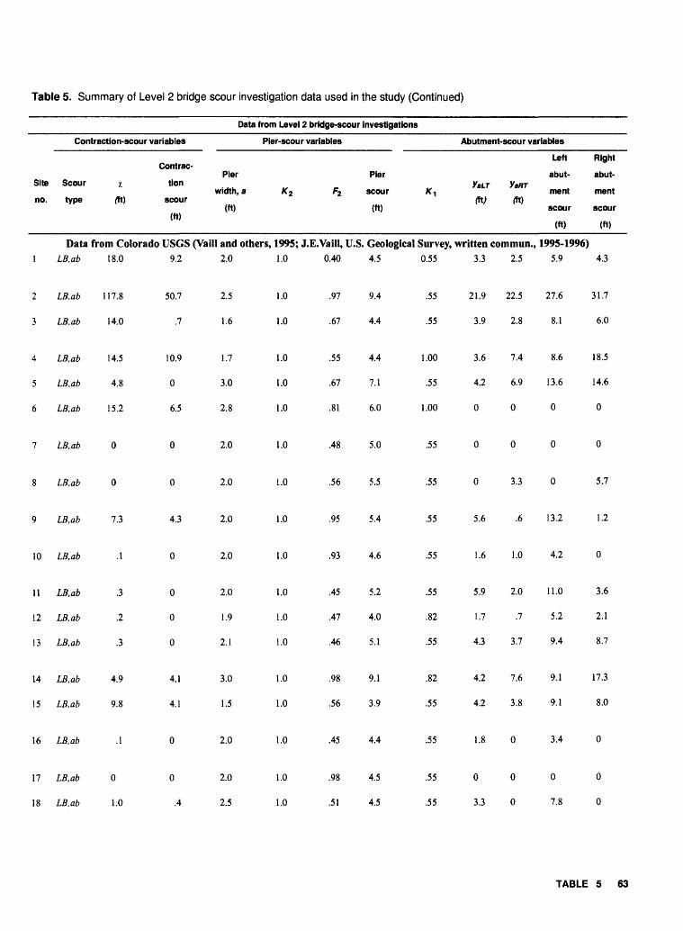
Table 5. Summary of Level 2 bridge scour investigation data used in the study (Continued)
Data from Level 2 bridge-scour investigations
Contraction-scour variables Pier-scour variables Abutment-scour variables
Left Right Contrac-
Pier Pier abut- abut- Site Scour x tion yaLT yafn
width, a K2 F2 scour K^ ment ment no. type (ft) scour (ft) (ft)
(ft) (ft) scour scour (ft)
_______________________________________________________________________(ft) (ft)Data from Colorado USGS (Vaill and others, 1995; J.E.Vaill, U.S. Geological Survey, written commun., 1995-1996)
1 LB.ab 18.0 9.2 2.0 1.0 0.40 4.5 0.55 3.3 2.5 5.9 4.3
2 LB,ab 117.8 50.7 2.5 1.0 .97 9.4 .55 21.9 22.5 27.6 31.7
3 LB.ab 14.0 .7 1.6 1.0 .67 4.4 .55 3.9 2.8 8.1 6.0
4 LB,ab 14.5 10.9 1.7 1.0 .55 4.4 1.00 3.6 7.4 8.6 18.5
5 LB.ab 4.8 0 3.0 1.0 .67 7.1 .55 4.2 6.9 13.6 14.6
6 LB.ab 15.2 6.5 2.8 1.0 .81 6.0 1.00 00 0 0
7 LB.ab 0 0 2.0 1.0 .48 5.0 .55 0 0 0 0
8 LB,ab 0 0 2.0 1.0 .56 5.5 .55 0 3.3 0 5.7
9 LB.ab 7.3 4.3 2.0 1.0 .95 5.4 .55 5.6 .6 13.2 1.2
10 LB.ab .1 0 2.0 1.0 .93 4.6 .55 1.6 1.0 4.2 0
11 LB.ab .3
12 LB,ab .2
13 LB.ab .3
14 LB.ab 4.9
15 LB.ab 9.8
16 LB.ab .1
17 LB.ab 0
18 LB,ab 1.0
0
0
0
4.1
4.1
0
0
.4
2.0
1.9
2.1
3.0
1.5
2.0
2.0
2.5
1.0
1.0
1.0
1.0
1.0
1.0
1.0
1.0
.45
.47
.46
.98
.56
.45
.98
.51
5.2
4.0
5.1
9.1
3.9
4.4
4.5
4.5
.55
.82
.55
.82
.55
.55
.55
.55
5.9
1.7
4.3
4.2
4.2
1.8
0
3.3
2.0
.7
3.7
7.6
3.8
0
0
0
11.0
5.2
9.4
9.1
9.1
3.4
0
7.8
3.6
2.1
8.7
17.3
8.0
0
0
0
TABLE 5 63

Table 5. Summary of Level 2 bridge scour investigation data used in the study (Continued)
Bridge- Flow Main Bridge structure Bridge Drain-
Site Bridge site name and open- class channel O10o Qbrgidentifica- length age area
no. location ing through slope (ft3/s) (ft3/s)tion number (ft) (mi2)
type bridge (ft/mi)
(mm)
Predomi
nant streambed
material
Data from Colorado USGS (Vaill and others, 1995; J.E. Vaill, U.S. Geological Survey, written commun., 1995-1996)-continued118 341
80 2 1
71 4 1
1.3 3.070 3,070
216 42.2 5,160 5,160
Sand/gravel
101
120
88
89
2 1
3 1
3 1
3 1
90 18.5 906 906
34 47.5 310 310
62 3.2 15,300 '4,750
920 24.8 4,450 4,450
10 31.7 8,320 '3,750
Gravel/cobble
Sand
Sand
Sand
Gravel/cobble
Fine sand
19 Rio San Antonio at P-13-D Route 142 near Manassa, Colo.
20 South Fork Rio N-10-V Grande River at Route 160 at South Fork, Colo.
21 South Fork South H-13-G Plane River at Route 285 near Fairplay, Colo.
22 Spring Creek at Route D-02-A 64 near Rangely, Colo.
23 Spring Creek at Route G-26-T 70 near Vona, Colo.
24 Uncompahgre River J-05-X at Route 348 near Olathe, Colo.
25 Unnamed Draw at G-20-C Route 86 near Limon, Colo. Data from Indiana USGS (Mueller and others, 1994; D.S. Mueller, U.S. Geological Survey, written commun., 1995-1996)
26 Big Blue River at 1-74-114-4192B 462.8 3 1 314 4.8 17,300 17,300 .49 Medium sand Interstate 74 near Shelbyville, Ind.
27 Buck Creek at State 32-18-5441A Road 32 at Yorktown, Ind.
28 East Fork White River 45-19-995D at U.S. Route 231 near Haysville, Ind.
29 East Fork White River 258-36-4912 at U.S. Route 258 near Seymour, Ind.
30 Kankakee River at 231-37-4980 U.S. Route 231 near Hebron, Ind.
31 Tippecanoe River at 24-91-3731A U.S. Route 24 at Mon- ticello, Ind.
32 Tippecanoe River at 331-50-6627 State Road 331 at Old Tip Town, Ind.
33 White River at State 358-42-6779 Road 358 near Edwardsport, Ind.
34 White River at U.S. 41-26-3917C Route 41 near Hazelton, Ind.
134
800
775
318.5
'-- 3 - 100
3 1 5,558
2,3474 4
3 3 1,445
469.5 2 1 1,768
223.5 3 1 390
499.5 4- 4.. 5;013
2,400 3 1 11,305
5.8 7,000 7,000 4.0 Fine gravel
.84 116,000 116,000 .20 Fine sand
1.9 98,000 39,100 1.0 Very coarse sand
1.1 6,800 6,800 1.0 Very coarse sand
2.6 25,000 25,000 4.0 Fine gravel
1.1 3,850 3,850 1.0 Very coarse sand
3.2 110,000 63,600 .40 Medium sand
.53 186,000 186,000 .50 Coarse sand
64 Method for Rapid Estimation of Scour at Highway Bridges based on Limited Site Data

Data from Level 2 bridge-scour investigations
Contraction-scour variables Pier-scour variables Abutment-scour variables
22 LB.ab
23 LB.ab
24 LB.ab
.1
4.2
.1
0
.2
0
1.0
2.1
1.3
1.0
1.0
1.0
.61
.28
.48
1.8
3.8
3.4
Right Contrac- Left abut-
Pler abut-Site Scour x tion Pier scour yaLT yafrr ment
width, a K 2 F2 K! mentno. type (ft) scour (ft) ft) ft) scour
(ft) scour
________«_________________________"" mData from Colorado USGS (Vaill and others, 1995; J.E. Vaill, U.S. Geological Survey, written commun., 1995-1996)-continued
19 LB.ab 6.1 5.0 1.0 1.0 .27 2.4 .82 3.1 3.0 4.3 4.5
20 LB.ab 0 0 1.8 1.0 1.01 4.3 1.00 1.5 .3 3.2 0
21 LB.ab 0 0 1.0 1.0 .55 3.5 .82 0 0 0 0
1.00 .2 .3 .8 .7
.55 1.8 2.7 2.5 9.7
.55 0 0 0 0
25 LB.ab 1.9 .3 2.0 1.0 .44 4.3 .55 2.0 2.0 4.6 4.0
Data from Indiana USGS (Mueller and others, 1994; D.S. Mueller, U.S. Geological Survey, written commun., 1995-1996)26 LB.c 0 0 3.5 1.0 .27 6.8 .55 4.3 3.6 7.5 6.9
CW.c 4.9 5.6CW.c 3.4 4.5
27 LB.c 3.4 0 3.7 1.0 .30 7.7 .82 0 0 0 0CW,c 2.2 1.1CW.c .7 1.1
28 LB.c 25.9 15.8 7.4 2.0 .22 28.8 .55 (12.4) 7.7 (31.6) 14.2CW.c (7.7) (11.1)CW.c (20.9) (25.7)
29 LB.c 12.6 13.7 2.5 1.0 .81 6.1 .55 (3.0) (3.9) (13.7) (11.5)CW,c 1.1 0CW.c .6 1.4
30 LB.ab (0) (.6) 2.0 1.0 .21 3.8 0000
31 LB.ab 2.4 2.9 6.0 1.0 .33 10.6 - 0000
32 LB.ab 2.7 2.1 2.0 1.0 .19 3.4 .55 1.6 5.8 4.9 14.1
33 LB.c 0 0 3.5 1.0 .32 8.8 .55 7.3 (6.2) 18.5 (24.4)CW.c 25.7 21.3CW.c 0 0
34 LB.c 13.6 10.5 4.7 1.0 .19 9.4 .55 3.7 (12.5) 11.6 (48.9)CW.c 6.2 8.2CW.c 6.4 7.8
TABLE 5 65

Table 5. Summary of Level 2 bridge scour investigation data used in the study (Continued)
Bridge- Flow Main Bridge structure Bridge Drain-
Site Bridge site name and open- class channel O100 Qbrgidentifica- length age area
no. location ing through slope (ft3/s) (fr/s)tion number (ft) (mi2)
type bridge (ft/mi)
(mm)
Predomi
nant streambed
material
Data from Indiana USGS (Mueller and others, 1994; D.S. Mueller, U.S. Geological Survey, written commun., 1995-1996)-continued35 5Whitewater River at 1-74-170-4684A and 968 3 1 1,344 5.3 62,200 62,200 .50 Coarse sand
Interstate 74 near Har- 4684JA rison, Ohio
Data from Iowa USGS (Fischer, 1995; E.E. Fischer, U.S. Geological Survey, written commun., 1995-1996)241 669 4.8 26,200 26,20036 Maple River at State 036911
Highway 175 near Mapleton, Iowa
37 Middle Raccoon 026131 River at State Highway 25 near Bayard, Iowa
38 Nodaway River at Clarinda, Iowa
39 Plane River near Diag onal, Iowa
40 West Nishnabotna 025531 River at State Highway 184 near Randolph, Iowa
Data from Mississippi USGS (W.T. Baldwin, U.S. Geological Survey, written commun., 1995-1996)
39 Medium sand
240
312
178
383
1 3
1 3
4 3
4 3
375
762
217
609
4.2 18,800 18,800
2.1 42,700 42,700
3.1 10,000 ^,800
2.2 49,500 '32,600
.34 Medium sand
.34 Medium sand
.47 Medium sand
.41 Medium sand
26.4 A and B 160 5.52 15.0 2,880 2,88041 Allbritton Creek at U.S. Interstate Highway 55 near Nor- field. Miss.
42 Bahala Creek at State 55.5 Highway 27 near Oma, Miss.
43 Buffalo River at State 7.2 Highway 563 at Wilkinson. Miss.
44 Hays Creek at State 39.3 Highway 407 at Winona, Miss.
45 Tonacana Creek at 121.4 U.S. Highway 80 at Chunky, Miss.
Data from Missouri USGS (R.J. Huizinga, U.S. Geological Survey, written commun., 1995-1996)
34 Medium sand
560
700
186
98
3 1
3
3 1
150
142
25.1
8.65 15.0
3.5 23,800 23.800
4.6 54.200 51.700
7.3 13,000 13,000
3,640 3,640
88 Coarse sand
30 Medium sand
30 Medium sand
.34 Medium sand
46 Honey Creek at State A-2497 Route 81 in Clark County, Mo.
47 Plane River at U.S. J-376 Route 136 in Nodaway County, Mo.
48 South Wyaconda J-780River at U.S. Route136 in ScotlandCounty, Mo.- mainbridge
48 Do--relief bridge J-780
145
445
220
135
1 21.4 4.5 5,600 5,600 .13 Fine sand
1 486 3.8 33,200 33,200 16 Coarse gravel
1 106 3.8 13,800 6 12,803 .57 Coarse sand
106 3.8 13,800 6997 .57 Coarse sand
66 Method for Rapid Estimation of Scour at Highway Bridges based on Limited Site Data

Data from Level 2 bridge-scour investigations
Contraction-scour variables
Site Scour
no. type
Contrac-
x tlon
(ft) scour
(ft)
Pier-scour variables
Pier
width, a
(ft)
K2 F2Pier scour
(ft)*1
Abutment-scour variables
YaLT
m;YaRT
(ft)
Right Left abut-
abut- ment
ment scour
scour (ft)
(ft)
Data from Indiana USGS (Mueller and others, 1994; D.S. Mueller, U.S. Geological Survey, written commun., 1995-1996)-continued35 LB.c
CW.cCW,c
4.7 4.9(0) (1-7)
5.8 7.0
4.0
Data from Iowa USGS (Fischer, 199536
37
38
39
40
LB,ab
LB.ab
LB.ab
LB.ab
LB.ab
8.3 5.4
5.9 2.1
6.0 4.1
13.9 6.5
7.7 0
3.0
3.0
4.0
1.3
3.0
1.0 .37 8.8 .55 (4.6) 0 (29.3) 0
; E.E. Fischer, U.S. Geological Survey, written commun., 1995-1996)1.0
1.3
2.0
1.0
1.0
.42
.35
.38
.23
.33
8.8
10.5
22.6
4.2
8.5
.55
.55
.55
.55
.55
(5.6)
(5.7)
(3.1)
(I- 3)
(0)
Data from Mississippi USGS (W.T. Baldwin, U.S. Geological Survey, written commun.41
42
43
44
45
LB.cCW.cCW.c
LB.cCW.cCW,cLB,cCW,cCW.cLB.cCW.cCW.cLB.cCW.cCW.c
6.3 3.31.0 1.21.2 1.3
14.0 7.80 00 00 00 03.6 3.14.0 1.40 00 04.0 3.21.0 1.32.5 2.3
1.2
4.0
5.0
2.5
2.0
1.0
1.0
1.0
1.0
1.2
.32
.33
.42
.31
.39
2.9
8.5
12.5
8.0
7.2
.55
.55
.55
.55
.55
3.5
7.9
4.3
2.9
3.2
Data from Missouri USGS (R.J. Huizinga, U.S. Geological Survey, written commun.,46
47
48
LB.ab
LB.cCW.cCW.cLB.ab
45.6 27.1
16.7 10.8.3 0
3.4 5.114.6 12.9
1.0
5.5
6.0
2.0
1.4
1.1
.64
.33
.23
9.1
20.2
12.3
.55
.55
.55
4.8
28.4
4.8
(2.0)
(6.8)
(4-1)
(2.7)
(0)
(14.0)
(11.9)
(12.5)
(8.6)
(0)
(15.8)
(14.1)
(15.5)
(15.0)
(0)
, 1995-1996)3.6
0.0
4.8
2.7
2.4
8.2
11.1
3.0
5.5
8.0
8.5
0
0
5.2
6.2
1995-1996)3.0
4.7
4.1
11.1
34.0
11.8
10.4
8.2
9.2
48 CW.d 2.7 1.5 2.0 .51 5.9 .82 2.6 2.5
TABLE 5 67

Table 5. Summary of Level 2 bridge scour investigation data used in the study (Continued)
Bridge- Flow Main Bridge structure Bridge Drain-
Site Bridge site name and open- class channel O100 Ob»identifies- length age area
no. location ing through slope (fr/s) (fr/s)tion number (ft) (mi2)
type bridge (ft/mi)
(mm)
Predomi
nant streambed
material
Data from Missouri USGS (R.J49 West Fork Grand J-795
River at State Route 46 in Worth County, Mo.
50 Badger Creek at U.S. 89,15 mile southeast of Browning, Mont.
51 Beaver Creek at U.S. 2, 6 miles west of Saco, Mont.
52 Beaver Creek over flow at U.S. 2,7 miles west of Saco, Mont.
53 Beaver Creek over flow at U.S. 2, 9 miles west of Saco, Mont.
54 Big Timber Creek at U.S. 191,2 miles north of Big Timber, Mont.
55 Bitterroot River atU.S. 12nearMissoula, Mont.
56 Boulder River at S 69 at Boulder, Mont.
57 Boulder Creek at State Route 1, near Maxville, Mont.
58 Cherry Creek at U.S. 2, 1 mile north of Glasgow, Mont.
59 Clark Fork at U.S. 12 at Missoula, Mont.
60 Clarks Fork Yellow- stone River at U.S. 310, 2 miles south of Bridger, Mont.
61 Cutbank Creek at U.S. 2 at Cut Bank, Mont.
62 Dearborn River at State Route 200,25 miles southwest of Simms, Mont.
63 East Rosebud River at State Route 78, 6 miles south of Absarokee, Mont.
P00003096+05771
Huizinga, U.S. Geological Survey, written commun., 1995-1996) continued288 3 1 229 4.4 25,100 25,100 .13 Fine sand
Data from Montana USGS303 3 4 239 20.5 13,000 5,666 8 Medium gravel
P00001492+07001 148 3 1 1.327 .26 13,500 76,750
P00007090+01161 and 62
P00069037+02861
POOO19049+00211
P00007095+00581
P00004023+07461
POOOO1254+01521
P00024102+05011
344 3 1 2,842 13.7 31,800 31,800
105
77
571
288
P00078026+02021 151
3 1
3 2
P00001540+03401 113 3 4
3 1
3 1
346 13.7 4,440 4,400 73
71.3 125.3 1,350 1,350 60
146 6.9 6,570 4,100
6,084 5.8 43,100 43,100
1,809 37.0 13,800 13,800 39
Fine sand/silt
P00001491+08241 89 3 2 1,327 .05 13,500 74,570 8 180 Grassland floodplain
P00001490+05771 88 3 1 1,327 .53 13,500 72,180 8 180 Grassland floodplain
P00045001+07641 126 3 4 119 37.0 5,750 5,340 5 Fine gravel
Coarse sand to medium gravel
Small cobbles
Very coarse gravel
Silty, clayey gravel
Gravel
Very coarse gravel
263 3 1 1,065 16.9 15,900 15,900 9 Medium gravel
177 3 1 235 26.4 12,100 12,100 2 Very fine gravel
145 51.2 4,210 4,210 58 Very coarsegravel
68 Method for Rapid Estimation of Scour at Highway Bridges based on Limited Site Data

Data from Level 2 bridge-scour investigations
Contraction-scour variables
Site Scour
no. type
49 LB.ab
50 LB.ab
51 LB.ab
52 CW,ab
53 CW.ab
54 LB.ab
55 LB.ab
56 LB.ab
57 CfKci
58 LB.ab
59 LB.aft
60 CW.ab
61 Z-B,aZ>
62 /,fl,a/>
Contrac-
X tion
(ft) scour
Data from Missouri13.7 6.8
6.7 0
7.8 2.8
0
0
10.1 6.5
0 0
8.2 3.9
0
0 ) 0
.2 0
0
5.9 4.2
10.0 5.7
Pier-scour variables
Pier
width, a K 2 F2
(ft)
Pier scour
(ft) 1
Abutment-scour variables
Left abut-
YaLT YaRT ment
(ft) (ft) scour
USGS (R.J. Huizinga, U.S. Geological Survey, written commun., 1995-1996)-continued5.0 1.9 .41 26.3 .55 (18.4) 8.1 (36.4)
Data from Montana USGS3.5 1.0 .42 6.7 .55
3.0 1.0 .49
2.0 1.0 .49
2.0 1.0 .60
2.0 1.0 .72
4.0 1.0 .41
2.0 1.8 .89
--
2.0 1.0 .56
3.7 1.7 .35
4.4 1.5 .90
5.5 1.7 .65
3.0 3.3 .77
6.9 .55
5.6 .55
4.7 .55
6.3 .55
9.0 .55
11.1 .55
.55
5.4 .55
16.8 .55
14.8 .55
24.4 .55
31.5 .55
2.9 3.5 7.2
2.6 3.2 6.6
5.3 5.1 0
3.8 4.0 0
4.1 4.2 5.9
000
1.3 1.1 2.9
0 .40
0 2.7 0
000
0 1.1 0
4.8 6.0 11.1
10.2 0 21.5
Right abut
ment
scour
13.5
8.7
7.0
0
0
10.2
0
3.6
1.9
7.3
0
3.2
14.6
0
63 LB.ab .2 0 3.0 1.2 .78 9.9 .55 0
TABLE 5 69

Table 5. Summary of Level 2 bridge scour investigation data used in the study (Continued)
Bridge- Flow Main Bridge structure Bridge Drain-
Site Bridge site name and open- class channel O10oidentif ica- length age area
no. location ing through ^ slope (ft3/s) (fr/s)tion number (ft) (ml2)
type bridge (ft/mi)
(mm)
Predomi
nant streambed
material
64 Gallatin River at U.S. 191,5 miles south of Gallatin Gateway, Mont.
65 Indian Creek at U.S. 287,7 miles south of Cameron, Mont.
66 Jefferson River at U. S. 10,2 miles west of Three Forks, Mont.
67 Lang Creek at U.S. 2, 19 miles southwest of Marion, Mont.
68 Little Blackfoot River at U.S. 12 and Burl ington Northern Rail road, 5 miles east of Garrison, Mont.
69 Little Blackfoot River at U.S. 12 near Garrison, Mont.
70 Pole Creek at U.S. 12, 3 miles southwest of Roundup, Mont.
71 Prickly Pear Creek at U.S. 12, near East Hel ena, Mont.
72 Sage Creek at U.S. 2, near Gildford, Mont.
73 Sandstone Creek at U.S. 12, near Plevna, Mont.
74 Spring Creek at State Route 35 1 mile east of Kalispell, Mont.
75 Sweetgrass Creek at U.S. 191,2 miles south of Melville, Mont.
76 Tenmile Creek at U.S. 12,5 miles west of Helena, Mont.
77 Tule Creek at U.S. 2, 10 miles east of Wolf Point, Mont.
78 West Fork Willow Creek at U.S. 2, 2 miles east of Devon, Mont.
Data from Montana USGS continuedP00050070+04611 252 3 1 825 33.5 10,700 10,700 95 Small cobbles
P00013030408711 81 3 1 65.3 47.7 1,820 1,820 135 Large cobbles
POOO13093406931 246 3 4 9,532 14.8 23,600 23,350 19 Coarse gravel
P00001080+04821 35 3 1 7.09 45.4 149 149 Fine sand to coarse gravel
P00008006402301 303 3 1 398 27.4 6,170 6,170 26 Coarse gravel
P00088001 +00271 138 3 4 407 34.3 6,580 4,900 4 Fine gravel
P00014165407861 71 3 1 389 22.7 4,800 '3,700 2 Very fine gravel
P00008049403341 74 3 1 251 34.3 2,160 2,160 5 Fine gravel
P00001353408951 116 3 4 701 2.7
P00002070407611 129 3 1 149 10.4
9,820 8,730 .09 Very fine sand
4,350 4,350 .15 Fine sand
P00052050404871 94 3 1 36.9 13.8 414 414 17 Coarse gravel
P00045018402631 184 3 1 89.0 22.2 3,420 3,420 4.5 Fine gravel
P00008036409441 100 83.3 58.1 2,130 1,820 50 Very coarsegravel
POOOO1601403641 116 3 1 144 5.8 6,650 6,650 .10 Very fine sand
POOOO1300401071 55 3 4 226 6.3 4,740 '2,050 .15 Fine sand
70 Method for Rapid Estimation of Scour at Highway Bridges based on Limited Site Data

Data from Level 2 bridge-scour investigations
Contraction-scour variables Pier-scour variables
Contrac- Pier
Site Scour x tion Pier scour width, a K 2 F2 K,
no. type (Tt) scour (ft) (ft)
(ft)
Data from Montana USGS continued64 CW.ab - 0 4.0 1.3 .77 12.2 .55
65 CW.ab - 0 1.5 1.0 .49 4.5 .55
66 LB.ab 1.0 .7 3.5 1.0 .70 9.0 .55
67 LB.ab .7 .4 1.0 1.0 .65 2.3 .55
68 LB.ab 1.8 0 3.0 1.7 .41 11.5 .55
Abutment-scour variables
Right Left abut-
abut- YaLT YaOT «nt
ment (Tt; (ft) scour
scour (ft)
(ft)
2.4 0 5.8 0
2.0 3.2 4.6 0
0 3.5 0 11.9
0000
2.8 0 0 0
69 LB,ab 1.6
70 LB.ab 10.9
71 LB.ab 2.7
74 CW.ab
75 LB.ab 3.7
1.4
6.0
1.4
0
3.0
3.0
2.8
72 LB.ab 54.4 36.2 3.0
73 LB.ab 2.9 2.8 3.0
3.0
3.0
1.0
1.0
3.8
1.2
1.0
2.5
.44 6.1
.35 7.5
.55 1.5 2.4 0
.43 29.9
.40 8.4
.22 4.3
.41 16.7
.55
.55
.55
.55
3.1 2.8 6.5
0 0 0
5.3
6.1
0
.55 7.2 7.1 13.4 10.0
.55 2.0 4.3 3.2 12.5
.5 1.2 1.0 3.1
2.5 2.2 4.9 5.1
76 CW.ab
77 LB.ab 15.1
78 LB.ab 4.3
11.1 2.8
3.2 1.0
1.0 .50 7.0
.55 1.3 .6 3.0 1.8
.55 2.4 2.7 5.7 6.3
1.0 .46 3.4 .55 3.2 2.1 6.3 5.4
TABLE 5 71

Table 5. Summary of Level 2 bridge scour investigation data used in the study (Continued)
Bridge- Flow Main Bridge structure Bridge Drain-
Site Bridge site name and open- class channel O100 Ohrgidentif ica- length age area
no. location ing through slope (ft3/s) (fr/s)tion number (ft) (mi2)
type bridge (ft/mi)
(mm)
Predomi
nant streambed
material
Data from Montana USGS continued79 Whitefish River at P00005128+00531 171 3 1 126 1.1 1,290 1,290 -- Clay to very
U.S. 93 at Whitefish, fine sand Mont.
80 Yellowstone River at POOO11020+04171 450 3 1 2,810 11.6 31,900 31,900 73 Small cobbles U.S. 89,11 miles southwest of Emi grant, Mont.
81 Yellowstone River at P00026001+02341 1,244 3 1 69,103 .50 154,600 154,600 - Silt State Route 23, 2 miles south of Sydney, Mont. Data from Montana MDT (D.R. Mclntyre and M.A. Goodman, Montana Department of Transportation, written commun., 1995-1996)
114 1 1
97
210
74
86
60
600
3 1 2,737
3 1 2,476
3 1 19,958
3 1 2,731
3 1
82 Assiniboine Creek at S00242006+0.0 MT 242,6 miles north of Malta, Mont.
83 Beaverhead River near BR9001(15) Barretts, Mont.
84 Big Hole River at BR9047(13) county road west of Melrose, Mont.
85 Clark Fork at State P00006082+0.759 986 Route 200 near Para dise, Mont.
86 ClarksFork L05304005+0.0 236 Yellowstone River 1 mile east of Silesia, Mont.
87 Judith River 6 miles LI4303007+0.7 northwest of Moore, Mont.
88 Little Bighorn River L02202012+0.2 11 miles southwest of Wyola, Mont.
89 Little Bighorn River 3 L02269000+0.1 miles southwest of Wyola, Mont.
90 Madison River - Mon- 100090278+0.857 336 2 1 2,551 tana Rail Link at Inter state 90, 1 mile east of Three Forks, Mont.
91 Milk River 1 mile BR9003(16) north of Lohman, Mont.
92 Mill Coulee near Sun F24-4( 11) 138 River, Mont.
93 Missouri River 8 miles P00025045+0.0 southeast of Wolf Point, Mont.
119 21.1 4,200 4,200
16.9 3,100 3,100
16.9 16,524 64,000
1.2 142,310 142,310
10.6 14,130 14,130
1
102 3 4
221
270
533 16.9 2,250 2,250
35.9 3,200 3.200
26.4 3,620 2,780
4.8 10,700 10,700
184 3 4 6,166 2.1 17,000 10,600
3 1 23.1 23.8 2,330 2,330
3 1 82,290 2.6 53,400 53,400
Sand to gravel
Gravel
Sand to medium gravel
Gravel
Silty sand
Silt/sand
Sand/gravel
72 Method for Rapid Estimation of Scour at Highway Bridges based on Limited Site Data

Contraction-scour variables
Data from Level 2 bridge-scour Investigations
Pier-scour variables Abutment-scour variables
Contrac-
Site Scour x lion
no. type (ft) scour
(ft)
Pier
width, a
(ft)
KyPier scour
(ft)
yaLT
Lett abut-
yaaT ment
(ft) scour
(ft)
Right abut
ment
scour
(ft)
79 LB.ab 1.1 .7
Data from Montana USGS--continued2.0 1.0 .08 2.9 .55
80 CW.ab 3.0 1.0 .59 7.8 .55 0 .9 0 2.5
81 LB,ab 9.5 9.1 9.0 2.4 .34 47.8 .55 7.4 0 19.3 0
Data from Montana MDT (D.R. Mclntyre,and M.A. Goodman, Montana Department of Transportation, written commun., 1995-1996)82 LB.ab 5.5 5.0 2.0 1.0 .71 5.0 1.00 2.4 2.5 6.0 6.7
83 LB.ab 1.3
84 LB.ab .1
1.0
.1
1.3
3.0
1.0 .75 3.0 .55 0 0 0 0
2.3 .46 12.0 .55 0 .6 0 0
85 LB.ab 12.5 7.5 10.0 1.7 .29 29.0 .55 0 0 0 0
86 LB.ab .6 1.0 3.5 1.0 .40 8.0 .55 2.9 2.7 8.0 11.0
87 LB.ab 2.3 1.0 1.3 1.0 .95 4.0 .55 3.1 1.8 5.0 3.0
88 LB.ab 1.3 1.0 .55 0 5.3 0 13.0
89 LB.ab 7.1 2.8 .55 1.9 3.3 5.5 11.3
90 LB.ab 3.2 3.0 5.0 1.0 .42 11.0 .55 0000
91 LB.ab 16.5 1.6 3.0 1.0 .21 6.4 .55 2.9 4.2 7.0 9.8
92 LB.ab 23.2
93 LB.ab A
11.2
0 4.0 1.0 .43 9.0
.55 3.9 4.3 8.2 8.9
.55 0 4.2 0 3.0
TABLE 5 73
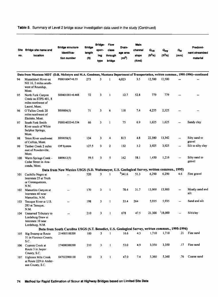
Table 5. Summary of Level 2 bridge scour investigation data used in the study (Continued)
Bridge- Flow MainBridge structure Bridge Drain-
Site Bridge site name and open- class channel Q,oo Q^rgidentified- length age area
no. location ing through . slope (fr/s) (fr/s)tion number (ft) (mi2)
type bridge (ft/mi)
(mm)
Predomi
nant streambed
material
Data from Montana MDT (D.R. Mclntyre and M.A. Goodman, Montana Department of Transportation, written commun., 1995-1996) continued94 Musselshell River on P00016047+0.55 273 3 1 4,023 3.5 12,500 12,500
NH 16, 2 miles south west of Roundup, Mont.
95 North Fork Canyon S00401001+0.468 72 3 1 CreekonSTPS401,8 miles northwest of Laurel, Mont.
96 O'Fallon Creek 20 BR9006(5) 71 3 6 118 miles northwest of Ekalaka, Mont.
97 South Fork Smith P00014033+0.554 66 3 1 75 River south of White Sulphur Springs, Mont.
98 Teton River southwest BR9050(5) 134 3 4 813 ofCollins, Mont.
99 Timber Creek 2 miles Off System 127.5 3 2 132 east of Powderville, Mont.
100 Warm Springs Creek - BR9012(5)
12.7 52.8 779 779
7.4 4,255 2,325
6.9 1,625 1,625
4.8 22,380 13,342
3.2 3,925 3,925
162 58.1 1,430 1,216
Sandy clay
Silty sand togravelSilt to silty clay
Silty sand to gravel
59.5 3 5 Cedar Street in Ana conda, Mont.
Data from New Mexico USGS (S.D. Waltemeyer, U.S. Geological Survey, written commun., 1995)101 Cuchillo Negro at - 520 3 1 9341.6 51.3 6,290 6,290 4.6 Fine gravel
Interstate 25 at Truth or Consequences, N.M.
102 Manuelito Canyon at -- 170 3 1 78.4 31.7 13,900 13,900 - Mostly sand and Interstate 40 near silt Manuelito, N.M.
103 Tesuque River at U.S. - 198 3 1 33.4 264 5,935 5,935 - Sand and silt 285 at Tesuque, N.M.
104 Unnamed Tributary to -- 210 3 1 678 47.5 21,300 '18,000 - Silt/clay Lordsburg Draw at Interstate 10 near Lordsburg, N.M.
Data from South Carolina USGS (S.T. Benedict, U.S. Geological Survey, written commun., 1995-1996)105 Big Swamp at Route 214005100200 100 3 1 16.6 4.3 1,710 1,710 .21 Fine sand
51 in Florence County, S.C.
106 Cypress Creek at 274000300200 210 3 1 53.0 4.9 3,350 3,350 .17 Fine sand Route 3 in Jasper County, S.C.
107 Eighteen Mile Creek 047022900100 150 3 1 47.0 7.4 5,360 5,360 .76 Coarse sand at Route 229 in Ander- son County, S.C.
74 Method for Rapid Estimation of Scour at Highway Bridges based on Limited Site Data

Contraction-scour variables
Data from Level 2 bridge-scour investigations
Pier-scour variables Abutment-scour variables
Site Scour
Contrac
tion
no. type (ft) scour
(ft)
Pier
width, a
(ft)
Pier scour
(ft)
Left abut-
Y»RT ment
(ft) (ft) scour
(ft)
Right
abut
ment
scour
(ft)
Data from Montana MDT (D.R. Mclntyre and M.A. Goodman, Montana Department of Transportation, written commun., 1995-1996)-continued94 LB.ab 6.9 5.0 1.3 1.0 .35 4.0 .55 4.2 5.6 9.0 11.0
95 LB.ab 1.5 2.0 .55 0 .7 0 1.0
96 LB,ab 14.4 12.0 .55 8.3 8.8 14.0 15.0
97 LB.ab 4.0 4.3 .55 2.9 1.8 8.8 4.4
98 LB,ab 22.4 12.6 4.0 1.0 .28 9.0
99 LB,ab (9.5) (15.0) 2.0 1.0 .41 4.0
.55 4.6 5.1 12.4 13.4
.55 6.4 5.8 13.0 10.0
100 LB.ab .6 0 1.7 1.0 .72 2.3 .55 0 0 0 0
Data from New Mexico USGS (S.D. Waltemeyer, U.S. Geological Survey, written commun., 1995)101 LB.ab 1.2 .9 1.2 1.0 .53 3.1 - (0) (0) (0) (0)
102 LB.ab 6.9 6.1 3.0 3.5 .47 28.3 (0) (0) (0) (0)
103 LB.ab .9 .6 3.0 2.8 1.16 25.3 (0) (0) (0) (0)
104 LB.ab 2.9 3.4 3.0 1.0 .95 8.0 1.00 13.5 18.0 11.8 15.
Data from South Carolina USGS (S.T. Benedict, U.S. Geological Survey, written commun., 1995-1996)105 CW.ab - 11.1 1.0 1.0 .31 2.5 .55 4.2 4.2 8.8 9.8
106 CW.ab 6.6 1.4 1.0 .16 3.1 .55 5.7 5.7 11.5 12.3
107 LB. c CW.c CW,c
3.5 3.5
.7 2.9 2.8
1.1 1.0 .42 3.5 .55 2.3 2.0 6.3 6.8
TABLE 5 75

Table 5. Summary of Level 2 bridge scour investigation data used in the study (Continued)
Bridge- Flow Main Bridge structure Bridge Drain-
Site Bridge site name and open- class channel Ow Qtirgidentif ica- length age area
no. location ing through _ slope (fr/s) (fr/s)tion number (ft) (mi2)
type bridge (ft/mi)
(mm)
Predomi
nant streambed
material
.22 Fine sand
.60 Coarse sand
Data from South Carolina USGS (S.T. Benedict, U.S. Geological Survey, written commun., 1995-1996)-continued108 Ox Swamp at Route 142052100300 175 3 1 32.7 4.0 2,530 2,530 .18 Fine sand
521 in Clarendon County, S.C.
109 South Tyger River at 421008530100 320 3 3 96.2 3.5 7,940 7,940 .60 Coarse sand Route 85 in Spartanburg, S.C.
110 Tools Fork Creek at 464032200500 150 3 1 13.4 9.0 3,820 3,820 .92 Coarse sand Route 322 in York County, S.C.
Data from Texas USGS (D.D. Dunn, U.S. Geological Survey, written commun., 1995-1996)111 Brazos River at State - 972 3 1 34,400 6.3 166,500 166,500 .35 Medium sand
Highway 159 near Hempstead, Tex.
112 Colorado River atState Highway 71 near Columbus, Tex.
113 Guadalupe River at State Highway 80 near Belmont, Tex.
114 Guadalupe River at U.S. 183 near Hochheim, Tex.
115 Trinity River at State Highway 7 near Crockett, Tex.
Data from Vermont USGS (J.D. Ayotte and S.A. Olson, U.S. Geological Survey, written commun., 1995-1996)116 Ayers Brook at Town BRAITH00230012 28 1 5
Highway 023, Braintree, Vt.
117 Black River at Town IRASTH00050006 70 1 1 Highway 005, Irasburg, Vt.
118 Black River at Town IRASTH00080020 88 1 1 Highway 008, Irasburg, Vt.
119 North Bridgewater WODSTHOO180022 40 1 1 Brook at Town Highway 018, Woodstock, Vt.
120 Ompompanoosuc NORWTH00030046 100 1 1 River at Town Highway 003 (VT 132), Norwich, Vt.
121 Second Branch White RANDTH00660034 57 1 6
873 3 1 1041,640 1.6 114,600 6 109,926 .50 Coarse sand
1,136 3 1 2,036 1.1 60,300 60,300
758 3 44 4,094 2.6 152,000 83,240
687 3 1 13,911 .5 116,500 674,117 .20 Fine sand
sol18.8 15.8 1,670 970 3.3 Very fine gravel
91.1 79 3,530 3,530 171 Large cobbles
110 11
434 180
3,800 3,800 35 Very coarse gravel
1,100 1,100 44 Very coarse gravel
135 15.8 2,600 2,600 .50 Coarse sand
51.3 10 7,660 3,490 .67 Coarse sandRiver at Town High way 066, Randolph, Vt.
76 Method for Rapid Estimation of Scour at Highway Bridges based on Limited Site Data

Contraction-scour variables
Data from Level 2 bridge-scour Investigations
Pier-scour variables Abutment-scour variables
Site Scour x
no. type (ft)
Contrac-
tion
scour
Pier
width, a
(ft)
K 2Pier scour
(ft)
Left abut-
yaLT yafrr ment
(K) (ft) scour
Right
abut-
ment
scour
Data from South Carolina USGS (S.T. Benedict, U.S. Geological Survey, written commun., 1995-1996)-continued108 CW.ab - 6.9 2.0 1.0 .20 4.0 .55 5.4 5.4 11.1 10.8
109 LB,c (.4) (2.8) 1.7 1.0 .18 3.8CW.c 1.1 2.1CW.c 0 0
110 CW,c 9.0 7.8 2.3 1.3 .28 6.2CW.c 3.9 4.4CW.c (4.6) (7.7)
.55 0 10.7 0 21.3
.55 5.1 6.7 8.7 15.4
Data from Texas USGS (D.D. Dunn, U.S. Geological Survey, written commun., 1995-1996)(0) (0) (0)
.55 10.8 0
.55
.55
(0)
.19 6.6 n .55,1.0 9.2 5.8 14.9 9.0
19.4 0
111 LB.c 0 0 6.0 2.5 .22 32.7 .55CW.c 1.8 2.6CW.c 0 0
112 LB.c 1.9 1.0 2.5 1.0CW.c 2.5 3.8CW.c 0 0
113 LB.c 5.6 5.4 2.5 1.1 .20 7.4CW.c 12.2 14.4CW.c 4.4 5.6
114 LB.c (3.6) (5.5) 3.0 1.0 .28 7.7CW.c 0 0CW,c (.1) (6.7)
115 LB.c 39.7 8.8 4.0 1.0 .12 8.0CW,c 0 0CW.c 0 0
Data from Vermont USGS (J.D. Ayotte and S.A. Olson, U.S. Geological Survey, written commun., 1995-1996)116 CW.ab - 5.4 -- -- -- -- H 1.0,.82 1.8 4.8 6.5 15.2
12.1 11.2 18.5 18.2
7.4 3.6 11.2 4.4
117 CW.ab .82 2.5 4.1 11.5 14.4
118 CW.ab U 1.0,.82 4.4 4.2 15.9 12.7
119 LB.ab 1.0 .82 2.2 2.6 5.3 5.6
120 LB.ab 2.9 2.2 4.5 1.7 .57 13.0 .82 3.8 3.1 9.7
121 LB.ab 22 A 8.0 n .82,1.0 2.7 3.9 11.2 17.2
TABLE 5 77
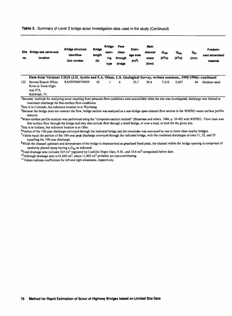
Table 5. Summary of Level 2 bridge scour investigation data used in the study (Continued)
Bridge- Flow MainBridge structure Bridge Drain- Predoml-
Site Bridge site name and open- class channel O100 Qbrg D^identifies- length age area , , nant streambed
no. location ing through slope (fp/s) (fl3/s) (mm)tion number (ft) (mi2) material
type bridge (ft/mi)
Data from Vermont USGS (J.D. Ayotte and S.A. Olson, U.S. Geological Survey, written commun., 1995-1996)-continued122 Second Branch White RANDTH00730039 42 1 6 53.7 50.4 7,910 2,407 .44 Medium sand
River at Town High way 073,
Randolph, Vt._______________________________________________________________________ 'Because methods for analyzing scour resulting from pressure-flow conditions were unavailable when the site was investigated, discharge was limited to
maximum discharge for free-surface flow conditions. 2Site is in Colorado, but reference location is in Wyoming. 3Because the bridge does not contract the flow, bridge section was analyzed as a non-bridge open-channel flow section in the WSPRO water-surface profile
analysis. 4Water-surface profile analysis was performed using the "composite-section method" (Shearman and others, 1986, p. 39-40) with WSPRO. Flow class was
free-surface flow through the bridge and may also include flow through a relief bridge, or over a road, or both for the given site. 5Site is in Indiana, but reference location is in Ohio.6Portion of the 100-year discharge conveyed through the indicated bridge and the remainder was conveyed by one or more other nearby bridges. 7Values equal the portion of the 100-year peak discharge conveyed through the indicated bridge, with the combined discharges of sites 51, 52, and 53
equalling the 100-year discharge. 8 While the channel upstream and downstream of the bridge is characterized as grassland flood plain, the channel within the bridge opening is comprised of
randomly placed riprap having a DSQ as indicated. 9Total drainage area includes 325 mi2 regulated by Cuchillo Negro Dam, N.M., and 16.6 mi2 unregulated below dam.I ° Although drainage area is 41,640 mi2, about 11,403 mi2 probably are non-contributing.II Values indicate coefficients for left and right abutments, respectively.
78 Method for Rapid Estimation of Scour at Highway Bridges based on Limited Site Data

Data from Level 2 bridge-scour investigations
Contraction-scour variables Pier-scour variables Abutment-scour variables
Right Contrac- Left abut-
Pier abut- Site Scour x *'on Pier scour yaLT ya^r men\
width, a K2 F2 K-t ment no. type (ft) scour (ft) (ft) (ft) scour
(ft) scour (ft) (ft)
__________________________________________________________________________(ft)Data from Vermont USGS (J.D. Ayotte, and S.A. Olson, U.S. Geological Survey, written commun., 1995-1996)-continued
122 LB.ab 28.0 3.3 -- -- - - .82 1.4 5.2 6.6 19.7
TABLE 5 79