Methanol exchange between grassland and the atmosphere - BGD

BGD4, 125–164, 2007

Methanol exchangebetween grasslandand the atmosphere

A. Brunner et al.

Title Page

Abstract Introduction

Conclusions References

Tables Figures

J I

J I

Back Close

Full Screen / Esc

Printer-friendly Version

Interactive Discussion

EGU

Biogeosciences Discuss., 4, 125–164, 2007www.biogeosciences-discuss.net/4/125/2007/© Author(s) 2007. This work is licensedunder a Creative Commons License.

BiogeosciencesDiscussions

Biogeosciences Discussions is the access reviewed discussion forum of Biogeosciences

Methanol exchange between grasslandand the atmosphereA. Brunner, C. Ammann, A. Neftel, and C. Spirig

Agroscope Reckenholz-Tanikon Research Station ART, Reckenholzstrasse 191, 8037 Zurich,Switzerland

Received: 8 January 2007 – Accepted: 17 January 2007 – Published: 26 January 2007

Correspondence to: A. Neftel ([email protected])

125

http://www.biogeosciences-discuss.net

http://www.biogeosciences-discuss.net/4/125/2007/bgd-4-125-2007-print.pdf

http://www.biogeosciences-discuss.net/4/125/2007/bgd-4-125-2007-discussion.html

http://www.copernicus.org/EGU/EGU.html

BGD4, 125–164, 2007


A. Brunner et al.

Title Page



Tables Figures

J I

J I

Back Close

Full Screen / Esc



EGU

Abstract

Concentrations and fluxes of methanol were measured above two differently managedgrassland fields (intensive and extensive) in central Switzerland during summer 2004.The measurements were performed with a proton-transfer-reaction mass-spectrometerand fluxes were determined by the eddy covariance method. The observed methanol5

emission showed a distinct diurnal cycle and was strongly correlated with global radia-tion and water vapour flux. Mean and maximum daily emissions were found to dependon grassland species composition and, for the intensive field, also on the growing state.The extensive field with a more complex species composition had higher emissionsthan the graminoid-dominated intensive field, both on an area and on a biomass basis.10

A simple parameterisation depending on the water vapour flux and the leaf area indexallowed a satisfying simulation of the temporal variation of methanol emissions over thegrowing phase. Accumulated carbon losses due to methanol emissions accounted for0.024 and 0.048% of net primary productivity for the intensive and extensive field, re-spectively. The integral methanol emissions over the growing periods were more than15

one order of magnitude higher than the emissions related to cut and drying events.

1 Introduction

Methanol is one of the most abundant oxygenated volatile organic compounds in theatmosphere with typical surface concentrations of 1–10 ppbv over land and marineconcentrations of 0.5–1.5 ppbv (Jacob et al., 2005; Singh et al., 2000). Its role in atmo-20

spheric chemistry is significant as it influences the concentrations of various oxidants.Formaldehyde, ozone and peroxy radical concentrations are enhanced while OH rad-ical levels are decreased through the atmospheric reactions of methanol. The effectsare most pronounced in the free troposphere, where concentrations of other reactiveorganic compounds are small while methanol still prevails due to its comparably long25

atmospheric lifetime of 8–12 days (Tie et al., 2003).

126





BGD4, 125–164, 2007


A. Brunner et al.

Title Page



Tables Figures

J I

J I

Back Close

Full Screen / Esc



EGU

11–20% of the methanol in the atmosphere are of anthropogenic and atmosphericorigin, while the major part (80–89%) is of biogenic origin (Heikes et al., 2002; Gal-bally and Kirstine, 2002; Jacob et al., 2005). Processes leading to biogenic methanolemission are manifold. Several authors reported methanol emission as part of theplant metabolism particularly during growth (e.g. Schulting et al., 1980; Isidorov et5

al., 1985; MacDonald et al., 1993; Fall and Benson, 1996; Karl et al., 2002). Plantstresses like hypoxia, frost and high ozone concentrations can also cause methanolemissions (Fukui and Dorskey, 1998; von Dahl et al., 2006). In addition senescing,injuring (e.g. herbivore attacks, cutting) and drying of plant leaves as well as biomassburning are known to be sources of methanol (de Gouw et al., 1999; Warneke et al.,10

2002; Karl et al., 2005; Loreto et al., 2006; Holzinger et al., 1999 and 2004). Themajor removal processes for methanol are oxidation by OH radicals (in the gas and theaqueous phase) as well as dry and wet deposition (Monod et al., 2000; Heikes et al.,2002; Galbally and Kirstine, 2002; Jacob et al., 2005).

Concerning the metabolism related methanol release, Frenkel et al. (1998) found that15

methanol within the leaf is mostly produced as a consequence of the demethylationof the pectin matrix, a necessary step in the extension of the cell walls during plantgrowth. On the basis of the pectin content, Galbally and Kirstine (2002) distinguishedbetween two major cell wall types with a high or low potential for methanol release. Inparticular graminoids of the family poaceae, to which the main forage crops belong,20

are low methanol emitters. Most other plants have cell walls with a higher potentialof methanol release. To a minor extent, methanol can be the result of an enzymaticcleavage of lignin (see Fall and Benson, 1996, and references therein), demethylationof DNA (see Galbally and Kirstine, 2002, and references therein) and protein repairpathways (Fall and Benson, 1996).25

Nemecek-Marshall et al. (1995) described a distinct dependence of methanol emis-sion on stomatal conductance. Niinemets and Reichstein (2003a, b) and Niinemets etal. (2004) relate this behaviour to a temporary storage of methanol in the liquid pools ofthe leaves due to its high solubility. As a consequence of this buffering effect, the pro-

127





BGD4, 125–164, 2007


A. Brunner et al.

Title Page



Tables Figures

J I

J I

Back Close

Full Screen / Esc



EGU

duction and release of methanol are not directly coupled. Because the understandingof the mechanisms controlling the methanol emission is still limited, reliable long-termemission datasets with a high temporal resolution are desirable for a variety of differentecosystems.

Until now, field measurements of biogenic methanol emissions have mainly been5

performed over different types of forest (e.g. Fehsenfeld et al., 1992; Schade andGoldstein, 2001; Spirig et al., 2005; Karl et al., 2005; Schade and Goldstein, 2006).Grasslands cover one quarter of the earth’s land surface (Graedel and Crutzen, 1993).Apart from studies concerning the methanol emissions due to harvesting (De Gouwet al., 1999; Karl et al., 2001; Warneke et al., 2002) only few long-term flux studies10

exist for grassland (Kirstine et al., 1998; Fukui and Doskey, 1998). These are based onchamber measurements characterised by a low time resolution.

In this work we present methanol concentration and flux measurements above twomanaged grassland fields during the summer 2004. The fields are located on theSwiss central plateau and differ in management intensity and species composition.15

Methanol was detected continuously with high temporal resolution by proton-transfer-reaction mass-spectrometry and the fluxes were determined by the eddy covariancetechnique on the ecosystem scale. We focus on the temporal variation of fluxes ob-served throughout a growing phase and attempt to parameterise it in a simple waybased on available environmental parameters.20

2 Materials and methods

2.1 Site and measurement description

The experimental site is located near Oensingen on the Swiss Central Plateau(47◦17′ N, 7◦44′ E; 450 m a.s.l.). The prevailing climate is temperate continental, withan average annual rainfall of 1100 mm and a mean annual air temperature of 9◦C.25

The experimental field was converted from arable rotation to permanent grassland in

128





BGD4, 125–164, 2007


A. Brunner et al.

Title Page



Tables Figures

J I

J I

Back Close

Full Screen / Esc



EGU

2001 and is part of the projects on carbon and greenhouse gas budgets CarboEu-rope and Greengrass (for details see Ammann et al., 2006; Flechard et al., 2005).It has a size of 104 m×146 m and had been split into two parts which differ in man-agement and species composition: (a) an intensively managed part (in the followingreferred to as intensive or INT) and (b) an extensively managed part (extensive or5

EXT). The intensive part is cut four times a year and is fertilised after each cut, al-ternately with slurry and ammonium nitrate. It is mainly composed of three species:two graminoids (Alopecurus pratensis, Lolium perenne), and one legume (Trifoliumrepens). The extensive part is cut three times a year and is not treated with any fer-tilizer. It is largely composed of twelve species: six graminoids (Alopecurus pratensis,10

Arrhenatherum elatius, Dactylis glomerata, Lolium perenne, Poa pratensis, and Poatrivialis), four forbs (Chrysanthemum leucanthemum, Stellaria media, Taraxacum offic-inale, and Tragopogon orientalis), and two legumes (Lotus corniculatus, and Trifoliumrepens).

Standard monitoring at the site included a weather station continuously measuring15

global radiation (Rg), air temperature (Tair), relative humidity (RH), barometric pres-sure, rainfall, wind speed and wind direction. Leaf area index (LAI) of both fields wasdetermined every 2–3 weeks by an optical method (LAI-2000, LI-COR, Lincoln NE,USA). Fluxes of CO2 (FCO2) and water vapour (FH2O) were routinely measured on bothfields during the whole summer by eddy covariance using a combination of a sonic20

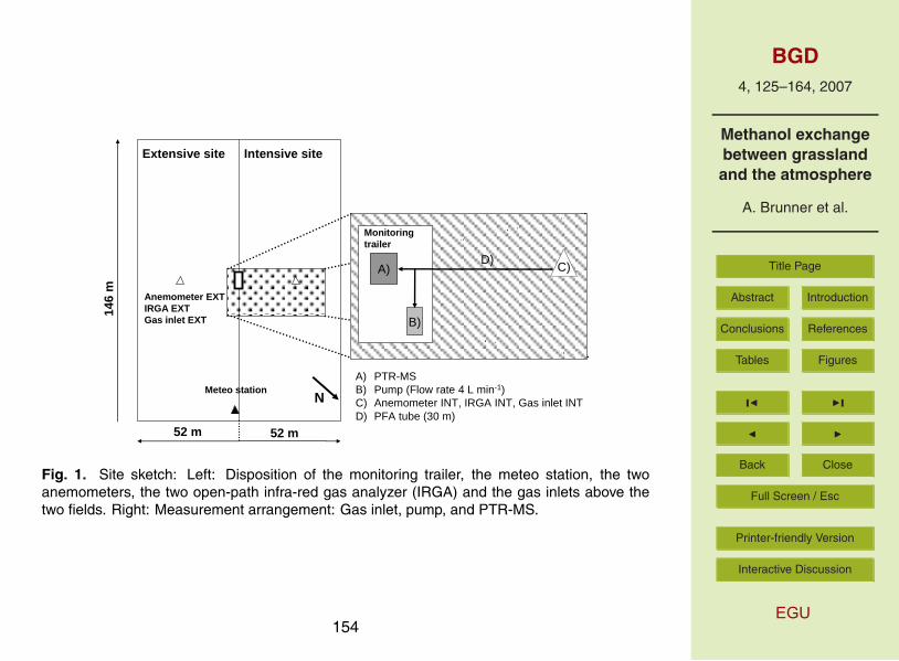
anemometer (Gill, Solent, Lymington, UK) and an open-path infra-red gas analyzer(IRGA, LI-7500, LI-COR, Lincoln NE, USA). Figure 1 shows a sketch of the fields andthe technical facilities. The CO2 assimilation rates of each field were calculated fromthe respective CO2 fluxes by a specific gap filling and partitioning algorithm (Ammannet al., 2006).25

Methanol concentration (cMeOH) and flux (FMeOH) measurements above the intensivefield were conducted from 25 June until 1 August 2004, between the second and thethird cut of the year. Above the extensive field, methanol measurements were per-formed from 7 until 24 June 2004 and from 2 August until 7 September 2004, covering

129





BGD4, 125–164, 2007


A. Brunner et al.

Title Page



Tables Figures

J I

J I

Back Close

Full Screen / Esc



EGU

periods between the first and the second cut of the year (Fig. 2). In the following,methanol fluxes of the first three days after a cut are referred to as cut-related emis-sions, the fluxes afterwards until the next cut as growth-related emissions. The corre-sponding periods are called cut and growing period, respectively (Fig. 2).

2.2 PTR-MS measurements5

Methanol was measured by a commercially available proton-transfer-reaction massspectrometer (PTR-MS, Ionicon Analytik GmbH, Innsbruck, A). The instrument andits operating mode had been described in detail by Lindinger et al. (1998). Here wedescribe the experimental setup from the gas inlet to the instrument and go then intospecifics of the PTR-MS used in this field study.10

Ambient air, collected 1.2 m above ground, was pulled through a 30 m PFA-tube(1/4” O.D., I.D. 3.5 mm) by a vacuum pump with a flow rate of 4 L min−1. The resi-dence time in the tube was about 4.3 s. The tube was connected to the PTR-MS inlet(Fig. 1), where the sampled air was introduced directly into a drift tube. There the reac-tion between H3O+ ions (generated by electrical discharge of pure water vapour) and15

methanol molecules produced methanol-H+ ions (mass 33) and water molecules. Themethanol-H+ ions were then detected by a quadrupole mass filter in conjunction with asecondary electron multiplier (SEM, MC-217, Mascom GmbH, Bremen, D).

The PTR-MS used in this field study corresponds to the PTR-MS-HS type, featur-ing three turbo pumps for increased sensitivity and a drift tube (equipped with Teflon20

rings) optimized for fast time response and minimal interactions with polar compounds(Spirig et al., 2005). It was running under the following conditions: pressure drift tubeof 2.1 mbar and drift tube voltage of 550 V, resulting in an electrical field strength togas density ratio (E/N) of 122 Td. Five to eight masses were analysed in rotation: m21(mass of the protonated ion with 21 atomic mass units (amu) which corresponds to a25

protonated water molecule with an O18-isotope), m33 (methanol), m37 (water cluster:H2O · H3O+), m45 (acetaldehyde), m59 (acetone and propanal), m73 (methyl ethylketone and butanal), m81 (fragments of hexenals and monoterpenes), and m83 (frag-

130





BGD4, 125–164, 2007


A. Brunner et al.

Title Page



Tables Figures

J I

J I

Back Close

Full Screen / Esc



EGU

ments of C6-alcohols). The integration time for a single compound was 50 (for m21and m37) to 200 ms (for all other compounds), resulting in a measurement of eachcompound every 0.7 to 1.3 s (Ammann et al., 2006).

The PTR-MS was calibrated with a gas standard (Apel-Riemer Environmental, Inc.,Denver CO, US), that included methanol. It was dynamically diluted with air generated5

by a zero air generator (ChromGas Zero Air Generator, model 1000, Parker HannifinCo., Haverhill MA, US). The absolute accuracy of the methanol concentration mea-surement is estimated to be ±20% due to mass flow controller and gas standard un-certainties.

2.3 Eddy covariance method10

The EC flux measurement with the PTR-MS was done with the same sonic anemome-ters as used for the routine CO2 and H2O flux measurements (see above) placed inthe middle of the grassland fields. The inlet for the PTR-MS sample air was placedclose to the sonic sensor head (distance 15 cm). To calculate the fluxes we used theEC calculation method described by Spirig et al. (2005). The PTR-MS measurement of15

the methanol ion (for 0.2 s) is regarded to be representative for the whole interval of themeasuring cycle (0.7–1.3 s). Technically, this is implemented by simply repeating thePTR-MS mass concentrations of a particular cycle until the next PTR-MS data pointis available. After this procedure, similar equidistant time series (time resolution ∆t =0.05 s) of sonic wind data and methanol concentration are available for the flux calcu-20

lations. Following the eddy covariance method the vertical flux of a trace gas Fc (or ofanother scalar quantity) is calculated as the covariance of the discrete time series ofthe vertical wind w(t) and the concentration c(t) over an averaging period Ta of typically30 min.:

Fc = covwc(τdel) =(∆tTa

)·

Ta∑t=0

[w(t) − w] ·[c(t − τdel) − c

](1)25

131





BGD4, 125–164, 2007


A. Brunner et al.

Title Page



Tables Figures

J I

J I

Back Close

Full Screen / Esc



EGU

The overbars denote the arithmetic mean of the averaging period. The two time seriesare adjusted to each other by a delay time τdel that accounts for the residence timein the air sampling tube and possible time difference between the data acquisitionsystems that are different for the PTR-MS and the sonic anemometer. The time delaywas calculated for each measuring interval separately by determining the maximum in5

the covariance function of the flux. In cases where no clear maximum could be foundwithin the physically possible limits of the lag, an interpolated best guess for the lagwas used (Ammann et al., 2006).

Beside the delay time, the inlet tube also led to a damping of high-frequent turbulentfluctuations of the trace gas concentrations before the detection by the PTR-MS. Ad-10

ditional high-frequency damping effects of the PTR-MS signals stem from the limitedtime resolution and the corresponding data treatment, as well as from the separationdistance between the sampling tube inlet and the anemometer sensor. These dampingeffects were quantified and corrected for by the empirical ogive method described indetail by Ammann et al. (2006). The high-frequency damping mainly depended on the15

wind speed and ranged between 25% (low wind speed) and 55% (high wind speed).The detection limit of the EC fluxes was determined empirically from the standard devi-ation of the covariance function at large delay times according to Wienhold et al. (1995).It was estimated on average to 0.3 nmol m−2 s−1 and 0.8 nmol m−2 s−1 for the measure-ments above the intensive and extensive field, respectively. The values are roughly20

proportional to the mean fluxes of the two fields.

132





BGD4, 125–164, 2007


A. Brunner et al.

Title Page



Tables Figures

J I

J I

Back Close

Full Screen / Esc



EGU

3 Results

3.1 Measurements above the intensively managed field

3.1.1 Weather conditions and vegetation development

During the summer 2004, average temperatures and precipitation at the measurementsite were near the long-time seasonal mean. Above the intensive field methanol con-5

centrations and fluxes were measured between 25 June and 1 August. As illustrated inFig. 3, weather conditions during this time were characterised by two periods of con-trasting weather. The first period (till 13 July) showed relatively low temperatures inconnection with rain and clouds; it was followed by a mostly clear sky and dry periodtill the end of July.10

The intensive field was cut on 25 June (2nd cut of the year). The hay was removedfrom the field on 26 June. The average dry matter yield of this growth was 0.32 kg m−2.After the fertilisation with slurry on 1 July, the grassland grew 8 weeks until the nextcut on 28 August. On the same day the grass was processed to silage. The averagedry matter yield of this growth was 0.19 kg m−2. The leaf area index increased from15

0.3 m2 m−2 on 25 June (just after the cut) to 3.7 m2 m−2 on 19 August (last measure-ment before the 3rd cut) (see Fig. 2).

3.1.2 Concentrations

During the measurements on the intensive field, the concentrations were between 1.7and 26.9 ppbv (Fig. 3), with an overall average concentration of 6.45 ppbv. Low con-20

centrations were mainly detected during or after rainfall (e.g. 05–13 July). High con-centrations were found shortly after the cut (28 June) and at the end of July. Figure 4ashows methanol concentrations plotted against the time of day. The mean concen-tration shows a characteristic diurnal variation. Highest concentrations were found inthe late evening hours. They slowly decreased during the night and increased again25

133





BGD4, 125–164, 2007


A. Brunner et al.

Title Page



Tables Figures

J I

J I

Back Close

Full Screen / Esc



EGU

around 07:00 LT. During daytime the concentrations dropped continuously to reach low-est levels around 18:00 LT. Figure 4 shows highest methanol concentrations coincidingwith lowest wind speeds.

3.1.3 Fluxes

Methanol fluxes measured on the intensive grassland field are shown in Fig. 3. Dur-5

ing the whole period methanol was emitted by the field, and no significant depositionfluxes could be observed. The highest fluxes (up to 30 nmol m−2 s−1) were measureddirectly after the cut on 25 June, which can be explained by amplified emissions due toplants wounding (De Gouw et al., 1999). Afterwards the fluxes were generally below10 nmol m−2 s−1. They showed a clear diurnal cycle with the maximum around midday10

and the minimum during night. The diurnal cycle followed the global radiation and thewater vapour flux in shape and strength. This is most obvious for the period 5–13 Julythat exhibit a very similar day-to-day variation of all quantities. The liquid manure treat-ment on 1 July let the emission of methanol rise temporarily with maximum emission of12.4 nmol m−2 s−1. Measured methanol fluxes during night were mostly close to zero15

and/or below the detection limit of the EC method.Up to three days after a cut, methanol fluxes seem to be mostly triggered by the injury

and the hay drying process. In order to investigate methanol emission during growthwe excluded the data of the first three days after the cut. For the growing period 28.06–01.08.04, scatter plots of the methanol flux with various potential controlling parameters20

are shown in Fig. 5. They suggest a linear correlation between the methanol flux andthe global radiation, the water vapour flux, and the sensible heat flux, respectively.These three correlations are positive. Further a logarithmic dependence can be seenbetween the methanol flux and the assimilation rate. Table 1 gives an overview ofall calculated correlations coefficients r2. Highest correlations exist between methanol25

flux and global radiation (r2=0.73), and water vapour flux (r2=0.71), respectively. Thecorrelation of methanol flux and air temperature is low. It is likely to be a consequenceof the diurnal cycle of the temperature which is similar but delayed in comparison to Rg

134





BGD4, 125–164, 2007


A. Brunner et al.

Title Page



Tables Figures

J I

J I

Back Close

Full Screen / Esc



EGU

and FH2O. The resulting hysteresis becomes evident when looking at individual daysas shown in Fig. 5f.

In order to study the longer-term development of methanol emission, the strongshort-term variability (diurnal and day-to-day) was sought to be reduced by dividingthe observed methanol fluxes by the respective water vapour fluxes:5

γ(t) =FMeOH(t)

FH2O(t)(2)

As shown in Fig. 3, the water vapour flux shows diurnal and weather induced day-to-day variations but no systematic long-term trends. When plotting the ratio γ(t) for theintensive grassland (Fig. 6a), a systematic decrease with time was found. γ almostlinearly declined from an initial value of about 1.1 nmol mmol−1 one week after the cut10

down to 0.4 nmol mmol−1 within the first four weeks of growth. Afterwards (Fig. 6a,Phase A), it stayed more or less constant. Thus normalised by the water vapour flux,methanol emission of the grassland ecosystem (per unit ground area) was three timeshigher shortly after the cut than four weeks later. If the methanol flux is related tothe growing leaf area, the decrease in γ/LAI is even more pronounced (Fig. 6b) with15

an almost exponential drop from an initial value of about 1.5 to only 0.2 nmol mmol−1

within the first four weeks, indicating that the young grassland vegetation emitted up to7.5 times more methanol per leaf area than the mature one.

3.2 Measurements above the extensively managed field

3.2.1 Weather conditions and vegetation development20

Above the extensive field, methanol concentrations were measured between 7 Juneand 7 September 2004 including the second growing period between the first andsecond cut. The measurements were not continuous due to an inserted measurementperiod above the intensive field (25 June–1 August). The weather conditions during themeasurements above the extensive field were characterised by a relatively cold period25

135





BGD4, 125–164, 2007


A. Brunner et al.

Title Page



Tables Figures

J I

J I

Back Close

Full Screen / Esc



EGU

in the middle of June and a relatively wet period starting in mid-August and lasting fortwo weeks (see Fig. 7).

The extensive field was cut on 7 June (1st cut of the year). The hay was removedfrom the field on 9 June. The dry matter yield of this growth was 0.67 kg m−2. Then thegrassland grew 11 weeks until the next cut on 28 August (2nd cut of the year). On the5

same day the grass was processed to silage. The dry matter yield of this growth was0.31 kg m−2. The leaf area index increased from about 0.2 m2 m−2 on 9 June (just afterthe 1st cut) to 3.9 m2 m−2 on 19 August (last measurement before the 2nd cut) (seeFig. 2).

3.2.2 Concentrations10

Methanol concentrations measured above the extensive field were between 0.38 and47.8 ppbv, with an overall average of 7.38 ppbv (Fig. 7). Low concentrations weremainly during the relatively cold period in mid June and during the wet period in midAugust. High concentrations were found shortly after the first cut (8 June). The meandiurnal cycle was very similar to that found above the intensive field (Fig. 4a) with one15

maximum in the evening (21:00 LT) and another in the morning (07:00 LT).

3.2.3 Fluxes

Figure 7 shows the methanol fluxes measured on the extensive field. Comparableto the intensive field, continuous methanol emission was detected during the wholegrowing period, and no significant deposition could by observed. The highest flux20

of 110.9 nmol m−2 s−1 was observed directly after the cut on 7 June. In general, themethanol emissions above the extensive field showed a similar diurnal cycle as the oneseen above the intensive field. For the growing period (excluding the first three daysafter the cut) the methanol flux correlated best with global radiation and water vapourflux, as also found for the intensive field (see Table 1). The methanol emission nor-25

malised by the water vapour flux (γ see Eq. 2) was very similar at the beginning and at

136





BGD4, 125–164, 2007


A. Brunner et al.

Title Page



Tables Figures

J I

J I

Back Close

Full Screen / Esc



EGU

the end of the growing phase with an average value of about 1 nmol mmol−1. However,the LAI related γ (γ/LAI) showed a considerable decrease from 1 to 0.2 nmol mmol−1.

3.3 Comparison of both fields

The different plant composition of the two measurement fields could have an effect onthe magnitude and the diurnal variation of the methanol emission. A direct comparison5

of the emission rates of the two fields under identical weather conditions and growingstate is not possible because they were cut at different dates and the measurementswere performed alternately. Therefore we compared two 6-day periods towards theend of the respective growing phase (Figs. 2a and b), which are both characterisedby a rather steady LAI and assimilation rate (Figs. 3 and 7). These 6-day periods are10

hereinafter also called “mature” periods. The accumulated daytime (10:00–16:00 LT)carbon assimilation for these phases were 39.6 mgC m−2 and 42.4 mgC m−2 for the in-tensive and the extensive field, respectively. The corresponding LAI was 3.4 m2 m−2

(INT) and 5.1 m2 m−2 (EXT). The mean temperature was similar during these two mea-surement phases, while the later (EXT) period was characterised by a slightly higher15

relative humidity and lower solar radiation (Fig. 8, Table 2).Figure 8 shows the mean diurnal cycles of the methanol flux, the water vapour flux,

the global radiation, and the relative humidity for the two mature periods. The methanolflux reached a mean maximum emission flux of 3.40±0.34 nmol m−2 s−1 (14:00 LT) and7.17±2.25 nmol m−2 s−1 (12:00 LT) above the intensive and the extensive field, respec-20

tively (Figs. 8a, b). The accumulated methanol emitted during these six days was2.8 mgC m−2 and 6.3 mgC m−2 for the intensive and the extensive field, respectively,i.e. a 2.3 times higher emission above the extensive field. If the emissions are nor-malised by the respective LAI, this ratio decreases to 1.5. In contrast, the diurnal cycleof the mean hourly water vapour fluxes (Figs. 8c, d) reached quite similar maximum25

fluxes (INT: 8.1 mmol m−2 s−1, EXT: 7.5 mmol m−2 s−1).Figure 9 shows the scatter plots of the methanol flux with the global radiation, the

137





BGD4, 125–164, 2007


A. Brunner et al.

Title Page



Tables Figures

J I

J I

Back Close

Full Screen / Esc



EGU

water vapour, and the assimilation, respectively, for the intensive and the extensivefield during the mature phase. They show positive linear correlations between themethanol flux and the global radiation as well as the water vapour flux. The depen-dence of the methanol flux and the assimilation seems to be non-linear. In accordanceto the γ values mentioned above, the intensive field shows a smaller slope between5

the methanol and the water vapour flux than the extensive field (0.40 nmol mmol−1

compared to 0.92 nmol mmol−1). The respective correlation coefficient of the intensivefield (r2

INT=0.86) is significantly higher than the one of the extensive field (r2EXT=0.64).

Part of the reduced correlation is due to a systematic difference in the diurnal cyclesof methanol and water vapour fluxes; methanol emissions increase more rapidly be-10

fore noon (Fig. 8). The same is true for the correlation between the methanol fluxand the global radiation (r2

INT=0.85, r2EXT=0.64). The correlation coefficients between

the methanol flux and the various environmental parameters for the mature phase arecompiled in Table 1. In general, better correlations are found for the mature periodalone than for the entire growing phase.15

4 Discussion

4.1 Concentrations

The daily distribution of the methanol concentration above the intensive and the exten-sive grassland showed a diurnal cycle with two maxima (in the early evening and inthe morning) and two minima (during night and in the afternoon). This cycle was ob-20

served during the growth and during the mature phase. The trend towards a minimumof methanol in the afternoon can be explained by the growth of the daytime convec-tive boundary layer (CBL) leading to dilution and a relative depletion of methanol nearthe ground. With the break down of the thermal mixing after sunset a shallow stablenocturnal boundary layer (NBL) of about 50–100 m establishes. A methanol flux in25

the order of 0.1 nmol m−2 s−1 (i.e. smaller than our flux detection limit) into this NBL

138





BGD4, 125–164, 2007


A. Brunner et al.

Title Page



Tables Figures

J I

J I

Back Close

Full Screen / Esc



EGU

during these evening hours would be high enough to cause an increase of methanolconcentrations up to 15 ppbv as observed at the study site (Fig. 4a). The coincidenceof the highest concentrations with low wind velocities (Fig. 4c) supports this interpreta-tion, as the wind speeds at this site are generally very low in the NBL. Low methanolconcentrations later during the night might be either due to a small loss process near5

the ground or a dilution by the growth of the NBL height. In the morning, the risingemissions into a yet shallow CBL may cause the increase in methanol concentration.The mean methanol concentrations of 5–10 ppb observed in this study fit in the rangeof typical rural background concentrations at the surface (e.g. Ammann et al., 2004;Das et al., 2003; Goldan et al., 1995; Warneke et al., 2002).10

4.2 Fluxes during growth

Daytime methanol fluxes above the intensive and the extensive field were consistentlypositive indicating a general emission from the plants into the atmosphere (Figs. 3, 7,8, Table 3). The maximum fluxes not related to cut events were significantly higherabove the extensive field (18.4 nmol m−2 s−1 corresponding to 2.21 mg m−2 h−1) than15

above the intensive field (9.3 nmol m−2 s−1 corresponding to 1.11 mg m−2 h−1). Com-pared to other measurements on grassland ecosystems, these values are slightlylower but of the same magnitude. Kirstine et al. (1998) detected maximum fluxesof 7.5 mg m−2 h−1 above a clover field, and Warneke et al. (2002) reported maxi-mum fluxes of 4 mg m−2 h−1 above an alfalfa field. Nocturnal methanol fluxes in the20

present study were mostly below the detection limit of 0.3 nmol m−2 s−1 (INT) and0.8 nmol m−2 s−1 (EXT). Similarly, Kirstine et al. (1998) using static chambers did notdetect any VOCs emissions during darkness.

Strong correlations of the methanol flux with the water vapour flux as well as withglobal radiation were found in the present study. In literature, few correlations between25

methanol fluxes and environmental parameters have been reported for grassland. Kirs-tine et al. (1998) showed a linear dependence between total VOC emissions from grassor clover and the photosynthetically active radiation (PAR) (r2

grass=0.62, r2clover=0.64).

139





BGD4, 125–164, 2007


A. Brunner et al.

Title Page



Tables Figures

J I

J I

Back Close

Full Screen / Esc



EGU

Furthermore, they observed a clear correlation for total VOC fluxes and air temper-ature (r2

grass=0.54, r2clover=0.44). The good correlation between methanol and water

vapour flux, especially for shorter time periods like the mature phase (Table 1, Fig. 9b),indicates a very similar diurnal and day-to-day time variation of the two fluxes. The wa-ter vapour flux mainly represents the transpiration of the grassland ecosystem, which5

is limited by stomatal aperture (stomatal conductance). MacDonald and Fall (1993)found in laboratory measurements that changes in stomatal conductance were closelyfollowed by changes in methanol flux. Niinemets and Reichstein (2003a, b) describedthe controlling effect of stomatal conductance on methanol emission by its high wa-ter solubility. Thus the constraining effect of stomatal conductance (open during day,10

nearly closed during night), can explain the strong diurnal cycle of methanol emissionobserved on both fields in this study. Yet, the magnitude of daytime emissions alsodepends on the rate of methanol production within the leaves.

As mentioned in the introduction, the production of methanol is associated with thegrowth of plants, and Galbally and Kirstine (2002) distinguished two classes of low and15

high methanol emitter species. In particular graminoids of the family poaceae, amongthem the main forage grass species, are low methanol emitters while most other plantsbelong to the high emitters. In this study, the intensive field was mainly composed ofgraminoids of the family poaceae (85%), whereas the extensive field was composedof graminoids (35%), legumes (60%), and forbs (5%). This difference in the species20

composition may explain the generally higher emissions by the extensive field.The growth rate of plants is not constant but varies with time, and thus may lead

to temporal changes in methanol emissions. On a long term, MacDonald and Fall(1993) and Nemecek-Marshall et al. (1995) observed decreasing methanol emissionswith plant age in laboratory experiments, and Fukui and Doskey (1998) found similar25

results in the field. In the present study, we also found that the normalised methanolflux (γ) of the intensive field decreased over the growing period (Fig. 6). In contrast,no significant change in the normalised flux was observed for the extensive field. Weattribute this effect to the high number of different species on the extensive field, which

140





BGD4, 125–164, 2007


A. Brunner et al.

Title Page



Tables Figures

J I

J I

Back Close

Full Screen / Esc



EGU

may have different individual growth dynamics.On the short time scale, Korner and Woodward (1987) showed distinct diurnal cycles

in growth with maximum rates at midday and minimum rates during night for five poaspecies (graminoids). Several other plant species, however, are known to grow mostlyduring night (Walter and Schurr, 2005). In these cases, the methanol produced in5

the leaf cannot be immediately released to the atmosphere because of the generalclosure of the stomata during night. Instead it may be temporarily accumulated inliquid pools (Niinemets and Reichstein, 2003a). With the opening of the stomata inthe morning the pools are emptied leading to a transient emission peak (Nemecek-Marshall et al., 1995). Niinemets and Reichstein (2003b) simulated such peaks with a10

complex dynamic model including in-leaf pools for the accumulation of the nocturnallyproduced methanol. In our study, a short peak at sunrise (06:00 LT) was occasionallydetected above the extensive field (Fig. 8b). However, the generally rapid increase ofthe methanol emission between 07:00 and 09:00 LT may also reflect a slower releaseof an accumulated pool.15

4.3 Empirical flux parameterisation

We looked for a simple empirical parameterisation which is able to describe the diurnaland day-to-day variation of the methanol emission as well as its long-term developmentduring the growing phase. One aim of the parameterisation was to calculate missingdata that are required for the estimation of the cumulated methanol emission of the20

entire growing season.Since the correlation coefficients between FMeOH and Rg or FH2O, respectively, are

both fairly high and not significantly different from each other, both Rg and FH2O aresuitable for a parameterisation. The global radiation represents a very basic environ-mental input parameter, which controls important factors such as the temperature and25

the photosynthesis. The water vapour flux is strongly limited by the stomatal apertureand therefore more evidently linked to plant physiology. We decided to use the watervapour flux as governing parameter. It also allowed to take into account nocturnal emis-

141





BGD4, 125–164, 2007


A. Brunner et al.

Title Page



Tables Figures

J I

J I

Back Close

Full Screen / Esc



EGU

sions that have occasionally been observed during the field experiment. An examplefor such a case is presented in Fig. 10.

In order to combine the diurnal variation and the growth related decrease on thelonger time scale, we chose a multiplicative approach. The flux ratio γ(t) (Eq. 2) couldbe linearly related to the LAI(t) describing the plant growth:5

y(t) = γ0 − α · LAI(t) (3)

γ0 represents the back-extrapolated flux ratio at the beginning of the growing phaseand α stands for the linear decrease with increasing LAI. A combination of Eqs. (2) and(3) yields the time dependent parameterisation for the methanol flux:

FMeOH(t) =[γ0 − α · LAI(t)

]· FH2O(t), (4)10

with γ0=0.962 and α=0.15 for the intensive field,and γ0=1 and α ∼= 0 for the extensive field.The parameters γ0 and α were determined by a least-squares fit to the measured

data. As already described in 3.2.3, no growth related decrease of the flux ratio wasobserved on the extensive field (γ0=1), making the LAI term obsolete for this case. The15

two parameters differ for the two grassland fields most likely due to the different plantcomposition (see above).

Using this parameterisation we calculated continuous time series of methanol fluxfor both fields. Figure 11 shows the results for the intensive field together with theobserved data. The overall correlation coefficient of calculated and measured methanol20

fluxes (r2=0.79) is higher than the correlation between methanol and water vapour flux(see Table 1), demonstrating the improvement by considering the growth effect.

4.4 Time integrated methanol fluxes

Until now, most investigations about VOC of grassland focused on short-term cut-related emissions (Fall et al., 1999 and 2001; de Gouw et al., 1999; Karl et al., 2001a, b,25

142





BGD4, 125–164, 2007


A. Brunner et al.

Title Page



Tables Figures

J I

J I

Back Close

Full Screen / Esc



EGU

2005; Warneke et al., 2002). In this study we measured cut-related as well as growth-related methanol emissions of two different grassland fields. We compare their integralcontribution by referring them to the carbon content of the harvest yield (CHarvest).

As mentioned in Sect. 2.1, the integral cut-related methanol emission was calculatedfrom the methanol fluxes during the first three days after the cut (Fig. 2). This period5

is long enough to cover the cutting as well as the whole drying process for all cuttingevents. The growth-related methanol emission was taken as the accumulated methanolflux from the fourth day after the cut until the following cut. For this calculation, thetime series of measured methanol fluxes was gap-filled using the parameterisationdescribed in Sect. 4.3. The integrated methanol fluxes (expressed as carbon loss10

CMeOH) and corresponding harvest yield are summarized in Table 4. When normalizedby the harvest yield, the growth related methanol emission of the extensive field wasabout two times higher than that of the intensive field. Thus the higher biomass onthe extensive field could only explain a minor part of the emission difference (see alsoSect. 3.3 and Fig. 8). The normalised methanol emissions of the cut and hay drying15

events were more than one order of magnitude lower than the respective growth-relatedemissions.

For comparison with literature values we referred the accumulated growth-relatedemissions to the respective net primary productivity (NPP). This information may alsobe useful for estimates of regional or national methanol emissions for comparison to20

other biogenic VOCs more commonly measured. Following Ryle (1984), NPP of thetwo growing periods was estimated as half of the cumulative carbon assimilation. Theresulting normalised emissions CMeOH/NPP were 0.024% for the intensive and 0.048%for the extensive field. Kirstine et al. (1998) found for an ungrazed grassland a totalVOC emission of 0.25% of the annual NPP, with methanol accounting for 11–15%.25

Thus their normalised methanol emission is well comparable to our results. The emis-sion model of Galbally and Kirstine (2002) uses a methanol emission/NPP ratio forgrasses of 0.024% and 0.11% for other higher plants. Considering that our intensivefield was dominated by grasses whereas the extensive field consisted to more than

143





BGD4, 125–164, 2007


A. Brunner et al.

Title Page



Tables Figures

J I

J I

Back Close

Full Screen / Esc



EGU

half of non-graminoid species, the model is able to reasonably predict the emissionsobserved in this study.

5 Conclusions

Continuous flux measurements by an eddy covariance system over two managedgrassland fields allowed the quantification of the methanol emissions on the ecosystem5

scale during the growing phase as well as during cut/hay drying events. The highestfluxes were measured directly after the cuts, which can be explained by amplified emis-sions due to plants wounding. However, both fields also showed continuous daytimemethanol emissions during the growing periods between the cuts. The emission ex-hibited a distinct diurnal cycle with a maximum around midday. Measured methanol10

fluxes during night were mostly close to zero and/or below the detection limit of theeddy covariance method. On a day-to-day base, the diurnal cycle strongly followedthe global radiation and the water vapour flux. On the longer term, the emission ofthe intensive field significantly declined, whereas the one of the extensive field helda relatively constant level over the whole growing phase. Accordingly, the observed15

variations of the methanol emission could be described by a simple empirical param-eterisation using the water vapour flux and the leaf area index. The temporal courseof the biogenic methanol emission in combination with the typical dynamics of the at-mospheric boundary layer could explain at least qualitatively the variations of the localmethanol concentration observed in this study.20

On both fields, the accumulated carbon loss due to methanol emission was stronglydominated by the metabolism-related emission during the growing phase, which wasmore than ten times higher than the corresponding cut-related emission. The inten-sive field was dominated by graminoid species, which are known to be low methanolemitters due to their low pectin content in the cell walls (Galbally and Kirstine, 2002).25

The extensive field, on the other hand, consisted to more than 60% of non-graminoidspecies that are expected to have a higher pectin content and thus a higher methanol

144





BGD4, 125–164, 2007


A. Brunner et al.

Title Page



Tables Figures

J I

J I

Back Close

Full Screen / Esc



EGU

emission potential. This could explain the growing-phase emission found to be twotimes higher on the extensive than on the intensive field.

Acknowledgements. The work was financially supported by the Swiss National Science Foun-dation (Project COGAS, Nr. 200020-101636).

References5

Ammann, C., Spirig, C., Neftel, A., Komenda, M., Schaub, A., and Steinbacher, M.: Applicationof PTR-MS for biogenic VOC measurements in a deciduous forest, Int. J. Mass Spectrom.,239, 87–101, 2004.

Ammann, C., Brunner, A., Spirig, C., and Neftel, A.: Technical note: Water vapour concentrationand flux measruements with PTR-MS, Atmos. Chem. Phys., 6, 4643–4651, 2006,10

http://www.atmos-chem-phys.net/6/4643/2006/.Ammann, C., Flechard, C., Leifeld, J., Neftel, A., and Fuhrer, J.: The carbon budget of newly

established temperate grassland depends on management intensity, Agriculture, Ecosyst.Environ., doi:10.1016/j.agee.2006.12.002, 2007.

Das, M., Kang, D., Aneja, V. P., Lonneman, W., Cook, D. R., and Wesely, M. L.: Measurements15

of hydrocarbon air-surface exchange rates over maize, Atmos. Environ., 37, 2269–2277,2003.

De Gouw, J. A., Howard, C. J., Custer, T. G., Baker, B. M., and Fall, R.: Emissions of volatileorganic compounds from cut grass and clover are enhanced during the drying process, Geo-phys. Res. Lett., 26, 7, 811–814, 1999.20

Durand, J. L., Onillon, B., Schnyder, H., and Rademacher I.: Drought effects on cellular andspatial parameters of leaf growth in tall fescue, J. Exp. Bot., 46, 1147–1155, 1995.

Fall, R. and Monson, K.: Isoprene Emission Rate and Intercellular Isoprene Concentration asInfluenced by Stomatal Distribution and Conductance, Plant Physiol., 100, 987–992, 1992.

Fall, R. and Benson, A. A.: Leaf methanol – the simplest natural product from plants, Trends25

Plant Sci., 1, 9, 296–301, 1996.Fehsenfeld, F., Calvert, J., Fall, R., Goldan, P., Guenther, A. B., Hewitt, C. N., Lamb, B., Liu,

S., Trainer, M., Westberg, H., and Zimmerman, P.: Emissions of volatile organic compoundsfrom vegetation and the implications for atmospheric chemistry, Global Biogeochem. Cycles,6, 4, 389–430, 1992.30

145





http://www.atmos-chem-phys.net/6/4643/2006/

BGD4, 125–164, 2007


A. Brunner et al.

Title Page



Tables Figures

J I

J I

Back Close

Full Screen / Esc



EGU

Flechard, C. R., Neftel, A., Jocher, M., Ammann, C., and Fuhrer, J.: Bi-directionalsoil/atmosphere N2O exchange over two mown grassland systems with contrasting man-agement practices, Global Change Biol., 11, 2114–2127, 2005.

Frenkel, C., Peters, J. S., Tieman, D. M., Tiznado, M. E., and Handa, A. K.: Pectinmethylesterase regulates methanol and ethanol accumulation in ripening tomato (lycoper-5

sicon esculentum) fruit, J. Biol. Chem., 273, 8, 4293–4295, 1998.Fukui, Y. and Doskey, P. V.: Air-surface exchange of nonmethane organic compounds at a

grassland site: Seasonal variations and stressed emissions, J. Geophys. Res., 103(D11),13 153–13 168, 1998.

Galbally, I. E. and Kirstine, W.: The Production of Methanol by Flowering Plants and the Global10

Cycle of Methanol, J. Atmos. Chem., 43, 195–229, 2002.Goldan, P. D., Kuster, W. C., Fehsenfeld, F., and Montzka, S. A.: Hydrocarbon measurements

in the southeastern United States: The Rural Oxidants in the Southern Environment (ROSE)Program 1990, J. Geophys. Res., 100, 25 945–25 963, 1995.

Graedel, T. E. and Crutzen P. J.: Atmospheric change: An Earth System Perspective, W. H.15

Freeman, New York, 1993.Guenther, A. B., Zimmermann, P. R, Harley, P. C., Monson, R. K., and Fall, R.: Isoprene and

monoterpene emission rate variability: Model Evaluation and sensitivity analyses, J. Atmos.Chem., 45, 195–229, 1993.

Guenther, A.: Seasonal and spatial variations in natural volatile compound emission, Ecol.20

Appl., 7, 34–45, 1997.Heikes, B. G., Chang, W., Pilson, M. E. Q., Swift, E., Singh, H. B., Guenther, A., Jacob, D. J.,

Field, B. D., Fall, R., Riemer, D., and Brand, L.: Atmospheric methanol budget and oceanimplication, Global Biogeochem. Cycles, 16(4), 1133, doi:10.1029/2002GB001894, 2002.

Holzinger, R., Warneke, C., Jordan, A., Hansel, A., and Lindinger, W.: Biomass Burning as25

a Source of Formaldehyde, Acetaldehyde, Methanol, Acetone, Acetonitrile and HydrogenCyanid, Geophys. Res. Lett., 26(8), 1161–1164, 1999.

Holzinger, R., Williams, J., Salisbury, G., Klupfel, T., de Reus, M., Traub, T., Crutzen, P. J., andLelieveld, J.: Oxygenated compounds in aged biomass burning plumes over the EasternMediterranean: evidence for strong secondary production of methanol and acetone, Atmos.30

Chem. Phys., 5, 39–46, 2005,http://www.atmos-chem-phys.net/5/39/2005/.

Isidorov, V. A., Zenkevich, I. G., and Ioffe, B. V.: Volatile organic compounds in the atmosphere

146






BGD4, 125–164, 2007


A. Brunner et al.

Title Page



Tables Figures

J I

J I

Back Close

Full Screen / Esc



EGU

of forests, Atmos. Environ., 19(1), 1–8, 1985.Jacob, D. J., Field, B. D., Li, Q., Blake, D. R., de Gouw, J., Warneke, C., Hansel, A., Wisthaler,

A., Singh, H. B., and Guenther, A.: Global budget of methanol: Constraints from atmosphericobservations, J. Geophys. Res., 110, D08303, doi:10.1029/2004jd005172, 2005.

Karl, T., Guenther, A., Jordan, A., Fall, R., and Lindinger, W.: Eddy covariance measurement5

of biogenic oxygenated VOC emissions from hay harvesting, Atmos. Environ., 35, 491–495,2001.

Karl, T., Spirig, C., Rinne, J., Stroud, C., Prevost, P., Greenberg, J., Fall, R., and Guenther, A.:Virtual disjunct eddy covariance measurements of organic compound fluxes from a subalpineforest using proton transfer reaction mass spectrometry, Atmos. Chem. Phys., 2, 1–13, 2002,10

http://www.atmos-chem-phys.net/2/1/2002/.Karl, T., Guenther, A., Spirig, C., Hansel, A., and Fall, R.: Seasonal variation of biogenic VOC

emissions above a mixed hardwood forest in northern Michigan, Geophys. Res. Lett., 30(23),2186, doi:10.1029/2003GL018432, 2003.

Karl, T., Harley, P., Guenther, A., Rasmussen, R., Baker, B., Jardine, K., and Nemitz, E.: The15

bi-directional exchange of oxygenated VOCs between a loblolly pine (Pinus taeda) plantationand the atmosphere, Atmos. Chem. Phys., 5, 3015–3031, 2005,http://www.atmos-chem-phys.net/5/3015/2005/.

Karl, T., Harren, F., Warneke, C., de Gouw, J., Grayless, C., and Fall, R.: Senescing grass cropsas regional sources of reactive volatile organic compounds, J. Geophys. Res., 110, D15302,20

doi:10.1029/2005JD005777, 2005.Kirstine, W., Galbally, I., Ye, Y., and Hooper, M.: Emissions of volatile organic compounds (pri-

marily oxygenated species) from pasture, J. Geophys. Res., 103(D9), 10605–10619, 1998.Korner, C. and Woodward, F. I.: The dynamics of leaf extension in plants with diverse altitudinal

ranges, Oecologia (Berlin), 72, 279–283, 1987.25

Lindinger, W., Hansel, A., and Jordan, A.: On-line monitoring of volatile organic compoundsat pptv levels by means of Proton-Transfer-Reaction Mass Spectrometry (PTR-MS) Medicalapplications, food control and environmental research, Int. J. Mass Spectr. Ion Processes,173, 191–241, 1998.

Loreto F., Barta C., Brilli F., and Nogues I.: On the induction of volatile organic compounds30

emissions by plants as consequence of wounding or fluctuations of light and temperature,Plant Cell Environ., 29, 1820–1828, 2006.

MacDonald, R. C. and Fall, R.: Detection of substantial emission of methanol from plants to the

147







BGD4, 125–164, 2007


A. Brunner et al.

Title Page



Tables Figures

J I

J I

Back Close

Full Screen / Esc



EGU

atmosphere, Atmos. Environ., 27A, 11, 1709–1713, 1993.Monod, A., Chebbi, A., Durand-Jolibois, R., and Carlier, P.: Oxidation of methanol by hydroxyl

radicals in aqueous solution under simulated cloud droplet conditions, Atmos. Environ., 34,5283–5294, 2000.

Nemecek-Marshall, M., MacDonald, R. C., Franzen, J. J., Wojciechowski, C. L., and Fall, R.:5

Methanol Emission form Leaves, Plant Physiol., 108, 1359–1368, 1995.Niinemets, U. and Reichstein, M.: Controls on the emission of plant volatiles through stomata:

Differential sensitivity of emission rates to stomatal closure explained, J. Geophys. Res.,108(D7), 4208, doi:10.1029/2002JD002620, 2003a.

Niinemets, U. and Reichstein, M.: Controls on the emission of plant volatiles through stomata:10

A sensitivity analysis, J. Geophys. Res., 108(D7), 4211, doi:10.1029/2002JD002620, 2003b.Niinemets, U., Loreto, F., and Reichstein, M.: Physiological and physicochemical controls on

foliar volatile organic compound emissions, Trends Plant Sci., 9(4), 180–186, 2004.Oberdorf, R. L., Koch, J. L., Gorecki, R. J., Amable, R. A., and Aveni, M. T.: Methanol Accumu-

lation in Maturing Seeds, J. Exp. Bot., 41, 225, 489–495, 1990.15

Ryle, G. J. A.: Respiration and plant growth, in: Physiology and Biochemistry of Plant Respira-tion, edited by: Palmer, J. M, Cambridge University Press, Cambridge, UK, 1984.

Schade, G. W. and Goldstein, A. H.: Fluxes of oxygenated volatile organic compounds from aponderosa pine plantation, J. Geophys. Res., 106(D3), 3111–3123, 2001.

Schade, G. W. and Goldstein, A. H.: Seasonal measurements of acetone and methanol: Abun-20

dances and implications for atmospheric budgets, Global Biogeochem. Cycles, 20, GB1011,doi:10.1029/2005GB002566, 2006.

Schulting, F. L., Meyer, G. M., and v. Aalst, R. M.: Emissie van koolwaterstoffen door vegetatieen de bijdrage aan de luchtverontreiniging in Nederland, Rapport CMP 80/16 AER 73, 1980.

Spirig, C., Neftel, A., Ammann, C., Dommen, J., Grabmer, W., Thielmann, A., Schaub, A.,25

Beauchamp, J., Wisthaler, and A., Hansel, A.: Eddy covariance flux measurements of bio-genic VOCs during ECHO 2003 using proton transfer reaction mass spectrometry, Atmos.Chem. Phys., 5, 465–481, 2005,http://www.atmos-chem-phys.net/5/465/2005/.

Tie, X., Guenther, A., and Holland, E.: Biogenic methanol and its impacts on tropospheric30

oxidants, Geophys. Res. Lett., 30(17), 1881, doi:10.1029/2003GL017167, 2003.von Dahl, C., Havecker, M., Schlogl, R., and Baldwin, I. T.: Caterpillar-elicited methanol emis-

sion: a new signal in plant-herbivore interactions?, Plant J., 46, 948–960, 2006.

148






BGD4, 125–164, 2007


A. Brunner et al.

Title Page



Tables Figures

J I

J I

Back Close

Full Screen / Esc



EGU

Walter, A. and Schurr, U.: Dynamics of Leaf and Root Growth: Endogenous Control versusEnvironmental Implact, Annals of Botany, 95, 891–900, 2005.

Warneke, C., Luxembourg, S. L., de Gouw, J. A., Rinne, H. J. I., Guenther, A. B., and Fall, R.:Disjunct eddy covariance measurements of oxygenated volatile organic compounds fluxesfrom an alfalfa field before and after cutting, J. Geophys. Res., 107(D8), 6–1–6–11, 2002.5

Wienhold, F. G., Welling, M., and Harris, G. W.: Micrometeorological Measurement And SourceRegion Analysis Of Nitrous-Oxide Fluxes From An Agricultural Soil, Atmos. Environ., 29(17),2219–2227, 1995.

149





BGD4, 125–164, 2007


A. Brunner et al.

Title Page



Tables Figures

J I

J I

Back Close

Full Screen / Esc



EGU

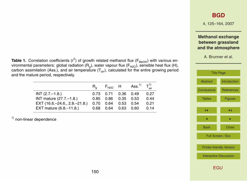
Table 1. Correlation coefficients (r2) of growth related methanol flux (FMeOH) with various en-vironmental parameters: global radiation (Rg), water vapour flux (FH2O), sensible heat flux (H),carbon assimilation (Ass.), and air temperature (Tair), calculated for the entire growing periodand the mature period, respectively.

Rg FH2O H Ass.1) T1)air

INT (2.7.–1.8.) 0.73 0.71 0.36 0.49 0.27INT mature (27.7.–1.8.) 0.85 0.86 0.35 0.53 0.44EXT (16.6.–24.6., 2.8.–21.8.) 0.70 0.64 0.53 0.54 0.21EXT mature (6.8.–11.8.) 0.68 0.64 0.63 0.60 0.14

1) non-linear dependence

150





BGD4, 125–164, 2007


A. Brunner et al.

Title Page



Tables Figures

J I

J I

Back Close

Full Screen / Esc



EGU

Table 2. Characteristics for the intensive and the extensive field during mature phase: 6-daymean of sum (Σ) of global radiation (ΣRg,), air temperature (Tair), rainfall (ΣRain), relative hu-midity (RH), leaf area index (LAI), accumulated daytime (10:00–16:00 LT) carbon assimilation(ΣAss.), and the accumulated methanol emissions (ΣMeOH).

ΣRg Tair ΣRain RH LAI ΣAss. ΣMeOHkW h m−2 ◦C mm % m2 m−2 mgC m−2 mgC m−2

INT 5910 19.5 0 66.2 3.4 39.5 2.8EXT 4140 20.6 30.5 82.6 5.1 42.4 6.3

151





BGD4, 125–164, 2007


A. Brunner et al.

Title Page



Tables Figures

J I

J I

Back Close

Full Screen / Esc



EGU

Table 3. Methanol fluxes measured in field experiments.

Reference Plant species Time of year Fluxes (min–max)mg m−2 h−1

Fukui and Doskey (1998) Grassland Summer ∼ 0.81)

Kirstine et al. (1998) Grass Australian Summer 0.36–0.49Kirstine et al. (1998) White clover Australian Summer 0.03–7.5Baker et al. (2001) Subalpine forest Summer 1999 –0.1–2.5Schade and Goldstein (2001) Ponderosa pine July–September 1999 0.25–1.09Karl et al. (2002) Subalpine forest Summer 2001 0.45–1.05Warneke et al. (2002) Alfalfa field Summer 2000 0–4Das et al. (2003) Maize May 1995 3.45 2)

Karl et al. (2003) Hardwood forest Fall 2001–Summer 2002 0–2Karl et al. (2004) Rain forest 2003 0.13 2)

Karl et al. (2005) Loblolly pine forest July 2003 0.32–0.52 2)

Spirig et al. (2005) Deciduous forest Summer 2003 0–0.31This study Intensive grassland Summer 2004 –0.18–1.11 (0.21 2))This study Extensive grassland Summer 2004 –0.09–2.21 (0.352))

1) Normalized to 25◦C,2) Average fluxes (24h).

152





BGD4, 125–164, 2007


A. Brunner et al.

Title Page



Tables Figures

J I

J I

Back Close

Full Screen / Esc



EGU

Table 4. Accumulated cut- and growth-related methanol emission (CMeOH), net primary produc-tivity (NPP), and harvest yield (CHarvest) of the intensive and the extensive grassland. Growthrelated emissions are referred to the harvest yield of the following cut.

Event/ Date CMeOH CHarvest CMeOH/CHarvest NPP CMeOH/NPPPhase gC m−2 gC m−2 gC m−2

INT Cut 2 25.6.–27.6.04 0.005 138 0.004%Growth 3 28.6.–28.8.04 0.065 81 0.080% 267 0.024%

EXT Cut 1 7.6.–9.6.04 0.028 288 0.010%Growth 2 10.6–28.8.04 0.199 133 0.150% 415 0.048%Cut 2 28.8.–30.8.04 0.007 133 0.005%

153





BGD4, 125–164, 2007


A. Brunner et al.

Title Page



Tables Figures

J I

J I

Back Close

Full Screen / Esc



EGU

Extensive site Intensive site

N

146

m

Anemometer EXTIRGA EXTGas inlet EXT

Meteo station

52 m52 m

A) PTR-MSB) Pump (Flow rate 4 L min-1)C) Anemometer INT, IRGA INT, Gas inlet INTD) PFA tube (30 m)

A)

B)

D)

Monitoringtrailer

C)

Fig. 1. Site sketch: Left: Disposition of the monitoring trailer, the meteo station, the twoanemometers, the two open-path infra-red gas analyzer (IRGA) and the gas inlets above thetwo fields. Right: Measurement arrangement: Gas inlet, pump, and PTR-MS.

154





BGD4, 125–164, 2007


A. Brunner et al.

Title Page



Tables Figures

J I

J I

Back Close

Full Screen / Esc



EGU

-2

0

2

4

6

LAI

m2 / m

2LAI INTLAI EXT

07.06.04 17.06.04 27.06.04 07.07.04 17.07.04 27.07.04 06.08.04 16.08.04 26.08.04 05.09.04

Mea

sure

men

tlo

catio

n

! INT$ EXT

A B

1. EXT

2. INT 3. INT2. EXT

a)

LAI

m2

m-2

EXT

INT

c)

b) Cut

Fig. 2. Field experiment summer 2004, overview on the growing state of the fields, the event-related methanol emission, and the measurements between 7 June and 7 September: (a) LAIof the intensive and the extensive site, (b) cuts of the intensive (25.06 and 28.08.04) and theextensive (07.06 and 28.08.04) site, classification into cut-related (dark-grey bar) and growth-related (light-grey bar) emission periods, and (c) methanol flux sampling scheme. A: maturephase of the intensive site, B: mature phase of the extensive site.

155





BGD4, 125–164, 2007


A. Brunner et al.

Title Page



Tables Figures

J I

J I

Back Close

Full Screen / Esc



EGU

0200400600800

1000

Rg

W m

-2

0

10

20

30

40Te

mp.

C°

Rai

n x

4 m

m

048

2030

F MeO

H

nmol

m-2

s-1

0

10

20

30

40

Ass

.µm

ol m

-2 s

-1

-202468

10

F H2O

mm

ol m

-2 s

-1

26.06.04 03.07.04 10.07.04 17.07.04 24.07.04 31.07.04

05

1015202530

c MeO

Hpp

bv

A

Fig. 3. Time series measured above the intensive grassland (25.06–01.08.2004), from thetop to the bottom: Global radiation* (Rg), air temperature* (Temp.), rainfall*, water vapour flux(FH2O), assimilation (Ass.), methanol flux (FMeOH), and methanol concentration (cMeOH). (A:mature phase of the intensive site). * measured at the meteo station, see Fig. 1.

156





BGD4, 125–164, 2007


A. Brunner et al.

Title Page



Tables Figures

J I

J I

Back Close

Full Screen / Esc



EGU

0 4 9 14 19 0Hour of day

0

10

20

30

INT

c MeO

H

ppbv

MeOH conc.mean MeOH conc

0 4 9 14 19 0Hour of day

0

2.5

5

7.5

u ms-1

0.0 2.5 5.0 7.5ums-1

0

10

20

30

INT

c MeO

H

ppbv

a) b) c)

Fig. 4. Diurnal cycle of (a) methanol concentrations (cMeOH) including hourly mean valuesabove the intensive field, and (b) horizontal wind velocities (u). (c) shows the scatter plotof methanol concentrations vs horizontal wind velocity. The data cover the period 25.06–01.08.2004.

157





BGD4, 125–164, 2007


A. Brunner et al.

Title Page



Tables Figures

J I

J I

Back Close

Full Screen / Esc



EGU

0 200 400 600 800 1000Rg

W m-2

0

4

8

12

F MeO

Hnm

ol m

-2 s

-1

-2 0 2 4 6 8 10FH2O

mmol m-2 s-1

0

4

8

12

5 10 15 20 25 30 35Tair°C

0

4

8

12

5 10 15 20 25 30 35Tair°C

0

4

8

1222.07.04

a) b)

e) f)

-200 -100 0 100 200H

W m-2

0

4

8

12

F MeO

H

nmol

m-2

s-1

c)

0 10 20 30 4

Ass.µmol m-2 s-1

0

-4

0

4

8

12

d)

12:00 LT

08:00 LT

Fig. 5. Scatter plots of methanol flux (FMeOH) vs (a) global radiation (Rg), (b) water vapour flux(FH2O), (c) assimilation (Ass.), (d) sensible heat flux (H), and (e) air temperature (Tair) abovethe intensive field for the period 28.06–01.08.2004. (f) shows the scatter plot of methanol fluxand air temperature for one exemplary day (22.7.2004). The arrow indicates the direction ofthe diurnal course.

158





BGD4, 125–164, 2007


A. Brunner et al.

Title Page



Tables Figures

J I

J I

Back Close

Full Screen / Esc



EGU

0

0.4

0.8

1.2

1.6

2

2.4

γ / L

AInm

ol m

-2 s

-1/ m

mol

m-2

s-1

03.07.04 10.07.04 17.07.04 24.07.04 31.07.04

Aa)

b)

0

0.4

0.8

1.2

1.6

2

2.4

γnm

ol m

-2 s

-1 /

mm

ol m

-2 s

-1

Fig. 6. Time series of (a) γ and (b) γ/LAI of the intensive field. A: mature phase of the intensivefield.

159





BGD4, 125–164, 2007


A. Brunner et al.

Title Page



Tables Figures

J I

J I

Back Close

Full Screen / Esc



EGU

0200400600800

1000

Rg

W m

-2

0

10

20

30

40

Tem

p. C

°R

ain

x 4

mm

-4

0

4

8

12

F H2O

m

mol

m-2

s-1

01020304050

Ass

.µm

ol m

-2 s

-1

05

101520

100120

F MeO

Hnm

ol m

-2 s

-1

12.06.04 22.06.04 11.08.04 21.08.04 31.08.04

01020304050

c MeO

Hpp

bv

B

Fig. 7. Time series measured above the extensive grassland (07.06–07.09.2004), from thetop to the bottom: Global radiation* (Rg), air temperature* (Temp.), rainfall*, water vapour flux(FH2O), assimilation (Ass.), methanol flux (FMeOH), and methanol concentration (cMeOH). (B:mature phase of the extensive site). * measured at the meteo station, see Fig. 1.

160





BGD4, 125–164, 2007


A. Brunner et al.

Title Page



Tables Figures

J I

J I

Back Close

Full Screen / Esc



EGU

0 3 6 9 12 15 18 21 0

Time of the dayh

30405060708090

100110

RH

%

0

2

4

6

8

10

F MeO

H

nmol

m-2

s-1

-2

0

2

4

6

8

10

F H2O

mm

ol m

-2 s

-1

-200

0

200

400

600

800

1000

Rg

W m

-2

0 3 6 9 12 15 18 21 0

Time of the dayh

INT mature EXT mature

a) b)

c) d)

e) f)

g) h)

Fig. 8. Mean hourly values of the mature phase of the intensive (left, +) and the extensivefield (right, ♦ ): (a), (b) methanol flux (FMeOH), (c), (d) water vapour flux (FH2O), (e), (f) globalradiation (Rg), (g), (h) relative humidity (RH). Error bars are the standard deviation.

161





BGD4, 125–164, 2007


A. Brunner et al.

Title Page



Tables Figures

J I

J I

Back Close

Full Screen / Esc



EGU

0 200 400 600 800 1000

Rg

W m-2

0

4

8

12

F MeO

H

nmol

m-2

s-1

EXTINT

0 4 8 12

FH2O mmol m-2 s-1

0

4

8

12

0 10 20 30 4

Ass.µmol m-2 s-1

0

0

4

8

12

0 10 20 30 40

0

4

8

12a) b) c)

Fig. 9. Scatter plots of methanol flux (FMeOH) vs (a) global radiation (Rg), (b) water vapour(FH2O), and (c) assimilation (Ass.) for the mature period of the intensive and the extensivefields (INT: +, EXT: ♦).

162





BGD4, 125–164, 2007


A. Brunner et al.

Title Page



Tables Figures

J I

J I

Back Close

Full Screen / Esc



EGU

0

200

400

600

800

1000

Rg

W m

-2

0

2

4

6

8

10

INT FM

eOH

nmol m

-2 s -1

INT FH

2O m

mol m

-2 s -1

Rg

FH2O

FMeOH

0 2 4 7 9 12 14 16 19 21 0

Hour of the dayh

0

200

400

600

800

1000

Rg

W m

-2

0

2

4

6

8

10

INT FM

eOH

nmol m

-2s -1

INT FH

2O m

mol m

-2 s -1

22.07.04

30.07.04

Fig. 10. Global radiation (Rg), water vapour flux (FH2O), methanol flux (FMeOH) measured abovethe intensive field for the 22.07.04, and the 30.07.04.

163





BGD4, 125–164, 2007


A. Brunner et al.

Title Page



Tables Figures

J I

J I

Back Close

Full Screen / Esc



EGU

03.07.04 10.07.04 17.07.04 24.07.04 31.07.04

-2

0

2

4

6

8

10

F MeO

Hnm

ol m

-2 s

-1

FMeOH mea

FMeOH cal

Fig. 11. Methanol flux (FMeOH) of the intensive field: measured (mea) and calculated (cal) bymean of the multiplicative approach. Correlation between measured and calculated methanolflux of the intensive field (y=0.80x + 0.28; r2=0.79).

164





Documents

Methanol exchange between grassland and the atmosphere - BGD