Meta Analysis

Zhezhen Jin

Department of Biostatistics

Mailman School of Public Health

Columbia University

New York, NY 10032

What is meta-analysis?

Combining information

Evidence based medicine

Pulling together evidence

Systematic reviews

A statistical technique for summarizing the results of several

studies into a single estimate.

A little bit history of meta-analysis

Karl Pearson (1904) Averaged correlations for studies of the

effectiveness of inoculation for typhoid fever

R. A. Fisher (1944) When a number of quite independent tests of

significance have been made, it sometimes happens that although

few or none can be claimed individually as significant, yet the

aggregate gives an impression that the probabilities are on the

whole lower than would often have been obtained by chance Source

of the idea of cumulating probability values

W. G. Cochran (1953) Discusses a method of averaging means

across independent studies Laid-out much of the statistical

foundation that modern meta-analysis is built upon (e.g., inverse

variance weighting and homogeneity testing)

Cochrane Collaboration started in 1993 (Evidence based health

care)

Team work: based on protocol and use summary statistical

techniques

“The Cochrane Collaboration is an international network of more

than 28,000 dedicated people from over 100 countries. We work

together to help healthcare practitioners, policy-makers, patients,

their advocates and carers, make well-informed decisions about

health care, by preparing, updating, and promoting the

accessibility of Cochrane Reviews over 5,000 so far, published

online in the Cochrane Database of Systematic Reviews, part of

The Cochrane Library. We also prepare the largest collection of

records of randomised controlled trials in the world, called

CENTRAL, published as part of The Cochrane Library.”

Driven by the evidence-based medicine movement and the

Cochrane collaboration

Advantages:

Reduces bias

Replicable

Resolves controversy between conflicting findings

Provides reliable basis for decision making

How to perform meta-analysis?

1. Formulate research questions

2. Protocol development

3. Search

4. Study selection (inclusion/exclusion criteria)

5. Quality assessment

6. Data abstraction

7. Analysis

8. Summary

Example: Marfan’s syndrome

It is genetic disorder of the connective tissues

Dominant trait: FBN1

Usually tall, with long limb, leg, thin fingers

Major causes of morbidity and mortality: cardiovascular

complication of aortic dissection and rupture

In late 1960s, blood pressure lowing medication improves survival

of general patients with acute dissection of aortic aneurysms.

With the observation: Blood pressure lowering drug used to treat

patients with aortic root dilatation related to Marfan’s syndrome.

Beta blocker therapy: make heart beats more slowly and with less

force, thereby reducing blood pressure, and also help blood vessels

open up to improve blood flow.

Examples of beta blockers include:

Acebutolol (Sectral)

Atenolol (Tenormin)

Bisoprolol (Zebeta)

Metoprolol

Nadolol (Corgard)

Nebivolol (Bystolic)

Propranolol (Inderal LA)

How much effective the treatment?

Several small studies available, using echocardiography to measure

aortic root dilatation

Clinically, beta-blocker therapy is used routinely for Marfan’s

syndrome patients

Problem: No convincing evidence of long-term outcome.

Meta-analysis was performed.

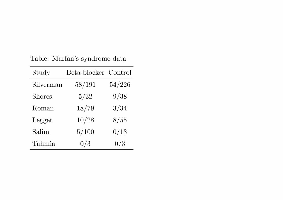
Table: Marfan’s syndrome data

Study Beta-blocker Control

Silverman 58/191 54/226

Shores 5/32 9/38

Roman 18/79 3/34

Legget 10/28 8/55

Salim 5/100 0/13

Tahmia 0/3 0/3

Study types

• Randomized clinical trials

• Observational studies ((e.g. case control, non-randomized

cohorts, cross-sectional prevalence studies, etc.)

• Combination of randomized and observational studies

• Individual patient data studies

Outcome Measures

Create a summary statistic that is comparable across all studies:

1. Binary data: alive/dead, diseased/non-diseased,

Risk difference, relative risk (risk ratio), odds ratio

2. Continuous data: weight loss, blood pressure

Mean difference, standardized mean difference, z-statistic,

p-values

3. Survival data: time to death, time to recurrence, time to

healing

Hazard ratio

4. Ordinal data (ordered categorical data): disease severity,

quality of life

may dichotomize, or treat as continuous

Binary data

Risk difference, relative risk (risk ratio), odds ratio

Table 1. Summary of binary dataRisk difference Relative risk Odds ratio

Parameter D = pT − pC RR = pT /pC OR =pT /(1−pT )pC/(1−pC )

Estimator di = pTi− pCi

ri = pTi/pCi

oi =pTi

/(1−pTi)

pCi/(1−pCi

)

Standard Error sdi=

√pTi

qTinTi

+pCi

qCinCi

slog ri=

√qTi

nTipTi

+qCi

nCipTi

slog oi=

√1a

+ 1b

+ 1c

+ 1d

where qTi = 1− pTi , nTi and nCi de denote the total number of

treated and control patients, and a, b, c, d denote the number of

observations in each cell.

Relative risk and odds ratio both use logarithmic scales

Continuous data

Required for each group: mean, standard deviation, sample size

mean difference, effect size

1. Mean difference: yi = xTi − xCi

Standard error: s2i = s2pi

(1

nTi+ 1

nCi

)where

s2pi=

(nTi − 1)s2Ti+ (nCi − 1)s2Ci

nTi + nCi − 2

2. Effect size (standardized mean difference)

Difference of means divided by the variability of the measures

δ =µT − µC

σ

δ =µT − µC

sp

Survival data

Time to event arise whenever subjects were followed over time until

the event takes place

Problem: not everyone has an event, censoring

Main effect measure: hazard ratio (HR)

HR: ratio of the risk of having an event at any given time in

treatment group over the the risk of an event in the control group.

Analysis with Cox proportional hazards models

Pooling results from different studies

Issues:

Estimates from different studies are different

Two possibilities: sampling error (homogeneous), true variation

exists among studies (heterogeneous)

If homogeneous: fixed effects model

If heterogeneous: random effects model

How to assess heterogeneity?

Cochran’s Chi-square test and I2-test, plots

Test of homogeneity

Suppose there are K studies with summary statistics θi, a

statistical test for the homogeneity

H0 : θ1 = θ2 = · · · = θK = θ

H1 : At least one θi is different

Cochran’s Chi-square test:

Q =K∑i=1

wi(yi − yw)2

where wi = 1/s2i and yw =∑K

i=1 wiyi∑Ki=1 wi

.

Q ∼ χ2K−1, the χ2 distribution with K − 1 degrees of freedom.

Alternatively,

Q =

K∑i=1

wiy2i −

(∑K

i=1 wiyi)2∑K

i=1 wi

Some comments on Cochran’s Q statistic

Power of the test might be very low due to small number of studies

When sample sizes in each study are very large, then H0 may be

rejected even when the individual effect size estimates do not

differ.

The likelihood of design flaws in primary studies and publication

biases makes the interpretation of test complex.

Higgins and Thompson’s I2

I2 = 100(Q− (K − 1))/Q

the proportion of total variability explained by heterogeneity

Values < 25% be thought to be ‘low’

The effect size: has two values, estimate and its standard error

In usual statistics: only one measure is available

Notation: (yi, si), var(yi)=s2i

Idea: yi = θ + ϵi

Fixed effects model and random effects model

Fixed Effects Model

Underlying assumptions:

All studies share common true effect size

Factors that could impact on the true effect size are the same

across studies

Observed effect sizes vary among studies only because a random

sampling error

The random sampling error can be estimated

yi = θ + ϵi

where ϵi ∼ N(0, s2i ) for i = 1, 2, · · · ,K.

The pooled estimate is given by

yw =

∑Ki=1 wiyi∑Ki=1 wi

where wi = 1/s2i .

var(yw) =1∑K

i=1 wi

Approximate 100(1− α)% confidence interval for θ is:

(yw − zα/2√var(yw), yw + zα/2

√var(yw)

Random Effects Model (DerSimonian and Laird model)

Underlying assumptions:

Studies are a random sample of a hypothetical population of

studies.

Two sources of variation: the between and within study variance.

yi = θ + δi + ϵi

where δi ∼ N(0, τ2) and ϵi ∼ N(0, s2i ) for i = 1, 2, · · · ,K. The τ2 is

assumed unknown.

The random effects model will usually generate a confidence

interval as wide or wider than that using the fixed effect model.

Results from a random effects model will usually be more

conservative (there are exceptions).

If τ2 is known, the pooled estimate of θ is given by

θ(τ) =

∑Ki=1 Wi(τ)yi∑Ki=1 Wi(τ)

where Wi(τ) = 1/(s2i + τ2).

var(θ(τ)) =1∑K

i=1 Wi(τ)

Approximate 100(1− α)% confidence interval for θ is:

(θ(τ) − zα/2

√var(θ(τ), θ(τ) + zα/2

√var(θ(τ))

As we said, τ2 is unknown, and need to be estimated.

Under normal error assumptions, maximum likelihood estimate or

restricted maximum likelihood estimate can be used.

Moment based estimate.

τ2 = max

0,Q− (K − 1)∑Ki=1 wi −

∑Ki=1 w2

i∑Ki=1 wi

.

Exploring between study heterogeneity

Random effects models account for heterogeneity between studies,

but fail to explain reasons.

Two approaches can address the issue: subgroup analyses and

meta-regression

Subgroup analyses: focus factors that are possibly different across

studies, such as patient characteristics, study conduct

Meta-regression: include covariates to the fixed and mixed effects

models. Used to estimate the impact/influence of categorical

and/or continuous covariates (moderators) on effect sizes or to

predict effect sizes in studies with specific characteristics. A ratio

of 10:1 (studies to covariates) is recommended

Publication Bias

One major concern of meta-analysis is publication bias:

1. If missing studies are random, failure to include these studies

will result in less information, wider confidence intervals, and

less powerful tests

2. If missing studies are systematically different from available

studies, then results will be biased

Reasons for publication bias:

1. Large studies are likely to be published regardless of statistical

significance

2. Moderately-sized studies are at risk for being lost, only those

with significant results might be published

3. Small studies are at the greatest risk of being lost, studies with

small sample sizes only very large effects are likely to be

significant and those with small and moderate effects are likely

to be unpublished

4. Language bias

How to assess publication bias and how to adjust it?

Funnel plot and linear regression method

Funnel plot: is a scatter plot of sample size or other measure of

precision on the y-axis versus the estimated effect size on the x-axis.

In the absence of publication bias the studies will be distributed

symmetrically about the combined effect size

In the presence of bias, the plot may become skewed, the bottom

of the plot would tend to show a higher concentration of

studies on one side of the mean than the other

This would reflect the fact that smaller studies (which appear

toward the bottom) are more likely to be published if they have

larger than average effects, which makes them more likely to

meet the criterion for statistical significance

Limitations of funnel plot:

It is informal visual method, and a useful funnel plot needs a range

of studies with varying sizes

Different people might interpret the same plot differently

Skewed funnel plot might be caused by factors other than

publication bias

Formal tests

Rank correlation test (Begg and Mazumdar):

y∗i = (yi − yw)/var(yi − yw)

where yw =∑K

i=1 wiyi∑Ki=1 wi

and wi = 1/s2i .

var(yi − yw) = s2i − 1/K∑i=1

wi

Then the rank correlation test is based on statistic

T =K∑i=1

K∑j=1

sign{y∗i − y∗j }

which is U -statistic.

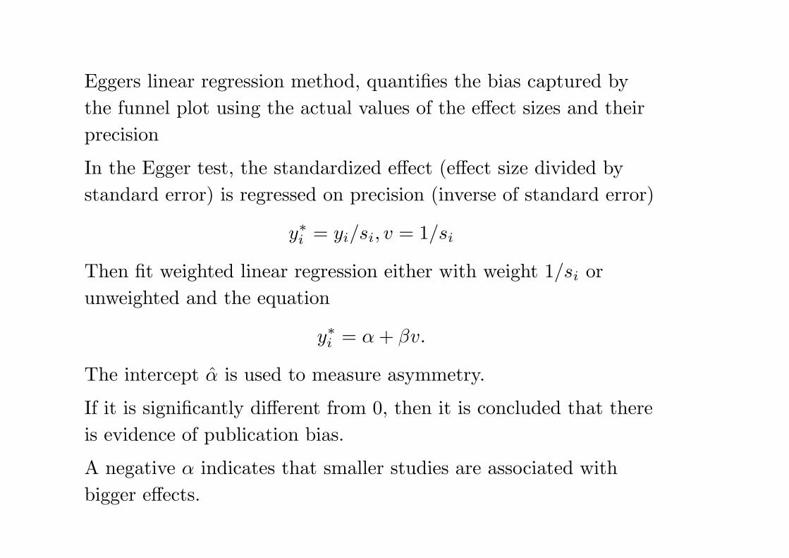
Eggers linear regression method, quantifies the bias captured by

the funnel plot using the actual values of the effect sizes and their

precision

In the Egger test, the standardized effect (effect size divided by

standard error) is regressed on precision (inverse of standard error)

y∗i = yi/si, v = 1/si

Then fit weighted linear regression either with weight 1/si or

unweighted and the equation

y∗i = α+ βv.

The intercept α is used to measure asymmetry.

If it is significantly different from 0, then it is concluded that there

is evidence of publication bias.

A negative α indicates that smaller studies are associated with

bigger effects.

Small studies generally have a precision close to zero, due to their

large standard error In the absence of bias such studies would be

associated with small standardized effects and large studies

associated with large standardized effects

This would create a regression line whose intercept approaches the

origin

If the intercept deviates from this expectation, publication bias

may be the cause

This would occur when small studies are disproportionately

associated with larger effect sizes

If the publication bias is suspected, may model the selection

process into the model for bias correction. One possibility is to

view the problem as a missing data problem and assume that the

studies are missing with probabilities that are a function of their

lack of statistical significance. For example,

pi(z) =

0, if z ≤ 1.96

1, if z > 1.96

Treat pi(z) as missing probability and carry out analysis.

Meta regression

Two types of regression models are possible: fixed effects

meta-regression and random effects mete-regression model

Fixed effects meta-regression:

yi = θ +XTβ + ϵi

where ϵi ∼ N(0, s2i )

Random effects meta-regression:

yi = θ +XTβ + δi + ϵi

where δi ∼ N(0, τ2) and ϵi ∼ N(0, s2i ).

Challenging issues Studies do not report same measures. For

example, the measure for variation might be

Standard errors

Confidence intervals

Reference ranges

Interquartile ranges

Range

Significant test

P-value

‘Not significant’ or ‘P < 0.05’

Number of recurrent events

Number of recurrent events

Individual-patients meta-analysis (recent and still ongoing)

Example: Prevention of fractures after organ transplantation

Organ transplantation: Heart, kidney, lung, liver

Complications: bone loss and fractures

Impact: quality of life

Evidence: 1st year rate 37%

Bone metabolism

Treatment: bisphosphonates, active metabolites of vitamin D

Available studies: small, no definitive clinical trial

To assess differences in bone fracture among treated and untreated

patients.

Data sources and Searches

PUBMED database

MEDLINE database

Cochrane Controlled Clinical Trials Register

Unpublished abstracts for various meetings

Transplant: Kidney, Liver, Heart, Lung

Keywords: transplant, osteoporosis, bone loss, fracture, transplant

and calcitriol, transplant and bisphosphonates, transplant and

osteoporosis, transplant and fracture

Study selection

• Inclusion criteria

Randomized clinical trials, treatment and control groups, fracture

assessment

Age 18 or older

Eligible treatment: oral or IV bisphosphonates (alendronate,

risedronate, pamidronate, ibandronate, zoledronic acid) or active

vitamin D analogs (calcitriol, calcidiol, 1α-hydroxyvitamin D)

No restriction on sample size or specific dose of bisphosphonate or

active vitamin D analog.

• Exclusion criteria

Studies with historical controls were excluded.

Bone marrow transplants were excluded.

Treatments for bone loss prevention: hormone replacement therapy,

calcitonin, or resistence exercise were excluded

Two investigators extracted data on:

Study design, methods, subjects, interventions, fracture, and bone

mineral density (BMD) outcomes.

Primary outcome: vertebral or nonvertebral fracture sustained

within the first year after transplant

Radiographs of the thoracic and lumbar spine (LS) at baseline and

12 months after transplant for fractures

Secondary outcome: BMD measured by dual-energy x-ray

absorptiometry in grams per square centimeter at the LS and

femoral neck (FN)

Quality assessment

Method of randomization, presence/absence of double-blinding,

description of dropouts.

Studies were scored between 0 and 5, with 5 as the highest quality.

685 abstracts: 607 eliminated, 42 duplicate

36 remained, and among them, 28 published

9 were not adequately randomized, 8 were excluded due to delay on

treatment and no response from the authors

Included: 11 studies with 780 participants

Prophylactic use of lidocaine after heart attack

Study Lidocaine Control

1. Chopra 2/39 1/43

2. Mogensen 4/44 4/44

3. Pitt 6/107 4/110

4. Darby 7/103 5/100

5. Bennett 7/110 3/106

6. O’Brian 11/154 4/146

Total 37/557 21/549

Source: Hine, L.K., Laird, N., Hewitt, P. and Chalmers, T.C.

(1989) Meta-analytic evidence against prophylactic use of lidocaine

in Myocardial Infarction, Archives of Internal Medicine, 149,

2694-2698.

RCTs comparing NaF and SMFP

Sodium fuoride (NaF) with sodium monoflouorophosphate (SMFP)

dentrifrices for the purpose of reducing dental decay.

The outcome: decayed, missing or filled teeth score (DMFS)

Study n NaF n SMFP

1 134 5.96 (4.24) 113 6.82 (4.72)

2 175 4.74 (4.64) 151 5.07 (5.38)

3 137 2.04 (2.59) 140 2.51 (3.22)

4 184 2.70 (2.32) 179 3.20 (2.46)

5 174 6.09 (4.86) 169 5.81 (5.14)

6 754 4.72 (5.33) 736 4.76 (5.29)

7 209 10.10 (8.10) 209 10.90 (7.90)

8 1151 2.82 (3.05) 1122 3.01 (3.32)

9 679 3.88 (4.85) 673 4.37 (5.37)

Source: Johnson, M.F. (1993) Comparative efficacy of NaF and

SMFP dentrifrices in caries prevention: a meta-analytic overview,

Caries Res., 27, 328-336.