Embed Size (px)
Citation preview
Show selected photi http://www.admin.technion.ac.il/pard/mediaarc/showphoto.asp?photol...
1 of 1 12/12/08 12:46 PM
Back
Technion logo English
IS
RA
EL
SC
I E N C E F OU
N
DA
TIO
N
School on Interaction of Light with Cold Atoms, Sept. 16-27, 2019, Sao Paulo, Brazil, ICTP-SAIFR/IFT-UNESP.
Eric Akkermans
Based on Mesoscopic physics of electrons and photons, by Eric Akkermans and Gilles Montambaux, Cambridge University Press, 2007
Mesoscopic Physics of Photons

Part 2• Introduction to mesoscopic physics
• The Aharonov-Bohm effect in disordered conductors.• Phase coherence and effect of disorder. • Average coherence: effect and coherent
backscattering.• Phase coherence and self-averaging: universal
fluctuations.• Classical probability and quantum crossings.
�2
Sharvin2
The tools (some of them)

Incoherent propagation !
�3
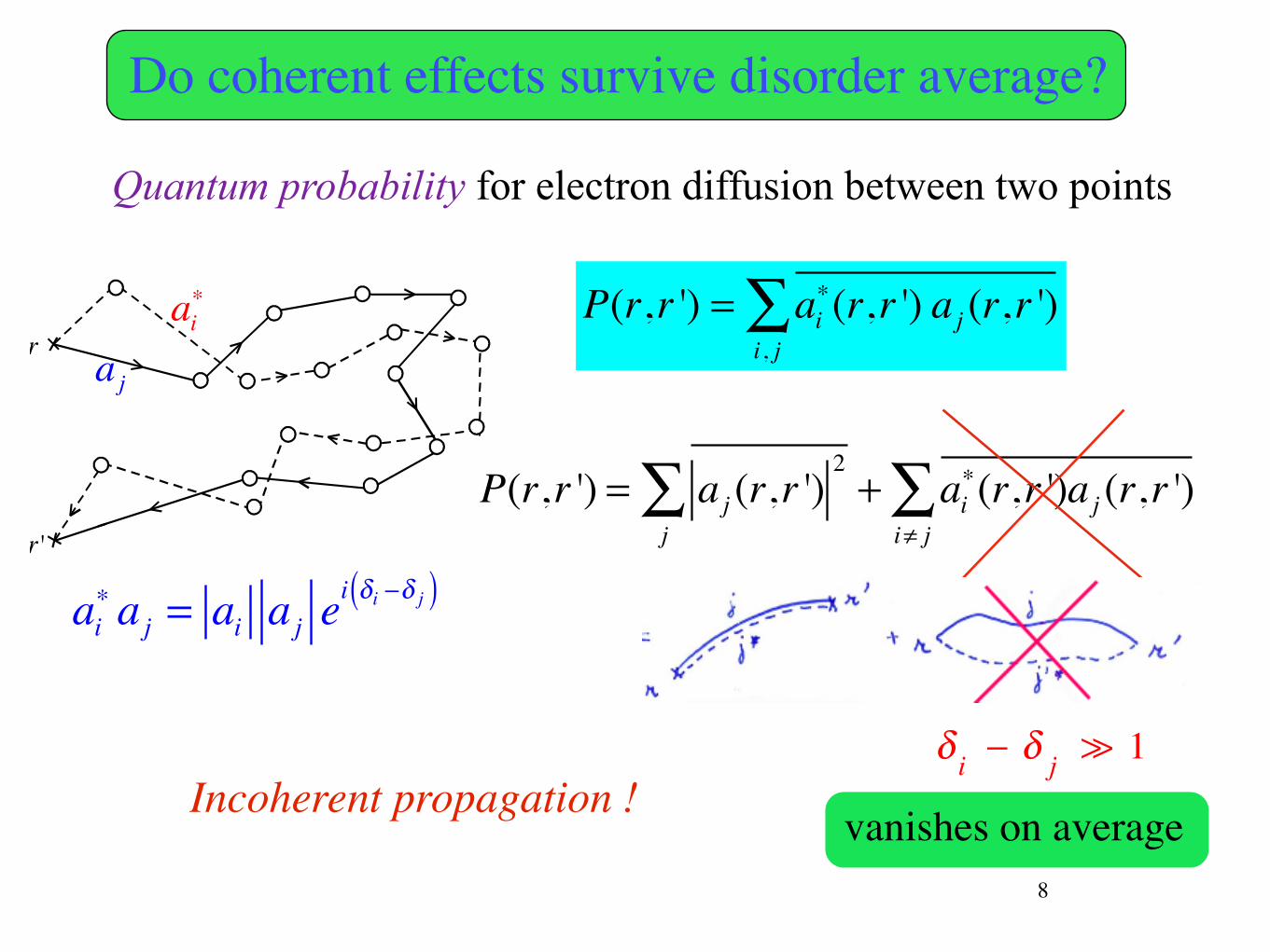
Quantum probability for electron diffusion between two points
P(r,r ') = ai∗(r,r ') aj (r,r ')
i, j∑
r
r'
P(r,r ') = aj (r,r ')2
j∑ + ai
∗(r,r ')aj (r,r ')i≠ j∑
vanishes on average
Do coherent effects survive disorder average?
aj
ai∗
δ i − δ j ≫ 1
ai∗ aj = ai aj e
i δi −δ j( )

Incoherent propagation !
�4
Quantum probability for electron diffusion between two points
P(r,r ') = ai∗(r,r ') aj (r,r ')
i, j∑
r
r'
P(r,r ') = aj (r,r ')2
j∑ + ai
∗(r,r ')aj (r,r ')i≠ j∑
vanishes on average
Do coherent effects survive disorder average?
aj
ai∗
δ i − δ j ≫ 1
ai∗ aj = ai aj e
i δi −δ j( )

Incoherent propagation !
�5
Quantum probability for electron diffusion between two points
P(r,r ') = ai∗(r,r ') aj (r,r ')
i, j∑
r
r'
P(r,r ') = aj (r,r ')2
j∑ + ai
∗(r,r ')aj (r,r ')i≠ j∑
vanishes on average
Do coherent effects survive disorder average?
aj
ai∗
δ i − δ j ≫ 1
ai∗ aj = ai aj e
i δi −δ j( )

Incoherent propagation !
�6
Quantum probability for electron diffusion between two points
P(r,r ') = ai∗(r,r ') aj (r,r ')
i, j∑
r
r'
P(r,r ') = aj (r,r ')2
j∑ + ai
∗(r,r ')aj (r,r ')i≠ j∑
vanishes on average
Do coherent effects survive disorder average?
aj
ai∗
δ i − δ j ≫ 1
ai∗ aj = ai aj e
i δi −δ j( )

Incoherent propagation !
�7
Quantum probability for electron diffusion between two points
P(r,r ') = ai∗(r,r ') aj (r,r ')
i, j∑
r
r'
P(r,r ') = aj (r,r ')2
j∑ + ai
∗(r,r ')aj (r,r ')i≠ j∑
vanishes on average
Do coherent effects survive disorder average?
aj
ai∗
δ i − δ j ≫ 1
ai∗ aj = ai aj e
i δi −δ j( )
Incoherent propagation !
�8
Quantum probability for electron diffusion between two points
P(r,r ') = ai∗(r,r ') aj (r,r ')
i, j∑
r
r'
P(r,r ') = aj (r,r ')2
j∑ + ai
∗(r,r ')aj (r,r ')i≠ j∑
vanishes on average
Do coherent effects survive disorder average?
aj
ai∗
δ i − δ j ≫ 1
ai∗ aj = ai aj e
i δi −δ j( )

aj
ai*r r'
r'r
(a)
(b)
Before averaging : speckle pattern (full coherence)Configuration average: most of the contributions vanish because of large phase differences.
Diffuson Pcl(r, r′) =
!
j
|Aj(r, r′)|2
Ai
A∗
jVanishes upon averaging
Ai
A∗
j
A new design !

aj
ai*r r'
r'r
(a)
(b)
Before averaging : speckle pattern (full coherence)Configuration average: most of the contributions vanish because of large phase differences.
Diffuson Pcl(r, r′) =
!
j
|Aj(r, r′)|2
Ai
A∗
jVanishes upon averaging
Ai
A∗
j
A new design !

aj
ai*r r'
r'r
(a)
(b)
Before averaging : speckle pattern (full coherence)Configuration average: most of the contributions vanish because of large phase differences.
Diffuson Pcl(r, r′) =
!
j
|Aj(r, r′)|2
Ai
A∗
jVanishes upon averaging
Ai
A∗
j
A new design !

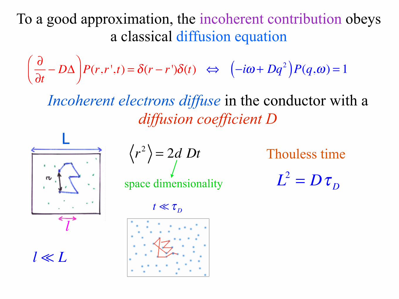
To a good approximation, the incoherent contribution obeys a classical diffusion equation
∂∂t
− DΔ⎛⎝⎜
⎞⎠⎟P(r,r ',t) = δ (r − r ')δ (t)
Incoherent electrons diffuse in the conductor with a diffusion coefficient D
L
l
r2 = 2d Dt
space dimensionality
l ≪ L
L2 = DτD
Thouless time
t ≪ τD t ≫ τD
⇔ −iω + Dq2( )P(q,ω ) = 1
with D =vgl3

To a good approximation, the incoherent contribution obeys a classical diffusion equation
∂∂t
− DΔ⎛⎝⎜
⎞⎠⎟P(r,r ',t) = δ (r − r ')δ (t)
Incoherent electrons diffuse in the conductor with a diffusion coefficient D
L
l
r2 = 2d Dt
space dimensionality
l ≪ L
L2 = DτD
Thouless time
t ≪ τD t ≫ τD
⇔ −iω + Dq2( )P(q,ω ) = 1
t
τe τD
τφ
ballistic
diffusive ergodic
mesoscopic limit classical limit

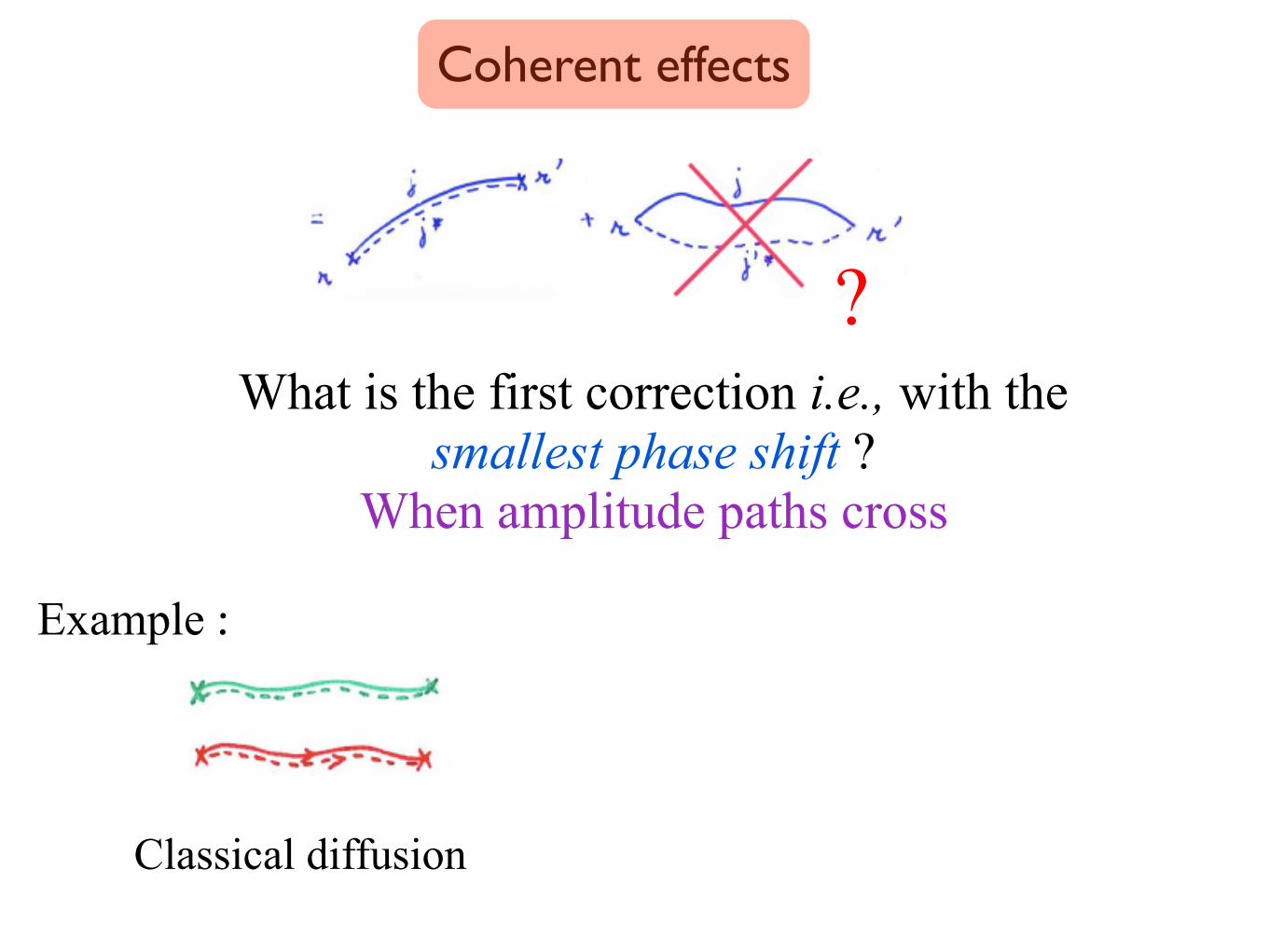
?What is the first correction i.e., with the
smallest phase shift ? When amplitude paths cross
Example :
Classical diffusion
quantum crossing
Exchange of amplitudes
Coherent effects

?What is the first correction i.e., with the
smallest phase shift ? When amplitude paths cross
Example :
Classical diffusion
quantum crossing
Exchange of amplitudes
Coherent effects
?What is the first correction i.e., with the
smallest phase shift ? When amplitude paths cross
Example :
Classical diffusion
quantum crossing
Exchange of amplitudes
Coherent effects

?What is the first correction i.e., with the
smallest phase shift ? When amplitude paths cross
Example :
Classical diffusion
quantum crossing
Exchange of amplitudes
Coherent effects

Occurrence of a quantum crossing after a time t for a photon diffusing in a volume Ld
p× (t) =λd−1ctLd
The time spent by a diffusing photon is so that τD = L2
D
p× (τD ) =λd−1cτDLd
≡1g
g = Dcλ d−1 L
d−2

Occurrence of a quantum crossing after a time t for a photon diffusing in a volume Ld
p× (t) =λd−1ctLd
The time spent by a diffusing photon is so that τD = L2
D
p× (τD ) =λd−1cτDLd
≡1g
g = Dcλ d−1 L
d−2

Occurrence of a quantum crossing after a time t for a photon diffusing in a volume Ld
p× (t) =λd−1ctLd
The time spent by a diffusing photon is so that τD = L2
D
p× (τD ) =λd−1cτDLd
≡1g
g = Dcλ d−1 L
d−2

Occurrence of a quantum crossing after a time t for a photon diffusing in a volume Ld
p× (t) =λd−1ctLd
The time spent by a diffusing photon is so that τD = L2
D
p× (τD ) =λd−1cτDLd
≡1g
g = Dcλ d−1 L
d−2

λd−1 lVolume
Quantum crossings decrease the diffusion coefficient D : weak localization
λ : wavelength

Physical meaning of this parameter ?
g = Dcλ d−1 L
d−2

A metal can be modeled as a quantum gas of electrons scattered by an elastic disorder.
Classically, the conductance of a cubic sample of size is given by Ohm’s law: where is the conductivity. G = σL
d−2
Ld
σ
g =le
3λd−1Ld−2 = Gcl/(e2/h)
is the classical electrical conductance so that
Gcl/(e2/h) ≫ 1
Gcl
Electrical conductance of a metal
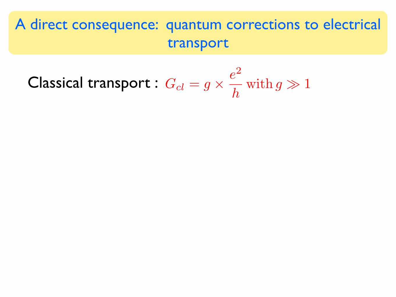
Classical transport : Gcl = g ×e2
hwith g ≫ 1
Quantum corrections: ∆G = Gcl ×1
g
so that ∆G ≃
e2
h
A direct consequence: quantum corrections to electrical transport

Classical transport : Gcl = g ×e2
hwith g ≫ 1
Quantum corrections: ∆G = Gcl ×1
g
so that ∆G ≃
e2
h
A direct consequence: quantum corrections to electrical transport

Classical transport : Gcl = g ×e2
hwith g ≫ 1
Quantum corrections: ∆G = Gcl ×1
g
A direct consequence: quantum corrections to electrical transport
so that is universal∆G ≃
e2
h
Independent of the microscopic (and often unknown) disorder - Depends only on the geometry

Classical transport : Gcl = g ×e2
hwith g ≫ 1
Quantum corrections: ∆G = Gcl ×1
g
A direct consequence: quantum corrections to electrical transport
so that is universal#
Not that simple ! We wish to obtain precise
numbers... Need to sum up Feynman diagrams.

Classical transport : Gcl = g ×e2
hwith g ≫ 1
Quantum corrections: ∆G = Gcl ×1
g
A direct consequence: quantum corrections to electrical transport
so that is universal#
Not that simple ! We wish to obtain precise
numbers... Need to sum up Feynman diagrams.
+= +
= + +
==
=
b) diffusion anisotrope
a) diffusion isotrope
c) =
+= +
= + +
==
=
b) diffusion anisotrope
a) diffusion isotrope
c) =
(a) (b) (c)
(d) (e)
(d) (e)

An intermezzo based on our understanding of coherent effects

�41
Expansion in powers of quantum crossings allows to calculate quantum corrections to physical quantities.
This singular perturbation expansion is not a simple coincidence but an expression of scaling
A renormalization of D(L) changes also g(L):
1 g
The diffusion coefficient D is reduced (weak localization) and becomes size dependent :
g(L) = D(L)cλd−1 L
d−2 ≈N⊥2 (L)N
A quantum phase transition: Anderson localization
D(L) = D 1− 1πgln L
l( ) + 1πgln L
l( )⎛⎝⎜
⎞⎠⎟
2
+ ....⎛
⎝⎜
⎞
⎠⎟ (d = 2)

�42
Expansion in powers of quantum crossings allows to calculate quantum corrections to physical quantities.
This singular perturbation expansion is not a simple coincidence but an expression of scaling
A renormalization of D(L) changes also g(L):
1 g
The diffusion coefficient D is reduced (weak localization) and becomes size dependent :
g(L) = D(L)cλd−1 L
d−2 ≈N⊥2 (L)N
A quantum phase transition: Anderson localization
D(L) = D 1− 1πgln L
l( ) + 1πgln L
l( )⎛⎝⎜
⎞⎠⎟
2
+ ....⎛
⎝⎜
⎞
⎠⎟ (d = 2)

�43
Expansion in powers of quantum crossings allows to calculate quantum corrections to physical quantities.
This singular perturbation expansion is not a simple coincidence but an expression of scaling
A renormalization of D(L) changes also g(L):
1 g
The diffusion coefficient D is reduced (weak localization) and becomes size dependent :
g(L) = D(L)cλd−1 L
d−2 ≈N⊥2 (L)N
A quantum phase transition: Anderson localization
D(L) = D 1− 1πgln L
l( ) + 1πgln L
l( )⎛⎝⎜
⎞⎠⎟
2
+ ....⎛
⎝⎜
⎞
⎠⎟ (d = 2)

�44
Expansion in powers of quantum crossings allows to calculate quantum corrections to physical quantities.
This singular perturbation expansion is not a simple coincidence but an expression of scaling
A renormalization of D(L) changes also g(L):
1 g
The diffusion coefficient D is reduced (weak localization) and becomes size dependent :
g(L) = D(L)cλd−1 L
d−2 ≈N⊥2 (L)N
A quantum phase transition: Anderson localization
D(L) = D 1− 1πgln L
l( ) + 1πgln L
l( )⎛⎝⎜
⎞⎠⎟
2
+ ....⎛
⎝⎜
⎞
⎠⎟ (d = 2)

�45
Expansion in powers of quantum crossings allows to calculate quantum corrections to physical quantities.
This singular perturbation expansion is not a simple coincidence but an expression of scaling
A renormalization of D(L) changes also g(L):
1 g
The diffusion coefficient D is reduced (weak localization) and becomes size dependent :
g(L) = D(L)cλd−1 L
d−2 ≈N⊥2 (L)N
A quantum phase transition: Anderson localization
D(L) = D 1− 1πgln L
l( ) + 1πgln L
l( )⎛⎝⎜
⎞⎠⎟
2
+ ....⎛
⎝⎜
⎞
⎠⎟ (d = 2)

�46
Scaling and its meaning :
If we know , we know it at any scale :
g (L(1 + ϵ)) = g(L)!
1 + ϵβ(g) + O(g−5)"
β(g) =d ln g
d lnL
Expanding, we have
with (Gell-Mann - Low function)
Scaling behavior :
(P.W. Anderson et al.,1979)
g(L)
g L(1+ ε)( )= f g(L),ε( )
ξ(W ) is the localization length
g(L,W ) = f Lξ(W )( )

�47
Scaling and its meaning :
If we know , we know it at any scale :
g (L(1 + ϵ)) = g(L)!
1 + ϵβ(g) + O(g−5)"
β(g) =d ln g
d lnL
Expanding, we have
with (Gell-Mann - Low function)
Scaling behavior :
(P.W. Anderson et al.,1979)
g(L)
g L(1+ ε)( )= f g(L),ε( )
ξ(W ) is the localization length
g(L,W ) = f Lξ(W )( )

�48
Scaling and its meaning :
If we know , we know it at any scale :
g (L(1 + ϵ)) = g(L)!
1 + ϵβ(g) + O(g−5)"
β(g) =d ln g
d lnL
Expanding, we have
with (Gell-Mann - Low function)
Scaling behavior :
(P.W. Anderson et al.,1979)
g(L)
g L(1+ ε)( )= f g(L),ε( )
ξ(W ) is the localization length
g(L,W ) = f Lξ(W )( )

�49
Scaling and its meaning :
If we know , we know it at any scale :
g (L(1 + ϵ)) = g(L)!
1 + ϵβ(g) + O(g−5)"
β(g) =d ln g
d lnL
Expanding, we have
with (Gell-Mann - Low function)
Scaling behavior :
(P.W. Anderson et al.,1979)
g(L)
g L(1+ ε)( )= f g(L),ε( )
ξ(W ) is the localization length
g(L,W ) = f Lξ(W )( )

g(L,W )
Lξ(W )
d = 3
Anderson phase transition
d = 2
B.Kramer, A. McKinnon, 1981
Anderson localization phase transition occurs in d > 2
Numerical calculations on the (universal) Anderson Hamiltonian

End of the intermezzo based on our understanding of coherent effects

Weak disorder limit:
Probability of a crossing is small: phase coherent corrections to the classical limit are small.
Quantum crossings modify the classical probability (i.e. the Diffuson). Due to its long range behavior, the Diffuson propagates (localized) coherent effects over large distances.
Weak disorder physics
Quantum crossings are independently distributed : We can generate higher order corrections to the Diffuson as an expansion in powers of 1 / g
∝1 g( )
λ<< l ⇒ g >> 1

Weak disorder limit:
Probability of a crossing is small: phase coherent corrections to the classical limit are small.
Quantum crossings modify the classical probability (i.e. the Diffuson). Due to its long range behaviour, the Diffuson propagates (localized) coherent effects over large distances.
Weak disorder physics
Quantum crossings are independently distributed : We can generate higher order corrections to the Diffuson as an expansion in powers of 1 / g
∝1 g( )
λ<< l ⇒ g >> 1

To the classical probability corresponds the Drude conductance Gcl
First correction involves one quantum crossing and the probability to have a closed loop:
(∝1 / g)
Return probability
quantum correction decreases the conductance: weak localization
L
Weak localization- Electronic transport
τD = L2 D
Z(t) =
!
drPint(r, r, t) =" τD
4πt
#d/2
�
po (τD )
�
ΔGGcl
=− po (τD )
�
po (τD ) =1g
Z(t) dtτD0
τ D
∫

|A(k,k′)|2 =!
r1,r2
|f(r1, r2)|2"
1 + ei(k+k′).(r1−r2)#
Generally, the interference term vanishes due to the sum over , except for two notable cases:r1 and r2
k + k′≃ 0 : Coherent backscattering
r1 − r2 ≃ 0 : closed loops, weak localization and periodicity of the Sharvin effect.
φ0/2
-100 0 100 200 300
0.8
1.2
1.6
2.0
Scal
ed In
tens
ity
Angle (mrad)
-5 0 51.8
1.9
2.0
Coherent backscattering
A reminder !

|A(k,k′)|2 =!
r1,r2
|f(r1, r2)|2"
1 + ei(k+k′).(r1−r2)#
Generally, the interference term vanishes due to the sum over , except for two notable cases:r1 and r2
k + k′≃ 0 : Coherent backscattering
r1 − r2 ≃ 0 : closed loops, weak localization and periodicity of the Sharvin effect.
φ0/2
-100 0 100 200 300
0.8
1.2
1.6
2.0
Scal
ed In
tens
ity
Angle (mrad)
-5 0 51.8
1.9
2.0
Coherent backscattering

|A(k,k′)|2 =!
r1,r2
|f(r1, r2)|2"
1 + ei(k+k′).(r1−r2)#
Generally, the interference term vanishes due to the sum over , except for two notable cases:r1 and r2
k + k′≃ 0 : Coherent backscattering
r1 − r2 ≃ 0 : closed loops, weak localization and periodicity of the Sharvin effect.
φ0/2
this case


In the presence of a dephasing mechanism that breaks time coherence, only trajectories with contribute.
In the presence of an Aharonov-Bohm flux, paired amplitudes in the Cooperon acquire opposite phases:
φ2πφ/φ0 −2πφ/φ0 the phase difference becomes: 4πφ/φ0
t < τφ
Cooperon
φ0/2 periodicity of the Sharvin effect
is obtained from the covariant diffusion equationPint(r, r′, t)
!
1
τφ+
∂
∂t− D
"
∇r′ + i2e
hA(r′)
#2$
Pint(r, r′, t) = δ(r − r′)δ(t)
effective charge 2e


Back to coherent effects for light

An analogous problem: Speckle patterns in opticsConsider the elastic multiple scattering of light transmitted through a fixed disorder configuration.
Outgoing light builds a speckle pattern i.e., an interference picture:L
saa sb
sa' sb'

An analogous problem: Speckle patterns in opticsConsider the elastic multiple scattering of light transmitted through a fixed disorder configuration.
Outgoing light builds a speckle pattern i.e., an interference picture:L
saa sb
sa' sb'

Elastic disorder is not related to decoherence : disorder does not destroy phase coherence and does not introduce irreversibility.
What about speckle patterns ?
Averaging over disorder does not produce incoherent intensity only, but also an angular dependent part, the coherent backscattering, which is a coherence effect. We may conclude:

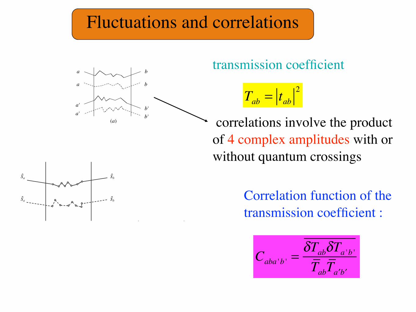
Tab = tab2
Caba 'b ' =δTabδTa 'b 'TabT ′a ′b
Slab geometry
transmission coefficient
Correlation function of the transmission coefficient :
correlations involve the product of 4 complex amplitudes with or without quantum crossingsa
a
a'a'
bb
b'
(b)
b'
b'
a
a
a'
(c)
a'
b
b
b'
(a)
(d) (e)
aa
a'a'
b'
b
b'
b
a
a
a'a'
b
b
b'b'
+
+
aa
a'a'
b
b
b'
b'
Fluctuations and correlations
Slab geometry
L
saa sb
sa' sb'

Tab = tab2
Caba 'b ' =δTabδTa 'b 'TabT ′a ′b
Slab geometry
transmission coefficient
Correlation function of the transmission coefficient :
correlations involve the product of 4 complex amplitudes with or without quantum crossingsa
a
a'a'
bb
b'
(b)
b'
b'
a
a
a'
(c)
a'
b
b
b'
(a)
(d) (e)
aa
a'a'
b'
b
b'
b
a
a
a'a'
b
b
b'b'
+
+
aa
a'a'
b
b
b'
b'
Fluctuations and correlations
12.3 Average transmission coefficient 433
the following sections, we evaluate these various contributions, corresponding respectivelyto zero, one and two crossings.
12.3 Average transmission coefficient
In order to calculate the average of the transmission and reflection coefficients, we use thediffusion approximation to calculate the product of amplitudes depicted in Figure 12.7. Inreflection, the average outgoing intensity is given by (8.6), and the reflection coefficientis given by the albedo (8.13) (see Exercise 8.2 for the slab geometry). For the averagetransmission coefficient, we obtain an analogous relation,5 namely
T ab = 4πR2
cI0S
!dr1 dr2 |ψa(r1)|2#(r1, r2)|GR
(r2, r)|2 (12.12)
where #(r1, r2) is the structure factor taken at zero frequency, and ψa(r1) accounts foran incident plane wave attenuated over the elastic mean free path while entering into thescattering medium (relation 8.7):
ψa(r1) ="
cI0
4πe−|r1−r|/2le eik sa ·r1 . (12.13)
r is a point on the interface (Figure 12.7(b)). The average Green function GR(r2, R)
accounts for the propagation of the wave between the last scattering event up to a pointR far away from the scattering medium. In this so-called Fraunhoffer limit (relation 8.9),we have
GR(r2, R) = e−|r′−r2|/2le e−ik sb·r2
eikR
4πR, (12.14)
r1 r2
r'r
(a) (b)
sa
sa
sa
sb
sb
sb
Figure 12.7 Schematic representation (a) of the product of two amplitudes ψ corresponding to twoincident plane waves along the directions sa emergent along sb, (b) of the Diffuson that results from thepairing of these two amplitudes and that represents the main contribution to the average transmissioncoefficient Tab. r and r′ are points on the interface plane whereas (r1, r2) are the extremities of amultiple scattering trajectory.
5 We assume that the difference in refraction index between the two media is negligible.

Tab = tab2
Caba 'b ' =δTabδTa 'b 'TabT ′a ′b
Slab geometry
transmission coefficient
Correlation function of the transmission coefficient :
correlations involve the product of 4 complex amplitudes with or without quantum crossingsa
a
a'a'
bb
b'
(b)
b'
b'
a
a
a'
(c)
a'
b
b
b'
(a)
(d) (e)
aa
a'a'
b'
b
b'
b
a
a
a'a'
b
b
b'b'
+
+
aa
a'a'
b
b
b'
b'
Fluctuations and correlations

Tab = tab2
Caba 'b ' =δTabδTa 'b 'TabT ′a ′b
transmission coefficient
Correlation function of the transmission coefficient :
Fluctuations and correlations
430 Correlations of speckle patterns
(a)
ab a
ab
(b)
a' b'
(c) (d)
Figure 12.3 Schematic representation of the various setups designed for measurement of thecorrelations of the transmission coefficients: (a) transmission coefficient Tab, (b) correlation functionCaba′b′ , (c) transmission coefficient Ta for an incident plane wave sa obtained by integration overall emergent directions, (d) transmission coefficient T obtained by integration over all incident andemergent directions.
These various quantities are represented schematically in Figure 12.3. As we shall see,this is the total transmission coefficient T that will play a role analogous to the electricalconductance. This is the physical content of the Landauer formula (7.141).
Just like electrical conductance fluctuations, the correlation function δTabδTa′b′ involvesthe disorder average of a product of four amplitudes. In order to exhibit the variouscontributions to this correlation function, we follow the strategy developed in section 9.2.The complex scattering amplitude (12.3) takes the form
ψab ∝!
dr dr′ eik(sa ·r−sb·r′)"
CEC , (12.7)
where the amplitude EC corresponds to a given multiple scattering trajectory C. We thusobtain for the correlation function the average product
"
C1,C2,C3,C4
Ea,bC1
E∗a,bC2
Ea′,b′C3
E∗a′,b′C4
, (12.8)
where the notation used is defined in Figure 12.4. The non-vanishing contributions to thisaverage value of four amplitudes involve two Diffusons. We thus retain in the summation(12.8) the two terms such that C1 = C2 and C3 = C4, or C1 = C4 and C3 = C2. Thesetwo combinations of amplitudes are depicted schematically in Figure 12.5. The first isnothing but the product of the average values of the transmission coefficient. The secondcombination gives
δTabδTa′b′(1) =
#4πR2
cSI0
$2 %%%ψabψ∗a′b′
%%%2
(12.9)
and the corresponding term in the correlation function Caba′b′ is denoted by C(1)aba′b′ . For the
specific combination a = a′ and b = b′, which corresponds to a speckle pattern generated
Measure different configurations

438 Correlations of speckle patterns
(c)
(b)
(a)
Figure 12.8 Right: speckle patterns measured in transmission for different directions of the incidentbeam. The arrow is a guide to show the evolution of a particular feature. The first picture is the referencepattern, corresponding to a given direction of the incident beam. By slowly tilting the incident beam(10 mdeg, then 20 mdeg), we notice a corresponding shift of the speckle pattern which retains some“memory” of the reference pattern. If the tilt angle becomes too large, the speckle is distorted. Left:corresponding behavior of the correlation Caba′b′ as a function of the angle !sb. The upper curve (a)is the autocorrelation (i.e., for a = a′) of the reference speckle pattern. The width is of order 1/kW .The two other figures (b, c) display the correlation of the second and of the third speckle patterns withthe reference pattern (i.e., a = a′). The correlation is maximum for !sb = !sa , and this maximumis F1(kL|!sa|). It vanishes for angles larger than |!sa| ≃ 1/kL [303].
Exercise 12.1: correlation of a speckle pattern measured in reflectionWe denote by Rab the reflection coefficient (i.e., the albedo defined in Chapter 8).Using a modification of (12.22), show that the angular correlation of Rab is
δRabδRa′b′ =!
1
(4π)2S
"dr1 dr2 eik[!sa ·r1 − !sb·r2] e − z1/le e − z2/le $(r1, r2)
#2(12.35)
or equivalently,
δRabδRa′b′ = δ!sa ,!sb
!c
4π l2e
" ∞
0dz1 dz2 e − z1/le e − z2/le Pd (qa , z1, z2)
#2(12.36)
with qa = k|!sa|.

Tab = tab2
Caba 'b ' =δTabδTa 'b 'TabT ′a ′b
transmission coefficient
Correlation function of the transmission coefficient :
Fluctuations and correlations
430 Correlations of speckle patterns
(a)
ab a
ab
(b)
a' b'
(c) (d)
Figure 12.3 Schematic representation of the various setups designed for measurement of thecorrelations of the transmission coefficients: (a) transmission coefficient Tab, (b) correlation functionCaba′b′ , (c) transmission coefficient Ta for an incident plane wave sa obtained by integration overall emergent directions, (d) transmission coefficient T obtained by integration over all incident andemergent directions.
These various quantities are represented schematically in Figure 12.3. As we shall see,this is the total transmission coefficient T that will play a role analogous to the electricalconductance. This is the physical content of the Landauer formula (7.141).
Just like electrical conductance fluctuations, the correlation function δTabδTa′b′ involvesthe disorder average of a product of four amplitudes. In order to exhibit the variouscontributions to this correlation function, we follow the strategy developed in section 9.2.The complex scattering amplitude (12.3) takes the form
ψab ∝!
dr dr′ eik(sa ·r−sb·r′)"
CEC , (12.7)
where the amplitude EC corresponds to a given multiple scattering trajectory C. We thusobtain for the correlation function the average product
"
C1,C2,C3,C4
Ea,bC1
E∗a,bC2
Ea′,b′C3
E∗a′,b′C4
, (12.8)
where the notation used is defined in Figure 12.4. The non-vanishing contributions to thisaverage value of four amplitudes involve two Diffusons. We thus retain in the summation(12.8) the two terms such that C1 = C2 and C3 = C4, or C1 = C4 and C3 = C2. Thesetwo combinations of amplitudes are depicted schematically in Figure 12.5. The first isnothing but the product of the average values of the transmission coefficient. The secondcombination gives
δTabδTa′b′(1) =
#4πR2
cSI0
$2 %%%ψabψ∗a′b′
%%%2
(12.9)
and the corresponding term in the correlation function Caba′b′ is denoted by C(1)aba′b′ . For the
specific combination a = a′ and b = b′, which corresponds to a speckle pattern generated
Measure different configurations

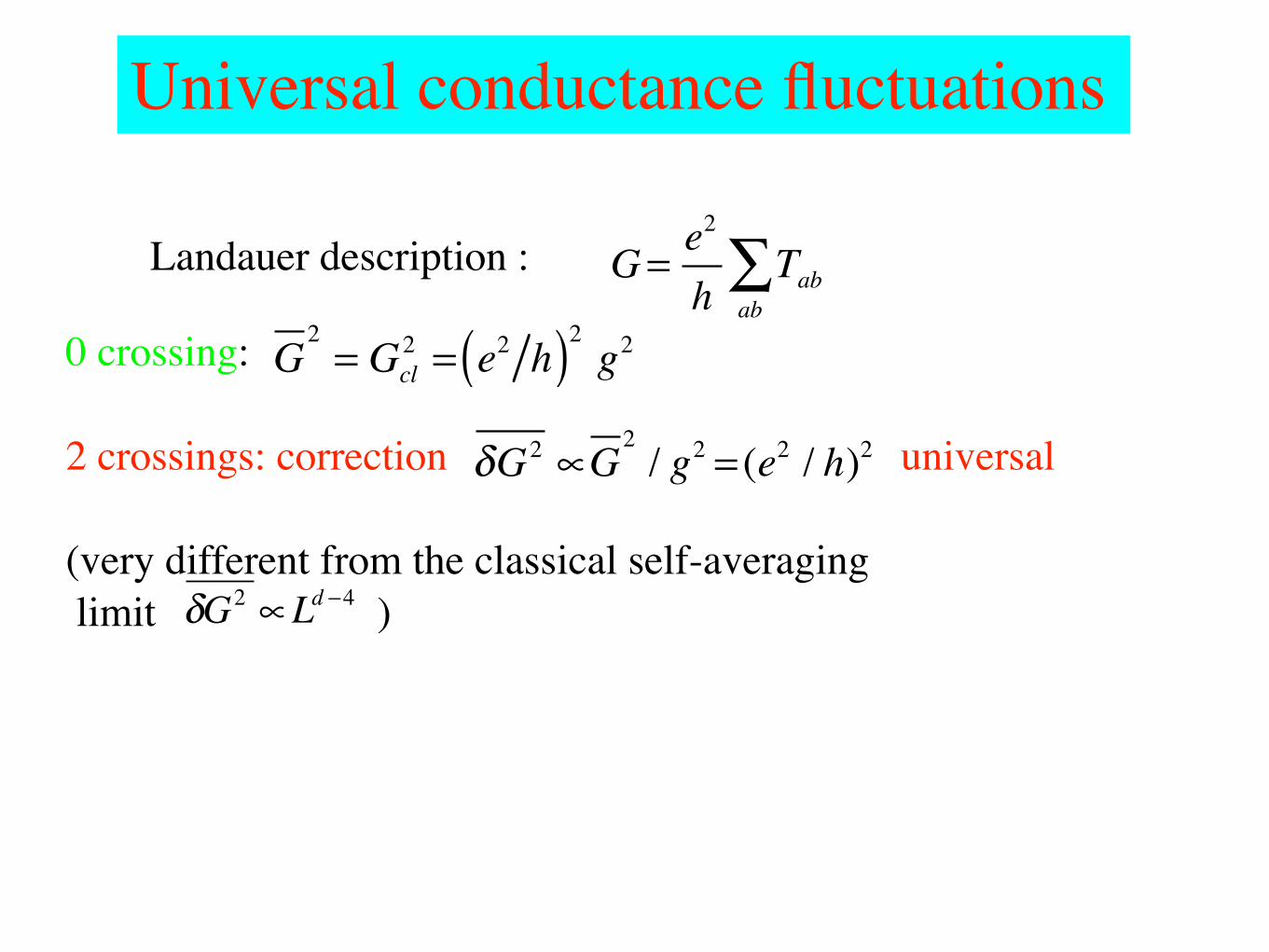
Universal conductance fluctuations
0 crossing: 1 crossing: vanishes due to the summation over the channels.2 crossings: correction universal
(very different from the classical self-averaging limit )
G2= Gcl
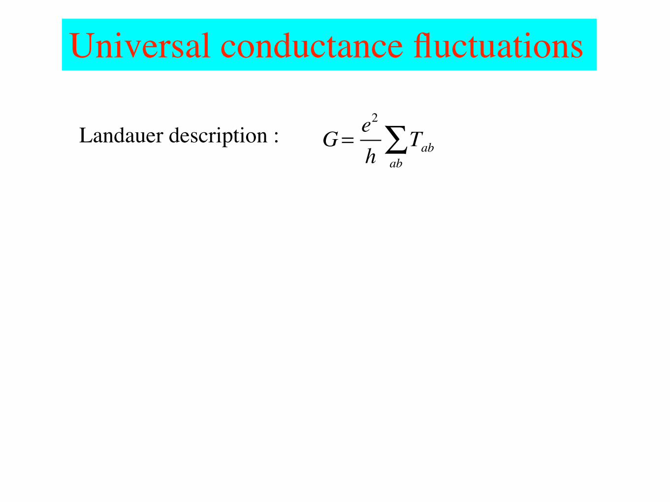
2 = e2 h( )2 g2Landauer description : G=
e2
hTab
ab∑
δG2 ∝G2/ g2 = (e2 / h)2
�
δG2 ∝Ld −4

Universal conductance fluctuations
0 crossing: 1 crossing: vanishes due to the summation over the channels.2 crossings: correction universal
(very different from the classical self-averaging limit )
G2= Gcl
2 = e2 h( )2 g2Landauer description : G=
e2
hTab
ab∑
δG2 ∝G2/ g2 = (e2 / h)2
�
δG2 ∝Ld −4

Universal conductance fluctuations
0 crossing: 1 crossing: vanishes due to the summation over the channels.2 crossings: correction universal
(very different from the classical self-averaging limit )
G2= Gcl
2 = e2 h( )2 g2Landauer description : G=
e2
hTab
ab∑
δG2 ∝G2/ g2 = (e2 / h)2
�
δG2 ∝Ld −4
Universal conductance fluctuations
0 crossing: 1 crossing: vanishes due to the summation over the channels.2 crossings: correction universal
(very different from the classical self-averaging limit )
G2= Gcl
2 = e2 h( )2 g2Landauer description : G=
e2
hTab
ab∑
δG2 ∝G2/ g2 = (e2 / h)2
�
δG2 ∝Ld −4

Universal conductance fluctuations
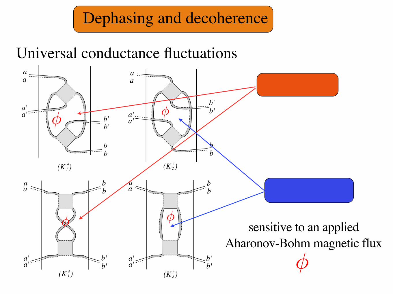
Dephasing and decoherence
aa
bb
a'a' b'
b'
(K )1
aa
bb
b'b'a'
a'
(K )2
aa
a'a'
bb
b'b'
(K )d3
aa
a'a'
bb
b'b'
(K )c3
cd
2 Diffusons
2 Cooperons
sensitive to an applied Aharonov-Bohm magnetic flux
φ
φ φ
φ
φ
Different contributions either sensitive or not to dephasing

k
k'
r1
rb
ry
r2
ra
rz
k
k'
r1
rb
ry
r2
ra
rz
(b)
(a)
r1 → ra → rb · · · → ry → rz → r2
r2 → rz → ry · · · → rb → ra → r1
The total average intensity is:
|A(k,k′)|2 =!
r1,r2
|f(r1, r2)|2"
1 + ei(k+k′).(r1−r2)#
incoherent classical term
interference term
Reciprocity theorem: If I see you, then you see me.
A reminder !

k
k'
r1
rb
ry
r2
ra
rz
k
k'
r1
rb
ry
r2
ra
rz
(b)
(a)
r1 → ra → rb · · · → ry → rz → r2
r2 → rz → ry · · · → rb → ra → r1
The total average intensity is:
|A(k,k′)|2 =!
r1,r2
|f(r1, r2)|2"
1 + ei(k+k′).(r1−r2)#
incoherent classical term
interference term
Reciprocity theorem: If I see you, then you see me.

In the presence of a dephasing mechanism that breaks time coherence, only trajectories with contribute.
In the presence of an Aharonov-Bohm flux, paired amplitudes in the Cooperon acquire opposite phases:
φ2πφ/φ0 −2πφ/φ0 the phase difference becomes: 4πφ/φ0
t < τφ
Cooperon
φ0/2 periodicity of the Sharvin effect
is obtained from the covariant diffusion equationPint(r, r′, t)
!
1
τφ+
∂
∂t− D
"
∇r′ + i2e
hA(r′)
#2$
Pint(r, r′, t) = δ(r − r′)δ(t)
effective charge 2e A reminder !

Universal conductance fluctuations
Dephasing and decoherence
aa
bb
a'a' b'
b'
(K )1
aa
bb
b'b'a'
a'
(K )2
aa
a'a'
bb
b'b'
(K )d3
aa
a'a'
bb
b'b'
(K )c3
cd
Universal conductance fluctuations
Dephasing and decoherence
aa
bb
a'a' b'
b'
(K )1
aa
bb
b'b'a'
a'
(K )2
aa
a'a'
bb
b'b'
(K )d3
aa
a'a'
bb
b'b'
(K )c3
cd
2 Diffusons
2 Cooperons
sensitive to an applied Aharonov-Bohm magnetic flux
φ
φ φ
φ
φ

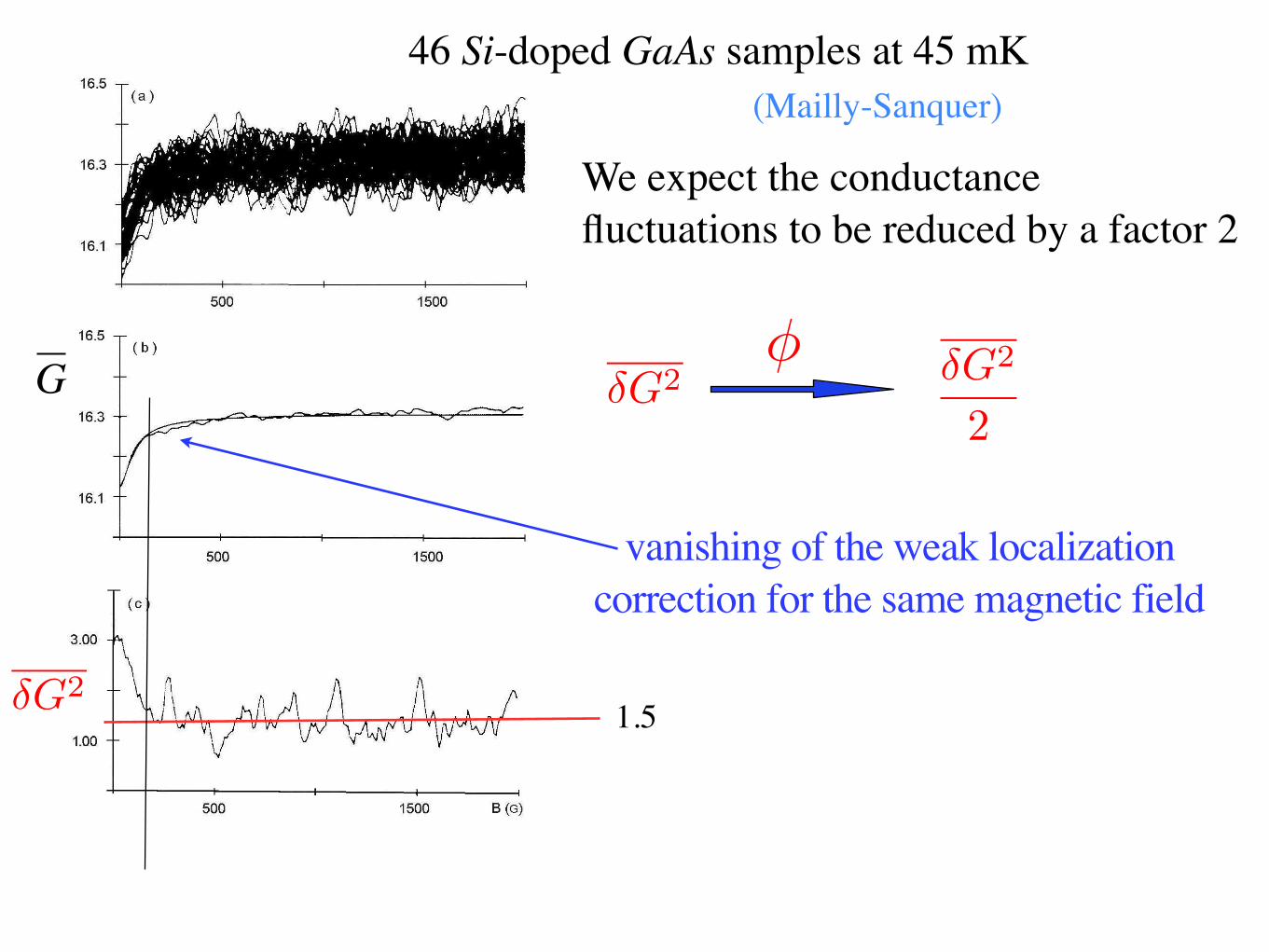
δG2 δG2
2
φ
1.5
vanishing of the weak localization correction for the same magnetic field
In the presence of incoherent processes : L > Lφ
δG2→ 0
46 Si-doped GaAs samples at 45 mK
δG2
�
G
(Mailly-Sanquer)

We expect the conductance fluctuations to be reduced by a factor 2
δG2 δG2
2
φ
1.5
vanishing of the weak localization correction for the same magnetic field
In the presence of incoherent processes : L > Lφ
δG2→ 0
46 Si-doped GaAs samples at 45 mK
δG2
�
G
(Mailly-Sanquer)

We expect the conductance fluctuations to be reduced by a factor 2
δG2 δG2
2
φ
1.5In the presence of incoherent processes : L > Lφ
δG2→ 0
46 Si-doped GaAs samples at 45 mK
δG2
�
G
(Mailly-Sanquer)

We expect the conductance fluctuations to be reduced by a factor 2
δG2 δG2
2
φ
1.5In the presence of incoherent processes : L > Lφ
δG2→ 0
46 Si-doped GaAs samples at 45 mK
δG2
�
G
(Mailly-Sanquer)
We expect the conductance fluctuations to be reduced by a factor 2
δG2 δG2
2
φ
1.5
vanishing of the weak localization correction for the same magnetic field
In the presence of incoherent processes : L > Lφ
δG2→ 0
46 Si-doped GaAs samples at 45 mK
δG2
�
G
(Mailly-Sanquer)

We expect the conductance fluctuations to be reduced by a factor 2
δG2 δG2
2
φ
1.5
vanishing of the weak localization correction for the same magnetic field
In the presence of incoherent processes : L > Lφ
δG2→ 0
46 Si-doped GaAs samples at 45 mK
δG2
�
G
(Mailly-Sanquer)

Thank you for your attention.
Based on Mesoscopic physics of electrons and photons, by Eric Akkermans and Gilles Montambaux, Cambridge University Press, 2007
8/20/17, 2:14 PM51DXRKK5vgL._SX346_BO1,204,203,200_.jpg 348×499 pixels
Page 1 of 1https://images-na.ssl-images-amazon.com/images/I/51DXRKK5vgL._SX346_BO1,204,203,200_.jpg