Mesoscopic Multi-particle Collision Model for Fluid Flow ...rkapral/Papers/meso_rev.pdf · It is well known that the hydrodynamic equations of motion are a macroscopic ... Mesoscopic

Mesoscopic Multi-particle Collision Modelfor Fluid Flow and Molecular Dynamics

Anatoly Malevanets1 and Raymond Kapral2

1 Flow Software Technologies 3070 Jefferson Blvd., Windsor, ON N8T 3G9, Canada2 Chemical Physics Theory Group, Department of Chemistry, University of Toronto, Toronto,

ON M5S 3H6, Canada

Abstract. Several aspects of modeling dynamics at the mesoscale level are discussed: (1) Theconstruction of a mesoscopic description of fluid dynamics. The mesoscale dynamics consists offree streaming interrupted by multi-particle collisions. The multi-particle collisions are carried outby performing random rotations of particle velocities in predetermined cells in a manner that con-serves mass, momentum and energy. The algorithmic implementation of the method is describedand its theoretical basis is justified. Examples of simulation results on hydrodynamic flows arepresented. (2) A hybrid molecular dynamics (MD)-Mesoscale Solvent model is described next.In this method full MD of solute particles is combined with the mesoscale dynamics of the sur-rounding fluid. The method is illustrated by considering the diffusive dynamics and hydrodynamicinteractions among solute particles and clusters in the mesoscale solvent. (3) Finally, extensionsof such schemes are outlined. In particular, generalizations to molecular solvents are presentedand examples of solute dynamics in mesoscale water are given; also extensions to reactive flowsare described.

1 Introduction

It is well known that the hydrodynamic equations of motion are a macroscopic man-ifestation of the microscopic conservation laws of mass, momentum and energy. Thisobservation has prompted the construction of mesoscopic models whose dynamics maybe simplistic in comparison to that of real fluids but which preserve these conserva-tion laws and lead to the hydrodynamic equations on macroscopic distance and timescales. Perhaps the best known models of this class are lattice gas automata and latticeBoltzmann equations. Lattice gas automata for hydrodynamics often suffer from latticeartifacts that have limited their use, but they have proven their utility for the simulationsof complex fluids or fluid flows in complex geometries [1,2]. Lattice Boltzmann meth-ods [3] have been developed extensively and have been used to investigate a variety ofproblems ranging from hydrodynamic flows to fluid flows in complex geometries andcomplex systems [4–6].

In this chapter we discuss a particle-based mesoscopic model for the descriptionof hydrodynamic fluid flow and solute molecular dynamics [7,8]. The fictitious parti-cles of the model are not restricted to the sites of a lattice and thus particle positionsand velocities can take on continuous values. The dynamics consists of free stream-ing interrupted by multi-particle collisions that change the particle velocities. Formally,the multi-particle collision dynamics is constructed as a superposition of propagators

A. Malevanets and R. Kapral, Mesoscopic Multi-particle Collision Model for Fluid Flow and Molecular Dynamics, Lect.Notes Phys. 640, 116–149 (2004)http://www.springerlink.com/ c© Springer-Verlag Berlin Heidelberg 2004

Mesoscopic Multi-particle Collision Dynamics 117

corresponding to these processes which act in position-momentum space and conservemomenta, energy and phase space volume. As a result, one may demonstrate that theexact full set of hydrodynamic equations is obtained in the macroscopic limit. We focusour attention on two specific types of propagator: Free-streaming propagator, arisingfrom integration of the equations of motion for non-interacting molecules, and collisionpropagator, exchanging momenta among particles in a collision cell. The model differsfrom lattice Boltzmann models in that it is not a discrete simulation of a Boltzmannequation for a single particle distribution function, rather, it is a mesoscopic moleculardynamics which possesses the stability properties of particle-based methods. It is akin toDirect Simulation Monte Carlo (DSMC) methods [9] with a more efficient multi-particlecollision dynamics.

The model should prove especially useful for applications to the dynamics of complexfluids and complex systems. Because of its particle nature, a hybrid version of themodel that combines mesoscopic multi-particle collision dynamics with full moleculardynamics of embedded molecules or particles is easily constructed. Detailed featuresof the intermolecular forces between the mesoscopic solvent particles and the solutemolecules are naturally taken into account. This permits potential applications of themodel to large biomolecule or polymer dynamics in solution or to the dynamics ofcolloidal suspensions. For these systems the fluctuations intrinsic in the mesoscopicparticle dynamics are an advantageous feature. Consequently, the model should seeapplications to a number of problems in biophysics and the rheology of complex systems.

The outline of the chapter is as follows: In Sect. 2 we describe the constructionof the model and outline some of its main properties. Section 3 demonstrates how thehydrodynamic equations of motion can be deduced from the dynamics by the applicationof projection operator methods. In this section discrete Green–Kubo expressions forthe transport properties are derived. Some illustrations of the utility of the scheme forsimulations of fluid flow are described in Sect. 4. The hybrid scheme for moleculardynamics in the mesoscopic solvent is formulated in Sect. 5 while applications arediscussed in Sect. 6. The conclusions are given in Sect. 7.

2 Multi-particle Collision Model for Fluid Flow

A simplified version of molecular collision dynamics in a fluid that yields the correcthydrodynamic equations on long distance and time scales can be constructed in thefollowing way. We adopt a mesoscopic view of the fluid which involves discrete timeupdating of continuous particle positions and velocities through both free streaming andcollisions. The dynamics is constructed so that the conservation laws of mass, momentumand energy are satisfied, an essential feature in any dynamical scheme.

Consider a system comprisingN particles, each with massm. 1 The particle positionsand velocities are denoted by X(N) = x1,x2, . . . ,xN andV(N) = v1,v2, . . . ,vN, respectively. The dynamics consists of free streaming,

xi(t+ τ) = xi(t) + vi(t)τ , (1)

1 The mesoscopic collision dynamics is easily generalized to systems where the particles havedifferent masses.

118 A. Malevanets and R. Kapral

Fig. 1. Schematic representation of the division of a system into cells for the application of themulti-particle collision rule. The particle positions are continuous variables and are not confinedto the cell centers. The velocities are also continuous and are denoted by lines in the figure

interspersed by multi-particle collisions at discrete time intervals τ . The post-collisionvelocities after multi-particle collisions [10] are determined by first dividing the systeminto cells as shown schematically in Fig. 1. At each time interval rotation operators ωξ

are chosen at random from a set Ω of rotation operators and assigned to the cells. LetVξ be the center of mass velocity of the particles in cell ξ,

Vξ =1nξ

∑

i|x∈Vv′

i ,

where nξ is the number of particles in the cell with volume V and v′i is the pre-collision

value of the velocity. The post-collision velocity vi of every particle i in cell ξ is givenby

vi = Vξ + ωξ(v′i − Vξ) . (2)

The same rotation operator is applied to every particle in the cell but it differs from cellto cell. This simple collision rule changes both the directions and magnitudes of theparticle velocities in the cell as can be seen from the two-dimensional example for twoparticle velocities shown in Fig. 2. The collision rule conserves mass, momentum andenergy within each cell. This can be seen by summing the post-collision momenta andenergies in each cell. For the momentum and energy we have, respectively,

∑

i|x∈Vmvi =

∑

i|x∈Vm(V + ω[v′

i − V])

=∑

i|x∈Vmv′

i , (3)

∑

i|x∈V

m

2‖vi‖2 =

∑

i|x∈V

m

2

∥∥V + ω[v′

i − V]∥∥2 =

∑

i|x∈V

m

2‖v′

i‖2 . (4)

In addition, one may show that the dynamics preserves phase space volumes [7].As discussed above, in order to apply the multi-particle collision rule the system

must be divided into cells where the collisions occur. The choice of cell size is dictated


V

v1

v2

v2

v1

v1- V

v2- Vv2- V( )

v2- V( ) v1- V )VV− −

ω ω

ω

v1- V )(

ω (

’

’’

’

’

’

’

’

’

’Fig. 2. Multi-particle collision rule applied to two particles in two dimensions for a rotation byπ/2. The dark arrows labelled v′

1 and v′2 denote the pre-collision velocities. The upper panel also

shows the center of mass velocity and the pre-collision velocities relative to the center of massbefore and after rotation by π/2. The lower panel shows the result of adding back the center ofmass velocity to yield the post-collision velocities. Both the velocity directions and magnitudesare changed as a result of the collision

by the particle density and the mean velocity of the particles in the system. The particledensity determines the mean number of particles per cell and thus affects the numberof particles involved in a multi-particle collision event. The mean velocity determines,on average, how far particles travel between collision events. Multi-particle collisionswill be efficient if large numbers of particles participate in each collision event. In orderto avoid correlations between collisions, particles should travel on the order of a celllength between collisions. Consideration of these factors provides rough guides for theappropriate choice of the collision cell size.

Once the system has been partitioned into cells of suitable size, a specific form forthe particle velocity rotation operators must be chosen. This choice will also influencethe magnitudes of the transport properties of the fluid. Consider a three-dimensionalsystem. It is convenient to take rotations about a randomly chosen direction, n, by anangleΦ chosen from a set of angles. For this choice, the contribution to the post-collisionvelocity vi of particle i in cell ξ, vi = Vξ + ωξ(v′

i − Vξ), arising from the rotation isgiven explicitly by

ωξ(v′i − Vξ) = nn · (v′

i − Vξ) + (I− nn) · (v′i − Vξ) cosΦ− n× (v′

i − Vξ) sinΦ.(5)


The unit vector n may be sampled uniformly from the surface of a sphere, while theangles Φ may be chosen in any convenient way. For example, convenient choices are toselect Φ randomly from the set π/2,−π/2, or from the set of all angles 0 ≤ Φ ≤ π.

A more elegant way to implement the collision rule is to represent a rotation matrixas a unit quaternion ωξ, and a velocity vector as a pure quaternion v = (0, vx, vy, vz).For this choice, the contribution to the post-collision velocity vi of particle i in cell ξ,with slight abuse of notation, is written as vi = Vξ + Adωξ

· (v′i − Vξ), where the

conjugation operation is defined as

Adx · y = xyx∗ .

One can verify that the conjugation operation preserves the structure of the rotationgroup SO(3) and transforms the vector space of pure quaternions into itself. A unitquaternion ωξ can be generated by sampling vectors uniformly from unit ball B ∈ R4

and subsequent scaling of the resulting vector.

2.1 Evolution Equation

In order to carry out a detailed analysis of the model, one may write the dynamics ofthe system in terms of an evolution equation for the phase space probability density,P(V(N),X(N), t

), which takes the form,

P(V(N),X(N) + V(N)τ, t+ τ

)= CP(V(N),X(N), t

). (6)

The displaced position on the left hand side reflects the free streaming between collisionswhile the collision operator C on the right hand side is defined by

CP(V(N),X(N), t)

=1‖Ω‖L

∑

ΩL

∫

dV′(N)P(V′(N),X(N), t

)

×N∏

i=1

δ(vi − Vξ − ωξ[v′

i − Vξ]).

Here L is the number of cells and ‖Ω‖L is the number of rotation operators in the set.Introducing the free streaming Liouville operator,

iL0 = V(N) · ∇X(N) , (7)

we may write (6) in the alternative form,

eiL0τP(V(N),X(N), t+ τ

)= CP(V(N),X(N), t

). (8)

Using this expression it is instructive to write the evolution equation in continuous timewith a delta function collision term,

∂

∂tP (X(N),V(N), t) =

(− iL0 + C

)P (X(N),VN), t) , (9)


where the collision operator C acts at discrete time intervals on the velocities of theparticles and is defined as

CP (X(N),V(N), t) =∞∑

m=0

δ(t−mτ)(C − 1)P (X(N),V(N), t) . (10)

The reduction of the evolution equation (9) to the discrete form (8) can be carried outby integrating (9) from t = mτ + ε to t+ τ where ε is an infinitesimal number.

The evolution equation (6) can be written in a more compact form by letting Γ =(V(N),X(N)) denote a phase point and defining a transition operatorW(Γ ′ → Γ ) thataccounts for the streaming and collision steps. The discrete-time evolution equation maythen be written as

P(Γ, t+ τ) =∫

dΓ ′W(Γ ′ → Γ )P(Γ ′, t) ≡ WP(t), (11)

where the integral implies summation over any preimages of the stateΓ . More explicitly,the transition operator has the definition,

∫

dΓ ′W(Γ ′ → Γ )P(Γ ′, t) =1‖Ω‖L

∑

ΩL

∫

dV′(N)dX′(N) ×

×N∏

i=1

δ(vi − Vξ − ωξ[v′

i − Vξ])δ(x′

i − (xi + viτ))P(V′(N),X′(N), t

).

The distribution of this Markov chain is denoted by P0(Γ ) = P0(V(N),X(N)) inequilibrium. Assuming the system is ergodic, in view of the conservation laws obeyedby the dynamics, the stationary distribution is given by the microcanonical ensembleexpression,

P0(Γ ) = N δ(

1N

N∑

i=1

m

2‖vi‖2 − d

2β

)

δ

(N∑

i=1

[vi − u]

)

, (12)

where u is the mean velocity of the system andN is a normalization constant. If (12) isintegrated over the coordinates and velocities of particles with labels i = 2, . . . , N , theMaxwell distribution,

Pm(v1,x1) =1V

(mβ

2π

)d/2

exp(−βm‖v1 − u‖2/2) , (13)

is obtained in the limit of large N . Here β = (kBT )−1, V is the system volume and dis the dimension.

2.2 H-Theorem

While the above arguments indicate that the equilibrium one-particle distribution func-tion is Maxwellian, it is instructive to establish an H-theorem for relaxation to equilibrium


for the multi-particle collision dynamics [7]. In the Boltzmann approximation where thefull phase space probability distribution function P is a product of identical one-particleprobability distributions,

P(V(N),X(N), t) =N∏

i=1

P1(vi,xi, t) , (14)

it is possible to derive such a relation as we now show.Letting f(v,x, t) = NP1(v,x, t), the H-functional is defined in terms of the reduced

one-particle distribution function as,

H(t) =∫

dvdx f(v,x, t) ln f(v,x, t)

=∑

ξ,n∈N

e−ρξ

n!

∫

Vn

dV(n)dX(n)n∏

i=1

f(vi,xi, t) lnn∏

i=1

f(vi,xi, t) , (15)

where the second equality follows from the representation of the system in terms ofphase space cells and makes use of the resolution of identity 1 =

∑

n≥0

e−xxn

n! . ThatH(t)

decreases on each discrete evolution step may be proved using the convexity inequality,

∑

s

A(s)B(s) lnB(s) ≥(∑

s

A(s)B(s))

ln(∑

s

A(s)B(s))

, (16)

where A is normalized so that∑

sA(s) = 1. We define R(n) by

R(n)(V(n),V′(n)) =1‖Ω‖

∑

ω∈Ω

n∏

i=1

δ(vi − V + ω[V − v′

i]), (17)

whose integral over V′(n) is unity. Making use of R(n), we may write (15) in the form

H(t) =∑

ξ,n∈N

e−ρξ

n!

∫

Vn

dV(n)dX(n)n∏

i=1

f(vi,xi, t)

× lnn∏

i=1

f(vi,xi, t)∫

dV′(n)R(n)(Vn,V′(n)) . (18)

Next, we exchange the order of the V′(n) and V(n) integrations in each term in the sumand use (16) to write

∫

dV(n)R(n)(V(n),V′(n))n∏

i=1

f(vi,xi, t) lnn∏

i=1

f(vi,xi, t)

≥ f(n)(V′(n),X(n), t) ln f(n)(V′(n)

,X(n), t) , (19)


where

f(n)(V′(n),X(n), t) =

∫

dVnR(n)(V(n),V′(n))n∏

i=1

f(vi,xi, t) .

As a result of these manipulations we obtain,

H(t) ≥∑

ξ,n∈N

e−ρξ

n!

∫

Vn

dV′(n)dX(n) f(n)(V′(n),X(n), t) ln f(n)(V′(n)

,X(n), t). (20)

To simplify this expression, we let

A =n∏

i=1

f(n)i , B =

f(n)(V′(n),Xn, t)

Z∏n

i=1 f(n)i

,

where Z and f(n) are defined as

Z =∫

Vn

dV′(n)dX(n) f(n)(V′(n),X(n), t) = ρn

ξ , (21)

f(n)i (v′

i,xi, t) =1Z

∫

V[n−1]

dv′1dx1 · · ·dv′

idxi · · ·dv′ndxn f(n)(V′(n)

,X(n), t), (22)

where integrations over variables with a hat in (22) are omitted. Substituting A and Binto (16) we find

1Z

∫

Vn

dV′(n)dXn f(n)(V′(n),X(n), t) ln

f(n)(V′(n),X(n), t)

Z∏n

i=1 f(n)i

≥

∫

Vn

dV′(n)dX(n) f(n)(V′(n),X(n), t)Z

ln∫

Vn

dV′(n)dX(n) f(n)(V′(n),X(n), t)Z

=0 . (23)

Since the argument of the logarithm is unity given the definition of Z, the last term in(23) is equal to zero. From (23) it follows that

∫

Vn

dV′(n)dX(n) f(n)(V′(n),X(n), t) ln f(n)(V′(n)

,X(n), t)

≥∫

Vn

dV′(n)dX(n) f(n)(V′(n),X(n), t) lnZ

n∏

i=1

f(n)i .

Finally, using the identity,

n∑

i=1

∫

Vn

dv′ixiZ f(n)

i (v′i,xi, t) lnZ1/n f(n)

i (v′i,xi, t) =

=∫

Vn

dV′(n)dX(n) f(n)(V′(n),X(n), t) lnZ

n∏

i=1

f(n)i (v′

i,xi, t) ,


in (20) we have,

H(t) ≥∑

i,ξ,n∈N1

e−ρξρn−1ξ

n!

∫

Vdv′dxZ1/n f(n)

i (v′,x, t) lnZ1/n f(n)i (v′,x, t)

≥∫

dv′dxC(f) ln C(f) =∫

dv′dxf(v′,x, t+ 1) ln f(v′,x, t+ 1) .

The second inequality follows from the application of (16) with A given by the Poissondistribution A(n) = (e−ρξρn−1

ξ )/[(n− 1)!], and the last equality follows from theinvariance of the integral with respect to translations by the streaming transformation.Therefore, the value of the H functional at time t+ τ does not exceed its value at timet so that

H(t) ≥∫

dv′dxf(v′,x, t+ τ) ln f(v′,x, t+ τ) . (24)

System Thermalization. In order to confirm these predictions, we study the thermal-ization of a system obeying multi-particle collision dynamics. We consider a three-dimensional system with density ρ = 2 in a box of length L = 40 with periodicboundary conditions which is partitioned into 40×40×40 cells of unit length. The tem-perature in reduced units (m = 1, τ = 1, and unit cell length) is taken to be kBT = 4/3.We study the equilibration of a system initialized by f(v) = 1

2δ(v+v0)+ 12δ(v−v0),

where v0 = (2, 0, 0). The results of such a simulation after relaxation to equilibrium areshown as a histogram of the x-component of the velocity in Fig. 3. One can see that aBoltzmann distribution of velocities is obtained.

It is instructive to examine the relaxation to equilibrium of the multi-particle colli-sion dynamics in more detail. For this purpose, it is convenient to rewrite one-particleprobability distribution as a sum of Hermite polynomials ,

f(vx) = ζ−1e−(vx/ζ)2∑αiHi(vx/ζ), (25)

where ζ =√

2kBT/m. The expansion coefficients are easily obtained from the expec-tation values of Hermite polynomials,

(−1)nn!2n√παn = 〈Hn(vx/ζ)〉. (26)

The expansion coefficients are less sensitive to fluctuations than histograms (Fig. 3) anddemonstrate fast convergence to local equilibrium.

In Fig. 4 we plot the values of the expansion coefficients as a function of time. Usingthe above expansion and assuming the system is spatially homogeneous, we may writefor velocity component of the one-particle probability distribution

−Hv =∫

dvf(v) ln f(v) = 〈ln f(v)〉. (27)

Approximating f(v) by the Hermite polynomial expansion to obtain the results, weplot values of theH-function in a non-equilibrium run. As expected from the theoreticalanalysis, the functional increases monotonously with time and rapidly converges to theequilibrium value.


-6.0 -4.0 -2.0 0.0 2.0 4.0 6.0vx

0

0.1

0.2

0.3

0.4

P(v

x)

Fig. 3. Histogram of the velocity distribution in the system at equilibrium. The system hasN = 5.1 × 106 particles, kBT = 4/3 and ρ = 2.0. The solid line is the calculated distribu-tion based on an expansion of the distribution function using ten Hermite polynomials (see text)

0 2 4 6 8 10Steps, t

-0.10

-0.08

-0.06

-0.04

-0.02

0.00

0.02

an

Fig. 4. Dynamics of the coefficients of the Hermite polynomials of a system relaxing to equi-librium. Coefficients of H2(vx)-(solid line), H4(vx)-(dotted line) and H6(vx)-(dotted line) areplotted. Odd coefficients vanish due to symmetry and the coefficient of H0 is equal to one bydefinition


0 5 10 15 20Steps, t

-1.6

-1.5

-1.4

-1.3

-1.2

-Hv(t

)

Fig. 5. Evolution of the velocity component of the H-function from non-equilibrium initial con-ditions. Details are given in the text

3 Hydrodynamic Equations and Transport Properties

The dynamics described above is very simple, both in its conception and in its implemen-tation. However, it is essential to provide a theoretical underpinning for the mesoscaledynamics to be able to assess its properties and to demonstrate that it yields the correcthydrodynamic equations. In this section we use projection operator methods to reducethe multi-particle collision dynamics to hydrodynamic equations for the conserved fields.As a by-product of this derivation we also obtain correlation function expressions forthe transport properties of the system that can be used for their calculation.

3.1 Evolution Equations for Mean Dynamical Variables

The projection operator methods we use are based on methods developed for continuous-time deterministic systems [11,12]. Modifications of the projection operator techniquesmust be made to account for the intrinsic stochasticity and discrete-time dynamics of themesoscopic dynamics [13]. We first present the derivation of a general set of projectedequations and then specialize the projection operator to one that depends on the conservedfields.

In order to derive a set of evolution equations for the mean values of a set of dynamicalvariables a, we introduce a projection operator P by,

(Ph)(Γ ) = a†(Γ )P0(Γ )⟨aa†⟩−1

∫

dΓ ′a(Γ ′)h(Γ ′),


where h(Γ ) is any function of the phase space variables. The dagger denotes the adjointand the angular brackets symbolize an average over the equilibrium distribution, i.e.,

〈· · · 〉 =∫

dΓ · · ·P0(Γ ) .

The complementary operator Q is defined by Q = 1 − P . Applying the projectionoperators P and Q to (11) we obtain a system of two equations,

PP(t+ τ) = PWPP(t) + P(W − 1)PQ(t), (28)

PQ(t+ τ) = Q(W − 1)PP(t) +QWPQ(t), (29)

where PP(t) = PP(t) and PQ(t) = QP(t). To facilitate some of the calculationspresented below, we have replaced W by W −1 in certain terms where this replacementhas no effect because PQ = 0. Solving (29) by iteration leads to

PQ(t) =[QW]t

PQ(0) +n∑

=1

[QW]−1Q(W − 1)PP(t− τ) , (30)

where t = nτ . Substitution of this result into (28) gives

PP(t+ τ) = PWPP(t) +n∑

=1

K(− 1)PP(t− τ), (31)

where the memory kernel is defined by

K() = P(W − 1)[QW]Q(W − 1

)P. (32)

The first term on right hand side of (30) was eliminated by the use of a specially preparedensemble of initial conditions where deviations from equilibrium occur only in thedynamical variables in the set a so that PQ(0) = 0.

From (31) we can easily derive a set of equations for the average values of thedynamical variables,

a(t) =∫

dΓa(Γ )P(Γ, t) , (33)

by multiplying this equation from the left by a and integrating over the phase spacevariables to obtain,

a(t+ τ) − a(t) =⟨a(W − 1

)a†

⟩ ⟨aa†⟩−1

a(t) +t∑

=1

K(− 1)a(t− τ) , (34)

where

K() =⟨a(W − 1

)[QW]Q(W − 1

)a†

⟩ ⟨aa†⟩−1

.


For slowly decaying dynamical variables, which are our main concern, a(t − τ) canbe replaced by a(t) and the upper limit on the sum can be replaced by infinity. In thisapproximation (34) becomes the kinetic equation

a(t+ τ)− a(t) =(Ω + Φ

)a(t) , (35)

where the matrices Ω and Φ are given by

Ω =⟨a(W − 1

)a†

⟩ ⟨aa†⟩−1

, (36)

Φ =∞∑

=1

K(− 1) .

We now analyze the structure of (35) for the specific choice of conserved dynamicalvariables.

3.2 Kinetic Equations for Conserved Variables

The hydrodynamic equations describe the dynamics of the conserved mass, momentumand energy density fields. The microscopic fields corresponding to these variables, whichare relevant for the multi-particle collision dynamics, are the particle density along withmomentum (or, equivalently, velocity for equal mass particles) and energy densities ina cell,

ρ(x) =N∑

i=1

δ(xi − x) , (37)

µ(ξ) =N∑

i=1

viθ(1/2− |xi − ξ|) , (38)

ε(ξ) =N∑

i=1

m

2v2i θ(1/2− |xi − ξ|) .

Here θ is the Heaviside function. Since the hydrodynamic equations are valid on distanceand time scales which are long compared to molecular scales, it is convenient to workwith the Fourier transforms of these fields and then consider the small k limit. TheFourier transforms of these variables are given by,

ρk =∫

dx eik·xρ(x) =N∑

i=1

eik·xi , (39)

µk =∑

ξ

eik·ξµ(ξ) =N∑

i=1

vi

∑

ξ

eik·ξθ(1/2− |xi − ξ|) , (40)

εk =∑

ξ

eik·ξε(ξ) =N∑

i=1

m

2v2i

∑

ξ

eik·ξθ(1/2− |xi − ξ|) .


Rather than dealing with this set of variables directly, it is useful to define an orthogonalset of dynamical variables, ak = ρk,µk, sk, where the entropy density is defined assk = εk −CvTρk with Cv the specific heat. In terms of this set of variables the matrix⟨aka

†k

⟩is diagonal and given by

⟨aka

†k

⟩= N

1 0 00 (kBT/m)1 00 0 CvkBT

2

, (41)

where Cv = 3kB/2 in three dimensions. Using this statistically independent set ofvariables simplifies the algebraic manipulations. When confusion is unlikely to arise,we shall simplify the notation and drop the subscripts k on the vectors of dynamicalvariables. In view of the fact that one is primarily interested in the evolution of theconserved variable fields, we specialize the general kinetic equation (35) to this caseand, in particular, we determine the forms of the Ω and Φ matrices.

Structure of the Ω Matrix. We first construct the form of the matrix Ω to O(k2) forconserved fields. For this purpose it is convenient to introduce an operator S(Γ, t) whichrelates the state Γ at the initial time to the set of states at time t, weighted with theprobability of transition to the corresponding state. In terms of this notation, equilibriumaverages may be written as

∫

dΓ∫

dΓ ′a(Γ )W(Γ ′ → Γ )h†(Γ ′)P0(Γ ′) =⟨a(S(Γ, τ))h†(Γ )

⟩,

where summation over states is implied. Similarly, if we consider the equilibrium averageof a set of dynamical variables, using the stationarity of the equilibrium distribution,P0(Γ ) = WP0(Γ ), we may write,

∫

dΓh†(Γ )P0(Γ ) =∫

dΓh†(Γ )WP0(Γ ) =∫

dΓh†(Γ )∫

dΓ ′W(Γ ′ → Γ )P0(Γ ′)

=∫

dΓ ′[ ∫

dΓh†(Γ )W(Γ ′ → Γ )]P0(Γ ′),

≡∫

dΓ ′h†(S(Γ ′, τ))P0(Γ ′) .

From this result we may establish that

⟨a(S(Γ, τ))a†(S(Γ, τ))

⟩=

⟨a(Γ )a†(Γ )

⟩.

Letting b(Γ ) = a(S(Γ, τ))− a(Γ ) we may write Ω as

Ω =⟨ba†⟩ ⟨aa†⟩−1

.


The elements of the b variable vector are given by

bρk = ik ·N∑

i=1

τvi + o(k), (42)

bµk = ik ·N∑

i=1

∆ξivi + o(k), (43)

bεk = ik ·N∑

i=1

∆ξi

m

2v2i + o(k),

where we introduced notation ∆ξi(t) = ξi(t+ τ)− ξi(t) with ξi(t) the coordinate ofthe cell in which particle i is located at time t. One can see that these elements areO(k).

It is useful to rewrite the numerator of Ω as a sum of symmetric and antisymmetricterms; thus, we have

Ω = A− 12⟨bb†⟩ ⟨aa†⟩−1

, (44)

where we defined A as

A =12⟨a(S(Γ, τ))a†(Γ )− a(Γ )a†(S(Γ, τ))

⟩ ⟨aa†⟩−1

.

Using the explicit forms of the conserved mass, momentum and energy density fields,A may be computed to give,

A = NτkBT

m

0 ik 0

ikT 0 ikT kBT0 ikkBT 0

⟨aa†⟩−1

. (45)

In order to write⟨bb†⟩ in the second term of (44) in an alternative form, we introduce

a projection operator onto a dynamical variable as

Ph =⟨ha†⟩ ⟨aa†⟩−1

a. (46)

In terms of this new projection operator we have

12⟨bb†⟩ =

12⟨bQb†⟩ +

12⟨bPb†⟩ =

12⟨f(0)f†(0)

⟩+

12⟨bPb†⟩ , (47)

where we have defined the random forces,

f(0) = b− ⟨ba†⟩ ⟨aa†⟩−1

a = a(S(Γ, τ))− ⟨a(S(Γ, τ))a†⟩ ⟨aa†⟩−1

a. (48)

The explicit expressions for the random forces corresponding to the conserved variablefields are, to lowest order in k,

fρk(t) = 0 + o(k), (49)

fµk (t) = τ

∑

i

(

vi(t)[ik · ∆ξi(t)

τ

]− 1dikvi(t)2

)

+ o(k), (50)

fεk(t) = τ ik ·

∑

i

[∆ξi(t)τ

(m

2vi(t)2 − CvT

)− vi(t)(Cp − Cv)T]

+ o(k).


The term⟨bPb†⟩ ⟨aa†⟩−1

may be expressed as

⟨bPb†⟩ ⟨aa†⟩−1

=⟨ba†⟩ ⟨aa†⟩−1 ⟨

ab†⟩ ⟨aa†⟩−1.

From (44) we have,⟨ba†⟩ ⟨aa†⟩−1

= A + o(k) ,⟨ab†⟩ ⟨aa†⟩−1

= −A + o(k).

Consequently, it follows that⟨bPb†⟩ ⟨aa†⟩−1

= −A2 + o(k2).

Assembling all of these results, the net effect of these manipulations is that the Ωmatrix may be written as

Ω = A +12A2 − 1

2⟨f(0)f†(0)

⟩ ⟨aa†⟩−1

+ o(k2).

Structure of the Φ Matrix. In order to write the Φ matrix in a convenient form, we firstshow that the projected dynamics can be replaced by ordinary dynamics in the small klimit for conserved variables. If the dynamics is given by a composition of streamingand collision operators in that order, we may write,

ak =∑

i

ai(t)eik·xi(t) =∑

i

ai(t− τ)eik·xi(t), (51)

where ai is a conserved variable. This result follows from the conservation of the quan-tities a under collisions at time t− τ . Using the identity (51) and expanding a in powersof k, we may write P[W − 1

]h†, where h† is an arbitrary function, as

(P[W − 1]h†)(Γ ) = a†P0(Γ )

⟨aa†⟩−1

∫

dΓ ′b(Γ ′)h†(Γ ′)

= a†P0(Γ )⟨aa†⟩−1

∫ ∫

Γ ′[

h†(Γ ′)

∑

i

(ik · [x′

i(t+ τ)− x′i(t)

]a′

i(t) + o(k))]

. (52)

Similarly, one may show that[W − 1

]P = O(k).Using these results we may prove by induction that

[QW]Q = QWtQ+O(k). (53)

For = 0 relation (53) holds; we assume that it holds for and prove the relation for

+ 1. We write[QW]+1Q =

[QW]QWQ. Then

[QW]+1Q =[QW]QWQ = QWQWQ+O(k)

= QW[Q+

(W − 1)

+O(k)]Q+O(k)

= QW+1Q+O(k),


where we expressed QW in the equivalent form

QW = Q+(W − 1

)− P(W − 1)

= Q+(W − 1

)+O(k). (54)

This proves the assertion of the recursion relation and, thus, the validity of (53).The correlation function in the definition of the Φ matrix can now be written as

K(− 1)⟨aa†⟩ =

⟨a(W − 1

)QW−1Q(W − 1)a†

⟩=

⟨f()f(0)

⟩, (55)

with

f() = a(S(Γ, (+ 1)τ))− ⟨a(S(Γ, τ))a†⟩ ⟨aa†⟩−1

a(S(Γ, τ)) , (56)

and

f(0) = a† − a†(S(Γ, τ))⟨aa†⟩−1 ⟨

a(S(Γ, τ))a†⟩ .

The last step in the analysis of Φ is to rewrite the expression for f(0) for conservedvariables fields for small k. We may write,

f†(0) + f(0) = −b† ⟨aa†⟩−1 A ⟨aa†⟩ +

12(a† + a†(S(Γ, τ))

) ⟨aa†⟩−1 ⟨

bb†⟩

= O(k2) .

Making use of this result, the Φ matrix to order O(k2) takes the form,

Φ = −∞∑

=1

⟨f()f†(0)

⟩ ⟨aa†⟩−1

.

3.3 General Form of the Kinetic Equation

In order to use these results to write the kinetic equations in the form of the hydrodynamicequations, we consider the passage from discrete-time to continuous-time dynamics.From the analysis presented above, the sum of the Ω and Φ matrices may be written interms of contributions of O(k) and O(k2), respectively, as

Ω + Φ = A−B ,where

B = −12A2 +

12⟨f(0)f†(0)

⟩ ⟨aa†⟩−1 −Φ .

The matrices A and B are of the first and second orders in k, respectively. The evolutionequation (35) can be written as

a(t+ τ) = eτ ∂∂t a(t) =

(1 + A−B)

a(t) ,

so that we have the operator identity

eτ ∂∂t = 1 + A−B .


Taking the logarithm of this operator identity and expanding the logarithm in a Taylorseries up to second order in k we obtain

τ∂

∂t= A− 1

2A2 −B,

= A− 12⟨f(0)f†(0)

⟩ ⟨aa†⟩−1 −

∞∑

=1

⟨f()f†(0)

⟩ ⟨aa†⟩−1

. (57)

Using this relation, the continuous-time limit of (35) is given by

τ∂ta = Aa−

limT→∞

12T

∑

,′′<T

⟨f()f†(′)

⟩ ⟨aa†⟩−1

a .

(58)

The second term on the right hand side provides expressions for the transport coefficientsin terms of discrete-time sums of autocorrelation functions. In writing this equation weused the notation,

limT→∞

12T

∑

,′<T

⟨f()f†(′)

⟩=

12⟨f(0)f†(0)

⟩+

∞∑

=1

⟨f()f†(0)

⟩. (59)

3.4 Hydrodynamic Equations

All that remains in the derivation is to substitute the explicit forms of the conservedfields to obtain the hydrodynamic equations. To separate the shear and bulk viscositycontributions one may write the momentum random force as a sum terms which areparallel and perpendicular to k,

fµk (t) = τ

∑

i

(

v⊥i (t)ik · ∆ξ⊥

i(t)τ

+ ik[v‖

i (t)∆ξ‖

i(t)τ

− 1dvi(t)2

])

+ o(k),

where v‖i and v⊥

i are the parallel and perpendicular components of the velocity, respec-tively. Then, using this decomposition of the random force and the explicit expressionfor the A matrix, we find that the linearized hydrodynamic equations take the form,

∂tρk = ik · µk, (60)

∂tµk = ik · [kBTρk +skcv

]− η

mρ

[kk− 1

dk21

]: µk −

ηbmρ

kk : µk (61)

∂tsk = kBT ik · µk −λ

mρk2sk .

The viscosity coefficient is obtained from the auto-correlation of the transverse compo-nent of fµk (t):

η = limT→∞

m2ρ

2kBTNTτ

∑

,′<T

∑

i,j

vxi(τ)∆ξyi(τ)vxj(′τ)∆ξyj(′τ) . (62)


0 2 4 6 8 10τ

0.00

0.02

0.04

0.06

0.08

0.10C

s(τ)

, k B

Tν(

τ)

Fig. 6. Shear viscosity and stress autocorrelation function as a function of time. The circles on thesolid line show computed values of the stress autocorrelation function. The filled diamonds on thedotted line are the results of the partial summation of the autocorrelation function. The parametervalues are ρ = 10.0 and kBT = 1/3

Similarly, the bulk viscosity ηb and heat conductivity λ transport coefficients are givenby the correlation function expressions,

ηb = limT→∞

τmρ

2kBTNT

∑

,′<T

∑

i,j

[

v‖i (τ)

∆ξ‖i(τ)τ

− 1dvi(τ)2

]

×[

v‖j (′τ)

∆ξ‖j(′τ)τ

− 1dvj(′τ)2

]

, (63)

λ = limT→∞

mρ

4CvkBT 2NTτ

∑

,′<T

fεk(τ)fε

k(′τ) . (64)

This rather detailed calculation has served to establish that the mesoscopic multi-particle collision model does lead to the correct full set of hydrodynamic equations onlong distance and time scales. Furthermore, we have derived expressions for the transportproperties of the fluid in terms of discrete-time autocorrelation function expressions thatcan serve as the starting points for computing these properties from simulations of thedynamics.

As an illustration of the calculation of a transport property using the discrete Green-Kubo expression, in Fig. 6 we present the results of numerical simulations of the stress-stress autocorrelation function and shear viscosity. A scattering rule was used where thevelocity was rotated by π/2 in random directions. The simulations were carried out ona three-dimensional system of size 32 × 32 × 32 lattice cells. The figure shows boththe stress-stress autocorrelation function and its time integral, whose asymptotic value


is the solvent viscosity. We note that the stress autocorrelation decays to zero in abouttwo discrete time units, setting the time scale for solvent relaxation.

4 Simulations of Fluid Flow

While the demonstration of the properties of the mesoscopic multi-particle collisionmodel and the derivation of the hydrodynamic equations are rather involved, the dynam-ics may be simulated in a simple and efficient manner. Below we give some examplesof the simulations of fluid flow in order to demonstrate the utility of the model forinvestigations of hydrodynamic flows.

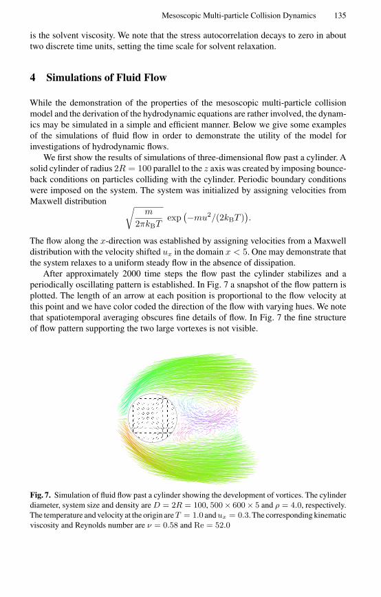
We first show the results of simulations of three-dimensional flow past a cylinder. Asolid cylinder of radius 2R = 100 parallel to the z axis was created by imposing bounce-back conditions on particles colliding with the cylinder. Periodic boundary conditionswere imposed on the system. The system was initialized by assigning velocities fromMaxwell distribution √

m

2πkBTexp

(−mu2/(2kBT )).

The flow along the x-direction was established by assigning velocities from a Maxwelldistribution with the velocity shifted ux in the domain x < 5. One may demonstrate thatthe system relaxes to a uniform steady flow in the absence of dissipation.

After approximately 2000 time steps the flow past the cylinder stabilizes and aperiodically oscillating pattern is established. In Fig. 7 a snapshot of the flow pattern isplotted. The length of an arrow at each position is proportional to the flow velocity atthis point and we have color coded the direction of the flow with varying hues. We notethat spatiotemporal averaging obscures fine details of flow. In Fig. 7 the fine structureof flow pattern supporting the two large vortexes is not visible.

Fig. 7. Simulation of fluid flow past a cylinder showing the development of vortices. The cylinderdiameter, system size and density are D = 2R = 100, 500 × 600 × 5 and ρ = 4.0, respectively.The temperature and velocity at the origin are T = 1.0 and ux = 0.3. The corresponding kinematicviscosity and Reynolds number are ν = 0.58 and Re = 52.0


Fig. 8. Development of the boundary layer at the rear of a disc suddenly set in motion

As another illustration of the method, in Fig. 8 we show the results of simulationsof stages in the development of the boundary layer at the rear of a disk suddenly set inmotion. The system size is 400×400 cells of unit length and the disc diameter 2R = 100.The flow velocity at x = 0, the density of the system and the Reynolds number areux = 0.4, ρ = 20.0 and Re = 1520, respectively. Periodic boundary conditions areimposed on the system and bounce-back conditions on the disc. The initially symmetricflow separates from the disk and a backflow at the far end of the disk develops. At thecontact line between the normal flow and the oppositely-directed backflow, a system ofvortices appears which later expands into the full-scale boundary layer [14].

A series of more detailed studies of the properties of hydrodynamic flows and fluidflow around obstacles of different shapes using the mesoscopic multi-particle collisionmodel were carried out by Ihle and Kroll [15] and Lamura et al. [16,17]. These studiesprovide further evidence of the utility of the method for the investigation of problems inhydrodynamics.

5 Mesoscopic Model for Solute Molecular Dynamics

In this section we show how one may study the dynamics of molecules and other typesof molecular aggregates or particles embedded in a mesoscopic solvent. There are manycircumstances when such an approximate treatment of solvent dynamics is appropriateor necessary. This is the case if one’s primary interest is in the properties of the solutemolecules; then the details of the solvent molecule motions need not be analyzed exceptin so far as they influence solute molecule dynamics. This view of solvent dynamicsunderlies all Langevin and generalized Langevin approximations to condensed phasesystems where the solvent is not explicitly included in the description of the system.Rather than adopting such a extreme reduction of description, we show how one mayconstruct a hybrid molecular dynamics-mesoscopic solvent scheme that eliminates theneed for some of the restrictive assumptions in more phenomenological models.

The system we now consider comprises N solvent or bath molecules (labelled b)with phase space coordinates(V(N),X(N)) introduced earlier, which will be describedat the mesoscopic level, and M solute molecules (labelled s) with phase space coor-dinates X(M) =(xN+1,xN+2, . . . ,xN+M ) and V(M) = (vN+1,vN+2, . . . , vN+M ),which will be described microscopically. The system is demonstrated schematically inFig. 9. We assume the solute molecules interact through the intermolecular potentialVss(X(M)), while the solute-solvent interactions are governed by the potential energyVsb(X(M),X(N)). Since the solvent will be treated at the mesoscopic level using multi-particle collision dynamics, solvent-solvent interactions are set to zero.


M solute molecules N solvent molecules

Fig. 9. Schematic representation of a system following hybrid mesoscopic-molecular dynamics.The small particles are treated at the mesoscopic level while the large particles are treated by fullmolecular dynamics that includes solute-solute and solute-solvent interactions

If we let (X(K),V(K)) = (X(N),X(M),V(N)V(M)) for theK = N+M particles,we can define the classical evolution operator for streaming in the potential energyfunction, V (X) = Vss(X(M)) + Vsb(X) as

iL = V(K) · ∇X(K) + F ·M−1 · ∇V(K) ,

where F = −∇X(K)V (X(K)) is the force and M is a diagonal matrix of masses. Theequation for the evolution of the N + M particle phase space density in the hybridmolecular-mesoscopic dynamics is easily written using this classical evolution operatorand the collision operator C introduced earlier. We have

∂

∂tP(X(K),V(K), t) =

(− iL+ C

)P(X(K),VK), t) ,

where the collision operator C was defined in (10). If we integrate this equation fromt0 = mτ + ε = t to t+ τ we obtain

eiLτP(X(K),V(K), t+ τ) = CP(X(K),V(K), t) . (65)

If the solute molecules are not present, the potential contribution to the evolution operatoriL is zero, and the evolution operator describes free streaming. In this limit (65) reducesto (6).

To implement the dynamics described by (65), we imagine that the phase spacetrajectory of the entire system is partitioned into time segments of length τ within whichone evolves the system by Newton’s equations of motion,

xi = vi

mivi = − ∂V∂xi

= Fi ,

wheremi is the mass of particle i. Such a partitioned phase space trajectory is depictedschematically in Fig. 10. During this Newtonian portion of the evolution the solvent-solvent intermolecular potential is zero; thus, solvent molecules undergo free streamingin the solute-solvent intermolecular potential (assuming they are within range of this


t 0 1t =t0 + τ

∆ tMD segment

collisionsmulti-particle solvent

Fig. 10. Schematic representation of a system trajectory showing the division into MD and seg-ments separated by multi-particle solvent molecule collisions

potential) but do not interact with each other. At discrete time intervals τ the solventmolecules are assumed to undergo multi-particle collisions as discussed in Sect. 2 whichchange the velocities of the solvent molecules. These multi-particle collisions replacethe full solvent-solvent interactions. Since there are no solvent-solvent interactions thismolecular dynamics evolution may be carried out efficiently since it scales with M ×(N+M) rather than (M+N)2. Since typicallyN M this will lead to short simulationtimes compared to full molecular dynamics.

6 Simulations of Hybrid Dynamics

In this section we give some simple illustrations of the implementation of the hybridmesoscopic-molecular dynamics algorithm. In order to carry out such simulations, onemust select a values for the molecular dynamics and multi-particle collision time steps,∆t and τ , respectively. During the molecular dynamics segments∆t for the integrationof Newton’s equations of motion must be chosen to resolve motion in all the forces,including solvent-solute forces. In addition, since the multi-particle collision rule pro-duces momentum jumps in the solvent momenta, an integration scheme must be selectedthat involves the velocities of the molecules, such as the velocity Verlet or leap-frog al-gorithms [18]. The time τ for multi-particle collisions is dictated by several factors.From the perspective of the solvent molecules, τ must be sufficiently large that solventmolecules stream on the order of a cell length in order to ensure sufficient dynami-cal changes in multi-particle collisions. Furthermore, τ should be sufficiently small toincorporate correctly the effect of solvent dynamics on the solute molecules. In suchapplications, typically we are interested in both microscopic (mesoscopic) and collec-tive effects on the solute dynamics. We now show how this hybrid model can be used tostudy some familiar problems in condensed matter physics.

6.1 Brownian Motion

The classical theory of Brownian motion is perhaps one of the best known models ofsolute motion in a solvent whose dynamics is treated approximately [19]. In this theorythe Langevin equation for a Brownian particle takes the form [20,21]

Mdu(t)

dt= −ζu(t) + f(t) , (66)


where r and u are the position and velocity of the Brownian particle with massM , ζ isthe friction coefficient and f is a random force which is usually taken to be a Gaussianrandom process with white noise spectrum,

〈f(t)〉 = 0 and 〈f(t)f(t′)〉 = 2kBTζδ(t− t′) .In this mesoscopic description all information about solute-solvent interactions is con-tained in the friction coefficient which must be evaluated by other means; it is a parameterin phenomenological Brownian motion theory. In general, the friction coefficient con-tains both microscopic and macroscopic (hydrodynamic) contributions whose relativemagnitudes depend on the relative sizes of the Brownian and solvent molecules. Thus,the Langevin approach is not complete unless the friction coefficient and stochastic prop-erties of the random force are determined from the molecular dynamics of the solute andsolvent molecules.

In order to study Brownian motion in the mesoscopic solvent, we consider the dif-fusion of solute particles that interact with the mesoscopic solvent molecules throughcontinuous intermolecular forces. The Hamiltonian that governs the molecular dynamicssegments is

H =12Mu2 +

N∑

i=1

12mv2

i +N∑

i=1

Vsb(|xi − r|) . (67)

For the simulation results presented below, the Brownian particle-solvent interactions,Vsb, are given by truncated LJ potentials,

Vsb(r) =

4ε[σ12

r12− σ

6

r6+

14

]

, r < 21/6σ

0, r > 21/6σ, (68)

with σ = 3.0 and ε = 1.0. In the Newtonian trajectory segments the equations of motionwere integrated using the velocity Verlet algorithm [18] with a time step of∆t = 0.02τ ,which is sufficient to resolve the intermolecular forces. The mass of the Brownian particlewas taken to beM = 250 while the solvent particle mass wasm = 1. The solvent densitywas ρ = 10 and reduced temperature was kBT = 1/3. For these conditions, both themass density ratio, m/M = 0.004 and the mass density ratio, mρ/(M/VB) = 0.45,where the volume of the Brownian particle is VB = 4πσ3/3, are small so that oneexpects simple dynamics [22]. The multi-particle collision dynamics was carried outusing random rotations by ±π/2 about randomly chosen axes as discussed earlier.

The velocity autocorrelation function of the Brownian particle is defined as

Cu(t) =13〈u(t) · u〉 .

The phenomenological theory of Brownian motion based on the Langevin equation (66)predicts exponential decay, Cu(t) = (kBT/M) exp−ζt/M , for all times. For systemswith continuous forces, the Cu(t) must have an initial slope of zero and behave as

Cu(t) ∼ kBTM− 〈F

2〉3M2

t2

2,


for short times. Simulation results using the hybrid mesoscopic model confirm this shorttime behavior. It is more interesting to study the long time behavior of the velocitycorrelation function. While a simple Langevin model predicts exponential decay for alltimes, it is known from both full molecular dynamics simulations [23], kinetic theory[24] and mode coupling theories [25] that the Cu(t) ∼ t−3/2 for long times in threedimensions. The long time tail arises from the coupling between the Brownian particledensity field and the viscous modes of the solvent. Such an effect can also be capturedin a generalized Langevin model,

Mdu(t)

dt= −

∫ t

0dt′ζ(t− t′)u(t′) + f(t) , (69)

where the time dependent friction is evaluated using hydrodynamics [26]. In particular,using the expression for the friction coefficient for a macroscopic particle oscillatingwith frequency ω in an incompressible continuum fluid, [27]

ζ(ω) = ζh

[(1 + ασ)

(1 + ασ/3)+

16(ασ)2

]

, (70)

where the hydrodynamic friction coefficient is ζh = 4πησ for slip boundary conditionsappropriate for our central our system with central forces. The Brownian particle radiushas been set equal to the Lennard-Jones σ parameter for Brownian particle-solventparticle interactions. Here α2 = −iωρM/η. The time-dependent diffusion coefficientD(t) is defined by the finite time integral of the velocity correlation function,

D(t) =∫ t

0dt′Cu(t′) .

Using (69) with (70), the long time behavior of D(t) is given by

D(t) ≈ D − α1√t, where α1 =

23(4πη)−3/2

√Mρ .

This result is valid for either slip or stick boundary conditions. The coefficient of t−1/2

depends only on the Brownian particle mass and the solvent density and viscosity.Figure 11 plots the hybrid mesoscopic model simulation results for D(t) versus t−1/2.One can see from this figure that D(t) does indeed possess a t−1/2 long time tail.Furthermore, the coefficient of this long time decay is in agreement with the predictionsof hydrodynamics: The predicted hydrodynamic value using the mesoscopic solventviscosity is α1 = 0.0114 while the simulation value is approximately 0.0104. Theseresults show that the mesoscopic multi-particle collision dynamics correctly capturesthe collective hydrodynamic component of the Brownian particle diffusion coefficient.

It is also of interest to compare the magnitude of the diffusion coefficient obtainedfrom the simulation with that predicted by simple theories that account for both micro-scopic and hydrodynamic contributions to this transport coefficient. One can view theenvironment of the Brownian particle as being composed of two parts: A boundary layerof microscopic dimensions where details of the intermolecular forces and collision dy-namics are essential and an outer region where a continuum hydrodynamic description


0 0.2 0.4 0.6 0.81/sqrt(t)

0

0.001

0.002

0.003

0.004

0.005

D(t

)

Fig. 11. Long time behavior of the time dependent diffusion coefficient

continuum

region

microscopicboundary

layer

Fig. 12. Boundary layer around a microscopic particle

of the solvent is appropriate. (See Fig. 12 for a schematic picture of this decomposition ofthe environment.) Using a generalized boundary condition in conjunction with a kinetictheory description of the boundary layer one may derive an approximate expression forthe diffusion coefficient of the form, [28]

D = D0 +Dh , (71)

where D0 is a microscopic contribution arising from binary collision events whoseapproximate from can be estimated from kinetic theory,

D0 =3

8ρσ2

(kBT

2πM

)1/2

,

and a hydrodynamic contributionDh = kBT/ζh. The estimates of these quantities are:D0 = 1.0 × 10−3 and Dh = 4.5 × 10−3 giving D = 5.5 × 10−3. The hydrodynamiccomponent dominates the microscopic component for a large Brownian particle. Thevalue of the diffusion coefficient determined from an extrapolation of the simulationdata is D = 4.9× 10−3 which is close to that from the approximate theory.


From these results we conclude that the hybrid mesoscopic dynamics is able captureimportant microscopic and hydrodynamic contributions to the velocity correlation func-tion and diffusion coefficient. It provides a description of the dynamics that goes beyondthat of simple or even generalized Langevin models with approximate expressions forthe time dependent friction.

6.2 Cluster Dynamics

As a somewhat more complicated example we study the dynamics and equilibriumstructure of an aggregate or cluster of microscopic particles in the mesoscopic solvent.Clusters are interesting systems that have been studied extensively both experimentallyand theoretically [29,30]. They have attracted attention since clusters with nanoscaledimensions lie in a regime which is intermediate between the microscopic and macro-scopic domains and exhibit unusual properties as a result of the strong competitionbetween bulk and surface forces. Clusters of Lennard–Jones (LJ) particles with parame-ters that model argon atoms have been studied in vacuum using full molecular dynamics[31–33]. Studies of the properties of such LJ clusters in the mesoscopic solvent provideinformation on how such clusters are influenced by a thermalizing environment [34].

More specifically, we consider a system comprising a cluster whose particles havemassms and interact through attractive LJ forces,

Vss = 4εss

[σ12

ss

r12− σ

6ss

r6

]

,

embedded in the mesoscopic solvent whose particles have massm. The system Hamil-tonian is

H =K∑

i=N+1

12msu2

i +K∑

i<i′=N+1

Vss(|ri − ri′ |) +K∑

i=N+1

N∑

j=1

Vsb(|ri − xj |) +N∑

j=1

12mv2

j

≡ Hs + Vsb +Hb , (72)

whereHs is the cluster Hamiltonian,Hb is the bath Hamiltonian which only has a kineticenergy contribution since solvent-solvent forces are zero, and Vsb is again the clusterparticle-solvent interaction potential which is taken to be a truncated LJ potential (68).The cluster particle interaction parameters are are taken to mimic argon: σss = 0.34 nmand εss = 1.00604 kJ / mol and the values for the cluster particle-solvent moleculeinteractions are εsb = 1.00604 with σsb taking either of two values, σsb = 0.17 nm orσsb = 0.221 nm. The masses of the cluster particles are ms = 39.948 g / mol and thesolvent molecules have massesm = 3.9948 g / mol.

The cubic simulation box had lengthL = 5.44 nm with periodic boundary conditionsand containedN = 327680 solvent molecules with number density ρs = 2035.42 nm−3

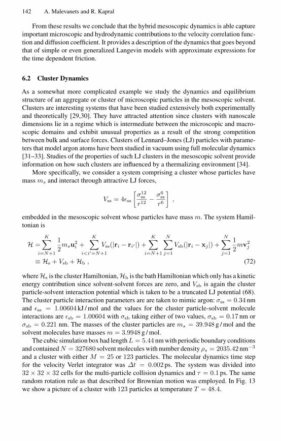
and a cluster with either M = 25 or 123 particles. The molecular dynamics time stepfor the velocity Verlet integrator was ∆t = 0.002 ps. The system was divided into32 × 32 × 32 cells for the multi-particle collision dynamics and τ = 0.1 ps. The samerandom rotation rule as that described for Brownian motion was employed. In Fig. 13we show a picture of a cluster with 123 particles at temperature T = 48.4.


Fig. 13. Picture of a M = 123 atom cluster in the mesoscopic solvent. The cluster particles aredepicted as large atoms while the solvent atoms are small. Only solvent molecules close to thecluster surface are shown in the figure for clarity

The cluster structure can be described by the radial distribution function for clusterand solvent molecules relative to the center of mass of the cluster,

gCM−α(r) =1

4πr2ρα

⟨ Nα∑

i

δ(|xi −RCM| − r)⟩,

where α = s or b designates a cluster or solvent molecule, RCM is the center ofmass of the cluster and ρα is the number density of cluster or solvent molecules. Hereρs = σ−3

ss = 25.44 nm−3.For clusters in vacuum gCM−c(r) shows liquid-like distributions of cluster particles

and structural ordering within the clusters [32,33]. The cluster structure is modifiedwhen it is embedded in the mesoscopic solvent and the modifications depend on thecluster-solvent interactions. We fix εsb = εss and vary σsb. The M = 25 cluster radialdistribution functions are shown in Fig. 14 (left) and (right) for σsb = 0.17 and σsb =0.221, respectively. The radial distribution functions gCM−s(r) for the solvent moleculesrelative to the cluster center of mass are also shown in the figure. The structures ofthe radial distribution functions are similar in vacuum and in the mesoscopic solventfor σsb = 0.17 nm but are quite different for σsb = 0.221 nm where the cluster iscompressed and adopts a solid-like configuration.

This difference is signalled in the structure of the solvent molecule-cluster particledistributions. For σsb = 0.17 the solvent molecules are able to penetrate into the cluster.For σsb = 0.221 they are not able to do so and the solvent provides a larger external forceon the cluster which compresses it and induces a solid-like structural configuration.

The center of mass diffusion coefficients of the clusters can be analyzed using theapproximate formula (71) presented in the previous subsection. Since the cluster is acomposite object we can determine its effective radius R from the radial distributionfunction. For theM = 25 cluster with σsb = 0.17 we find R ≈ 2.25. Furthermore, thecentral LJ forces now act on the individual cluster atoms so for macroscopic sizes thecluster will appear to have stick boundary conditions. Given these facts, we may estimateD for the cluster and compare the value with that obtained from the simulation of the


0 0.5 1 1.5 2 2.5r*

0

0.5

1

1.5

g(r)

0 0.5 1 1.5 2 2.5r*

0

2

4

6

8

g(r)

Fig. 14. Radial distribution function gCM−c(r) versus r∗ for σsb = 0.221 nm (left) and σsb =0.17 nm (right) for M = 25 (T = 40.33) clusters in the mesoscale solvent (solid lines); vacuumcluster (dotted lines). Also shown is the solvent radial distribution function gCM−s(r) (dashedlines)

mean square displacement of the cluster. We find, in units of cm2 / s,D0 = 2.8× 10−7,Dh = 7.8×10−7, so thatD(theory) ≈ 1.1×10−6. The simulation result isD(sim) =9.6× 10−7.

6.3 Polymer Dynamics

The dynamics of a long polymer chain in solution is determined by macroscopic prop-erties of the solvent [35] rather than the microscopic details of the chain-solvent in-teractions. Indeed, time scale separation between the microscopic collision processesand hydrodynamic flows that define the long time evolution of a polymer chain makesdirect simulations of polymer dynamics a challenging task. Therefore, in simulations, itis suitable to replace molecular solvents with mesoscale models [36–38].

Multi-particle collision dynamics can be adapted to model polymer flows [38]. Inone version of the model the system is extended to include a polymer chain and “inert”solvent. The polymer chain itself is modelled using standard molecular dynamics. Thearchitecture of the chain and the interactions within it can be varied. The free-streamingpropagation step is modified to include evolution of the chain by integrating the chainequations of motion on the time interval τ ,

(X(M)(t+ τ),V(M)(t+ τ)) = eiLτ (X(M)(t),V(M)(t)) . (73)

Here (X(M)(t),V(M)(t)) denotes a set velocities and coordinates of a polymer chainwith M monomers and iL is defined by the relation iLu = H, u for any dynamicalvariable u. The HamiltonianH of the system is given by

H =∑

i∈ solvent

12miv2

i +∑

i∈ chain

12MiV2

i +∑

i≤j∈ chain

Uij(Ri,Rj) . (74)

During the propagation step the system evolves according to Newton’s equation ofmotion. For chain atoms (73) is solved by integration of the equation of motions of a


Fig. 15. Snapshot of a chain configuration showing a few of the surrounding mesoscopic solventmolecules

free chain using the Verlet algorithm

Ri(t+∆t) = Ri(t) +∆tVi(t) +(∆t)2

2miFi

(Ri(t)

),

Vi(t+∆t) = Vi(t) +∆t

2Mi

[

Fi

(Ri(t)

)+ Fi

(Ri(t+∆t)

)]

,(75)

with a time step of∆t to evolve the positions and velocities in the MD step. As no forceis exerted on the solvent between collision steps we propagate solvent particles with atime step ∆t = 1.

To capture hydrodynamic interactions between molecules comprising the chain itis necessary to add chain-solvent interactions. This can done within the multi-particlecollision scheme approach without destroying the conservation laws. To this end, duringthe collision step an additional collision step (2) exchanging momenta and energies ofthe polymer beads and solvent particles in the same cell is performed. By choosing asuitable class of rotation matrices ω one may tune the bead-solvent friction coefficient.A snapshot of a polymer configuration in the mesoscopic solvent is shown in Fig. 15.

The numerical results of simulations were shown to agree well with an equation ofmotion for a chain which assumed a linear coupling to the velocity of the surround-ing fluid via viscous friction [38]. Simulations demonstrated that the velocity-velocitycorrelation function comprises two contributions; an initial exponential decay result-ing from Brownian collisions of monomers with uncorrelated solvent molecules and,at longer times, a hydrodynamic contribution as monomers interact via hydrodynamicmodes propagated through the solvent. Analysis of chain diffusion coefficient given bythe integral of the velocity-velocity correlation function demonstrated Zimm scalingD ∼ R−1

G for the hydrodynamic contribution to the diffusion constant.


6.4 Complex Fluids

The multi-particle collision model has been extended to the treatment of binary im-miscible fluids with a conserved order parameter [39]. The extension is based on theRothman–Keller model [40] for immiscible lattice gases. The original Rothman–Kellermodel considers two kinds of particle, called red and blue, and introduces two fieldsrelated to the colors of the particles: A color flux and a color field. The immisciblelattice-gas model is constructed to account for cohesion in real fluids arising from shortrange attractive intermolecular forces by allowing particles in neighboring sites to influ-ence the configuration of particles at a chosen site. This is accomplished by constructingcollision rules where the “work” performed by the color flux against the color field is aminimum.

This idea can be transcribed to the multi-particle collision rule by altering the natureof the rotation operator that effects the collisions in a cell [39]. Again, we let ξν denotethe coordinate of the center of cell ν, and introduce a characteristic functionHi(ξν) forparticle i in cell ν which takes the value +1 if the particle is red and -1 if the particle isblue. Using this notation the color flux is defined as

qν =n(ξν)∑

i=1

Hi(ξν)(v′i − Vξν

) , (76)

where n(ξν) is the number of particles in cell ν. This is the color-weighted relativevelocity of the particles in cell ν. The color field is a color gradient arising from thecolor differences in neighboring cells,

fν =∑

ν′∈N (ν)

wνν′ ξνν′

n(ξν′ )∑

i=1

Hi(ξν′) , (77)

where ξνν′ is a unit vector along the relative separation between cells ν and ν′, thatis ξνν′ = (ξν − ξν′)/|ξν − ξν′ |, and N (ν) denotes the cells neighboring cell ν. Theweight function wνν′ is taken to be wνν′ = |ξν − ξν′ |−1.

Given these definitions, the rotation matrix, ωcν , for multi-particle collisions in a cell

with coordinates ξν is constructed so that the rotated color flux lies along the color field,fν = ωc

ν qν . If we let hν = fν × qν , which is normal to both the color flux and colorfield vectors, the rotation operator effects a rotation of qν by an angle θ about hν , whereθ is the angle between qν and fν , cos θ = fν · qν . The multi-particle collision rule againtakes the form, vi = Vξ + ωc(v′

i − Vξ), where now, from (5),

ωc(v′i − Vξ) = hh · (v′

i − Vξ) + (I− hh) · (v′i − Vξ) cos θ − h× (v′

i − Vξ) sin θ .(78)

This rule has been used to simulate phase segregation in binary fluids in two and three di-mensions [39]. Simulations on the model have shown that Laplace’s law for the pressuredifference inside and outside a droplet of radius R,∆p = 2σ/R, where σ is the surfacetension, is satisfied and that this generalization of the collision rule reproduces the main


features of phase segregation dynamics. However, we note that this generalization nolonger preserves phase space volumes and is not time reversible. As a result the equi-librium distribution is not Maxwellian. The model has also been extended to includesurfactant molecules so that microemulsions may be simulated using such dynamics[41,42].

7 Conclusion and Perspectives

The multi-particle collision model provides a simple way to simulate the dynamics offluids at the mesoscopic level. We have demonstrated that it possesses some basic ingre-dients which are desirable in such models: Mass, momentum and energy are conserved,the equilibrium distribution is Maxwellian, an H-theorem exists and the full set of hy-drodynamic equations are obtained on long distance and time scales. Consequently,the model should find applications to problems in fluid flow and turbulence, especiallyin complex geometries where solutions of the Navier–Stokes equation are difficult. Inthis case it may provide an approach that complements DSMC, lattice-gas or latticeBoltzmann methods.

The hybrid mesoscopic multi-particle collision model marries full molecular dynam-ics of embedded particles (solutes) with a mesoscopic treatment of the solvent. We haveshown that this hybrid scheme is able to capture essential features of both microscopicand hydrodynamic contributions arising from coupling between the solute and solventdegrees of freedom. The model is flexible enough to allow one to model large colloidalparticles by using bounce-back [8] and other suitable generalizations of the collisionrule to account for solid objects [39,43] or molecular degrees of freedom using explicitsolute-solvent intermolecular potentials. The simple applications presented above havedemonstrated the utility of this approach for the Brownian motion of molecules, molec-ular aggregates and polymer molecules in solution. This hybrid approach is likely toprovide a promising route to investigate the dynamics of large biopolymers in solutionwhere both specific details of solute-solvent forces and hydrodynamic solvent effectsplay important roles.

The development of the multi-particle collision model is still at an early stage. Fur-ther generalizations of the model to more complex situations; for example, molecularfluids, chemically reacting flows and more complex systems are possible. The modelshould not only provide a means to simulate efficiently complex systems and help bridgemicroscopic and macroscopic time scales but should also permit one to understand someof the important features of solute-solvent dynamics without recourse to full moleculardynamics of very large systems.

Acknowledgements

This work was supported in part by a grant from the Natural Sciences and EngineeringResearch Council of Canada.


References

1. D.H. Rothman, S. Zaleski: Lattice-Gas Cellular Automata: Simple Models of Complex Hy-drodynamics (Cambridge University Press, Cambridge 1997)

2. J.-P. Rivet, J.-P. Boon: Lattice Gas Hydrodynamics (Cambridge University Press, Cambridge2001)

3. I. Pagonabarraga: Lattice Boltzmann Modeling of Complex Fluids: Colloidal Suspensionsand Fluid Mixtures, Lect. Notes Phys. 640, 275 (2004)

4. For a review, see, S. Chen, G. Doolen: Ann. Rev. Fluid Mech. 30, 329 (1998)5. L. S. Luo: Phys. Rev. E 62, 4982 (2000)6. S. Succi: The Lattice Boltzmann Equation – For Fluid Dynamics and Beyond (Clarendon

Press, Oxford 2001)7. A. Malevanets, R. Kapral: J. Chem. Phys. 110, 8605 (1999)8. A. Malevanets, R. Kapral: J. Chem. Phys. 112, 7260 (2000)9. G. A. Bird: Molecular Gas Dynamics (Clarendon Press, Oxford 1976); G. A. Bird: Comp. &

Math. with Appl. 35, 1 (1998)10. The multi-particle collision rule was first introduced in the context of a lattice model with a

stochastic streaming rule in: A. Malevanets, R. Kapral: Europhys. Lett. 44, 552 (1998)11. R. Zwanzig: J. Chem. Phys. 33, 1338 (1960)12. H. Mori: Prog. Theor. Phys. 33, 423 (1965)13. Related derivations for lattice-gas automata have been carried out in D. d’Humieres, B. Has-

slacher, P. Lallemand, Y. Pomeau, J.-P. Rivet: Complex systems 1, 839, (1987); M. H. Ernst.In: Microscopic Simulations of Complex Hydrodynamics Phenomena, ed. by M. Mareschal,B. Holian (Plenum Press, New York 1992) p. 153

14. G. K. Batchelor: J. Fluid Mech. 74, 1 (1976)15. T. Ihle, D. M. Kroll: Phys. Rev. E 63, 020201 (2001)16. A. Lamura, G. Gompper, T. Ihle, D. M. Kroll: Europhys. Lett. 56, 768 (2001)17. A. Lamura, G. Gompper, T. Ihle, D. M. Kroll: Europhys. Lett. 56, 319 (2001)18. W. C. Swope, H. C. Andersen, P. H. Berens, K. R. Wilson: J. Chem. Phys. 76, 673 (1982); M.

Tuckerman, B. J. Berne, G. J. Martyna: J. Chem. Phys. 97, 1990 (1992)19. A. Einstein: Investigations on the Theory of Brownian Movement, ed. by R. Furth (Dover,

New York 1956)20. S. Chandrasekhar: Rev. Mod. Phys. 15, 1 (1943)21. R. Kubo: The Fluctuation-Dissipation Theorem. In: Many-Body Problems, ed. by W. E. Parry

et al. (W. A. Benjamin, New York 1969), p. 23522. M. Tokuyama, I. Oppenheim: Physica A 94, 501 (1978)23. B. J. Alder, T. E. Wainwright: Phys. Rev. Lett. 18, 988 (1967)24. J. R. Dorfman, E. G. D. Cohen: Phys. Rev. Lett. 25, 1257 (1970)25. K. Kawasaki: Prog. Theor. Phys. 45, 1691 (1971)26. R. Zwanzig, M. Bixon: Phys. Rev. A 2, 2005 (1970)27. L. D. Landau, E. M. Lifshitz: Fluid Mechanics (Pergamon Press, New York 1959)28. J. T. Hynes, R. Kapral, M. Weinberg: J. Chem. Phys. 70 1456 (1979)29. A. W. Castleman, Jr., R. G. Keese: Chem. Rev. 86, 589 (1986); Annu. Rev. Phys. Chem. 37,

525 (1986); Science 241, 36 (1988); A. W. Castleman, Jr., S. Wei: Ann. Rev. Phys. Chem. 45,685 (1994)

30. R. S. Berry, T. L. Beck, H. I. Davis, J. Jellinek: Adv. Chem. Phys. 70, 75 (1988); M. Y. Hahn,R. L. Whetten: Phys. Rev. Lett. 61, 1190 (1988); H.-P. Cheng, X. Li, R. L. Whetten, R. S.Berry: Phys. Rev. A 46, 791 (1992)

31. J. D. Honeycutt, H. C. Andersen: J. Phys. Chem. 91, 4950 (1987)32. B. G. Moore, A. A. Al-Quraishi: Chem. Phys. 252, 337 (2000)


33. A. S. Clarke, R. Kapral, B. Moore, G. Patey, X.-G. Wu: Phys. Rev. Lett. 70, 3283 (1993); A.S. Clarke, R. Kapral, G. Patey: J. Chem. Phys. 101, 2432 (1994)

34. S.-H. Lee, R. Kapral: Physica A 298, 56 (2001)35. M. Doi: Introduction to Polymer Physics (Clarendon Press, Oxford 1996)36. P. Ahlrichs, B. Dunweg: J. Chem. Phys. 111, 8225 (1999)37. Y. Kong, C. W. Manke, W. G. Madden, A. G. Schlijper: J. Chem. Phys. 107, 592 (1997)38. A. Malevanets, J. M. Yeomans: Europhys. Lett. 52, 231 (2000)39. Y. Hashimoto, Y. Chen, H. Ohashi: Comput. Phys. Commun. 129, 56 (2000)40. D. H. Rothman, J. M. Keller: J. Stat. Phys.52, 1119 (1988)41. Y. Inoue, Y. Chen, H. Ohashi: Colloids and Surfaces A 201, 297 (2002)42. T. Sakai, Y. Chen, H. Ohashi: Phys. Rev. E 65, 031503 (2002)43. T. Sakai, Y. Chen, H. Ohashi: J. Stat. Phys. 107, 85 (2002)

Documents

Mesoscopic Multi-particle Collision Model for Fluid Flow ...rkapral/Papers/meso_rev.pdf · It is well known that the hydrodynamic equations of motion are a macroscopic ... Mesoscopic