Mesoscale Correlation Length Scales from NSCAT and … · Mesoscale Correlation Length Scales from NSCAT and Minimet Surface Wind ... Paciﬁc Gyre Corporation, Carlsbad, ... rador

APRIL 2003 513M I L L I F F E T A L .

q 2003 American Meteorological Society

Mesoscale Correlation Length Scales from NSCAT and Minimet Surface WindRetrievals in the Labrador Sea

R. F. MILLIFF

Colorado Research Associates, NorthWest Research Associates, Boulder, Colorado

P. P. NIILER

Scripps Institution of Oceanography, La Jolla, California

J. MORZEL

Colorado Research Associates, Boulder, Colorado

A. E. SYBRANDY

Pacific Gyre Corporation, Carlsbad, California

D. NYCHKA AND W. G. LARGE

National Center for Atmospheric Research, Boulder, Colorado

(Manuscript received 29 November 2001, in final form 1 August 2002)

ABSTRACT

Observations of the surface wind speed and direction in the Labrador Sea for the period October 1996–May1997 were obtained by the NASA scatterometer (NSCAT), and by 21 newly developed Minimet drifting buoys.Minimet wind speeds are inferred, hourly, from observations of acoustic pressure in the Wind-Speed ObservationThrough Ambient Noise (WOTAN) technology. Wind directions are inferred from a direction histogram, alsoaccumulated hourly, as determined by the orientation of a wind vane attached to the surface floatation. Effectivetemporal averaging of acoustic pressure (20 min), and the interval over which the direction histogram is ac-cumulated (160 s), are shown to be consistent with low-pass filtering to preserve mesoscale time- and space-scale signals in the surface wind. Minimet wind speed and direction retrievals in the Labrador Sea were calibratedwith collocated NSCAT data. The NSCAT calibrations extend over the full field lifetimes of each Minimet (90days on average). Wind speed variabilities of O(5 m s21) and wind direction variabilities of O(408) are evidenton timescales of one to several hours in Minimet time series. Wind speed and direction rms differences versusspatial separation comparisons (from 0 to 400 km) for the NSCAT and Minimet records demonstrate similarrms differences in wind speed as a function of spatial separation, but O(208) larger rms differences in Minimetdirection. These differences are consistent with spatial smoothing effects in the median filter step for winddirection retrievals within the NSCAT swath. Zonal and meridional surface wind components are constructedfrom the calibrated Minimet wind speed and direction dataset. Rms differences versus spatial separation forthese components are used to estimate mesoscale spatial correlation length scales of 250 and 290 km in thezonal and meridional directions, respectively.

1. Introduction

The purposes of this paper are twofold: first, to in-troduce the surface wind observation capabilities ofMinimet drifter systems as demonstrated in their firstdeployments in the Labrador Sea; and second, to dem-onstrate how Minimet observations, in concert with co-

Corresponding author address: Dr. Ralph F. Milliff, Colorado Re-search Associates, 3380 Mitchell Ln, Boulder, CO 80301-5410.E-mail: [email protected]

incident scatterometer data, can recover spatial prop-erties of the mesoscale marine surface wind field.

Nested levels of organization are often defined tocharacterize geophysical fluid motions in terms of pair-ings of time- and space scales that are observed to occurin natural systems. The wind field at the surface of theocean is amenable to characterizations of this kind.Three levels of organization of the surface wind fieldare relevant to this study; namely, the microscale, themesoscale, and the synoptic scale.

Synoptic-scale features of the surface wind field in

514 VOLUME 20J O U R N A L O F A T M O S P H E R I C A N D O C E A N I C T E C H N O L O G Y

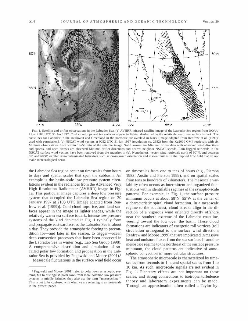
FIG. 1. Satellite and drifter observations in the Labrador Sea. (a) AVHRR infrared satellite image of the Labrador Sea region from NOAA-12 at 2103 UTC 30 Jan 1997. Cold cloud tops and ice surfaces appear in lighter shades, while the relatively warm sea surface is dark. Thecoastlines for Labrador in the southwest and Greenland in the northeast are overlaid in black [image adapted from Renfrew et al. (1999);used with permission]. (b) NSCAT wind vectors at 0052 UTC 31 Jan 1997 (revolution no. 2382) from the Ku2000 GMF retrievals with sixMinimet observations from within 18–53 min of the satellite image. Solid arrows are Minimet drifter data with observed wind directionsand speeds, and open arrows are observed Minimet drifter directions and nearest-neighbor NSCAT speeds. Rain-flagged retrievals in theNSCAT surface wind vectors have been removed from the snapshot in (b). Nonetheless, vector wind retrievals north of 608N, and between558 and 608W, exhibit rain-contaminated behaviors such as cross-swath orientation and discontinuities in the implied flow field that do notmake meteorological sense.

the Labrador Sea region occur on timescales from hoursto days and spatial scales that span the subbasin. Anexample is the basin-scale low pressure system circu-lations evident in the radiances from the Advanced VeryHigh Resolution Radiometer (AVHRR) image in Fig.1a. This particular image captures a deep low pressuresystem that occupied the Labrador Sea region on 30January 1997 at 2103 UTC [image adapted from Ren-frew et al. (1999)]. Cold cloud tops, ice, and land sur-faces appear in the image as lighter shades, while therelatively warm sea surface is dark. Intense low pressuresystems of the kind depicted in Fig. 1 typically formand propagate eastward across the Labrador Sea in abouta day. They provide the atmospheric forcing to precon-dition for—and later in the season, to trigger—oceandeep convection processes that have been observed inthe Labrador Sea in winter (e.g., Lab Sea Group 1998).A comprehensive description and simulation of so-called polar low formation and propagation in the Lab-rador Sea is provided by Pagowski and Moore (2001).1

Mesoscale fluctuations in the surface wind field occur

1 Pagowski and Moore (2001) refer to polar lows as synoptic sys-tems, but to distinguish polar lows from more common low pressuresystems in middle latitudes they also use the term ‘‘mesocyclone.’’This is not to be confused with what we are referring to as mesoscalein the present paper.

on timescales from one to tens of hours (e.g., Pierson1983; Austin and Pierson 1999), and on spatial scalesfrom tens to hundreds of kilometers. The mesoscale var-iability often occurs as intermittent and organized fluc-tuations within identifiable regimes of the synoptic-scalepatterns. For example, in Fig. 1, the surface pressureminimum occurs at about 588N, 558W at the center ofa characteristic spiral cloud formation. In a mesoscaleregime to the southeast, cloud streaks align in the di-rection of a vigorous wind oriented directly offshorenear the southern extreme of the Labrador coastline,veering toward the low over the basin. These cloudformations are indicators of energetic roll vortices (rollcirculation orthogonal to the surface wind direction;Renfrew and Moore 1999) that are implicated in massiveheat and moisture fluxes from the sea surface. In anothermesoscale regime to the northeast of the surface pressureminimum, the cloud patterns are indicative of atmo-spheric convection in more cellular structures.

The atmospheric microscale is characterized by time-scales from seconds to 1 h, and spatial scales from 1 to10 km. As such, microscale signals are not evident inFig. 1. Planetary effects are not important on thesescales, and strong connections to isotropic turbulencetheory and laboratory experiments can be made.Through an approximation often called a Taylor hy-


pothesis microscale fluctuations in time can be inter-preted to imply microscale spatial dimensions, and viceversa (e.g., Lumley and Panofsky 1964). That is Tu øL, where T is the period, u is a characteristic microscalevelocity, and L is a microscale length scale. Spectralproperties of the microscale surface layer wind are quan-tified and generalized in Kaimal et al. (1972). Whilethese properties derive from measurements over land,the authors demonstrate that the normalized spectrafrom over-water field experiments exhibit similar be-haviors. Importantly, Kaimal et al. (1972) demonstratea peak in surface velocity spectra (longitudinal andtransverse components), occurring at higher frequenciesquite apart from the energy at mesoscale frequencies.This gives rise to the widespread notion of a spectralgap between the microscale and mesoscale energy inthe surface wind field.

Surface wind observing systems can be placed in thecontext of these levels of organization. In this paper wewill describe averaging of samples at microscale fre-quencies in Minimet drifters over timescales coincidentwith the spectral gap, as a means of low-pass filteringto isolate the mesoscale. Also, we will describe cali-brations of Minimet wind speed and direction retrievalswith near-neighbor NSCAT retrievals. We will show thatthese calibrations were necessary to extract geophysicalinformation from the Minimet wind observations andset the mesoscale signal from Minimet data in its propersynoptic context.

The advent of calibrated satellite scatterometers hasmade possible continuous observation of synoptic pat-terns of the surface vector wind over large regions ofWorld Ocean [see Jones et al. (1982) for a Seasat ex-ample; see also the National Aeronautics and Space Ad-ministration (NASA) scatterometer (NSCAT) papersfollowing O’Brien (1999)]. Following the launch of theNSCAT instrument aboard the ADEOS-I satellite plat-form in August 1996, comparisons and calibrations weremade using a variety of wind retrieval algorithms within situ surface wind observations from moored buoys(e.g., Dickinson et al. 2001; Freilich and Dunbar 1999),research ships (Bourassa et al. 1997), and numericalweather prediction products (Liu et al. 1998; Atlas etal. 1999). These comparisons and calibrations, and thederivation of so-called geophysical model functions(GMFs) to retrieve vector wind information from radarbackscatter, all focus on accurate reproduction of syn-optic-scale surface winds. While the within-swath res-olution for NSCAT is sufficient to resolve mesoscalespatial variability, it is the synoptic scales that are mostapparent in the wind retrievals. Figure 1b demonstratesthe surface wind retrievals from NSCAT within 4 h ofthe AVHRR image (Fig. 1a). The synoptic-scale cir-culation is consistent with the polar low that fills theLabrador Sea subbasin.

The spatial properties of the mesoscale surface windvariability over the ocean are very difficult to observeover spatial scales that approach the synoptic systems

within which the mesoscale is embedded. A single polar-orbiting spaceborne system is incapable of achievingmesoscale temporal resolution uniformly over the globe(Milliff et al. 2001; Schlax et al. 2001). Spatial infor-mation regarding the mesoscale surface wind cannot bedirectly obtained from operational moored buoys [e.g.,Tropical Atmosphere Ocean (TAO), National Data BuoyCenter, etc.] as these are not deployed in mesoscalearrays. Neither can available ship observations be usedsince research vessel observations generally occur alongstraight cruise tracks, often on timescales longer thanmesoscale. Weller et al. (1983) report that intercalibra-tion issues for a mesoscale array of in situ surface windsensors precluded detection of spatial properties of themesoscale wind field during the Joint Air–Sea Inter-action (JASIN) experiment.

In this paper we introduce the Minimet wind observ-ing system. We show that using scatterometer wind ob-servations, the Minimet dataset can be calibrated to pro-vide first estimates of the spatial length scales of themesoscale surface wind field for the Labrador Sea inwinter. The NSCAT system and data for our study periodare reviewed in section 2. The Minimet design and ob-serving system heritage are introduced in section 3. Alsoin section 3, we review field calibrations and sampledata from the Minimet wind observing systems de-ployed in the Labrador Sea. More detailed informationconcerning Minimet drifter design, data processing, andpredeployment calibrations are provided in an appendix.In section 4 we compare the Labrador Sea Minimetwinds with coincident NSCAT wind retrievals to dem-onstrate a mesoscale signal in the wintertime surfacewinds that is largely removed by NSCAT retrieval al-gorithms. First estimates of the spatial properties of themesoscale surface wind field on the Labrador Sea inwinter are derived to conclude this paper.

2. NSCAT wind retrievals in the Labrador Sea

The NSCAT mission from 15 September 1996through 29 June 1997 spans the winter season of ourstudy. A complete overview of the NSCAT instrumentand mission is available from Naderi et al. (1991).NSCAT was a fan beam scatterometer that illuminatedthe sea surface with radar energy at a frequency of 14GHz. Backscatter signals were detected from a varietyof incidence and azimuth angles, and for horizontal andvertical radar polarizations, along three antennas (fore,mid, and aft beams) on each side of the NSCAT in-strument. The incidence angle, azimuth angle, and po-larization diversity accounted for complicated patternsof overlapping radar footprints at the surface [see Fig.1 in Jones et al. (1999)]. These returns are compositedover wind vector cell (WVC) areas of 25 km 3 25 km.The composite backscatter from each WVC is relatedto a wind vector by inverting a GMF that relates thenormalized radar backscatter to wind speed and winddirection, as well as other radar and geometric param-


eters. The radar backscatter in the NSCAT frequencyrange can be affected by heavy rain. Raindrops attenuateand backscatter the radar signal, as well as change theroughness of the sea surface. Wind vectors are retrievedfor each WVC over the ice-free ocean and where theradar backscatter is not contaminated by rain. Globally,NSCAT sampled about 90% of the ice-free global oceanevery 2 days.

Because of inherent measurement noise, typical GMFinversions yield several possible, or ambiguous, vectorwinds for a given WVC. Each ambiguity is assigned alikelihood in the GMF inversion algorithm. The rangeof wind speed ambiguities is found to be small, but therange of wind direction ambiguities can be large, witha significant number of direction ambiguities differingby 1808; the so-called upwind/downwind ambiguity. Amedian filter method (Shultz 1990; Shaffer et al. 1991;Gonzales and Long 1999) is used to iteratively selectamong ambiguities by finding the closest vector to themedian of selected vectors in several neighboringWVCs. The iterative process is often initiated by findingthe direction ambiguities closest to coarse-resolutionweather center analyses [so-called numerical weatherprediction (NWP) nudging].

The development and testing of geophysical modelfunctions, including the median filter step, for scatter-ometer systems is an area of ongoing research (Wentzet al. 1984, 1986; Freilich and Challenor 1994; Freilichand Dunbar 1993a,b; Stoffelen and Anderson 1997;Gonzales and Long 1999; Mejia et al. 1999; Wentz andSmith 1999; Brown 2000). In our analyses, we haveused the wind vector retrievals based on the NSCAT–Ku2000 GMF developed by Wentz and Smith (1999)(available online at Remote Sensing Systems at ftp://ftp.ssmi.com). Only the highest quality retrievals havebeen used, which exclude data identified as rain con-taminated as well as retrievals with poor GMF fits. TheNSCAT–Ku2000 retrievals correct for small global di-rectional biases identified in prior retrieval products.2

Wentz and Smith (1999) validate the NSCAT–Ku2000wind speed and direction retrievals in comparisons withobservations from moored ocean buoys, and with oceansurface wind analyses from the National Centers forEnvironmental Prediction. Average speed biases werewithin 1 m s21 with an rms of 2 m s21. Wind directionbiases are within 108 of the validation data, with an rmsdirection variability of 208.

NSCAT coverage at latitudes 508–658N, in the Lab-rador Sea region, was excellent. NSCAT orbited theearth about 14 times per day, with exact repeat orbitsevery 41 days (NASA Scatterometer Project 1998). The

2 The wind direction distribution function for NSCAT wind retriev-als over the entire globe, based on the NSCAT-2 GMF from the NASAJet Propulsion Laboratory, contained small artifacts associated withthe antenna orientations. These were corrected in the NSCAT–Ku2000 GMF, which came later. The results of our study are notsensitive to these small effects.

NSCAT swath spans 600 km on either side of the sub-satellite ground track, separated by a 400-km gap incoverage centered at nadir. Each swath is partitionedinto 25 km 3 25 km WVC; that is, 48 WVC in thecross-track direction. The NSCAT overflights of theLabrador Sea occurred near 0000 UTC (ascending or-bital tracks) and 1400 UTC (descending orbital tracks).The Labrador Sea orientation is such that swath cov-erage spans the entire basin for a large subset of theascending orbits in the region. Frequently, successivedescending orbits overlap in the Labrador Sea regionsuch that dense sampling of the surface wind field occurswithin a 101-min time window (an example is depictedin Fig. 6, which will be discussed below).

To the extent that neighboring WVC wind directionsinfluence the local wind direction ambiguity selection,the median filter operates as a spatial smoother on winddirection variability within the NSCAT swath. Since thewind speed ambiguities for each WVC do not differwidely, the spatial smoothing effect on speed is lesspronounced. Thus, the 25-km WVC spacing within theNSCAT swath might be sufficient to resolve mesoscalespatial variability in wind speed, but spatial resolutionof wind direction variability within the NSCAT swathis coarsened by the median filter. We will quantify theseissues by comparison with Minimet drifter spatial res-olutions for wind speed and direction in section 4.

3. Minimet observations of the surface wind fieldin the Labrador Sea

Design considerations in the development of surfacewind observation systems for the Labrador Sea Minimetdrifter deployments were driven in part by the goals ofthe Deep Convection Experiment as described by theLab Sea Group (1998). The Minimet drifter wind ob-servation systems were designed to be capable of reli-able observations and remote communications for anentire winter season. Surface wind speed, wind direc-tion, and ancillary data were obtained at mesoscale res-olution under sustained conditions of very high windsand rough seas. The Labrador Sea Minimet drifter pro-totypes integrate advanced technologies that existedseparately in drifter mechanical and electronic compo-nents, and in moored wind observing systems and com-pass technologies. Integrating these technologies in mul-tiple durable Lagrangian packages for simultaneous de-ployments posed new challenges in data processing andremote communications as well. In this section we focuson the field calibrations and surface wind datasets toemerge from the Labrador Sea deployment. The upper-ocean response part of the Labrador Sea Minimet de-ployments will be described elsewhere. At several pointsin the discussion, the interested reader is referred to anappendix that details aspects of the Minimet wind ob-servation system design and engineering calibrationsthat are critical to the introduction of this new instrumenttechnology.


FIG. 2. Minimet drifter configuration. Schematics depicting thefully deployed Minimet drifter configuration including surface andsubsurface floatation, the hydrophone cage, and a holey-sock drogue;an expanded view of the WOTAN instrument configuration; and anexpanded diagram of the surface floatation components.

We will show that spatial properties of the surfacemesoscale wind field are accessible from multiple [e.g.,O(10)] in situ drifting Minimets that coincide withO(100) NSCAT overflights of the study region. De-ploying multiple in situ systems constrains costs suchthat construction, deployment, and calibration proce-dures for each drifter must be inexpensive and repeat-able. For example, drifter recovery and individual po-stcalibrations are not practical. Requiring long field life-times [e.g., O(100 days)] for each drifter constrainspower consumption, thereby limiting sensor designs,and sampling and communication duty cycles.

The Minimet drifter mechanical configuration is di-agrammed in Fig. 2. Some of the Minimet drifter designand wind observing system heritage is already evidentin the figure. Drifter structure, floatation, and droguedesigns are direct descendants of the World Ocean Cir-culation Experiment–Tropical Oceans and Global At-mosphere (WOCE–TOGA) Lagrangian drifter systemsdescribed by Sybrandy and Niiler (1991). The acoustichydrophone component is representative of the WindObservation Through Ambient Noise (WOTAN) tech-nology for wind speed observations in harsh conditionsthat had been demonstrated for moorings by Vagle etal. (1990), and in drifter systems for more benign en-vironments by Nystuen and Selsor (1997). Previous ob-

servations of wind direction from drifting systems inrough seas have been made from large platforms thatprecluded simultaneous ocean current estimates. Suchobservations compare favorably with conventionalmoored buoys, and operational analysis from numericalweather prediction; 658 in the mean, ,158 standarddeviations after discarding outliers (Large et al. 1995).As in the case of Minimet, these prior observations de-rive from vanes fixed to the floatation elements, and theuse of histograms of wind direction to determine themost common direction. A primary Minimet innovationwas to overcome the major technical difficulty of fol-lowing the surface current while still remaining abovethe surface for time periods long enough to amply sensethe surface wind (Niiler et al. 1987, 1995). The windvane addition to the drifter spherical surface floatationand electronics housing is the external component ofthe new wind direction observing system developed forthe Labrador Sea Minimet.

Sampling and communications configurations forMinimet drifters evolved from high-resolution, powerconsumptive systems used to calibrate engineering mod-el Minimet drifters in the laboratory and in sea trialsoff California; to the hardened, low-power Minimet sys-tems deployed in the Labrador Sea. The Labrador Seasystems transmit data in near–real time via System AR-GOS satellite remote communications resources. Min-imet observational records are refreshed every hour, andthe most recent data record is transmitted nominallyevery 90 s. The System ARGOS coverage of the Lab-rador Sea region was such that, on average, hourly datawere received about 14 times per day.

Wind direction observations derive from histogramsof the wind vane orientation, in 58 bins, as sampled at1 Hz for 160 s every hour. Details of the predeploymentMinimet wind direction calibration are provided in theappendix. Under low- to medium-strength wind con-ditions, rms wind direction differences are between 68and 88 for drifters within a few hundred meters of eachother. Additional field calibrations for Minimet winddirection retrievals in the Labrador Sea deployment aredescribed in section 3a below.

Minimet wind speed observations derive from acous-tic pressure data collected by the WOTAN hydrophoneand averaged in four batches of 5 min each, over a 20-min period, every hour. Within each batch, the acousticpressure signal is sampled for 30 s each minute, andaveraged. As detailed in the appendix, the Minimet windspeed calibration differs from the attempts by Vagle etal. (1990) for absolute wind speed calibration usingWOTAN systems. Instead, a relative calibration withNSCAT is maintained over the field lifetime of eachdrifter in the Labrador Sea. Absolute calibration of WO-TAN systems has not proven feasible when deploymentlocations differ (Vakkayil et al. 1996), or for multiplehydrophone systems in the same location (appendix).

While effective averaging times for Minimet windspeed (acoustic pressure amplitudes averaged over 20


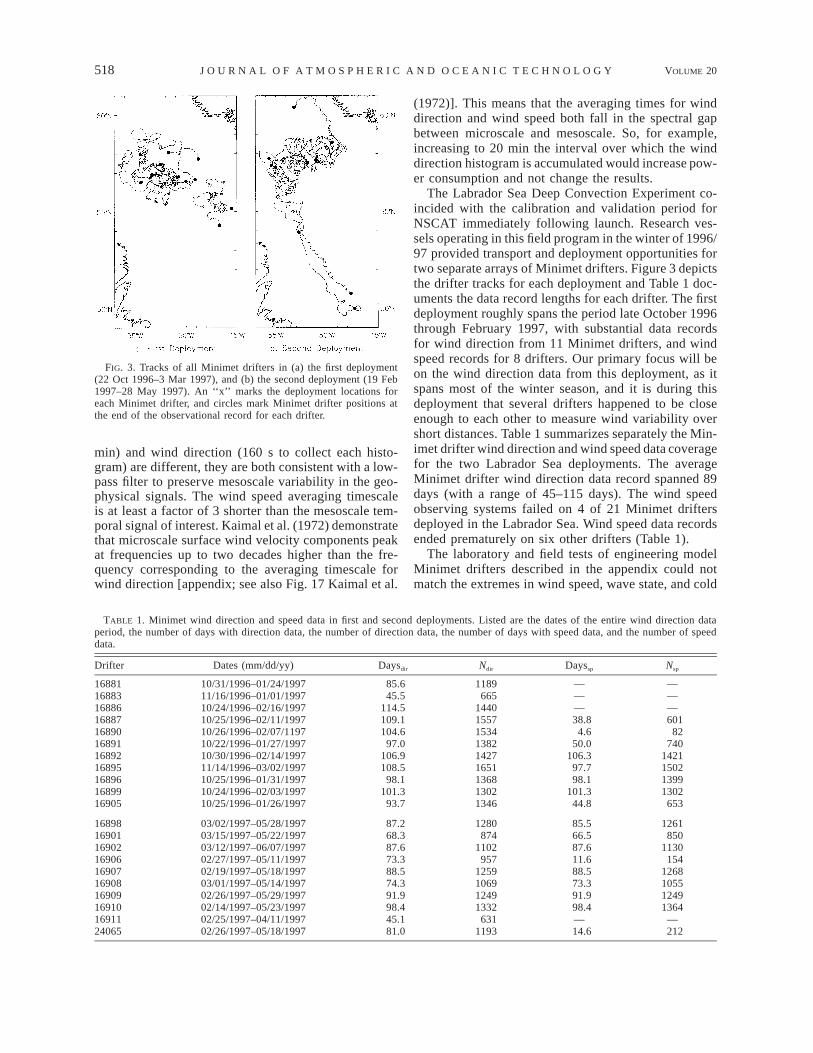
FIG. 3. Tracks of all Minimet drifters in (a) the first deployment(22 Oct 1996–3 Mar 1997), and (b) the second deployment (19 Feb1997–28 May 1997). An ‘‘x’’ marks the deployment locations foreach Minimet drifter, and circles mark Minimet drifter positions atthe end of the observational record for each drifter.

TABLE 1. Minimet wind direction and speed data in first and second deployments. Listed are the dates of the entire wind direction dataperiod, the number of days with direction data, the number of direction data, the number of days with speed data, and the number of speeddata.

Drifter Dates (mm/dd/yy) Daysdir Ndir Dayssp Nsp

1688116883168861688716890

10/31/1996–01/24/199711/16/1996–01/01/199710/24/1996–02/16/199710/25/1996–02/11/199710/26/1996–02/07/1197

85.645.5

114.5109.1104.6

1189665

144015571534

———38.8

4.6

———601

82168911689216895168961689916905

10/22/1996–01/27/199710/30/1996–02/14/199711/14/1996–03/02/199710/25/1996–01/31/199710/24/1996–02/03/199710/25/1996–01/26/1997

97.0106.9108.5

98.1101.3

93.7

138214271651136813021346

50.0106.3

97.798.1

101.344.8

7401421150213991302

653

1689816901169021690616907

03/02/1997–05/28/199703/15/1997–05/22/199703/12/1997–06/07/199702/27/1997–05/11/199702/19/1997–05/18/1997

87.268.387.673.388.5

1280874

1102957

1259

85.566.587.611.688.5

1261850

1130154

12681690816909169101691124065

03/01/1997–05/14/199702/26/1997–05/29/199702/14/1997–05/23/199702/25/1997–04/11/199702/26/1997–05/18/1997

74.391.998.445.181.0

106912491332

6311193

73.391.998.4—14.6

105512491364

—212

min) and wind direction (160 s to collect each histo-gram) are different, they are both consistent with a low-pass filter to preserve mesoscale variability in the geo-physical signals. The wind speed averaging timescaleis at least a factor of 3 shorter than the mesoscale tem-poral signal of interest. Kaimal et al. (1972) demonstratethat microscale surface wind velocity components peakat frequencies up to two decades higher than the fre-quency corresponding to the averaging timescale forwind direction [appendix; see also Fig. 17 Kaimal et al.

(1972)]. This means that the averaging times for winddirection and wind speed both fall in the spectral gapbetween microscale and mesoscale. So, for example,increasing to 20 min the interval over which the winddirection histogram is accumulated would increase pow-er consumption and not change the results.

The Labrador Sea Deep Convection Experiment co-incided with the calibration and validation period forNSCAT immediately following launch. Research ves-sels operating in this field program in the winter of 1996/97 provided transport and deployment opportunities fortwo separate arrays of Minimet drifters. Figure 3 depictsthe drifter tracks for each deployment and Table 1 doc-uments the data record lengths for each drifter. The firstdeployment roughly spans the period late October 1996through February 1997, with substantial data recordsfor wind direction from 11 Minimet drifters, and windspeed records for 8 drifters. Our primary focus will beon the wind direction data from this deployment, as itspans most of the winter season, and it is during thisdeployment that several drifters happened to be closeenough to each other to measure wind variability overshort distances. Table 1 summarizes separately the Min-imet drifter wind direction and wind speed data coveragefor the two Labrador Sea deployments. The averageMinimet drifter wind direction data record spanned 89days (with a range of 45–115 days). The wind speedobserving systems failed on 4 of 21 Minimet driftersdeployed in the Labrador Sea. Wind speed data recordsended prematurely on six other drifters (Table 1).

The laboratory and field tests of engineering modelMinimet drifters described in the appendix could notmatch the extremes in wind speed, wave state, and cold


FIG. 4. Sample wind direction calibration diagram for Minimetdrifter 16895. Wind direction difference (NSCAT 2 Minimet drifter)vs Minimet drifter wind direction is plotted for all collocations within60 min and 50 km. Collocation symbols correspond to refinementsin the collocation dataset used for Minimet calibration with NSCATas described in the text. A priori refinements are depicted accordingto separation distance (squares), wind speed regime (triangles), andpossible upwind/downwind ambiguity removal errors (diamonds).Numerals inside each symbol represent temporal separations in theNSCAT and Minimet collocations (multiply numerals by 10 min).The dashed line represents a uniform offset and the curve is the resultof a fit of sine and cosine terms derived independently for each drifter(and reported in Table 2).

temperatures that the Minimet drifters experienced inthe Labrador Sea. In addition to these calibrations, wedescribe in the next sections how collocated NSCATobservations in the Labrador Sea were used to removedistortions in Minimet wind direction observations andto standardize Minimet wind speed observations derivedfrom multiple WOTAN instruments. The collocation da-taset includes all Minimet drifter and NSCAT wind ob-servation pairs that occurred within 50 km and 60 minof each other. On average, there was one NSCAT col-location per day for each Minimet drifter. The LabradorSea experimental plan included the deployment of amoored meteorological instrument array that could alsohave been used to calibrate the Minimet drifters within situ data. Unfortunately, the moored system failedsoon after deployment.

a. Minimet wind direction calibration with NSCAT

As described in the appendix, the prototype Minimetdesign included features that later proved to be incom-patible in the creation of and sensitivity to local mag-netic fields. The flux gate compass component of thewind direction observation system was sensitive to mag-netic field effects from internal batteries and other mag-netized components within the drifter housing. Also, thecompass precalibrations to ameliorate the effects of in-ternal magnetic fields appear to have been distorted byan external magnet applied to each Minimet drifter upondeployment to initiate the observation duty cycles.

Laboratory tests of fully assembled Minimet driftersdemonstrated that the magnetic distortion was charac-terized by the superposition of a constant direction offsetand distortion sidelobe effects. We describe here a pro-cedure used to remove these distortions by fitting a cal-ibration curve to the distribution of the NSCAT minusMinimet wind direction difference versus the raw Min-imet wind direction. In order to apply the wind directioncorrection algorithm for the Minimet systems, a subset(Nfit) of the highest quality and most closely collocateddata was defined to conservatively exclude conditionswhen either the Minimet drifter or NSCAT might havebeen reporting erroneous, or low accuracy, measure-ments. As an example, we review the refinement of thecollocation dataset and calibration curve fit for Minimetdrifter 16895 as depicted in Fig. 4. Similar refinementsand wind direction calibrations were performed for eachMinimet drifter and a summary is provided in Table 2.

First, the collocation subset was limited to data thatwere within 20 km, so that the Minimet observationoriginated from a location within an NSCAT WVC. Fordrifter 16895, Fig. 4 indicates that most of the collocateddata are within this range. There are 21 data pairs withdistances greater than 20 km (the squares in Fig. 4). Ascatterplot of wind direction differences as a functionof time differences (not shown) indicates that the winddirection difference does not increase with time differ-ence for the range of spatial and temporal differences

considered here. This is also apparent in Fig. 4, wherethe time differences for each collocation symbol areindicated by numerals to be multiplied by 10 min withineach symbol. All collocations within 60 min of eachother were included in Nfit. The calibrations were notfound to be significantly changed if the collocationswere restricted to time differences # 30 min.

Second, Nfit was refined according to reliable windspeed ranges. On a global basis, the NSCAT wind re-trievals are deemed most accurate for wind speeds of3–30 m s21 (NASA Scatterometer Project 1998). Winddirection observations are always problematic ap-proaching the limit of zero wind speed where directionis undefined. Predeployment tests of engineering modelMinimet drifters reported in the appendix (see Fig. 11)found that wind direction estimates were in better agree-ment with each other for wind speeds in the range 6–7 m s21, than for speeds of 2–3 m s21. At lower windspeeds, the wind direction observation by Minimet wasmore sensitive to contamination by swell effects. Thescatterplot of all Minimet versus NSCAT wind directiondifferences as a function of wind speed (not shown here)demonstrates a few anomalously high differences be-tween Minimet and NSCAT data at small wind speeds,but no other dependence on speed. So a minimum speedof 5 m s21 is used to further limit the Nfit collocations.For drifter 16895 this resulted in six data being excludedfrom Nfit, as indicated by the triangles in Fig. 4.

Third, when the wind direction difference betweendrifter and NSCAT exceeded 908, data were not used.The few large direction differences were assumed to be


TABLE 2. Minimet calibration coefficients for wind direction and speed. Listed are the number of collocated drifter and NSCAT data foreach drifter, the number of collocated data used to fit the calibration function, the mean distance and the mean time difference of collocateddata, and the resulting calibration coefficients. The wind speed calibration coefficients are based on the 1–2-kHz band.

Drifter Nco–loc

Wind direction

Nfit

DX(km)

DT(min) C0 C1 C2 C3 C4

Wind speed

Nfit S I

1688116883168861688716890

734396

105105

6025687076

1011101010

2520222323

24.220.322.214.7

24.8

6.2228.5

0.72.5

12.4

5.66.11.8

10.328.6

28.44.2

18.0223.5

4.7

24.2213.0

0.126.9

213.8

———39

6

———

0.0620.067

———

2.0691.592

168911689216895168961689916905

8391

112858482

576484616262

111110101111

222320212721

23.012.2

9.70.89.4

20.9

21.69.29.4

20.624.5

214.5

23.623.1

6.53.0

20.4225.1

4.51.2

11.428.824.928.8

26.021.723.526.2

210.1211.1

388897838138

0.0630.0720.0660.0640.0610.060

2.2232.7432.3641.8812.4112.356

1689816901169021690616907

8753616989

5236394555

1011101010

2423222124

233.840.2

20.1210.7

6.6

228.226.613.8

6.510.8

214.721.2

4.420.9

8.0

5.5213.1

2.18.86.7

23.927.724.123.6

211.4

8150611385

0.0740.0530.0630.0490.065

1.5312.8672.6154.5632.696

1690816909169101691124065

7580893679

4656673053

910111011

2222282522

55.5214.8

9.7245.024.4

5.317.810.110.8

22.3

12.73.7

25.32.7

215.9

4.0212.6

10.9221.2

24.3

15.8210.228.3

222.7218.5

717790—13

0.0630.0620.063

—0.068

2.4585.0352.346

—2.026

Avg 80 56 10 23 59

due to erroneous NSCAT data suffering from an incor-rect upwind/downwind ambiguity removal (e.g., seeGonzalez and Long 1999).

After these three a priori refinements on Nfit, the av-erage direction difference and the standard deviation ofthe differences were computed. In a final refinement ofNfit before curve fitting, all collocated pairs for whichthe direction differences exceeded 2 standard deviationswere eliminated. The remaining Nfit collocations (circlesin Fig. 4) are used to determine five calibration coef-ficients in the function:

dir 2 dirNSCAT Minimet

5 C 1 C sin(dir ) 1 C sin(2 3 dir )0 1 Minimet 2 Minimet

1 C cos(dir ) 1 C cos(2 3 dir ).3 Minimet 4 Minimet

This procedure was repeated for each drifter indepen-dently. The Nfit and coefficients Cn, where n 5 0, 1, 2,3, 4, are listed for the entire Minimet dataset in Table 2.

For drifter 16895, we began with 112 collocated datapairs, and used 84 pairs for calibration. For this subset,the average distance between drifter and NSCAT datawas 10 km, and the average time difference betweenobservations was 20 min. The resulting calibration func-tion for drifter 16895 is shown in Fig. 4.

Over all Minimet drifters, the offset coefficients C0,ranged between 245.08 and 155.58. There is no con-sistent pattern in the variations for any of the Cn whencompared drifter to drifter. Subsequently, we havelearned that small changes in the internal placement

relative to the compass of the potentially magnetizedcomponents, especially the battery pack, make a bigdifference in the relative magnetization of the fully as-sembled float. The magnetic activation switch was re-placed by a mechanical switch in later Minimet designs.

b. Minimet wind speed calibration with NSCAT

The WOTAN technology of inferring near-surfacewind speed from underwater acoustic noise is thor-oughly discussed in Vagle et al. (1990). The relation-ships are empirical and have typically been either log-arithmic or linear, where the noise is a broadband rmspressure. Here we use a different broadband measure,PMinimet, that is the accumulations of from 50 to 100narrowband measurements of rms acoutic pressure. Thisprocedure is detailed in the appendix.

NSCAT wind speed is linearly regressed againstPMinimet (see appendix), in each of the eight broad fre-quency bands to determine the slope (S) and intercept( I) of the calibration (Table 2):

speed 5 SP 1 I.NSCAT Minimet

Points that were more than 2 standard deviations offthis initial fit were discarded and the linear fit was per-formed again. Those individual fits vary from drifter todrifter by 20% in slope, which may be indicative of thedifferent hydrophone sensitivities and power amplifi-cation. Positive intercepts were attributed by Vagle etal. (1990) to a wind threshold required to drive the


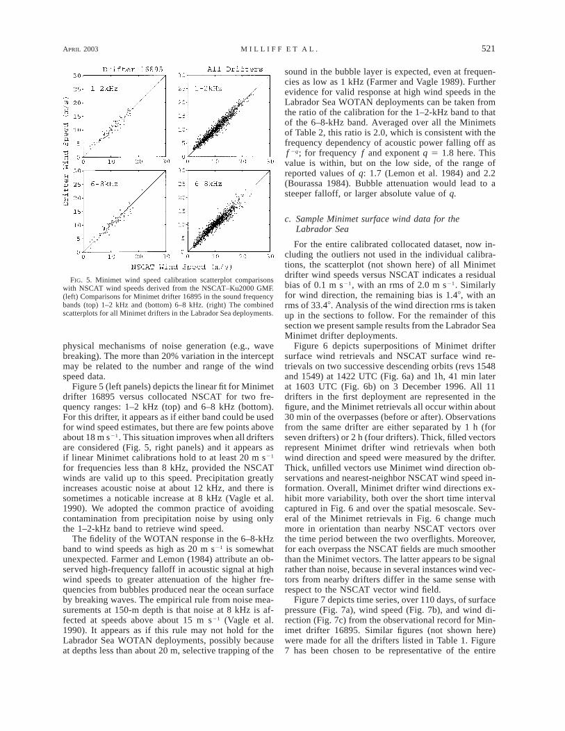
FIG. 5. Minimet wind speed calibration scatterplot comparisonswith NSCAT wind speeds derived from the NSCAT–Ku2000 GMF.(left) Comparisons for Minimet drifter 16895 in the sound frequencybands (top) 1–2 kHz and (bottom) 6–8 kHz. (right) The combinedscatterplots for all Minimet drifters in the Labrador Sea deployments.

physical mechanisms of noise generation (e.g., wavebreaking). The more than 20% variation in the interceptmay be related to the number and range of the windspeed data.

Figure 5 (left panels) depicts the linear fit for Minimetdrifter 16895 versus collocated NSCAT for two fre-quency ranges: 1–2 kHz (top) and 6–8 kHz (bottom).For this drifter, it appears as if either band could be usedfor wind speed estimates, but there are few points aboveabout 18 m s21. This situation improves when all driftersare considered (Fig. 5, right panels) and it appears asif linear Minimet calibrations hold to at least 20 m s21

for frequencies less than 8 kHz, provided the NSCATwinds are valid up to this speed. Precipitation greatlyincreases acoustic noise at about 12 kHz, and there issometimes a noticable increase at 8 kHz (Vagle et al.1990). We adopted the common practice of avoidingcontamination from precipitation noise by using onlythe 1–2-kHz band to retrieve wind speed.

The fidelity of the WOTAN response in the 6–8-kHzband to wind speeds as high as 20 m s21 is somewhatunexpected. Farmer and Lemon (1984) attribute an ob-served high-frequency falloff in acoustic signal at highwind speeds to greater attenuation of the higher fre-quencies from bubbles produced near the ocean surfaceby breaking waves. The empirical rule from noise mea-surements at 150-m depth is that noise at 8 kHz is af-fected at speeds above about 15 m s21 (Vagle et al.1990). It appears as if this rule may not hold for theLabrador Sea WOTAN deployments, possibly becauseat depths less than about 20 m, selective trapping of the

sound in the bubble layer is expected, even at frequen-cies as low as 1 kHz (Farmer and Vagle 1989). Furtherevidence for valid response at high wind speeds in theLabrador Sea WOTAN deployments can be taken fromthe ratio of the calibration for the 1–2-kHz band to thatof the 6–8-kHz band. Averaged over all the Minimetsof Table 2, this ratio is 2.0, which is consistent with thefrequency dependency of acoustic power falling off asf 2q; for frequency f and exponent q 5 1.8 here. Thisvalue is within, but on the low side, of the range ofreported values of q: 1.7 (Lemon et al. 1984) and 2.2(Bourassa 1984). Bubble attenuation would lead to asteeper falloff, or larger absolute value of q.

c. Sample Minimet surface wind data for theLabrador Sea

For the entire calibrated collocated dataset, now in-cluding the outliers not used in the individual calibra-tions, the scatterplot (not shown here) of all Minimetdrifter wind speeds versus NSCAT indicates a residualbias of 0.1 m s21, with an rms of 2.0 m s21. Similarlyfor wind direction, the remaining bias is 1.48, with anrms of 33.48. Analysis of the wind direction rms is takenup in the sections to follow. For the remainder of thissection we present sample results from the Labrador SeaMinimet drifter deployments.

Figure 6 depicts superpositions of Minimet driftersurface wind retrievals and NSCAT surface wind re-trievals on two successive descending orbits (revs 1548and 1549) at 1422 UTC (Fig. 6a) and 1h, 41 min laterat 1603 UTC (Fig. 6b) on 3 December 1996. All 11drifters in the first deployment are represented in thefigure, and the Minimet retrievals all occur within about30 min of the overpasses (before or after). Observationsfrom the same drifter are either separated by 1 h (forseven drifters) or 2 h (four drifters). Thick, filled vectorsrepresent Minimet drifter wind retrievals when bothwind direction and speed were measured by the drifter.Thick, unfilled vectors use Minimet wind direction ob-servations and nearest-neighbor NSCAT wind speed in-formation. Overall, Minimet drifter wind directions ex-hibit more variability, both over the short time intervalcaptured in Fig. 6 and over the spatial mesoscale. Sev-eral of the Minimet retrievals in Fig. 6 change muchmore in orientation than nearby NSCAT vectors overthe time period between the two overflights. Moreover,for each overpass the NSCAT fields are much smootherthan the Minimet vectors. The latter appears to be signalrather than noise, because in several instances wind vec-tors from nearby drifters differ in the same sense withrespect to the NSCAT vector wind field.

Figure 7 depicts time series, over 110 days, of surfacepressure (Fig. 7a), wind speed (Fig. 7b), and wind di-rection (Fig. 7c) from the observational record for Min-imet drifter 16895. Similar figures (not shown here)were made for all the drifters listed in Table 1. Figure7 has been chosen to be representative of the entire


FIG. 6. Surface vector wind retrievals from consecutive NSCAT descending orbits and coincident Minimet drifters in the Labrador Seaon 3 Dec 1996 (a) at 1422 UTC for rev 1548, and (b) at 1603 UTC for rev 1549. In both panels the satellite moves from north to south.During rev 1548 the 600-km-wide right side of the swath (24 across-track WVC) covers most of the Labrador Sea. In the next revolutionthe left half of the swath overlaps with the previous swath. All 11 Minimets of the first Labrador Sea deployment are depicted in each panel.The Minimet observations all occurred within 37 min (before or after) of the first overpass, and again within 32 min of the second overpass.Filled vectors are data with drifter observed wind direction and speed, and unfilled vectors are observed drifter direction but nearest-neighborNSCAT speed.

dataset. Open circles in the middle and bottom panelsare the superposition of collocated NSCAT wind speedand wind direction retrievals, respectively.

Large-amplitude wind speed events in Fig. 7 oftencoincide with local surface pressure minima and abruptchanges in wind direction. These coincident changes areconsistent with the development and propagation of syn-optic-scale systems such as shown in Fig. 1. In fact,wind speed and direction observations for drifter 16895account for the northernmost Minimet drifter vector inFig. 1. The pressure and wind direction changes thatcorrespond to the local wind speed maximum for thesynoptic setting in Fig. 1 are evident around day 397in Figs. 7a and 7c.

Note, however, that for a few large wind speed events(e.g., around days 393 and 409) the NSCAT retrievalssubstantially exceed the Minimet maxima with speedestimates greater than 30 m s21. Similarly, a few large-amplitude wind speed events in the Minimet record(e.g., around days 346 and 367) are not sampled byNSCAT. The Minimet wind speed estimate on day 367is as large as 30 m s21. For the entire dataset, there arenot sufficient numbers of coincident Minimet andNSCAT observations for wind speeds in excess of 25

m s21 to either validate NSCAT retrievals with Minimet,or conversely, to conclude that Minimet wind speedsensitivity is saturating, at very high wind speeds. Thereare instances of coincident observations for wind speedsin excess of 20 m s21 in Fig. 7 (e.g., around days 345and 385); and as previously noted, Fig. 5 indicates thatother drifter records contain coincident observations inthe 20–25 m s21 range as well.

The wind direction time history (Fig. 7c) is of par-ticular interest. The efficacy of the wind direction cal-ibration with NSCAT is demonstrated by instances ofO(1008) direction changes tracked by both instrumentsystems over intervals as short as the time span of suc-cessive overflights (e.g., day 380). Superposed on thedirection variability that occurs on the order of days thatis well represented in both NSCAT and Minimet records,there exists a much shorter timescale variability appar-ent in only the Minimet record. The amplitude of thishigher frequency variability is O(408) and it occursthroughout the record in Fig. 7c, and is typical of winddirection time histories for all the Minimet drifters inthe Labrador Sea deployments. This variability is alsoconsistent with the visual distinctions between NSCATand Minimet in Fig. 6. It is much larger in amplitude


FIG. 7. Time series for drifter 16895 of (a) air pressure, (b) wind speed, and (c) wind direction for 110 days spanning much of the firstLabrador Sea deployment. Open circles in wind speed and direction time series are for collocated NSCAT data as derived from the Ku2000GMF.

than the uncertainty estimates (i.e., 68–88) for Minimetwind direction observations derived from the prelimi-nary field calibrations described in the appendix.

4. Discussion

In this section, we take up the issues involved incomparing the Minimet and NSCAT datasets, which arenot independent because of the Labrador Sea field cal-ibrations for each Minimet drifter. It remains for us toquantify the visual inferences from Figs. 6 and 7 ofshorter time- and space scale variability in the surfacewind field that we associate with an energetic mesoscale.We argue this case in two ways. First, in differencingvector wind observations from Minimet drifters over awide variety of synoptic conditions and spatial scalesto reduce the amplitude of large-scale signals, and sec-ond by comparing records for Minimet drifter groupsthat were very near each other for periods of many days,under relatively constant large-scale wind conditions.

a. Rms differences versus spatial separation

Observations of the surface wind speed and directionvariabilities as a function of spatial scale are representedas rms differences versus separation distance in Fig. 8.Each drifter record was compared against the recordsfrom all other drifters. Whenever observations from twodifferent drifters occurred within 30 min of each other,the differences in wind speed and direction were as-signed to the spatial separation bin corresponding to theseparation distance at the time of the observations (binsdiscretized into 20-km intervals from 0 to 400 km). Inorder to concentrate on the winter season, the period ofinterest was restricted to November 1996 through March1997.

The region of the Labrador Sea over which the speedand direction differences from NSCAT were accumu-lated was limited to match the subdomain occupied bythe Minimet drifters (i.e., the central basin; see Fig. 3a).Even so, spatial coverage within the NSCAT swath is


FIG. 8. Rms differences vs spatial separation for (a) wind speed and (b) wind direction from coincidentfields of Minimet (filled circles) and NSCAT (open circles) observations. An estimate of the uncertainty(ranges indicated by vertical lines, and 1 std dev indicated by boxes) of the rms differences is provided asdescribed in the text. (c) The number of differences (i.e., bin counts) for each spatial separation bin, forNSCAT (open circles, both speed and direction), Minimet wind directions (filled circles), and wind speeds(filled circles with x’s).

dense and many more speed and direction differencesare possible for spatial separations within the swath di-mension. To balance the numbers of NSCAT and Min-imet differences per spatial separation bin, NSCAT dif-ferences were randomly selected from the swath obser-

vations until the number of differences roughly matchedthe number of Minimet direction differences in eachspatial separation bin (ca. 2600). The NSCAT rms val-ues are found to be insensitive to increase of samplesize by factors of 10 or even 100.


The Minimet and NSCAT bin counts used in Figs.8a and 8b are shown in Fig. 8c. There are about 4 timesas many Minimet wind direction difference pairs thanthere are Minimet wind speed difference pairs. For spa-tial separations between 0 and 20 km, only Minimetdifferences were possible, and there were 332 windspeed differences and 1242 wind direction differencesfor this bin. We selected more evenly distributed bincounts for the NSCAT differences in both speed anddirection (Fig. 8c).

No account has been made of spatial and/or temporaldependence in the observations that comprise the dif-ferences from either observing system. This is not acrucial approximation in that while differences will notbe independent for the same two drifters whose sepa-ration distances are within the same spatial separationbin over several hours, the bin counts attest to the factthat there are many such episodes for many differentdrifter pairs in the summaries presented in Fig. 8. Con-versely, for the NSCAT differences, it is probable thatdifferences over a wide range of spatial separation binsall taken from the same swath might not be independent(i.e., if the differences are reflective of the same syn-optic-scale event). However, with O(1000) differencesin each bin, drawn uniformly from an observing periodthat spans more than 150 days and about 190 differentsatellite swaths, we are confident that no single synopticevent dominates the analysis. To be sure, we analyzeda subset of the drifter and NSCAT differences restrictedto include only the difference pairs when both Minimetand nearby NSCAT wind estimates were available atthe same times. While this limits the bin counts in manyspatial separation bins to fewer than 100, the results tobe described below are not significantly changed.

A bootstrap method for estimating the 1 standard de-viation spread of the rms differences in speed and di-rection is depicted in Figs. 8a and 8b, respectively. Toestimate the standard deviation in rms difference foreach spatial separation bin the following procedure wasimplemented. The rms difference is recomputed 50times from randomly drawn subsamples of the total pop-ulations of wind direction or wind speed differences ineach bin. The subsample population sizes are set equalto one-half the respective bin counts. Boxes indicating1 standard deviation in the rms difference are drawn foreach circle (filled and open) in Figs. 8a and 8b. Verticalbars indicate the ranges of the rms difference estimatesfrom the 50 subsamples in each bin. While the rangesvary somewhat depending upon the number of subsam-ples and/or the size of each subsample, the estimatesfor 1 standard deviation are more stable.

Figure 8a shows the rms difference for speed versusspatial separation; filled circles with ‘‘x’s’’ represent theMinimet results for each spatial bin, and open circlesrepresent NSCAT. Both datasets exhibit a linear increasein wind speed difference as a function of spatial sepa-ration out to at least 200-km separations (wind speedrms ; 4.5 m s21). The NSCAT differences continue in

a linear trend of shallower slope to 400 km (NSCATwind speed rms ; 6.0 m s21), while the Minimet drifterwind speed rms is widely scattered between 3 and 6 ms21 for bins between 200 and 400 km. Both datasets aresuggestive of an intercept of the y axis at about windspeed rms ; 1.0 m s21. These intercepts are within theglobal wind speed accuracy specifications for theNSCAT mission (NASA Scatterometer Project 1998).

We should also recognize that these rms interceptsare our best estimates of the combined instrument noise(different for each observing system) and natural var-iability of the surface wind speed in the Labrador Sea,in winter, at spatial scales too short to be well resolvedby either observing system. This estimate of spatial-scale variability can be considered in light of short tem-poral-scale variability of the mesoscale surface windfield from Austin and Pierson (1999). In that study, theauthors filtered time series of mesoscale observationsfrom moored buoys in the North Atlantic and Gulf ofMexico, and compared the filtered and unfiltered dataon scatterplots. Austin and Pierson (1999) found rmsdifferences on the order of 1 m s21 between the filteredand unfiltered datasets.

If we adopt for the case of mesoscale surface winds,a Taylor hypothesis as introduced for the microscalewinds earlier, we can assume an equivalence betweenmesoscale temporal and mesoscale spatial fluctuationsof the surface wind speed. In that case, the rms interceptsin Fig. 8a and the results of Austin and Pierson (1999)are roughly consistent. We note, however, assuming aTaylor hypothesis construct for the mesoscale surfacewind field is very much an open question.

Figure 8a also demonstrates that the wind speed rmsdifferences at short spatial separations are not useful todistinguish the sensitivities of Minimet or NSCAT sys-tems to the mesoscale surface wind signal.

Figure 8b depicts the average rms differences in sur-face wind direction as a function of spatial separationdistance; filled circles for the Minimet drifters, and opencircles for randomly sampled NSCAT differences. Therms wind direction differences are significantly largerfor Minimet comparisons than for NSCAT comparisonsat all spatial separations. Moreover, the distinction inrms wind direction differences between the two ob-serving systems is roughly constant at about 208 overa large range of spatial separations; for example, from20 to almost 700 km (not shown). For the shortest spatialseparations (20–40 km), the rms direction differencefor NSCAT pairs is around 108, while it is around 358for Minimet comparisons. At 400 km, the average rmsdirection difference for NSCAT is about 458, and forMinimet drifters, about 658.

As in the case of the wind speed differences, in ad-dition to the true mesoscale wind direction variabilitysignal, these rms differences also contain a part due tonoise in the observing systems. In the Minimet case,estimates of a noise term on the order of about 88 comefrom field tests off California with engineering model


FIG. 9. Data record comparisons for nearby Minimet drifters 16896and 16886. Panels depict time series for (a) separation distance, (b)wind speed from Minimet 16896 (no data from 16886), (c) winddirection (16896 filled circles, and 16886 open circles), and (d) winddirection difference over more than 4 days. (c) Smooth solid (for16896) and dashed (for 16886) lines depict 12-h running mean winddirection time series. (d) The wind direction differences are computedafter removing the respective 12-h running means.

TABLE 3. Rms wind direction differences of nearby drifters during steady wind conditions. For each drifter pair the average distance, theaverage time difference, the average speed, the number of data, and the rms wind direction are listed. There are five separate events. Thedirection differences are based on drifter directions that are adjusted by the half-day running mean of each drifter (see Fig. 9d).

Drifter, pair Days Period (days) DX (km) DT (min) Speed (m s21) Nrms Dirrms

16905, 1689916905, 1688716905, 1688616899, 1688716899, 1688616887, 16886

302.7–304.5302.7–304.5302.7–304.5302.7–304.5302.7–304.5302.7–304.5

1.81.81.81.81.81.8

2.49.42.8

10.11.09.7

252920102924

7.67.67.57.77.87.7

232624222324

31.337.429.936.129.919.2

16905, 1689916905, 16887

310.5–312.0310.5–312.0

1.51.5

9.510.1

2529

10.210.4

2324

16.319.6

16886, 1689616891, 1689616905, 16890

340.5–344.0342.8–344.1347.8–350.4

3.51.32.6

8.49.35.0

83329

12.610.0—

461333

28.112.112.1

16891, 1688616891, 1688616891, 16886

348.3–350.6351.5–352.4353.2–354.6

2.30.91.4

9.37.99.2

161315

———

321324

18.329.322.1

16891, 1689916891, 1689916891, 16899

371.6–376.0376.4–380.0382.7–385.4

4.43.62.7

2.43.05.0

202023

16.87.7

19.9

604724

16.528.515.9

Total/avg 36.5/2.1 7.0 22 11.6 481/28 24.6

Minimet drifters (appendix). To be careful, we let theMinimet wind direction observing system noise estimatein the Labrador Sea case be O(108) to account for anyresidual errors after the calibration with NSCAT direc-tions.

b. Minimet records for drifters in close proximity

To further explore the signal-to-noise budget for theLabrador Sea Minimet wind direction observations, wecompare records for Minimets that were very near eachother in space (,12 km) and time (,30 min) duringrelatively constant wind events (speeds and directions)that occurred for longer than a day. A sample compar-ison of nearby Minimet drifter wind direction estimatesis shown in Fig. 9. Minimet drifters 16886 and 16896were within 10 km of each other for 3.5 days. The winddirection time series for each Minimet drifter are de-picted in Fig. 9c. A half-day running mean directiontrace is also shown for each drifter, and these demon-strate that the drifters are measuring the same synoptic-scale wind directions. In addition, there is a short time-scale variability in wind direction that differs betweendrifters even over this very short separation distance(average separation over the period is 8.4 km). The di-rection differences for the case shown in Fig. 9 arecomputed after removing the respective running meandirections. The time series of the differences is shownin Fig. 9d. The rms direction difference is 28.18 for thisparticular episode and drifter pair (see Table 3).

Five separate episodes, involving seven differentdrifters in 18 pairings, are summarized in Table 3. Alsolisted in the table are the rms differences in wind di-rection observations during these periods. The average


rms wind direction difference over 481 Minimet drifterpairs is 258. Again, we have not accounted for temporaland spatial dependence in the sequences of paired ob-servations used in this calculation, but rely instead uponthe abundance of observations and the diversity ofevents to average the effects of these dependencies. Ineach of the cases examined, the 0.5-day running meandirections are very similar for the drifter pairs.

The proximity of the Minimet drifter pairs examinedin Table 3 limits the feasible spatial scales for variabilityin the surface wind field. As such, the rms directiondifferences probably provide a lower bound on the partof the rms direction difference due to true mesoscalefluctuations in the surface wind field. Given our estimateof Minimet wind direction observing system instrumentnoise (108), and the signal-plus-noise estimate from Ta-ble 3 (258), an estimate of the mesoscale direction var-iability signal detected by the Minimet drifters in theLabrador Sea is about 238 (i.e., 232 ø 252 2 102).Again, given a Taylor hypothesis for mesoscale windfluctuations on these scales, this estimate compares wellwith independent estimates of the mesoscale surfacewind variability in the North Atlantic and Gulf of Mex-ico due to Austin and Pierson (1999). Their estimatesfor the standard deviation of wind direction based ontemporal variability in moored buoy observations at 10-m height is 19.78.

Figure 8b shows that the wind direction differencesdetected by NSCAT are much lower than Minimet es-timates over all spatial separations. We relate this to thecombined effects of compositing radar backscatter sig-nals within each WVC, and the median filter methodused to select among wind direction ambiguities thatarise from the NSCAT–Ku2000 model function inver-sion. While the details of the median filter are beyondthe scope of this paper, comparisons with coarse-reso-lution weather center analyses at the initial iteration,and comparisons with neighboring WVC directions insubsequent iterations of the median filter, are operationsthat smooth out spatial variability within the NSCATswath. This removes a mesoscale signal in wind direc-tion that is detectable in the Minimet observations[O(238) rms].

The median filter and/or GMF inversions do not ap-pear to affect in a similar way the NSCAT wind speeddifferences for short spatial separations. However, as wehave noted, the rms of wind speed differences over shortspatial separations is affected by the expected windspeed accuracy limits for NSCAT. As we have also not-ed, the ambiguous vectors that emerge from the GMFinversions typically do not vary in wind speed as muchas wind direction. The median filter operation thenserves to distinguish wind directions but not windspeeds among the ambiguities. It is consistent with therms differences in Figs. 8a and 8b to suspect that me-soscale spatial variability in NSCAT wind speeds is notfiltered, but it is filtered in wind direction.

c. Spatial correlation model estimates

The Minimet detection of the mesoscale wind fieldin the Labrador Sea can be extended to obtain estimatesof the characteristic length scales for surface wind me-soscale variability for the winter of 1996/97. As in thecase for wind speed and direction in Fig. 8, we cancompare the rms differences in eastward (u) and north-ward (y) velocity components as functions of spatialseparation. Separate spatial correlation models can thenbe fit for u and y, and correlation length scales estimatedbased on those fits. We revert to estimates based onvelocity components because, unlike wind direction, uand y are scalar fields where possible amplitude differ-ences are unbounded. This is important in the correlationfunction derivation described below. Moreover, con-structing velocity component estimates from Minimetobservations is consistent given that mesoscale vari-ability has been preserved in both wind speed and di-rection retrievals.

To remove the large-scale climatological differencesin u and y, the NSCAT wind vectors were averaged into18 lat 3 18 lon bins for the winter dataset in the LabradorSea. Using the Minimet position information, we haveremoved the appropriate 18 winter-average u and y com-ponents from the Minimet components before comput-ing the rms differences versus spatial separation.

In the following, we demonstrate the derivation of aspatial correlation model for an arbitrary spatially de-pendent scalar function, f(Dx), where Dx 5 xi 2 xj. Therms difference in pairs of observations of f is given by

1/2N2112f (Dx) 5 [ f (x) 2 f (x 1 Dx)] . (1)Orms 5 6N j51

Using this, form a quantity f * as

12f * 5 [ f ] . (2)rms2

Then the expected value of f * is

12E [ f *] 5 {E [ f (x ) ] 2 2E [ f (x )]E [ f (x )]i i j2

21 E [ f (x ) ]}j

25 s 2 cov[ f (x ), f (x )]i j

25 s {1 2 corr[ f (x ), f (x )]}, (3)i j

where E[ · ] is the expectation operator, s2 is the fieldvariance, cov[ f (xi), f (xj)] is the spatial covariance func-tion, and corr[ f (xi), f (xj)] is the spatial correlation func-tion for f (x). Assuming the general class of exponentialspatial covariance models, we have

2DxE [ f *] 5 a 2 b exp . (4)[ ]u

In the spatial statistics literature (e.g., Isaaks and Sri-vastava 1989), a is called the sill that corresponds to


FIG. 10. Spatial correlation model fits for (a) zonal and (b) merid-ional wind component terms (e.g., u* and y* terms as described inthe text). Plus signs indicate the scatter in each component as afunction of spatial separation bin, and the curve is described by thespatial correlation model (4) in the text. Parameters and their std devfor the spatial correlation model are listed in each panel.

the field variance s2, and a 2 b is called the nugget,which is related to measurement uncertainty. The pa-rameter u is called the range and it is the e-folding scalefor the exponential model for E[ f *]. The exponentialmodel is fit such that at large Dx . u, E[ f *] goes tothe field variance; and at very small Dx, E[ f *] goes tothe nugget.

Figure 10 demonstrates the u* (Fig. 10a) and y* (Fig.10b) versus spatial separation for the Minimet observa-tions, and the corresponding exponential correlation mod-el fits. Velocity component analyses require Minimetmeasurements of both wind speed and direction. Thislimits the bin counts for each spatial separation bin to

the lower bin counts for wind speed described in Fig. 8c.However, the model fits are sensible and the model pa-rameter estimates and uncertainties are listed in Fig. 10.

The correlation model fits are best for spatial sepa-rations from 0 to 400 km for both velocity components.Visual inspection of Fig. 10 indicates that the fit in yis better over that range than is the fit for u. Parameteruncertainties listed in Fig. 10 indicate that the fit in yis tighter over the entire range. The characteristic lengthscales (from estimates of u) are about 290 km in thezonal direction and 250 km in the meridional direction.These scales are well within the range of the spatialscales over which rms differences were collected, andwell spanned by the region of the Labrador Sea occupiedby the drifters during the winter season.

The nugget values for u* and y* can be manipulatedto compare with rms wind speed and wind directiondifferences at 0 separation in Figs. 8a and 8b. The nug-get from the correlation model for u* is about 5.5 m2

s22, and the nugget for y* is about 7.5 m2 s22. If wedouble these and take square roots, we obtain units ofrms, or 3.3 and 3.8 m s21, for u and y, respectively.These amplitudes are more than 3 times larger than therms at 0 separation for wind speed differences in theMinimet drifter dataset. From what we have seen of thedirection variability (e.g., Fig. 7), we can attribute mostof the implied component amplitudes at 0 separation tothe effects of wind direction variability.

The correlation model (4) is specific to spatial vari-ability only. As such, the mesoscale surface wind lengthscale estimates do not account for temporal effects andthe organization of coherent mesoscale structures in thewind field as described for Fig. 1. To account simul-taneously for space–time variability is much more chal-lenging, and even the combined Minimet and NSCATdatasets are not likely to be sufficient given standardmethods. Common practice then resorts to methods ofdata assimilation wherein reinitializations and integra-tions of a numerical forecast model are required to con-strain the field estimation problem. Alternatively, newapproaches employing Bayesian hierarchical models areunder development (Royle et al. 1999; Wikle et al. 1998;Wikle et al. 2001; Berliner et al. 2003).

5. Summary

Coincident estimates of the surface wind field in theLabrador Sea were retrieved from NSCAT observationsand two deployments of Minimet drifters over the periodOctober 1996–May 1997. The Minimet drifter repre-sents a new technology for in situ observations of thesurface wind field from ocean current following plat-forms in remote, and often harsh, environments. Min-imet wind speeds are inferred from ambient acousticnoise (WOTAN), and a vane fixed to the surface floatis used to infer wind direction.

Minimet drifter development and predeployment cal-ibrations are reviewed in the appendix. The effective


temporal averaging of acoustic pressure signals, and thetime interval over which a wind direction histogram isaccumulated are shown to be consistent with low-passfiltering of microscale wind variabilities, and the pres-ervation of the mesoscale.

Minimet drifters are designed to be inexpensive andpower efficient so that many drifters can be deployedat a time to operate for a season or more. The Minimetdrifter wind speed and direction observations have beencalibrated with NSCAT. The relative calibration of drift-ing in situ systems with comparable observations froma spaceborne remote sensing system demonstrates a util-ity of the so-called modern ocean observing system(e.g., Smith and Koblinsky 2001). Such calibrations arecarried out for the full field lifetime of the in situ sys-tems, and therefore can involve many comparative mea-surements. Several deployments, in many differentocean basins, might one day be cross-calibrated in thisway over the lifetime of the spaceborne observing sys-tem.

In the Labrador Sea case, a high-frequency O (hourly),large-amplitude O(408) variability in wind direction isevident in all Minimet time series after calibration withNSCAT (e.g., Fig. 7). An approximate signal-to-noisebudget is possible given predeployment calibration dataand multiple instances of multiday records from nearbydrifter groupings in the Labrador Sea. Minimet winddirection instrument noise is probably less than 108.Mesoscale surface wind direction temporal variabilityoccurs on hourly timescales, and with typical amplitudesaround 238.

Variability of this kind is consistent with estimatesfor mesoscale wind variability from independent anal-yses based on single-point moorings in other ocean re-gions (Austin and Pierson 1999). This consistency de-pends upon a heretofore unsubstantiated assumption thatmesoscale temporal and spatial variability are equivalentin the sense of a Taylor hypothesis. We note that severalfield campaigns, involving multiple Minimet deploy-ments in a variety of surface wind regimes, could beused to test such an assumption for mesoscale surfacewind variability.

A spatial correlation model fit to rms wind directiondifferences versus spatial separation yields estimates ofthe spatial scale of variability in the surface mesoscalewind for the Labrador Sea in winter. The estimatedlength scales are 290 km in the zonal direction and 250km in the meridional direction. Estimates for the me-ridional length scale are less noisy than for the zonalscale. These estimates do not account for mesoscaletemporal variabilities that are not well enough resolvedin the combined Minimet and NSCAT datasets for usein conventional space–time models. Nonetheless, theselength scales are consistent with the dimensions of co-herent mesoscale regimes identified in different sectorsof a polar low synoptic circulation system (Fig. 1).

To the extent that the Minimet wind speed observa-tions have been standardized in the Labrador Sea de-

ployments, there is validation information available withrespect to NSCAT. The calibration of Minimet responsein the 1–2 kHz band for wind speeds in the 20–25 ms21 range of the Labrador Sea observations does notdiffer from calibrations for lower wind speed ranges(Figs. 5 and 7). This implies a consistency and validityin the NSCAT retrievals at these higher wind speedswhere validation data are difficult to obtain. In terms oflimitations of the NSCAT dataset, we have demonstratedthat a mesoscale variability in surface wind direction issmoothed out of the NSCAT retrievals, possibly in thecompositing of multiple backscatter returns over eachWVC, and/or in the median filter step of the NSCATprocessing used to resolve directional ambiguities. Fi-nally, even in the case of the unprecedented abundanceof surface wind field data for the Labrador Sea fromNSCAT, the Minimet records demonstrate that severallarge-amplitude wind events are missed by the coveragecapabilities of a single scatterometer platform.

Acknowledgments. The authors have all benefited, di-rectly or indirectly, from the NASA Ocean Vector Windsprogram support and data. We thank Prof. M. H. Freilichand Drs. E. Lindstrom and W. T. Liu for NASA ScienceWorking Team support through Oregon State Universityand the Jet Propulsion Laboratory. We thank Prof. W.Kendall Melville and Dr. Winfield Hill for advice re-garding WOTAN observations and calibrations. We ap-preciate the efforts of the captain, crew, and scientificparty of the R/V Knorr in deployments of the Minimetdrifters in the Labrador Sea. Dr. Ian Renfrew is ac-knowledged for contributing AVHRR imagery in sup-port of this work. Three anonymous reviews served toimprove this paper.

APPENDIX

Minimet Drifter Design and Calibration

In order to characterize the spatial structure of strongmesoscale ocean winds as well as the ocean circulationthey produce in the Labrador Sea, we set out to develop,build, calibrate, and deploy arrays of Lagrangian drift-ing buoys from which wind speed and direction wouldbe returned in near–real time via the ARGOS system.Current following surface drifters cannot be overly ex-posed to the wind, and so have not previously been ableto measure the surface wind. The WOTAN technologyoffered a potential technique for wind speed observa-tions in severe conditions (Vagle et al. 1990). Using anupward-pointing, underwater hydrophone, the WOTANsystem senses the ambient noise energy in the 1–22-kHz band that is known to be a function of the surfacewind (Knudsen et al. 1948). A new wind vane and com-pass system has been developed to provide wind direc-tion from Minimet drifters, without contamination ofthe drifter’s current following capability. The SurfaceVelocity Programme Barometer (SVP-B) drifter (Sy-


brandy et al. 1995), which evolved from the WOCE–TOGA Lagrangian drifter (Sybrandy and Niiler 1991),offered a rugged, lightweight platform to which a WO-TAN and wind vane could be attached, giving rise tothe Minimet drifter design that was implemented for theLabrador Sea.

Prior to deployment in the Labrador Sea field exper-iment, laboratory, and field calibrations were needed toprove that accurate vector wind observations could bemade, and to ensure that the data return was stable overa reasonable period of time. Field calibrations of Min-imet engineering test models were conducted off Cali-fornia under a limited variety of surface wind conditionsfor which ship operations were feasible. An effort tocalibrate the hydrophone response to acoustic noiseacross several instruments was not successful, as de-tailed in section 6c. This problem and the conclusionof Vakkayil et al. (1996) that known frequency-depen-dent correction factors are not adequate to account forsite-to-site differences in the wind speed to noise re-lationship, means that in situ calibration (section 3b) isa necessity. There are several reasons why the LabradorSea WOTAN ‘‘site’’ might be significantly differentfrom others; two of which include the absence of low-frequency shipping noise and the shallow depth (10 m)of the hydrophone (Fig. 2). Ideally these issues willsomeday be resolved, so that absolute calibrations cande determined and independent WOTAN wind speedscan be returned directly from drifters and other plat-forms.

a. Mechanical configuration

Figure 2 depicts the Labrador Sea Minimet drifterconfiguration. Its design is based on the SVP-B drifter,to which are added wind speed and wind direction ob-serving systems. The SVP-B drifter comprises a spher-ical surface float with a barometer port and a submer-gence switch on its top hemisphere, an SST sensor, anda magnetic startup switch on the lower hemisphere, anda urethane impregnated steel wire tether to a holey-sockdrogue centered at 15-m depth. The startup switch isactivated at the time of deployment with an externalmagnet to start the data measurement/recording cycle.The wind vane is attached both to the float and barom-eter port and almost never extends beyond 50 cm abovethe water surface.

The surface float houses the barometer sensor, digitalcontroller, and ARGOS transmitter. The tether to thedrogue is chained to a water-blocked and copper-screened cable with nine conductors and a 5/32-in. steelcable at its core. The conducting cable is terminated ata hydrophone cage to which is attached a drogue via aswivel. Without the swivel the wind vane was observednot to rotate into the wind direction. In addition to theelectronic components of the SVP-B, the Minimet hasa preamplifier in the hydrophone cage, as well as a signal

conditioner (prewhitener), an FFT board, and a flux gatecompass in the float.

b. Sampling and data processing

Data from the sensors are sampled on a repeated hour-ly cycle. The sampling begins 20 min before the hour,when the acoustic signal from the hydrophone is sam-pled over a 30-s period at 44.6 kHz. A portion of thesedigital data are divided into 100 subsegments of 2048samples each. For each subsegment, the FFT board cal-culates the signal variance in 1024 frequency bands ofwidth 0.022 kHz. At each frequency, this variance isdirectly related to the variance of the acoustic pressurefluctuations through the hydrophone sensitivity andelectronics gain. The square root of the pressure vari-ance gives the rms pressure, prms, over each frequencyband. Vagle et al. (1990) established empirical relationsthat falls as frequency to the power of 22, and2Prms

varies linearly with wind stress magnitude. They furtherfound that Prms at a fixed frequency above about 1 kHz,varies linearly with wind speed.

In the Minimet system, the square root of the signalvariance is summed over eight frequency bands: 1–2,2–4, 4–6, 6–8, 8–12, 12–16, 16–20, and 20–22 kHz,then averaged over the 100 subsegments. This processis repeated every minute, and 5-min averages areformed. At the end of the 20-min sampling interval,four such 5-min averages of all eight frequency bandsare transmitted to ARGOS satellites. Finally, processingof the data received by ARGOS combines all the 5-minaverages that pass quality control into one average Min-imet acoustic pressure, PMinimet, which then can be con-verted to wind speed following the in situ calibrationof section 3b. This broadband pressure is formed byaccumulating Prms then time averaging; whereas accu-mulating variance over a broadband, then time aver-aging the square root would give a pressure measureconsistent with the P0 of Vagle et al. (1990). Duringresearch vessel calibration studies (section 6c, below),raw acoustic data were recorded in the surface float oftwo engineering Minimet drifters. These data were pro-cessed with both the above-broadband accumulationmethods, so that linear regressions against ship windspeeds could be developed for both. In effect, we wereable to show that the variance of spectral estimatesacross 1–4-kHz bands increases with wind speed, suchthat both PMinimet (Fig. 5) and P0 (Vagle et al. 1990) varylinearly with wind speed. However, in developing uni-versal algorithms to avoid in situ calibrations, varianceaccumulation over broadbands is preferable and will beincorporated in future Mimimet deployments.

The flux gate compass and the barometer samplingis done simultaneously, commencing 4 min before thehour, at 1 Hz for 160 s. The low duty cycle is necessaryto conserve the limited power available. The 160 di-rections are placed into 58 bins, and the bin with thelargest number of observations is recorded as the wind


FIG. A1. Predeployment tests of two engineering Minimet driftersoff California, when within 100–300 m of each other. Time series ofwind direction when wind speeds ranged from (top) 6 to 7 m s21 and(bottom) from 1 to 3 m s21. In each panel the drifter wind directiontime series as well as time series from two ship anemometers areshown. The raw direction time series correspond to the vertical axeson the left-hand margins. In addition, the Minimet wind directiondifferences are plotted with respect to the right-hand axes. Rms ofwind direction differences is (top) 68 and (bottom) 88.

direction. At a measurement height of 50 cm, and windspeed greater than 1 m s21, the peak in the microscalespectra of wind components (Kaimal et al. 1972) isfound at periods shorter than 5 s. Therefore, the winddirection sampling window of 160 s is well within thespectral gap between the microscale and mesoscale, asis the 20-min wind speed averaging interval. Since thewind speed and wind direction both average over themicroscale, their mesoscale variabilities are consistentand derived zonal and meridional wind components (u,y) are physically meaningful.

The four lowest pressures of the barometer samplesare selected, and a median is constructed. If only onepressure falls below the median it is chosen as the airpressure reading, otherwise the two lowest values areaveraged. This procedure minimizes contaminationfrom erroneously high pressures due to submergence.Sea surface temperature is sampled every minute and15 of these are averaged to update the SST file fourtimes per hour.

The data for wind speed, wind direction, SST, and airpressure are updated every hour on a two-page formatof the ARGOS data message. The two pages are broad-cast alternatively every 85–90 s, depending on the cycleperiod assigned by Service ARGOS. Thus, these hourlydata are transmitted every 170–180 s for 2 h. Trans-mission errors can be identified by the use of severalchecksums entered into each data page. During a nom-inal 15-min over-flight, Service ARGOS receives up tothree different hourly updates and fixes several positionsby Doppler ranging. A single location is determinedwith an uncertainty usually less than 350 m, but as largeas 1 km, depending on the number of fixes that passquality control set up by Service ARGOS.

c. Predeployment field tests

During calibration sea trials off San Diego, Califor-nia, the research vessel was fitted with a mast on itsbow. At a height of 10 m above the mean water line,two R. M. Young No. 05106 wind sensors were attachedto cross members on the mast. Vector wind velocityfrom the R. M. Young sensors was sampled at 1 Hz andaverage values of both wind components were recordedevery minute. Minimets were deployed within 100 mor less of each other, and the ship would stand withinsight of these with the bow to the wind when observingwind direction. The drifters would still be within a fewhundred meters of each other 2–4 h later. For wind speedcomparisons, the ship would stand off at least 1 km soas not to interfere with the wind-produced acousticnoise. In these calibration studies, raw acoustic data wasrecorded at a 44.6-kHz sampling rate and the directiondata was recorded at 5 Hz.

Visual observations of the Minimet floats from theship revealed that the float would be pulled under waterduring passage of both swell and wind waves with nodiscernible periodic pattern. In the wave troughs the

vane on the float would be oriented at random anglesto the wind direction. Cresting the waves the vane wouldbe aligned with the wind direction. During wind con-ditions of up to 11 m s21, when visual observationscould be made, the wind vane would spend a noticeabletime oriented in the wind direction. Several times floatswere attached to the drogue with no swivels, and vaneson these floats would become oriented for long timesat some random angle to the wind.

The ship calibrations were crucial in establishing thatwind direction could be determined from drifter floatsthat submerged a significant fraction of the time and themagnitude of the instrumental and sampling noise level.Figure A1 displays the most likely directions over 160s, sampled every 5 min, as computed from two separatedeployments where two Minimets were in the waterwithin a few hundred meters of each other. For com-parison, the ship wind directions from an average ofboth R. M. Young sensors were computed for the iden-tical 5-min period from the 1-min vector averaged ob-servations. The rms direction differences between thetwo Minimets was 88 and 68 for wind speeds of 1–3and 6–7 m s21. Therefore, we take 88 as a typical in-strument noise, but this is likely an overestimate, be-cause of the real turbulent microscale variability ex-


pected for 5-min samples, 100 m apart. For comparison,Large et al. (1995) report 178–558 standard deviationsbetween hour averages of drifter and moored directionmeasurements separated by as much as 100 km.

Absolute wind speed calibrations proved to be moreproblematic, both in the laboratory and in the field. First,it became evident that either the construction of thehydrophone housings or the hydrophones themselveswere not identical as individual WOTAN instrumentswould show a significantly different response to thewind from an average of a group of WOTAN instru-ments. This occurred despite our efforts to select‘‘equivalent’’ response hydrophones from the lot sentby the manufacturer by measuring their acoustic re-sponse functions in a controlled laboratory environment.Second, we found it not possible to recover drifters inwind speed conditions greater than 12 m s21 and thuscould not obtain data from a wide range of open oceanwinds from our small research vessel. Third, the shipnoise off San Diego severely hampered finding stablecalibrations in the lower two frequency bands. Thesebands had historically been shown to be most effectivein determining winds above 8 m s21 and had been rel-atively insensitive to noise from precipitation.

REFERENCES

Atlas, R., S. C. Bloom, R. N. Hoffman, E. Brin, J. Ardizzone, J.Terry, D. Bungato, and J. C. Jusem, 1999: Geophysical validationof NSCAT winds using atmospheric data analyses. J. Geophys.Res., 104, 11 405–11 424.

Austin, S., and W. J. Pierson, 1999: Mesoscale and synoptic-scaleeffects on the validation of NSCAT winds by means of buoyreports. J. Geophys. Res., 104 (C5), 11 437–11 447.

Berliner, L. M., R. F. Milliff, and C. K. Wikle, 2003: Bayesian hi-erarchical modelling of air–sea interaction. J. Geophys. Res.,108, doi:10.1029/2002JC001413.

Bourassa, S. L., 1984: Measurement of oceanic wind speed usingacoustic ambient sea noise. Masters thesis, Graduate School ofOceanography, University of Rhode Island, 106 pp.

——, M. H. Freilich, D. M. Legler, W. T. Liu, and J. J. O’Brien,1997: Wind observations from new satellite and research vesselsagree. EOS, Trans. Amer. Geophys. Union, 78, 597.

Brown, R. A., 2000: On satellite scatterometer model functions. J.Geophys. Res., 105 (D23), 29 195–29 205.

Dickinson, S., K. A. Kelly, M. J. Caruso, and M. J. McPhaden, 2001:Comparisons between the TAO buoy and NASA scatterometerwind vectors. J. Atmos. Oceanic Technol., 18, 799–806.

Farmer, D. M., and D. D. Lemon, 1984: The influence of bubbles onambient noise in the ocean and high wind speeds. J. Phys. Ocean-ogr., 14, 1761–1777.

——, and S. Vagle, 1989: Waveguide propagation of ambient soundin the ocean surface bubble layer. J. Acoust. Soc. Amer., 86,1897–1908.

Freilich, M. H., and R. S. Dunbar, 1993a: Derivation of satellite windmodel functions using operational surface wind analyses: Analtimeter example. J. Geophys. Res., 98, 14 633–14 649.

——, and ——, 1993b: A preliminary C-band scatterometer modelfunction for the ERS-1 AMI instrument. Proc. of the First ERS-1 Symposium, European Space Agency, Special Publication ESASP-359, 79–84.

——, and P. G. Challenor, 1994: A new approach for determiningfully empirical altimeter wind speed model functions. J. Geo-phys. Res., 99, 25 051–25 062.

——, and R. S. Dunbar, 1999: The accuracy of the NSCAT 1 vectorwinds: Comparisons with National Data Buoy Center buoys. J.Geophys. Res., 104, 11 231–11 246.

Gonzales, A. E., and D. G. Long, 1999: An assessment of NSCATambiguity removal. J. Geophys. Res., 104 (C5), 11 449–11 457.

Isaaks, E. H., and R. M. Srivastava, 1989: An Introduction to AppliedGeostatistics. Oxford University Press, 561 pp.

Jones, W. L., L. C. Schroeder, D. H. Boggs, E. M. Bracalente, R. A.Brown, G. J. Dame, W. J. Pierson, and F. J. Wentz, 1982: TheSeasat-A satellite scatterometer: The geophysical evaluation ofremotely sensed wind vectors over the ocean. J. Geophys. Res.,87 (C5), 3297–3317.

——, V. J. Cardone, W. J. Pierson, J. Zec, L. P. Rice, A. Cox, andW. B. Sylvester, 1999: NSCAT high-resolution surface windmeasurements in Typhoon Violet. J. Geophys. Res., 104 (C5),11 247–11 259.

Kaimal, J. C., J. C. Wyngaard, Y. Izumi, and O. R. Cote, 1972:Spectral characteristics of surface-layer turbulence. Quart. J.Roy. Meteor. Soc., 98, 563–589.

Knudsen, V. O., R. S. Alford, and J. W. Emling, 1948: Underwaterambient noise. J. Mar. Res., 22, 410–429.

Lab Sea Group, 1998: The Labrador Sea deep convection experiment.Bull. Amer. Meteor. Soc., 79, 2033–2058.

Large, W. G., J. Morzel, and G. B. Crawford, 1995: Accounting forsurface wave distortion of the marine wind profile in low-levelOcean Storms wind measurements. J. Phys. Oceanogr., 25,2959–2971.

Lemon, D. D., D. M. Farmer, and D. R. Watts, 1984: Acoustic mea-surements of wind speed and precipitation over a continentalshelf. J. Geophys. Res., 89, 3462–3472.

Liu, W. T., W. Tang, and P. S. Polito, 1998: NASA scatterometerprovides global ocean surface wind fields with more structuresthan numerical weather prediction. Geophys. Res. Lett., 25, 761–764.

Lumley, J. I., and H. A. Panofsky, 1964: The Structure of AtmosphericTurbulence. John Wiley and Sons, 239 pp.

Mejia, C., F. Badran, A. Bentamy, M. Crepon, S. Thiria, and N. Tran,1999: Determination of the geophysical model function ofNSCAT and its corresponding variance by the use of neuralnetworks. J. Geophys. Res., 104, 11 539–11 556.

Milliff, R. F., M. H. Freilich, W. T. Liu, R. Atlas, and W. G. Large,2001: Global ocean surface vector wind observations from space.Observing the Oceans in the 21st Century, C. J. Koblinsky andN. R. Smith, Eds., GODAE Project Office and Bureau of Me-teorology, 102–119.

Naderi, F. M., M. H. Freilich, and D. G. Long, 1991: Spacebornemeasurement of wind velocity over the ocean: An overview ofthe NSCAT scatterometer system. Proc. IEEE, 79, 850–866.

NASA Scatterometer Project, 1998: Science data product (NSCAT-2) user’s manual: Overview and geophysical data products, Ver-sion 1.2. Jet Propulsion Laboratory, California Institute of Tech-nology, D-12985, 78 pp.

Niiler, P. P., R. E. Davis, and H. J. White, 1987: Water-followingcharacteristics of a mixed layer drifter. Deep-Sea Res., 34, 1867–1881.

——, A. L. Sybrandy, K. Bi, P. Poulain, and D. Bitterman, 1995:Measurements of the water-following capability of Holey-sockand TRISTAR drifters. Deep-Sea Res., 42A, 1951–1964.

Nystuen, J. A., and H. D. Selsor, 1997: Weather Classification usingpassive acoustic drifters. J. Atmos. Oceanic Technol., 14, 656–666.

O’Brien, J. J., 1999: Preface: Special section on NSCAT validationand science. J. Geophys. Res., 104C, 11 229.

Pagowski, M., and G. W. K. Moore, 2001: A numerical study of anextreme cold-air outbreak over the Labrador Sea: Sea, ice, air–sea interaction, and development of polar lows. Mon. Wea. Rev.,129, 47–72.

Pierson, W. J., 1983: The measurement of the synoptic scale windover the ocean. J. Geophys. Res., 88, 1683–1708.

Renfrew, I. A., and G. W. K. Moore, 1999: An extreme cold air


outbreak over the Labrador Sea: Roll vortices and air–sea in-teraction. Mon. Wea. Rev., 127, 2379–2394.

——, G. W. K. Moore, T. R. Holt, S. W. Chang, and P. Guest, 1999:Mesoscale forecasting during a field program: Meteorologicalsupport of the Labrador Sea Deep Convection Experiment. Bull.Amer. Meteor. Soc., 80, 605–620.

Royle, J. A., L. M. Berliner, C. K. Wikle, and R. F. Milliff, 1999: Ahierarchical spatial model for constructing wind fields from scat-terometer data in the Labrador Sea. Case Studies in BayesianStatistics, C. Gatsonis et al., Eds., Springer-Verlag, 367–382.

Schlax, M. G., D. B. Chelton, and M. H. Freilich, 2001: Samplingerrors in wind fields constructed from single and tandem scat-terometer datasets. J. Atmos. Oceanic Technol., 18, 1014–1036.

Shaffer, S. J., R. S. Dunbar, S. V. Hsiao, and D. G. Long, 1991: Amedian-filter-based ambiguity removal algorithm for NSCAT.IEEE Trans. Geosci. Remote Sens., 29, 167–174.

Shultz, H., 1990: A circular median filter for resolving directionalambiguities retrieved from spaceborne scatterometer data. J.Geophys. Res., 95, 5291–5303.

Smith, N. R., and C. J. Koblinsky, 2001: The ocean observing systemfor the 21st century: A consensus statement. Observing theOceans in the 21st Century, C. J. Koblinsky and N. R. Smith,Eds., GODAE Project Office and Bureau of Meteorology, 1–25.

Stoffelen, A., and D. Anderson, 1997: Scatterometer data interpre-tation: Measurement space and inversion. J. Atmos. OceanicTechnol., 14, 1298–1313.

Sybrandy, A. L., and P. P. Niiler, 1991: The WOCE/TOGA Lagrangiandrifter construction manual. University of California, San Diego,SIO 91-6, WOCE Rep. 63, 58 pp.

——, C. Martin, P. P. Niiler, E. Charpentier, and D. T. Meldrum, 1995:

WOCE surface velocity programme barometer drifter construc-tion manual, Version 1.0. Data Buoy Co-operation Panel Tech.Doc. 4, SIO 95-27, WOCE Rep. 34/95.

Vagle, S., W. G. Large, and D. M. Farmer, 1990: An evaluation ofthe WOTAN technique of inferring oceanic winds from under-water ambient sound. J. Atmos. Oceanic Technol., 7, 576–595.

Vakkayil, R., H. C. Graber, and W. G. Large, 1996: Ambient noisemeasurements with WOTAN during the Surface Wave DynamicsExperiment (SWADE). Tech. Rep. RSMAS 96-004, RosenstielSchool of Marine and Atmospheric Sciences, University of Mi-ami, 66 pp.

Weller, R. A., R. E. Payne, W. G. Large, and W. Zenk, 1983: Windmeasurements from an array of oceanographic moorings andfrom F/S Meteor during JASIN 1978. J. Geophys. Res., 88 (C14),9689–9705.

Wentz, F. J., and D. Smith, 1999: A model function for the ocean-normalized radar cross section at 14.6 GHz derived from NSCATobservations. J. Geophys. Res., 104, 11 499–11 514.

——, S. Peteherych, and L. A. Thomas, 1984: A model function forocean radar cross sections at 14.6 GHz. J. Geophys. Res., 89,3689–3704.

——, L. A. Mattox, and S. Peteherych, 1986: New algorithms formicrowave measurements of ocean winds: Applications to Seasatand the Special Sensor Microwave Imager. J. Geophys. Res., 91,2289–2307.

Wikle, C. K., L. M. Berliner, and N. Cressie, 1998: HierarchicalBayesian space–time models. J. Environ. Ecol. Stat., 5, 117–154.

——, R. F. Milliff, D. Nychka, and L. M. Berliner, 2001: Spatiotem-poral hierarchical Bayesian modeling: Tropical ocean surfacewinds. J. Amer. Stat. Assoc., 96, 382–397.

Documents

Mesoscale Correlation Length Scales from NSCAT and … · Mesoscale Correlation Length Scales from NSCAT and Minimet Surface Wind ... Paciﬁc Gyre Corporation, Carlsbad, ... rador