Meshless Finite Difference Method analysis in Matlab ...static-content.springer.com/esm/art:10.1007/s11075-012-9614-6... · solution approach into the Matlab code. ... as the specific

MFDM toolbox manual - Meshless Finite Difference analysis in Matlab

Sławomir Milewski [email protected] 2012-01 Cracow University of Technology Civil Engineering Department Institute for Computational Civil Engineering

Meshless Finite Difference Method

analysis in Matlab

INSTRUCTION MANUAL for MFDM toolbox

1. Introduction Meshless Finite Difference Method (MFDM), which belongs to the wide group of intensively developed meshless methods, is one of basic engineering tools for practical analysis of the boundary value problems. It constitutes a generalization of the Finite Difference Method (FDM) for arbitrarily irregular clouds of nodes. Moreover, characteristic feature of the MFDM is the generation of the local approximation of the unknown function, which is performed by means of the Moving Weighted Least Squares (MWLS) approximation. The short historical background, method fundamentals as well as the most interesting extensions of the basic MFDM solution approach were described in the paper submitted to the Numerical Algorithms journal. Here attention is laid upon development of the appropriate computer codes based on the MFDM algorithms. A general manner of designing computer codes pursuing b.v. problems using the MFDM, is presented in the following sections. Though all guidance is as much general as it may be, the exemplary codes have been prepared by the author using the Matlab technical language. Several aspects should be taken into the account while selecting the programming environment, for instance computational speed, availability of function libraries, results presentation abilities etc. In Matlab, mathematical background and graphical visualisation allow for fast and effective programming of designed numerical algorithms. Therefore, the main emphasis was laid here upon transforming fundamental aspects of the basic MFDM solution approach into the Matlab code. The code was optimized in order to reduce the usage of the "for" loop which has significant influence on the speed of program execution. However, this kind of loop appears in some procedures devoted to numerical integration or nodal collocation, in order to deliver more accessible and readable code. Correctly designed computational package should consist of three main parts, namely

- pre-processor: domain and boundary determination, choice of b.v. problem formulation, description of material, geometry, load as well as very first (usually rough regular) cloud of nodes generation with a-posteriori determined topology (triangles, polygons, neighbours) and mesh for integration (if required),

- processor (solver): MFD star generation at nodes and Gauss points, local MWLS approximation, generation of MFD operators and equations, numerical integration (when needed), boundary condition discretization, solution of linear SAE,

- post-processor: general (MWLS) postprocessing of nodal results (e.g. calculating stresses from displacements, solution smoothing) as well as a-posteriori solution error estimation, adaptation of cloud of nodes as well as return to solver with new adapted cloud.



Here, attention was laid upon the implementation of the solver aspects. User's task is to generate the primary cloud of nodes, which may be regular one in the simplest case or a-priori refined using e.g. geometry based criteria (concentration zones). Although the nodes generation for the meshless methods is much simpler than in the FE analysis, it remains a complex problem and it is not described here in more detailed way. However, some general ideas were already presented in the previous sections. In Matlab, the simplest topology information (if required) may be prepared by applying several Matlab functions: delaunay (or delaunayn) and voronoi (or voronoin). Refer to any Matlab documentation for more details. However, it should be pointed out that those functions generate triangles and polygons without any a-priori knowledge of the domain boundary. Therefore, additional user's procedure should be designed in order to eliminate incorrect (external) triangles as well as to rebuild polygons of the boundary nodes. Eventually, one should have list of all nodes coordinates, codes of boundary nodes (internal or boundary node) as well as list of all triangles and polygons (for global formulations and for postprocessing purposes).

2. Definition of the model problem

The following engineering problem was considered. Find total shear stress

2 2 , ,zx zy zx zy

F F

y xτ τ τ τ τ∂ ∂= + = =

∂ ∂ (1)

in a prismatic bar of specified cross-section (e.g. rectangular or 2-T shaped) subjected to the torsion moment. Such problem may be posed in local formulation

2 22

2 22 in

0 on

F FF G

x y

F

θ ∂ ∂∇ = + = − Ω ∂ ∂ = ∂Ω

(2)

as well as in the weak variational (Galerkin) one: Find such (trial) function 1

0F H∈ that for

any (test) function 10v H∈ satisfied is

2F v F v

d G vdx x y y

θΩ Ω

∂ ∂ ∂ ∂− + Ω = − Ω ∂ ∂ ∂ ∂ ∫ ∫ (3)

Here, ( , )F F x y= is a scalar Prandtl function (unknown primary solution), G is a Kirchhoff modulus (material parameter) and θ is a torsion angle (load). The local formulation (2) is a typical formulation for FDM, whereas the variational one (3) is commonly applied in the FEM analysis. Those user, who are not familiar with the mechanical applications, may treat those equations (2) and principle (3) as the specific formulations of the partial differential equation in 2D space.



Several separate m-files and one data file were prepared by the author of the paper. The software is available from Netlib (http://www.netlib.org/numeralgo/) as the na36 package. Installation of the prepared software is not very complicated. The user is supplied with one zip file (MFDMtool.zip), which contains one directory with all necessary files in it. This archive file should be uncompressed to the prescribed location. The only m-file from this directory, which may be run directly, is the TEST.m file. One may add the name of this directory to the Matlab search path in order to run this file from the Matlab Command Line. In other case, it should be open through the Matlab Editor and run, after the change of the Matlab Current Directory. Note that for any changes in the data structure (discussed below), it is required to have this file open in the Matlab Editor. Although all codes have been prepared and tested by means of the Matlab 7.7.0 (R2008b), they do not contain any functions or syntax, which may be untypical for most commonly applied Matlab versions. Below given is summary of all attached files:

- "REAMME.m" - "star.m" - source code of the MFD star generation procedure, based on the distance

criterion, - "localMFDM.m" - source code of the MFDM solution approach for problem posed

in local formulation (2), - "varMFDM.m" - source code of the MFDM solution approach for problem posed

in variational (Galerkin) formulation (3), - "postprocessingMFDM.m" - source code for the postprocessing based on the

MFDM results and MWLS approximation technique, - "railroadrailDATA.txt" - required data for the MFDM analysis of the railroad rail. - "mwls.m" - the function file which contains the MWLS procedure in order to

obtain the difference formulas for subsequent derivatives on the basis of the m star nodes, approximation order (p) and smoothing parameter (g).

- "TEST.m" - the script file, in which the discretization of the domain is prepared, dependently on the task type (task variable) and problem formulation (formulation variable).

Task: value "1" is for the rectangular domain (with a b× cross section) whereas value "2" is for the railroad rail domain (with appropriate data loaded from the "railroadrailDATA.txt" file). Formulation: value "1" is for local formulation whereas value "2" stands for the variational weak (Galerkin) type.

Moreover "TEST.m" runs the subsequent functions, displays the text results (e.g. primary nodal solution) as well as allows for simple visualization of the results (solution and its derivatives in form of the shear stress components).

All m-files are source codes using Matlab function structures only. Author's comments are delivered in the most interesting and important lines of codes. In order to reduce the number of "for" loops, colon (:) and dot notations (.) are commonly applied.



3. Matlab code for the local formulation

The Matlab code which implements the MFDM analysis of (2), is organized here in the form of three Matlab functions. They are implemented in three separate m-files (files with function codes in Matlab, named after functions names). They may be placed in the same main file as the so-called subfunctions. In such case, they may be only called from the main (first in m-file) function. Therefore, actual main function - localMFDM - uses two subfunctions, namely star and mwls. Those three subfunctions may be called independently from the Command Window of the Matlab interface, as they are functions with argument variables. Those current arguments required for running of the localMFDM are as follows

function header: F = localMFDM(N,X,Y,BC,G,teta) -- Arguments list: N - number of nodes

X (N x 1) - x-coordinates of nodes Y (N x 1) - y-coordinates of nodes

BC (N x 1) - boundary codes of nodes (0 - internal node, 1 - boundary node) G - shear modulus

teta - torsional angle (load) -- Return values list:

F (N x 1) - nodal values of Prandtl function (primary MFDM solution)

The exemplary values of these parameters are given in the "TEST.m" file. It has to stressed that for the first task, the total number of nodes N is evaluated using N = x yn n× formula, in

which the xn and yn denote the number of nodes in the x and y directions, respectively. In the

case of the second task, the total number of nodes N is loaded from the appropriate disc file. In case of the local formulation, only one main loop over all nodes is required. Therefore, the program code may be transferred from the classical version of the FD method, if available. Before entering this loop, both global coefficient matrix A (global stiffness matrix in FEM) and right hand side vector B (global load vector in FEM) are filled with zeros (function zeros). Afterwards, default number of nodes in MFD star (m=9) is prescribed. This number cannot exceed the total number of nodes (m≤ N), however it is usually significantly smaller. The main task of this loop over nodes is to examine the node code (BC) and to perform specified actions. For BC code = 0 (internal node), the discrete MFD equation corresponds to the differential equation from inside the domain. In that case, the MFD operators for second order derivatives have to be generated. Therefore, m nodes for a MFD star at subsequent internal nodes (here, coordinates X(i), Y(i), which correspond to the standard notion ( ),i ix y ), are classified. This is achieved by the function

star, which code is given in the separate m-file.

function header: [S] = star(N,x,y,X,Y,m) -- Arguments list:

N - total number of nodes x,y - coordinates of the considered point

X (N x 1) - x-coordinates of nodes Y (N x 1) - y-coordinates of nodes m - number of nodes in the MFD star

-- Return values list: S (m x 2) - nodes numbers collection of the MFD star



The MFD star generation is based here on the simplest possible distance criterion - numbers (i) of all nodes and their distance to the central point (here, point (x, y) which corresponds

with the notion from the main article ( ),x y of the MFD star ( ( ) ( )2 2

i i ix x y yρ = − + − ) are

stored in the array S. Elements of such array are sorted in the ascending order (function sortrows), according to the nodes-central point distance. Finally, only information concerning the first m nodes is stored. Function star returns the nodes configuration of the MFD star S to the main program. It is used as a support for local MWLS approximation of order p=2. This is performed by means of the following function, named mwls.

function header: [M] = mwls(x,y,X,Y,S,m,p,g) -- Arguments list:

x,y - coordinates of the considered point X - x-coordinates of nodes Y - y-coordinates of nodes

S (m x 2) - nodes numbers collection of the MFD star m - number of approximation data (points)

p - approximation order (optional value p = 2) g - smoothing parameter (optional value g = 0 - no smoothing)

-- Return values list: M ((p+1)(p+2)/2 x m) - matrix of the MFD formulas (for local derivatives of

0,1,...,p orders) Function mwls uses approximation point coordinates (x,y), set of all nodes coordinates (X,Y) as well as on MFD star configuration S, number of star nodes m as well as optional parameters: approximation order p (default value: 2 - quadratic local approximation), and smoothing parameter g (default value: 0 - no smoothing). Dependently on p, the number of Taylor series terms (s) is equal to 6 (for p=2) or 3 (for p=1). As mentioned above, the default value of g is equal to 0. Therefore, weights become singular at the central point of the MFD star. This crucial feature of the algorithm assures interpolation there, despite the fact that the one determines the local approximation (usually with greater number of nodes that it is required from the approximation order). Moreover, the smoothing technique for non-zero value of g is commonly applied in the final postprocessing of the results and will be discussed in more detailed manner in the following sections. The subsequent procedures are applied in order to obtain the subsequent rows of matrix P (see main article for more details) as well as for allocating the diagonal elements of the weight matrix W. These are singular weights, already given in the second power, with a smallest number possible (Matlab working precision 1510−≈ ) added in the denominator to avoid division by ideal zero while evaluating MFD formulas at nodes (in which appropriate distance is zero one). In such case, one of the diagonal elements of W tends to infinity. This feature does not appear in case of variational formulation or numerical integration, in which one has to evaluate MFD formulas at Gauss points located between the nodes. The final MFD formulas matrix M is obtained according to formula which implicates from the minimisation of the average weighted squared error. The subsequent rows of M are the MFD formulas for the subsequent derivatives from the 0-th order (function) to the p-th order (y partial derivative), respectively. Its number of rows is equal to s (s=6 for p=2), and number of columns is equal to m (number of nodes in the MFD star). After generation of the MFD formulas, the matrix M is returned to the main program.



The appropriate terms in the i-th row of the global matrix A are filled with the terms of M. These MFD formulas correspond to the second derivatives in the differential equation from inside the domain (2)

( )( )( )

( )2 2

24, 6, ( )2 2,

1,i i

i i

m

j j j ix yjx y

F FF M M F

x y =

∂ ∂∇ = + ≈ + ∂ ∂ ∑ (4)

In the same main loop, the subsequent term of the right hand side vector B is filled. In this simple case, the right hand side function of the differential equation (2) is constant and does not depend on the coordinates of the collocation point ( ),i ix y .

For BC code = 1, boundary equation from (2) should be fulfilled at boundary node (i). Consequently, only the diagonal element in the i-th row of the matrix A is non-zero one and is equal to 1 (after 0iF = ).

Algorithm is completed by solution of the non-singular set of MFD equations. Several remarks should be noted

- MFD equations are constructed node-by-node, in each case difference collocation is applied in order to generate one equation,

- no numerical integration is required, - no aggregation is required, - no additional rebuilding of the final MFD equations for fulfilment of boundary

conditions is required. Moreover, no boundary approximation was needed because of essential boundary conditions only. However, this Matlab function may easily generalised for natural boundary conditions, e.g. by coding BC="2" those nodes that are located on the boundary N∂Ω and by spanning

local approximation with at least the same order as it is assumed inside the domain. The MFD formulas, required for boundary collocation, depend on differential operator from the boundary. Program code may be also generalised for any given non-constant right hand side function ( ),f x y .

4. Matlab code for the variational formulation

Designing a code for analysis of variational formulation is much more complex task than in the case of the local formulation. Only weak symmetric variational (Galerkin) b.v. problem formulation (3) is considered here. Such global formulation is commonly applied in other discrete methods, especially in the FE analysis. Therefore, an appropriate FE code may be selected and rearranged in order to span local approximation in the meshless manner - without any imposed structure like element in the FEM. Among several possible integration techniques, background triangular mesh will be adopted here, due to the simplicity in generation Delaunay triangles in Matlab and the order of the derivatives in the variational principle (odd order requires integration between the nodes - one may expect better quality in results then). This fact may cause some controversy since it is a mesh-like structure. However, though triangles are used for integration, local approximation of the trial function (F) should be prescribed in terms of nodes only. Therefore, the method remains meshless.



The Matlab code for variational formulation uses one main function varMFDM and the same subfunctions (star and mwls) that were described in detailed manner in the previous section. Here, considered will be those parts of the main function, which are significantly different from the localMFDM function.

function header: F = varMFDM(N,X,Y,BC,T,nt,G,teta) -- Arguments list: N - number of nodes


BC (N x 1) - boundary codes of nodes (0 - internal node, 1 - boundary node) T (nt x 3)- list of triangles

nt - number of triangles G - shear modulus


F (N x 1) - nodal values of Prandtl function (primary MFDM solution) First of all, the argument list was broaden to include list of Delaunay triangles (array T) and their total number (scalar variable nt). The default number of Gauss points nG in triangles equal to 3 was adopted. This number of Gauss points provides sufficient approximation order for the integrands. Appropriate integration weights are defined a-priori, whereas specific locations of the Gauss points (arrays Gpx and Gpy), transformed from triangular coordinates (see Fig.1) are computed separately for subsequent triangles (integration elements). Any other configuration of integration points and weights may be easily substituted to the code. Various options are gathered in Tab.1. Any of those integration schemes should produce reasonable results, however it is recommended to avoid Gauss points with negative weights (here, scheme with 4 integration points).

No. Number of Gauss

points x; y coordinates of Gauss points Weights ω

1 1 ( ) ( )1 2 3 1 2 3

1 1;

3 3x x x y y y+ + + + 1

2 3

( ) ( )

( ) ( )

( ) ( )

1 2 1 2

2 3 2 3

1 3 1 3

1 1;

2 21 1

;2 21 1

;2 2

x x y y

x x y y

x x y y

+ +

+ +

+ +

1 1 1

, ,3 3 3

3 4

1 2 3 1 2 3

1 2 3 1 2 3

1 2 3 1 2 3

1 2 3 1 2 3

;

0.6 0.2 0.2 ; 0.6 0.2 0.2

0.2 0.6 0.2 ; 0.2 0.6 0.2

0.2 0.2 0.6 ; 0.2 0.2 0.6

x x x y y y

x x x y y y

x x x y y y

x x x y y y

+ + + ++ + + ++ + + ++ + + +

27 25 25 25

, , ,48 48 48 48

−



4 7

( ) ( )1 2 3 1 2 3

1 1 1 2 1 3 1 1 1 2 1 3

1 1 1 2 1 3 1 1 1 2 1 3

1 1 1 2 1 3 1 1 1 2 1 3

2 1 2 2 2 3 2 1 2 2 2 3

2 1 2 2 2 3 2 1 2 2 2 3

2 1 2 2 2 3 2 1 2 2 2 3

1

1 1;

3 3;

;

;

;

;

;

0.

x x x y y y

a x b x b x a y b y b y

b x a x b x b y a y b y

b x b x a x b y b y a y

a x b x b x a y b y b y

b x a x b x b y a y b y

b x b x a x b y b y a y

a

+ + + +

+ + + ++ + + ++ + + ++ + + ++ + + ++ + + +

= 1

2 2

0597158717; 0.4701420641

0.7974269853; 0.1012865073

b

a b

== =

0.2250000000

0.1323941527

0.1323941527

0.1323941527

0.1259391805

0.1259391805

0.1259391805

Tab. 1: Various configurations of Gauss points and integration weights for triangle with vertices at points

( ) ( ) ( )1 1 2 2 3 3, , , , ,x y x y x y

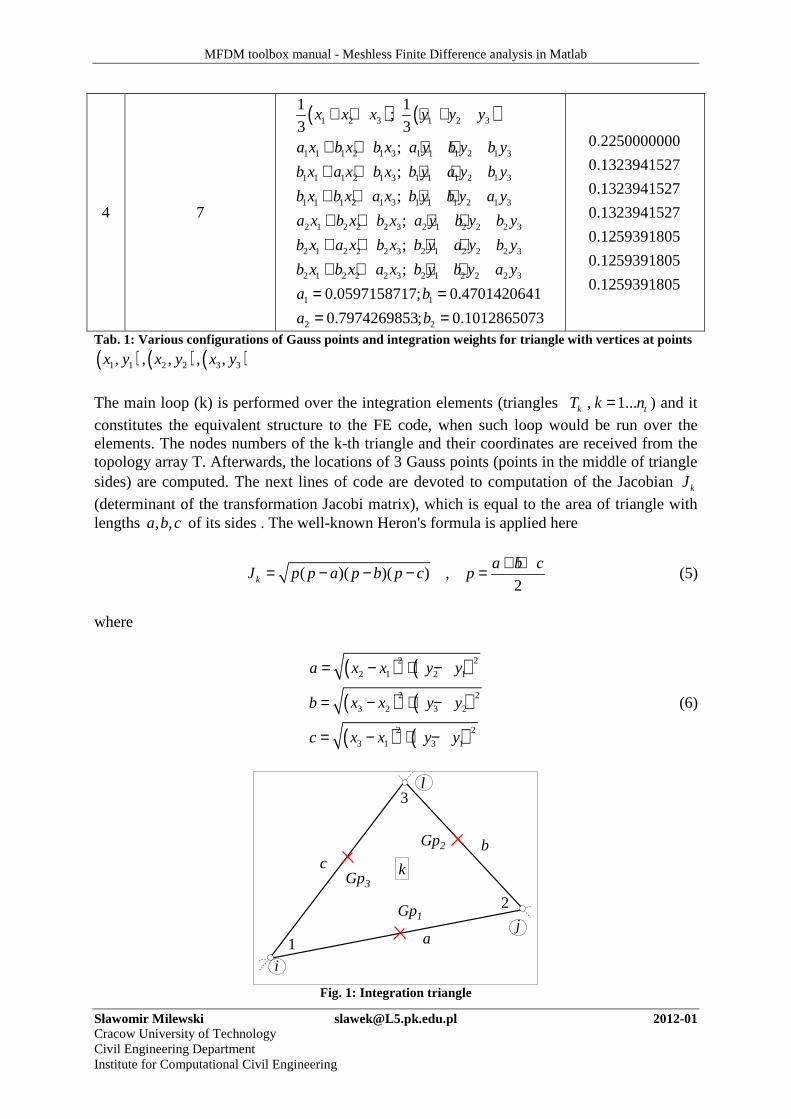
The main loop (k) is performed over the integration elements (triangles , 1...k tT k n= ) and it

constitutes the equivalent structure to the FE code, when such loop would be run over the elements. The nodes numbers of the k-th triangle and their coordinates are received from the topology array T. Afterwards, the locations of 3 Gauss points (points in the middle of triangle sides) are computed. The next lines of code are devoted to computation of the Jacobian kJ

(determinant of the transformation Jacobi matrix), which is equal to the area of triangle with lengths , ,a b c of its sides . The well-known Heron's formula is applied here

( )( )( ) ,2k

a b cJ p p a p b p c p

+ += − − − = (5)

where

( ) ( )

( ) ( )

( ) ( )

2 2

2 1 2 1

2 2

3 2 3 2

2 2

3 1 3 1

a x x y y

b x x y y

c x x y y

= − + −

= − + −

= − + −

(6)

k

i

j

l

1

2

3

a

bc

Gp1

Gp2

Gp3

Fig. 1: Integration triangle



The most interesting part of this code starts from the loop (p) over Gauss points in the specified (k) triangle. The MFD star with additional nodes is generated at every Gauss point using the same distance-based criterion and the same Matlab function (star) as for the local formulation. Moreover, the MFD star still constitutes the one and only support for approximation of the trial function. Here, the order of approximation may be reduced to 1 due to the requirements for the trial function in the variational principle (2). The (mwls) function produces the MF ( ( )FM ) MFD formulas matrix for the trial function F. The approximation support for the test function v differs with the size of the MFD star. The MFD star for the test function v is established for three nearest nodes which are located in vertices of the k-th triangle. This feature is identical for both the MFDM and FEM approaches. The test function v has to be interpolated (matrix Mv - ( )vM ) on the integration subdomain. Otherwise, it provides additional non-zero residual error to the system of MFD equations. It is worth stressing that it does not disrupt the meshlessness of the approach as the integration triangle does not have any influence on the approximation support of the trial function F. It has to be mentioned here, that the triangular integration mesh is only one of the several various approaches for numerical integration in the meshless methods. It was chosen here mainly due to the fact of the simplicity of triangles generation in Matlab (one built-in procedure for Delaunay triangles). The other approaches, which may be associated with the term "meshless" in more direct manner, include the local-global Petrov-Galerkin approaches (proposed by S.Atluri), in which the test function may be constant over the specified subdomain, usually prescribed to each node. Such domain has simple geometrical shape (rectangle, circle) and may determined totally independently from the cloud of nodes. In case of global approach, the aggregation is required. It is performed in the same manner as in the FEM, i.e. in the form of the summation of the matrix and vector terms in each integration subdomain. The appropriate terms of both global matrix A and vector B are aggregated in according to the formulas that result from the discrete form of the variational principle (3)

( ) ( ) ( ) ( ) ( )

1

3 3 3( ) ( ) ( ) ( ) ( )2, 2, 3, 3, 1,

1 1 1 1 1 1 1

2 2

2

t

k

G

k k k k k

n

k T

nt m mF v F v v

k p j i j i ij i j i ik p j i j i i

F v F v F v F vG v d G v dxdy

x x y y x x y y

J M F M v M F M v G M v

θ θ

ω θ

=Ω

= = = = = = =

∂ ∂ ∂ ∂ ∂ ∂ ∂ ∂+ − Ω = + − ≈ ∂ ∂ ∂ ∂ ∂ ∂ ∂ ∂

≈ + −

∑∫ ∫

∑ ∑ ∑ ∑ ∑ ∑ ∑ (7)

Imposition of the homogeneous essential boundary conditions requires additional modification of the global matrix and vector. If BC code of subsequent i-th node is equal to 1, the appropriate i-th row and i-th column of global matrix A and i-th element of B are reset as well as the diagonal i-th element of A is set to 1. This is the same technique as commonly applied in the FEM. It is organized here in the form of several subsequent matrix transformations which will run faster than one loop over all nodes. It may be generalized for non-homogeneous conditions as well. Algorithm is completed by solution of the non-singular set of the MFD equations. Several remarks may be noted



- solution algorithm involves numerical integration, performed here between the nodes over triangles (most effective option for odd order of the differential operators), as in the FEM for triangular elements,

- MFD formulas are computed at Gauss points rather than at nodes, - trial (unknown) function F is approximated on the MFD star with greater number

of nodes than it is required for the assumed approximation order, - approximation order of the trial function may be reduced to 1 (p=1), - test function is interpolated (with order p=1) on the integration subdomain only,

without any additional nodes, - aggregation of both the global matrix and global vector is required and it is

performed in the same manner as in the FEM, - imposition of the essential boundary condition is based on the reconstruction of the

global matrix and vector and it is performed in the same manner as in the FEM. Moreover, above given code may be simply extended for the imposition of the natural boundary condition (e.g. edge loading). The loop over triangles edges is necessary in order to introduce additional elements to the global vector B for those nodes which are located on the boundary subjected to natural conditions.

5. General postprocessing of the results As the result of the solution of the MFD equations, one obtains the nodal values of the Prandtl function F. Here, considered is calculation of the stress components as well as total shear stress (1). The postprocessing may be performed at arbitrary point of the domain or its boundary as well as on the chosen subdomain. In the first case, only local value is sought and it is computed directly by means of the MWLS approximation. In the second case, one need to integrate over chosen subdomain (e.g. triangle or polygon) or over the whole domain. The MWLS approximation is sought then at every Gauss point. Such approach is commonly applied in order to visualize the results in computer programs. Integral values inside the triangles may be also helpful in adaptive analysis. Some additional MWLS techniques, for instance smoothing and filtering of the rough numerical results, may be included as well.

function header: [StrN,StrT,Res] = postprocessingMFDM(N,X,Y,T,nt,F,G,teta) -- Arguments list: N - number of nodes


T (nt x 3)- list of triangles nt - number of triangles

F (N x 1) - nodal values of Prandtl function (primary MFDM solution) G - shear modulus


StrN (N x 3) - array of stresses at nodes: componet tzx, component tzy and total value tz

StrT (nt x 3) - array of stresses at triangles: componet tzx, component tzy and total value tz

Res (nt x 1) - vector of residual error Large parts of already implemented codes may be applied here with small changes only. The list of postprocessing arguments may consist of the same items as in the previous examples, with additional items for the nodal values (vector F) of the primary solution (calculated nodal values of the Prandtl function). Results of both local and variational approaches may be substituted here. The number of nodes for the MFD stars should be greater (e.g. m=16) when



compared with the number applied for the MFD formulas generation. Calculation of nodal stresses requires one loop. At each node, the MFD star and MFD formulas are generated. For the postprocessing, it is recommended to use non-singular weights, e.g. in the form proposed by W.Karmowski

14

22 2

p

i

g

gω ρ

ρ

− −

= + + (8)

where ρ is a distance between central star point and its specified node and g is a small parameter, that defines the rank of the data smoothing. When g ≠ 0, smoothing is applied. When g = 0, no smoothing occurs and the weights in formula (8) become singular (rough interpolation is provided). So far, the mwls function was applied for derivatives approximation and g = 0 in order to impose the interpolation in the central point (e.g. node) of the MFD star (the Kronecker delta property). Here, assumed is g > 0. The MFD formulas are applied in order to obtain the nodal values of the partial derivatives of

the first order F

x

∂∂

and F

y

∂∂

( ) ( )

( ) ( )1, 2,1 1, ,

,i i

i i i i

m m

k kk kk kx y x y

F FM F M F

x y= =

∂ ∂ ≈ ≈ ∂ ∂ ∑ ∑ (9)

which are necessary for computation of stresses (9). Afterwards, the mean integral values (forces) of stresses (9) as well as residual error of the local formulation (2)

2 2

2 22

F Fr G

x yθ∂ ∂= + +

∂ ∂ (10)

are evaluated over each triangle T

, ,T T Tzx zx zy zy

T T T

dxdy dxdy r r dxdyτ τ τ τ= = =∫ ∫ ∫ (11)

As in the case of the standard variational approach, only 3 Gauss points may be assumed. The MFD stars and MFD formulas are generated at every Gauss point in order to approximate the integrals (11). For instance, given is the following discrete value of the global residual error (10) evaluated for triangle T

( )4, 6,1 1

2G

p

n mT

p j j jp j

r J M M F Gω θ= =

≈ + +

∑ ∑ (12)

6. Numerical results

Matlab implementation of the basic steps of the MFDM solution approach was

considered. Examples may concern the following aspects



- the impact of nodes irregularity on the final results, - various domain shapes and construction of the boundary, - various types of benchmark problems (shear analysis, plane stress analysis, plate

deformation etc), - comparison of the results obtained for local and variational formulations, - the effectiveness of the final results postprocessing.

Let us consider a rectangular domain with length (a) and width (b) equal to 2.

Prismatic bar with such rectangular cross-section is subjected to torsion. Appropriate b.v. problem may be posed locally (2) at each point, or globally (3) by means of the variational principle.

In the "TEST.m" file, defined are all parameters required for the proper program functioning. For sake of simplicity, assumed (non-physical) are non-mechanical test values of

G = 1 and 6

πθ = . The variable task may be assumed as "1" or "2". 1 is for the rectangular

domain, whereas 2 is for the railroad rail domain. In case of the rectangular domain (task = 1), the user has to define the dimensions a and b of the rectangle as well as the number of nodes in the x and y directions (parameters nx and ny). The variable formulation is responsible for the b.v.p. formulation type: local ("1") or global (variational weak - "2"). Below presented are the Matlab results for the regular mesh generation in the rectangle after assuming 933 =×=N nodes, with regular spacing 1== yx hh , consequently numbered

from 1 to 9. Thus only one unknown function value (middle node 5) is sought ( ?5 =F ). The

well-known Matlab function meshgrid is applied in order to generate regular mesh in the rectangle, while the array of triangles (T) may be obtained by means of the other Matlab function, delaunay. Potential users are encouraged to run the "TEST.m" file for nx = ny = 3. The proper values of the domain discretization should be as follows

- X = [0 1 2 0 1 2 0 1 2], - Y = [0 0 0 1 1 1 2 2 2], - BC = [1 1 1 1 0 1 1 1 1], - N = 9.

The properly implemented code for local formulation should provide value 0.31415935 =F ,

whereas the variational one should yield 0.4405185 =F . The results for the denser mesh

(with 4002020 =×=N nodes) are as follows. The maximum value of F is equal to 0.30715max =F for the local formulation, whereas it is equal to 0.30832max =F for the

variational one. Additionally, in the "TEST.m" file implemented were some simple visualization procedures. As the result of the program run, one figure appears, divided into the four independent graphs. In each graph, various quantity is shown: the Prandlt function (F), the stress components zxτ

and zyτ as well as the total shear stress zτ . The only Matlab function, which was used here,

is the patch function which draws the filled polygon defined by three vectors of space coordinates as well as one colour parameter.



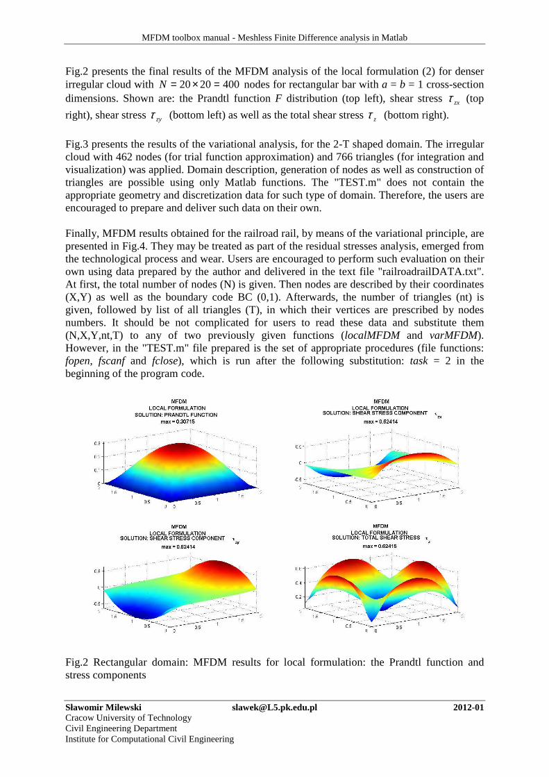
Fig.2 presents the final results of the MFDM analysis of the local formulation (2) for denser irregular cloud with 4002020 =×=N nodes for rectangular bar with a = b = 1 cross-section dimensions. Shown are: the Prandtl function F distribution (top left), shear stress zxτ (top

right), shear stress zyτ (bottom left) as well as the total shear stress zτ (bottom right).

Fig.3 presents the results of the variational analysis, for the 2-T shaped domain. The irregular cloud with 462 nodes (for trial function approximation) and 766 triangles (for integration and visualization) was applied. Domain description, generation of nodes as well as construction of triangles are possible using only Matlab functions. The "TEST.m" does not contain the appropriate geometry and discretization data for such type of domain. Therefore, the users are encouraged to prepare and deliver such data on their own. Finally, MFDM results obtained for the railroad rail, by means of the variational principle, are presented in Fig.4. They may be treated as part of the residual stresses analysis, emerged from the technological process and wear. Users are encouraged to perform such evaluation on their own using data prepared by the author and delivered in the text file "railroadrailDATA.txt". At first, the total number of nodes (N) is given. Then nodes are described by their coordinates (X,Y) as well as the boundary code BC (0,1). Afterwards, the number of triangles (nt) is given, followed by list of all triangles (T), in which their vertices are prescribed by nodes numbers. It should be not complicated for users to read these data and substitute them (N,X,Y,nt,T) to any of two previously given functions (localMFDM and varMFDM). However, in the "TEST.m" file prepared is the set of appropriate procedures (file functions: fopen, fscanf and fclose), which is run after the following substitution: task = 2 in the beginning of the program code.

Fig.2 Rectangular domain: MFDM results for local formulation: the Prandtl function and stress components



Fig.3 2-T shaped domain: MFDM results for variational formulation: the Prandtl function and stress components

Fig.4 Railroad rail domain: MFDM results for variational formulation: the Prandtl function and stress components



7. Comparison with the Finite Element Method algorithm It is worth to compare already obtained results of the MFDM solution approach with the

results obtained by means of the standard Finite Element approximation technique. Let us pay attention on the variational Galerkin type formulation (3), fundamental formulation for the element based discrete approach in most cases. After partitioning of the domain into the set of the non-overlapping elements (triangles, rectangles), it is required to fulfil the variational principle (3) on the finite elements separately. This integral approach may lead to several local matrix and vector quantities (stiffness matrix, mass matrix, load vector etc.) . Afterwards, one needs to aggregate the local quantities in order to produce the global set of algebraic equations. Therefore, the most important features which distinguish standard meshless and standard element based approaches, may be listed as follows:

- element structure is required a-priori, as the main part of the domain discretization,

- both test and trial functions are interpolated by means of the same basis (shape) functions,

- the approximation of the unknown function is prescribed on the element (between the nodes), without any additional nodes or degrees of freedom (no least squares technique is required)

- the interpolation schemes (usually of Lagrange or H'ermite type) are defined in the explicit manner, and do not require evaluation of interpolation values point by point.

Moreover, the MFDM solution approach may be treated as the more general discrete approach, since it allows using of the arbitrary boundary value problem formulation (local, global, mixed), whereas the FEM uses the variational formulations only. In the present paper, two examples of implemented codes were discussed and tested. The second example concerns the variational formulation (3) and the meshless type of solution approach. It uses the triangular background mesh in order to perform the numerical integration (between the nodes). This type of integration is applied in the FEM analysis as well. Therefore, the program code for variational formulation using the meshless FMD and integration between the nodes (using the triangular cells), presented in the previous sections, may be transferred into the finite element code without any difficulties. Here, the only parameter, which has to be modified, is the size of the MFD star (the variable 'm' defined in the beginning of the varMFDM function). It has to be equal to 3. What shall happen then? The number of nodes in the MFD star defined at Gauss points inside the triangles (three nodes located closest to the Gauss point are the triangle vertices) would guarantee function interpolation there (triangular finite elements with the linear interpolation, based on three nodal function values). No additional nodes from outside the triangle will be used, therefore the weight matrix W for the moving least squares approximation will not have any influence on the final results (no additional free degrees are available within the assumed approximation order). The MFD coefficient matrix M, consisting of the MFD formulas for subsequent derivatives up to the assumed p-th, would present the values of the element shape functions at considered the Gauss point. It has to be stresses that in such case, the matrices in function varMFDM code, namely MF and Mv, would be the same (due to the same approximation order 1 and the same number of nodes in the MFD star).



The subsequent steps of the algorithm remain the same as for the MFDM analysis (aggregation, fulfilment of the essential boundary conditions, solution of the set of algebraic equations). However, the postprocessing of the nodal solution is expected to produce rather different results in both cases. Despite the low approximation order (p = 1) applied in case of the MFDM analysis, the stress fields will be continuous (it is presented in Fig.2, Fig.3 and Fig.4), due to the continuous global approximation (only the local approximation of the 1st order remains discontinuous). This feature will not occur in case of the FEM analysis conducted using software devoted to the FEM only. The stress fields should remain discontinuous due to the 0C linear interpolation of the unknown function, unless any additional smoothing is applied. That is not the case here. Software delivered here reproduces the continuous derivatives fields using the MWLS approximation in each case. It is important to mention that only this type of MFDM analysis may be reduced to the FEM analysis by means of the small code modification only. The other criteria of nodes selections for the MFD star or the other integration techniques may lead to the different results, especially for the coarse meshes and may not have equivalent element based approach. Below presented are results of the FEM analysis of the prismatic bar with the rectangular cross-section a = b = 2 (task 1)

- for 3 3 9N = × = nodes, maxF = 0.34907,

- for 20 20 400N = × = nodes, maxF = 0.30475.

No additional figures (for the FEM results) are shown here due to the fact that for every domain type and for the fine mesh with 400 nodes, individual graphs (e.g. Prandlt function F distribution for local MFDM, variational MFDM and FEM) are very closed to each other. Therefore, some deeper and comprehensive discussion concerning efficiency of the meshless and element based approaches as well as reasonable a-posteriori error estimation should be added. This should be the topic of the separate paper and the associated software and its instruction. However, it is worth to compare those results with the ones obtained for the variational principle (3) using the MFDM solution approach. Moreover, further MFDM and FEM calculations may be performed using delivered software, e.g. for different domain geometry and various number of nodes.

Documents

Meshless Finite Difference Method analysis in Matlab ...static-content.springer.com/esm/art:10.1007/s11075-012-9614-6... · solution approach into the Matlab code. ... as the specific