MESHFREE FORMULATIONS OF KINEMATIC WAVE FOR …eprints.utm.my/id/eprint/78724/1/HalinawatiHirolPFKA2016.pdf · persamaan ombak kinematik St Venant untuk model hidrologi air larian

MESHFREE FORMULATIONS OF KINEMATIC WAVE FOR CHANNEL

FLOW ROUTING

HALINAWATI BINTI HIROL

A thesis submitted in fulfilment of the

requirements for the award of the degree of

Doctor of Philosophy (Civil Engineering)

Faculty of Civil Engineering

Universiti Teknologi Malaysia

SEPTEMBER 2016

To my thoughtful and lovely husband, parents, children and family.

ii

ACKNOWLEDGEMENT

Praise to Allah, the All Mighty who sparks my intuition to pursue my PhD

study and provides me with invaluable guidance throughout my study and life.

Thanks to Universiti Teknologi Malaysia and the Government of Malaysia,

for providing the financial support throughout my study.

Thanks to my supervisor, Prof. Dr Zulkifli Yusop and Dr Ahmad Kueh Beng

Hong for their supervision and support in seeing this work through to completion.

For my lovely husband, Dr Airil Yasreen Mohd Yassin and cheerful kidsAiril

Haziq, Hasya ‘Ainaa, Nuha Liyana and Hafsa Binish, thanks for cheering up my life.

To my past parent, Hirol Bol Hasan and Salbia Jini, my parent in law, Mohd

Yassin Shariff and Halimah Saidin and my family, my deepest appreciation goes out

to all of you.

Thanks also to all my research colleagues especially Mohd Zafri Jamil Abd

Nazir and Mohd Al-Akhbar Mohd Noor for their work support and assistances.

iii

ABSTRACT

This study concerns the development of various Meshfree formulations,

namely Point Interpolation Method (PIM), Radial Point Interpolation Method

(RPIM) and Element Free Galerkin (EFG) in solving numerically, St Venant’s

kinematic wave equations for the hydrologic modeling of surface runoff and channel

flow. It involves problem formulations derivation of governing equations, provision

of the corresponding solutions by generating Matlab source codes, verification of

results against established data, parametric study and assessment of performance of

the newly derived Meshfree formulations against established numerical methods,

namely Finite Element Method (FEM) and Finite Difference Method (FDM). The

originality and the main contribution of the study are solving the Meshfree

formulations of the kinematic wave equations numerically. The formulations are

verified when it is found that the results produced by the source codes are in general

in close agreement with the benchmark data. Although slight discrepancies have

been observed in some cases, these are later validated as due to several factors,

namely shape parameters values which are yet to be optimized, different number of

nodes used for comparison and manual discretization of input data. In obtaining the

best performance of the methods, optimum values of the shape parameters have been

determined through a parametric study which once obtained are used in the

performance assessment. RPIM and PIM are found to be less sensitive to the

optimum values as compared to EFG. Two types of performance are assessed; the

convergence rate and the computer resource consumption in terms of CPU time.

Based on this study, it can be concluded that, in general, Meshfree methods perform

comparably with the established methods in terms of convergence rate despite the

fact it does not need the construction of mesh which can save modelling time. This

shows the potential of Meshfree as numerical methods for its future development.

iv

ABSTRAK

Kajian ini adalah berkenaan penerbitan formulasi beberapa kaedah Meshfree

iaitu Point Interpolation Method (PIM), Radial Point Interpolation Method (RPIM)

dan Element Free Galerkin (EFG) dalam menyelesaikan secara numerikal

persamaan ombak kinematik St Venant untuk model hidrologi air larian permukaan

dan aliran alur. Kajian ini melibatkan penerbitan formulasi, penyediaan penyelesaian

dan penulisan kod komputer menggunakan Matlab, pengesahan keputusan melalui

perbandingan dengan data sediada, kajian parameter dan penilaian kemampuan

kaedah-kaedah yang baharu dihasilkan melalui perbandingan dengan kaedah-kaedah

numerikal sediada seperti kaedah unsur terhingga dan kaedah pembeza. Keaslian dan

sumbangan utama kajian ini adalah formulasi beberapa kaedah Meshfree yang

dihasilkan dengan menukar persamaan ombak kinematik ke dalam bentuk matrik.

Formulasi-formulasi yang diterbitkan telah disahkan apabila keputusan-keputusan

yang terhasil didapati menyamai data sediada. Walaupun terdapat perbezaan kecil

untuk beberapa kes, ia telah dijelaskan sebagai kesan dari beberapa faktor seperti

nilai parameter bentuk yang belum optimum, perbezaan bilangan nod sewaktu

perbandingan dibuat dan penentuan input data sediada yang dibuat secara manual.

Kemampuan terbaik kaedah-keadah yang baharu dihasilkan ini diperoleh dengan

penentuan nilai optimum parameter bentuk melalui kajian parameter yang telah

dijalankan. PIM dan RPIM didapati kurang dipengaruhi oleh nilai optimum

berbanding EFG. Melalui penggunaan nilai-nilai optimum ini, kajian kemampuan

telah dijalankan dimana ia melibatkan dua bentuk kajian iaitu kadar penumpuan dan

kadar penggunaan sumber komputer. Berdasarkan kajian ini boleh disimpulkan

bahawa secara umumnya kaedah-kaedah Meshfree mempunyai kemampuan yang

sama dengan kaedah-kaedah numerikal sediada walaupun ia tidak memerlukan

penyediaan mesh lantas mengurangkan masa untuk kerja permodelan dan ini

menunjukkan potensi untuk penggunaan akan datang.

vii

TABLE OF CONTENTS

CHAPTER TITLE PAGE

DECLARATION ii

DEDICATION iii

ACKNOWLEDGEMENTS iv

ABSTRACT v

ABSTRAK vi

TABLE OF CONTENTS vii

LIST OF TABLES xiii

LIST OF FIGURES xiv

LIST OF SYMBOLS xx

LIST OF APPENDICES xxiii

1 INTRODUCTION 1

1.1 Kinematic Wave Equation 1

1.2 Numerical Methods 2

1.3 Meshfree Methods 4

1.4 Problem Statement 5

1.5 Objectives of Study 6

1.6 Scope and Limitation of Study 7

1.7 Significance of Study 8

viii

1.8 Outline of Thesis 8

2 LITERATURE REVIEW 11

2.1 Introduction 11

2.2 Deterministic Modeling Approach 11

2.3 Characteristic of the Kinematic Wave

Equations 13

2.4 Numerical solutions of Kinematic Wave

Equations 14

2.4.1 Finite Difference Method 15

2.4.2 Finite Element Method 17

2.5 Meshfree Methods 18

2.5.1 Point Interpolation Method (PIM) 22

2.5.2 Radial Point Interpolation Method

(RPIM) 22

2.5.3 Element Free Galerkin (EFG) 23

2.6 Meshfree Shape Parameters 24

2.7 Application of Meshfree in Hydrologic

Modelling 25

2.8 Concluding Remarks 27

3 METHODOLOGY 29

3.1 Introduction 29

3.2 Saint Venant’s Kinematic Wave Equation 29

3.3 Galerkin Weighted Residual

Method of Kinematic Wave 32

3.3.1 Iterative Schemes for Nonlinear

Solutions 35

3.3.1.1 Picard’s Scheme 35

3.3.1.2 Newton-Raphson’s Scheme 37

ix

3.3.1.3 Tangent Stiffness Matrix 41

3.4 Finite Difference Formulation 44

3.5 Finite Element Shape Functions 47

3.5.1 Quadratic Shape Functions 47

3.6 Point Interpolation Method (PIM) Shape Functions 50

3.6.1 Evaluated Values of PIM Shape Functions 53

3.7 Radial Point Interpolation Method (RPIM)

Shape Functions 56

3.7.1 Evaluated Values of RPIM Shape Functions 59

3.8 EFG with Moving Least Square

Shape Functions 61

3.9 Derivative of Meshfree Shape Functions 66

3.9.1 First Derivative of PIM Shape Functions 66

3.9.2 First Derivative of RPIM Shape Functions 68

3.9.3 First Derivative of MLS Shape Functions 70

3.10 Meshfreee Weak Form Formulation 71

3.10.1 Meshfree Formulation in Gauss

Quadrature Scheme 72

3.11 Concluding remarks 76

4 VALIDATION OF MESHFREE FORMULATIONS 78

4.1 Introduction 78

4.2 Validation of Formulations 79

4.2.1 Chow et.al (1988) 80

4.2.1.1 Validation of Finite Element

Method (FEM) Formulation 82

4.2.1.2 Validation of Finite Difference

Method (FDM) formulation 85

4.2.1.3 Validation of Point Interpolation

Method (PIM) formulation 88

4.2.1.4 Validation of Radial Point

x

Interpolation Method (RPIM)

Formulation 90

4.2.1.5 Validation of Element Free

Galerkin (EFG) formulation 93

4.2.2 Vieux et. al (1990) 96



4.2.2.2 Validation of Finite Difference

Method (FDM) formulation 100





Formulation 103



4.2.3 Litrico et. al (2010) 106







Formulation 111




5 PARAMETRIC AND CONVERGENCE

STUDIES OF MESHFREE FORMULATIONS 115

5.1 Introduction 115

5.2 Parameter Effects on PIM 116

xi

5.2.1 Effect of The Size of Support

Domain αs 118

5.2.2 Effect of the number of Gauss Point

on PIM 120

5.3 Parameter Effects on RPIM 123

5.3.1 Effect of The Shape Parameter

And on RPIM 124

5.3.2 Effect of the size of support

domain, on RPIM 128

5.3.3 Effect of the Number of Gauss Point,

GP on RPIM 130

5.4 Parameter Effects on EFG 132

5.4.1 Effect of The Size of Support

Domain, on EFG 133

5.4.2 Effect of Number of Gauss Point,

GP on EFG 135

5.5 Convergence Study 137

5.5.1 Convergence Study Using

Newton-Raphson 138

5.5.2 Convergence Study for Picard 141

5.5.3 Convergence Study Between Two

Iterative Scheme 144

5.6 Performance Study in Terms of Computer

Resource 146

5.6.1 CPU Times Consumption 148

5.7 Validation Using Optimum Values 151


6 SUMMARY AND CONCLUSIONS 157

6.1 Introduction 157

6.2 Summary of Study 157

6.3 Conclusions of Study 158

xii

6.4 Suggestions for Future Works 160

REFERENCES 161

Appendices A-N 169 - 270

xiii

LIST OF TABLES

TABLE NO. TITLE PAGE

2.1 Differences between FEM and Meshfree method

(Liu and Gu, 2005)

21

4.1 Chow’s input data 81

4.2 Parameter of the study by Litrico et. al (2010) 107

5.1 Optimum ranges and value of αs of PIM 120

5.2 Optimum ranges and value of GP of PIM 123

5.3 Optimum ranges and value of of RPIM 126

5.4 The chosen value for shape parameter based

on three benchmark studies

128

5.5 Optimum ranges and values of of RPIM 130

5.6 The chosen value for Gauss Point based on three

benchmark studies

132

5.7 Optimum ranges and values of of EFG 135

5.8 Optimum ranges and values of GP of EFG 136

5.9 Values for PIM Shape Parameters 151

5.10 Values for RPIM Shape Parameters 152

5.11 Values for EFG Shape Parameters 152

xiv

LIST OF FIGURES

FIGURE NO. TITLE PAGE

2.1 Flowchart for the FEM and Meshfree methods

20

3.1 Bed slope So and the frictional slope Sf with y

depth

31

3.2 Picard scheme step by step procedure flowchart

36

3.3 Newton-Raphson scheme step by step procedure

flowchart

40

3.4 Degree of freedoms of quadratic elements

48

3.5 Quadratic shape functions

50

3.6 Typical domain discretization by PIM

55

3.7 Plots of PIM shape functions at a typical point of

interest

55

3.8 Plots of PIM shape function using various

numbers of points of interest

55

3.9 Plots of RPIM shape functions at a typical point

of interest

61

3.10 Plots of RPIM shape function using various


61

3.11 Plots of MLS shape functions at a typical point of

interest

65

3.12 Plots of MLS shape function using various


66

3.13 Mapping of physical domain (flow domain) to

natural domain

73

xv

4.1 The point uniformly distributed along the channel

82

4.2 Newton-Raphson Nonlinear FEM at point 6000 of

Chow (1988)

83

4.3 Newton-Raphson Nonlinear FEM at point 12000

ft of Chow (1988)

84

4.4 Picard Nonlinear FEM at point 6000 ft of Chow

(1988)

84

4.5 Picard Nonlinear FEM at point 12000 ft of Chow

(1988)

85

4.6 Newton-Raphson Finite Difference Model at

point 6000 ft

86

4.7 Newton-Raphson Finite Difference Model at

point 12000 ft

86

4.8 Picard Nonlinear Finite Difference Model at point

6000 ft

87

4.9 Picard Nonlinear Finite Difference Model at point

12000 ft

87

4.10 Newton-Raphson Nonlinear PIM at point 6000 ft

88

4.11 Newton-Raphson Nonlinear PIM at point 12000 ft

89

4.12 Picard Nonlinear PIM at point 6000 ft 89

4.13 Picard Nonlinear PIM at point 12000 ft 90

4.14 Newton- Raphson Nonlinear RPIM at point 6000

ft

91

4.15 Newton- Raphson Nonlinear RPIM at point 12000

ft

91

4.16 Picard Nonlinear RPIM at point 6000 ft 92

4.17 Picard Nonlinear RPIM at point 12000 ft 92

4.18 Newton-Raphson Nonlinear EFG at point 6000 ft

94

xvi

4.19 Newton-Raphson Nonlinear EFG at point 12000

ft

94

4.20 Picard Nonlinear EFG at point 6000 ft 95

4.21 Picard Nonlinear EFG at point 12000 ft 95

4.22 One-Dimensional Element Representation of Two

Plane Watershed (Vieux et. al, 1990)

97

4.23 Newton-Raphson Nonlinear Finite Element versus

Vieux et. al (1990)

99

4.24 Picard Nonlinear Finite Element versus Vieux et.

al (1990)

99

4.25 Descritized plane with many numbers of finite

difference points

100

4.26 Newton-Raphson Nonlinear Finite Difference

versus Vieux et. al (1990)

101

4.27 Picard Nonlinear Finite Difference versus Vieux

et. al (1990)

101

4.28 Newton-Raphson Nonlinear PIM versus Vieux et.

al (1990)

102

4.29 Picard Nonlinear PIM versus Vieux et. al (1990)

103

4.30 Newton-Raphson Nonlinear RPIM versus Vieux

et. al (1990)

104

4.31 Picard Nonlinear RPIM versus Vieux et. al (1990)

104

4.32 Newton-Raphson Nonlinear EFG versus Vieux et.

al (1990)

105

4.33 Picard Nonlinear EFG versus Vieux et. al (1990)

106

4.34 Upstream flow (Litrico et. al, 2010) 107

xvii

4.35 Newton-Raphson Nonlinear FEM versus

Simplified Nonlinear Modeling based on data

from Litrico et.al (2010)

108

4.36 Picard Nonlinear FEM versus Simplified

Nonlinear Modeling based on data from Litrico

et.al (2010)

109

4.37 Newton-Raphson Nonlinear PIM versus

Simplified Nonlinear Modeling based on data


110

4.38 Picard Nonlinear PIM versus Simplified

Nonlinear Modeling based on data from Litrico

et.al (2010)

110

4.39 Newton-Raphson Nonlinear RPIM versus

Simplified Nonlinear Modelling based on data


111

4.40 Picard Nonlinear RPIM versus Simplified

Nonlinear Modelling based on data from Litrico

et.al (2010)

112

4.41 Newton-Raphson Nonlinear EFG versus

Simplified Nonlinear Modelling based on data


113

4.42 Picard Nonlinear RPIM versus Simplified

Nonlinear Modelling based on data from Litrico

et.al (2010)

113

5.1 Effect of αs to PIM for Chow (1988) 118

5.2 Overall effect of αs to PIM 119

5.3 Effect of Gauss Point, GP to PIM for Chow et.al.

(1988).

121

5.4 Overall effect of Gauss Point, GP to PIM 122

5.5 Effect of shape parameter to RPIM for Chow

et.al. (1988)

125

5.6 Overall effect of shape parameter to RPIM 126

5.7 Shape parameter in Chow’s benchmark

problem

127

5.8 Result of shape parameter against the norms of

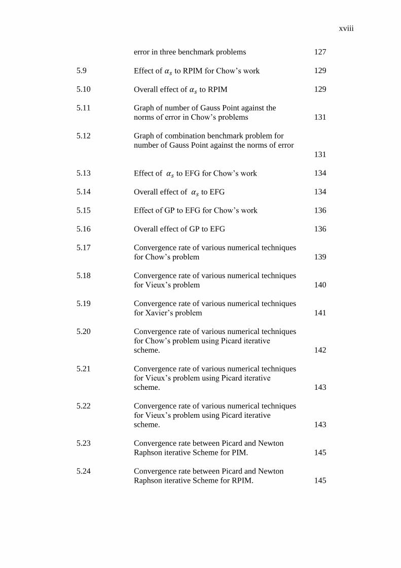
xviii

error in three benchmark problems 127

5.9 Effect of to RPIM for Chow’s work 129

5.10 Overall effect of to RPIM 129

5.11 Graph of number of Gauss Point against the

norms of error in Chow’s problems

131

5.12 Graph of combination benchmark problem for

number of Gauss Point against the norms of error

131

5.13 Effect of to EFG for Chow’s work 134

5.14 Overall effect of to EFG 134

5.15 Effect of GP to EFG for Chow’s work 136

5.16 Overall effect of GP to EFG 136

5.17 Convergence rate of various numerical techniques

for Chow’s problem

139


for Vieux’s problem

140


for Xavier’s problem

141


for Chow’s problem using Picard iterative

scheme.

142


for Vieux’s problem using Picard iterative

scheme.

143


for Vieux’s problem using Picard iterative

scheme.

143

5.23 Convergence rate between Picard and Newton

Raphson iterative Scheme for PIM.

145


Raphson iterative Scheme for RPIM.

145

xix


Raphson iterative Scheme for EFG.

146

5.26 Time consume for various numerical technique to

converge using Picard iterative scheme for

Litrico’s work

148

5.27 Comparison between two iterative schemes for

PIM formulation

149


RPIM formulation.

150


EFG formulation

150

5.30 Comparison between values of shape parameters

for PIM formulation

153


for for RPIM formulation

154


for EFG formulation

154

xx

LIST OF SYMBOLS

- cross-sectional area of the flow

BC - background cell

GP - number of gauss point

- gravitational pull

- Length of domain

- the number of polynomial terms used in RPIM

interpolation

n - number of the field node in the support domain

- Wetted perimeter

- flow rate

- MQ-RBF dimensionless shape parameter

- forcing term (i.e. precipitation, lateral flow).

- iteration

- Time

x - spatial coordinate

- depth of water

- size of spatial increment

- time step

- ( ( √ ))

- 0.6 (factor in Manning equation)

- Manning roughness coefficient

xxi

- error criterion

- MLS interpolation potential

- natural coordinate

- Matlab command for Gauss elimination procedure

- size of support domain

- averaged distance between adjacent nodes

- distance from node to the point of interest

(i.e. | | )

- shape functions

- degree of freedoms (nodal values) of flow rate

- frictional slope

- bed slope

- coordinates of point of interest

point of interest

αs - size of support domain

αc - MQ-RBF dimensionless shape parameter

- Kronecker delta

[ ] - weighted moment matrix

- MLS non-constant coefficient

{ } - vector of interpolation coefficient

{ } - Vector of polynomial coefficients in RPIM

interpolation

{ } - load vector

[ ] - stiffness matrix

[ ] - mass matrix

{ } - vector of degree of freedoms

xxii

{ } - residual of partial differential equations

{ } - incremental degree of freedoms

[ ] - tangent stiffness

- residual error in finite difference scheme

{ } - vector of monomials built from Pascal triangle

[ ] - evaluated values of the monomials at nodes (also

termed as PIM moment matrix)

{ } - shape functions evaluated at point of interests

{ } - monomials evaluated at point of interests

{ } = - vector of radial basis function (RBF)

{ } - vector of radial distance of point of interest

[ ] - evaluated radial basis function at nodes

[ ] - RPIM moment matrix

{ } - Evaluated values of { } and { } at point of interests

[ ] - MLS weight functions

| | - Jacobian for fth

background cell

- Gauss weighting factor for the gth

Gauss point

xxiii

LIST OF APPENDICES

APPENDIX TITLE PAGE

A Derivation of Saint Venant equation using

Reynold Transport Theorem

169

B Derivation of PIM shape function 174

C Derivation of RPIM shape function 179

D Derivation of MLS shape function 185

E Numerical integration example: 190

F FEM code for Saint Venant’s kinematic wave

equation using Newton-Raphson iterative

scheme

200

G FEM code for Saint Venant’s kinematic wave

equation using Picard iterative scheme

207

H FDM code for Saint Venant’s kinematic wave


scheme

214

I PIM code for Saint Venant’s kinematic wave


scheme

217

xxiv

J PIM code for Saint Venant’s kinematic wave


225

K RPIM code for Saint Venant’s kinematic wave


scheme

234

L

RPIM code for Saint Venant’s kinematic wave


243

M EFG code for Saint Venant’s kinematic wave


scheme

253

N EFG code for Saint Venant’s kinematic wave


261

CHAPTER 1

INTRODUCTION

1.1 Kinematic Wave Equations

Hydrologic modeling concerns the study of hydrologic processes such as

evapotranspiration, subsurface flow, surface runoff and channel flow. Methods of

study can be either stochastic or deterministic or combination of the two. Whilst

stochastic method employs probabilistic (statistical) approach, deterministic method

basically involves attempt to solve a set of partial differential equation which

describes the behavior of the flow. This study concerns the latter.

The deterministic approach, on the other hand can be further divided into two

groups, lumped and distributed. The main advantage of distributed modeling over

lumped is that, it is easier to allow for variation in the properties of parameters such

as variation in cross-sectional area, intensity of precipitation, soils coefficients,

slopes and many others.

However, such an advantage requires the solution of a set of one-dimensional

nonlinear partial differential equations known as St. Venant equations. These

2

equations are actually the simplification of the two-dimensional shallow water theory

derived from the general Navier-Stokes equations.

St. Venant equations themselves can be further classified into full dynamics,

diffusive and kinematic wave equations. Full dynamics equations allow for complete

consideration of the flow, whilst diffusive equations able to capture backwater effect.

If the slope of the plane is assumed as equaled to the frictional slope, such an

assumption would uncouple the continuity equation from the momentum equation

hence the prevalence of the kinematic wave equations.

Despite being the simplest case of St Venant equations, there is no closed

form solution available for the kinematic wave except for the simplest case of no

lateral flow and constant wave celerity. The difficulty is due to the nonlinearity as

well as the unsteady state of the equation. As a result, kinematic wave equations are

commonly solved numerically with the help of computer programming.

1.2 Numerical Methods

Physical phenomenon is usually described by a set of partial differential

equations (PDEs). By solving the equations, information of interest can be obtained.

For simple set of equations, closed form solution may be available. But, for complex

problems, solutions are commonly obtained by solving the equations numerically

rather than analytically. Methods used in obtaining such solutions are classified as

numerical methods.

At present, there are various numerical methods have been developed such as

Finite Difference Method (FDM), Finite Element Method (FEM), Boundary Element

3

Method (BEM), Finite Volume Method (FVM) and many more. Amongst these

methods, the most established and famous are FDM and FEM.

FDM can be considered as the earliest form of numerical method which

history of development can be traced back as early as 1930’s (Thomee, 2001). The

basic idea of FDM is to convert the continuous nature of PDE into algebraic

equations in matrix forms by replacing the derivative terms with forward, backward

or central difference equations. The advantage of FDM relies on its straightforward

implementation as well as on the fact that it operates directly of the PDEs, hence the

term strong form. However, the disadvantage of FDM is in the modeling of irregular

domain. Although there are several mapping techniques have been developed, these

techniques are not as convenient as FEM when it comes to modeling irregular

domain.

FEM, as mentioned, is a numerical method which advantage is in its

efficiency in modeling irregular body shapes and problem domains. Such efficiency

is due to the use of interpolation functions to approximate the problems variables.

Historically, FEM was developed during the 1950’s (Bathe, 1996). Whilst the first

reported work on FEM can be attributed to the work of the famous mathematician, R.

Courant in 1943, the major development of the method, especially in the engineering

fields began with the work of Turner et.al (1956) and the separate work by Argyris

and Kelsey (1954). The basic idea in FEM is to discretize the continuous nature of

the PDEs by weaken into a weak statement. This can be obtained by employing

either weighted residual approach or variational approach. Either approach will yield

similar algebraic equations in matrix forms. With the advent of computer

technology, FEM has become an established numerical methods applied in various

fields to include engineering, physics, chemistry and biology (Mackerle, 2002).

Despite the establishment of FDM and especially FEM, researches have been

conducted in finding new numerical methods and looking at other possibilities for

better algorithms. The most notable would be BEM which development was at its

4

height in the 1970’s (Brebbia and Dominguez, 1977). The basic idea of BEM is to

convert the continuous nature of the PDEs by conducting integration by parts until

the differential operators on the unknown variables completely transferred onto the

weighting functions. Such act allows the problem to be defined by the boundary

terms only. However, this method suffered from the need to employ fundamental

solutions or Green functions as the weighting functions which are difficult to be dealt

with.

Further research works in the field of numerical method development then led

to the introduction of a new family of numerical methods termed as Meshfree or

Meshless methods in the 90’s (Liu and Gu, 2005). This is the interest of this study

thus is discuss next.

1.3 Meshfree Methods

Meshfree methods can be considered as the latest output in the research

development of numerical techniques. The inventions were motivated by the attempt

to remove the need for predefined meshes which are required in FEM. It is argued

that, with the removal of the mesh, computer cost in the mesh development as well as

in mesh refinement can be omitted. Therefore, since there could be various ways in

doing this, Meshfree methods do not refer to specific method but to a family of

methods. Methods that fall under this family, amongst others are; Point Interpolation

Method (PIM), Radial Point Interpolation Method (RPIM), Element Free Galerkin

(EFG), Smooth Particle Hydrodynamic (SPH), Meshless Local Petrov Galerkin

(MLPG), Diffuse Element Method (DEM), and Boundary Node Method (BNM).

However, due to constraints, this study only considers PIM, RPIM and EFG.

5

Since Meshfree methods do not require predefined mesh, the construction of

shape functions must be carried out afresh for every analysis. This then becomes the

major work in any Meshfree formulations. In PIM, the shape functions are

constructed by using polynomial interpolation whilst in RPIM, a special interpolation

is employed termed as radial basis function. For EFG, the construction of the shape

functions involve the use of quartic function and the imposition of stationary

condition of weighted discrete norms. All these are going to be detailed in the

upcoming chapter.

Another major topic in the development of PIM, RPIM and EFG is the effect

of several parameters during the construction of the shape functions. Optimum

values of the parameter are required which are best determined by conducting a

series of numerical test on a typical problem as these values can be different from

one case to another (Liu and Gu, 2005).

Since Meshfree methods, especially PIM, RPIM and EFG, are relatively new,

more studies are needed to investigate the robustness and generality of the methods

especially in practical application (Liu and Gu, 2005).

1.4 Problem Statement

The hydrologic phenomenon of surface runoff and channel flow can be

studied by solving kinematic wave equation. However, due to the nonlinearity and

the unsteady state of the equation, no closed form solution is available except for the

simplest case of no lateral flow and constant wave celerity. Therefore, in obtaining a

more general solution, at present, kinematic wave equation is commonly solved

either by using FDM (Chow et.al, 1988) or FEM (Vieux et.al (1990), Litrico et.al

(2010)).

6

However, despite the various works and formulations of FDM and FEM on

kinematic wave equation, there are yet PIM, RPIM and EFG formulations for the

equation. Such undertake is thus important as not only can it provide alternative

methods in the field of hydrology but also assists in the establishment of the

Meshfree methods by widening its study and development into the field of civil

engineering, in particular hydrology and river engineering. Also, by carrying out

such undertaking, the study can also be among the first to provide data on optimum

values of parameters which govern the performance of the Meshfree methods

especially in the field of hydrology and river engineering.

Based on these, it is therefore the main interest and purpose of this study to

the develop PIM, RPIM and EFG formulations for kinematic wave equation.

1.5 Objectives of Study

i. To derive and formulate PIM, RPIM and EFG formulations for kinematic

wave equation and write the corresponding Matlab source-codes. For

performance assessment purposes, source codes for FEM and FDM are also

written.

ii. To validate the formulation against previous works (benchmark problems)

iii. To conduct parametric study (numerical test) to determine the optimum range

and value of parameters in ensuring the best performance of the Meshfree

methods

7

iv. To conduct performance study in terms of convergence rate and computer

resource consumption in assessing the potential of the Meshfree methods

against the established numerical methods; FDM and FEM

1.6 Scope and Limitation of Study

i. To limit the scope of the study, only three type of Meshfree methods are

considered which are PIM, RPIM and EFG

ii. The study strictly involves with mathematical derivations and computer

programming thus no direct experimental works are conducted due to

time constraint. However, the absence of direct experimental work is

compensated by the validation and verification which are carried out

against the actual gauged data provided by one of the benchmark problem

iii. All assumptions in St Venant equations and kinematic wave equation

holds

iv. Although one of the main advantage of Meshfree methods is in the ease

of treating irregular arrangement of nodes hence refinement process, due

to the pioneering nature of this study, only uniform distribution of nodes

is considered and no consideration is given in the refinement process

v. Despite the availability of various nonlinear schemes and time-integration

methods available, this study only employs Picard and Newton-Raphson

as iterative schemes and backward difference as the time-integration

methods because of their simplicity but good convergence.

vi. Despite the availability of various radial basis functions and spline

functions for the construction of shape functions of RPIM and EFG

8

respectively, this study only employ multi-quadric function for the former

and quartic spline function for the latter because they are the most basic

function and generally used.

1.7 Significance of Study

This study is one of pioneering work of PIM, RPIM and EFG methods in

hydrologic modeling especially in the solution of kinematic wave. It provides insight

into the performance of the methods mentioned in terms of convergence rate and

computer resource consumption as well as one of the first to report on the optimum

ranges and values of parameters of the methods. Such information would be useful,

not only for future studies of Meshfree as numerical methods but also in practical

realm of civil engineering and hydrology.

1.8 Outline of Thesis

This thesis comprises of six chapters outlined as follows.

CHAPTER 1: This chapter introduces the general idea of hydrologic

modeling and corresponding methods of study. It describes

relevant theories and equations. An introduction is also

given on various numerical methods to include their brief

history, basic idea and current state of development and

application. Problem statement in then outlined in detailing

the need for the study to be conducted followed by the

9

objectives of the study. To clarify the framework of the

study, scope and limitation are detailed out. The

significance of study is then highlighted.

CHAPTER 2: In this chapter, relevant previous works are reviewed and

discussed. The discussion begins with works related to St

Venant equations especially on kinematic wave equation.

Then, previous works on FDM and FEM related to the

solution of the equation are reviewed and discuss. The final

part of the chapter focuses on the current state of knowledge

on Meshfree methods especially PIM, RPIM and EFG.

CHAPTER 3: This chapter concerns the mathematical derivations of both,

the kinematic wave equation and the relevant numerical

formulations. Established numerical method are derived

first; FEM followed by FDM. Then detailed derivation of

the shape functions leading to the discretized algebraic

equations in matrix forms are given for PIM, RPIM and

EFG.

CHAPTER 4: In this chapter, all formulations and their corresponding

source codes are validated by comparing their results against

three benchmark problems; Chow et. al. (1988), Vieux et.al

(1990) and Litrico et.al (2010). Reasons for the selection of

these problems as benchmark are detailed. Besides

validation of the formulation, validation on the use of

different iterative schemes is also provided.

CHAPTER 5: This chapter is divided into two parts. The first parts

concerns the parametric studies in which series of numerical

tests are conducted in determining the optimum ranges and

values of parameters affecting the performance of the

Meshfree methods. In the second parts, the optimum values

10

are then used in the formulation to assess the performance of

the Meshfree methods relative to the established ones (FDM

and FEM). Their performance in terms of convergence rate

and computer resource consumption (CPU time) are

assessed.

CHAPTER 6: This is the final chapter of the thesis. In this chapter,

findings obtained from the study are summarized and

concluded. Suggestions for future works are given at the

end of the chapter.

160

6.4 Suggestions for Future Works

As mentioned, this study is a pioneering work in the discretization of

kinematic wave equations by Meshfree methods specifically PIM, RPIM and EFG.

Due to its pioneering nature, this work has limitations which can be extended in

future works. It is suggested that the formulations be extended:

i. To allow for irregular distribution of nodes and automated for adaptive

analysis where decision on the distribution and number of nodes is

automatically made based on the needs of the analysis i.e. at the region of

high gradient, moving boundaries, discontinuities etc.

ii. For network system where a number of branches (representing watershed

draining or rivers) can be modeled. This will make the formulation more

general and able to capture greater spatial variability of parameters.

iii. To other forms of St. Venant equations namely diffusion and full

dynamics as this will make the formulation more general and practical

(i.e. allow backwater)

iv. To other Meshfree methods such as smoothed particle hydrodynamics

(SPH) and Reproducing Kernel Particle Method (RKPM).

REFERENCES

Abbott, M. B., & Ionescu, F. (1967). On the numerical computation of nearly

horizontal flows. Journal of Hydraulic Research, 5(2), 97-117.

Amein, M., & Fang, C. S. (1970). Implicit flood routing in natural channels. Journal

of the Hydraulics Division. 96(12), 2481-2500

Argyris, J. H., & Kelsey, S. (1954). Energy theorems and structural Analysis. Part II.

Application to thermal stress problem and Saint Venant's torsion.Aircraft

Engng, 26, 413-416.

Balloffet, A. (1969). One-dimensional analysis of floods and tides in open

channels. Journal of the Hydraulics Division, 95(4), 1429-1454.

Baltzer, R. A., & Lai, C. (1968). Computer simulation of unsteady flows in

waterways. Journal of the Hydraulics Division, 94(4), 1083-1120.

Bathe, K. J. (1996). Finite element procedures. Klaus-Jurgen Bathe.

Belytschko, T., Krysl, P., & Krongauz, Y. (1997). A three‐dimensional explicit

element‐free galerkin method. International Journal for Numerical Methods in

Fluids, 24(12), 1253-1270.

Belytschko, T., Lu, Y. Y., & Gu, L. (1994). Element free Galerkin

methods.International journal for numerical methods in engineering, 37(2),

229-256.

Beven, K. (1979). On the generalized kinematic routing method. Water Resources

Research, 15(5), 1238-1242.

162

Brebbia, C. A., & Dominguez, J. (1977). Boundary element methods for potential

problems. Applied Mathematical Modelling, 1(7), 372-378.

Chang, T. J., Kao, H. M., Chang, K. H., & Hsu, M. H. (2011). Numerical simulation

of shallow-water dam break flows in open channels using smoothed particle

hydrodynamics. Journal of Hydrology, 408(1), 78-90.

Chaudhry, Y. M., & Contractor, D. N. (1973). Application of the implicit method to

surges in open channels. Water Resources Research, 9(6), 1605-1612.

Chen, X. L., Liu, G. R., & Lim, S. P. (2003). An element free Galerkin method for

the free vibration analysis of composite laminates of complicated

shape.Composite Structures, 59(2), 279-289.

Chow, V. T., Maidment, D. R., & Mays, L. W. (1988). Applied hydrology, 572

pp. Editions McGraw-Hill, New York.

Contractor, D. N., & Wiggert, J. M. (1972). Numerical studies of unsteady flow of

the James River, 56 pp. Water Resources Research Center, Virginia

Polytechnic Institute and State University.

Dakssa, L. M., & Harahap, I. S. H. (2013). The Performance of The SPH Method In

Simulating Surface Runoff Along a Saturated Soil Slope. Int. J. of Safety and

Security Eng., 3(2), 77–87

Dronkers, J. J. (1969). Tidal Computations for Rivers, Coastal Areas, and

Sea.Journal of the Hydraulics Division, 95(1), 29-78.

Firoozjaee, A. R., & Afshar, M. H. (2011). Discrete Least Squares Meshless (DLSM)

method for simulation of steady state shallow water flows. Scientia

Iranica, 18(4), 835-845.

Franke, C., & Schaback, R. (1998). Solving partial differential equations by

collocation using radial basis functions. Applied Mathematics and

Computation,93(1), 73-82.

Garrison, J. M., Granju, J. P. P., & Price, J. T. (1969). Unsteady Flow Simulation in

163

River and Reservoirs. Journal of the Hydraulics Division, 95(5), 1559-1576.

Govindaraju, R. S., Jones, S. E., & Kavvas, M. L. (1988). On the diffusion wave

model for overland flow: 1. Solution for steep slopes. Water Resources

Research, 24(5), 734-744.

Govindaraju, R. S., Kavvas, M. L., & Jones, S. E. (1990). Approximate analytical

solutions for overland flows. Water Resources Research, 26(12), 2903-2912.

Greco, F., & Panattoni, L. (1975). An implicit method to solve Saint Venant

equations. Journal of Hydrology, 24(1), 171-185.

He, Y., & Zhang, J. M. (2014). The Development and Application of Meshless

Method. In Applied Mechanics and Materials (Vol. 444, pp. 214-218).

Henderson, F. M. (1989). Open channel flow. In McMillan series in civil

engineering. MacMillan.

Hjelmfelt, A. T. (1981). Overland flow from time-distributed rainfall. Journal of the

Hydraulics Division, 107(2), 227-238.

Homayoon, L., Abedini, M. J., & Hashemi, S. M. R. (2013). RBF-DQ solution for

shallow water equations. Journal of Waterway, Port, Coastal, and Ocean

Engineering, 139(1), 45-60

Hon, Y. C., Cheung, K. F., Mao, X. Z., & Kansa, E. J. (1999). Multiquadric solution

for shallow water equations. Journal of Hydraulic Engineering, 125( 5), 524-

533

Isaacson, E., Stoker, J. J., & Troesch, B. A. (1954). Numerical solution of flood

prediction and river regulation problems (Ohio-Mississippi floods). Report II,

Inst. Math. Sci. Rept. IMM-NYU-205, New York University.

Jaber, F. H., & Mohtar, R. H. (2002a). Stability and accuracy of finite element

schemes for the one-dimensional kinematic wave solution. Advances in water

resources, 25(4), 427-438.

Jaber, F. H., & Mohtar, R. H. (2002b). Dynamic time step for one-dimensional

164

overland flow kinematic wave solution. Journal of Hydrologic

Engineering, 7(1), 3-11.

Jayawardena, A. W., & White, J. K. (1977). A finite element distributed catchment

model, I. Analytical basis. Journal of Hydrology, 34(3), 269-286.

Jayawardena, A. W., & White, J. K. (1979). A finite-element distributed catchment

model, II. Application to real catchments. Journal of Hydrology,42(3), 231-

249.

Kansa, E. J. (1990). Multiquadrics—A scattered data approximation scheme with

applications to computational fluid-dynamics—II solutions to parabolic,

hyperbolic and elliptic partial differential equations. Computers & mathematics

with applications, 19(8), 147-161.

Kibler, D. F., & Woolhiser, D. A. (1970). The kinematic cascade as a hydrologic

model. Fort Collins, Colorado: Colorado State University.

Krysl, P., & Belytschko, T. (1999). The element free Galerkin method for dynamic

propagation of arbitrary 3-D cracks. International Journal for Numerical

Methods in Engineering, 44(6), 767-800.

Kurt, H. (1985). Application limits for the kinematic wave approximation. Nordic

Hydrology, 16(4), 203-212.

Lal, W. and Toth, G. (2013). Implicit TVDLF Methods for Diffusion and Kinematic

Flows, Journal of Hydraulic Engineering, 139, 974.

Liggett, J. A., & Woolhiser, D. A. (1967). Difference solutions of the shallow-water

equation. Journal of the Engineering Mechanics Division, 93(2), 39-72.

Lighthill, M. J., & Whitham, G. B. (1955, May). On kinematic waves. I. Flood

movement in long rivers. In Proceedings of the Royal Society of London A:

Mathematical, Physical and Engineering Sciences (Vol. 229, No. 1178, pp.

281-316). The Royal Society.

Litrico, X., Pomet, J. B., & Guinot, V. (2010). Simplified nonlinear modeling of river

165

flow routing. Advances in Water Resources, 33(9), 1015-1023.

Liu, G. R. (2002). Meshfree methods: moving beyond the finite element method.

Taylor & Francis.

Liu, G. R., & Gu, Y. T. (1999). A point interpolation method. InProc. 4th Asia-

Pacific Conference on Computational Mechanics, December, Singapore (pp.

1009-1014).

Liu, G. R., & Gu, Y. T. (2001). A local radial point interpolation method (LRPIM)

for free vibration analyses of 2-D solids. Journal of Sound and

vibration, 246(1), 29-46.

Liu, G. R., & Gu, Y. T. (2003). A matrix triangularization algorithm for the

polynomial point interpolation method. Computer Methods in Applied

Mechanics and Engineering, 192(19), 2269-2295.

Liu, G. R., & Gu, Y. T. (2004). Boundary meshfree methods based on the boundary

point interpolation methods. Engineering Analysis with Boundary Elements, 28

(5), 475–487.

Liu, G. R., & Gu, Y. T. (2005). An introduction to meshfree methods and their

programming. Springer Science & Business Media.

Liu, G. R., Gu, Y. T., & Dai, K. Y. (2004). Assessment and applications of point

interpolation methods for computational mechanics. International Journal for

Numerical Methods in Engineering, 59(10), 1373-1397.

Mackerle, J. (2002). Finite elements in the analysis of pressure vessels and piping, an

addendum: a bibliography (1998–2001). International Journal of Pressure

Vessels and Piping, 79(1), 1-26.

Meenal, M., & Eldho, T. I. (2011). Simulation of groundwater flow in unconfined

aquifer using meshfree point collocation method. Engineering Analysis with

Boundary Elements, 35(4), 700-707.

Parlange, J. Y., Rose, C. W., & Sander, G. (1981). Kinematic flow approximation of

runoff on a plane: an exact analytical solution. Journal of Hydrology, 52(1),

166

171-176.

Ponce, V. M. (1991). Kinematic wave controversy. Journal of Hydraulic

Engineering, 117(4), 511-525.

Quinn, F. H., & Wylie, E. B. (1972). Transient analysis of the Detroit River by the

implicit method. Water Resources Research, 8(6), 1461-1469.

Ross, B. B., Contractor, D. N., & Shanholtz, V. O. (1979). A finite-element model of

overland and channel flow for assessing the hydrologic impact of land-use

change. Journal of Hydrology, 41(1), 11-30.

Saint-Venant, B. D. (1871). Theory of unsteady water flow, with application to

river floods and to propagation of tides in river channels. French Academy of

Science, 73(1871), 237-240.

Shakibaeinia, A., & Jin, Y. C. (2012). MPS mesh-free particle method for multiphase

flows. Computer Methods in Applied Mechanics and Engineering,229, 13-26.

Singh, V. P. (2001). Kinematic wave modelling in water resources: a historical

perspective. Hydrological processes, 15(4), 671-706.

Singh, V. P. (2003). Kinematic wave modeling in hydrology. Bridges, 10(40685),

165.

Singh, V. P., & Prasana, M. (1999). Generalized flux law, with an

application.Hydrological processes, 13(1), 73-87.

Stoker, J. J. (1957). Water Waves: The Mathematical Theory with Applications.

Tayfur, G., Kavvas, M. L., Govindaraju, R. S., & Storm, D. E. (1993). Applicability

of St. Venant equations for two-dimensional overland flows over rough

infiltrating surfaces. Journal of Hydraulic Engineering, 119(1), 51-63.

Taylor, C., & Huyakorn, P. S. (1978). A comparison of finite element based solution

schemes for depicting overland flow. Applied Mathematical Modelling,2(3),

185-190.

Thomas, A., Eldho, T. I., & Rastogi, A. K. (2014). A comparative study of point

167

collocation based MeshFree and finite element methods for groundwater flow

simulation. ISH Journal of Hydraulic Engineering, 20(1), 65-74.

Thomée, V. (2001). From finite differences to finite elements: A short history of

numerical analysis of partial differential equations. Journal of Computational

and Applied Mathematics, 128(1), 1-54.

Turner, M. J., Clough, R.W., Martin, H.C. and Topp, L.J. (1956). Stiffness and

deflection analysis of complex structures.Journal of the Aeronautical Sciences

(Institute of the Aeronautical Sciences), 23(9).

Vieira, J. D. (1983). Conditions governing the use of approximations for the Saint-

Venant equations for shallow surface water flow. Journal of Hydrology,60(1),

43-58.

Vieux B.E. (1988), Finite element analysis of hydrologic response areas using

geographic information systems. Dissertation presented to Michigan State

University, at East Lansing, Michigan, in partial fulfillment of the requirements

for the degree of Doctor of Philosophy.

Vieux, B. E., & Gauer, N. (1994). Finite‐Element Modeling of Storm Water Runoff

Using GRASS GIS. Computer‐Aided Civil and Infrastructure

Engineering, 9(4), 263-270.

Vieux, B. E., Bralts, V. F., Segerlind, L. J., & Wallace, R. B. (1990). Finite element

watershed modeling: one-dimensional elements. Journal of water resources

planning and management, 116(6), 803-819.

Wang, J. G., & Liu, G. R. (2000). Radial point interpolation method for elastoplastic

problems. In ICSSD 2000: 1 st Structural Conference on Structural Stability

and Dynamics (pp. 703-708).

Wang, J. G., & Liu, G. R. (2002a). A point interpolation meshless method based on

radial basis functions. International Journal for Numerical Methods in

Engineering, 54(11), 1623-1648.

Wang, J. G., & Liu, G. R. (2002b). On the optimal shape parameters of radial basis

168

functions used for 2-D meshless methods. Computer methods in applied

mechanics and engineering, 191(23), 2611-2630.

Wasantha Lal, A. M., & Toth, G. (2013). Implicit TVDLF methods for diffusion and

kinematic flows. Journal of Hydraulic Engineering, 139(9), 974-983.

Wendland, H. (1995). Piecewise polynomial, positive definite and compactly

supported radial functions of minimal degree. Advances in computational

Mathematics, 4(1), 389-396.

Wendland, H. (1998). Error estimates for interpolation by compactly supported radial

basis functions of minimal degree. Journal of approximation theory, 93(2),

258-272.

Woolhiser, D. A., & Liggett, J. A. (1967). Unsteady, one‐dimensional flow over a

plane—The rising hydrograph. Water Resources Research, 3(3), 753-771.

Yu, C., & Duan, J. G. (2014). High resolution numerical schemes for solving

kinematic wave equation. Journal of Hydrology, 519, 823-832.

Documents

MESHFREE FORMULATIONS OF KINEMATIC WAVE FOR …eprints.utm.my/id/eprint/78724/1/HalinawatiHirolPFKA2016.pdf · persamaan ombak kinematik St Venant untuk model hidrologi air larian