Mesh Movement for a Discrete-Adjoint Newton-Krylov Algorithm for

Mesh Movement for a Discrete-Adjoint Newton-Krylov

Algorithm for Aerodynamic Optimization

Anh H. Truong∗, Chad A. Oldfield∗ and David W. Zingg†

Institute for Aerospace Studies, University of Toronto

4925 Dufferin St., Toronto, Ontario, Canada, M3H 5T6

A grid movement algorithm based on the linear elasticity method with multiple incre-

ments is presented. The method is computationally expensive, but is exceptionally robust,

producing high quality elements even for large shape changes. It is integrated with an

aerodynamic shape optimization algorithm that uses an augmented adjoint method for

gradient calculation. The discrete adjoint equations are augmented to explicitly include

the sensitivities of the mesh movement, resulting in an increase in efficiency and numer-

ical accuracy. This gradient computation method requires less computational time than

a function evaluation, and leads to significant computational savings as dimensionality is

increased. The results from application of these techniques to several large deformation

and optimization cases are presented.

I. Introduction

Dynamic meshes are required in the simulation of flow problems involving moving boundaries. Theseproblems occur in many engineering applications, including blood flow in arteries, induced vibrations ofsuspension bridges, skyscrapers, and offshore structures, oscillating airfoils, aeroelastic response of wings, andunsteady motion of rotor blades in forward flight.1–3 More recently, with rapid advancements in processingspeed and computing power and the extended use of computational fluid dynamics software as a designtool, dynamic meshes have also been used in the process of aerodynamic shape optimization. In either areaof application, a new mesh has to be generated at each time step or iteration to fit the deformed surface,or the existing mesh has to be allowed to move with the computational domain. Allowing the existingmesh to evolve with the computational domain is generally more efficient than generating a new mesh. Inshape optimization, the boundary surface undergoes many small changes; it would be too time consumingto regenerate the mesh in response to these deformations. Re-meshing usually requires manual adjustmentsfor complex geometries, and the projection of the solution from the old mesh to the new one, since the newmesh may not have the same number of nodes and connectivity.4 A mesh perturbation approach, on theother hand, will inherently preserve the original grid connectivity, hence assuring the consistency of anymesh-induced errors in the flow solution (i.e. due to discretization error) between the initial and deformedgrid, provided that a consistent mesh quality is maintained. It also assures continuity in the sensitivityderivatives. The robustness and efficiency of the mesh deformation tool is particularly important in gradient-based optimization because any changes in the grid quality can have significant effects on these derivatives.5

Most importantly, mesh movement algorithms have the potential to significantly reduce engineering cost byallowing the design process to be automated.

The focus of this work is on implementing a robust grid movement method and efficient gradient compu-tation for an aerodynamic optimizer developed by Nemec and Zingg.6–8 The optimizer uses a Newton-Krylovalgorithm for aerodynamic shape optimization on structured meshes with the discrete adjoint method for thecomputation of the objective function gradient. The flow is governed by the two-dimensional compressibleNavier-Stokes equations with a one-equation turbulence model and is solved using the preconditioned gen-eralized minimal residual (GMRES) method in conjunction with an inexact-Newton approach. The discrete

∗Graduate Student†Professor, Senior Canada Research Chair in Computational Aerodynamics, Associate Fellow AIAA.

1 of 18

American Institute of Aeronautics and Astronautics

adjoint equation is solved using the same preconditioned GMRES method. The geometry is defined by a setof B-spline points, a subset of which is used as design variables. Geometric constraints are imposed on theobjective function as penalty terms. It is shown that augmenting the discrete adjoint equations to explicitlyinclude the grid perturbation can result in significantly improved run time and gradient convergence.

A. Mesh Movement Methods

A simple mesh movement technique for structured grids is to perturb each grid line running from the airfoilsurface to the outer boundary individually. Burgreen et al.9 computed the perturbation of each node on thegrid line by linearly interpolating the perturbation between the airfoil and the far field. The method waslater improved for highly curved grid lines by basing the interpolation on the arc length along the line.10 Inmultiblock meshes, grid lines may not touch the airfoil or the far field boundary, and the method needs tobe modified. Nemec7 uses trigonometric functions to preserve orthogonality for 2D multi-element airfoils.Jones and Samareh-Abolhassani11 implemented an algebraic perturber that perturbs the block boundariesand interiors separately, using transfinite interpolation in an arc length parameter space. As they are strictlyalgebraic, these methods have a very short run time. However, for large perturbations, they can generatepoor quality or tangled meshes. This can result in the need for the user to generate a new mesh duringthe optimization process. This is a notable deficiency, as an optimizer using such a method lacks completeautomation.

A common technique is to model the mesh as a network of fictitious lineal springs whose stiffness isinversely proportional to the spring length. A linear system that represents this network of fictitious springscan be formulated and solved, yielding the interior nodal displacements due to a given boundary movement.While it has been found to be fairly efficient and is applicable to unstructured or structured meshes, thisapproach can give tangled meshes for large shape changes. Farhat et al.1 improved the robustness ofthe method by adding torsional springs. This was later extended to three dimensions.12 Samareh4 usedquaternion algebra to improve the treatment of three-dimensional rotations and to help preserve the near-surface quality of 2-dimensional viscous meshes.

Another approach to mesh movement is to model the mesh as a continuum of elastic solid whose propertiesare defined by the modulus of elasticity and Poisson ratio. Nodal movements are governed by the equationsof linear elasticity, and mesh distortion can be controlled through the elements in the elastic matrix.13

This method has been found to be much more robust than the spring analogy method, although relativelyinefficient.3, 5, 14 Like the spring analogy technique, the use of the linear elasticity method usually requiressome additional mesh stiffening mechanism to minimize the distortion of small elements, often by meansof nonlinear material properties and/or nonlinear geometric deformation. Tezduyar et al.15 introduced thetechnique of controlling the element deformation based on its size. This is achieved by assigning the modulusof elasticity to be inversely proportional to the cell volume. This way smaller elements will be more rigidand more resistant to deformation. Stein et al.13 and Bar-Yoseph et al.3 augmented this method to includea stiffening mechanism that stiffens the mesh with increasing mesh displacement for cases with even largeramplitudes of displacement and rotation. The incremental approach is adopted here, wherein the deformedshape is achieved through a series of equal increments. At each increment, the stiffness is locally increasedin highly strained areas. The result is a scheme that has a relatively high computational cost, yet is robusteven to large shape changes.

B. Gradient Evaluation Methods

While many optimization techniques make use of only the objective function value, the methods that aremost computationally efficient are generally those that also use the value of the objective function gradient.Efficient gradient evaluation is essential to fast gradient-based optimizers.

The most straightforward way of computing a gradient is by means of finite differences. While thishas the advantage of simple implementation, it has limited accuracy due to truncation error for large stepsizes, and due to subtractive cancellation error for small step sizes. Additionally, the time required is longwhen compared to a flow solve, and the total time scales linearly with the number of design variables.The subtractive cancellation errors can be eliminated by using the complex step method. The theory forthis method is laid out by Squire and Trapp,16 and its implementation is discussed by Martins et al.17 Itallows very small step sizes to be used, thereby all but eliminating truncation error. However, the gradientcalculation time is similar to that of finite differences.

2 of 18


Alternatively, the gradient can be computed analytically. Differentiated code can be produced quicklywith algorithmic differentiation programs in either of the forward or reverse modes. Griewank18 providesa thorough discussion of the methods. In the forward mode, the differentiated code must be run once foreach design variable, but in the reverse mode, the code must only be run once for each objective, so has arun-time that is independent of the number of design variables. The speed advantages of the reverse modeare offset by a very large memory requirement: the intermediate values of each variable must be stored.

A semi-analytic approach to derivative calculation is the adjoint method. It was originally introducedto aerodynamic shape optimization by Pironneau19 and Jameson.20 As with reverse mode algorithmicdifferentiation, it provides a gradient computation time that is independent of the number of design variables;the time is typically on the order of the time taken by one function evaluation. The bulk of the computationinvolves solving a linear system whose size is independent of the number of design variables. The memoryrequirement is more reasonable than that of reverse mode algorithmic differentiation, but it takes considerabledevelopment time to hand-code the derivatives required to form the adjoint equations.

The adjoint equations can be derived from the continuous or discretized flow equations. In the continuousapproach, the adjoint equations are derived, discretized, then solved. Any discretization of the continuousadjoint equations may be used, and a carefully chosen discretization can result in computational savings.However, the computed gradients are different for each possible discretization of the adjoint system. Thisappears as an inconsistency between the computed gradient and the gradient one would expect when exam-ining the discretized objective function; the discrepancy is on the order of the truncation error of the methodand disappears as the meshes for the flow and adjoint solvers are refined.

For the discrete adjoint approach, the process is reversed: the discrete adjoint equations are derived fromthe discrete flow equations. The discrete adjoint equations are one of the possible discretizations of thecontinuous ones and, by construction, this is the same discretization as was used for the objective function.The aforementioned error is therefore nil, and the gradient accuracy is regulated by the tolerance to whichthe equations are solved. As a result, the optimizer may be able to converge more tightly.21

In accordance with a philosophy favouring tightly converged solutions while maintaining the speed ad-vantages of the adjoint method, the discrete adjoint method has been selected. For the optimization of theobjective function J of the flow variables, Q, and the design variables, X , the objective function gradientcan be evaluated as follows. First, the flow solver is converged, as represented by equating its residual tozero.

R(Q,X) = 0 (1)

Next, the adjoint vector, ψ, is found by solving the linear system

[

∂R

∂Q

]T

ψ = −

[

∂J

∂Q

]T

(2)

where the derivatives are evaluated at the converged values of Q. Then, the gradient of the objective functionis found by evaluating

∂J

∂X=

∂J

∂X

∣

∣

∣

∣

Q

+ ψT ∂R

∂X

∣

∣

∣

∣

Q

(3)

where the |Q notation indicates that Q is held constant in the differentiation. The solution of (2) representsthe bulk of the computational work required in the gradient evaluation; it is the size of this system that isindependent of the length of X , resulting in the speed benefits of the method.

C. Mesh Sensitivities in the Discrete Adjoint Method

Considering that the evaluation of an aerodynamic objective function involves perturbing the mesh, it is tobe expected that the sensitivities of the objective function to the design variables will involve sensitivitiesof the mesh perturbation algorithm. When evaluating the gradient using the discrete adjoint method (2–3),these mesh sensitivities are implicitly included in the terms ∂J /∂X |Q and ∂R/∂X |Q.

Within the discrete adjoint method, a number of different approaches to computing grid sensitivities havebeen used. Kim et al.22, 23 found that it is possible to neglect the grid sensitivities for design variables thatdo not involve the translation of a body, and when the flow is considered to be inviscid.

Nemec and Zingg6 and Martins et al.24 used finite differences for partial derivatives with respect tothe design variables, thus implicitly incorporating mesh sensitivities. Since their optimizers both use alge-braic grid perturbation, it is not computationally onerous to repeatedly perturb the grid when forming the

3 of 18


derivatives in this way. Burgreen and Baysal10 and Le Moigne and Qin25 hand differentiated arc length-based algebraic grid perturbers analytically. Bischof et al.26 used automatic differentiation to reduce thehuman effort required to differentiate the more complicated algebraic grid perturbation method of Jones andSamareh.11

More computationally expensive grid perturbation algorithms, such as the spring analogy and elasticitymethods, have been differentiated using an adjoint approach. Maute et al.29 present an aeroelastic optimizerfor three-dimensional Euler flows. They use the spring analogy mesh perturber of Farhat et al.1 The adjointproblem is posed as a large linear system that includes the coupled aerodynamic, structural, and meshmovement terms. It is solved using a staggered procedure, giving adjoint variables for each of the flow, gridperturbation, and structural solvers. The method is shown to be efficient, but it is noted that both the timeand memory requirements for the derivative of the flow residual with respect to the interior node locationsare considerable.

Recently, Nielsen and Park30 presented an adjoint method for aerodynamic optimization. It computesan adjoint vector for the flow solver and then another for the grid perturber. This was performed for anunstructured grid that is perturbed using an algorithm based on linear elasticity. The accuracy of thesensitivities was comparable to that obtained using direct differentiation, and the computational time wasreduced dramatically. Mavriplis31 took a similar approach using the spring analogy for grid perturbation.

While mesh movement is more popular than regeneration in optimization, analytic and semi-analyticmethods have also been used to differentiate grid generation codes. Sadrehaghighi et al.32 use an algebraicgrid generator to regenerate a grid at each optimizer iteration. Their sensitivity analysis includes analyticdifferentiation of the grid generation equations. Korivi et al.33 provide grid sensitivities through algorithmicdifferentiation of the algebraic grid generator of Barger et al.34 For aerodynamic sensitivity analysis, Pa-galdipti and Chattopadhyay35 differentiated the equations governing elliptic and hyperbolic grid generation,yielding a system of equations that can be solved for the sensitivities of the grid generator.

II. Linear Elasticity Mesh Perturbation Algorithm

A. Solving for the Displacement of Interior Nodes

The displacement of the interior nodes in the spatial domain, Ω, bounded by Γ, is governed by the equilibriumequation:

∆ · σ + f = 0 on Ω (4)

subject to the displacement boundary condition

u = u on Γ (5)

where σ is the stress vector consisting of normal, σx,y,z, and shear, τxy,yz,xz, stresses; f is the vector ofexternal forces; u is the vector of element displacement, and u is the vector of prescribed displacement onthe boundary. The final deformation is achieved in a series of equal increments,

A(i) = A(0) +i

n

(

A(n) −A(0))

(6)

where A(i) is the vector of coordinates on the airfoil surface for the ith increment in a perturbation havinga total of n increments. A(0) is the parent airfoil, and A(n) = A is the fully perturbed airfoil. The modulusof elasticity, E, is set to be proportional to the inverse of cell area at the ith increment, V (i). In addition, astiffening mechanism that varies with the distortion measures is applied to enhance control of the geometricdistortion of the elements, including aspect ratio, taper, and skew. The change in stiffness from one incrementto the next is based on cell distortion, defined as the ratio of the element shape quality, Φ, to its referencevalue, such that E increases to infinity as mesh entanglement is approached:

E(i) =1

V (i)

(

Φ(i)e

Φ(0)e

)2

(7)

For a quadrilateral element, the element distortion measure is defined in terms of the 2-norm of the

4 of 18


1

2

3

43

l

2l1

l

Figure 1. Quadrilateral element with subtriangular element ∆123 and side lengths l1, l2, l3

element aspect ratios of its sub–triangular elements:

Φ(i)e =

√

√

√

√

4∑

i=1

(

Φ(i)∆

)2

(8)

∆i is the sub–triangular element inside the quadrilateral shown in Fig. 1. ∆1 = ∆1,2,4, ∆2 = ∆1,2,3,∆3 = ∆2,3,4, ∆4 = ∆1,3,4, The element aspect ratio of a triangular element is defined as:

Φ(i)∆ =

R∆

r∆(9)

where R∆ is the radius of the smallest circumscribed circle, and r∆ is the radius of the largest inscribedcircle:

R∆

r∆=s∆l1l2l3

4A2∆

(10)

where A∆ =√

s∆ (s∆ − l1) (s∆ − l2) (s∆ − l3) is the area of the triangle ∆, s∆ = 0.5 (l1 + l2 + l3) is thesemi-perimeter, and l1,2,3 are the lengths of the sides of the triangle. These formulations were suggested byBar-Yoseph et al.,3 and have been demonstrated to work well for large deformation problems.

The total strain energy stored in the elastic medium is given by

Ep =1

2

∑

e

UTe KeUe (11)

where Ue is an 8-element vector containing the x- and y-direction displacements of each of the corner nodesof the quadrilateral element e with stiffness Ke. This can also be written in terms of the total strain of thesystem:

1

2UT

t KtUt = Π + UTt Ft (12)

The total strain energy is the sum of the potential energy, Π, and the external work, UTt Ft, where Ft is the

vector of external forces acting on each of the nodes. Ut and Kt are the displacement vector and stiffnessmatrix for the entire system. The force is known at the boundary, as it is the product of nodal displacementand stiffness. The dimension of these quantities is the number of degrees of freedom in the system (2 ×number of nodes in two dimensions). Each entry in Kt is formed by summing the corresponding entries ineach overlapping Ke, and F is zero except at the boundary where the displacement is known.

The steady solution of this system is such that the potential energy is minimized. This is obtained bysetting the derivative of Π with respect to Ut to 0, which yields the following linear system:

KtUt = Ft (13)

For the purposes of the sensitivity analysis, the grid movement equations are written as setting a residual,r(i), to zero.

0 = r(i) = r(i)(G(i), G(i−1), A(i)(X)) = K(i)t U

(i)t − F

(i)t (14)

where G(i−1) is the solution for the coordinates of the interior nodes at increment i− 1.

5 of 18


Figure 2. Cubic polynomial fitting at the trailing edge

B. Trailing Edge Treatment

For a C-grid topology, the grid line extending from the trailing edge to the farfield is treated as a movingboundary. For large deformation problems involving changes in the slope of the trailing edge, the locationof this grid line is computed separately. The streamwise displacement of this grid line is determined usingthe algebraic method,7 while the normal displacement is obtained by fitting it to a cubic polynomial passingthrough four points: the midpoint between the two nodes on the upper and lower surface of the airfoil justbefore the trailing edge, the node at the trailing edge and the two last node on the farfield boundary, asshown in Fig 2. The special treatment of the trailing edge is used to prevent the rotational response ofthe small, elongated elements extending from the trailing edge as they resist deformation. The result is asmooth, gradual change in slope of the elements at the trailing edge propagating all the way to the far fieldregion.

III. Augmented Adjoint Formulation

Since the linear elasticity mesh movement method is much more expensive than the original algebraic meshmovement method, it is no longer practical or efficient to use finite differences to compute partial derivativeswith respect to the design variables, which involves repeated mesh movement. The adjoint approach takenhere augments the method of Nemec and Zingg through the explicit inclusion of mesh sensitivities in theadjoint equations. A rigorous method of deriving the discrete adjoint equations is through the use of Lagrangemultipliers, as presented by Gunzburger.36 Using this method, the variables X , G(i), and Q are consideredto be independent. The optimization problem can then be posed as minimizing the design objective withrespect to all these variables, subject to the constraint that the flow solver and mesh movement algorithmmust have converged. This is expressed as

min J (Q,G(n), X)

w.r.t. Q,G(n), X

s.t. r(i)(G(i), G(i−1), A(i)(X)) = 0, i ∈ 1, 2, . . . , n

R(Q,G(n), X) = 0

To enforce the constraints, let the Lagrangian, L, be defined as follows:

L = L(λ(i), ψ, Q, G(i), X), i ∈ 1, 2, . . . , n

= J +

n∑

i=1

λ(i)Tr(i) + ψTR (15)

where ψ and λ(i) are the Lagrange multipliers.Setting each of the partial derivatives of the Lagrangian to zero then provides optimality conditions for

the objective function:

∂L

∂λ(i)= 0 = r(i), i ∈ 1, 2, . . . , n (16)

∂L

∂ψ= 0 = R (17)

∂L

∂Q= 0 =

∂J

∂Q+ ψT ∂R

∂Q(18)

∂L

∂G(n)= 0 =

∂J

∂G(n)+ λ(n)T ∂r(n)

∂G(n)+ ψT ∂R

∂G(n)(19)

6 of 18


∂L

∂G(i)= 0 = λ(i)T ∂r(i)

∂G(i)+ λ(i+1)T ∂r

(i+1)

∂G(i), i ∈ n− 1, n− 2, . . . , 1 (20)

∂L

∂X= 0 =

∂J

∂X+

n∑

i=1

(

λ(i)T ∂r(i)

∂A(i)

∂A(i)

∂X

)

+ ψT ∂R

∂X(21)

A number of approaches can be taken to find a solution to these optimality conditions to minimizethe Lagrangian, including possibilities such as solving for all of the variables simultaneously—the approachthat defines simultaneous analysis and design (SAND). Using this one-shot approach, a large-scale solversets the entire gradient of the Lagrangian (the KKT system) to zero. This is not practical for multipointoptimization.

The sequential approach taken here delegates a great deal of the computation to the existing specializedsolvers. For a given X , (16) can be solved using the mesh movement code to yield each G(i). Using thatsolution, the flow solver can be used to solve (17) to yield Q. The linear systems in (18–20) can then besolved in the order they appear to give ψ and each λ(i). Finally, the right-hand side of (21) can be evaluatedto yield a value for ∂L/∂X .

This process sets most of the entries in the gradient of the Lagrangian to zero, leaving only ∂L/∂Xnonzero:

∂L

∂

λ(i), ψ,Q,G(i), X =

[

0 0 0 0∂L

∂X

]

(22)

The optimizer therefore only needs to consider X , L, and ∂L/∂X . This can be denoted as the followingobjective function:

F(X) = L,

λ(i), ψ,Q,G(i)

∣

∣

∣

∣

∣

∂L

∂

λ(i), ψ,Q,G(i) = 0

, i ∈ 1, 2, . . . , n (23)

having a gradient given by

∂F

∂X=∂L

∂X=∂J

∂X+

n∑

i=1

(

λ(i)T ∂r(i)

∂A(i)

∂A(i)

∂X

)

+ ψT ∂R

∂X,

λ(i), ψ,Q,G(i)

∣

∣

∣

∣

∣

∂L

∂

λ(i), ψ,Q,G(i) = 0

(24)

The function F and the gradient ∂F/∂X are sent to the optimizer.Notice that in evaluating the gradient, the adjoint equations, (18–20), are linear systems whose sizes are

independent of the number of design variables. In evaluating the gradient, the only step whose computationaltime depends on the number of design variables is the evaluation of ∂L/∂X in (21). This step requires onlymatrix multiplication and addition, so is not computationally demanding. The time required to evaluate thegradient should therefore be nearly independent of the number of design variables.

IV. Results

Several cases involving pure mesh deformation and deformation in an optimization cycle are presentedbelow. The first two are pure large deflection cases consisting of translational and rotational deformations,demonstrating the robustness of the mesh movement algorithm. The next two are aerodynamic shapeoptimization cases examining the performance of the mesh movement algorithm with the augmented adjointmethod compared to that of the original method. In the optimization cases, the wake cut is treated as partof the interior of the mesh rather than as a boundary defined by a cubic.

A. Mesh Movement for Large Deformations

Translational and rotational displacements are examined. In the first case, the RAE 2822 airfoil is deformedand given a translation of one chord length in both the x- and y- directions, as shown in Figure 3. The finalconfiguration was achieved using only one increment, and the element quality (as defined in equation 8) ofthe deformed mesh is equivalent to that of the original.

Figure 4 shows the result of rotating the NACA0012 airfoil by 60 about the trailing edge. The meshhas 201 × 45 nodes, and the final deformation is achieved using 5 increments. It can be observed that thesmoothness and orthogonality of the original mesh are maintained even for such a large rotation, and the

7 of 18


0 1 2 3

0

1

2

(a) RAE 2822 airfoil C-mesh

1.998 1.999 2 2.001 2.002 2.003

0.998

1

1.002

(b) Modified mesh at the trailing edge

Figure 3. Original and deformed mesh of the RAE 2822 airfoil consisting of 10,550 nodes

quality of smaller elements in the boundary layer of the airfoil is preserved. The deformation is propagatedto larger elements in the farfield region. Again, using equation (8), the quality of the deformed mesh isdetermined to be 0.836, which is quite exceptable considering the large degree of rotation the mesh hasundergone.

-1 0 1 2 3-2

-1

0

1

2

(a) NACA 0012 airfoil C-mesh

0.98 0.99 1 1.01 1.02

-0.03

-0.02

-0.01

0

0.01

(b) Modified mesh at the trailing edge

Figure 4. Original and rotated mesh (by 60) of the NACA 0012 airfoil consisting of 9,045 nodes

B. Optimization Cases

1. Test Case Details

Two test cases are presented. In case A, the design objective is to minimize the drag to lift ratio for an airfoilin a subsonic flow. The Mach number is 0.25, and the Reynolds number is 2.88× 106. The turbulent flow iscomputed on a 225× 49 mesh (11,025 nodes). The initial airfoil is the NACA0012, which is parametrized bya B-spline curve having 13 control points, as shown in Figure 5. The three control points at the leading edgeand the two at the trailing edge are held fixed, while the y-coordinates of the remaining 8 control points areused as design variables. The angle of attack, initially 4, is also a design variable. Six minimum thickness

8 of 18


NACA0012

control points

design variables

Figure 5. Airfoil parameterization and design variables, cases A and B

Table 1. Thickness constraints (case A)

Chordwise coordinate Thickness constraint NACA0012 thickness

0.05 0.04 0.0706

0.35 0.11 0.1177

0.65 0.04 0.0809

0.75 0.03 0.0612

0.85 0.026 0.0389

0.95 0.012 0.0137

0.99 0.002 0.0028

constraints, given in Table 1, are used. A piecewise linear distribution for the radius of curvature constraintis given in Table 2, and is shown graphically in Figure 6. The respective properties of the NACA0012 airfoilare included for reference. The minimum radius of curvature constraint was chosen to be less than the radiusof curvature of the NACA0012. In the critical areas of the nose and tail, the specified minimum radius ofcurvature is relatively close to the radius of curvature of the RAE2822 airfoil.

In the second case, the design objective is to minimize drag at a fixed lift coefficient under transonic flowconditions. The Mach and Reynolds numbers are 0.78 and 2.0× 107, respectively. The target lift coefficientis 0.75. An enclosed minimum area constraint of 0.8 times the area of the initial airfoil, the NACA0012,is enforced. Thickness constraints are 0.012 at a chordwise coordinate of 0.95, and 0.11 anywhere betweenchordwise coordinates 0.15 and 0.4. Radius of curvature constraints are the same as in case A. The testcases were run using an Athlon64 3500+ processor with a clock speed of 2.2 GHz.

2. Optimizer Convergence

The convergence history for case A is shown in Figure 7 for the algebraic mesh movement with and without theaugmented adjoint, and in Figures 8 and 9 for the elasticity mesh movement with n = 1 and 2, respectively.The figures show the norm of the objective function gradient, and a normalization of objective function,

Table 2. Radius of curvature constraint

Chordwise coordinate Radius of curvature constraint NACA0012 radius of curvature

0 0.01 0.016

0.005 0.01 0.030

0.2 0.3 1.357

0.8 0.3 7.528

1 0.2 5.551

9 of 18


Chordwise coordinate

Rad

ius

ofcu

rvat

ure

0 0.2 0.4 0.6 0.8 10

2

4

6

8

TargetNACA0012

Leading edge detail

0 0.01 0.02 0.03 0.04 0.050

0.05

0.1

Figure 6. Radius of curvature constraint

0 5 10 15 20 25 30 35 40 45 5010

−12

10−10

10−8

10−6

10−4

10−2

100

Function and gradient evaluations

Nor

mal

ized

obj

ectiv

e fu

nctio

nan

d gr

adie

nt n

orm

Function: original adjointGradient: original adjointFunction: augmented adjointGradient: augmented adjoint

Figure 7. Optimizer convergence for case A: algebraic method

given by

Fnormalized =F

Fmin− 1 (25)

where Fmin is the minimum objective function value found. This accentuates the difference between theobjective function at a given increment and the optimal value.

The curves for the normalized objective function show that the first two nonzero digits of the objectivefunction value are determined after the first 15–20 iterations. At the end of the optimization, between 5 and10 digits of the objective function are unchanging.

In all cases, the original and augmented adjoint methods are very similar for the first several iterations. Asthe optimization progresses, the differences between the methods accumulate and their convergence historiesdiverge. In the end, it can be seen that the gradient converges to about the same level for both gradientcalculation methods, when using the algebraic grid perturbation scheme.

When the elasticity method is used to perturb the grid, however, the augmented adjoint method allowsmuch tighter convergence of the gradient than does the original adjoint method (about 4 orders of magnitudedifference). This is due to convergence difficulties experienced when using the original adjoint method, andcan be explained by gradient inaccuracy. Considering the gradient evaluation (3), some accuracy is lost inthe finite differencing used to find ∂F/∂X|Q and ∂R/∂X |Q. The two quantities are then added together.

10 of 18


0 10 20 30 40 50 60 7010

−10

10−8

10−6

10−4

10−2

100


Nor

mal

ized

obj

ectiv

e fu

nctio

nan

d gr

adie

nt n

orm


Figure 8. Optimizer convergence for case A: elasticity method with n = 1

0 10 20 30 40 50 60 70 8010

−12

10−10

10−8

10−6

10−4

10−2

100

102


Nor

mal

ized

obj

ectiv

e fu

nctio

nan

d gr

adie

nt n

orm


Figure 9. Optimizer convergence for case A: elasticity method with n = 2

11 of 18


algebraicelasticity, n=1elasticity, n=2

Figure 10. Optimized airfoils for case A

Table 3. Optimized airfoil performance using perturbed and regenerated meshes

Perturbation Objective function

method Perturbed mesh Regenerated mesh Difference

Algebraic 0.016993 0.016685 0.000307

Elasticity (n = 1) 0.016694 0.016744 0.000050

Elasticity (n = 2) 0.016681 0.016668 0.000013

Near convergence of the optimizer, their sum is a near-zero quantity, and so several of the leading digitscancel, and more cancellation error is incurred.

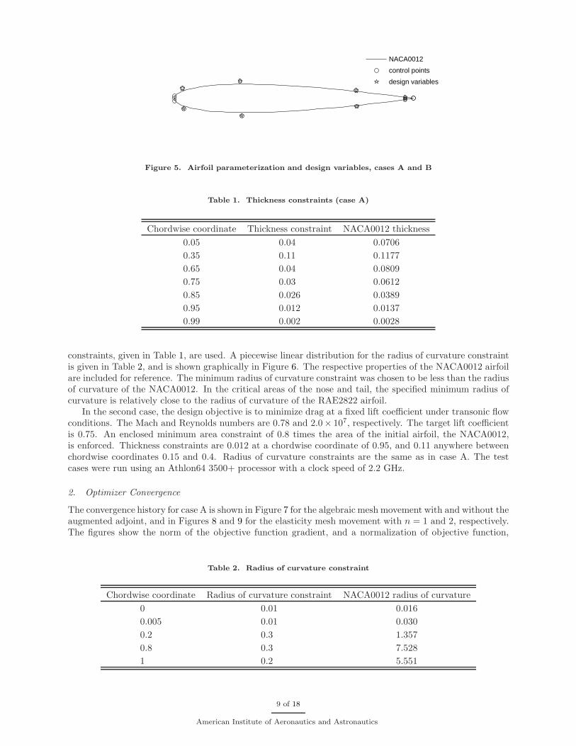
Despite the fact that the convergence histories are different when using the original and augmentedadjoint methods, they result in very similar optimized airfoils. The largest vertical displacement between theoptimized airfoils is less than 10−6 chords, when the algebraic grid perturbation is used. For the elasticitygrid perturbation, the difference is less than 10−3 chords; this is expected, given the loose convergenceobtained with the original adjoint method.

The optimized airfoils found using the augmented adjoint method, for case A, are shown in Figure 10.While the optimal airfoil shape does not depend much on the gradient calculation method, the figure showsthat the shape is dependent on the grid perturbation technique used. The two variants of the elasticity givevery similar results, but the algebraic method gives a somewhat different shape.

To explore this, a new mesh was regenerated for each of the optimized airfoils, and the objective functionswere recomputed on the new meshes. These objective functions include the constraint penalties; to maintainconsistency, the penalties are not recomputed on the regenerated mesh, but are retained from the optimizedresult. These values, given in Table 3, show that the elasticity method with n = 2 provides the shapehaving the best performance, as computed on the regenerated mesh. Also, the comparison between theresult computed on the perturbed and regenerated meshes is best for the elasticity method with n = 2, andworst for the algebraic method. This suggests that the mesh obtained using the elasticity method with n = 2has the highest quality, i.e. it is most similar to the original mesh.

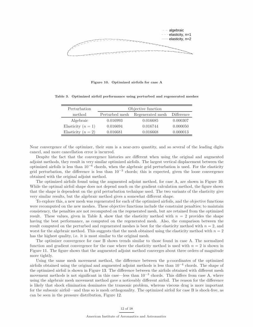
The optimizer convergence for case B shows trends similar to those found in case A. The normalizedfunction and gradient convergence for the case where the elasticity method is used with n = 2 is shown inFigure 11. The figure shows that the augmented adjoint method converges about three orders of magnitudemore tightly.

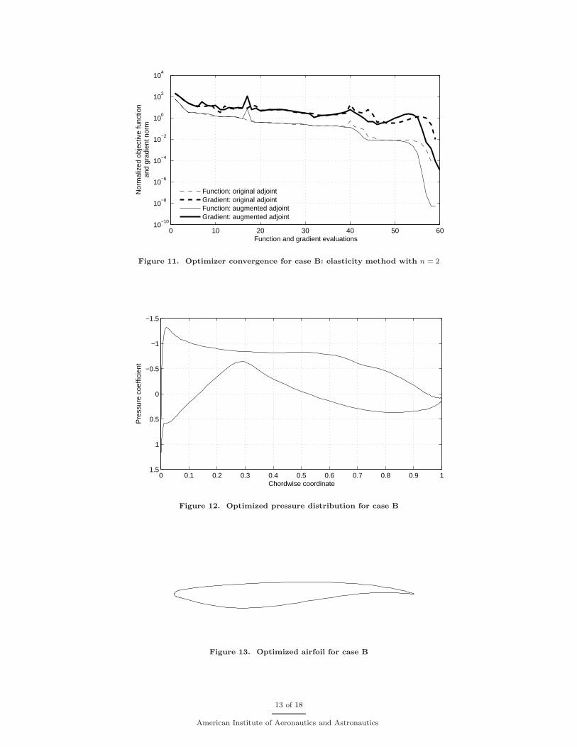
Using the same mesh movement method, the difference between the y-coordinates of the optimizedairfoils obtained using the original and augmented adjoint methods is less than 10−4 chords. The shape ofthe optimized airfoil is shown in Figure 13. The difference between the airfoils obtained with different meshmovement methods is not significant in this case—less than 10−3 chords. This differs from case A, whereusing the algebraic mesh movement method gave a noticeably different airfoil. The reason for the differenceis likely that shock elimination dominates the transonic problem, whereas viscous drag is more importantfor the subsonic airfoil—and thus so is mesh orthogonality. The optimized airfoil for case B is shock-free, ascan be seen in the pressure distribution, Figure 12.

12 of 18


0 10 20 30 40 50 6010

−10

10−8

10−6

10−4

10−2

100

102

104


Nor

mal

ized

obj

ectiv

e fu

nctio

nan

d gr

adie

nt n

orm


Figure 11. Optimizer convergence for case B: elasticity method with n = 2

0 0.1 0.2 0.3 0.4 0.5 0.6 0.7 0.8 0.9 1

−1.5

−1

−0.5

0

0.5

1

1.5

Chordwise coordinate

Pre

ssur

e co

effic

ient

Figure 12. Optimized pressure distribution for case B

Figure 13. Optimized airfoil for case B

13 of 18


0 5 10 15 20 25 30 350

5

10

15

20

25

30

35

Number of B−spline design variables

Gra

dien

t cal

cula

tion

time

[s]

Augmented adjointOriginal adjoint

Figure 14. Gradient calculation time: algebraic method, case A

0 5 10 15 20 25 30 350

100

200

300

400

500

600

700

800

900


Gra

dien

t cal

cula

tion

time

[s]


Figure 15. Gradient calculation time: elasticity method with n = 1, case A

3. Gradient Evaluation Time

The CPU time required to evaluate the gradient was investigated, considering different mesh movementtechniques, gradient evaluation methods, and numbers of design variables. In each of Figures 14–16, thegradient evaluation time for the second iteration in case A is plotted against the number of B-spline designvariables, and the augmented adjoint method is contrasted with the original adjoint method. In Figure 14,algebraic mesh movement is used. This shows little difference between the two gradient evaluation techniques,although the original method is slightly slower. This difference is indicative of the speed of the analyticcalculation of ∂R/∂G. The time taken by the augmented method actually decreases some with an increasingnumber of design variables; this is likely noise due to slightly different convergence of the solvers.

Figures 15 and 16 use the elasticity mesh movement method, with the number of increments, n, being 1and 2, respectively. The time taken by the augmented method varies by less than 5% with differing numbersof design variables, and does not show an increasing trend. Additionally, the augmented adjoint method isseveral times faster than the original adjoint method, whose time requirements increase linearly with thenumber of design variables. The evaluation time for the original adjoint method is several times longer thanthat of a flow solve (near 50 seconds).

In an entire optimization, the gradient evaluation time is essentially constant, despite warm-starting eachλ(i). This is shown in Figure 17, for case A with 8 design variables, using the elasticity grid perturbation

14 of 18


0 5 10 15 20 25 30 350

200

400

600

800

1000

1200

1400

1600


Gra

dien

t cal

cula

tion

time

[s]


Figure 16. Gradient calculation time: elasticity method with n = 2, case A

0 5 10 15 20 25 30 35 40 45 500

10

20

30

40

50

60

70

80

90

100

110

Optimizer iteration

Eva

luat

ion

time

[s]

Function

Gradient

Figure 17. Change in evaluation times during optimization

with n = 2. The figure also shows that the function evaluation (grid perturbation plus flow solution) growsincreasingly faster as the optimization progresses. This is due to warm-starting; the flow solve graduallybecomes faster, while the mesh movement accelerates abruptly near the end of the optimization. The gradientcalculation initially requires about 80% as much time as the function evaluation.

V. Conclusions

We have presented a mesh movement technique that models the mesh through the equations of linearelasticity. In order to maintain mesh quality, cells are stiffened in inverse proportion to their area andquality. Multiple mesh movement increments can be used so that the stiffening can be adjusted basedon intermediate quality measures. This mesh movement approach requires more computation than simplertechniques, such as algebraic methods, but is very robust, producing high quality meshes even for large shapechanges. An augmented adjoint approach is used to calculate adjoint variables associated with the meshmovement algorithm. Adjoint variables are computed for each increment used. The use of the augmentedadjoint method allows the optimizer to converge much more tightly than was possible using the originaladjoint method. This is indicative of increased gradient accuracy. The augmented adjoint method has a runtime that is independent of the number of design variables. With the augmented adjoint approach, the cost

15 of 18


0 5 10 15 20 25 30 350

5

10

15

20

25


Gra

dien

t cal

cula

tion

time

[s]


Figure 18. Gradient calculation time: algebraic method, case B

0 5 10 15 20 25 30 350

100

200

300

400

500

600

700

800


Gra

dien

t cal

cula

tion

time

[s]


Figure 19. Gradient calculation time: elasticity method with n = 1, case B

0 5 10 15 20 25 30 350

500

1000

1500


Gra

dien

t cal

cula

tion

time

[s]


Figure 20. Gradient calculation time: elasticity method with n = 2, case B

16 of 18


of computing the gradient is about 70–80% of that of a function evaluation (grid movement plus flow solve).

Acknowledgments

This work was sponsored by the Natural Sciences and Engineering Research Council of Canada, theCanada Research Chairs Program, Bombardier Aerospace, the Society of Naval Architects and MarineEngineers, and the University of Toronto. Their financial support is gratefully acknowledged.

References

1Farhat, C., Degand, C., Koobus, B., and Lesoinne, M., “Torsional Springs for Two-Dimensional Dynamic UnstructuredFluid Meshes”, Computer Methods in Applied Mechanics and Engineering, Vol. 163, 1998, pp. 231–245.

2Allen, C. B., “An Unsteady Flow Solver with Algebraic Grid Motion for Aeroelastic Simulations”, International Councilof the Aeronautical Sciences, ICAS 2002, Bristol, U.K., 2002. URL=http://lu.fme.vutbr.cz/icas2002/PAPERS/R3.PDF.

3Bar-Yoseph, P. Z.,Mereu, S., Chippada S., and Kalro, V. K., “Automatic Monitoring of Element Shape Quality in 2-D and 3-D Computational Mesh Dynamics”, Computational Mechanics, Vol. 27, No. 5, May 2001, pp. 378–395. URL =http://dx.doi.org/10.1007/s004660100250

4Samareh, J. A., Application of Quaternions for Mesh Deformation, NASA TM–2002–211646, Apr. 2002. URL =http://hdl.handle.net/2002/14780.

5Martineau, D. G. and Georgala, J. M., “A Mesh Movement Algorithm for High Quality Generalised Meshes”, 42nd AIAA

Fluid Dynamics Conference and Exhibit, AIAA Paper 2004–0614, Reno, NV, Jan. 2004.6Nemec, M., and Zingg, D. W., “Newton-Krylov Algorithm for Aerodynamic Design Using the Navier-Stokes Equations”,

AIAA Journal, Vol. 40, No. 6, 2002, pp. 856–859.7Nemec, M., “Optimal Shape Design of Aerodynamic Configurations: A Newton-Krylov Approach”, Ph.D Thesis, Univer-

sity of Toronto, 2003. URL = http://oddjob.utias.utoronto.ca/marian/8Nemec, M., Zingg, D. W., and Pulliam, T., “MultiPoint and Multi-Objective Aerodynamic Shape Optimization”, AIAA

Journal, Vol. 42, No. 6, Jun. 2004, pp. 1057–1065.9Burgreen, G. W., Baysal, O., and Eleshaky, M. E., “Improving the Efficiency of Aerodynamic Shape Optimization”, AIAA

Journal, Vol. 32, No. 1, 1994, pp.69–76.10Burgreen, G. W. and Baysal, O., “Three-Dimensional Aerodynamic Shape Optimization Using Discrete Sensitivity Anal-

ysis”, AIAA Journal, Vol. 34, No. 9, 1996, pp. 1761–1770.11Jones, W. T., and Samareh, J. A., “A Grid Generation System for Multidisciplinary Design Optimization”, Proceedings

of the AIAA 12th Computational Fluid Dynamics Conference, AIAA Paper 1995–1689, Washington, DC,12Degand, C. and Farhat, C., “A Three-Dimensional Torsional Spring Analogy Method for Unstructured Dynamic Meshes”,

Computers and Structures, Vol. 80, 2002, pp. 305–316. URL=http://hdl.handle.net/2002/1541013Stein, K., Tezduyar, T., and Benney, R., “Mesh Moving Techniques for Fluid-Structure Interactions with Large Displace-

ments”, Journal of Applied Mechanics, Vol. 70, No. 1, Jan 2003, pp. 58–63.14, Neilson, E. J. and Anderson, W. K., “Recent Improvements in Aerodynamic Design Optimization on Unstructured

Meshes”, AIAA Journal, Vol. 40, No. 6, June 2002, pp. 1155–1163.15Tezduyar, T. E., Behr, M., Mittal, S., and Johnson, A. A., “Computation of Unsteady Incompressible Flows with the

Stabilized Finite Element Methods: Space-time Formulations, Iterative Strategies and Massively Parallel Implementations”,New methods in Transient Analysis, Presented at the Winter Annual Meeting of the American Society of Mechanical Engineers,ASME, Anaheim, CA, Nov. 1992.

16Squire, W. and Trapp, G., “Using Complex Variables to Estimate Derivatives of Real Functions”, SIAM Review, Vol. 40,No. 1, Mar. 1998, pp. 110–112

17Martins, J. R. R. A., Sturdza, P., and Alonso J. J., “The Complex-Step Derivative Approximation”, ACM Transactions

on Mathematical Software, Vol. 29, No. 3, Sep. 2003, pp. 245–262. URL=http://doi.acm.org/10.1145/838250.83825118Griewank,A., Evaluating Derivatives: Principles and Techniques of Algorithmic Differentiation, Society for Industrial

and Applied Mathematics, Philadelphia, 2000.19Pironneau, O., “On Optimum Design in Fluid Mechanics”, Journal of Fluid Mechanics, Vol. 64, 1974, pp. 97–110.20Jameson, A., “Aerodynamic Design via Control Theory”, Journal of Scientific Computing, Vol. 3, No. 3, 1988, pp.

233–260.21Anderson, W. K. and Venkatakrishnan, V., “Aerodynamic Design Optimization on Unstructured Grids with a Continuous

Adjoint Formulation”, Computers & Fluids, Vol. 28, 1999, pp. 443–480.22Kim, H. and Nakahashi, K., “Flap-Deflection Optimization for Transonic Cruise Performance Improvement of Supersonic

Transport Wing”, Journal of Aircraft, Vol. 38, No. 4, 2001, pp. 709–717.23Kim, H., Obayashi, S., and Nakahashi, K., “Aerodynamic Optimization of Supersonic Transport Wing Using Unstructured

Adjoint Method”, AIAA Journal, Vol. 39, No. 6, 2001, pp. 1011–1020.24Martins, J. R. R. A., Alonso J. J., and Reuther J. J., “A Coupled-Adjoint Sensitivity Analysis Method for

High-Fidelity Aero-Structural Design”, Optimization and Engineering, Vol. 6, No. 1, Mar. 2005, pp. 33–62. URL =http://www.kluweronline.com/issn/1389-4420/contents.

25Le Moigne, A. and Qin, N., “Variable-Fidelity Aerodynamic Optimization for Turbulent Flows Using a Discrete AdjointFormulation”, AIAA Journal, Vol. 42, No. 7, 2004, pp. 1281–1292.

17 of 18


26Bischof, C. H., Mauer, A., Jones, W. T., and Samareh, J., “Experiences with Automatic Differentiation Applied to aVolume Grid Generation Code”, Journal of Aircraft, Vol. 35, No. 4, 1998, pp. 569–573.

27Samareh, J. A., “Survey of Shape Parameterization Techniques for High-Fidelity Multidisciplinary Shape Optimization”,AIAA Journal, Vol. 39, No. 5, 2001, pp. 877–884.

28Samareh, J. A., “Novel Multidisciplinary Shape Parameterization Approach”, Journal of Aircraft, Vol. 38, No. 6, 2001,pp. 1015–1024.

29Maute, K., Nikbay, M., and Farhat, C., “Sensitivity Analysis and Design Optimization of Three-Dimensional Non-LinearAeroelastic Systems by the Adjoint Method”, International Journal for Numerical Methods in Engineering, Vol. 56, No. 6,Feb. 2003, pp. 911–933.

30Nielsen, E. J. and Park, M. A., “Using an Adjoint Approach to Eliminate Mesh Sensitivities in Computational Design”,AIAA Journal, Vol. 44, No. 5, May 2006, pp. 948–953.

31Dimitri J. M., “Multigrid Solution of the Discrete Adjoint for Optimization Problems on Unstructured Meshes”, AIAA

Journal, Vol. 44, No. 1, Jan. 2006.32Sadrehaghighi, I., Smith, R. E., and Twari, S. N., “Grid Sensitivity and Aerodynamic Optimization of Generic Airfoils”,

Journal of Aircraft, Vol. 32, No. 6, 1995, pp. 1234–1239.33Korivi, V. M., Newman, P. A., and Taylor, III, A. C., “Aerodynamic Optimization Using Sensitivity Derivatives From a

Three-dimensional Supersonic Euler code”, Journal of Aircraft, Vol. 35. No. 3, 1998, pp. 405–411.34Barger, R. L., Adams, M. S., and Krishnan, R. R., “Automatic Computation of Euler Marching Grids and Subsonic

Grids for Wing-Fuselage Configurations”, NASA TM 4573, Jul. 1994.35Pagaldipti, N. and Chattopadhyay, A., “A Discrete Semianalytical Procedure for Aerodynamic Sensitivity Analysis

Including Grid Sensitivity”, Computers & Mathematics with Applications, Vol. 32, No. 3, 1996, pp. 61–71.36Gunzburger, M., “Introduction to the Mathematical Aspects of Flow Control and Optimisation”, Inverse Design and

Optimisation Methods, von Karman Institute of Fluid Dynamics, Brussels, Belgium, Apr. 1997.37Chattopadhyay, A. and Pagaldipti, N., “Multidisciplinary Optimization Using Semi-analytical Sensitivity Analysis Pro-

cedure and Multilevel Decomposition”, Computers & Mathematics with Applications, Vol. 29, No. 7, Apr. 1995.38Dongarra, J., Lumsdaine, A., Pozo, R., and Remington, K., “A Sparse Matrix Library in C++ for High Per-

formance Architectures”, Proceedings of the Second Object Oriented Numerics Conference, 1992, pp. 214–218. URL =ftp://math.nist.gov/pub/pozo/papers/sparse.ps.Z.

18 of 18


Documents

Mesh Movement for a Discrete-Adjoint Newton-Krylov Algorithm for