Embed Size (px)
Citation preview
MESH-FREE METHODS FOR HEAT TRANSFER AND FLUID FLOW
Boidar arlerLaboratory for Multiphase Processes
Nova Gorica Polytechnic, Nova Gorica, Slovenia
Institut Podstawowych Problemov TechnikiPolska Akademia NaukCentrum Doskonalosci
Nowoczesne Materialy i KonstrukcjeWarszawa, Polska, kwiecien 14, 2003
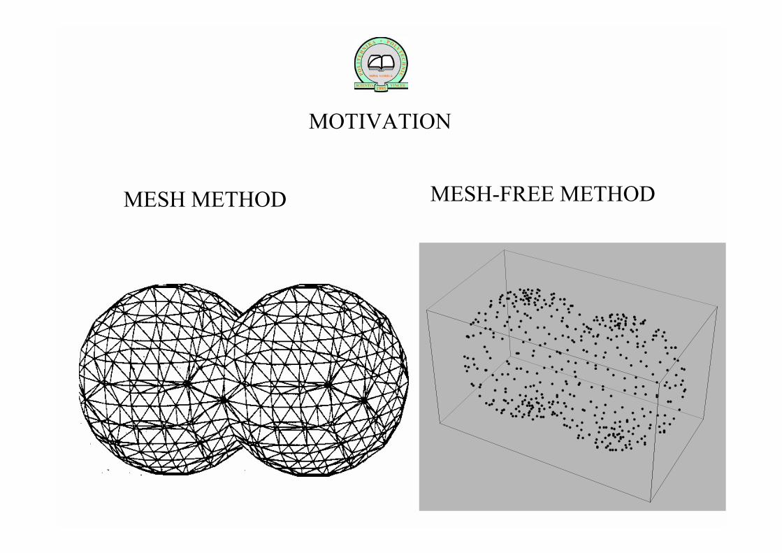
MESH METHOD MESH-FREE METHOD
MOTIVATION

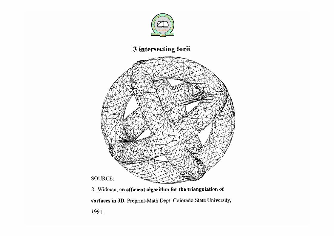
BASIC LITERATURE
S.N. Atluri, S. Shen, The Meshless Method, Tech Science Press, Los Angeles, 2002.
G.R. Liu, Mesh Free Methods, CRC Press, Boca Raton, 2003.
NEW COMPUTATIONAL DISCIPLINE
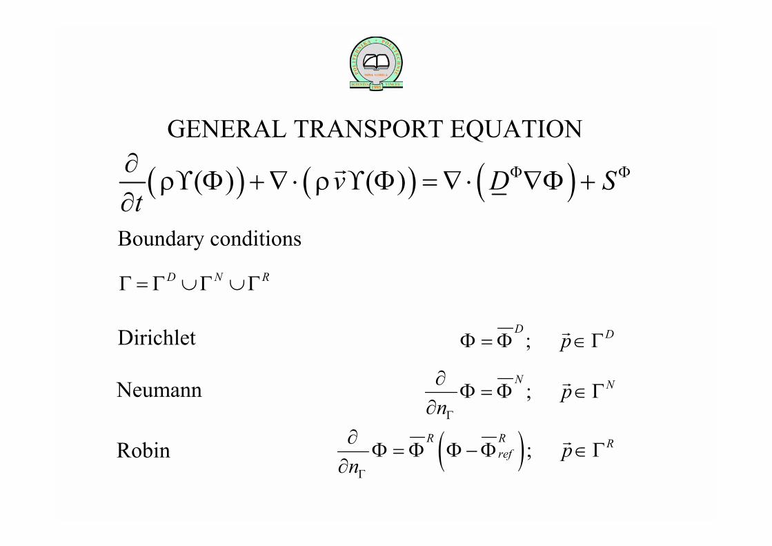
GENERAL TRANSPORT EQUATION
( ) ( ) ( )( ) ( )v D Stρ ρ Φ Φ∂ϒ Φ +∇ ⋅ ϒ Φ = ∇ ⋅ ∇Φ +
∂r
Boundary conditionsRND Γ∪Γ∪Γ=Γ
;D DpΦ = Φ ∈Γ
r
;N Np
nΓ
∂Φ = Φ ∈Γ
∂r
( );R R Rref p
nΓ
∂Φ = Φ Φ −Φ ∈Γ
∂r
Dirichlet
Neumann
Robin
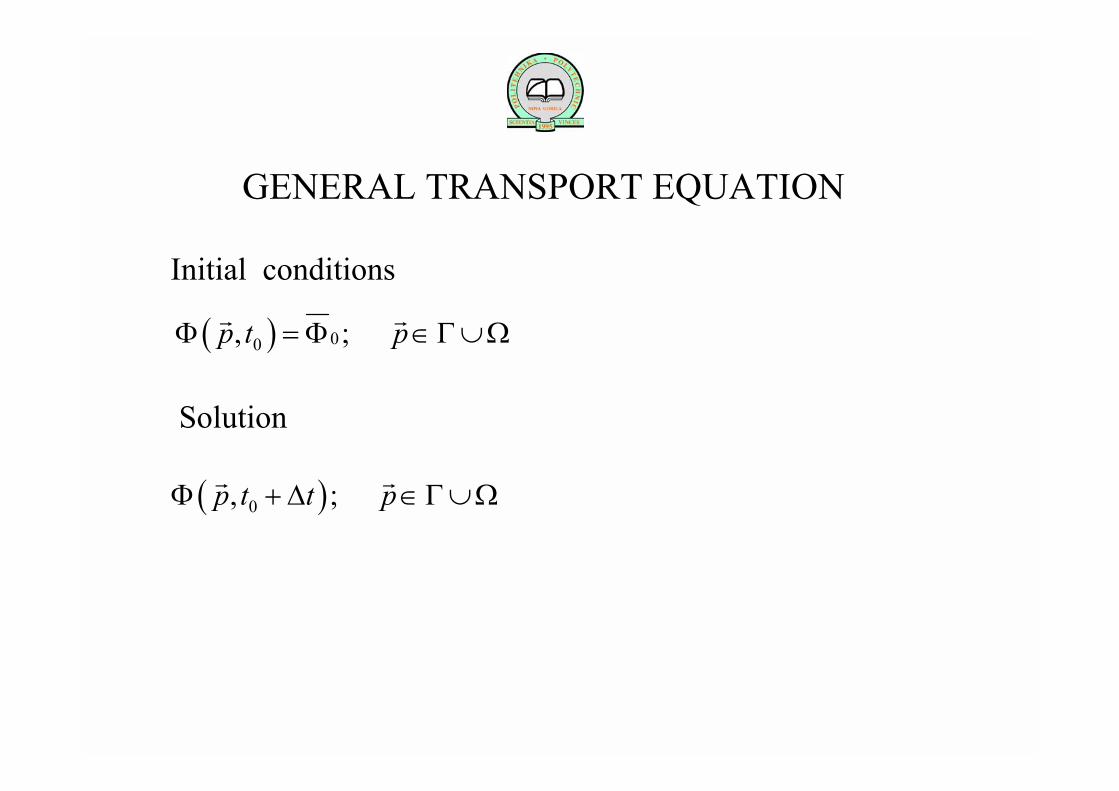
GENERAL TRANSPORT EQUATION
Initial conditions
( ) 00, ;p t pΦ = Φ ∈Γ∪Ωr r
Solution
( )0, ;p t t pΦ +∆ ∈Γ∪Ωr r

DIFFUSION TENSOR
11 12 13
21 22 23
31 32 33
d d dD d d d
d d d
Φ
=
1 0 00 1 00 0 1
I =
'D D I DΦ Φ Φ= +
11 12 13
21 22 23
31 32 33
'd D d d
D d d D dd d d D
Φ
Φ Φ
Φ
−
= − −
Splitting
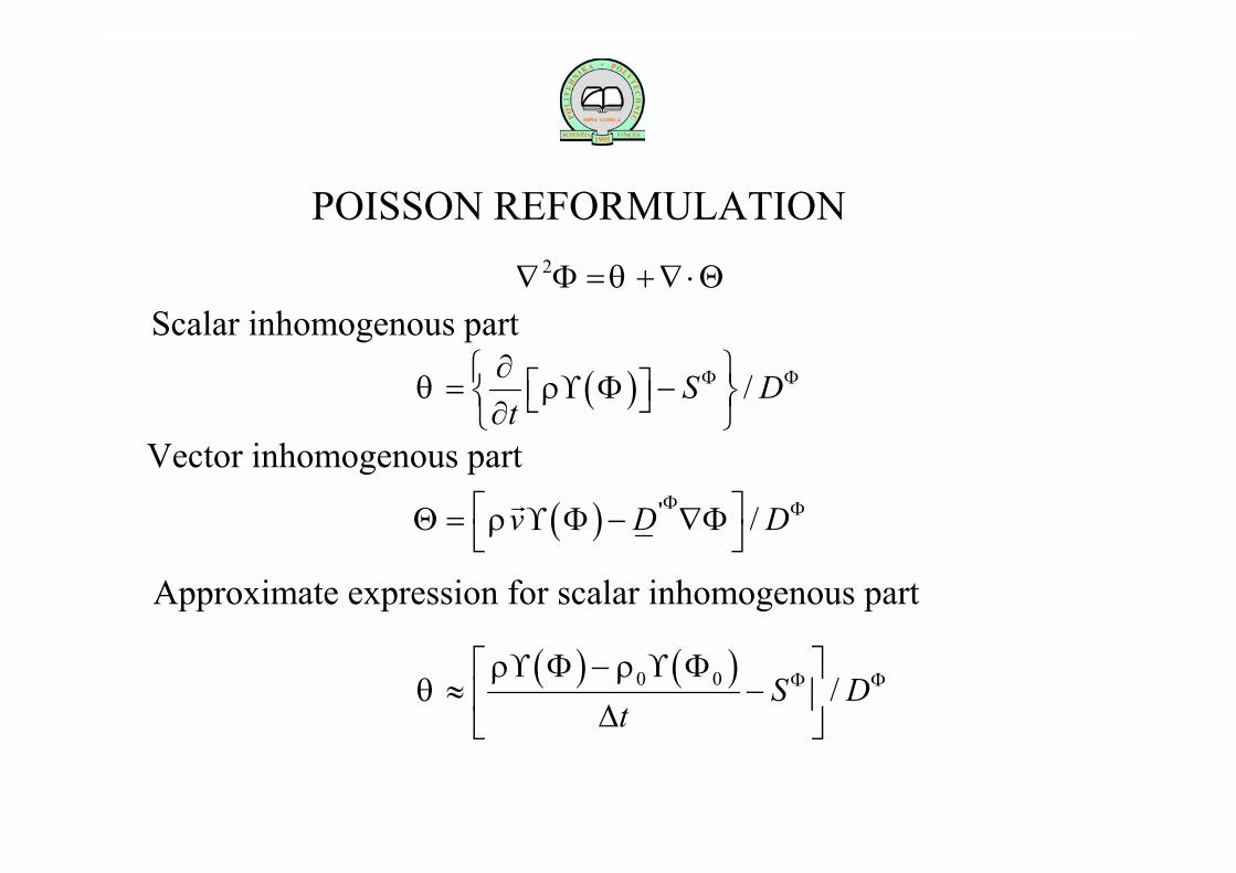
POISSON REFORMULATION
Θ⋅∇+=Φ∇ θ2
( ) /S Dt
θ ρ Φ Φ∂ = ϒ Φ − ∂
( ) /v D DρΦ Φ = ϒ Φ − ∇Φ
'rΘ
( ) ( )0 0 /S Dt
ρ ρθ Φ Φ ϒ Φ − ϒ Φ≈ − ∆
Approximate expression for scalar inhomogenous part
Scalar inhomogenous part
Vector inhomogenous part

TAYLOR EXPANSION
( )Φ−Φ+≈ Φ,θθθ
( ) ( )Φ−Φ⋅∇+⋅∇+Φ−Φ+=⋅∇+=Φ∇ ΦΦ ,,2 ΘΘΘ θθθ
( )Φ−Φ+≈ Φ,ΘΘΘ
Final Poisson form

ITERATION STRATEGIES
Nonlinear
Highly non-linear
2 1j j jθ+∇ Φ = +∇ ⋅Θ
( ) ( )2, ,
1 1 1j jj jj j jθ θ Φ+ + +
Φ∇ = + −Φ +∇Φ Φ Φ⋅ +∇⋅ −ΦΘ Θ
( )1 1j j j jrelcθ θ θ θ− −= + − ( )1 1j j j j
relc− −∇ ⋅ = ∇ ⋅ + ∇ ⋅ −∇ ⋅Θ Θ Θ Θ
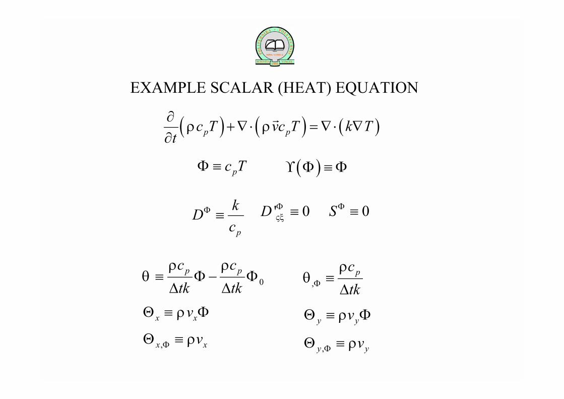
( ) ( ) ( )p pc T vc T k Ttρ ρ
∂+∇ ⋅ = ∇ ⋅ ∇
∂r
Tcp≡Φ ( )ϒ Φ ≡ Φ
p
kDc
Φ ≡ ' 0D ςξΦ ≡ 0SΦ ≡
0Φ∆
−Φ∆
≡tkc
tkc pp ρρ
θtkcp
∆≡Φ
ρθ,
x xvρΘ ≡ Φ Φ≡Θ yy vρ
xx vρ≡Θ Φ, yy vρ≡Θ Φ,
EXAMPLE SCALAR (HEAT) EQUATION
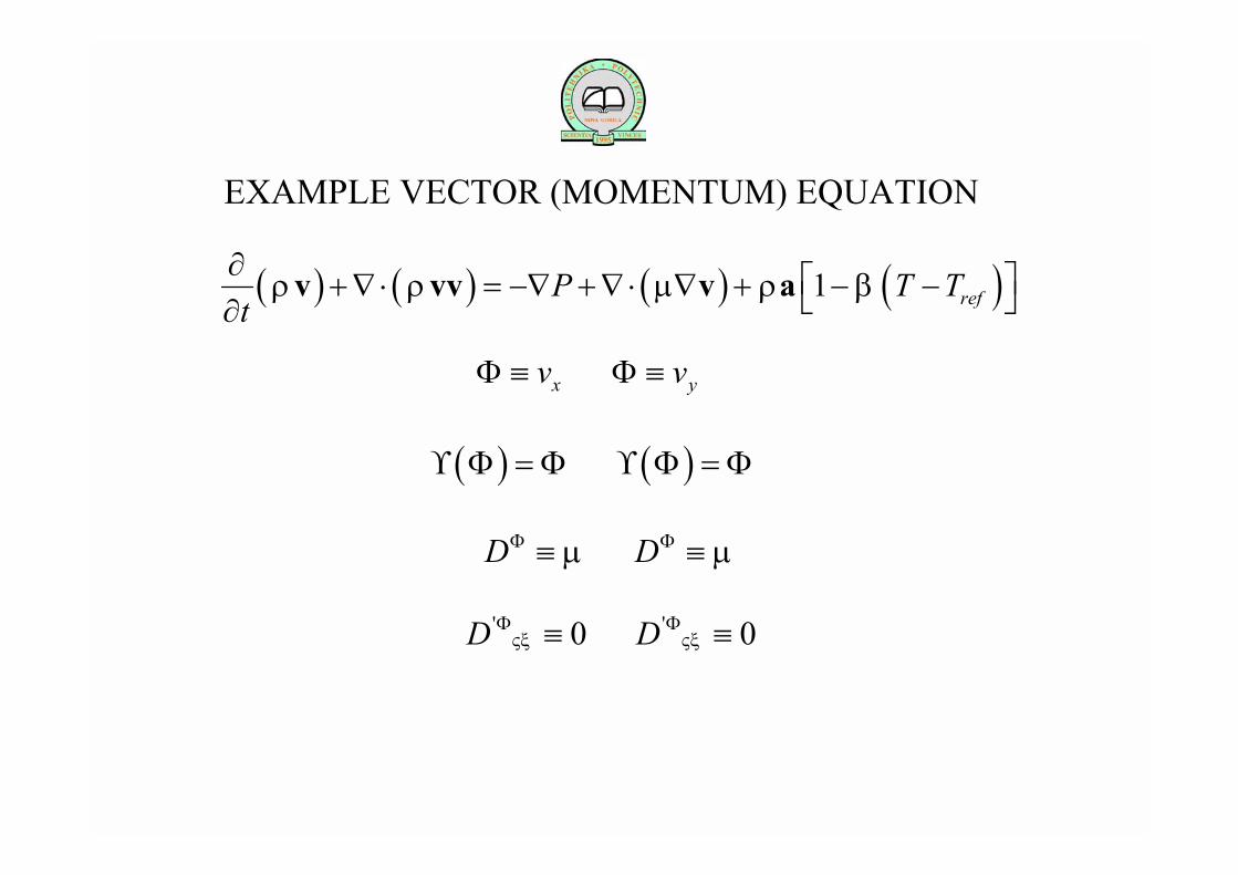
( ) ( ) ( ) ( )1 refP T Ttρ ρ µ ρ β
∂ +∇ ⋅ = −∇ +∇ ⋅ ∇ + − − ∂v vv v a
x yv vΦ ≡ Φ ≡
( ) ( )ϒ Φ = Φ ϒ Φ = Φ
D Dµ µΦ Φ≡ ≡
EXAMPLE VECTOR (MOMENTUM) EQUATION
' '0 0D Dςξ ςξΦ Φ≡ ≡
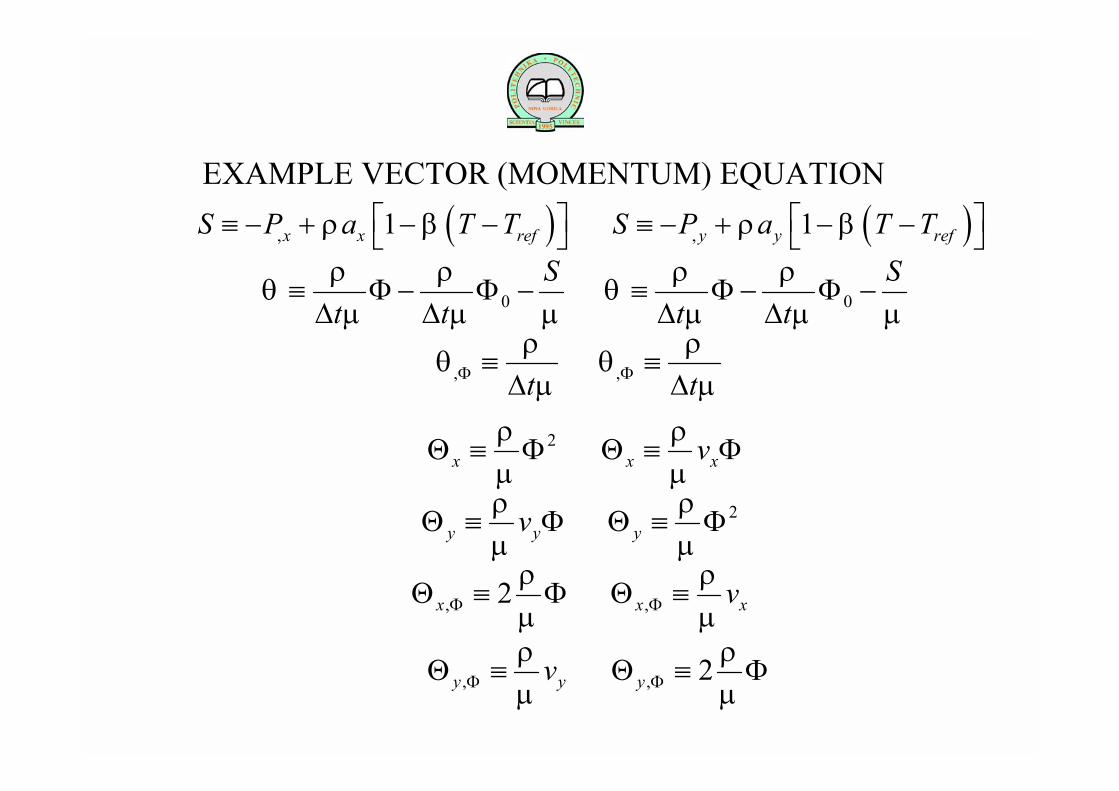
EXAMPLE VECTOR (MOMENTUM) EQUATION
( ) ( ), ,1 1x x ref y y refS P a T T S P a T Tρ β ρ β ≡ − + − − ≡ − + − −
0 0S S
t t t tρ ρ ρ ρ
θ θµ µ µ µ µ µ
≡ Φ − Φ − ≡ Φ − Φ −∆ ∆ ∆ ∆
, ,t tρ ρ
θ θµ µΦ Φ≡ ≡
∆ ∆
2x x xvρ ρ
µ µΘ ≡ Φ Θ ≡ Φ
2y y yvρ ρ
µ µΘ ≡ Φ Θ ≡ Φ
, ,2x x xvρ ρµ µΦ ΦΘ ≡ Φ Θ ≡
, , 2y y yvρ ρµ µΦ ΦΘ ≡ Θ ≡ Φ
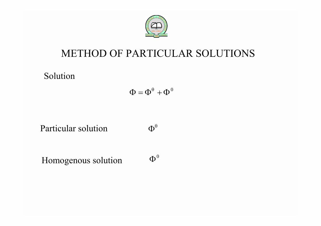
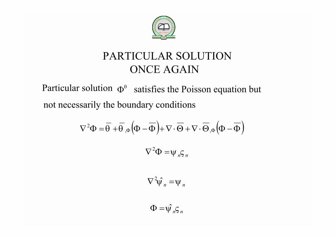
METHOD OF PARTICULAR SOLUTIONS
θΦParticular solution
0Φ+Φ=Φ θ
0ΦHomogenous solution
Solution

PARTICULAR SOLUTION θΦParticular solution satisfies the Poisson equation but
not necessarily the boundary conditions
( ) ( )2, ,
θ θ θ Φ Φ∇ Φ = + Φ −Φ +∇⋅ +∇ ⋅ Φ −ΦΘ Θ
2 θ θ∇ Φ = +∇⋅Θ

HOMOGENOUS SOLUTION
0ΦHomogenous solution satisfies the Laplace equation
with the modified boundary conditions
002 =Φ∇
0 ;N Np
n nθ
Γ Γ
∂ ∂Φ = Φ − Φ ∈Γ
∂ ∂r
( )0 ;R R R
ref pn n
θ
Γ Γ
∂ ∂Φ = Φ Φ −Φ − Φ ∈Γ
∂ ∂r
0 ;D DpθΦ = Φ −Φ ∈Γ
r
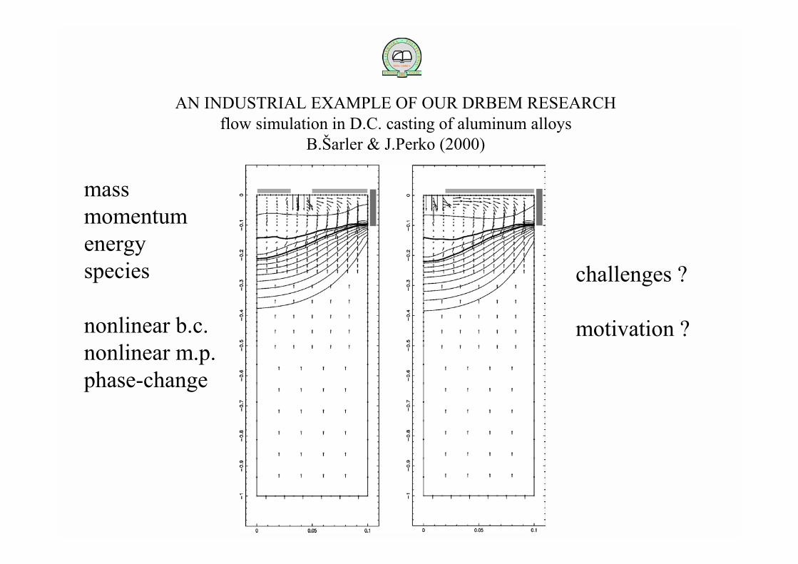
AN INDUSTRIAL EXAMPLE OF OUR DRBEM RESEARCHflow simulation in D.C. casting of aluminum alloys
B.arler & J.Perko (2000)
challenges ?
motivation ?
massmomentumenergyspecies
nonlinear b.c.nonlinear m.p.phase-change

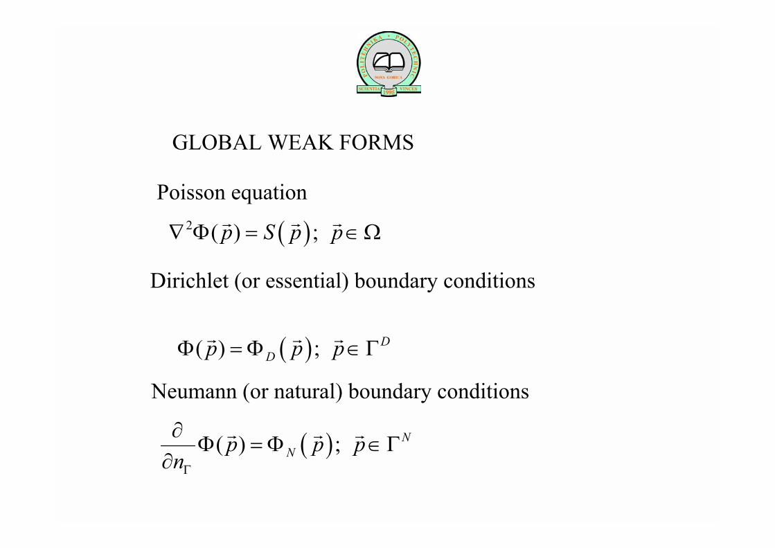
GLOBAL WEAK FORMS
( )2 ( ) ;p S p p∇ Φ = ∈Ωr r r
( )( ) ; DDp p pΦ = Φ ∈Γ
r r r
( )( ) ; NNp p p
nΓ
∂Φ = Φ ∈Γ
∂r r r
Dirichlet (or essential) boundary conditions
Neumann (or natural) boundary conditions
Poisson equation
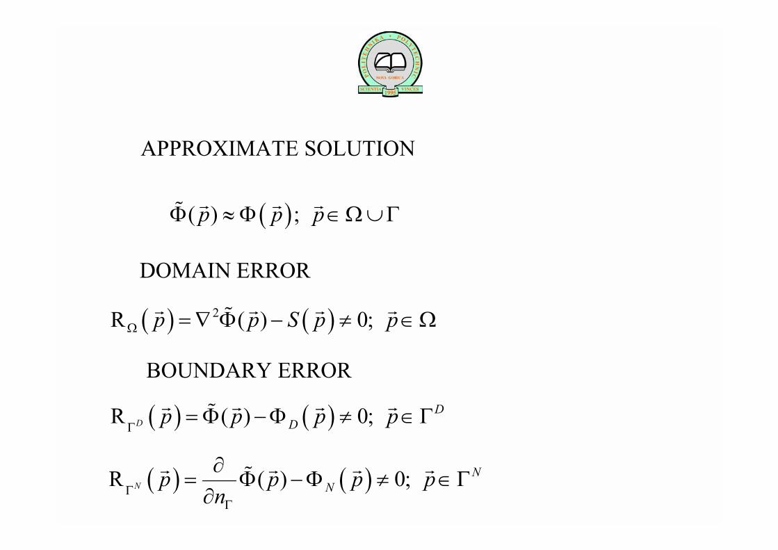
( )( ) ;p p pΦ ≈ Φ ∈Ω∪Γr r r%
DOMAIN ERROR
BOUNDARY ERROR
( ) ( )2 ( ) 0;p p S p pΩ = ∇ Φ − ≠ ∈Ωr r r r%R
APPROXIMATE SOLUTION
( ) ( )( ) 0;DD
Dp p p pΓ
= Φ −Φ ≠ ∈Γr r r r%R
( ) ( )( ) 0;NN
Np p p pnΓΓ
∂= Φ −Φ ≠ ∈Γ∂
r r r r%R

CONCEPT OF TRIAL FUNCTION
BEST SOLUTION
1( ) ( )
N
n nn
p c pψ=
Φ =∑r r%
Nullification of errors ΩR ΓRand in some fashion
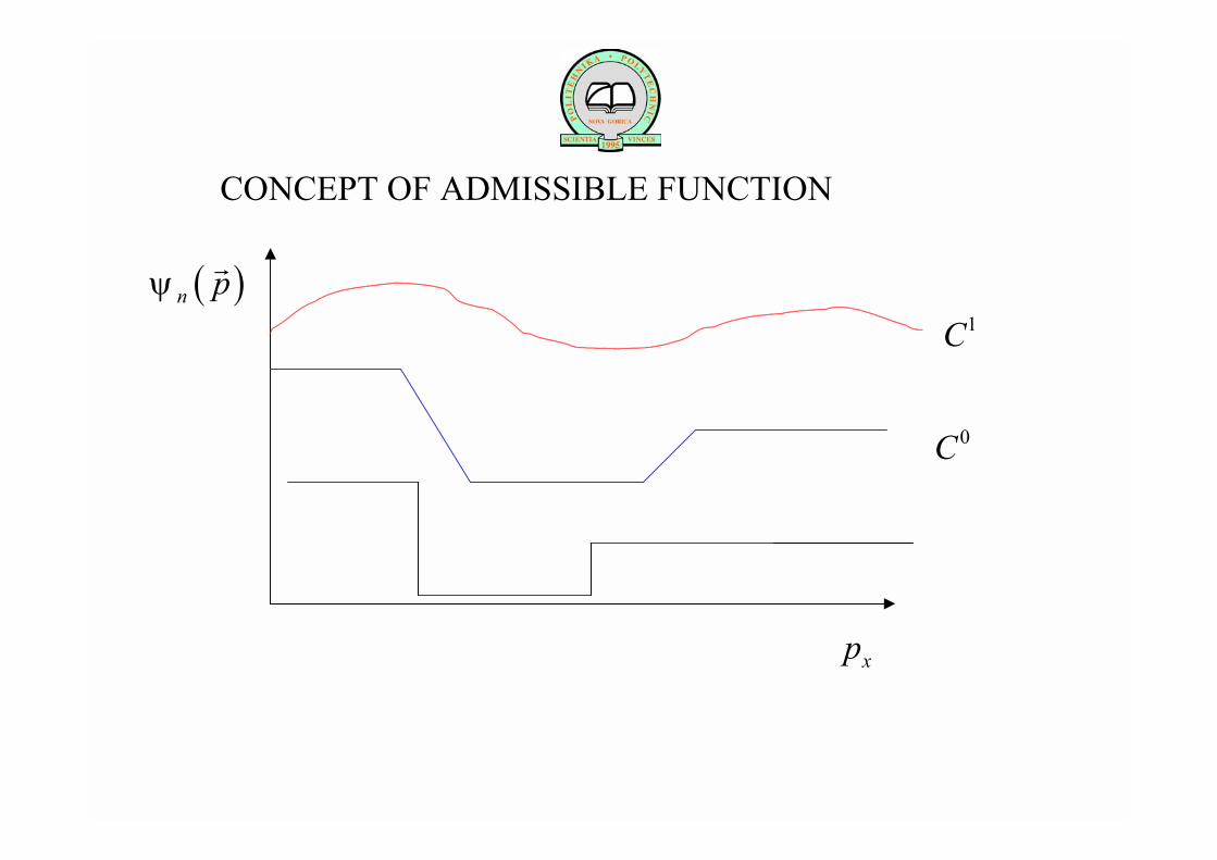
CONCEPT OF ADMISSIBLE FUNCTION
Trial function should satisfy minimum requirements
0C 1C continuous, for example
( )n pψr
CONCEPT OF ADMISSIBLE FUNCTION
0C
1C( )n pψr
xp
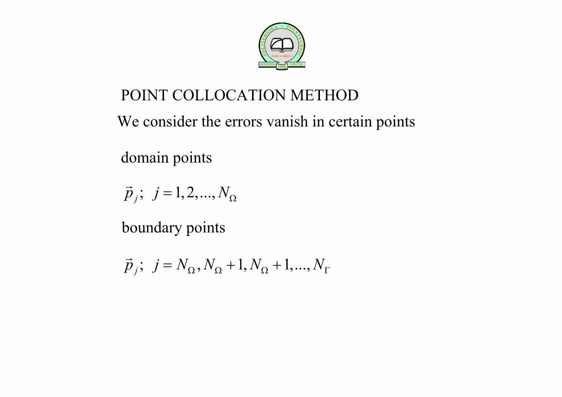
POINT COLLOCATION METHODWe consider the errors vanish in certain points
; 1,2,...,jp j NΩ=r
; , 1, 1,...,jp j N N N NΩ Ω Ω Γ= + +r
domain points
boundary points
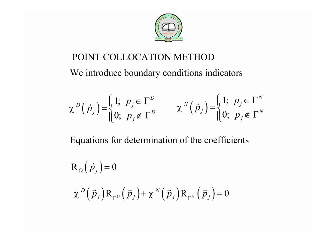
POINT COLLOCATION METHODWe introduce boundary conditions indicators
( ) 1;0;
DjD
j Dj
pp
pχ
∈Γ= ∉Γ
r ( ) 1;0;
NjN
j Nj
pp
pχ
∈Γ= ∉Γ
r
Equations for determination of the coefficients
( ) 0jpΩ =rR
( ) ( ) ( ) ( ) 0D ND N
j j j jp p p pχ χΓ Γ
+ =r r r rR R
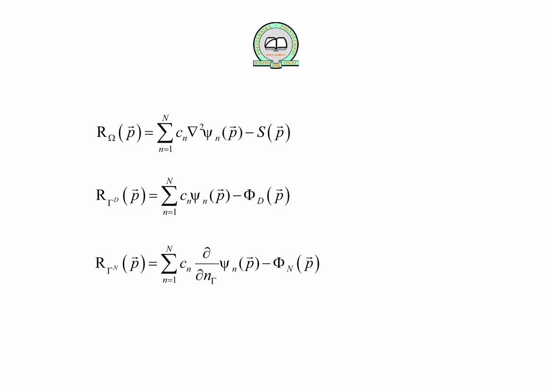
( ) ( )2
1
( )N
n nn
p c p S pψΩ=
= ∇ −∑r r rR
( ) ( )1
( )D
N
n n Dn
p c p pψΓ
=
= −Φ∑r r rR
( ) ( )1
( )N
N
n n Nn
p c p pnψ
Γ= Γ
∂= −Φ
∂∑r r rR
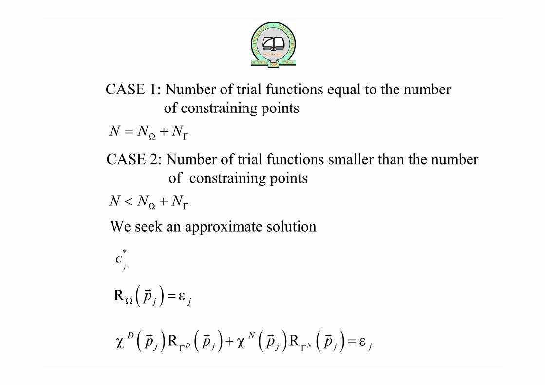
CASE 1: Number of trial functions equal to the numberof constraining points
N N NΩ Γ= +
CASE 2: Number of trial functions smaller than the numberof constraining points
N N NΩ Γ< +
We seek an approximate solution*j
c
( )j jp εΩ =rR
( ) ( ) ( ) ( )D ND N
j j j j jp p p pχ χ εΓ Γ
+ =r r r rR R
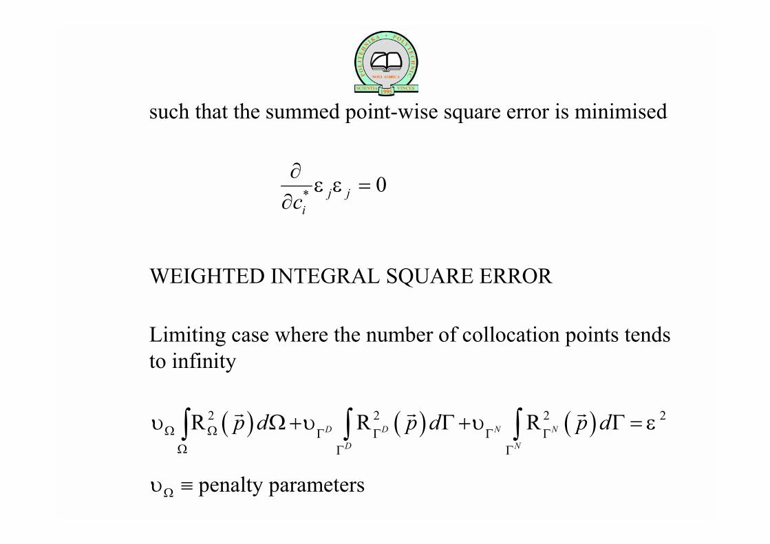
such that the summed point-wise square error is minimised
* 0j jicε ε
∂=
∂
Limiting case where the number of collocation points tendsto infinity
( ) ( ) ( )2 2 2 2D D N N
D N
p d p d p dυ υ υ εΩ Ω Γ Γ Γ ΓΩ Γ Γ
Ω+ Γ + Γ =∫ ∫ ∫r r rR R R
υΩ ≡ penalty parameters
WEIGHTED INTEGRAL SQUARE ERROR
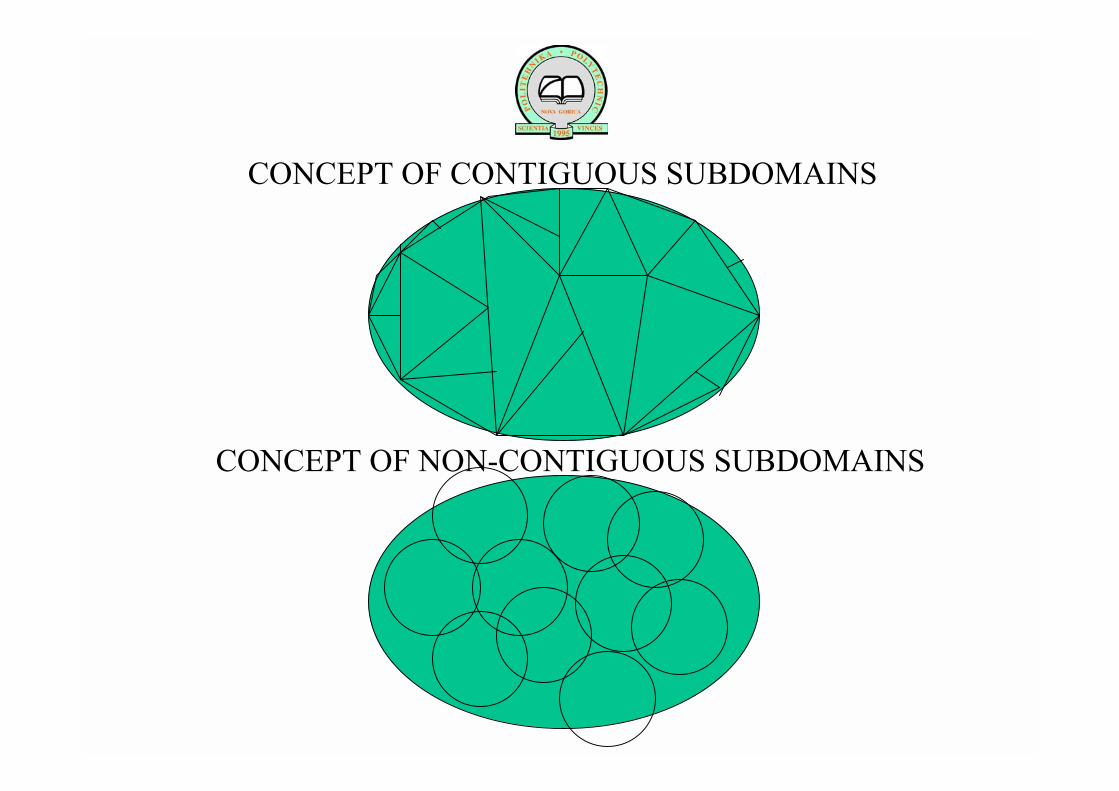
CONCEPT OF CONTIGUOUS SUBDOMAINS
CONCEPT OF NON-CONTIGUOUS SUBDOMAINS

SUBDOMAIN/AVERAGE ERROR METHODContiguous (non-overlapping) subdomains
k kΩ Γ
We may set
( ) 0jp dΩΩ
Ω =∫r
k
R
( ) ( ) ( ) ( ) 0D ND N
j j j jp p p p dχ χΓ Γ
Γ
+ Γ = ∫r r r r
k
R R
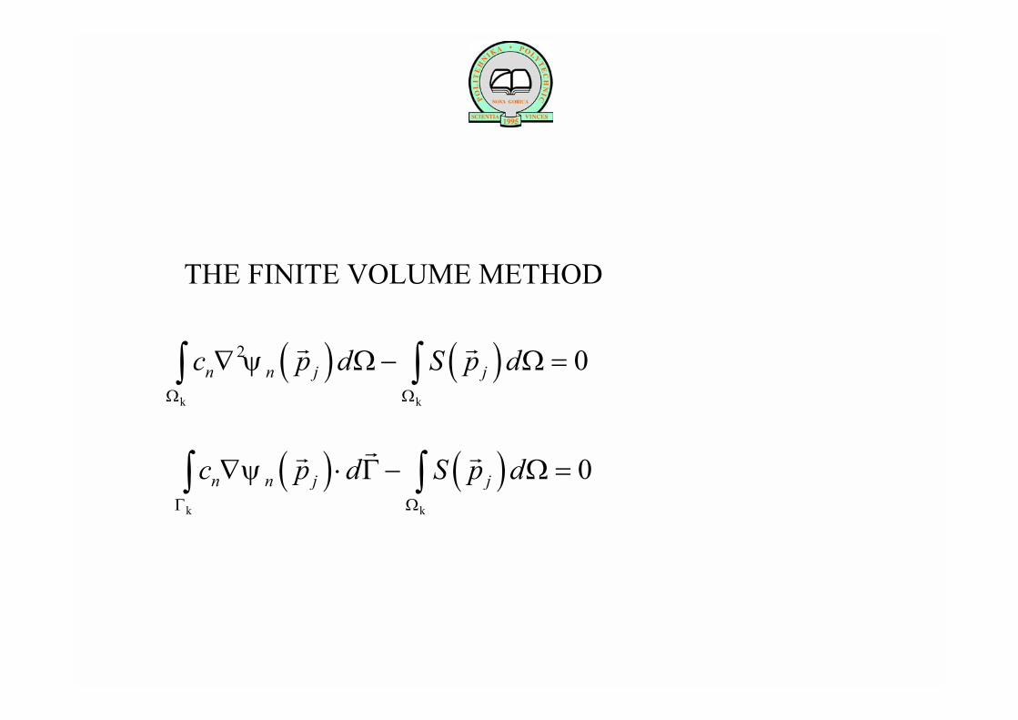
THE FINITE VOLUME METHOD
( ) ( )2 0n n j jc p d S p dψΩ Ω
∇ Ω− Ω =∫ ∫r r
k k
( ) ( ) 0n n j jc p d S p dψΓ Ω
∇ ⋅ Γ − Ω =∫ ∫rr r
k k
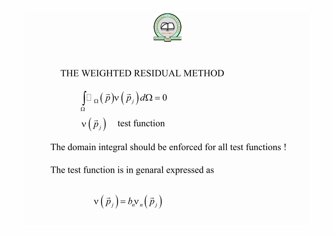
THE WEIGHTED RESIDUAL METHOD
( ) ( ) 0jp p dνΩΩ
Ω =∫r r
#
( )jpνr test function
The domain integral should be enforced for all test functions !
The test function is in genaral expressed as
( ) ( )j n n jp b pν ν=r r

SPECIAL CASES OF THE TEST FUNCTIONS
( )1;0;
k
k
pp
pν
∈Ω= ∉Ω
rr
r The Finite Volume Method
( ) ( )jp p pν δ= −r r r
The Point Collocation Method
( ) ( )p pν Ω=r r
# The Least Square Error Method

THE GLOBAL UNSYMMETRIC WEAK FORM (GUWF-I)
( ) ( ) ( )2 0j jp S p p dνΩ
∇ Φ − Ω = ∫r r r%
Requirements on
Requirements on
( ) 1: jp CΦ Φ ∈r% %
:ν none
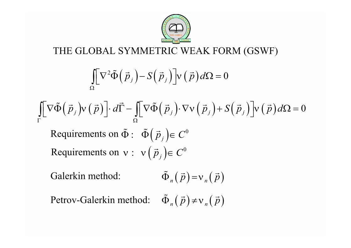
THE GLOBAL SYMMETRIC WEAK FORM (GSWF)
( ) ( ) ( )2 0j jp S p p dνΩ
∇ Φ − Ω = ∫r r r%
Requirements on
Requirements on( ) 0: jp CΦ Φ ∈r% %
( ) 0: jp Cν ν ∈r
( ) ( ) ( ) ( ) ( ) ( ) 0j j j jp p d p p S p p dν ν νΓ Ω
∇Φ ⋅ Γ − ∇Φ ⋅∇ + Ω = ∫ ∫rr r r r r r% %
Galerkin method:
Petrov-Galerkin method:
( ) ( )n np pνΦ =r r%
( ) ( )n np pνΦ ≠r r%
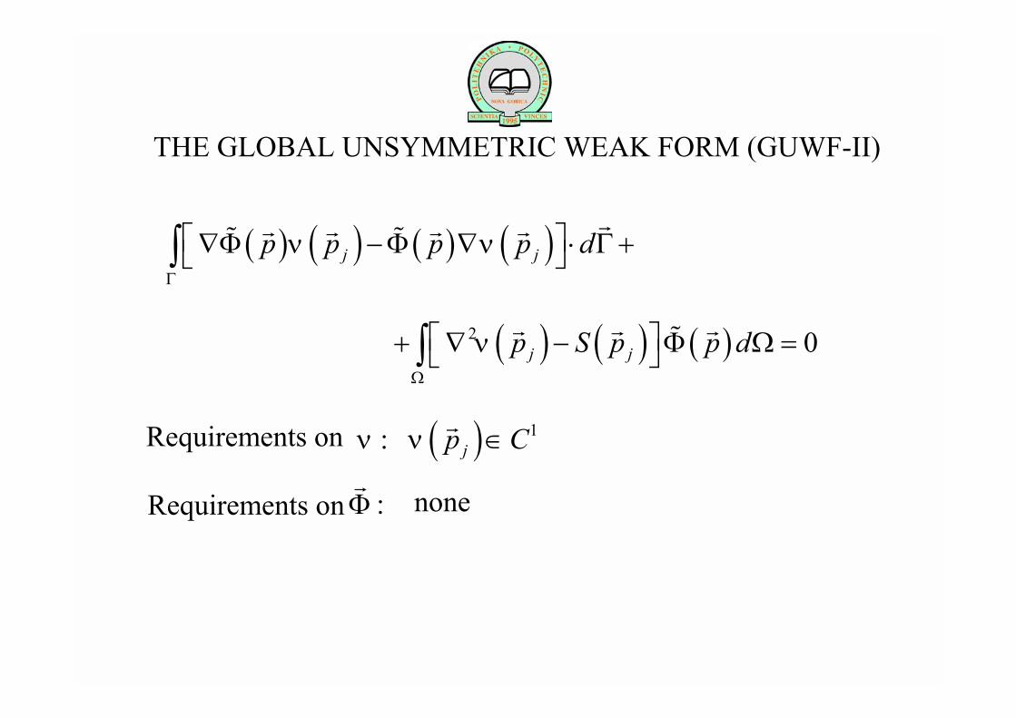
THE GLOBAL UNSYMMETRIC WEAK FORM (GUWF-II)
( ) ( ) ( ) ( )j jp p p p dν νΓ
∇Φ −Φ ∇ ⋅ Γ + ∫rr r r r% %
Requirements on
Requirements on
( ) 1: jp Cν ν ∈r
:Φr
none
( ) ( ) ( )2 0j jp S p p dνΩ
+ ∇ − Φ Ω = ∫r r r%

CONCEPT OF CONTIGUOUS SUBDOMAINS
CONCEPT OF NON-CONTIGUOUS SUBDOMAINS
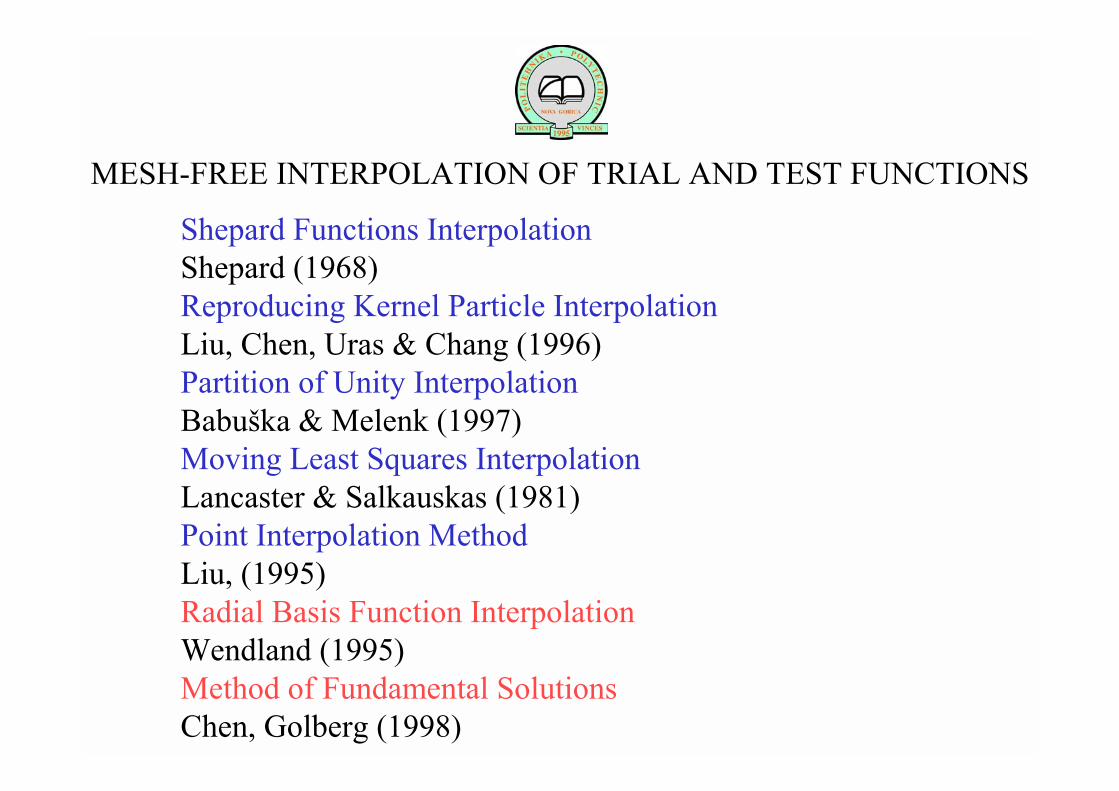
MESH-FREE INTERPOLATION OF TRIAL AND TEST FUNCTIONS
Shepard Functions InterpolationShepard (1968)Reproducing Kernel Particle InterpolationLiu, Chen, Uras & Chang (1996)Partition of Unity InterpolationBabuka & Melenk (1997)Moving Least Squares InterpolationLancaster & Salkauskas (1981)Point Interpolation MethodLiu, (1995)Radial Basis Function InterpolationWendland (1995)Method of Fundamental SolutionsChen, Golberg (1998)
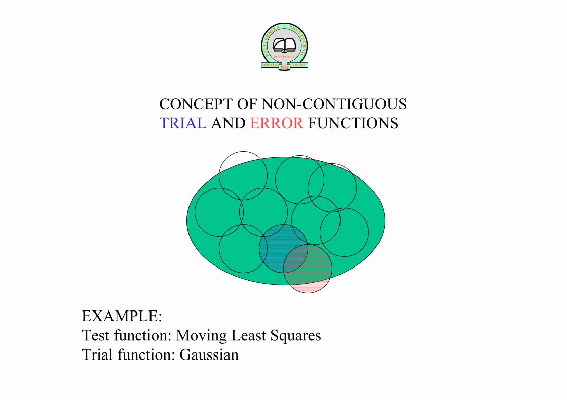
CONCEPT OF NON-CONTIGUOUS TRIAL AND ERROR FUNCTIONS
EXAMPLE:Test function: Moving Least SquaresTrial function: Gaussian
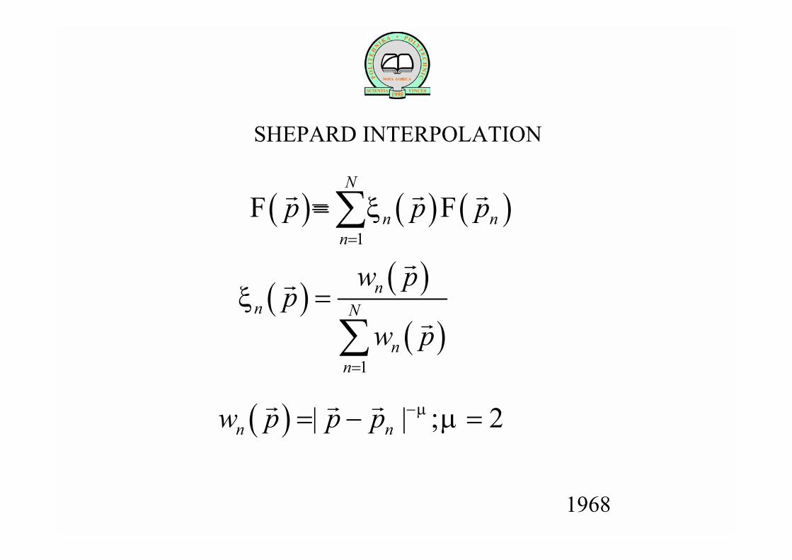
SHEPARD INTERPOLATION
( ) ( ) ( )1
N
n nn
p p pξ=
=∑r r rF = F
( ) ( )
( )1
nn N
nn
w pp
w pξ
=
=
∑
rr
r
( ) | | ; 2n nw p p p µ µ−= − =r r r
1968
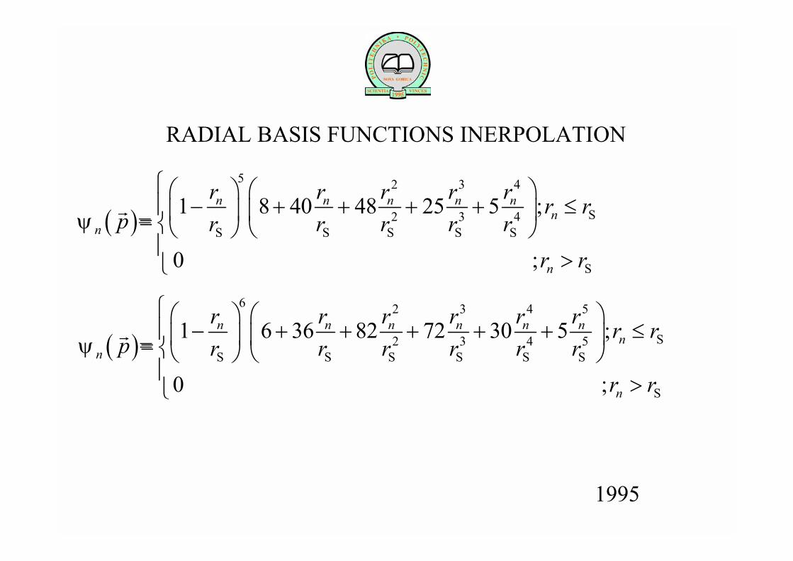
RADIAL BASIS FUNCTIONS INERPOLATION
( )
5 2 3 4
2 3 41 8 40 48 25 5 ;
0 ;
n n n n nn
n
n
r r r r r r rp r r r r r
r r
ψ
− + + + + ≤ = >
r SS S S S S
S
=
( )
6 2 3 4 5
2 3 4 51 6 36 82 72 30 5 ;
0 ;
n n n n n nn
n
n
r r r r r r r rp r r r r r r
r r
ψ
− + + + + + ≤ = >
r SS S S S S S
S
=
1995
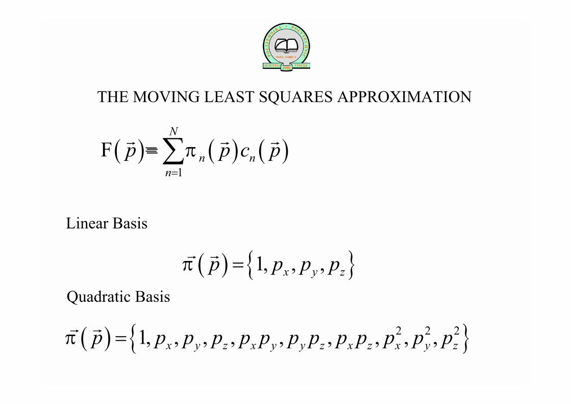
THE MOVING LEAST SQUARES APPROXIMATION
( ) ( ) ( )1
N
n nn
p p c pπ=
=∑r r rF =
( ) 2 2 21, , , , , , , , ,x y z x y y z x z x y zp p p p p p p p p p p p pπ =r r
( ) 1, , ,x y zp p p pπ =r r
Linear Basis
Quadratic Basis

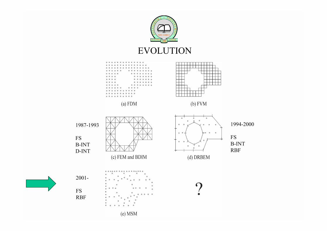
EVOLUTION
1994-2000
FSB-INTRBF
1987-1993
FSB-INTD-INT
2001-
FSRBF
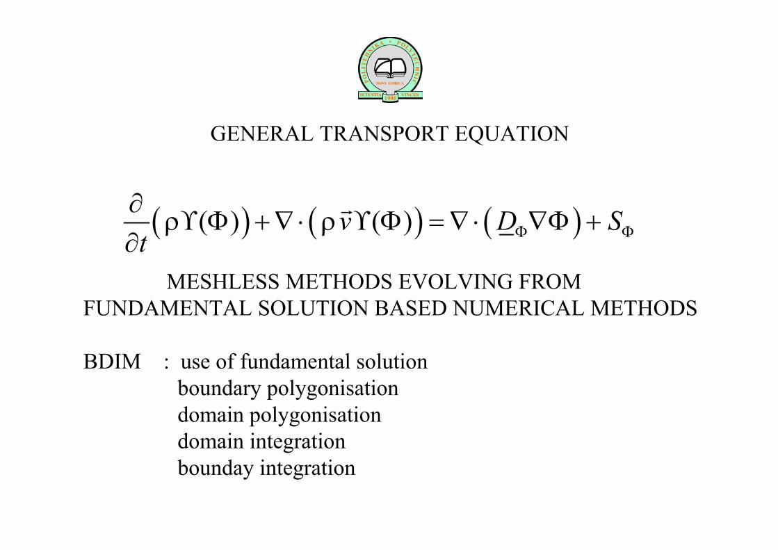
GENERAL TRANSPORT EQUATION
MESHLESS METHODS EVOLVING FROMFUNDAMENTAL SOLUTION BASED NUMERICAL METHODS
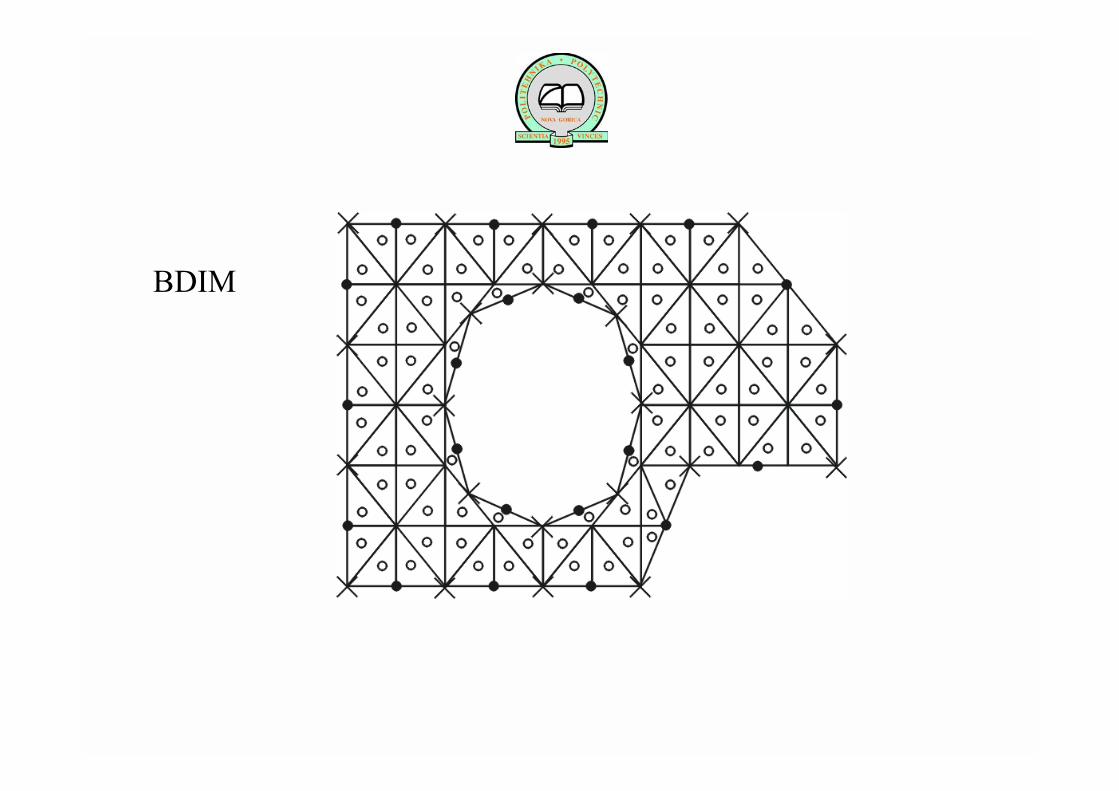
BDIM : use of fundamental solution boundary polygonisationdomain polygonisationdomain integrationbounday integration
( ) ( ) ( )( ) ( )v D Stρ ρ Φ Φ
∂ϒ Φ +∇ ⋅ ϒ Φ = ∇ ⋅ ∇Φ +
∂r
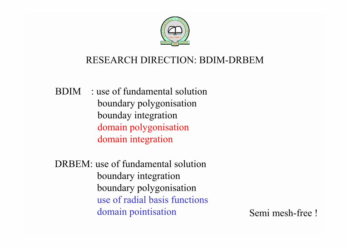
RESEARCH DIRECTION: BDIM-DRBEM
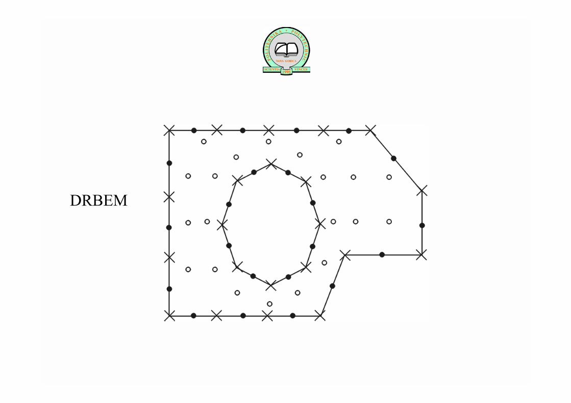
DRBEM: use of fundamental solutionboundary integration boundary polygonisationuse of radial basis functionsdomain pointisation
BDIM : use of fundamental solution boundary polygonisationbounday integration domain polygonisationdomain integration
Semi mesh-free !
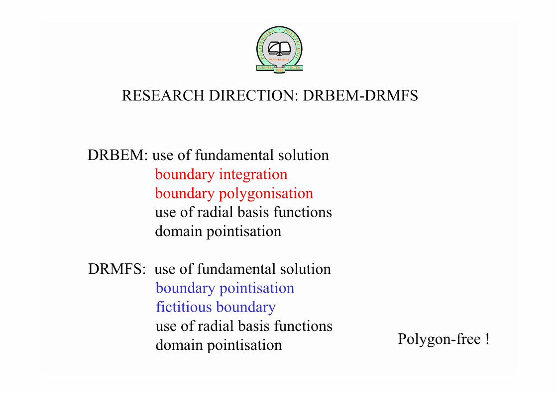
RESEARCH DIRECTION: DRBEM-DRMFS
DRBEM: use of fundamental solutionboundary integration boundary polygonisationuse of radial basis functions domain pointisation
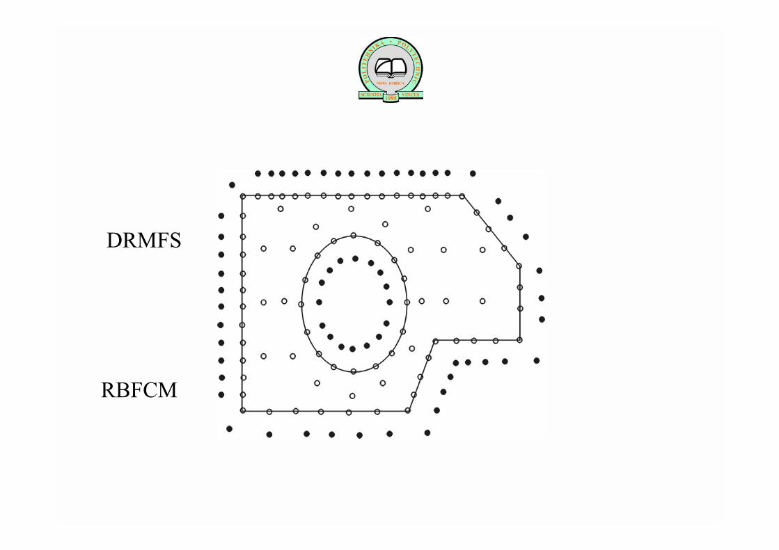
DRMFS: use of fundamental solution boundary pointisationfictitious boundaryuse of radial basis functionsdomain pointisation Polygon-free !

RESEARCH DIRECTION: DRMFS-RBFCM
DRMFS: use of fundamental solutionboundary pointisationfictitious boundaryuse of radial basis functions domain pointisation
RBFCM: boundary pointisationuse of radial basis functionsdomain pointisation
Polygon-free !
BDIM
DRBEM
DRMFS
RBFCM


Motivation
RBF interpolation
RBF solution of PDE
Advanced solution strategies
Natural convection in porous media - Darcy model
Thermal design of hollow bricks
Natural convection in solid-liquid system
Stefan problem
SCOPE

( ) ( )n np p sψ ψ= −r r
where is the Euclidean norm•
RADIAL BASIS FUNCTIONS
: is a continuous function R Rψ + →
(0) 0ψ ≥
is a continuous function ψ

; , ,p p i x y zξ ξ ξ= =rr
RADIAL BASIS FUNCTION APPROXIMATION
( ) ( )n np pψ ς≈r rF
1n nm mς −= Ψ F( ) ( )m m n m n mn np pψ ς ψ ς≡ = ≡r rF F
RBF Approximation
Calculation of Coefficients (Collocation, Least Squares)
Cartesian Coordinate System
( ) ( )n np p sψ ψ= −r r r

RADIAL BASIS FUNCTIONS - THEORY
1982 R. Franke: interpolation of scattered data, comparisonof different RBFs
1984 S. Stead: calculation of partial derivatives
1990 E.J. Kansa: approximation of surfaces1990 E.J. Kansa: parabolic, hyperbolic, elliptic PDE
1996 G.E. Fasshauer: symmetric solution of PDE1992 Z. Wu: Hermite-Birkhoff interpolation
nr3
nr2 2 where is a shape parameter.nr c c+
2
2 1
log , k 1, in 2D
, k 1, in 3D
kn n
kn
r r
r −
≥
≥22
nc re−
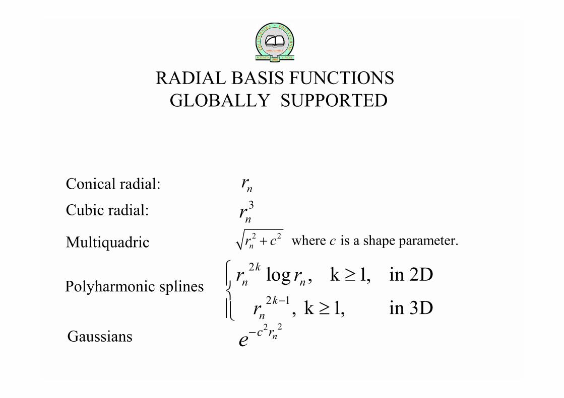
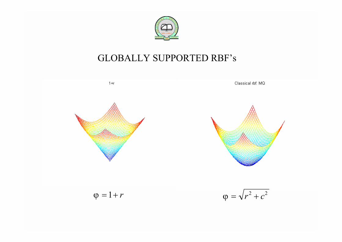
RADIAL BASIS FUNCTIONSGLOBALLY SUPPORTED
Conical radial:Cubic radial:
Multiquadric
Polyharmonic splines
Gaussians
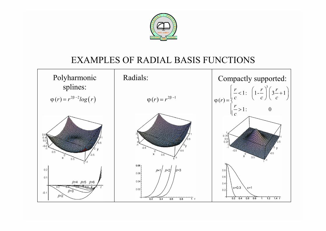
EXAMPLES OF RADIAL BASIS FUNCTIONS
Polyharmonic splines:
( )2 2( )r r log rβϕ −=
Radials:
2 1( )r r βϕ −=
Compactly supported:3
1: 1- 3 1( )
1: 0
r r rc c crrc
ϕ
< + = >
ϕ = +r c2 21 rϕ = +
GLOBALLY SUPPORTED RBFs

(1 ) , 0 1(1 )
0, 1
nn r r
rr+
− ≤ ≤− =
>For d=1: ϕ
ϕ
ϕ
= − ∈
= − + ∈
= − + + ∈
+
+
+
( )( ) ( )( ) (8 )
11 3 11 5 1
0
3 2
5 2 4
r Cr r Cr r r C
For d=2, 3: ϕ
ϕ
ϕ
ϕ
= − ∈
= − + ∈
= − + + ∈
= − + + + ∈
+
+
+
+
( )( ) ( )( ) ( )( ) ( )
11 4 11 35 18 31 32 25 8 1
2 0
4 2
6 2 4
8 3 2 6
r Cr r Cr r r Cr r r r C
Wendlands CS-RBFs
RADIAL BASIS FUNCTIONSCOMPACTLY SUPPORTED
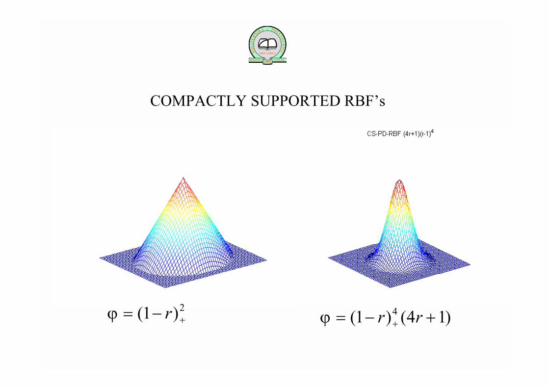
ϕ = − +( )1 2r ϕ = − ++( ) ( )1 4 14r r
COMPACTLY SUPPORTED RBFs

PARTICULAR SOLUTION ONCE AGAIN
θΦParticular solution satisfies the Poisson equation but not necessarily the boundary conditions
( ) ( )Φ−Φ⋅∇+⋅∇+Φ−Φ+=Φ∇ ΦΦ ,,2 ΘΘθθ
2n nψ ς∇ Φ =
2 n nψ ψ∇ =
n nψ ςΦ =
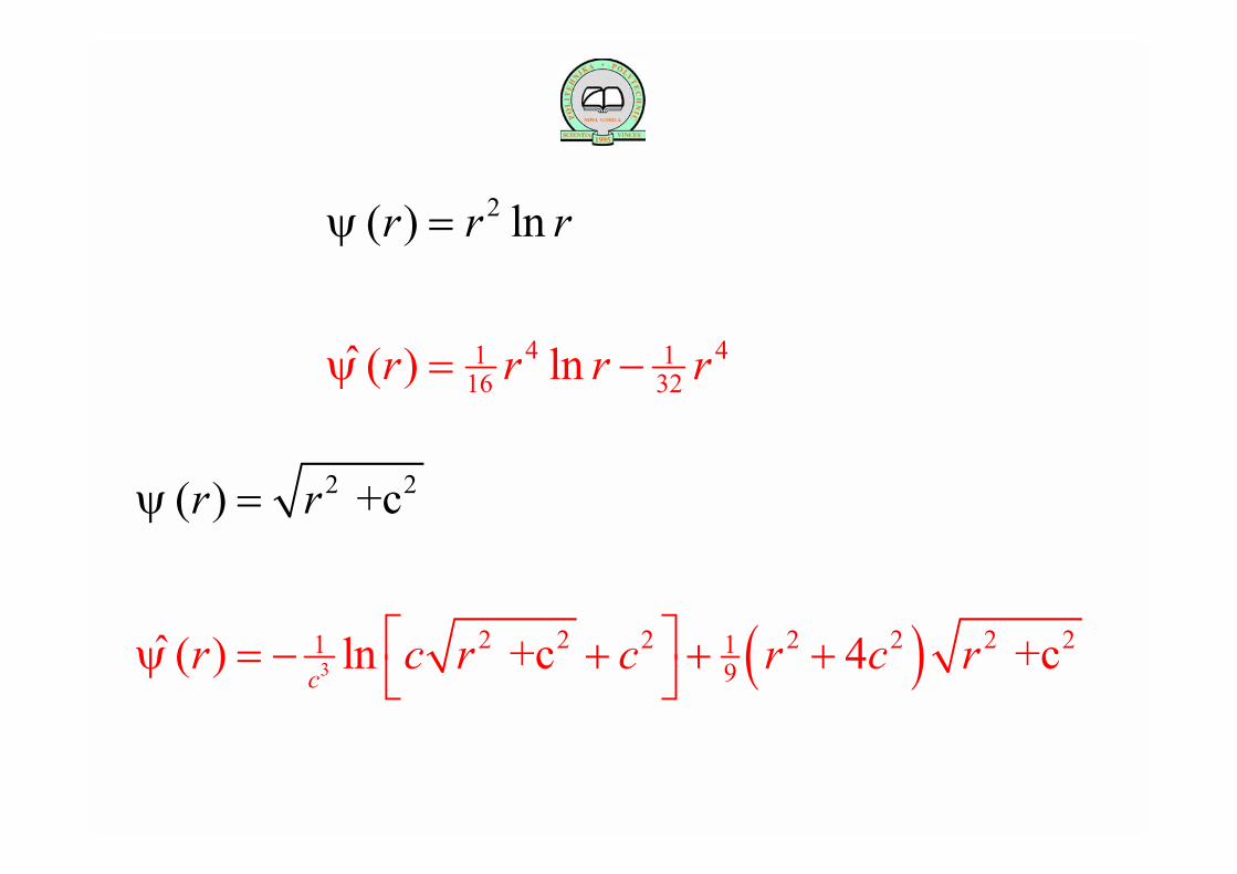
4
2
41 116 32 ( )
( ) l
ln
nr r
r
r
r r rψ
ψ =
= −
( )32 2 2 2 2 2 21 1
2 2
9 ( ) ln +c 4
( ) +c
c
+c
r c r r
r r
c c r
ψ
ψ = − + +
=
+

( ) ( )21 3
2 2 2 202 2
2rr c r cψ
− −= + + +
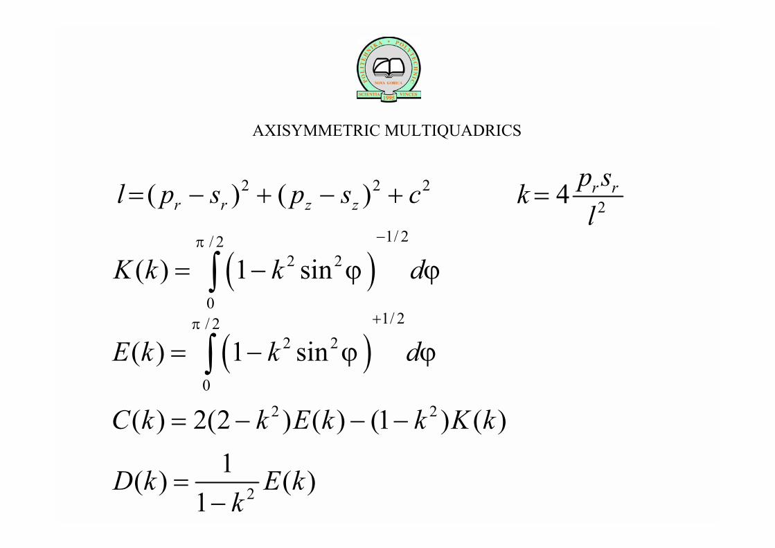
AXISYMMETRIC MULTIQUADRICS
( ) ( )21 1
2 2 2 202 2
4rr c r cψ
+ −= + − +
( )1
2 2 212
r cψ+
= +
( )3
2 2 2112
r cψ+
= +
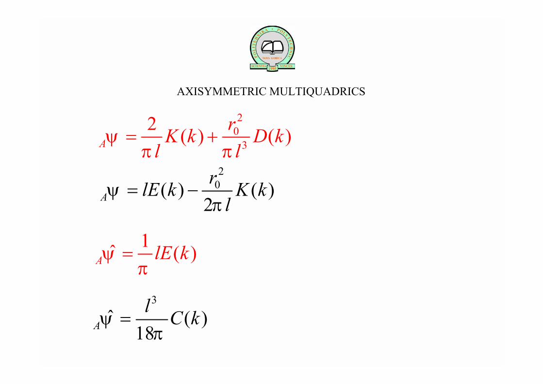
20
3
2 ( ) ( )ArK k D k
l lψ
π π= +
AXISYMMETRIC MULTIQUADRICS
1 ( )A lE kψπ
=
3
( )18Al C kψπ
=
20( ) ( )
2ArlE k K k
lψ
π= −
( )1/ 2/ 2
2 2
0
( ) 1 sinK k k dπ
ϕ ϕ−
= −∫
AXISYMMETRIC MULTIQUADRICS
( )1/ 2/ 2
2 2
0
( ) 1 sinE k k dπ
ϕ ϕ+
= −∫2 2( ) 2(2 ) ( ) (1 ) ( )C k k E k k K k= − − −
2
1( ) ( )1
D k E kk
=−
2 2 2( ) ( )r r z zl p s p s c= − + − + 24 r rp skl
=
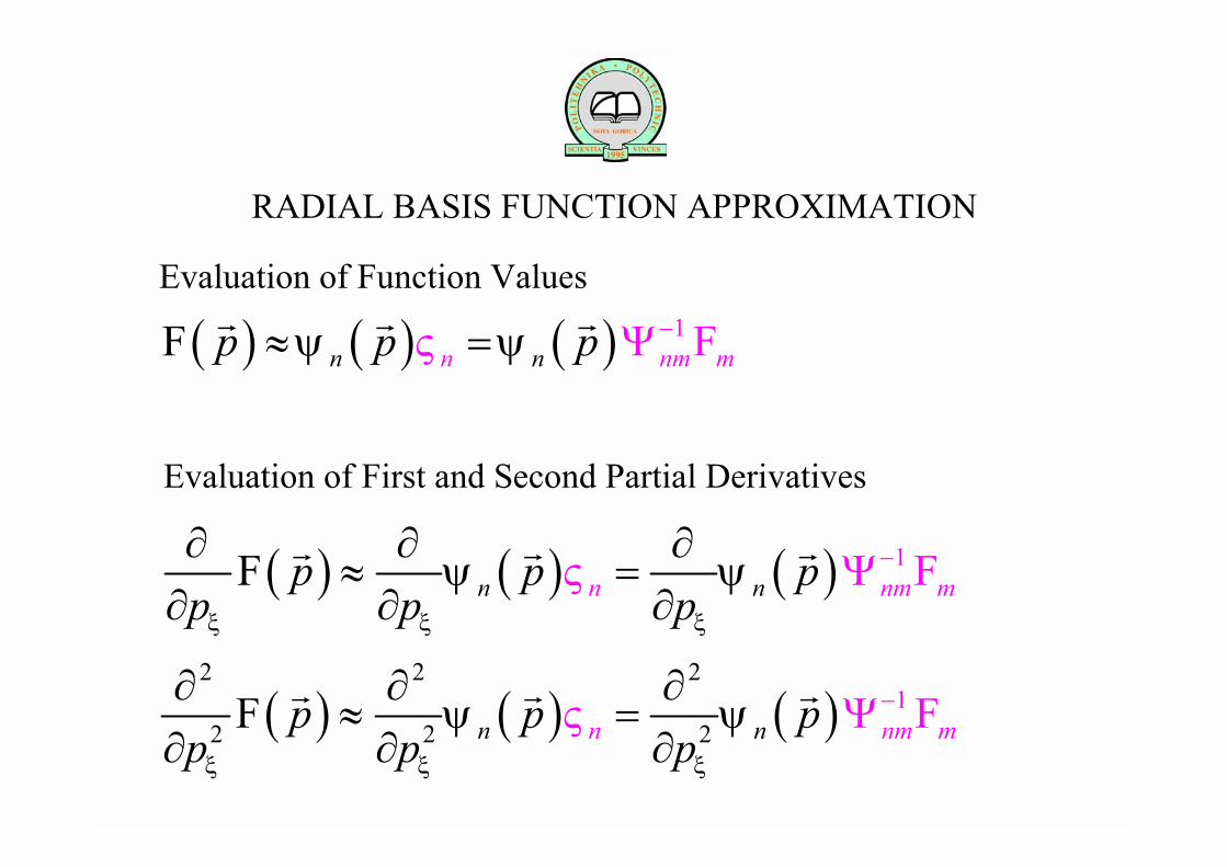
RADIAL BASIS FUNCTION APPROXIMATION
( ) ( ) ( ) 1n n nmn mp p pψ ψς −≈ = Ψ
r r rF F
( ) ( ) ( ) 1nn n nm mp p p
p p pξ ξ ξ
ςψ ψ −∂ ∂ ∂≈ =
∂ ∂Ψ
∂r r r FF
( ) ( ) ( )2 2 2
2 2 21
n nn nm mp p pp p pξ ξ ξ
ςψ ψ −∂ ∂ ∂≈ =
∂ ∂Ψ
∂r r r FF
Evaluation of Function Values
Evaluation of First and Second Partial Derivatives
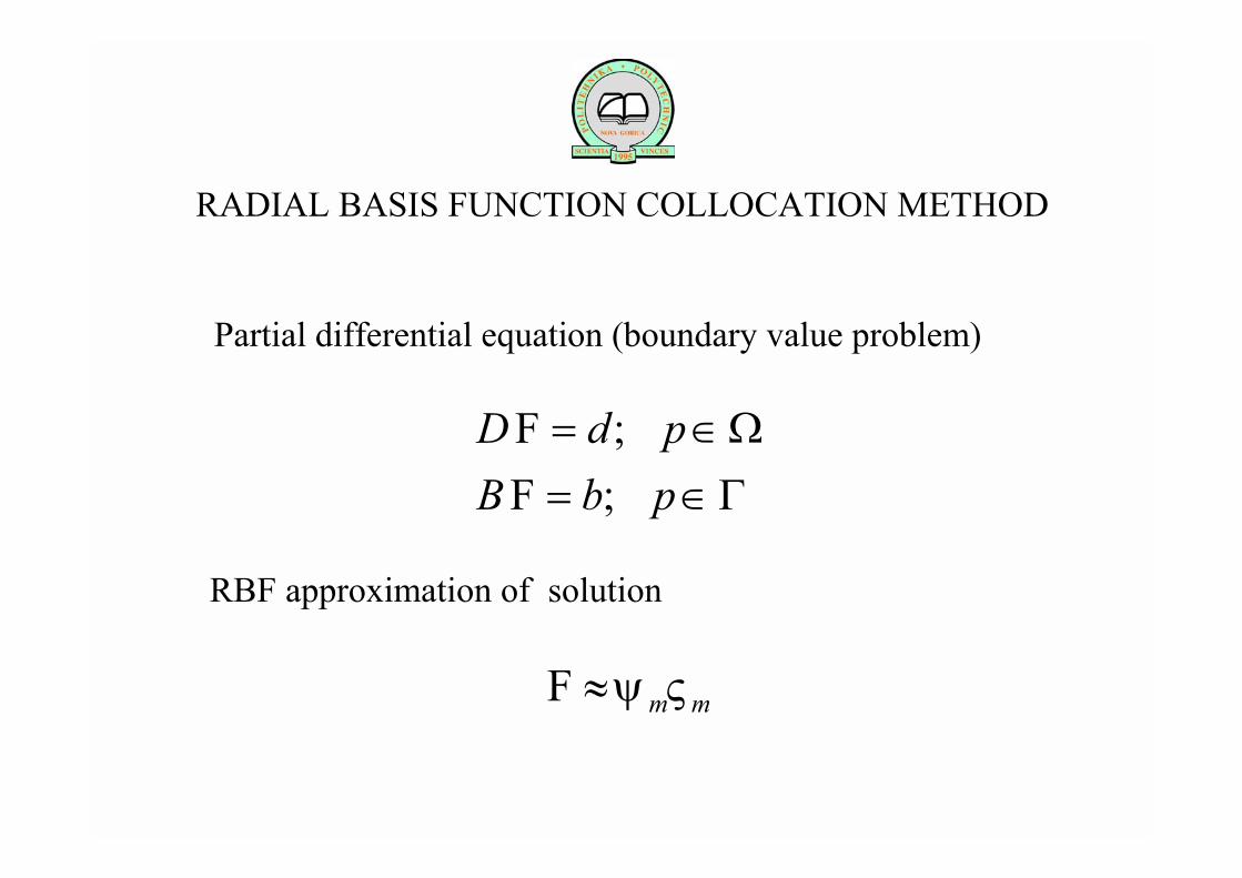
RADIAL BASIS FUNCTION COLLOCATION METHOD
;;
D d pB b p
= ∈Ω= ∈Γ
FF
m mψ ς≈F
Partial differential equation (boundary value problem)
RBF approximation of solution
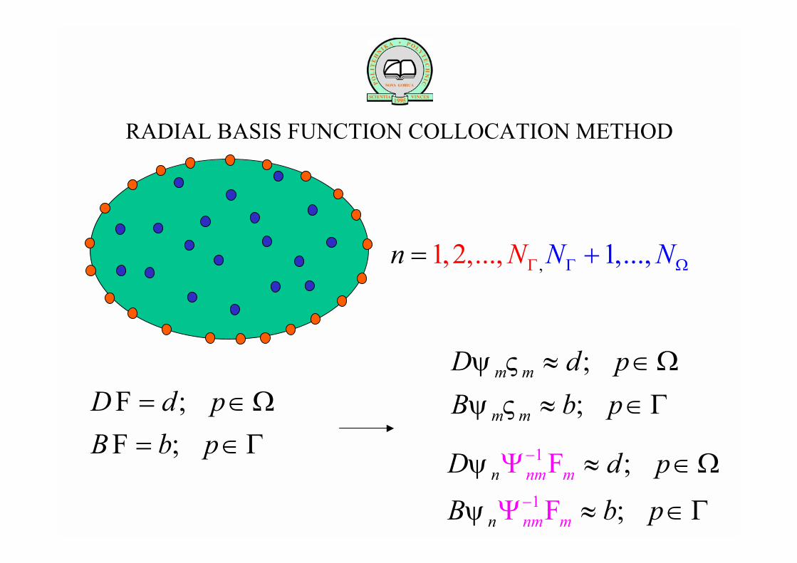
RADIAL BASIS FUNCTION COLLOCATION METHOD
;;
D d pB b p
= ∈Ω= ∈Γ
FF
;;
m m
m m
D d pB b pψ ςψ ς
≈ ∈Ω≈ ∈Γ
1
1
;
;nm m
nm
n
mn
D d p
B b p
ψ
ψ
−
−
≈ ∈Ω
≈ ∈
Ψ
Ψ Γ
F
F
,1,2,... 1, ,...,n NN NΓ ΩΓ +=
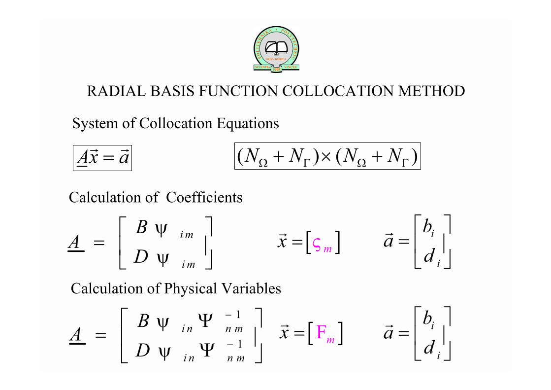
RADIAL BASIS FUNCTION COLLOCATION METHOD
Ax a=r r
i
i
ba
d
=
ri m
i m
BA
Dψψ
=
1
1i n n m
i n n m
BA
Dψψ
−
−
Ψ= Ψ
[ ]mx ς=r
[ ]mx =r F i
i
ba
d
=
r
Calculation of Coefficients
Calculation of Physical Variables
System of Collocation Equations
( ) ( )N N N NΩ Γ Ω Γ+ × +

RADIAL BASIS FUNCTION COLLOCATION METHOD
1 1
( ) ( )N N
s n n s n nn n N
B Dψ ς ψ ςΓ Ω
Γ= = +
≈ +∑ ∑F
Symmetric approximation
,s sB D adjoint operators acting on sr
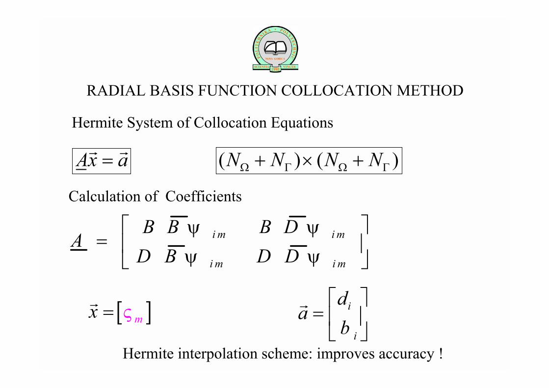
RADIAL BASIS FUNCTION COLLOCATION METHOD
Ax a=r r
i
i
da
b
=
r
i m i m
i m i m
B B B DA
D B D Dψ ψψ ψ
=
[ ]mx ς=r
Calculation of Coefficients
Hermite System of Collocation Equations
Hermite interpolation scheme: improves accuracy !
( ) ( )N N N NΩ Γ Ω Γ+ × +
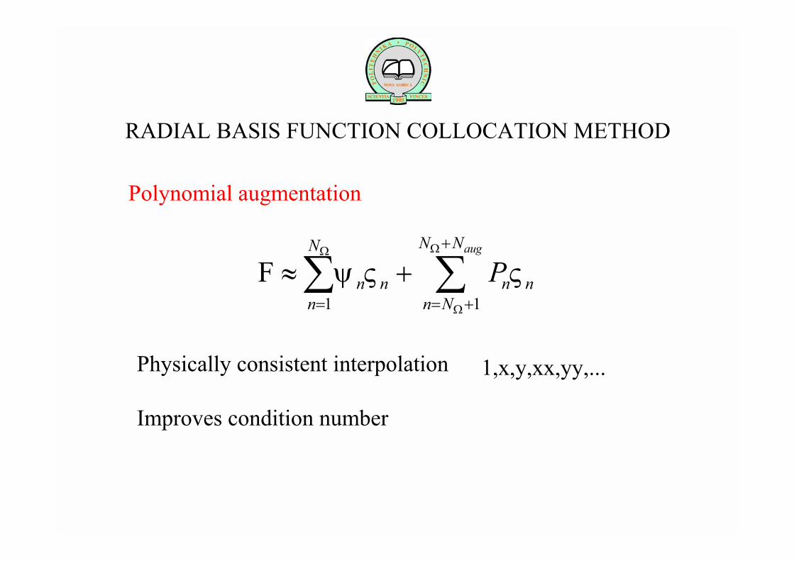
RADIAL BASIS FUNCTION COLLOCATION METHOD
1 1
augN NN
n n n nn n N
Pψ ς ςΩΩ
Ω
+
= = +
≈ +∑ ∑F
Polynomial augmentation
Physically consistent interpolation
Improves condition number
1,x,y,xx,yy,...
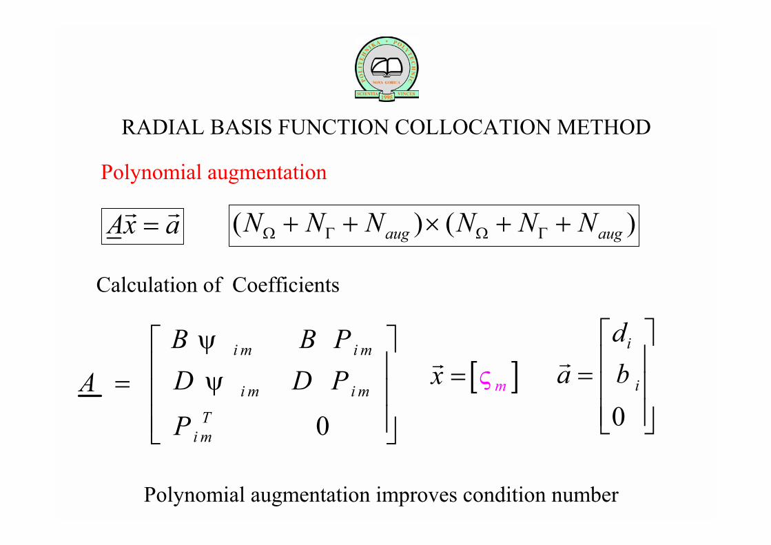
RADIAL BASIS FUNCTION COLLOCATION METHOD
Ax a=r r
0
i
i
dba =
r
0
i m i m
i m i m
Ti m
B B PD D PAP
ψψ
=
Calculation of Coefficients
Polynomial augmentation
Polynomial augmentation improves condition number
( ) ( )aug augN N N N N NΩ Γ Ω Γ+ + × + +
[ ]mx ς=r
RADIAL BASIS FUNCTION COLLOCATION METHOD
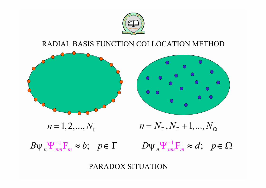
1 ;mn nmB b pψ − ≈ ΓΨ ∈F 1 ;mn nmD d pψ − ≈ ΩΨ ∈F
PARADOX SITUATION
1,2,...,n NΓ= , 1,...,n N N NΓ Γ Ω= +

RADIAL BASIS FUNCTION COLLOCATION METHOD
D d=F=
RBF approximation
* *D d ddΩ Ω
Ω = Ω∫ ∫F=F F
** * *s sc dd d d
n nΓ ΓΩ Γ Γ
∂ ∂= Ω+ Γ − Γ
∂ ∂∫ ∫ ∫F FF F F= F
Green formula
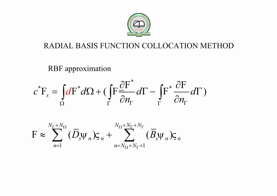
RADIAL BASIS FUNCTION COLLOCATION METHOD
RBF approximation*
* * *( )sc d d dn n
dΓ ΓΩ Γ Γ
∂ ∂= Ω+ Γ − Γ
∂ ∂∫ ∫ ∫F FF F F= F
1 1
( ) ( )N N N N N
s n n s n nn n N N
D Bψ ς ψ ςΓ Ω Ω Γ Γ
Ω Γ
+ + +
= = + +
≈ +∑ ∑F
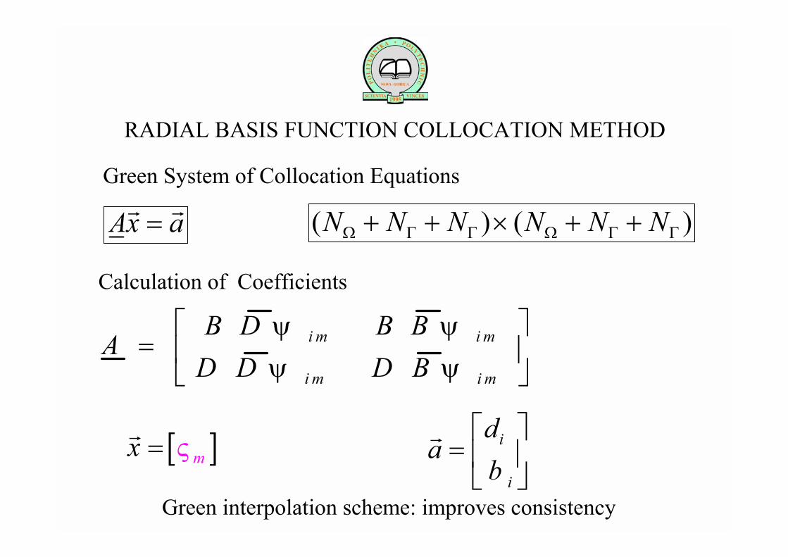
RADIAL BASIS FUNCTION COLLOCATION METHOD
Ax a=r r
i
i
da
b
=
r
i m i m
i m i m
B D B BA
D D D Bψ ψψ ψ
=
[ ]mx ς=r
Calculation of Coefficients
Green System of Collocation Equations
Green interpolation scheme: improves consistency
( ) ( )N N N N N NΩ Γ Γ Ω Γ Γ+ + × + +

RADIAL BASIS FUNCTIONS - TRANSPORT PHENOMENA
1998 M. Zerroukat, H. Power, C.S. Chen: heat conduction
2000 M. Zerroukat, K. Djidjeli, A. Charafi: advection-diffusion
2001 B. arler, J. Perko, C.S. Chen: Navier-Stokes
2001 J. Perko, B. arler: Solid-liquid phase change (FBP)
2002 H. Power, V. Barraco: unsymmetric versus symmetric
2002 W. Chen, Green interpolation scheme - proposal2003 B. arler, R. Vertnik, Green interpolation scheme - application
1996 G. E. Fasshauer, Hermite interpolation scheme
2003 I. Kovačević, B. arler, Stefan problem (MBP)
DΓ
NΓ
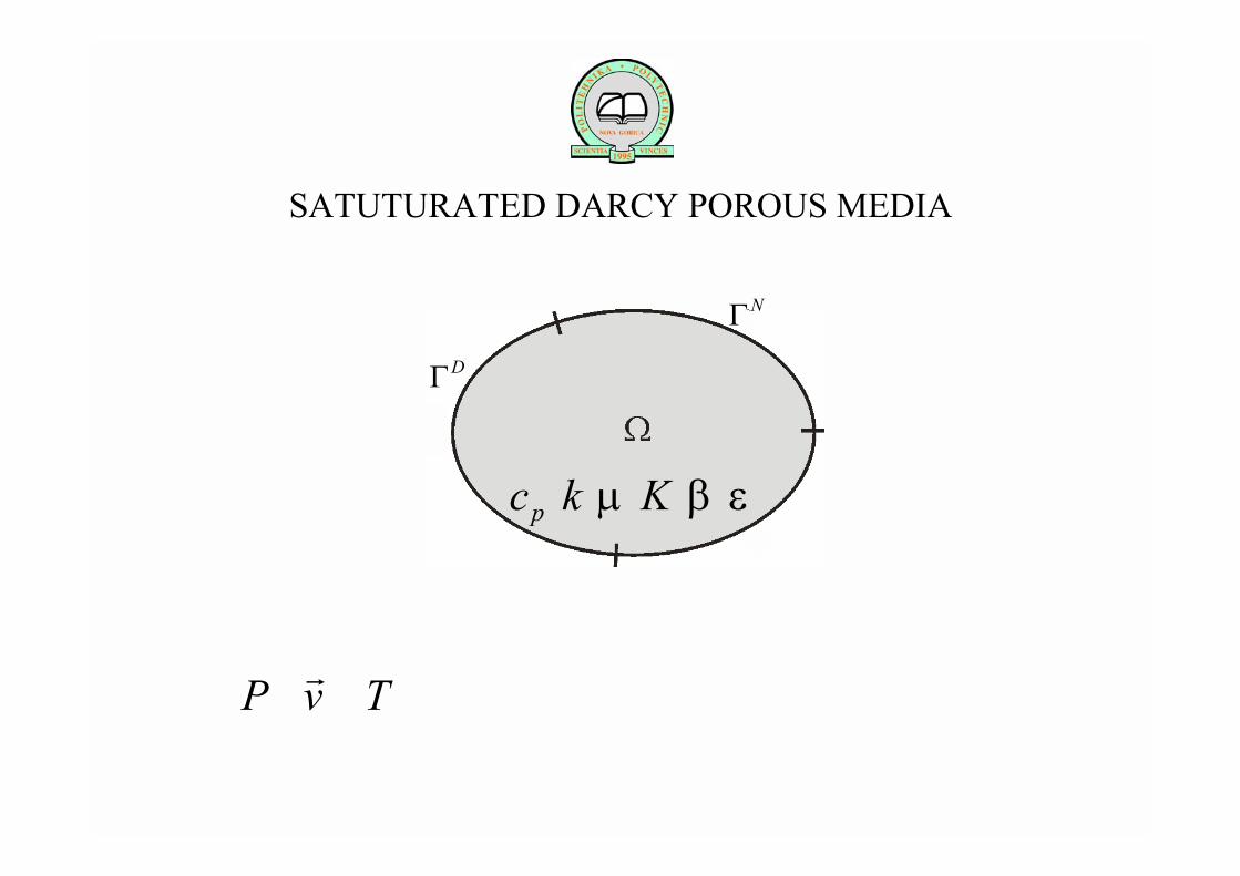
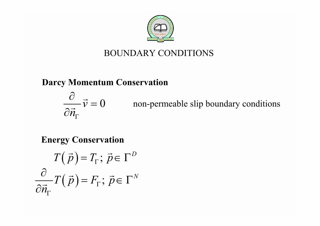
SATUTURATED DARCY POROUS MEDIA
P v Tr
pc k Kµ β ε

0 p v fKµ
= −∇ − +rrDarcy Momentum Conservation
0v∇ ⋅ =rMass Conservation
1 ( )reff a T Tρ β = − − r r
Boussinesq Body Force
Energy Conservation 2( )pc vT k Tρ ∇ ⋅ = ∇r
GOVERNING EQUATIONS

PREVIOUS APPROACHES
1970 FDM: B.K.C. Chan, C.M. Ivey, J.M. Barry
1981 FEM: G.E. Hickox, C.M. Gartling
1984 FVM: V. Prasad, F.A. Kulacki
2001 BDIM: R. Jecl, L. kerget, E. Petriin
2000 DRBEM: B. arler, D. Gobin, B. Goyeau, J. Perko, H. Power

DΓ
NΓ
RBFCM SOLUTION STRATEGY
P v Tr
•
•
••
•
••
•••
•
•••
•
•
••
•
•
•
•
•
( ) ( )n np p sψ ψ= −r r r
nprpc k Kµ β εinterpolation
solution
( ) ( )n np pψ ςΦ ≈r r
0vnΓ
∂=
∂r
r
Darcy Momentum Conservation
Energy Conservation
( ) ; DT p T pΓ= ∈Γr r
BOUNDARY CONDITIONS
( ) ; NT p F pn ΓΓ
∂= ∈Γ
∂r r
r
non-permeable slip boundary conditions
12 ( );jj jv f pK
P µ+∇ = ∇ ⋅ − + ∈Ωrr r
1 ( ) ; j jjP n v f n pKµ
Γ Γ+∇ ⋅ = − + ⋅ ∈Γ
rr r r r
1 ; jj f n pn
P ΓΓ
+∂= ⋅ ∈Γ
∂
r r rr
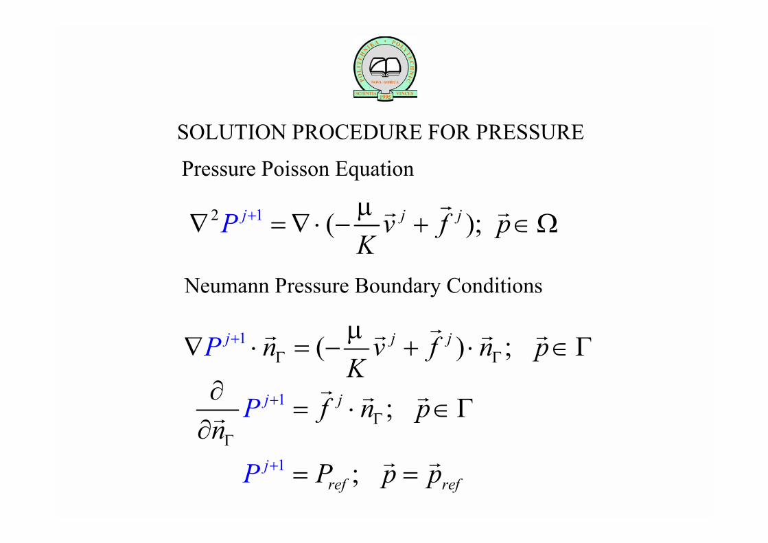
SOLUTION PROCEDURE FOR PRESSURE
Pressure Poisson Equation
Neumann Pressure Boundary Conditions
1 ; ref ej
r fP P p p+ = =r r

1 1 ( ); ,j j jv P f x yKξ ξµ
ξξ
+ +∂= − + =
∂
r
11 1( ) 0jj jv v v+ ++∇ ⋅ = ∇ ⋅ + =r%r r
SOLUTION PROCEDURE FOR VELOCITY
1 11 jj jv v v +++ = +r%r r
Does not obey mass conservation in general !

1 1 1 1( )j j j jP v v vK Kµ µ+ + + +∇ = − = − −r r r%%
2 1 1j jP vKµ+ +∇ =+ ∇ ⋅
r%
1 0; jP pn
+
Γ
∂= ∈Γ
∂r%r
SOLUTION PROCEDURE FOR PRESSURE CORRECTION
Neumann Pressure Correction Boundary Conditions
Pressure Correction Poisson Equation
1 0; jrefP p p+ = =
r r%

SOLUTION PROCEDURE FOR CORRECTED VELOCITY
BODY FORCE UPDATING
1 1 1 j P jre
jl
Kc Pv vpξξξµ
+ + +∂= −
∂%
( )( )1 1j j f jrel
jTf f c f f++ = + −
SOLUTION PROCEDURE FOR TEMPERATURE
1jT +
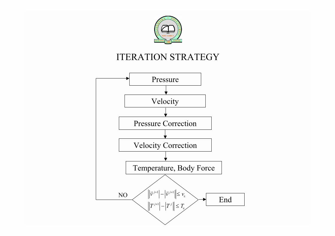
Pressure
Velocity
Pressure Correction
Temperature, Body Force
1 1
1
j j
j j
v v v
T T T
ε
ε
+ +
+
− ≤
− ≤
r r
EndNO
ITERATION STRATEGY
Velocity Correction

PRESSURE POISSON EQUATIONALGEBRAIC SYSTEM OF COLLOCATION EQUATIONS
1 1 ji n i nm
jm i in f n
pPξ ξ ξ
ξ
ψ Γ+−
Γ∂
Ψ =∂
Boundary Nodes
Domain Nodes
2 21 1
2 21 j
in in nm in nmx
jm
y
fp p p
P ξξ
ψ ψ ψ− −+ ∂ ∂ ∂
+ Ψ = Ψ ∂ ∂ ∂ 1
ref
jN m m refP Pδ + =

PRESSURE CORRECTION POISSON EQUATIONALGEBRAIC SYSTEM OF COLLOCATION EQUATIONS
1 1 0i n i nj
mmnp
Pξξ
ψ −Γ
+∂Ψ =
∂%
Boundary Nodes
Domain Nodes
2 21 1 1
21
2 j
in in nm n nx y
m mj
i vPp p K p ξ
ξ
µψ ψ ψ− + − +
∂ ∂ ∂+ Ψ = Ψ ∂ ∂ ∂
%
1 0ref m
jN mPδ + =%
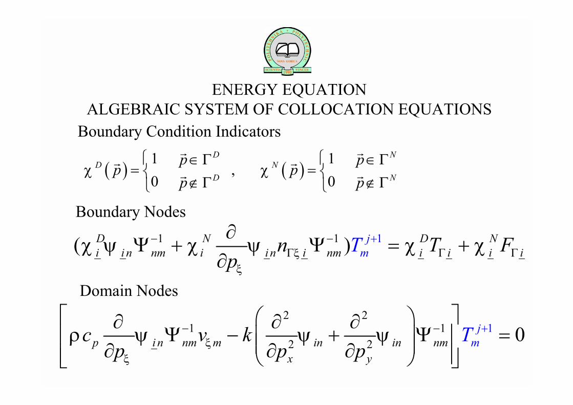
ENERGY EQUATIONALGEBRAIC SYSTEM OF COLLOCATION EQUATIONS
( ) ( )1 1
,0 0
D ND N
D N
p pp p
p pχ χ
∈Γ ∈Γ= =
∉Γ ∉Γ
r rr r
r r
Boundary Nodes
Domain Nodes
1 1 1( )D N D Ni i n nm i i n i
jnm i i i imn T F
pTξ
ξ
χ ψ χ ψ χ χ− −Γ Γ Γ
+∂Ψ + Ψ = +
∂
2 21 1 1
2 2 0p i n nm m in in nmx y
jmc v k
p p pTξ
ξ
ρ ψ ψ ψ− − + ∂ ∂ ∂
Ψ − + Ψ = ∂ ∂ ∂
Boundary Condition Indicators
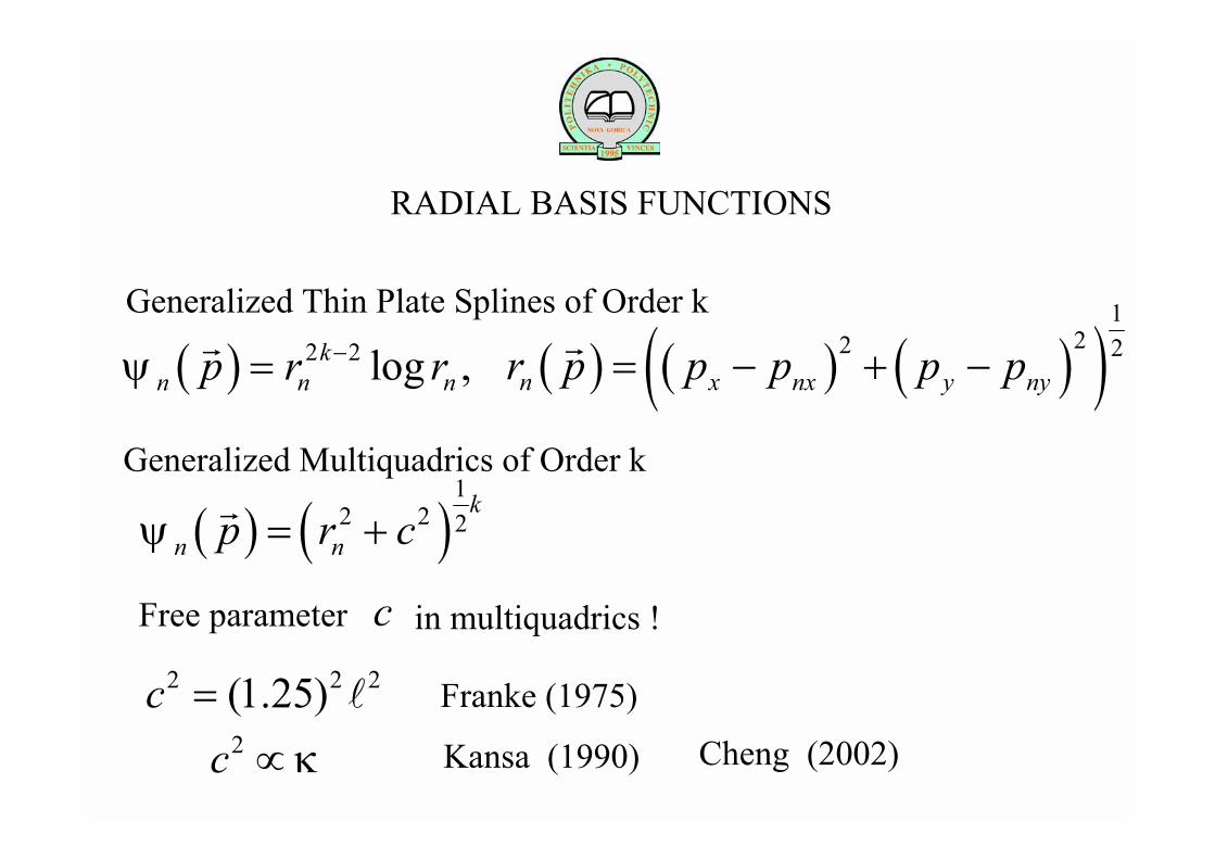
Generalized Thin Plate Splines of Order k
( ) 2 2 log ,kn n np r rψ −=
r
Generalized Multiquadrics of Order k
( ) ( )1
2 2 2k
n np r cψ = +r
( ) ( ) ( )( )1
22 2n x nx y nyr p p p p p= − + −
r
Free parameter c in multiquadrics !
RADIAL BASIS FUNCTIONS
2 2 2(1.25)c = l Franke (1975)
Kansa (1990)2c κ∝ Cheng (2002)
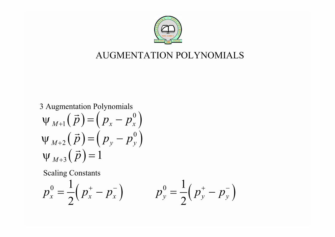
( ) ( )01M x xp p pψ + = −
r
( ) ( )02M y yp p pψ + = −
r
( )3 1M pψ + =r
3 Augmentation Polynomials
Scaling Constants
( )0 12x x xp p p+ −= − ( )0 1
2y y yp p p+ −= −
AUGMENTATION POLYNOMIALS
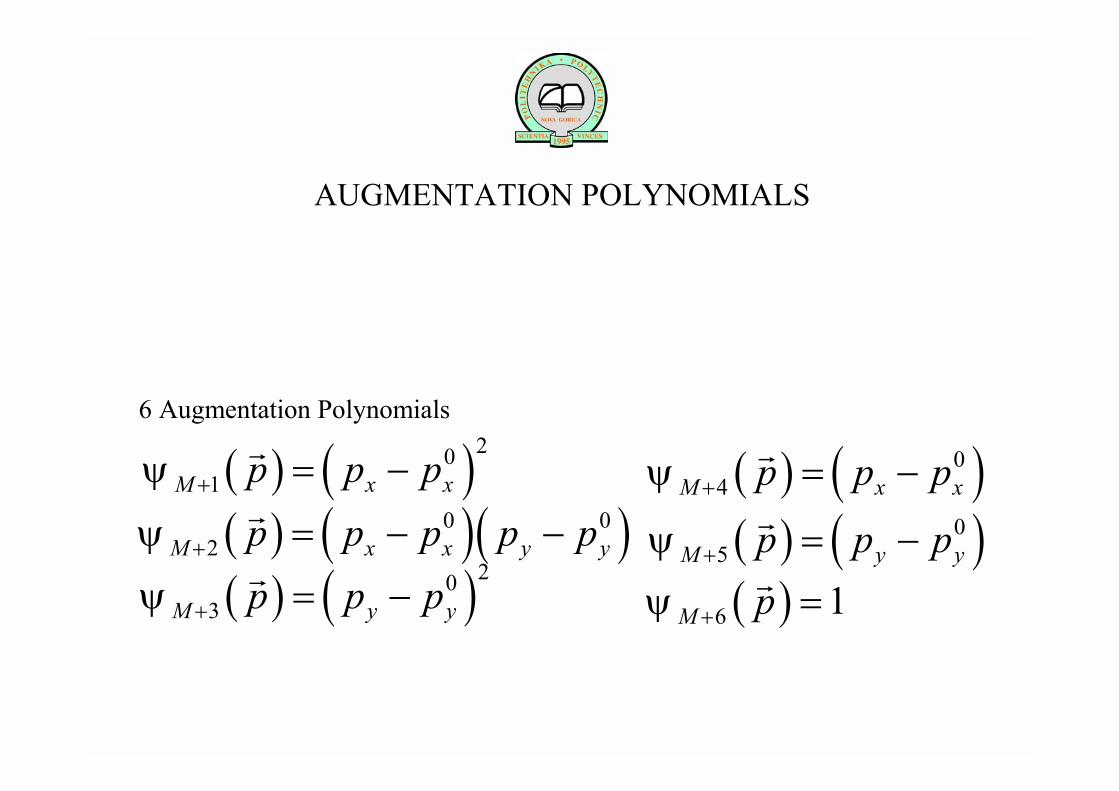
( ) ( )201M x xp p pψ + = −
r
( ) ( )( )0 02M x x y yp p p p pψ + = − −
r
( ) ( )203M y yp p pψ + = −
r
( ) ( )04M x xp p pψ + = −
r
( ) ( )05M y yp p pψ + = −
r
( )6 1M pψ + =r
6 Augmentation Polynomials
AUGMENTATION POLYNOMIALS

( , ) 0x yv p pnΓ
∂=
∂r
r
W E
N
S
( , )x yT p p T− +=
( , ) 0x yT p pn
+
Γ
∂=
∂r
NUMERICAL EXAMPLE
( , )x yT p p T+ −=
( , ) 0x yT p pn
−
Γ
∂=
∂r

NUMERICAL EXAMPLE-DIMENSIONLESS FORM0p p
pp
ξ ξξ
ξ
−=
∆
y
x
pA
p∆
=∆
p p pξ ξ ξ+ −∆ = −
2* p yc Ka p T
Rak
ρ β
µ
∆ ∆=
refT TT
T−
=∆
p yc pv v
kρ ∆
= p yc K pP v
kρ
µ
∆=
T T T+ −∆ = −
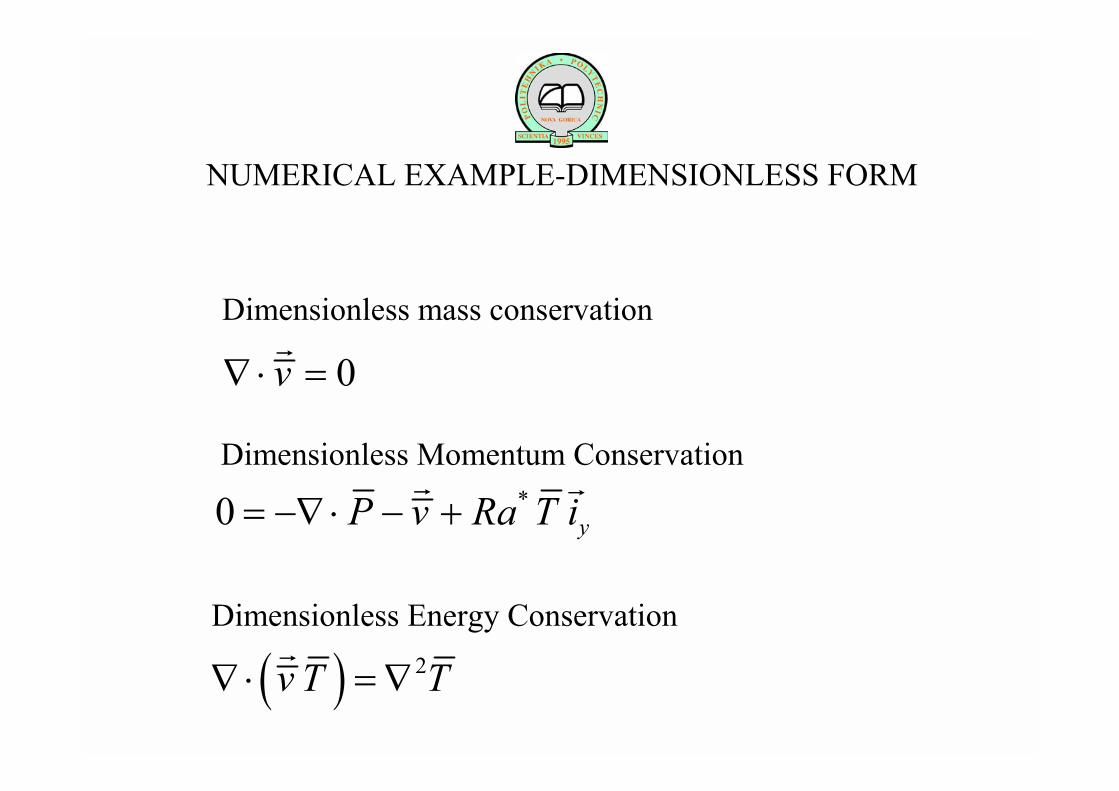
NUMERICAL EXAMPLE-DIMENSIONLESS FORM
0v∇ ⋅ =r
*0 yP v Ra T i= −∇ ⋅ − +r r
( ) 2v T T∇ ⋅ = ∇r
Dimensionless mass conservation
Dimensionless Momentum Conservation
Dimensionless Energy Conservation
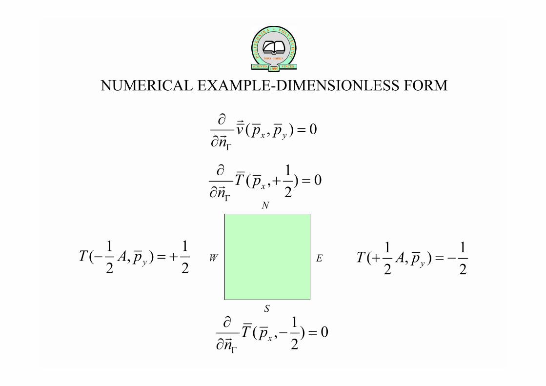
( , ) 0x yv p pnΓ
∂=
∂
rr
W E
N
S
1 1( , )2 2yT A p− = +
1( , ) 02xT p
nΓ
∂+ =
∂r
NUMERICAL EXAMPLE-DIMENSIONLESS FORM
1 1( , )2 2yT A p+ = −
1( , ) 02xT p
nΓ
∂− =
∂r
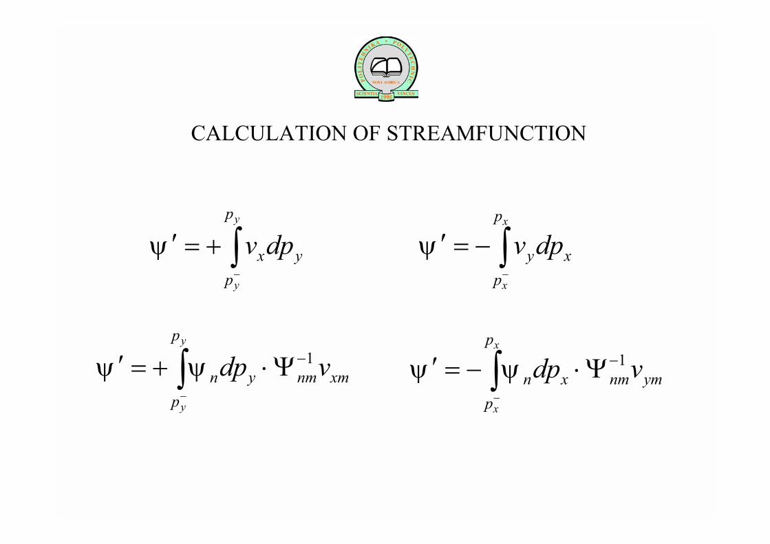
CALCULATION OF STREAMFUNCTION
y
y
p
x yp
v dpψ−
′ = + ∫x
x
p
y xp
v dpψ−
′ = − ∫
1y
y
p
n y nm xmp
dp vψ ψ−
−′ = + ⋅Ψ∫ 1x
x
p
n x nm ymp
dp vψ ψ−
−′ = − ⋅Ψ∫
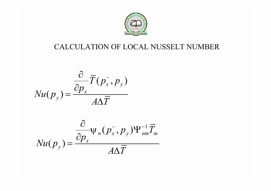
CALCULATION OF LOCAL NUSSELT NUMBER
( , )( )
x yx
y
T p ppNu p
A T
−∂∂
=∆
1( , )( )
n x y nm mx
y
p p TpNu p
A T
ψ − −∂Ψ
∂=
∆
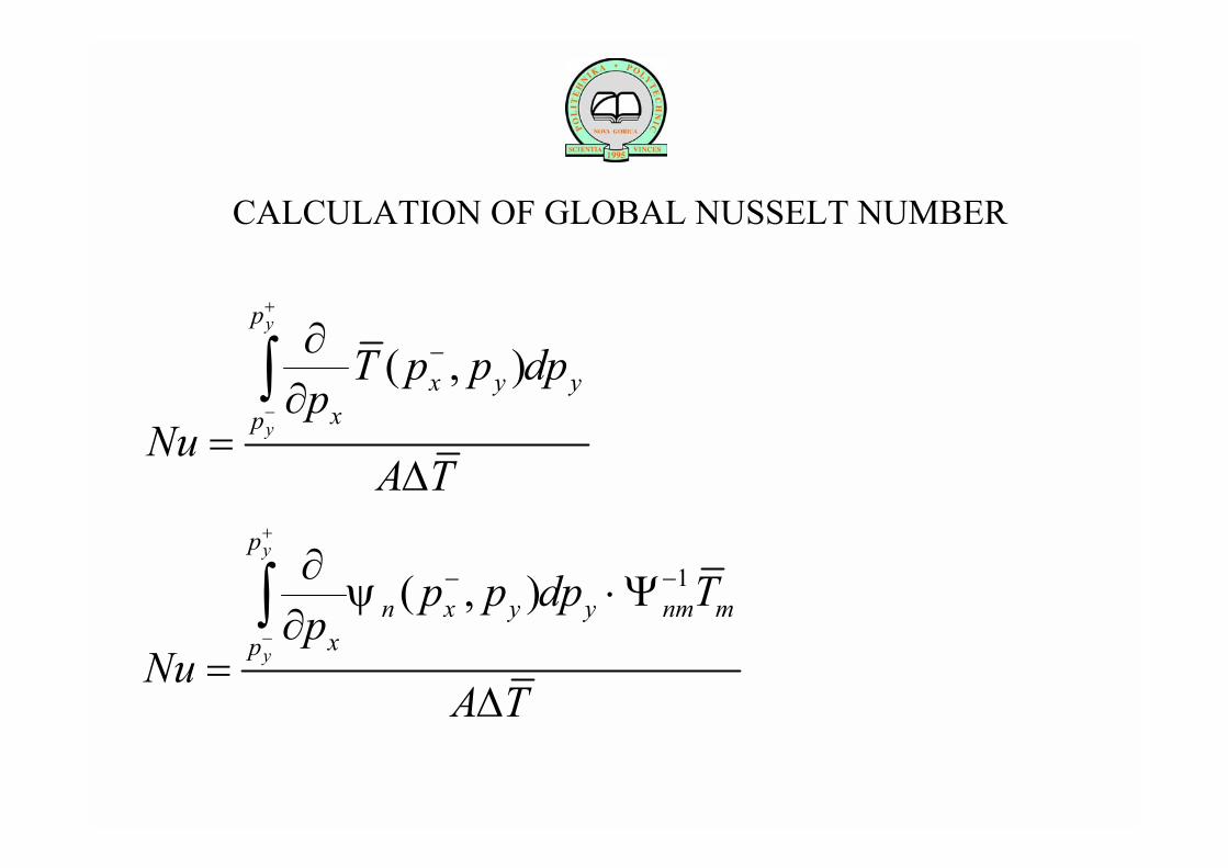
CALCULATION OF GLOBAL NUSSELT NUMBER
( , )y
y
p
x y yxp
T p p dpp
NuA T
+
−
−∂∂
=∆
∫
1( , )y
y
p
n x y y nm mxp
p p dp Tp
NuA T
ψ
+
−
− −∂ ⋅Ψ∂
=∆
∫

CALCULATION PARAMETERS
0.5Prelc =
0.001frelc =
0.0001vε =
0.0001Tε =
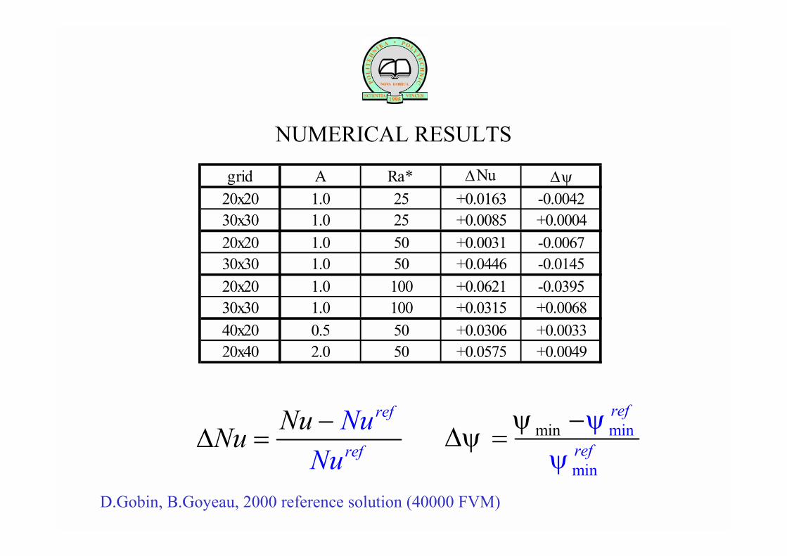
grid A Ra* ∆Nu ∆ψ20x20 1.0 25 +0.0163 -0.004230x30 1.0 25 +0.0085 +0.000420x20 1.0 50 +0.0031 -0.006730x30 1.0 50 +0.0446 -0.014520x20 1.0 100 +0.0621 -0.039530x30 1.0 100 +0.0315 +0.006840x20 0.5 50 +0.0306 +0.003320x40 2.0 50 +0.0575 +0.0049
ref
ref
NuN
NuNuu−
∆ = min
m
min
in
ref
ref
ψψ
ψψ
−∆ =
NUMERICAL RESULTS
D.Gobin, B.Goyeau, 2000 reference solution (40000 FVM)
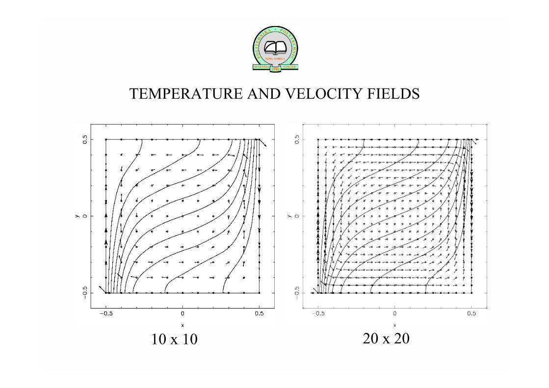
TEMPERATURE AND VELOCITY FIELDS
10 x 10 20 x 20
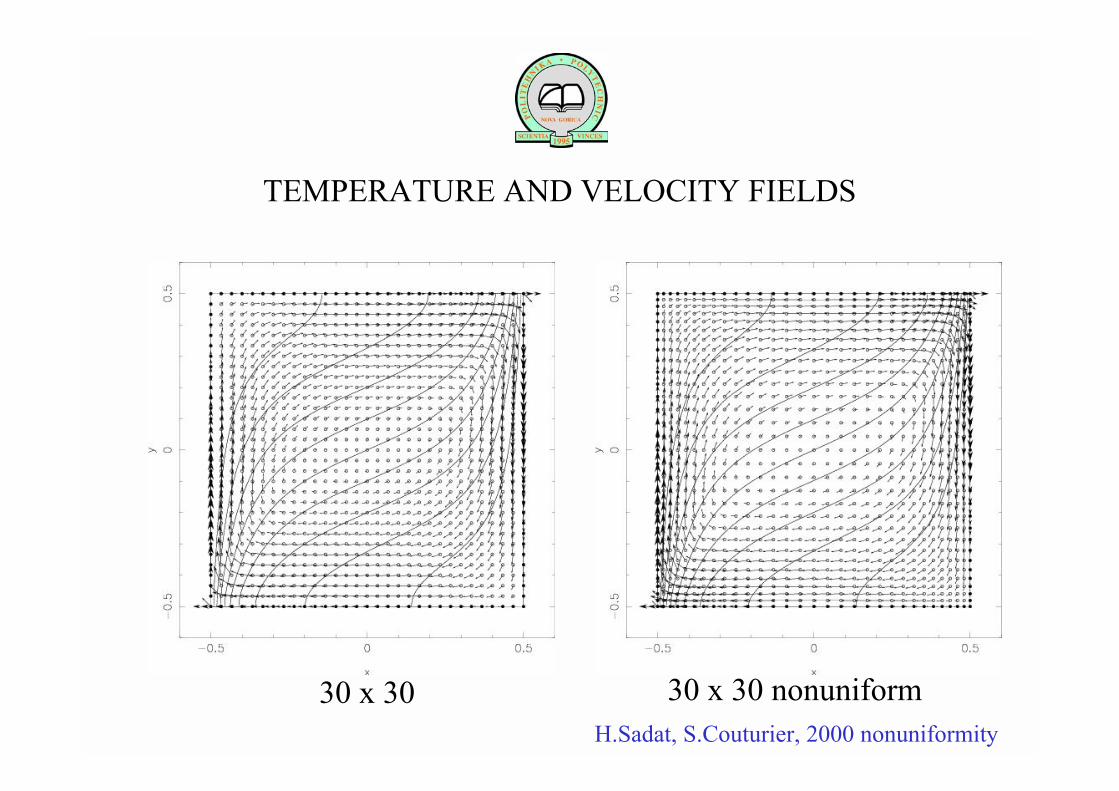
TEMPERATURE AND VELOCITY FIELDS
30 x 30 30 x 30 nonuniformH.Sadat, S.Couturier, 2000 nonuniformity
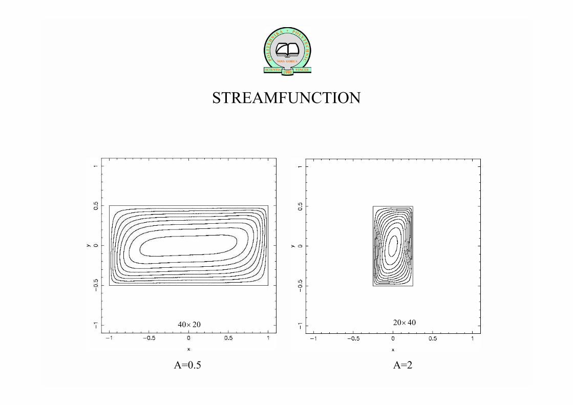
STREAMFUNCTION
A=0.5 A=2
40 20× 20 40×

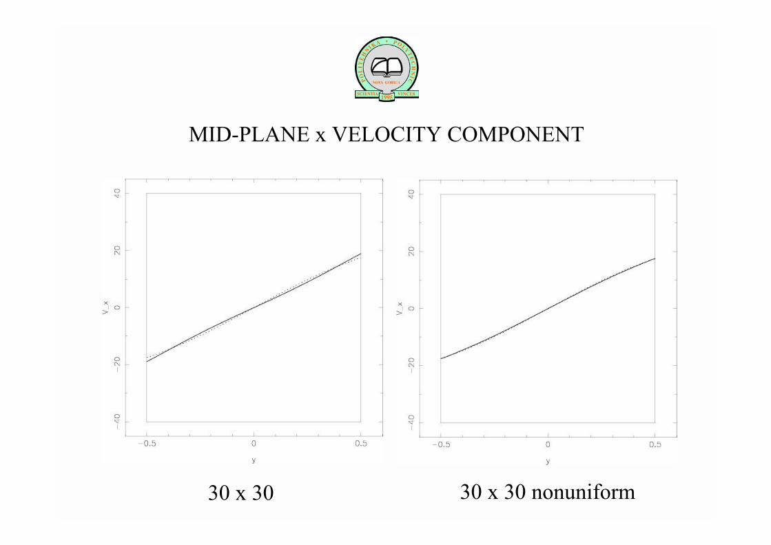
MID-PLANE x VELOCITY COMPONENT
10 x 10 20 x 20
MID-PLANE x VELOCITY COMPONENT
30 x 30 30 x 30 nonuniform

MID-PLANE y VELOCITY COMPONENT
10 x 10 20 x 20

MID-PLANE y VELOCITY COMPONENT
30 x 30 30 x 30 nonuniform
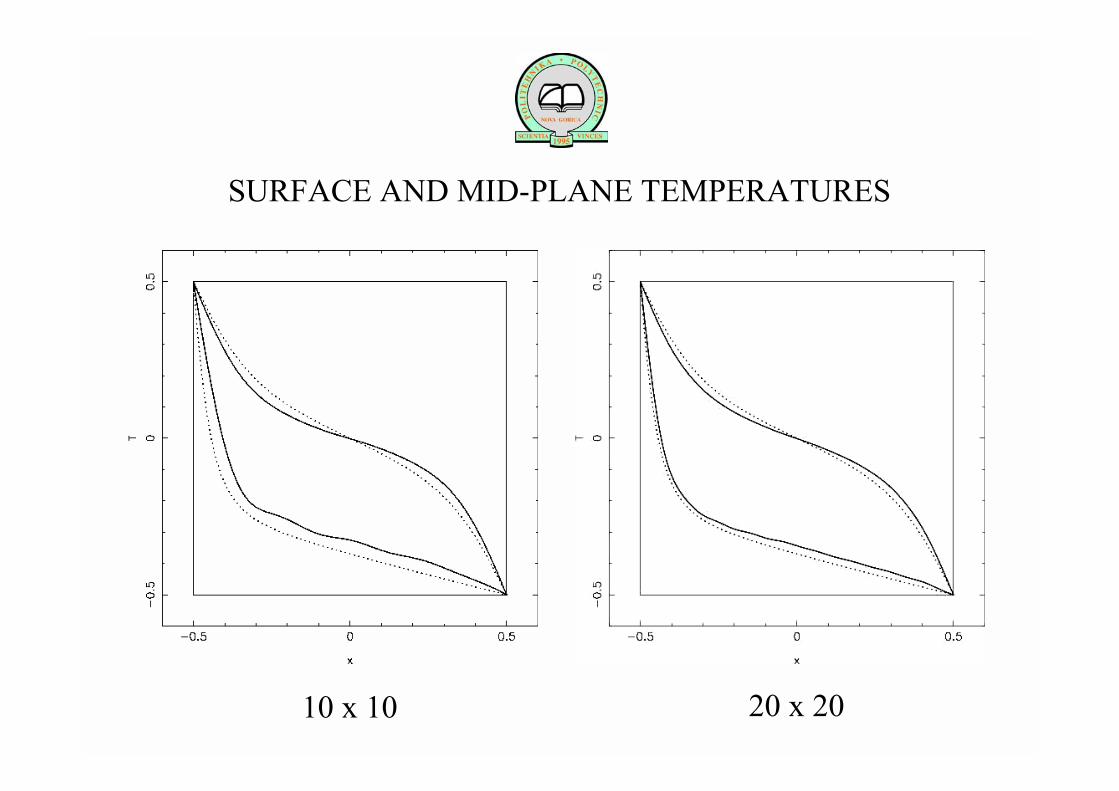
SURFACE AND MID-PLANE TEMPERATURES
10 x 10 20 x 20

SURFACE AND MID-PLANE TEMPERATURES
30 x 30 30 x 30 nonuniform
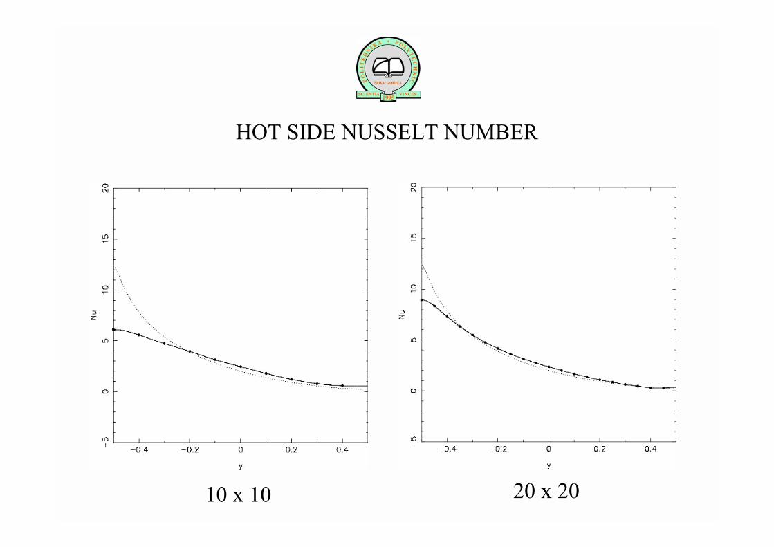
HOT SIDE NUSSELT NUMBER
10 x 10 20 x 20
HOT SIDE NUSSELT NUMBER
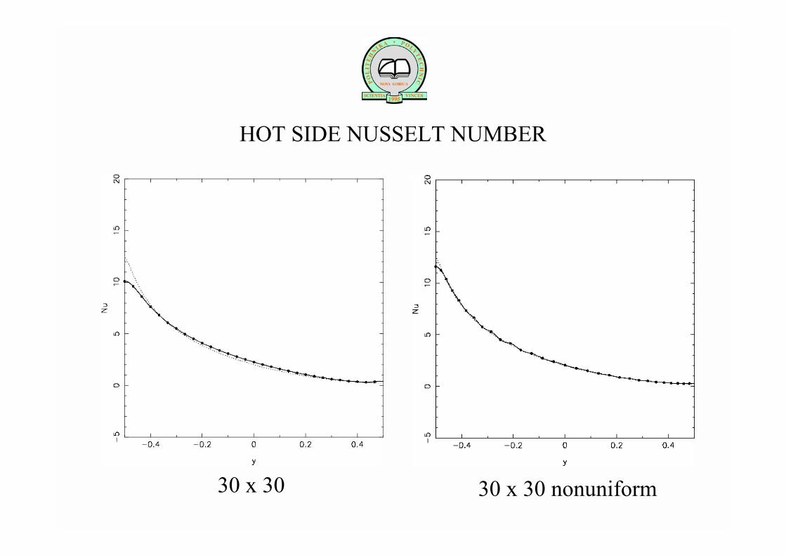
30 x 30 30 x 30 nonuniform
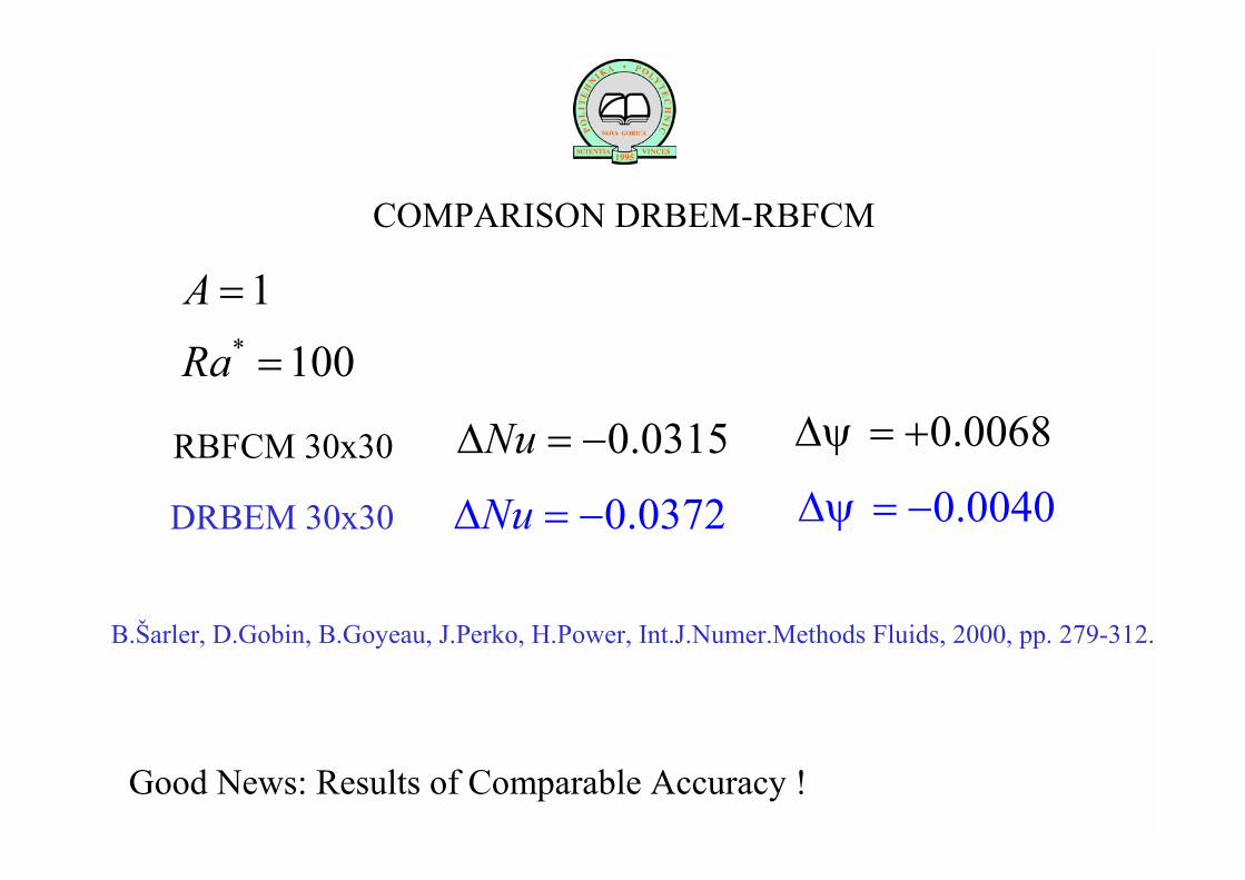
0.0372Nu∆ = − 0.0040ψ∆ = −DRBEM 30x30
0.0315Nu∆ = − 0.0068ψ∆ = +
COMPARISON DRBEM-RBFCM
B.arler, D.Gobin, B.Goyeau, J.Perko, H.Power, Int.J.Numer.Methods Fluids, 2000, pp. 279-312.
RBFCM 30x30
*
1100
ARa=
=
Good News: Results of Comparable Accuracy !

HIGHER ORDER THIN PLATE SPLINES
Results Diverge !
*
1100
ARa=
=
6
8
10
logloglog
r rr rr r
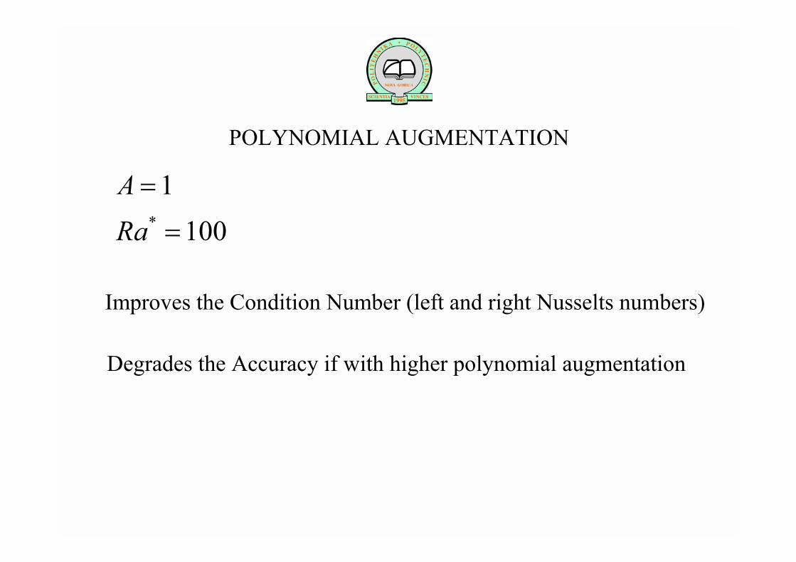
POLYNOMIAL AUGMENTATION
Improves the Condition Number (left and right Nusselts numbers)
*
1100
ARa=
=
Degrades the Accuracy if with higher polynomial augmentation
A=1
Ra=100
Da=10e-3
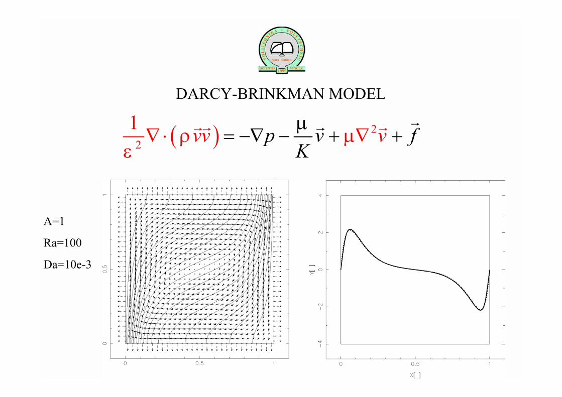
( ) 22
1 p v fK
v vvρ µε
µ= −∇ − + +∇ ⋅ ∇
rr r rr
DARCY-BRINKMAN MODEL

MESHFREE RBF COLLOCATION METHODJ.Perko, B.arler, C.S.Chen (2001)
natural convection in a single phase system natural convection in a solid-liquid system


MODULAR BRICK TB39

TB39

TB39 T10

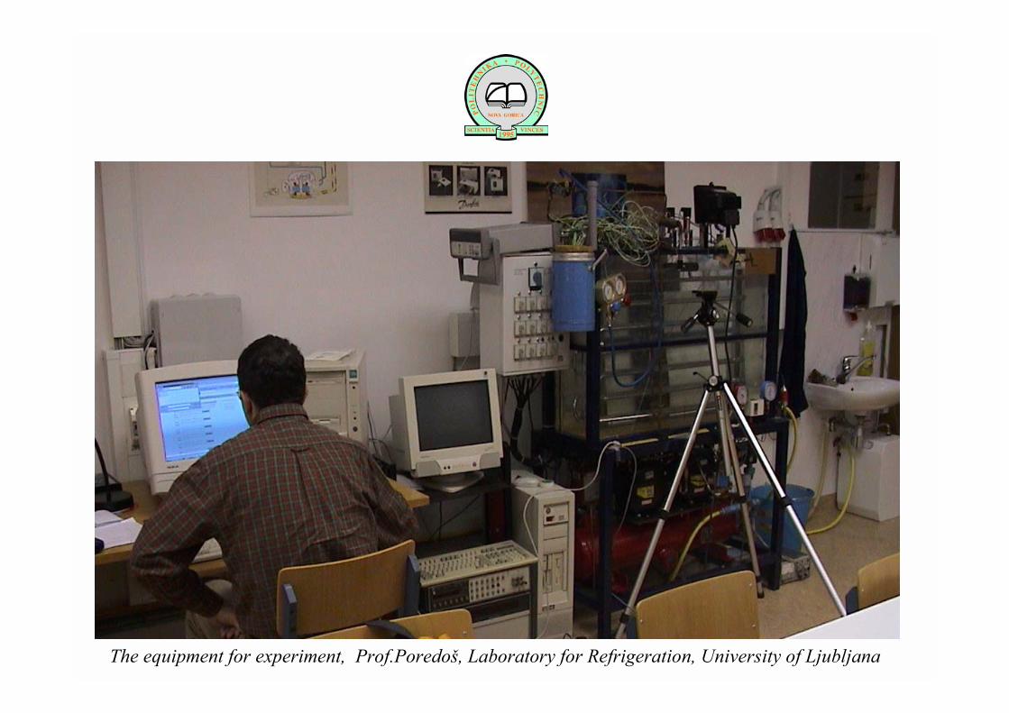
The equipment for experiment, Prof.Poredo, Laboratory for Refrigeration, University of Ljubljana
86
620
188
59
72
230
43
115
Ø16
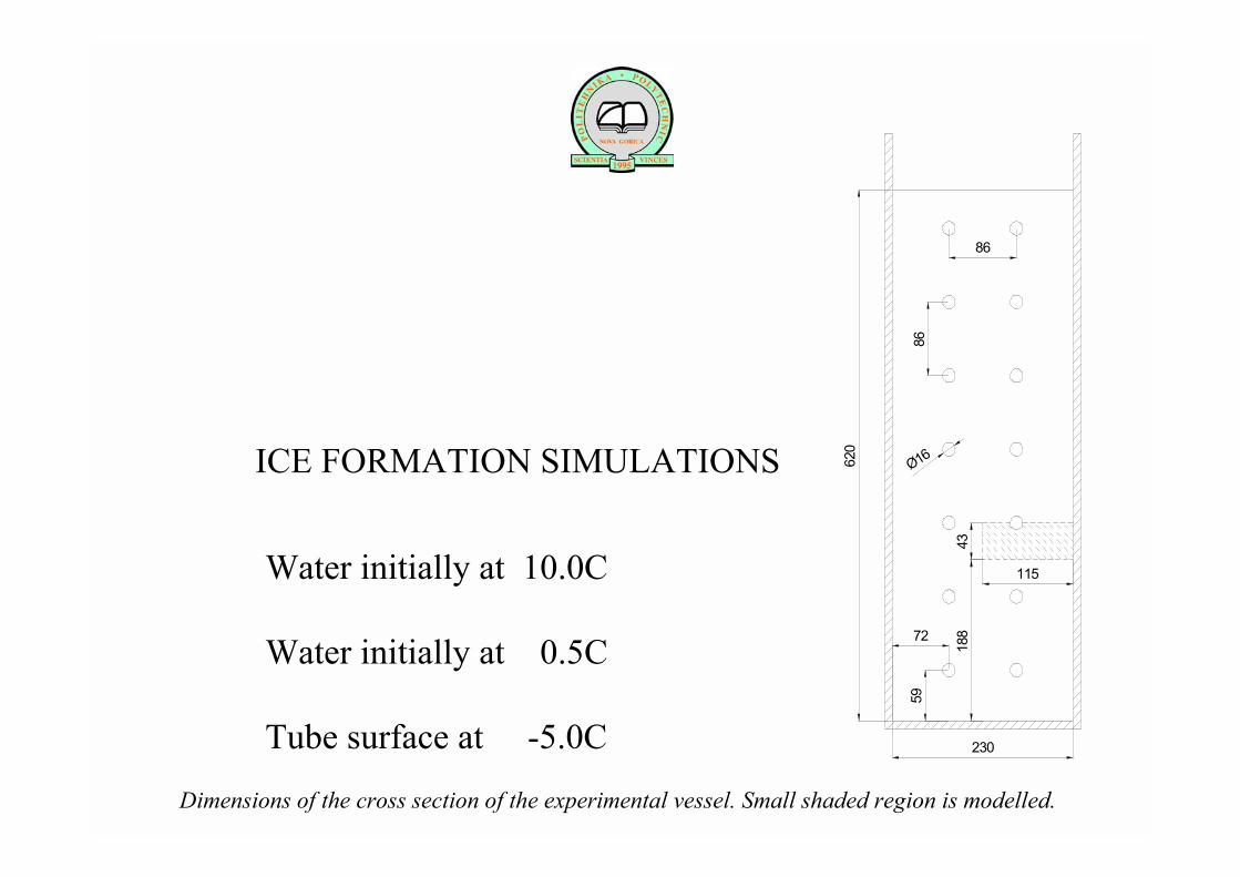
86
Dimensions of the cross section of the experimental vessel. Small shaded region is modelled.
ICE FORMATION SIMULATIONS
Water initially at 10.0C
Water initially at 0.5C
Tube surface at -5.0C
ICE FORMATION SIMULATIONS
One-domain temperature formulation
Voller-Swaminathan scheme
Most simple RBFCM using multiquadrics

B
A4.3
Grid Type I. Grid Type I includes 307 gridpoints, 76 on the boundaries and 231 in the domain.
A
B
2.15
Grid Type II. Grid Type II includes 1199 gridpoints, 150 on the boundaries and 1049 in the domain.
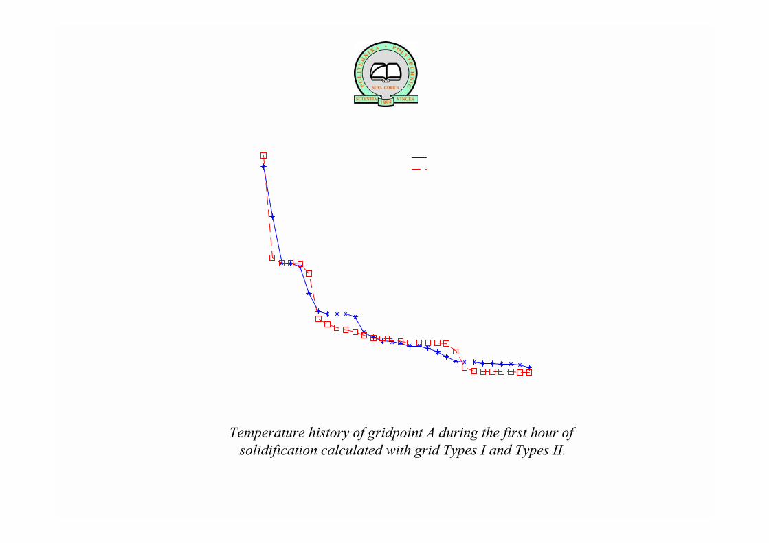
Temperature history of gridpoint A during the first hour of solidification calculated with grid Types I and Types II.

Temperature history of gridpoint B during the first two hours ofsolidification calculated with grid Type I and Type II.
0 0.01 0.02 0.03 0.04 0.05 0.06 0.07 0.08 0.09 0.1 0.11
0.18
0.19
0.2
0.21
0.22
0.23
0.24
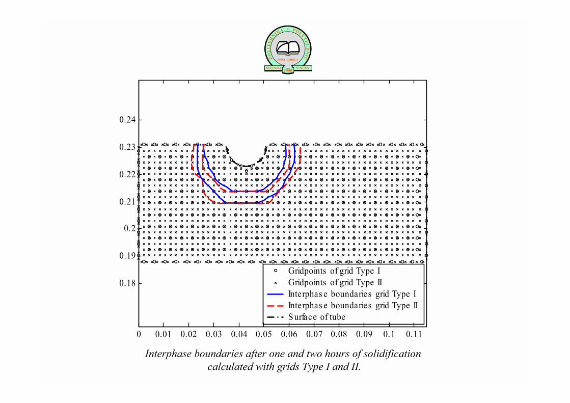
Gridpoints of grid Type IGridpoints of grid Type IIInterphas e boundaries grid Type IInterphas e boundaries grid Type IIS urface of tube
Interphase boundaries after one and two hours of solidification calculated with grids Type I and II.

0 300 600 900 1200 1500 1800 2100 2400 2700 3-6
-4
-2
0
2
4
6
8
Time (s )
Tem
pera
ture
(C)
Gridpoint A
Temperature histories of gridpoint A calculated with three time-steps

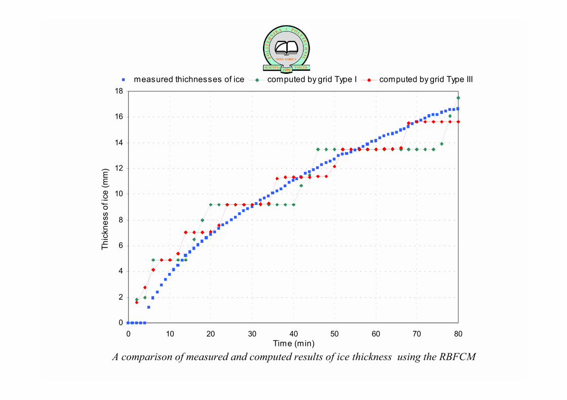
Grid Type III for numerical computation of ice thickness. Grid Type III includes 580 gridpoints,92 on the boundaries and 488 in the domain.
0
2
4
6
8
10
12
14
16
18
0 10 20 30 40 50 60 70 80Time (min)
Thic
knes
s of
ice
(mm
)
measured thichnesses of ice computed by grid Type I computed by grid Type III
A comparison of measured and computed results of ice thickness using the RBFCM

Promissing development and use of RBFCM for different transport phenomena
Method is very simple for numerical implementation
No need for polygonisation of the domain and boundary
2D and 3D numerical implementation is almost identical
Full matrices
Matrices might be ill conditioned
CONCLUSIONS

Fasshauers symmetric formulation
double consideration of boundary points in recirculating flow situations
compactly supported RBF
multilevel RBF
automatic domain decomposition
p - adaptivity through free parameters in RBF
r - adaptivity (elliptic mesh generator)
PRESENT RESEARCH


HOMOGENOUS SOLUTION BOUNDARY ELEMENT METHODS
Phase Change with Convection - Modelling and Validation, Udine, Italy, September 2-6, 2002.
0 ** 0 * 0( ) ( , ) ( ) ( , ) ( ) ( ) 0cp p s d p p s s s
n nψ
ψ ψΓ ΓΓ Γ
∂Φ ∂Γ − Φ − Φ =
∂ ∂∫ ∫rr r r r r r r r
* 01( , ) log( )2 | |
rp sp s
ψπ
=−
r rr r
* 1 1( , )4 | |
p sp s
ψπ
=−
r rr r
2D
3D
Drawback: boundary polygonisation, complicated integrals

HOMOGENOUS SOLUTIONMETHOD OF FUNDAMENTAL SOLUTIONS
Phase Change with Convection - Modelling and Validation, Udine, Italy, September 2-6, 2002.
0 *( , )n np sψ ζ ∗Φ =r r
1 3 1colN Nψ ψ
Γ Γ
∗ ∗+ −= =
02 2colN N x xp pψ ψ
Γ Γ
∗ ∗+ −= = −
03 1colN N y yp pψ ψ
Γ Γ
∗ ∗+ −= = −
04colN N z zp pψ ψ
Γ Γ
∗ ∗+ = = −
2 *( , ) 0n np sψ ζ ∗∇ =r r
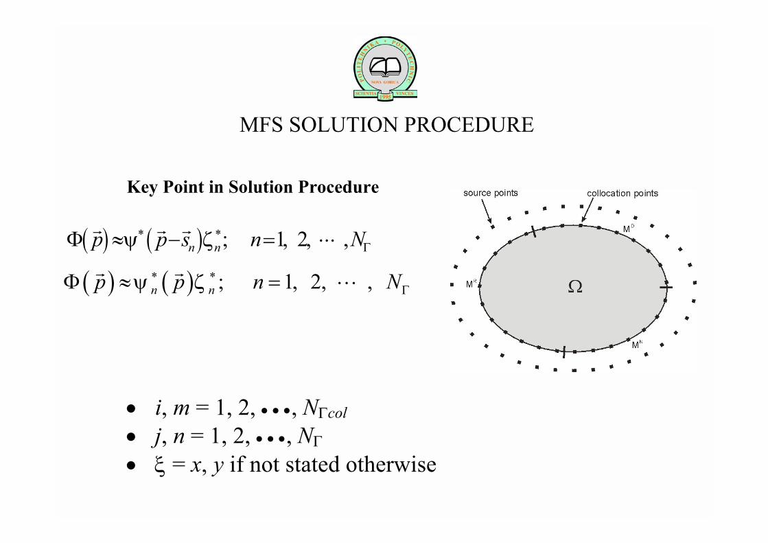
MFS SOLUTION PROCEDURE
• i, m = 1, 2, • • •, NΓcol
• j, n = 1, 2, • • •, NΓ
• ξ = x, y if not stated otherwise
( ) ( ) ; 1, 2, ,n np p s n Nψ ζ∗ ∗ΓΦ ≈ − = ⋅⋅⋅
r r r
Key Point in Solution Procedure
( ) ( ) ; 1, 2, ,n np p n Nψ ζ∗ ∗ΓΦ ≈ = ⋅⋅⋅
r r
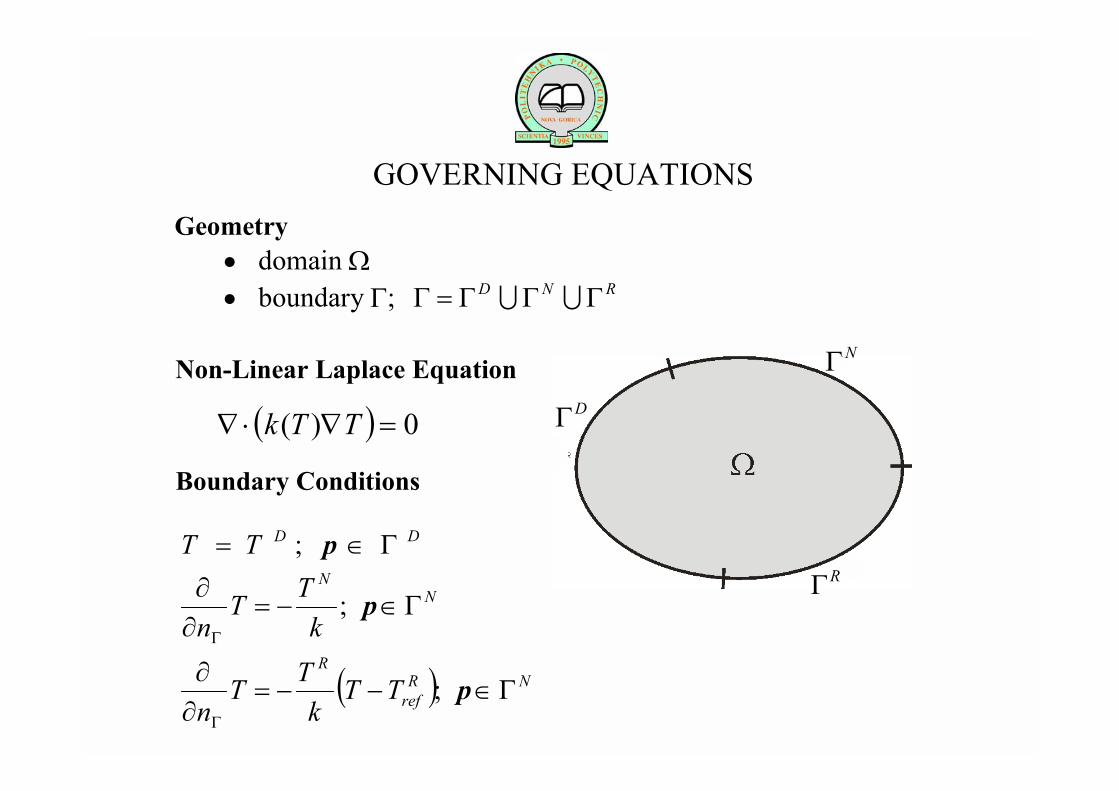
GOVERNING EQUATIONSGeometry
Non-Linear Laplace Equation
Boundary Conditions
• domain Ω• boundary Γ; RND ΓΓΓ=Γ UU
( ) 0)( =∇⋅∇ TTk
DDTT Γ∈= p;
NN
kTT
nΓ∈−=
∂∂
Γ
p;
( ) NRref
R
TTk
TTn
Γ∈−−=∂∂
Γ
p;
DΓ
NΓ
RΓ
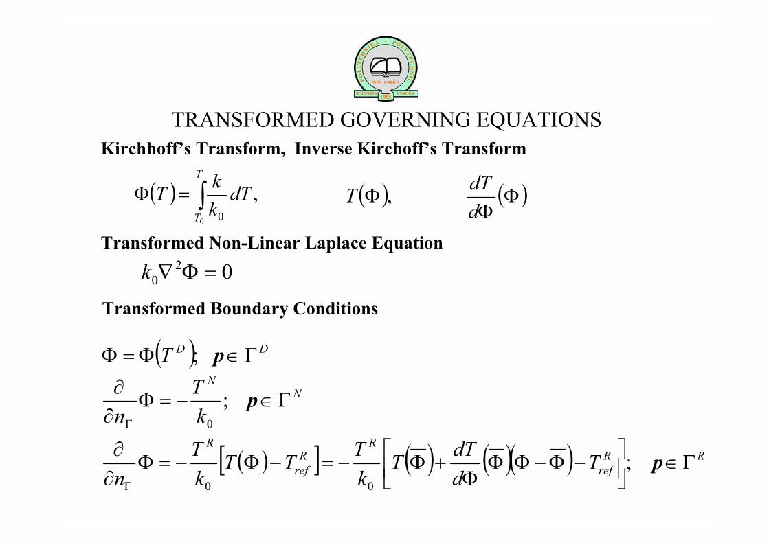
TRANSFORMED GOVERNING EQUATIONSKirchhoffs Transform, Inverse Kirchoffs Transform
Transformed Non-Linear Laplace Equation
Transformed Boundary Conditions
( ) DDT Γ∈Φ=Φ p;
NN
kT
nΓ∈−=Φ
∂∂
Γ
p;0
( )[ ] ( ) ( )( ) RRref
RR
ref
R
TddTT
kTTT
kT
nΓ∈
−Φ−ΦΦ
Φ+Φ−=−Φ−=Φ
∂∂
Γ
p;00
( ) ∫=ΦT
T
dTkkT
0
,0
( ) ( )ΦΦ
ΦddTT ,
020 =Φ∇k
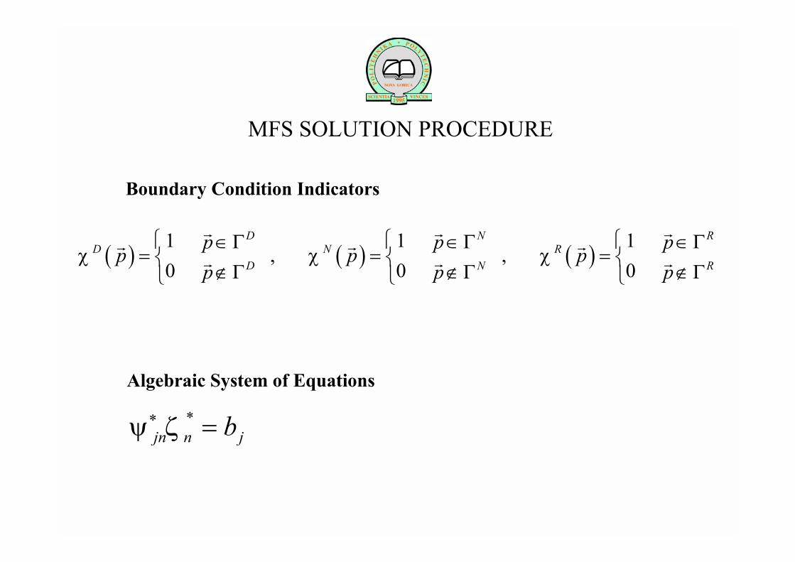
MFS SOLUTION PROCEDURE
Boundary Condition Indicators
( ) ( ) ( )1 1 1, ,
0 0 0
D N RD N R
D N R
p p pp p p
p p pχ χ χ
∈Γ ∈Γ ∈Γ= = =
∉Γ ∉Γ ∉Γ
r r rr r r
r r r
jnjn b=∗ *ζψ
Algebraic System of Equations

MFS SOLUTION PROCEDURE
first NΓ equations
( )ΦΦ∂
∂+
∂∂
+= ∗
Γ
∗
Γ
∗∗
ddT
kT
nn
R
inRiin
Niin
Diin
0
ψχψχψχψ
( ) ( ) ( )
−ΦΦ
Φ−Φ
−+
−+Φ= R
ref
RRi
NNi
DDii T
ddTT
kT
kTTb
00
χχχ
( )in nψ ψ p∗ ∗=r
remaining NΓ - NΓcol augmentation equations
( ) 1 2; , , ,jn nj j col colψ ψ p j N N N∗ ∗ ∗Γ + Γ + Γ= = = ⋅⋅⋅
rψ
,,,;0 21 Γ+Γ+Γ== NNNjb colcolj
( ) 1 20; , , , .n col colψ p j N N N∗Γ + Γ + Γ= = ⋅⋅⋅
r
MFS SOLUTION PROCEDURE
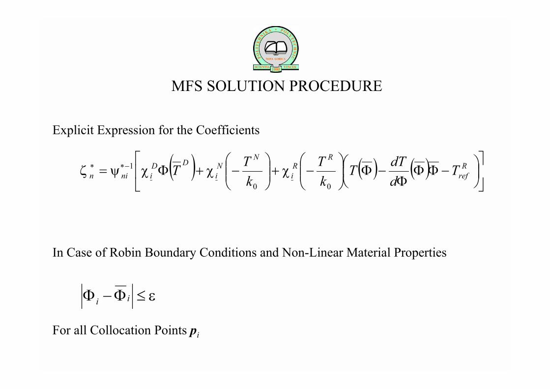
( ) ( ) ( )
−ΦΦ
Φ−Φ
−+
−+Φ= −∗∗ R
ref
RRi
NNi
DDinin T
ddTT
kT
kTT
00
1 χχχζ ψ
In Case of Robin Boundary Conditions and Non-Linear Material Properties
ε≤Φ−Φ ii
For all Collocation Points pi
Explicit Expression for the Coefficients
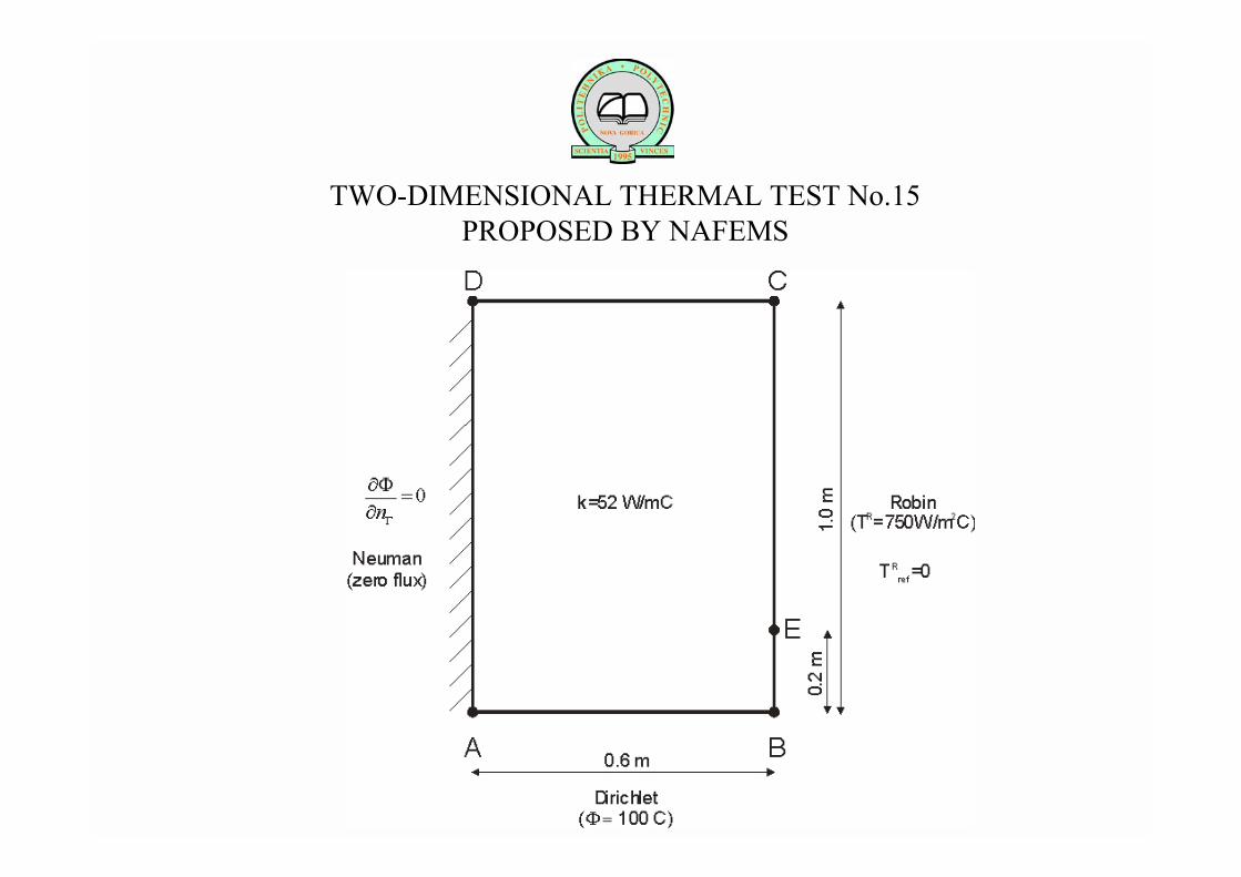
TWO-DIMENSIONAL THERMAL TEST No.15PROPOSED BY NAFEMS
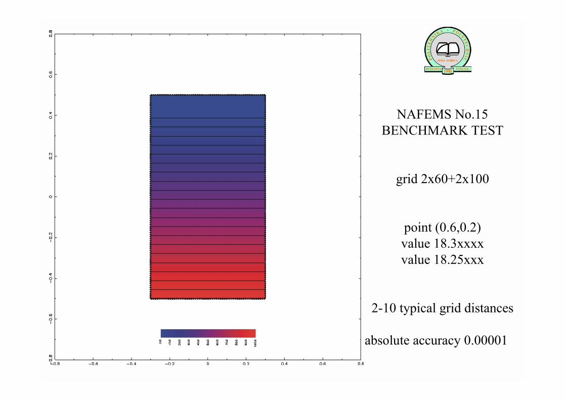
NAFEMS No.15 BENCHMARK TEST
grid 2x60+2x100
point (0.6,0.2)value 18.3xxxx value 18.25xxx
2-10 typical grid distances
absolute accuracy 0.00001
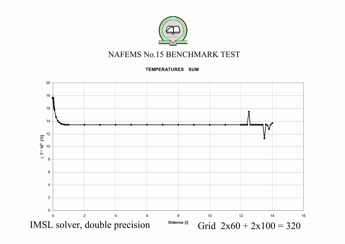
NAFEMS No.15 BENCHMARK TEST
TEMPERATURES SUM
0
2
4
6
8
10
12
14
16
18
20
0 2 4 6 8 10 12 14 16
Distance [/]
Σ T
* 10
5 [°C
]
Grid 2x60 + 2x100 = 320IMSL solver, double precision

14,0
15,0
16,0
17,0
18,0
19,0
20,0
21,0
22,0
23,0
24,0
Grid size
T [C
]
0.5 grid distance 1 grid distance 5 grid distance 6 grid distance
2x2 3x5 6x10 9x15 12x20 15x25 30x50 45x75 60x100 90x150 120x200 180x300 240x400
NAFEMS No.15 BENCHMARK TEST
SOLUTON AT DIFFERENT GRID DENSITY AND SOURCE DISTANCE

0,000
0,001
0,010
0,100
1,000
10,000
Grid size
log ∆
T [C
]
0.5 grid distance 1 grid distance 5 grid distance 6 grid distance
2x2 3x5 6x10 9x15 12x20 15x25 30x50 45x75 60x100 90x150 120x200 180x300 240x400
NAFEMS No.15 BENCHMARK TEST- ABSOLUTE ERROR
ACCURACY AT DIFFERENT GRID DENSITY AND SOURCE DISTANCE

NUMERICAL EXAMPLES
WHERE IS THE PROPER POSITION OF SOURCE POINTS ?
WHERE POSITION CHANGE DOES NOT INFLUENCE THE RESULTS !

NUMERICAL EXAMPLES
CASE WITH CONSTANT THERMAL CONDUCTIVITY
0.6 WkmK
=
( )[ 0.6 0.005 ]
0.5 0.7
o
o
T C WkC m K
W Wkm K m K
= −
≤ ≤
CASE WITH TEMPERATURE DEPENDENT THERMAL CONDUCTIVITY
conservative 30%
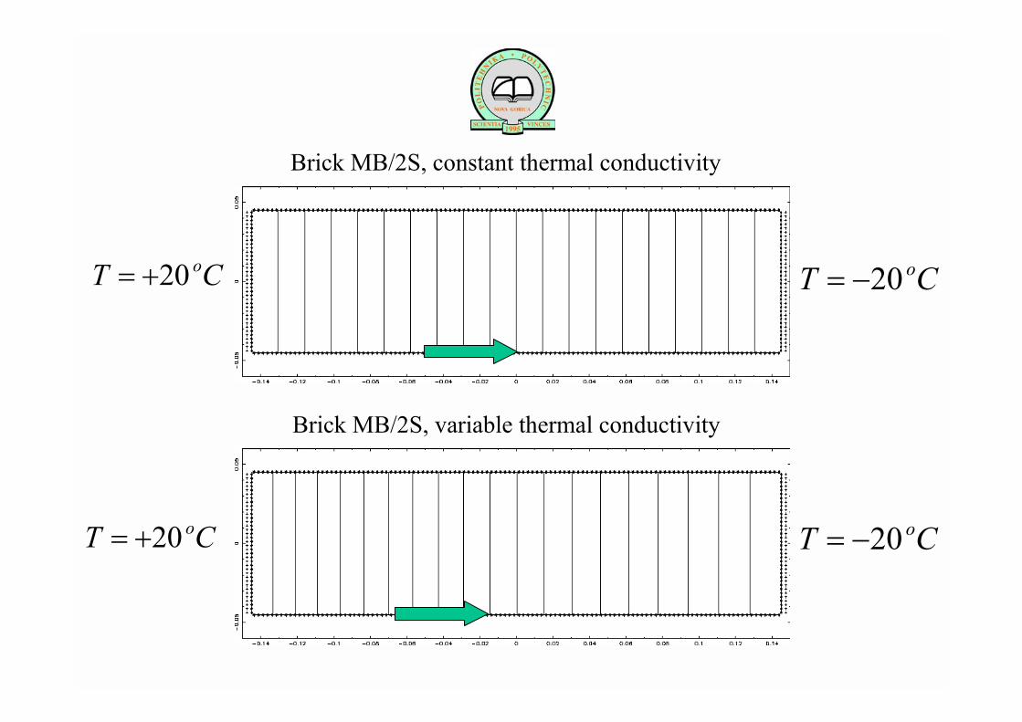
Brick MB/2S, constant thermal conductivity
Brick MB/2S, variable thermal conductivity
20 oT C= + 20 oT C= −
20 oT C= + 20 oT C= −
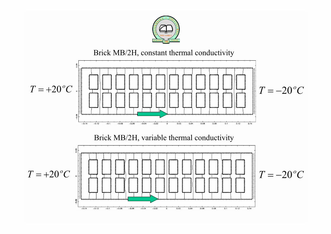
Brick MB/2H, constant thermal conductivity
Brick MB/2H, variable thermal conductivity
20 oT C= +
20 oT C= +
20 oT C= −
20 oT C= −

BRICK TB39 - NUMERICAL RESULTS
number of collocation nodes = 4552, computing time = 5min (PIII, 933 MHz), COMPAQ FORTRAN+IMSL

BRICK TB39 - ALTERNATIVE, NUMERICAL RESULTS
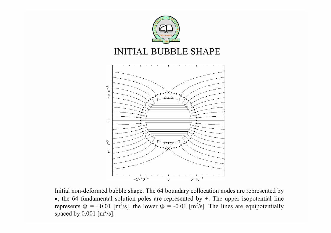
INITIAL BUBBLE SHAPE
Initial non-deformed bubble shape. The 64 boundary collocation nodes are represented by•, the 64 fundamental solution poles are represented by +. The upper isopotential linerepresents Φ = +0.01 [m2/s], the lower Φ = -0.01 [m2/s]. The lines are equipotentiallyspaced by 0.001 [m2/s].
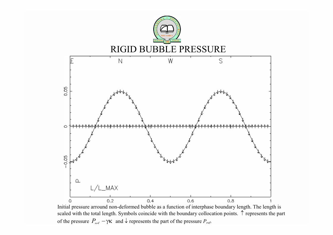
RIGID BUBBLE PRESSURE
Initial pressure arround non-deformed bubble as a function of interphase boundary length. The length isscaled with the total length. Symbols coincide with the boundary collocation points. ↑ represents the partof the pressure γκ−refP and ↓ represents the part of the pressure Pref.
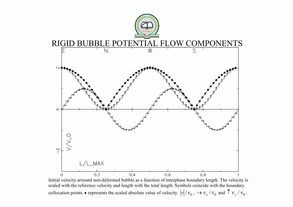
RIGID BUBBLE POTENTIAL FLOW COMPONENTS
Initial velocity arround non-deformed bubble as a function of interphase boundary length. The velocity isscaled with the reference velocity and length with the total length. Symbols coincide with the boundarycollocation points. • represents the scaled absolute value of velocity 0/ vv , 0/ vvx→ and ./ 0vvy↑
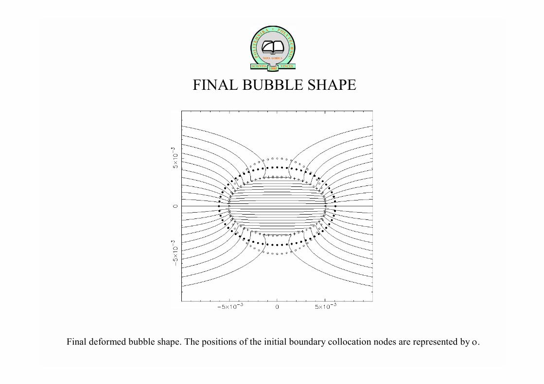
FINAL BUBBLE SHAPE
Final deformed bubble shape. The positions of the initial boundary collocation nodes are represented by ο.

FINAL BUBBLE PRESSURE
(Almost) final pressure arround deformed bubble as a function of interphase boundary length.

FINAL POTENTIAL FLOW COMPONENTS
Final velocity arround deformed bubble as a function of interphase boundary length.
SOLUTION PROCEDURE
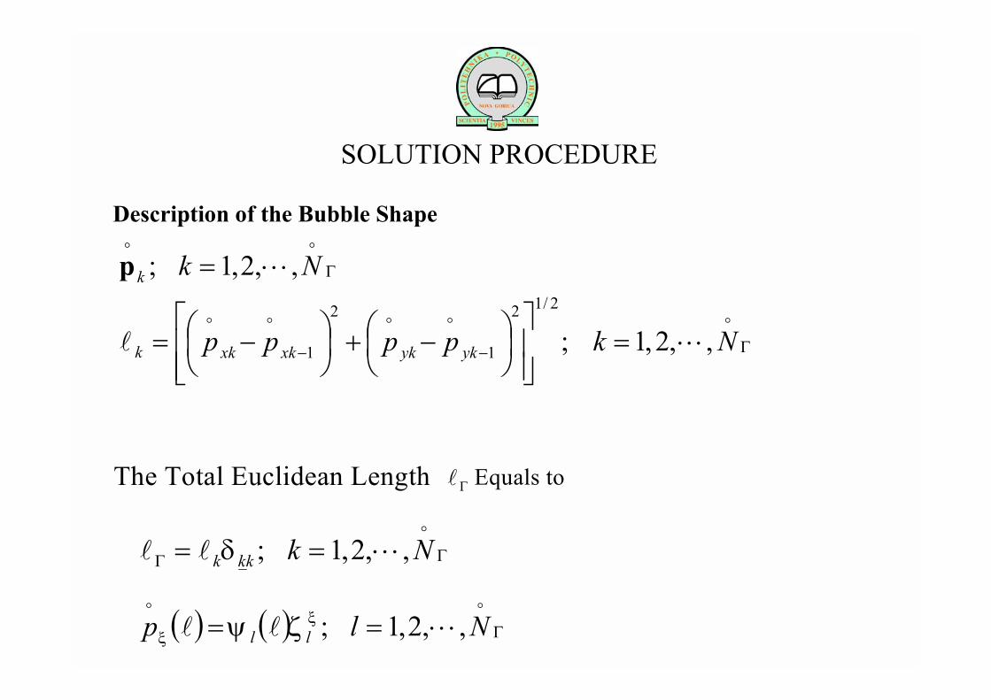
Description of the Bubble Shape
Γ⋅⋅⋅=oo
Nkk ,,2,1;p
Γ−− ⋅⋅⋅=
−+
−=
ooooo
l Nkpppp ykykxkxkk ,,2,1;2/12
1
2
1
The Total Euclidean Length Γl Equals to
ΓΓ ⋅⋅⋅==o
ll Nkkkk ,,2,1;δ
( ) ( ) Γ⋅⋅⋅==oo
ll Nlp ll ,,2,1;ξξ ζψ

SOLUTION PROCEDURE
Cubic Splines
( ) ΓΝ⋅⋅⋅=−=o
lll ,,2,1;3 kkkψ
( ) ( ) 121
==−Γ+Γ Νll oo ψψ
N
( ) ( ) lll oo ==−Γ+Γ Ν 12
ψψN
( ) ( ) 3
3
lll oo ==Γ+Γ Ν
ψψN
3 Augmented Functions

SOLUTION PROCEDURECompatibility Conditions
( ) ( ) ,0 ξξ ζψζψ llll =Γl ( ) ( ) ,0 ξξ ζψζψ llll dd
dd
ll
l=Γ ( ) ( ) ξξ ζψζψ llll d
ddd 02
2
2
2Γ
ΓΓ =
ll
l
ΓΝ⋅⋅⋅==o
,,2,1,; ljb jljlξξ ζψ
( ) ΓΓ Ν⋅⋅⋅=⋅⋅⋅==oo
l ,,2,1,,,2,1; lNkklkl ψξψ
Γ⋅⋅⋅==oo
Nlpb ll ,,2,1;ξξ
jljl pξξξζ
o1−= ψ
( ) ( ),02 ll ψψξ −= ΓΝ −Γ
lψ 02=
−ΓΝb
( ) ( ),01 ll ψψξ
ll
l ∂∂
−∂∂
= ΓΝ −Γψ 0
1=
−ΓΝb
( ) ( ),02
2
2
2
ll ψψξ
ll
l ∂∂
−∂∂
= ΓΝΓψ 0
1=
−ΓΝb
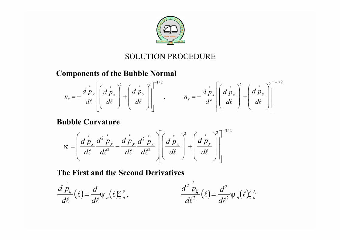
SOLUTION PROCEDURE
Components of the Bubble Normal
,
2/122−
+
+=
lll
ooo
dpd
dpd
dpd
n yxyx
2/122−
+
−=
lll
ooo
dpd
dpd
dpdn yxx
y
Bubble Curvature2/322
2
2
2
2
−
+
−=
llllll
oooooo
dpd
dpd
dpd
dpd
dpd
dpd yxxyyxκ
The First and the Second Derivatives
( ) ( ) ,ξξ ζψ nndd
dpd
ll
ll
o
= ( ) ( ) ξξ ζψ nndd
dpd
ll
ll
o
2
2
2
2
=


![í]b|:^ ì[v ó ²'¨ M Z#. Z8{ Ç ä d 9×'¼ S6Û Û · 2019-07-15 · Áå»»ÜÝ pppppppppppppppppp pp 2 4 Áå¹ Ëݺ§å² ppppppppppppp 2 5 ¹ «¡¢Û å²î ppppppppppppp](https://img.dokumen.tips/doc/110x75/5f7479ea643b4c5c17509853/b-v-m-z-z8-d-9-s6-2019-07-15-oe.jpg)


![¨¶§³°¬´¹¯ GF ]o &9 pppppp ppppppppppppp · [ V ] W R k m lÐ x¹ NK 6 Ë û Æ ò ç Ø õ ã Ë û Æ ò ç Ø õ ã ´ oY Eë 9< ! d ÿà ; jx îO j £ ì t Ú Ä èO](https://img.dokumen.tips/doc/110x75/607dfc0b7ab9cb48d05b1c5b/-gf-o-9-pppppp-v-w-r-k-m-l-x-nk-6-.jpg)


![Konwekcja magnetyczna cieczy paramagnetycznej w naczyniu …fluid.ippt.gov.pl/seminar/text/fornalik17022010.pdf · Podatność magnetyczna χg [m 3/kg] jest to wielkość fizyczna](https://img.dokumen.tips/doc/110x75/5c79852f09d3f294278ca1d5/konwekcja-magnetyczna-cieczy-paramagnetycznej-w-naczyniu-fluidipptgovplseminartext.jpg)